Brian S. Everitt A Handbook of Statistical Analyses using SPSS

A Handbook of 

Statistical Analyses 

using SPSS 

Sabine Landau 

and 

Brian S. Everitt 

CHAPMAN & HALL/CRC 

A CRC Press Company 

Boca Raton London New York Washington, D.C. 

© 2004 by Chapman & Hall/CRC Press LLC

Library of Congress Cataloging-in-Publication Data 

Landau, Sabine. 

A handbook of statistical analyses using SPSS / Sabine, Landau, Brian S. Everitt. 

p. cm. 

Includes bibliographical references and index. 

ISBN 1-58488-369-3 (alk. paper) 

1. SPSS ( Computer file). 2. Social sciences—Statistical methods—Computer programs. 3. 

Social sciences—Statistical methods—Data processing. I. Everitt, Brian S. II. Title. 

HA32.E93 2003 

519.50285—dc22 2003058474 

This book contains information obtained from authentic and highly regarded sources. Reprinted material 

is quoted with permission, and sources are indicated. A wide variety of references are listed. Reasonable 

efforts have been made to publish reliable data and information, but the author and the publisher cannot 

assume responsibility for the validity of all materials or for the consequences of their use. 

Neither this book nor any part may be reproduced or transmitted in any form or by any means, electronic 

or mechanical, including photocopying, microfilming, and recording, or by any information storage or 

retrieval system, without prior permission in writing from the publisher. 

The consent of CRC Press LLC does not extend to copying for general distribution, for promotion, for 

creating new works, or for resale. Specific permission must be obtained in writing from CRC Press LLC 

for such copying. 

Direct all inquiries to CRC Press LLC, 2000 N.W. Corporate Blvd., Boca Raton, Florida 33431. 

Trademark Notice: Product or corporate names may be trademarks or registered trademarks, and are 

used only for identification and explanation, without intent to infringe. 

Visit the CRC Press Web site at www.crcpress.com 

© 2004 by Chapman & Hall/CRC Press LLC 

No claim to original U.S. Government works 

International Standard Book Number 1-58488-369-3 

Library of Congress Card Number 2003058474 

Printed in the United States of America 1 2 3 4 5 6 7 8 9 0 

Printed on acid-free paper 


Preface 

SPSS, standing for Statistical Package for the Social Sciences, is a powerful, 

user-friendly software package for the manipulation and statistical analysis 

of data. The package is particularly useful for students and researchers in 

psychology, sociology, psychiatry, and other behavioral sciences, containing 

as it does an extensive range of both univariate and multivariate 

procedures much used in these disciplines. Our aim in this handbook is 

to give brief and straightforward descriptions of how to conduct a range 

of statistical analyses using the latest version of SPSS, SPSS 11. Each chapter 

deals with a different type of analytical procedure applied to one or more 

data sets primarily (although not exclusively) from the social and behavioral 

areas. Although we concentrate largely on how to use SPSS to get 

results and on how to correctly interpret these results, the basic theoretical 

background of many of the techniques used is also described in separate 

boxes. When more advanced procedures are used, readers are referred 

to other sources for details. Many of the boxes contain a few mathematical 

formulae, but by separating this material from the body of the text, we 

hope that even readers who have limited mathematical background will 

still be able to undertake appropriate analyses of their data. 

The text is not intended in any way to be an introduction to statistics 

and, indeed, we assume that most readers will have attended at least one 

statistics course and will be relatively familiar with concepts such as linear 

regression, correlation, significance tests, and simple analysis of variance. 

Our hope is that researchers and students with such a background will 

find this book a relatively self-contained means of using SPSS to analyze 

their data correctly. 

Each chapter ends with a number of exercises, some relating to the 

data sets introduced in the chapter and others introducing further data 

sets. Working through these exercises will develop both SPSS and statistical 

skills. Answers to most of the exercises in the text are provided at 


http://www.iop.kcl.ac.uk/iop/departments/BioComp/SPSSBook.shtml. 

The majority of data sets used in the book can be found at the same site. 

We are grateful to Ms. Harriet Meteyard for her usual excellent word 

processing and overall support during the writing of this book. 


Sabine Landau and Brian Everitt 

London, July 2003

Distributors 

The distributor for SPSS in the United Kingdom is 

SPSS U.K. Ltd. 

1st Floor St. Andrew’s House, West Street 

Woking 

Surrey, United Kingdom GU21 6EB 

Tel. 0845 3450935 

FAX 01483 719290 

Email sales@spss.co.uk 

In the United States, the distributor is 

SPSS Inc. 

233 S. Wacker Drive, 11th floor 

Chicago, IL 60606-6307 

Tel. 1(800) 543-2185 

FAX 1(800) 841-0064 

Email sales@spss.com 


Contents 

Preface 

Distributors 

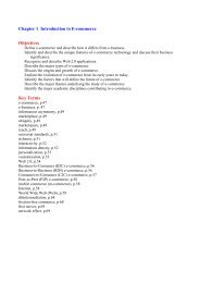
1 A Brief Introduction to SPSS 

1.1 Introduction 

1.2 Getting Help 

1.3 Data Entry 

1.3.1 The Data View Spreadsheet 

1.3.2 The Variable View Spreadsheet 

1.4 Storing and Retrieving Data Files 

1.5 The Statistics Menus 

1.5.1 Data File Handling 

1.5.2 Generating New Variables 

1.5.3 Running Statistical Procedures 

1.5.4 Constructing Graphical Displays 

1.6 The Output Viewer 

1.7 The Chart Editor 

1.8 Programming in SPSS 

2 Data Description and Simple Inference for Continuous 

Data: The Lifespans of Rats and Ages at Marriage in the 

U.S. 

2.1 Description of Data 

2.2 Methods of Analysis. 

2.3 Analysis Using SPSS 

2.3.1 Lifespans of Rats 

2.3.2 Husbands and Wives 

2.4 Exercises 

2.4.1 Guessing the Width of a Lecture Hall 

2.4.2 More on Lifespans of Rats: Significance Tests for Model 

Assumptions 

2.4.3 Motor Vehicle Theft in the U.S. 

2.4.4 Anorexia Nervosa Therapy 

2.4.5 More on Husbands and Wives: Exact Nonparametric Tests 


3 Simple Inference for Categorical Data: From Belief in 

the Afterlife to the Death Penalty and Race 


3.2 Methods of Analysis 


3.3.1 Husbands and Wives Revisited. 

3.3.2 Lifespans of Rats Revisited 

3.3.3 Belief in the Afterlife 

3.3.4 Incidence of Suicidal Feelings 

3.3.5 Oral Contraceptive Use and Blood Clots 

3.3.6 Alcohol and Infant Malformation 

3.3.7 Death Penalty Verdicts 

3.4 Exercises 

3.4.1 Depersonalization and Recovery from Depression 

3.4.2 Drug Treatment of Psychiatric Patients: Exact Tests for 

Two-Way Classifications 

3.4.3 Tics and Gender 

3.4.4 Hair Color and Eye Color 

4 Multiple Linear Regression: Temperatures in America 

and Cleaning Cars 


4.2 Multiple Linear Regression 


4.3.1 Cleaning Cars 

4.3.2 Temperatures in America 

4.4 Exercises. 

4.4.1 Air Pollution in the U.S. 

4.4.2 Body Fat 

4.4.3 More on Cleaning Cars: Influence Diagnostics 

5 Analysis of Variance I: One-Way Designs; Fecundity of 

Fruit Flies, Finger Tapping, and Female Social Skills. 


5.2 Analysis of Variance. 


5.3.1 Fecundity of Fruit Flies . 

5.3.2 Finger Tapping and Caffeine Consumption. 

5.3.3 Social Skills of Females 

5.4 Exercises. 

5.4.1 Cortisol Levels in Psychotics: Kruskal-Wallis Test 

5.4.2 Cycling and Knee-Joint Angles 

5.4.3 More on Female Social Skills: Informal Assessment of 

MANOVA Assumptions 


6 Analysis of Variance II: Factorial Designs; Does Marijuana 

Slow You Down? and Do Slimming Clinics Work? 


6.2 Analysis of Variance 


6.3.1 Effects of Marijuana Use 

6.3.2 Slimming Clinics 

6.4 Exercises 

6.4.1 Headache Treatments 

6.4.2 Biofeedback and Hypertension 

6.4.3 Cleaning Cars Revisited: Analysis of Covariance 

6.4.4 More on Slimming Clinics 

7 Analysis of Repeated Measures I: Analysis of Variance 

Type Models; Field Dependence and a Reverse Stroop 

Task 


7.2 Repeated Measures Analysis of Variance 


7.4 Exercises 

7.4.1 More on the Reverse Stroop Task 

7.4.2 Visual Acuity Data. 

7.4.3 Blood Glucose Levels 

8 Analysis of Repeated Measures II: Linear Mixed Effects 

Models; Computer Delivery of Cognitive Behavioral 

Therapy 


8.2 Linear Mixed Effects Models 


8.4 Exercises 

8.4.1 Salsolinol Levels and Alcohol Dependency 

8.4.2 Estrogen Treatment for Post-Natal Depression 

8.4.3 More on “Beating the Blues”: Checking the Model for 

the Correlation Structure 

9 Logistic Regression: Who Survived the Sinking of the 

Titanic? 


9.2 Logistic Regression 


9.4 Exercises 

9.4.1 More on the Titanic Survivor Data 

9.4.2 GHQ Scores and Psychiatric Diagnosis 

9.4.3 Death Penalty Verdicts Revisited 


10 Survival Analysis: Sexual Milestones in Women and 

Field Dependency of Children. 


10.2 Survival Analysis and Cox’s Regression 


10.3.1 Sexual Milestone Times 

10.3.2 WISC Task Completion Times 

10.4 Exercises 

10.4.1 Gastric Cancer 

10.4.2 Heroin Addicts 

10.4.3 More on Sexual Milestones of Females 

11 Principal Component Analysis and Factor Analysis: 

Crime in the U.S. and AIDS Patients’ Evaluations of 

Their Clinicians 


11.2 Principal Component and Factor Analysis 

11.2.1 Principal Component Analysis 

11.2.2 Factor Analysis 

11.2.3 Factor Analysis and Principal Components Compared 


11.3.1 Crime in the U.S. 

11.3.2 AIDS Patients’ Evaluations of Their Clinicians 



11.4.2 More on AIDS Patients’ Evaluations of Their Clinicians: 

Maximum Likelihood Factor Analysis 

12 Classification: Cluster Analysis and Discriminant 

Function Analysis; Tibetan Skulls 


12.2 Classification: Discrimination and Clustering 


12.3.1 Tibetan Skulls: Deriving a Classification Rule. 

12.3.2 Tibetan Skulls: Uncovering Groups. 


12.4.1 Sudden Infant Death Syndrome (SIDS) 

12.4.2 Nutrients in Food Data 

12.4.3 More on Tibetan Skulls 

References 


Chapter 1 

A Brief Introduction 

to SPSS 

1.1 Introduction 

The “Statistical Package for the Social Sciences” (SPSS) is a package of 

programs for manipulating, analyzing, and presenting data; the package 

is widely used in the social and behavioral sciences. There are several 

forms of SPSS. The core program is called SPSS Base and there are a 

number of add-on modules that extend the range of data entry, statistical, 

or reporting capabilities. In our experience, the most important of these 

for statistical analysis are the SPSS Advanced Models and SPSS Regression 

Models add-on modules. SPSS Inc. also distributes stand-alone programs 

that work with SPSS. 

There are versions of SPSS for Windows (98, 2000, ME, NT, XP), major 

UNIX platforms (Solaris, Linux, AIX), and Macintosh. In this book, we 

describe the most popular, SPSS for Windows, although most features are 

shared by the other versions. The analyses reported in this book are based 

on SPSS version 11.0.1 running under Windows 2000. By the time this 

book is published, there will almost certainly be later versions of SPSS 

available, but we are confident that the SPSS instructions given in each 

of the chapters will remain appropriate for the analyses described. 

While writing this book we have used the SPSS Base, Advanced Models, 

Regression Models, and the SPSS Exact Tests add-on modules. Other available 

add-on modules (SPSS Tables, SPSS Categories, SPSS Trends, SPSS 

Missing Value Analysis) were not used. 


1. SPSS Base (Manual: SPSS Base 11.0 for Windows User’s Guide): This 

provides methods for data description, simple inference for continuous 

and categorical data and linear regression and is, therefore, 

sufficient to carry out the analyses in Chapters 2, 3, and 4. It also 

provides techniques for the analysis of multivariate data, specifically 

for factor analysis, cluster analysis, and discriminant analysis (see 

Chapters 11 and 12). 

2. Advanced Models module (Manual: SPSS 11.0 Advanced Models): 

This includes methods for fitting general linear models and linear 

mixed models and for assessing survival data, and is needed to 

carry out the analyses in Chapters 5 through 8 and in Chapter 10. 

3. Regression Models module (Manual: SPSS 11.0 Regression Models): 

This is applicable when fitting nonlinear regression models. We have 

used it to carry out a logistic regression analysis (see Chapter 9). 

(The Exact Tests module has also been employed on occasion, specifically 

in the Exercises for Chapters 2 and 3, to generate exact p-values.) 

The SPSS 11.0 Syntax Reference Guide (SPSS, Inc., 2001c) is a reference 

for the command syntax for the SPSS Base system and the Regression 

Models and Advanced Models options. 

The SPSS Web site (http://www.spss.com/) provides information on 

add-on modules and stand-alone packages working with SPSS, events and 

SPSS user groups. It also supplies technical reports and maintains a 

frequently asked questions (FAQs) list. 

SPSS for Windows offers a spreadsheet facility for entering and browsing 

the working data file — the Data Editor. Output from statistical procedures 

is displayed in a separate window — the Output Viewer. It takes the 

form of tables and graphics that can be manipulated interactively and can 

be copied directly into other applications. 

It is its graphical user interface (GUI) that makes SPSS so easy by 

simply selecting procedures from the many menus available. It is the GUI 

that is used in this book to carry out all the statistical analysis presented. 

We also show how to produce command syntax for record keeping. 

We assume that the reader is already familiar with the Windows GUI 

and we do not spend much time discussing the data manipulation and 

result presentation facilities of SPSS for Windows. These features are 

described in detail in the Base User’s Guide (SPSS, Inc., 2001d). Rather 

we focus on the statistical features of SPSS — showing how it can be 

used to carry out statistical analyses of a variety of data sets and on how 

to interpret the resulting output. To aid in reading this text, we have 

adopted the Helvetica Narrow font to indicate spreadsheet column names, 

menu commands, and text in dialogue boxes as seen on the SPSS GUI. 


1.2 Getting Help 

Online help is provided from the Help menu or via context menus or Help 

buttons on dialogue boxes. We will mention the latter features when 

discussing the dialogue boxes and output tables. Here, we concentrate 

on the general help facility. The required menu is available from any 

window and provides three major help facilities: 

Help — Statistics Coach helps users unfamiliar with SPSS or the statistical 

procedures available in SPSS to get started. This facility prompts 

the user with simple questions in nontechnical language about 

the purpose of the statistical analysis and provides visual examples 

of basic statistical and charting features in SPSS. The facility covers 

only a selected subset of procedures. 

Help — Tutorial provides access to an introductory SPSS tutorial, including 

a comprehensive overview of SPSS basics. It is designed to 

provide a step-by-step guide for carrying out a statistical analysis 

in SPSS. All files shown in the examples are installed with the 

tutorial so the user can repeat the analysis steps. 

Help — Topics opens the Help Topics: SPSS for Windows box, which provides 

access to Contents, Index, and Find tabs. Under the Contents 

tab, double-clicking items with a book symbol expands or collapses 

their contents (the Open and Close buttons do the same). 

The Index tab provides an alphabetical list of topics. Once a topic 

is selected (by double-clicking), or the first few letters of the word 

are typed in, the Display button provides a description. The Find 

tab allows for searching the help files for specific words and 

phrases. 

1.3 Data Entry 

When SPSS 11.0 for Windows is first opened, a default dialogue box 

appears that gives the user a number of options. The Tutorial can be 

accessed at this stage. Most likely users will want to enter data or open 

an existing data file; we demonstrate the former (Display 1.1). Further 

options will be discussed later in this chapter. This dialogue box can be 

prevented from opening in the future by checking this option at the 

bottom of the box. 

When Type in data is selected, the SPSS Data Editor appears as an empty 

spreadsheet. At the top of the screen is a menu bar and at the bottom a 

status bar. The status bar informs the user about facilities currently active; 

at the beginning of a session it simply reads, “SPSS Processor is ready.” 


Display 1.1 Initial SPSS for Windows dialogue box. 

The facilities provided by the menus will be explained later in this chapter. 

SPSS also provides a toolbar for quick and easy access to common tasks. 

A brief description of each tool can be obtained by placing the cursor 

over the tool symbol and the display of the toolbar can be controlled 

using the command Toolbars… from the View drop-down menu (for more 

details, see the Base User’s Guide, SPSS Inc., 2001d). 

1.3.1 The Data View Spreadsheet 

The Data Editor consists of two windows. By default the Data View, which 

allows the data to be entered and viewed, is shown (Display 1.2). The 

other window is the Variable View, which allows the types of variables to 

be specified and viewed. The user can toggle between the windows by 

clicking on the appropriate tabs on the bottom left of the screen. 

Data values can be entered in the Data View spreadsheet. For most 

analysis SPSS assumes that rows represent cases and columns variables. 

For example, in Display 1.2 some of five available variable values have 

been entered for twenty subjects. By default SPSS aligns numerical data 

entries to the right-hand side of the cells and text (string) entries to the 

left-hand side. Here variables sex, age, extrover, and car take numerical 


Display 1.2 Data View window of the Data Editor. 

values while the variable make takes string values. By default SPSS uses 

a period/full stop to indicate missing numerical values. String variable 

cells are simply left empty. Here, for example, the data for variables 

extrover, car, and make have not yet been typed in for the 20 subjects so 

the respective values appear as missing. 

The appearance of the Data View spreadsheet is controlled by the View 

drop-down menu. This can be used to change the font in the cells, remove 

lines, and make value labels visible. When labels have been assigned to 

the category codes of a categorical variable, these can be displayed by 

checking Value Labels (or by selecting on the toolbar).Once the category 

labels are visible, highlighting a cell produces a button with a downward 

arrow on the right-hand side of the cell. Clicking on this arrow produces 

a drop-down list with all the available category labels for the variable. 

Clicking on any of these labels results in the respective category and label 

being inserted in the cell. This feature is useful for editing the data. 

1.3.2 The Variable View Spreadsheet 

The Variable View spreadsheet serves to define the variables (Display 1.3). 

Each variable definition occupies a row of this spreadsheet. As soon as 

data is entered under a column in the Data View, the default name of the 

column occupies a row in the Variable View. 


Display 1.3 Variable View window of the Data Editor. 

There are 10 characteristics to be specified under the columns of the 

Variable View (Display 1.3): 

1. Name — the chosen variable name. This can be up to eight 

alphanumeric characters but must begin with a letter. While the 

underscore (_) is allowed, hyphens (-), ampersands (&), and spaces 

cannot be used. Variable names are not case sensitive. 

2. Type — the type of data. SPSS provides a default variable type once 

variable values have been entered in a column of the Data View. 

The type can be changed by highlighting the respective entry in 

the second column of the Variable View and clicking the three-periods 

symbol (…) appearing on the right-hand side of the cell. This results 

in the Variable Type box being opened, which offers a number of 

types of data including various formats for numerical data, dates, 

or currencies. (Note that a common mistake made by first-time users 

is to enter categorical variables as type “string” by typing text into 

the Data View. To enable later analyses, categories should be given 

artificial number codes and defined to be of type “numeric.”) 

3. Width — the width of the actual data entries. The default width of 

numerical variable entries is eight. The width can be increased or 

decreased by highlighting the respective cell in the third column 

and employing the upward or downward arrows appearing on the 


Display 1.4 Declaring category code labels. 

right-hand side of the cell or by simply typing a new number in 

the cell. 

4. Decimals — the number of digits to the right of the decimal place 

to be displayed for data entries. This is not relevant for string data 

and for such variables the entry under the fourth column is given 

as a greyed-out zero. The value can be altered in the same way 

as the value of Width. 

5. Label — a label attached to the variable name. In contrast to the 

variable name, this is not confined to eight characters and spaces 

can be used. It is generally a good idea to assign variable labels. 

They are helpful for reminding users of the meaning of variables 

(placing the cursor over the variable name in the Data View will 

make the variable label appear) and can be displayed in the output 

from statistical analyses. 

6. Values — labels attached to category codes. For categorical variables, 

an integer code should be assigned to each category and the 

variable defined to be of type “numeric.” When this has been done, 

clicking on the respective cell under the sixth column of the Variable 

View makes the three-periods symbol appear, and clicking this 

opens the Value Labels dialogue box, which in turn allows assignment 

of labels to category codes. For example, our data set included 

a categorical variable sex indicating the gender of the subject. 

Clicking the three-periods symbol opens the dialogue box shown 

in Display 1.4 where numerical code “0” was declared to represent 

females and code “1” males. 

7. Missing — missing value codes. SPSS recognizes the period symbol 

as indicating a missing value. If other codes have been used (e.g., 

99, 999) these have to be declared to represent missing values by 

highlighting the respective cell in the seventh column, clicking the 


three-periods symbol and filling in the resulting Missing Values dialogue 

box accordingly. 

8. Columns — width of the variable column in the Data View. The default 

cell width for numerical variables is eight. Note that when the Width 

value is larger than the Columns value, only part of the data entry 

might be seen in the Data View. The cell width can be changed in 

the same way as the width of the data entries or simply by dragging 

the relevant column boundary. (Place cursor on right-hand boundary 

of the title of the column to be resized. When the cursor changes 

into a vertical line with a right and left arrow, drag the cursor to 

the right or left to increase or decrease the column width.) 

9. Align — alignment of variable entries. The SPSS default is to align 

numerical variables to the right-hand side of a cell and string 

variables to the left. It is generally helpful to adhere to this default; 

but if necessary, alignment can be changed by highlighting the 

relevant cell in the ninth column and choosing an option from the 

drop-down list. 

10. Measure — measurement scale of the variable. The default chosen 

by SPSS depends on the data type. For example, for variables of 

type “numeric,” the default measurement scale is a continuous or 

interval scale (referred to by SPSS as “scale”). For variables of type 

“string,” the default is a nominal scale. The third option, “ordinal,” 

is for categorical variables with ordered categories but is not used 

by default. It is good practice to assign each variable the highest 

appropriate measurement scale (“scale” > “ordinal” > “nominal”) 

since this has implications for the statistical methods that are 

applicable. The default setting can be changed by highlighting the 

respective cell in the tenth column and choosing an appropriate 

option from the drop-down list. 

A summary of variable characteristics can be obtained from the Utilities 

drop-down menu. The Variables… command opens a dialogue box where 

information can be requested for a selected variable, while choosing File 

Info from the drop-down menu generates this information for every variable 

in the Data View. 

1.4 Storing and Retrieving Data Files 

Storing and retrieving data files are carried out via the drop-down menu 

available after selecting File on the menu bar (Display 1.5). 


Display 1.5 File drop-down menu. 

A data file shown in the Data Editor can be saved by using the commands 

Save or Save As…. In the usual Windows fashion Save (or from the 

toolbar) will save the data file under its current name, overwriting an 

existing file or prompting for a name otherwise. By contrast, Save As always 

opens the Save Data As dialogue where the directory, file name, and type 

have to be specified. SPSS supports a number of data formats. SPSS data 

files are given the extension *.sav. Other formats, such as ASCII text (*.dat), 

Excel (*.xls), or dBASE (*.dbf), are also available. 

To open existing SPSS data files we use the commands File – Open – Data… 

from the menu bar (or from the toolbar). This opens the Open File 

dialogue box from which the appropriate file can be chosen in the usual 

way (Display 1.6). Recently used files are also accessible by placing the 

cursor over Recently Used Data on the File drop-down menu and doubleclicking 

on the required file. In addition, files can be opened when first 

starting SPSS by checking Open an existing data source on the initial dialogue 

box (see Display 1.1). 

SPSS can import data files in other than SPSS format. A list of data 

formats is provided by selecting the down arrow next to the Files of type 

field (Display 1.6). There are a number of formats including spreadsheet 

(e.g., Excel, *.xls), database (e.g., dBase, *.dbf), and ACSII text (e.g., *.txt, 


Display 1.6 Opening an existing SPSS data file. 

*.dat). Selecting a particular file extension will cause a dialogue box to 

appear that asks for information relevant to the format. Here we briefly 

discuss importing Excel files and ASCII text files. 

Selecting to import an Excel spreadsheet in the Open File box will bring 

up the Opening File Options box. If the spreadsheet contains a row with 

variable names, Read Variable Names has to be checked in this box in order 

that the first row of the spreadsheet is read into variable names. In addition, 

if there are initial empty rows or columns in the spreadsheet, SPSS needs 

to be informed about it by defining the cells to be read in the Range field 

of the Opening File Options box (using the standard spreadsheet format, e.g., 

B4:H10 for the cells in the rectangle with corners B4 and H10 inclusive). 

Selecting to open an ASCII text file in the Open File dialogue box (or 

selecting Read Text Data from the File drop-down directly, see Display 1.5) 

causes the Text Import Wizard to start. The initial dialogue box is shown 

in Display 1.7. The Wizard proceeds in six steps asking questions related 

to the import format (e.g., how the variables are arranged, whether variable 

names are included in the text file), while at the same time making 

suggestions and displaying how the text file would be transformed into 

an SPSS spreadsheet. The Text Import Wizard is a convenient and selfexplanatory 

ASCII text import tool. 

(Choosing New from the File drop-down menu will clear the Data Editor 

spreadsheet for entry of new data.) 


Display 1.7 Text Import Wizard dialogue box. 

1.5 The Statistics Menus 

The drop-down menus available after selecting Data, Transform, Analyze, or 

Graphs from the menu bar provide procedures concerned with different 

aspects of a statistical analysis. They allow manipulation of the format of 

the data spreadsheet to be used for analysis (Data), generation of new 

variables (Transform), running of statistical procedures (Analyze), and construction 

of graphical displays (Graphs). 

Most statistics menu selections open dialogue boxes; a typical example 

is shown in Display 1.8. The dialogue boxes are used to select variables 

and options for analysis. A main dialogue for a statistical procedure has 

several components: 

A source variables list is a list of variables from the Data View 

spreadsheet that can be used in the requested analysis. Only 

variable types that are allowed by the procedure are displayed in 

the source list. Variables of type “string” are often not allowed. A 


Display 1.8 Typical dialogue box. 

sign icon next to the variable name indicates the variable type. A 

hash sign (#) is used for numeric variables and “A” indicates that 

the variable is a string variable. 

Target variable(s) lists are lists indicating the variables to be 

included in the analysis (e.g., lists of dependent and independent 

variables). 

Command buttons are buttons that can be pressed to instruct 

the program to perform an action. For example, run the procedure 

(click OK), reset all specifications to the default setting (click Reset), 

display context sensitive help (click Help), or open a sub-dialogue 

box for specifying additional procedure options. 

Information about variables shown in a dialogue box can be obtained 

by simply highlighting the variable by left-clicking and then right-clicking 

and choosing Variable Information in the pop-up context menu. This results 

in a display of the variable label, name, measurement scale, and value 

labels if applicable (Display 1.8). 

It is also possible to right-click on any of the controls or variables in 

a dialogue box to obtain a short description. For controls, a description 

is provided automatically after right-clicking. For variables, What’s this? must 

be chosen from the pop-up context menu. 

SPSS provides a choice between displaying variable names or variable 

labels in the dialogue boxes. While variable labels can provide more 

accurate descriptions of the variables, they are often not fully displayed 


Display 1.9 Data drop-down menu. 

in a box due to their length (positioning the cursor over the variable label 

will show the whole text). We, therefore, prefer to display variable names 

and have adhered to this setting in all the dialogue boxes shown later in 

this book. Displays are controlled via the Options dialogue box opened 

by using the commands, Edit – Option… from the menu bar. To display 

variable names, check Display names under Variable Lists on the General tab. 

1.5.1 Data File Handling 

The data file as displayed in the Data View spreadsheet is not always 

organized in the appropriate format for a particular use. The Data dropdown 

menu provides procedures for reorganizing the structure of a data 

file (Display 1.9). 

The first four command options from the Data drop-down menu are 

concerned with editing or moving within the Data View spreadsheet. Date 

formats can be defined or variables or cases inserted. 

The following set of procedures allows the format of a data file to be 

changed: 

Sort Cases… opens a dialogue box that allows sorting of cases 

(rows) in the spreadsheet according to the values of one or more 

variables. Cases can be arranged in ascending or descending order. 

When several sorting variables are employed, cases will be sorted 

by each variable within categories of the prior variable on the Sort 

by list. Sorting can be useful for generating graphics (see an 

example of this in Chapter 10). 


Transpose… opens a dialogue for swapping the rows and columns 

of the data spreadsheet. The Variable(s) list contains the columns to 

be transposed into rows and an ID variable can be supplied as 

the Name Variable to name the columns of the new transposed 

spreadsheet. The command can be useful when procedures normally 

used on the columns of the spreadsheet are to be applied 

to the rows, for example, to generate summary measures of casewise 

repeated measures. 

Restructure… calls the Restructure Data Wizard, a series of dialogue 

boxes for converting data spreadsheets between what are 

known as “long” and “wide” formats. These formats are relevant 

in the analysis of repeated measures and we will discuss the formats 

and the use of the Wizard in Chapter 8. 

Merge files allows either Add Cases… or Add Variables… to an existing 

data file. A dialogue box appears that allows opening a second 

data file. This file can either contain the same variables but different 

cases (to add cases) or different variables but the same cases (to 

add variables). The specific requirements of these procedures are 

described in detail in the Base User’s Guide (SPSS Inc., 2001d). The 

commands are useful at the database construction stage of a project 

and offer wide-ranging options for combining data files. 

Aggregate… combines groups of rows (cases) into single summary 

rows and creates a new aggregated data file. The grouping variables 

are supplied under the Break Variable(s) list of the Aggregate Data 

dialogue box and the variables to be aggregated under the Aggregate 

Variable(s) list. The Function… sub-dialogue box allows for the aggregation 

function of each variable to be chosen from a number of 

possibilities (mean, median, value of first case, number of cases, 

etc.). This command is useful when the data are of a hierarchical 

structure, for example, patients within wards within hospitals. The 

data file might be aggregated when the analysis of characteristics 

of higher level units (e.g., wards, hospitals) is of interest. 

Finally, the Split File…, Select Cases…, and Weight Cases… procedures 

allow using the data file in a particular format without changing its 

appearance in the Data View spreadsheet. These commands are frequently 

used in practical data analysis and we provide several examples in later 

chapters. Here we will describe the Select Cases… and Split File… commands. 

The Weight Cases… command (or from the toolbar) is typically used 

in connection with categorical data — it internally replicates rows according 

to the values of a Frequency Variable. It is useful when data is provided 

in the form of a cross-tabulation; see Chapter 3 for details. 


Display 1.10 Selecting groups of cases for later analyses. 

The Split File… command splits rows into several groups with the effect 

that subsequent analyses will be carried out for each group separately. 

Using this command from the drop-down menu (or selecting from the 

toolbar) results in the dialogue box shown in Display 1.10. By default 

Analyze all cases, do not create groups is checked. A grouping of rows can be 

introduced by checking either Compare groups or Organize output by groups 

(Display 1.10). The variable (or variables) that defines the groups is 

specified under the Groups Based on list. For example, here we request that 

all analyses of the data shown in Display 1.2 will be carried out within 

gender groups of subjects. The rows of the Data View spreadsheet need to 

be sorted by the values of the grouping variable(s) for the Split File routine 

to work. It is, therefore, best to always check Sort the file by grouping variables 

on the Split File dialogue. Once Split File is activated, the status bar displays 

“Split File On” on the right-hand side to inform the user about this. 

The Select Cases… command (or selecting from the toolbar) opens 

the dialogue shown in Display 1.11. By default All Cases are selected, 

which means that all cases in the data file are included in subsequent 

analyses. Checking If condition is satisfied allows for a subset of the cases 

(rows) to be selected. The condition for selection is specified using the 

If… button. This opens the Select Cases: If sub-dialogue box where a logical 

expression for evaluation can be supplied. For example, we chose to 

select subjects older than 40 from the gender group coded “1” (males) 

from the data shown in Display 1.2 which translates into using the logical 

expression age > 40 & sex = 1 (Display 1.11). Once Continue and OK are 

pressed, the selection is activated; SPSS then “crosses out” unselected rows 


Display 1.11 Selecting subsets of cases for later analyses. 

in the Data View spreadsheet and ignores these rows in subsequent analyses. 

It also automatically includes a filter variable, labeled filter_$ in the 

spreadsheet which takes the value “1” for selected rows and “0” for 

unselected rows. Filter variables are kept to enable replication of the case 

selection at a later stage by simply selecting cases for which filter_$ takes 

the value “1.” Once the selection is active, the status bar displays “Filter 

On” for information. (It is also possible to remove unselected cases 

permanently by checking Unselected Cases Are Deleted in the Select Cases 

dialogue box, Display 1.11.) 

1.5.2 Generating New Variables 

The Transform drop-down menu provides procedures for generating new 

variables or changing the values of existing ones (Display 1.12). 

The Compute… command is frequently used to generate variables suitable 

for statistical analyses or the creation of graphics. The resulting 

Compute dialogue can be used to create new variables or replace the values 

of existing ones (Display 1.13). The name of the variable to be created 

or for which values are to be changed is typed in the Target Variable list. 

For new variables, the Type&Label sub-dialogue box enables specification 

of variable type and label. The expression used to generate new values 

can be typed directly in the Expression field or constructed automatically 

by pasting in functions from the Functions list or selecting arithmetic 

operators and numbers from the “calculator list” seen in Display 1.13. 

When pasting in functions, the arguments indicated by question marks 

must be completed. Here, for example, we request a new variable, the 

age of a person in months (variable month), to be generated by multiplying 

the existing age variable in years (age) by the factor 12 (Display 1.13). 


Display 1.12 Transform drop-down menu. 

Display 1.13 Generating new variables or changing the values of existing variables. 

The following applies to expressions: 

The meaning of most arithmetic operators is obvious (+, –, *, /). 

Perhaps less intuitive is double star (**) for “by the power of.” 

Most of the logical operators use well-known symbols (>, = , etc.). 

In addition: 

Ampersand (&) is used to indicate “and” 

Vertical bar (|) to indicate “or” 

~= stands for “not equal” 

~ means “not” and is used in conjunction with a logical expression 


A large number of functions are supported, including 

Arithmetic functions, such as LN(numexpr), ABS(numexpr) 

Statistical functions, such as MEAN (numexpr, numexp,…), 

including distribution functions, such as CDF.NORMAL 

(q,mean,stddev), IDF.NORMAL (p,mean, stddev), PDF.NORMAL 

(q,mean,stddev); and random numbers, for example, RV.NOR- 

MAL (mean,stddev) 

Date and time functions, for example, XDATE.JDAY(datevalue) 

A full list of functions and explanations can be obtained by searching 

for “functions” in the online Help system index. Explanations 

of individual functions are also provided after positioning the cursor 

over the function in question on the Compute dialogue box and 

right-clicking. 

The Compute Variables: If Cases sub-dialogue box is accessed by pressing 

the If… button and works in the same way as the Select Cases: If sub-dialogue 

(see Display 1.11). It allows data transformations to be applied to selected 

subsets of rows. A logical expression can be provided in the field of this 

sub-dialogue box so that the transformation specified in the Compute Variable 

main dialogue will only be applied to rows that fulfill this condition. Rows 

for which the logical expression is not true are not updated. 

In addition to Compute…, the Recode… command can be used to generate 

variables for analysis. As with the Compute… command, values of an existing 

variable can be changed (choose to recode Into Same Variables) or a new 

variable generated (choose Into Different Variables…). In practice, the Recode… 

command is often used to categorize continuous outcome variables and 

we will delay our description of this command until Chapter 3 on categorical 

data analysis. 

The remaining commands from the Transform drop-down menu are used 

less often. We provide only a brief summary of these and exclude time 

series commands: 

Random Number Seed… allows setting the seed used by the pseudorandom 

number generator to a specific value so that a sequence 

of random numbers — for example, from a normal distribution 

using the function RV.NORMAL(mean,stddev) — can be replicated. 

Count… counts the occurrences of the same value(s) in a list of variables 

for each row and stores them in a new variable. This can be useful 

for generating summaries, for example, of repeated measures. 

Categorize Variables… automatically converts continuous variables 

into a given number of categories. Data values are categorized 

according to percentile groups with each group containing approximately 

the same number of cases. 


Display 1.14 Statistical procedures covered in this book. 

Rank Cases… assigns ranks to variable values. Ranks can be assigned 

in ascending or descending order and ranking can be carried out 

within groups defined By a categorical variable. 

Automatic Recode… coverts string and numeric variables into consecutive 

integers. 

1.5.3 Running Statistical Procedures 

Performing a variety of statistical analyses using SPSS is the focus of this 

handbook and we will make extensive use of the statistical procedures 

offered under the Analyze drop-down menu in later chapters. Display 1.14 

provides an overview. (There are many other statistical procedures available 

in SPSS that we do not cover in this book — interested readers are 

referred to the relevant manuals.) 

1.5.4 Constructing Graphical Displays 

Many (perhaps most) statistical analyses will begin by the construction of 

one or more graphical display(s) and so many of the commands available 

under the Graphs drop-down menu will also be used in later chapters. 

Display 1.15 provides an overview. 


Display 1.15 Graph procedures demonstrated in this book. 

The Gallery command provides a list of available charts with example 

displays. The Interactive command provides a new interactive graphing 

facility that we have not used in this book primarily because of space 

limitations. Interested readers should refer to the appropriate SPSS manuals. 

1.6 The Output Viewer 

Once a statistical procedure is run, an Output Viewer window is created that 

holds the results. For example, requesting simple descriptive summaries 

for the age and gender variables results in the output window shown in 

Display 1.16. Like the Data Editor, this window also has a menu bar and a 

toolbar and displays a status bar. The File, Edit, View and Utilities drop-down 

menus fulfill similar functions as under the Data Editor window, albeit with 

some extended features for table and chart output. The Analyze, Graphs, 

Window and Help drop-down menus are virtually identical. (The Window 

drop-down menu allows moving between different windows, for example 

between the Output Viewer and the Data Editor window in the usual way.) 

The Insert and Format menus provide new commands for output editing. 

A toolbar is provided for quick access. 


Display 1.16 Output Viewer window. 

The Output Viewer is divided into two panes. The right-hand pane 

contains statistical tables, charts, and text output. The left-hand pane 

contains a tree structure similar to those used in Windows Explorer, which 

provides an outline view of the contents. Here, for example, we have 

carried out two SPSS commands, the Descriptives command, and the 

Frequencies command, and these define the level-1 nodes of the tree 

structure that then “branch out” into several output tables/titles/notes each 

at level 2. Level-2 displays can be hidden in the tree by clicking on the 

minus symbol (–) of the relevant level-1 node. Once hidden, they can be 

expanded again by clicking the now plus symbol (+). Clicking on an item 

on the tree in the left-hand pane automatically highlights the relevant part 

in the right-hand pane and provides a means of navigating through output. 

The contents of the right-hand pane or parts of it can also be copied/pasted 

into other Windows applications via the Edit drop-down menu 

or the whole output saved as a file by employing the Save or Save As 

commands from the File drop-down menu. The extension used by SPSS 

to indicate viewer output is *.spo. (An output file can then be opened 

again by using File – Open – Output… from the menu bar.) 


More than one Output Viewer can be open at one time. In that case SPSS 

directs the output into the designated Output Viewer window. By default 

this is the window opened last, rather than the active (currently selected) 

window. The designated window is indicated by an exclamation point (!) 

being shown on the status bar at the bottom of the window. A window 

can be made the designated window by clicking anywhere in the window 

and choosing Utilities – Designate window from the menu bar or by selecting 

the exclamation point symbol on the toolbar. 

The Output Viewer provides extensive facilities for editing contents. Tables 

can be moved around, new contents added, fonts or sizes changed, etc. 

Details of facilities are provided in the Base User’s Guide (SPSS Inc., 2001). 

The default table display is controlled by the Options dialogue available from 

the Edit drop-down menu, specifically by the Viewer, Output Labels, and Pivot 

Tables tabs. The output tables shown in this book have been constructed by 

keeping the initial default settings, for example, variable labels and variable 

category labels are always displayed in output tables when available. 

Information about an output table can be obtained by positioning the 

cursor over the table, right-clicking to access a pop-up context menu and 

choosing Results Coach. This opens the SPSS Results Coach, which 

explains the purpose of the table and the contents of its cells, and offers 

information on related issues. 

Whenever an analysis command is executed, SPSS produces a “Notes” 

table in the Output Viewer. By default this table is hidden in the right-hand 

pane display, but any part of the output can be switched between background 

(hidden) and foreground (visible) by double-clicking on its book 

icon in the tree structure in the left-hand pane. The “Notes” table provides 

information on the analysis carried out — data file used, analysis command 

syntax, time of execution, etc. are all recorded. 

Most output displayed in tables (in so-called pivot tables) can be 

modified by double-clicking on the table. This opens the Pivot Table Editor, 

which provides an advanced facility for table editing (for more details see 

the Base User’s Guide, SPSS Inc., 2001d). For example, table cell entries 

can be edited by double-clicking onto the respective cell or columns 

collapsed by dragging their borders. Display options can be accessed from 

the editor’s own menu bar or from a context menu activated by rightclicking 

anywhere within the Pivot Table Editor. One option in the context 

menu automatically creates a chart. While this might appear convenient 

at first, it rarely produces an appropriate graph. A more useful option is 

to select What’s this from the pop-up context menu for cells with table 

headings that will provide an explanation of the relevant table entries. 

Text output not displayed in pivot tables can also be edited to some 

extent. Double-clicking on the output opens the Text Output Editor, which 

allows for editing the text and changing the font characteristics. 


Display 1.17 Chart Editor window. 

1.7 The Chart Editor 

The use of procedures from the Graphs drop-down menu and some 

procedures from the Analyze menu generate chart output in the Output 

Viewer. After creating a chart, it is often necessary to modify it, for example, 

to enhance it for presentation or to obtain additional information. In SPSS 

this can be done by activating the Chart Editor by double-clicking on the 

initial graph in the Output Viewer. As an example, a bar chart of mean ages 

within gender has been created for the data in Display 1.2 and is displayed 

in the Chart Editor (Display 1.17). 

The Chart Editor has its own menu bar and toolbar. (However, the Analyze, 

Graphs, and Help drop-down menus remain unchanged.) Once a graph is 

opened in the Chart Editor, it can be edited simply by double-clicking on 

the part that is to be changed, for example, an axis label. Double-clicking 

opens dialogue boxes that can alternatively be accessed via the menus. 

Specifically, the Gallery drop-down menu provides a facility for converting 

between different types of graphs; the Chart drop-down menu deals mainly 

with axes, chart and text displays; and the Format drop-down with colors, 

symbols, line styles, patterns, text fonts, and sizes. 


The Chart Editor facilities are described in detail in the Base User’s Guide 

(SPSS Inc., 2001). Here we provide only an introductory editing example. 

In later chapters we will explain more facilities as the need arises. 

As an example we attempt to enhance the bar chart in Display 1.17. 

In particular, this graphical display: 

1. Should not be in a box 

2. Should have a title 

3. Should have different axes titles 

4. Should be converted into black and white 

5. Should have a y-axis that starts at the origin 

Making these changes requires the following steps: 

1. Uncheck Inner Frame on the Chart drop-down menu. 

2. Use the command Title… from the Chart drop-down menu. This 

opens the Titles dialogue box where we type in our chosen title 

“Bar chart” and set Title Justification to Center. 

3. Double-click on the y-axis title, change the Axis Title in the resulting 

Scale Axis dialogue box, and also set Title Justification to Center in that 

box. We then double-click on the x-axis label and again change 

the Axis Title in the resulting Category Axis dialogue box and also set 

Title Justification to Center in that box. 

4. Select the bars (by single left-click), choose Color… from the Format 

drop-down menu and select white fill in the resulting Colors palette. 

We also choose Fill Pattern… from the Format drop-down menu and 

apply a striped pattern from the resulting Fill Patterns palette. 

5. Double-click on the y-axis and change the Minimum Range to “0” 

and the Maximum Range to “60” in the resulting Scale Axis dialogue 

box. With this increased range, we also opt to display Major Divisions 

at an increment of “10.” Finally, we employ the Labels sub-dialogue 

box to change the Decimal Places to “0.” 

The final bar chart is shown in Display 1.18. 

Graphs can be copied and pasted into other applications via the Edit 

drop-down menu from the Chart Editor (this is what we have done in this 

book) or from the Data Viewer. Graphs can also be saved in a number of 

formats by using File – Export Chart from the Chart Editor menu bar. The 

possible formats are listed under the Save as type list of the Export Chart 

dialogue box. In SPSS version 11.0.1 they include JPEG (*.jpg), PostScript 

(*.eps), Tagged Image File (*.tif), and Windows Metafile (*.wmf). 


Mean age (years) 

60 

50 

40 

30 

20 

10 

Display 1.18 Bar chart. 

0 

female 

1.8 Programming in SPSS 

Bar chart 

Gender 

Most commands are accessible from the menus and dialogue boxes. 

However, some commands and options are available only by using SPSS’s 

command language. It is beyond the scope of this book to cover the 

command syntax; we refer the reader to the Syntax Reference Guide (SPSS, 

Inc., 2001c) for this purpose. 

It is useful, however, to show how to generate, save, and run command 

syntax. From an organizational point of view, it is a good idea to keep a 

record of commands carried out during the analysis process. Such a record 

(“SPSS program”) allows for quick and error-free repetition of the analysis 

at a later stage, for example, to check analysis results or update them in line 

with changes to the data file. This also allows for editing the command 

syntax to utilize special features of SPSS not available through dialogue boxes. 

Without knowing the SPSS command syntax, a syntax file can be 

generated by employing the Paste facility provided by all dialogue boxes 

used for aspects of statistical analysis. For example, the main dialogue 

boxes shown in Displays 1.8, 1.10, 1.11, and 1.13 all have a Paste command 

button. Selecting this button translates the contents of a dialogue box and 

related sub-dialogue boxes into command syntax. The command with 


male

Display 1.19 Syntax Editor showing command syntax for the dialogue box in 

Display 1.8. 

options is pasted into a Syntax Editor window. Should such a window not 

exist at the time, SPSS will automatically create one. For example, selecting 

Paste on the dialogue box shown in Display 1.8 produces the Syntax Editor 

window given in Display 1.19. If a Syntax Editor window already exists, 

then SPSS will append the latest command to the contents of the window. 

The commands contained in a Syntax Editor window can be executed 

by selecting the command All… from the Run drop-down menu on the 

editor’s menu bar or by selecting from the toolbar. This generates 

output in the Output Viewer in the usual way. It is also possible to execute 

only selected commands in the syntax window by highlighting the relevant 

commands and then using the command Selection from the Run drop-down 

menu or by clicking the run symbol on the toolbar. 

The contents of the Syntax Editor window can be saved as a syntax file 

by using the Save or Save As command from the File drop-down menu of 

the Syntax Editor. The extension used by SPSS to indicate syntax is *.sps. 

A syntax file can be opened again by using the commands File – Open – 

Syntax… from the Data Editor, Output Viewer, or Syntax Editor menu bar. 

More than one Syntax Editor can be open at one time. In that case, SPSS 

executes the commands of the designated Syntax Editor window. By default, 

the window opened last is the designated window. The designation is 

indicated and can be changed in the same way as that of the Output Viewer 

windows (see Section 1.6). 


Chapter 2 

Data Description and 

Simple Inference for 

Continuous Data: The 

Lifespans of Rats and Ages 

at Marriage in the U.S. 


In this chapter, we consider two data sets. The first, shown in Table 2.1, 

involves the lifespan of two groups of rats, one group given a restricted 

diet and the other an ad libitum diet (that is, “free eating”). Interest lies 

in assessing whether lifespan is affected by diet. 

The second data set, shown in Table 2.2, gives the ages at marriage 

for a sample of 100 couples that applied for marriage licences in Cumberland 

County, PA, in 1993. Some of the questions of interest about these 

data are as follows: 

How is age at marriage distributed? 

Is there a difference in average age at marriage of men and women? 

How are the ages at marriage of husband and wife related? 


Table 2.1 Lifespans of Rats (in Days) Given Two Diets 

a) Restricted diet (n = 105) 

105 193 211 236 302 363 389 390 391 403 530 604 60.5 630 716 

718 727 731 749 769 770 789 804 810 811 833 868 871 848 893 

897 901 906 907 919 923 931 940 957 958 961 962 974 979 982 

1101 1008 1010 1011 1012 1014 1017 1032 1039 1045 1046 1047 1057 1063 1070 

1073 1076 1085 1090 1094 1099 1107 1119 1120 1128 1129 1131 1133 1136 1138 

1144 1149 1160 1166 1170 1173 1181 1183 1188 1190 1203 1206 1209 1218 1220 

1221 1228 1230 1231 1233 1239 1244 1258 1268 1294 1316 1327 1328 1369 1393 

1435 

b) Ad libitum diet (n = 89) 

89 104 387 465 479 494 496 514 532 536 545 547 548 582 606 

609 619 620 621 630 635 639 648 652 653 654 660 665 667 668 

670 675 677 678 678 681 684 688 694 695 697 698 702 704 710 

711 712 715 716 717 720 721 730 731 732 733 735 736 738 739 

741 743 746 749 751 753 764 765 768 770 773 777 779 780 788 

791 794 796 799 801 806 807 815 836 838 850 859 894 963 

Source: Berger, Boss, and Guess, 1988. With permission of the Biometrics Society. 


Data analysis generally begins with the calculation of a number of summary 

statistics such as the mean, median, standard deviation, etc., and by 

creating informative graphical displays of the data such as histograms, box 

plots, and stem-and-leaf plots. The aim at this stage is to describe the 

general distributional properties of the data, to identify any unusual 

observations (outliers) or any unusual patterns of observations that may 

cause problems for later analyses to be carried out on the data. (Descriptions 

of all the terms in italics can be found in Altman, 1991.) 

Following the initial exploration of the data, statistical tests may be 

applied to answer specific questions or to test particular hypotheses about 

the data. For the rat data, for example, we will use an independent samples 

t-test and its nonparametric alternative, the Mann-Whitney U-test to assess 

whether the average lifetimes for the rats on the two diets differ. For the 

second data set we shall apply a paired samples t-test (and the Wilcoxon 

signed ranks test) to address the question of whether men and women 

have different average ages at marriage. (See Boxes 2.1 and 2.2 for a brief 

account of the methods mentioned.) 

Finally, we shall examine the relationship between the ages of husbands 

and their wives by constructing a scatterplot, calculating a number of correlation 

coefficients, and fitting a simple linear regression model (see Box 2.3). 


Table 2.2 Ages (in years) of Husbands and Wives at Marriage 

Husband Wife Husband Wife Husband Wife Husband Wife Husband Wife 

22 21 40 46 23 22 31 33 24 25 

38 42 26 25 51 47 23 21 25 24 

31 35 29 27 38 33 25 25 46 37 

42 24 32 39 30 27 27 25 24 23 

23 21 36 35 36 27 24 24 18 20 

55 53 68 52 50 55 62 60 26 27 

24 23 19 16 24 21 35 22 25 22 

41 40 52 39 27 34 26 27 29 24 

26 24 24 22 22 20 24 23 34 39 

24 23 22 23 29 28 37 36 26 18 

19 19 29 30 36 34 22 20 51 50 

42 38 54 44 22 26 24 27 21 20 

34 32 35 36 32 32 27 21 23 23 

31 36 22 21 51 39 23 22 26 24 

45 38 44 44 28 24 31 30 20 22 

33 27 33 37 66 53 32 37 25 32 

54 47 21 20 20 21 23 21 32 31 

20 18 31 23 29 26 41 34 48 43 

43 39 21 22 25 20 71 73 54 47 

24 23 35 42 54 51 26 33 60 45 

Source: Rossman, 1996. With permission of Springer-Verlag. 

Box 2.1 Student’s t-Tests 

(1) Independent samples t-test 

The independent samples t-test is used to test the null hypothesis 

that the means of two populations are the same, H 0: 1 = 

2, when a sample of observations from each population is 

available. The observations made on the sample members must 

all be independent of each other. So, for example, individuals 

from one population must not be individually matched with 

those from the other population, nor should the individuals 

within each group be related to each other. 

The variable to be compared is assumed to have a normal 

distribution with the same standard deviation in both populations. 


The test-statistic is 

where – y 1 and – y 2 are the means in groups 1 and 2, n 1 and n 2 

are the sample sizes, and s is the pooled standard deviation 

calculated as 

where s 1 and s 2 are the standard deviations in the two groups. 

Under the null hypothesis, the t-statistic has a student’s 

t-distribution with n 1 + n 2 – 2 degrees of freedom. 

The confidence interval corresponding to testing at the 

significance level, for example, if = 0.05, a 95% confidence 

interval is constructed as 

when t is the critical value for a two-sided test, with n 1 + n 2 – 

2 degrees of freedom. 

(2) Paired samples t-test 

s 

y1 y2 

t 

1 1 

s 

n n 

1 2 

2 n1 1s1 n 1s 

n n 2 

1 2 

2 

2 2 

1 1 

y1 y2 ts 

n n 

1 2 

A paired t-test is used to compare the means of two populations 

when samples from the populations are available, in which 

each individual in one sample is paired with an individual in 

the other sample. Possible examples are anorexic girls and 

their healthy sisters, or the same patients before and after 

treatment. 

If the values of the variables of interest y for the members of 

the ith pair in groups 1 and 2 are denoted as y 1i and y 2i, then 

the differences d i = y 1i – y 2i are assumed to have a normal 

distribution. 


The null hypothesis here is that the mean difference is zero, 

i.e., H 0: d = 0. 

The paired t-statistic is 

where – d is the mean difference between the paired groups 

and s d is the standard deviation of the differences d i and n the 

number of pairs. Under the null hypothesis, the test-statistic 

has a t-distribution with n – 1 degrees of freedom. 

A 100(1 – )% confidence interval can be constructed as 

follows: 

where t is the critical value for a two-sided test with n – 1 

degrees of freedom. 

Box 2.2 Nonparametric Tests 

(1) Mann-Whitney U-test 

d 

t 

sdn d tsdn The null hypothesis to be tested is that the two populations 

being compared have identical distributions. (For two normally 

distributed populations with common variance, this would be 

equivalent to the hypothesis that the means of the two populations 

are the same.) 

The alternative hypothesis is that the population distributions 

differ in location (the median). 

Samples of observations are available from each of the two 

populations being compared. 

The test is based on the joint ranking of the observations from 

the two samples (as if they were from a single sample). If 

there are ties, the tied observations are given the average of 

the ranks for which the observations are competing. 

The test statistic is the sum of the ranks of one sample (the 

lower of the two rank sums is generally used). 


For small samples, p-values for the test-statistic can be found 

from suitable tables (see Hollander and Wolfe, 1999). 

A large sample approximation is available that is suitable when 

the two sample sizes n 1 and n 2 are both greater than 15, and 

there are no ties. The test-statistic z is given by 

z 

where S is the test-statistic based on the sample with n 1 

observations. Under the null hypothesis, z has approximately 

a standard normal distribution. 

A modified z-statistic is available when there are ties (see 

Hollander and Wolfe, 1999). 

(2) Wilcoxon signed ranks test 

11 2 

 

S n n n 1 

/ 2 

nn n n 1 

/ 12 

1 2 1 2 

Assume, we have two observations, y i1 and y i2 on each of n 

subjects in our sample, e.g., before and after treatment. We 

first calculate the differences z i = y i1 – y i2, between each pair 

of observations. 

To compute the Wilcoxon signed-rank statistic T + , form the 

absolute values of the differences z i and then order them from 

least to greatest. 

If there are ties among the calculated differences, assign each 

of the observations in a tied group the average of the integer 

ranks that are associated with the tied group. 

Now assign a positive or negative sign to the ranks of the 

differences according to whether the corresponding difference 

was positive or negative. (Zero values are discarded, and the 

sample size n altered accordingly.) 

The statistic T + is the sum of the positive ranks. Tables are 

available for assigning p-values (see Table A.4 in Hollander 

and Wolfe, 1999). 

A large sample approximation involves testing the statistic z 

as a standard normal: 

z 


 

 

T n n 1 

/ 4 

nn 12n1/ 24

Box 2.3 Simple Linear Regression 

Simple linear regression is used to model the relationship 

between a single response variable, y, and a single explanatory 

variable, x; the model is 

where (x i, y i), i = 1, …, n are the sample values of the response 

and exploratory variables and i are random disturbance terms 

assumed to be normally distributed with mean zero and variance 

2 . 

The intercept parameter, o, is the value predicted for the 

response variable when the explanatory variable takes the 

value zero. 

The slope parameter, 1, is the change in the response variable 

predicted when the explanatory variable is increased by one 

unit. 

The parameters, also known as regression coefficients, can be 

estimated by least squares (see Rawlings, Pantula, and Dickey, 

1998). 


2.3.1 Lifespans of Rats 

y x 

i 0 1 i i 

The lifespan data from Table 2.1 can be typed directly into the SPSS Data 

View as shown in Display 2.1. SPSS assumes that the rows of the spreadsheet 

define the units on which measurements are taken. Thus the rats 

have to correspond to rows and the lifespan values have to be included 

in one long column. For later identification, a number is also assigned to 

each rat. 

The type of diet given to each rat has to be designated as a factor, 

i.e., a categorical variable with, in this case, two levels, “Restricted diet” 

and “Ad libitum diet.” As mentioned before (cf. Chapter 1), factor levels 

need to be assigned artificial codes and labels attached to level codes 

rather than text typed directly into the Data View spreadsheet. We therefore 

use the codes “1” and “2” in the Data View spreadsheet (Display 2.1) and 

employ the Values column of the Variable View spreadsheet to attach labels 

“Restricted diet” and “Ad libitum diet” to the codes (see Display 1.4). 


Display 2.1 Data View spreadsheet for rat data from Table 2.1. 

The analysis of almost every data set should begin by examination of 

relevant summary statistics, and a variety of graphical displays. SPSS supplies 

standard summary measures of location and spread of the distribution 

of a continuous variable together with a variety of useful graphical displays. 

The easiest way to obtain the data summaries is to select the commands 

Analyze – Descriptive statistics – Explore 

from the menu bar and to fill in resulting dialogue boxes as indicated in 

Display 2.2. In this box, the Dependent List declares the continuous variables 


Display 2.2 Generating descriptive statistics within groups. 

requiring descriptive statistics, and in the Factor List we specify the categories 

within which separate summaries are to be calculated — in this example, 

each dietary group. Labeling the observations by the rat’s ID number will 

enable possible outlying observations to be identified. 

For graphical displays of the data we again need the Explore dialogue 

box; in fact, by checking Both in this box, we can get our descriptive 

statistics and the plots we require. Here we select Boxplots and Histogram 

to display the distributions of the lifespans of the rats, and probability 

plots (see Everitt and Wykes, 1999) to assess more directly the assumption 

of normality within each dietary group. 

Display 2.3 shows the descriptive statistics supplied by default (further 

statistics can be requested from Explore via the Statistics sub-dialogue box). 

We see, for example, that the median lifespan is shorter for rats on the 

ad libitum diet (710 days compared with 1035.5 days for rats on the 

restricted diet). A similar conclusion is reached when either the mean or 

the 5% trimmed mean (see Everitt and Wykes, 1999) is used as the measure 

of location. The “spread” of the lifespans as measured by the interquartile 

range (IQR) (see Everitt and Wykes, 1999) appears to vary with diet, with 

lifespans in the restricted diet group being more variable (IQR in the 

restricted diet group is 311.5 days, but only 121 days in the comparison 


lifespan in days 

diet 

Restricted diet 

Ad libitum diet 

Descriptives 

Mean 

95% Confidence 

Interval for Mean 

5% Trimmed Mean 

Median 

Variance 

Std. Deviation 

Minimum 

Maximum 

Range 

Interquartile Range 

Skewness 

Kurtosis 

Mean 


Interval for Mean 

5% Trimmed Mean 

Median 

Variance 


Minimum 

Maximum 

Range 

Interquartile Range 

Skewness 

Kurtosis 

Display 2.3 Descriptives output for rat data. 

Lower Bound 

Upper Bound 

Lower Bound 

Upper Bound 

Statistic Std. Error 

968.75 

913.94 

27.641 

1023.55 

988.31 

1035.50 

80985.696 

284.580 

105 

1435 

1330 

311.50 

-1.161 .235 

1.021 .465 

684.01 14.213 

655.77 

712.26 

695.05 

710.00 

17978.579 

134.084 

89 

963 

874 

121.00 

-2.010 .255 

7.027 .506 

group). Other measures of spread, such as the standard deviation and the 

range of the sample, confirm the increased variability in the restricted diet 

group. 

Finally, SPSS provides measures of two aspects of the “shape” of the 

lifespan distributions in each dietary group, namely, skewness and kurtosis 

(see Everitt and Wykes, 1999). The index of skewness takes the value 

zero for a symmetrical distribution. A negative value indicates a negatively 

skewed distribution, a positive value a positively skewed distribution — 

Figure 2.1 shows an example of each type. The kurtosis index measures 

the extent to which the peak of a unimodal frequency distribution departs 

from the shape of normal distribution. A value of zero corresponds to a 

normal distribution; positive values indicate a distribution that is more 

pointed than a normal distribution and a negative value a flatter distribution 

— Figure 2.2 shows examples of each type. For our data we find 

that the two shape indices indicate some degree of negative skewness 


Figure 2.1 Examples of skewed distributions. 

Figure 2.2 Curves with different degrees of kurtosis. 

and distributions that are more pointed than a normal distribution. Such 

findings have possible implications for later analyses that may be carried 

out on the data. 

We can now move on to examine the graphical displays we have 

selected. The box plots are shown in Display 2.4. (We have edited the 


Lifespan in days 

1600 

1400 

1200 

1000 

800 

600 

400 

200 

0 

N = 

10 987 

6 

5 

4 

32 

1 

106 


Dietary group 

89 


Display 2.4 Box plots for rat lifespans generated by commands in Display 2.2. 

original graph somewhat using the Chart Editor to improve its appearance.) 

This type of plot (also known as box-and-whisker plot) provides a “picture” 

of a five-point summary of the sample observations in each group. The 

lower end of the box represents the lower quartile and the upper end the 

upper quartile; thus the box width is the IQR and covers the middle 50% 

of the data. The horizontal line within the box is placed at the median of 

the sample. The bottom “whisker” extends to the minimum data point in 

the sample, except if this point is deemed an outlier by SPSS. (SPSS calls 

a point an “outlier” if the point is more than 1.5 IQR away from the box 

and considers it an “extreme value” when it is more than 3 IQR away.) 

In the latter case, the whisker extends to the second lowest case, except 

if this is found to be an outlier and so on. The top whisker extends to the 

maximum value in the sample, again provided this value is not an outlier. 

The box plots in Display 2.4 lead to the same conclusions as the 

descriptive summaries. Lifespans in the restricted diet group appear to be 

longer “on average” but also more variable. A number of rats have been 

indicated as possible outliers and for the ad libitum diet; some are even 

marked as extreme observations. Since we have employed case labels, 

we can identify the rats with very short lifespans. Here the rat with the 

shortest lifespan (89 days) is rat number 107. (Lifespans that are short 

relative to the bulk of the data can arise as a result of negative skewness 

of the distributions — observations labeled “outliers” by SPSS do not 


195 

110 

109 

108 

107

Absolute frequency 

30 

20 

10 

0 

150 

350 

550 

a) Group 1 


750 


Std. Dev = 284.58 

Mean = 969 

N = 106.00 

950 1150 1350 


Std. Dev = 134.08 

Mean = 684 

N = 89.00 

950 1150 1350 

Display 2.5 Histograms for rat lifespans generated by commands in Display 2.2. 

necessarily have to be removed before further analyses, although they do 

merit careful consideration. Here we shall not remove any of the suspect 

observations before further analyses.) 

The evidence from both the summary statistics for the observations in 

each dietary group and the box plot is that the distributions of the lifespans 

in the underlying population are nonsymmetric and that the variances of 

the lifespans vary between the diet groups. Such information is important 

in deciding which statistical tests are most appropriate for testing hypotheses 

of interest about the data, as we shall see later. 

An alternative to the box plot for displaying sample distributions is 

the histogram. Display 2.5 shows the histograms for the lifespans under 

each diet. Each histogram displays the frequencies with which certain 

ranges (or “bins”) of lifespans occur within the sample. SPSS chooses the 

bin width automatically, but here we chose both our own bin width 

(100 days) and the range of the x-axis (100 days to 1500 days) so that 

the histograms in the two groups were comparable. To change the default 

settings to reflect our choices, we go through the following steps: 

0 

150 

Open the Chart Editor by double clicking on the graph in the Output 

Viewer. 

Double click on the x-axis labels. 

Check Custom and select Define… in the resulting Interval Axis box 

(Display 2.6). 

Alter the Interval Axis: Define Custom In… sub-dialogue box as shown 

in Display 2.6 and click Continue. 

Select Labels… in the Interval Axis box. 

Change the settings of the Interval Axis: Labels sub-dialogue box as 

shown in Display 2.6 and finally click Continue followed by OK. 



40 

30 

20 

10 

350 

550 

b) Group 2 


750

Display 2.6 Settings for controlling the bin width in the histograms shown in 

Display 2.5. 

As we might expect the histograms indicate negatively skewed frequency 

distributions with the left-hand tail being more pronounced in the 

restricted diet group. 

Finally, normality can be assessed more formally with the help of a 

quantile-quantile probability plot (Q-Q plot); this involves a plot of the 

quantiles expected from a standard normal distribution against the 

observed quantiles (for more details see Everitt, 2001b). Such a plot for 

the observations in each group is shown in Display 2.7. A graph in which 

the points lie approximately on the reference line indicates normality. 

Points above the line indicate that the observed quantiles are lower than 

expected and vice versa. For the rats lifespan data we find that the very 

small and very large quantiles are smaller than would be expected — 

with this being most pronounced for the lowest three quantiles in the 

ad libitum group. Such a picture is characteristic of distributions with a 

heavy left tail; thus again we detect some degree of negative skewness. 

Having completed an initial examination of the lifespan data, we now 

proceed to assess more formally whether the average lifespan is the same 

under each dietary regime. We can do this using an appropriate significance 


Expected value from 

normal distribution 

3 

2 

1 

0 

-1 

-2 

-3 

0 

200 

400 

a) Group 1 


600 

800 

1000 

1200 

Observed value 

1400 

Display 2.7 Q-Q plots for rat lifespans generated by commands in Display 2.2. 

test and by constructing the relevant confidence interval. To begin, we 

shall apply an independent samples Student’s t-test (see Box 2.1), conveniently 

ignoring for the moment the indication given by our preliminary 

examination of the data that two of the assumptions of the test, normality 

and homogeneity of variance, might not be strictly valid. 

The independent samples t-test assesses the null hypothesis that the 

population means of lifespan in each of the two diet groups are equal 

(see Box 2.1). The test can be accessed in SPSS by selecting the commands 

Analyze – Compare Means – Independent-Samples T Test 

1600 

1800 

b) Group 2 


400 600 800 1000 1200 1400 1600 

Observed value 

from the menu bar to give the dialogue box shown in Display 2.8. The 

Test Variable(s) list contains the variables that are to be compared between 

two levels of the Grouping Variable. Here the variable lifespan is to be 

compared between level “1” and “2” of the grouping variable diet. The 

Define Groups… sub-dialogue box is used to define the levels of interest. 

In this example, the grouping variable has only two levels, but pair-wise 

group comparisons are also possible for variables with more than two 

group levels. 

Display 2.9 shows the resulting SPSS output. This begins with a number 

of descriptive statistics for each group. (Note that in contrast to the output 

in Display 2.3 the standard errors of the means are given, i.e., the standard 

deviation of lifespan divided by the square root of the group sample size.) 

The next part of the display gives the results of applying two versions of 

the independent samples t-test; the first is the usual form, based on 

assuming equal variances in the two groups (i.e., homogeneity of variance), 


Expected value from 

normal distribution 

3 

2 

1 

0 

-1 

-2 

-3 

0 

200 

1800

Display 2.8 Generating an independent samples t-test. 


diet 

lifespan in days Restricted diet 


Group Statistics 

N Mean Std. Deviation 

Std. Error 

Mean 

106 968.75 284.580 27.641 

89 684.01 134.084 14.213 

Levene's Test for 

Equality of Variances 

Independent Samples Test 

t-test for Equality of Means 

Mean Std. Error 


Interval of the 

Difference 

F Sig. t df Sig.(2-tailed) Difference Difference Lower Upper 

Equal variances 

assumed 

33.433 .000 8.664 193 .000 284.73 32.866 219.912 349.556 

Equal variances 

not assumed 

9.161 154.940 .000 284.73 31.081 223.337 346.131 

Display 2.9 Independent samples t-test output. 

the second allows the variances to be different (this version of the test is 

described in detail in Everitt and Rabe-Hesketh, 2001). 

The results given in the first row (t = 8.7, df = 193, p < 0.001), under 

the column heading “t-test for Equality of Means” are those for the standard 

t-test and assume homogeneity of variance. The conclusion from the test 

is that there is strong evidence of a difference in the mean lifespan under 

the two dietary regimes. Further output gives an estimate for the mean 

difference in lifespans between the two diets (284.7 days), and uses the 


standard error of this estimator (32.9 days) to construct a 95% CI for the 

mean difference (from 219.9 to 349.6 days). The mean lifespan in the 

restricted diet group is between about 220 and 350 days longer than the 

corresponding value in the ad libitum diet. 

The “Independent Samples Test” table also includes a statistical significance 

test proposed by Levene (1960) for testing the null hypothesis that 

the variances in the two groups are equal. In this instance, the test suggests 

that there is a significant difference in the size of the within diet variances 

(p < 0.001). Consequently, it may be more appropriate here to use the 

alternative version of the t-test given in the second row of the table. This 

version of the t-test uses separate variances instead of a pooled variance 

to construct the standard error and reduces the degrees of freedom to 

account for the extra variance estimated (for full details, see Everitt and 

Rabe-Hesketh, 2001). The conclusion from using the second type of t-test 

is almost identical in this case. 

Since earlier analyses showed there was some evidence of abnormality 

in the lifespans data, it may be useful to look at the results of an appropriate 

nonparametric test that does not rely on this assumption. SPSS supplies 

the Mann-Whitney U-test (also known as the Wilcoxon rank sum test), a 

test for comparing the locations of the distributions of two groups based 

on the ranks of the observations (see Box 2.2 for details). Such nonparametric 

tests can be accessed in SPSS using 

Analyze – Nonparametric Tests 

from the menu bar. Choosing Two Independent Samples then supplies the 

Dialogue box shown in Display 2.10. The settings are analoguous to those 

for the independent samples t-test. 

The resulting output is shown in Display 2.11. All observations are 

ranked as if they were from a single sample and the Wilcoxon W test 

statistic is the sum of the ranks in the smaller group. SPSS displays the 

sum of the ranks together with the mean rank so that the values can be 

compared between groups. By default, the software uses the normal 

approximation (but see also Exercise 2.4.5). The Mann-Whitney test 

(z = 8.3, p < 0.001) also indicates a significant group difference consistent 

with the earlier results from the t-test. 

2.3.2 Husbands and Wives 

The data in Table 2.2 can be typed directly into a Data View spreadsheet 

as shown in Display 2.12. In this data set, it is essential to appreciate the 

“paired” nature of the ages arising from each couple. In order for SPSS 

to deal with this paired structure appropriately, the ages at marriage of a 


Display 2.10 Generating a Mann-Whitney U-test. 


diet 



Total 

Ranks 

Test Statistics a 

Mann-Whitney U 

Wilcoxon W 

Z 

Asymp. Sig. (2-tailed) 

a. 

Grouping Variable: diet 

N Mean Rank Sum of Ranks 

106 128.85 13658.50 

89 

195 

61.25 5451.50 

lifespan 

in days 

1446.500 

5451.500 

-8.332 

.000 

Display 2.11 Output generated by commands in Display 2.10. 

husband and his wife must appear in the same row. For identification 

purposes, it is useful to include a couple number. 

As in the previous example, the first step in the analysis of these data 

will be to calculate summary statistics for each of the two variables, age 

at marriage of husbands and age at marriage of wives. This example 

differs from the previous one in that the observational units, i.e., the 

married couples, do not fall into two groups. Rather, we have two age 

outcomes. Therefore, this time we select the commands 


Display 2.12 Data View spreadsheet for ages at marriage data from Table 2.2. 

Analyze – Descriptive Statistics – Frequencies… 

from the menu bar to allow us to calculate some summary measures for 

both age variables (Display 2.13). 

Display 2.14 shows the resulting output. The median age at marriage 

of husbands is 29 years, that of wives somewhat lower at 27 years. There 

is considerable variability in both the ages of husbands and wives, ranging 

as they do from late teens to early 70s. 

The first question we want to address about these data is whether 

there is any evidence of a systematic difference in the ages of husbands 

and wives. Overall, wives are younger at marriage in our sample. Could 

this observed difference have occurred by chance when the typical age 

difference between husbands and wives in Cumberland County is zero? 


Display 2.13 Generating descriptive statistics for several variables. 

N 

Mean 


Minimum 

Maximum 

Percentiles 

Valid 

Missing 

25 

50 

75 

Statistics 

husbands' 

ages at wives' ages 

marriage at marriage 

100 100 

Display 2.14 Descriptive output for ages at marriage. 


0 0 

33.0800 31.1600 

12.31053 11.00479 

18.00 16.00 

71.00 73.00 

24.0000 22.2500 

29.0000 27.0000 

39.5000 38.0000

DIFFEREN Stem-and-Leaf Plot 

Frequency Stem & Leaf 

5.00 -7 . 00000 

1.00 -6 . 0 

4.00 -5 . 0000 

4.00 -4 . 0000 

1.00 -3 . 0 

4.00 -2 . 0000 

8.00 -1 . 00000000 

.00 -0 . 

6.00 0 . 000000 

20.00 1 . 00000000000000000000 

15.00 2 . 000000000000000 

6.00 3 . 000000 

4.00 4 . 0000 

4.00 5 . 0000 

2.00 6 . 00 

4.00 7 . 0000 

2.00 8 . 00 

2.00 9 . 00 

1.00 10 . 0 

7.00 Extremes (>=12.0) 

Stem width: 1.00 

Each leaf: 1 case(s) 

Display 2.15 Stem-and-leaf plot for age differences. 

A possibility for answering these questions is the paired samples t-test 

(see Box 2.1). This is essentially a test of whether, in the population, the 

differences in age of the husbands and wives in married couples have a 

zero mean. The test assumes that the population differences have a normal 

distribution. To assess this assumption, we first need to calculate the age 

difference of each couple in our sample. We include a new variable, 

differen, in our Data View spreadsheet by using the Compute command with 

the formula differen = husband-wife (see Chapter 1, Display 1.13). 

The observed differences can now be examined in a number of ways, 

including using the box plot or histogram as described earlier. But to avoid 

repetition here, we shall use a stem-and-leaf plot. SPSS supplies the plot 

from the Explore box as shown in Display 2.2. In this case, the Dependent List 

simply contains the variable difference, the Factor List is left empty and the 

Stem-and-leaf option is chosen in the Plots sub-dialogue box. The resulting 

plot is given in Display 2.15. 

The stem-and-leaf plot is similar to a histogram rotated by 90. However, 

in addition to the shape of the distribution, it also lists the actual values 

taken by each observation, by separating each number into a suitable 

“stem” and “leaf.” In the example presented here, all the leaves are zero 


simply because ages were measured only to the nearest year. We see that 

the age difference ranges from –7 years (i.e., the wife is 7 years younger 

than the husband since we calculated the difference as husband’s age 

minus wife’s age) to 10 years with 12 age differences being “extreme” 

(i.e., >12 years). Leaving aside the extreme observations, the distribution 

looks normal, but inclusion of these values makes its appearance positively 

skewed. 

If we are satisfied that the age differences have at least an approximate 

normal distribution, we can proceed to apply the paired samples t-test 

using the 

Analyze – Compare Means – Paired-Samples T Test… 

commands from the menu bar as shown in Display 2.16. The Paired Variables 

list requires the pairs of variables that are to be compared. Selecting Options 

allows for setting the significance level of the test. 

Display 2.17 shows the resulting output. As for the independent samples 

t-test, SPSS displays relevant descriptive statistics, the p-value associated 

with the test statistic, and a confidence interval for the mean 

difference. The results suggest that there is a significant difference in the 

mean ages at marriage of men and women in married couples (t(99) = 

3.8, p < 0.001). The confidence interval indicates the age difference is 

somewhere between one and three years. 

Display 2.16 Generating a paired samples t-test. 


Pair 

1 

Pair 

1 

husbands' ages at 

marriage - wives' 

ages at marriage 


marriage 

wives' ages at marriage 

Pair 

1 


marriage & wives' 


Paired Samples Statistics 

Mean N Std. Deviation 

Std. Error 

Mean 

33.0800 100 12.31053 1.23105 

31.1600 100 11.00479 1.10048 

Paired Samples Correlations 

N Correlation Sig. 

Paired Samples Test 

100 .912 .000 

Paired Differences 

Std. Error 


Interval of the 

Difference 

Mean Std. Deviation Mean Lower Upper 

1.9200 5.04661 .50466 .9186 2.9214 3.805 99 .000 

Display 2.17 Paired samples t-test output for ages at marriage. 

If we are not willing to assume normality for the age differences, we 

can employ a nonparametric procedure such as Wilcoxon’s signed ranks 

test (see Box 2.2) rather than the paired samples t-test. The test can be 

employed by first choosing 

Analyze – Nonparametric Tests – Two Related Samples… 

t df Sig.(2-tailed) 

from the menu bar and then completing the resulting dialogue box as 

shown in Display 2.18. 

Display 2.19 shows the resulting SPSS output. Wilcoxon’s signed ranks 

test ranks the absolute value of the differences and then calculates the 

sum of the ranks within the group of pairs that originally showed positive 

or negative differences. Here, 67 couples showed negative differences 

(which according to the legend of the first table means that wives’ ages 

were younger than husbands’ ages, since SPSS calculated the differences 

as wife’s age minus husband’s age), 27 positive differences and six couples 

had no age difference. The negative differences have larger mean ranks 

than the positive differences. Consistent with the paired-samples t-test, the 

test shows that the mean age difference of men and women in married 

couples is not zero (z = 3.6, p < 0.001). 

The normal approximation for the Wilcoxon test is appropriate when 

the number of pairs is large and the difference values can be ranked 

uniquely. In our example, the ages were recorded in full years and there 

are many ties in the difference variable — for example, in 20 couples, the 


Display 2.18 Generating a Wilcoxon signed ranks test. 

wives' ages at 

marriage - husbands' 


Negative Ranks 

Positive Ranks 

Ties 

Total 

Ranks 

a. 

wives' ages at marriage < husbands' ages at marriage 

b. 

wives' ages at marriage > husbands' ages at marriage 

c. 

husbands' ages at marriage = wives' ages at marriage 

Test Statistics b 

-3.605a wives' ages 

at marriage - 

husbands' 

ages at 

marriage 

Z 

Asymp. Sig. (2-tailed) .000 

a. 

Based on positive ranks. 

b. 

Wilcoxon Signed Ranks Test 

67a 47.52 3184.00 

27b 6 

47.44 1281.00 

c 

N Mean Rank Sum of Ranks 

100 

Display 2.19 Wilcoxon’s signed ranks test output for ages at marriage. 


Display 2.20 Generating a scatter graph. 

husband is one year older than his wife. Consequently, the approximation 

may not be strictly valid — for a possible alternative see Exercise 2.4.5. 

Last, we will exam the relationship between the ages of husbands and 

wives of the couples in our data and quantify the strength of this relationship. 

A scatterplot (an xy plot of the two variables) often provides a 

useful graphical display of the relationship between two variables. The 

plot is obtained from the menu bar by choosing 

Graphs – Scatter… – Scatterplot Simple 

and defining variable lists as shown in Display 2.20. 

Not surprisingly, the resulting scatterplot (shown in Display 2.21) 

illustrates a tendency (at least in our sample) for younger women to marry 

younger men and vice versa. Often it is useful to enhance scatterplots by 

showing a simple linear regression fit for the two variables (see later). 

Even more useful in many cases is to add what is known as a locally 

weighted regression fit (or Lowess curve) to the plot. The latter allows the 

data to reveal the shape of the relationship between the two ages rather 

than to assume that this is linear; the technique is described in detail in 

Cleveland (1979). Here, the Lowess curve can be added to the graph by 

editing the initial graph and choosing 

Chart – Options 


Husbands' ages (years) 

80 

70 

60 

50 

40 

30 

20 

10 

10 

20 

Husbands' and wives' ages at marriage 

Wives' ages (years) 

Display 2.21 Scatter graph of husbands’ and wives’ age at marriage. 

Display 2.22 Adding a Lowess curve to a scatterplot. 


30 

40 

50 

60 

70 

80

70 

60 

50 

40 

30 

Husbands' ages (years) 80 

20 

10 

10 

20 

Display 2.23 Enhanced scatter graph resulting from commands in Display 2.22. 

from the Chart Editor menu bar. This creates another dialogue box which 

needs to be filled in as shown in Display 2.22. The resulting enhanced 

plot is shown in Display 2.23. We shall return to this plot below. 

We can quantify the relationship between ages at marriage of the 

husbands and wives in each couple by calculating some type of correlation 

coefficient. SPSS offers several under 

Analyze – Correlate – Bivariate… 

Husbands' and wives' ages at marriage 

30 

40 

Wives' ages (years) 

Here, for illustrative purposes only, we select all the coefficients available 

(Display 2.24). The Variables list contains the names of the variables that 

are to be correlated — where more than two variables were listed, a matrix 

of pairwise correlation coefficients would be generated (see Chapter 4). 

In this example, the resulting output, though rather lengthy, is fairly simple 

(Display 2.25), essentially giving the values of three correlation coefficients — 

the Pearson correlation (r = 0.91), Spearman’s rho ( = 0.90), and a version 

of Kendall’s tau ( = 0.76). (All these correlation coefficients are described 

and defined in Everitt, 2001.) 

These estimates are accompanied by p-values from statistical significance 

tests that test the null hypothesis that the correlation in the underlying 

population is zero — i.e., that there is no directional relationship. Here 


50 

60 

70 

80

Display 2.24 Generating correlations. 

we chose to consider the two-sided alternative hypothesis that there is 

correlation, positive or negative. For the “parametric” Pearson correlation 

coefficient, this test relies on the assumption of bivariate normality for the 

two variables. No distributional assumption is required to test Spearman’s 

rho or Kendall’s tau. But, as we would expect, the tests on each of the 

three coefficients indicate that the correlation between ages of husbands 

and wives at marriage is highly significant (the p-values of all three tests 

are less than 0.001). 

The fitted smooth curve shown in Display 2.23 suggests that a linear 

relationship between husbands’ age and wives’ age is a reasonable assumption. 

We can find details of this fit by using the commands 

Analyze – Regression – Linear… 

This opens the Linear Regression dialogue box that is then completed 

as shown in Display 2.26. (Here husband’s age is used as the dependent 

variable to assess whether it can be predicted from wife’s age.) SPSS 

generates a number of tables in the output window that we will discuss 

in detail in Chapter 4. For now we concentrate on the table of estimated 

regression coefficients shown in Display 2.27. 

This output table presents estimates of regression coefficients and their 

standard errors in the columns labeled “B” and “Std. Error,” respectively. 


a) “Parametric” correlation coefficients 


marriage 


Correlations 

Pearson Correlation 

Sig. (2-tailed) 

N 



N 

**. 

Correlation is significant at the 0.01 level (2-tailed). 

b) “Non-parametric” correlation coefficients 

Kendall's tau_b 

Spearman's rho 


marriage 



marriage 


Correlations 

**. 

Correlation is significant at the .01 level (2-tailed). 

husbands' 

ages at 

marriage 

Correlation Coefficient 


N 



N 



N 



N 

wives' ages 

at marriage 

1 .912** 

. .000 

100 100 

.912** 1 

.000 . 

100 100 

husbands' 

ages at 

marriage 

wives' ages 

at marriage 

1.000 .761** 

. .000 

100 100 

.761** 1.000 

.000 . 

100 100 

1.000 .899** 

. .000 

100 100 

.899** 1.000 

.000 . 

100 100 

Display 2.25 Correlations between husbands’ and wives’ ages at marriage. 

The table also gives another t-test for testing the null hypothesis that the 

regression coefficient is zero. In this example, as is the case in most 

applications, we are not interested in the intercept. In contrast, the slope 

parameter allows us to assess whether husbands’ age at marriage is 

predictable from wives’ age at marriage. The very small p-value associated 

with the test gives clear evidence that the regression coefficient differs 

from zero. The size of the estimated regression coefficient suggests that 

for every additional year of age of the wife at marriage, the husband’s age 

also increases by one year (for more comments on interpreting regression 

coefficients see Chapter 4). 


Display 2.26 Fitting a simple linear regression. 

Model 

1 

(Constant) 


Display 2.27 Regression coefficient estimates for ages at marriage. 

2.4 Exercises 

Coefficients a 

Unstandardized 

Coefficients 

a. 

Dependent Variable: husbands' ages at marriage 

Standardized 

Coefficients 

B Std. Error Beta 

t Sig. 

1.280 1.528 .837 .404 

1.021 .046 .912 22.053 .000 

2.4.1 Guessing the Width of a Lecture Hall 

Shortly after metric units of length were officially introduced in Australia, 

a group of 44 students was asked to guess, to the nearest metre, the width 

of the lecture hall in which they were sitting. Another group of 69 students 

in the same room was asked to guess the width in feet, to the nearest 

foot (Table 2.3). (The true width of the hall was 13.1 metres or 43 feet.) 

Investigate by using simple graphical displays or other means which group 

estimated the width of the lecture hall more accurately. 


Table 2.3 Guesses of the Width of a Lecture Hall 

a) in meters (n = 44) 

8 9 10 10 10 10 10 10 11 11 11 11 12 12 13 

13 13 14 14 14 15 15 15 15 15 15 15 15 16 16 

16 17 17 17 17 18 18 20 22 25 27 35 38 40 

b) in feet (n = 69) 

24 25 27 30 30 30 30 30 30 32 32 33 34 34 34 

35 35 36 36 36 37 37 40 40 40 40 40 40 40 40 

40 41 41 42 42 42 42 43 43 44 44 44 45 45 45 

45 45 45 46 46 47 48 48 50 50 50 51 54 54 54 

55 55 60 60 63 70 75 80 94 

Source: Hand et al., 1994. 

2.4.2 More on Lifespans of Rats: Significance Tests 

for Model Assumptions 

In Section 2.3.1, we used several summary statistics and graphical procedures 

to assess the assumptions of 

Normal distributions in each group 

Homogeneity of variance 

for the rats’ lifespans given in Table 2.1. Use formal significance test to 

assess these model assumptions; specifically: 

Use Kolmogorov-Smirnov tests (for details, see Conover, 1998) to test 

the null hypotheses that the lifespans in each group follow a normal 

distribution. 

Use a Levene test (Levene, 1960) to test the null hypothesis that 

the variance of the lifespans is the same in both groups. 

(Hint: Use the commands Analyze – Descriptive statistics – Explore and the Plots… 

sub-dialogue box to generate Kolmogorov-Smirnov tests and a Levene test.) 

2.4.3 Motor Vehicle Theft in the U.S. 

The data in Table 2.4 show rates of motor vehicle thefts in states in the 

U.S. (in thefts per 100,000 residents), divided into two groups depending 

on whether the states are located to the east or the west of the Mississippi 


Table 2.4 Motor Vehicle Theft in the U.S. 

Eastern State 

(n = 26) Theft Rate 

River. Create a box plot of theft rates for Eastern and Western states, and 

apply an appropriate significance test to determine whether the average 

rate differs in the two locations. 

2.4.4 Anorexia Nervosa Therapy 

Western State 

(n = 24) Theft Rate 

Alabama 348 Alaska 565 

Connecticut 731 Arizona 863 

Delaware 444 Arkansas 289 

Florida 826 California 1016 

Georgia 674 Colorado 428 

Illinois 643 Hawaii 381 

Indiana 439 Idaho 165 

Kentucky 199 Iowa 170 

Maine 177 Kansas 335 

Maryland 709 Louisiana 602 

Massachusetts 924 Minnesota 366 

Michigan 714 Missouri 539 

Mississippi 208 Montana 243 

New Hampshire 244 Nebraska 178 

New Jersey 940 Nevada 593 

New York 1043 New Mexico 337 

North Carolina 284 North Dakota 133 

Ohio 491 Oklahoma 602 

Pennsylvania 506 Oregon 459 

Rhode Island 954 South Dakota 110 

South Carolina 386 Texas 909 

Tennessee 572 Utah 238 

Vermont 208 Washington 447 

Virginia 327 Wyoming 149 

West Virginia 154 

Wisconsin 416 

Source: Rossman, 1996. With permission of Springer-Verlag. 

Table 2.5 contains weight measurements on a group of anorexic girls who 

received cognitive-behavioral therapy (CBT). The weight was measured 

in pounds before the treatment and after 12 weeks of treatment. 


Table 2.5 Weights (Pounds) 

of Anorexic Girls 

Before Therapy After 12 Weeks 

80.5 82.2 

84.9 85.6 

81.5 81.4 

82.6 81.9 

79.9 76.4 

88.7 103.6 

94.9 98.4 

76.3 93.4 

81 73.4 

80.5 82.1 

85 96.7 

89.2 95.3 

81.3 82.4 

76.5 72.5 

70 90.9 

80.4 71.3 

83.3 85.4 

83 81.6 

87.7 89.1 

84.2 83.9 

86.4 82.7 

76.5 75.7 

80.2 82.6 

87.8 100.4 

83.3 85.2 

79.7 83.6 

84.5 84.6 

80.8 96.2 

87.4 86.7 

Assuming normality of the weight changes, use the paired samples 

t-test box to generate a 95% CI for the mean weight change over 

time. 

Generate the same results via a one-sample t-test for testing the 

null hypothesis that the group’s mean weight change is zero. 

Assess whether there is tracking in the data, i.e., do those girls 

who start on a low weight also tend to have a relatively low weight 

after therapy? 


2.4.5 More on Husbands and Wives: Exact 

Nonparametric Tests 

Nonparametric tests for comparing groups that operate on ranks use 

normal approximations to generate a p-value. The appr oximation 

employed by SPSS is appropriate when the sample size is large (say 

n > 25) and there are no ties. For the Mann-Whitney U-test, the second 

assumption means that each observation only occurs once in the data set 

so that the whole sample can be ranked uniquely. For the Wilcoxon 

signed ranks test, this assumption implies that the absolute differences 

between the paired observations can be ranked uniquely. When there are 

only a few ties in a large sample, the normal approximation might still 

be used. However, when the sample is small or there are many ties, an 

exact test — a test that does not rely on approximations — is more 

appropriate (Conover, 1998). 

SPSS provides exact Mann-Whitney U-tests and exact Wilcoxon signed 

ranks tests from the Exact sub-dialogue box of the Two-Independent-Samples 

Tests (see Display 2.10) or the Two-Related-Samples Tests dialogue boxes (see 

Display 2.18). These exact tests operate by constructing the distribution 

of the test statistic under the null hypothesis by permutation of the cases 

or pairs. The procedure is computationally intensive since it evaluates all 

possible permutations. SPSS sets a time limit and offers to sample a set 

of permutations. In the latter case, SPSS evaluates the precision of the 

p-value by a confidence interval. 

In the ages at marriage data set (Table 2.2), the ages of husbands and 

wives were recorded in full years and there are many ties in the difference 

variable — for example, a difference value of one (the man being one 

year older than his wife) has been observed for 20 couples. It would, 

therefore, be better not to use the normal approximation previously 

employed in Display 2.20. Re-generate a Wilcoxon signed ranks test for 

the ages at marriage data — this time using an exact version of the test. 


Chapter 3 

Simple Inference for 

Categorical Data: 

From Belief in the 

Afterlife to the Death 

Penalty and Race 


In this chapter, we shall consider some relatively simple aspects of the 

analysis of categorical data. We will begin by describing how to construct 

cross-classifications of raw data using the lifespan of rats and age at 

marriage data used in the previous chapter. Then we shall move on to 

examine a number of data sets in which the observations are already 

tabulated in this way. Details of these are as follows: 

Belief in the afterlife by gender — data from the 1991 General 

Social Survey classifying a sample of Americans according to their 

gender and their opinion about an afterlife (taken from Agresti, 1996, 

with permission of the publisher). The data appear in Table 3.1. 

Incidence of suicidal feelings in a sample of psychotic and 

neurotic patients — given in Table 3.2 (taken from Everitt, 1992). 


Table 3.1 Belief in the Afterlife 

Belief in Afterlife? 

Yes No 

Gender Female 435 147 

Male 375 134 

Table 3.2 The Incidence of Suicidal Feelings 

in Samples of Psychotic and Neurotic Patients 

Type of Patient 

Psychotic Neurotic 

Suicidal feelings? Yes 1 4 

No 19 16 

Table 3.3 Oral Contraceptives 

Oral Contraceptive 

Used 

Controls 

Oral Contraceptive 

Not Used 

Cases Used 10 57 

Not used 13 95 

Psychiatrists studying neurotic and psychotic patients, asked each 

of a sample of 20 from each category about whether they suffered 

from suicidal feelings. 

Oral contraceptive use and blood clots — data given in Table 

3.3. These data arise from a study reported by Sartwell et al. (1969). 

The study was conducted in a number of hospitals in several large 

American cities. In those hospitals, all the married women identified 

as suffering from idiopathic thromboembolism (blood clots) over 

a three-year period were individually matched with a suitable 

control, these being female patients discharged alive from the same 

hospital in the same six-month time interval as the case. In addition, 

they were individually matched to cases by age, marital status, 

race, etc. Patients and controls were then asked about their use 

of oral contraceptives. 

Alcohol and infant malformation — data from a prospective 

study of maternal drinking and congenital malformations (taken 

from Agresti, 1996, with permission of the publisher). After the first 


Table 3.4 Alcohol Consumption and Infant Malformation 

three months of pregnancy, the women in the sample completed 

a questionnaire about alcohol consumption. Following childbirth, 

observations were recorded on the presence or absence of congenital 

sex organ malformations. The data are shown in Table 3.4. 

Death penalty verdict by defendant’s race and victim’s race — 

data in Table 3.5 (taken from Everitt, 1999). The data were collected 

to try to throw light on whether there is racial equality in the 

application of the death penalty in the U.S. 


Malformation 

Present Absent 

Average number of drinks per day 0 48 17066 

make up the table. Most commonly, a chi-squared test of independence 

is used to answer this question, although alternatives such as Fisher’s 

exact test or McNemar’s test may be needed when the sample size is small 

(Fisher’s test) or the data consist of matched samples (McNemar’s test). 

In addition, in 2 2 tables, it may be required to calculate a confidence 

interval for the ratio of population proportions. For a series of 2 2 tables, 

the Mantel-Haenszel test may be appropriate (see later). (Brief accounts 

of each of the tests mentioned are given in Box 3.1. A number of other 

topics to be considered later in the chapter are described in Box 3.2.) 

Box 3.1 Tests for Two-Way Tables 

A general 2 2 contingency table can be written as 

Variable 1 

category 

Variable 2 Category 

1 2 Total 

1 a b a + b 

2 c d c + d 

Total a + c b + d a + b + c + d = N 

(1) Chi-squared test for a 2 2 contingency table 

To test the null hypothesis that the two variables are independent, 

the relevant test statistic is 

X 

2 

 

Nadbc 

a bc da cb d 

Under the null hypothesis of independence, the statistic has 

an asymptotic chi-squared distribution with a single degree of 

freedom. 

An assumption made when using the chi-square distribution 

as an approximation to the distribution of X 2 , is that the 

frequencies expected under independence should not be “too 

small.” This rather vague term has historically been interpreted 

as meaning not less than five, although there is considerable 

evidence that this rule is very conservative. 


2

(2) Chi-squared test for an r c category table 

An r c contingency table can be written as 

Row 

variable 

Under the null hypothesis that the row and column classifications 

are independent, estimated expected values, E ij, for the 

ijth cell can be found as 

The test statistic for assessing independence is 

Under the null hypothesis of independence, X 2 has an asymptotic 

chi-squared distribution with (r – 1) (c – 1) degrees of freedom. 

(3) Fisher’s exact test for a 2 2 table 

X 

Column Variable 

1 L c Total 

1 n 11 L n 1c n 1• 

2 n 21 L n 2c n 2• 

M M M M M 

r n r1 L n rc n r • 

Total n •1 L n •c N 

2 

 

E 

ij 

 

nn . . 

 

N 

r c 

 

i 1 

j 1 

The probability, P, of any particular arrangement of the frequencies 

a, b, c, and d in a 2 2 contingency table, when 

the marginal totals are fixed and the two variables are independent, 

is 


P 

i j 

nij Eij 

 

E 

a b! a c! c d! b d! 

 

abcd ! ! ! ! N! 

ij 

2

This is known as a hypergeometric distribution (see Everitt, 

2002a). 

Fisher’s exact test employs this distribution to find the probability 

of the observed arrangement of frequencies and of every 

arrangement giving as much or more evidence of a departure 

from independence, when the marginal totals are fixed. 

(4) McNemar’s test 

The frequencies in a matched samples data set can be written as 

where N, in this case, is the total number of pairs. 

Under the hypothesis that the two populations do not differ 

in their probability of having the characteristic present, the teststatistic 

has an asymptotic chi-squared distribution with a single degree 

of freedom. 

An exact test can be derived by employing the Binomial distribution 

(see Hollander and Wolfe, 1999). 

(5) Mantel-Haenszel test 

Sample 1 

Present Absent Total 

Sample 2 Present a b a + b 

Absent c d c + d 

Total a + c b + d a + b + c + d = N 

X 

2 

 

 

b c 

b c 

For a series of k 2 2 contingency tables, the Mantel-Haenszel 

statistic for testing the hypothesis of no association is 

X 

2 

 

 

 

 

 

 


k 

2 

k 

k ai biai ci 

ai 

 

 

i 1 

i 

1 

N i 

ai bici diai cibi di 

2 

N N 

i 1 

i i 1 

2

where a i, b i, c i, d i represent the counts in the four cells of the 

ith table and N i is the total number of observations in the ith 

table. 

Under the null hypothesis, this statistic has a chi-squared distribution 

with a single degree of freedom. 

The test is only appropriate if the degree and direction of the 

association between the two variables is the same in each 

stratum. A possible test of this assumption is that due to Breslow 

and Day (see Agresti, 1996). 

(Full details of all these tests are given in Everitt, 1992.) 

Box 3.2 Risk Estimates from a 2 2 Table 

2 2 contingency tables often arise in medical studies investigating 

the relationship between possible “risk factors” and the occurrence of 

a particular medical condition; a number of terms arise from their use 

in this context that we will define here so that they can be used in 

the text. 

(1) Relative risk 

The risk of Variable 2 falling into category “1” when Variable 

a 

1 takes category “1” is estimated by r1 = 

a b 

Similarly, the risk of Variable 2 falling into category “1” when 

c 

Variable 1 takes category “2” is estimated by r2 = 

c d 

The relative risk (RR) of Variable 2 falling into category “1” 

comparing Variable 1 category “1” with category “2” is estimated 

a a b 

by RR = 

c c d 

The relative risk of getting a disease comparing individuals 

exposed to a risk factor with nonexposed individuals can only 

be estimated from a prospective study (see Dunn and Everitt, 

1993). 


(2) Odds ratio 

The odds of Variable 2 falling into category “1” when Variable 

a 

1 takes category “1” is estimated by o1 = 

b 

Similarly, the odds of Variable 2 falling into category “1” when 

c 

Variable 1 takes category “2” is estimated by o2 = 

d 

The odds ratio (OR) of Variable 2 falling into category “1” 

comparing Variable 1 category “1” with category “2” is estimated 

ab 

by OR = 

cd 

The odds ratio of a disease comparing individuals exposed to 

a risk factor with nonexposed individuals can be estimated 

from both prospective and retrospective studies. (Again, see 

Dunn and Everitt, 1993.) 

When the disease is rare (say, less than 5% of the population 

are affected), the population RR can be approximated by the 

OR (Dunn and Everitt, 1993). 


It is common in many areas of research for continuous variables to be 

converted to categorical variables by grouping them, prior to analysis, 

into two or more categories, although it is well known that this is not 

always a wise procedure (see Altman, 1998). In the next two sections we 

use continuous variables from the data sets introduced in the previous 

chapter to illustrate how continuous variables can be categorized in SPSS 

and how, once categorical outcomes are available, these can be easily 

summarized using cross-tabulations. 

3.3.1 Husbands and Wives Revisited 

A fairly broad categorization of the ages at marriage (Table 2.2) is given 

by the three categories “Early marriage” (before the age of 30 years), 

“Marriage in middle age” (at an age between 30 and 49 years inclusive), 

and “Late marriage” (at the age of 50 or later). The Recode command in 

SPSS is useful for creating such a grouping. To categorize both age 

variables, we can use the following steps: 


Display 3.1 Recoding variables. 

Access the commands Transform – Recode – Into Different Variables…. 

Fill in the resulting dialogue box as indicated in Display 3.1 (we 

have labeled the new categorical variables). 

Click the button Old and New Values… to open a sub-dialogue box. 

Use this box to map ranges of the original variables onto integer 

numbers as indicated in Display 3.1. 

Click Continue and OK to execute the recoding. 

This procedure results in two new variables, husCAT and wifCAT, being 

added to the Data View spreadsheet. For each couple, the spreadsheet now 

shows the husband’s and the wife’s age at marriage, as well as the 

corresponding categories. (To ensure that later analyses will contain explanations 

of the categories rather than simply print category codes, it is a 

good idea to always label the category codes using the Variable View.) 


Display 3.2 Cross-classifying two categorical variables. 

Cross-tabulation serves to summarize the marriage age bands for both 

husbands and wives as well as their relationship. A cross-tabulation of 

the categorized age data can be constructed by using the commands 

Analyze – Descriptive Statistics – Crosstabs… 

This opens the dialogue box shown in Display 3.2. We need to specify 

which variable is to define the rows and which the columns of the crosstabulation. 

Here we choose the age bands for husbands to define the 

rows of the table and those of the wives the columns. Clicking the Cells… 

button opens the Cell Display sub-dialogue box; this controls what figures 

will be shown for each cell of the constructed cross-classification. Selecting 

the observed absolute frequencies of each cell as well as the frequencies 

as a percentage of the total number of couples in the study leads to the 

output table shown in Display 3.3. 

The cross-tabulation displays the frequency distribution of the age 

bands for husbands and wives in the last column and row, respectively. 

As seen previously (e.g., Chapter 2, Display 2.14), the majority of the 

married people married before the age of 30. The association between 

husbands’ and wives’ ages at marriage is also apparent. Since 48% + 27% + 

8% = 83% of couples, husband and wife were in the same age band at 

the time of marriage. The empty cells in the table show that “older” wives 

did not get married to “younger” men and that men older than 50 years 


age bands 

for husbands 

Total 

age bands for husbands * age bands for wives Crosstabulation 

younger than 30 years 

30 to 49 years 

50 years or older 

Count 

% of Total 

Count 


Count 


Count 


Display 3.3 Cross-classification of age bands for wives and husbands. 

diet 

Total 

Display 3.4 Cross-tabulation of lifespan by diet. 

did not get married to wives more than 20 years their juniors (at least in 

Cumberland County). 

3.3.2 Lifespans of Rats Revisited 

age bands for wives 

younger than 

50 years 

30 years 30 to 49 years or older Total 

48 4 52 

48.0% 4.0% 52.0% 

6 27 33 

6.0% 27.0% 33.0% 

7 8 15 

7.0% 8.0% 15.0% 

54 38 8 100 

54.0% 38.0% 8.0% 100.0% 

diet * Lifespan less than 2 years? Crosstabulation 



Count 

% within diet 

Count 

% within diet 

Count 

% within diet 

Lifespan less than 2 

years? 

Yes No Total 

17 89 106 

16.0% 84.0% 100.0% 

52 37 89 

58.4% 41.6% 100.0% 

69 126 195 

35.4% 64.6% 100.0% 

The lifespans of rats data set (Table 2.1) already contains one categorical 

outcome — diet. We will now also recode the continuous lifespan variable 

into a further categorical variable labeled “Lifespan less than 2 years?” 

with two categories (1 = “Yes” and 2 = “No”), again by using the recode 

command. Diet and the categorized lifespan variable can then be crossclassified 

as in the previous example. 

Since the size of the diet groups was under the control of the investigator 

in this example, it made sense to express the cell counts as 

percentages within diet groups. So we assign diet categories to the rows 

of our cross-classification and check Row in the Cell Display sub-dialogue 

box (see Display 3.2). The resulting cross-tabulation is shown in 

Display 3.4. We see that 84% of the rats within the restricted diet group 

lived for at least two years, while a lower percentage (41.6%) reached 


Odds Ratio for diet 

(Restricted diet / Ad 

libitum diet) 

For cohort Lifespan less 

than 2 years? = 1.00 

For cohort Lifespan less 

than 2 years? = 2.00 

N of Valid Cases 

Risk Estimate 


Interval 

Value Lower Upper 

.136 .070 .265 

.274 .172 .439 

2.020 1.557 2.619 

Display 3.5 Risk output for lifespan by diet cross-tabulation in Display 3.4. 

this age in the ad libitum group. Expressed as a risk ratio, this amounts 

to a relative risk of dying before 2 years of age comparing the restricted 

diet with the ad libitum diet of (17/106) : (52/89) = 0.274. In other words, 

for rats on a restricted diet, the risk of dying early is about a quarter that 

of rats on an ad libitum diet. 

For 2 2 tables, such as the one in Display 3.4, relative risk (RR) and 

odds ratio (OR) estimates (for definitions see Box 3.2), together with 

corresponding confidence intervals (CIs) can be obtained in SPSS using 

the steps: 

Click the Statistics button on the Crosstabs dialogue box (see Display 

3.2). 

Check Risk on the resulting sub-dialogue box. 

Executing these commands adds a further table to the output. This “Risk 

Estimate” table for the lifespan by diet cross-tabulation is shown in Display 

3.5. 

To understand the OR and RRs presented in this table, one needs to 

be aware of the comparisons used by SPSS. By default (and we are not 

aware of a way of changing this), SPSS presents one OR followed by two 

RRs. The OR compares the odds of the category corresponding to the 

first column of the cross-tabulation, between the categories represented 

by the first and second row. So, for the cross-tabulation shown in Display 

3.4, the odds of living less than two years are being compared between 

the restricted diet group and the ad libitum group (estimated OR = 0.14, 

95% CI from 0.07 to 0.265). The first RR value is the same comparison 

but this time comparing risks rather than odds (estimated RR = 0.274, 95% 

CI from 0.172 to 0.439). The last RR compares the risk of the category 


195

80 

60 

40 

Number of rats 100 

20 

0 


Diet 


Lifespan 

Less than 2 years 

At least 2 years 

Display 3.6 Clustered bar chart for lifespan by diet cross-tabulation. 

represented by the second column between the first and the second row 

of the table. For the cross-tabulation in Display 3.4, this means that the 

“risk” of living at least 2 years is being compared (estimated RR = 2.02, 

95% CI from 1.557 to 2.619). 

In practice these SPSS default settings mean that the groups that are 

to be compared should define the rows of the table. Since the first row 

is always compared with the second and SPSS automatically puts the 

category with the smallest code into the first row, the categorical variable 

codes will have to be chosen accordingly. In this application, for example, 

we are limited to comparing the restricted diet group (which was coded 1) 

with the ad libitum group (coded 2) and not vice versa. The first column 

(lowest category code) defines the category for which the risk or odds 

are of interest. Again, at least for ORs, it is advisable to code the data so 

that the category of interest receives the lowest code. 

It is sometimes helpful to display frequency tables graphically. One 

possibility is to check Display clustered bar charts in the Crosstabs dialogue box 

(see Display 3.2). This generates a clustered bar chart with the rows of the 

cross-classification defining the clusters and the columns defining the patterns. 

Display 3.6 shows this type of plot for the cross-tabulation in Display 

3.4 (after editing the appearance a little for presentation). 

Now, we move on to consider the data sets introduced earlier that 

actually arise in the form of contingency tables. 


Display 3.7 Data View spreadsheet for data in Table 3.1. 

Display 3.8 Replicating cases according to a frequency variable in SPSS. 

3.3.3 Belief in the Afterlife 

We start by importing the cross-classification in Table 3.1 into SPSS. To 

reproduce the table in SPSS, we need to define three variables, two relating 

to the two categorical outcomes of interest, gender and belief, and a further 

variable, here called count, which holds the cell counts. The table translates 

into a Data View spreadsheet as shown in Display 3.7. Each cell of the table 

occupies a row in the spreadsheet and the cell count is accompanied by 

category codes for its corresponding row and column. (The categorical 

variables are each labeled with their category codes as in Table 3.1 to 

facilitate interpretation of later results.) 

We now need to specify the true structure of the data specified in 

Display 3.7; otherwise, it will be interpreted by SPSS as a data set containing 

only four observations. For this, we need the commands 

Data – Weight Cases … 

This opens the dialogue box shown in Display 3.8. Checking Weight cases 

by allows the user to replicate each cell k times where k is determined 

by the Frequency Variable, here the variable count. Note that using the Weight 

Cases command does not alter the appearance of the spreadsheet. 


Gender 

Total 

Female 

Male 

Gender * Belief in afterlife? Crosstabulation 

Count 

% within Gender 

Count 


Count 


Display 3.9 Cross-tabulation of categorical variables in Display 3.7. 

We can now use the Crosstabs command as before to generate a crosstabulation 

of the categorical outcomes belief and gender. Using gender to 

define the rows and choosing to express counts as row percentages results 

in the table shown in Display 3.9. 

The row percentages show that 74.7% of the females and 73.7% of 

the males in the study believe in an afterlife. Does this observed gender 

difference in our sample indicate a population association between gender 

and beliefs about an afterlife? We can address this question by the chisquared 

test for independence, i.e., no association (for details see Box 3.1). 

To apply this test, we need to check Chi-square in the Statistics sub-dialogue 

box (Display 3.10). This adds another table to the output — see Display 3.11. 

The first line of the “Chi-Square Tests” table gives the results from the 

chi-squared test of independence. Also supplied is a continuity corrected 

version of this test (for details, see Everitt, 1992) and a likelihood ratio test 

of independence derived from a particular statistical model (for details, 

see again Everitt, 1992). The remaining tests will be discussed in subsequent 

sections. 

The standard chi-squared test of independence gives no evidence of 

an association between gender and beliefs about the afterlife (X 2 (1) = 0.16, 

p = 0.69); use of the continuity corrected version or the likelihood ratio 

test does not change this conclusion. Consequently, to summarize beliefs 

about the afterlife we might simply use the marginal distribution in Display 

3.9, the sex of respondents can be ignored; 74.2% of the respondents 

believed in an afterlife, while the remainder did not. 

3.3.4 Incidence of Suicidal Feelings 

Belief in afterlife? 

Yes No Total 

435 147 582 

74.7% 25.3% 100.0% 

375 134 509 

73.7% 26.3% 100.0% 

810 281 1091 

74.2% 25.8% 100.0% 

The cross-tabulation of suicidal feelings by patient group shown in Table 

3.2 can be converted into a Data View spreadsheet by following the same 

coding and weighting steps as in the previous example. And a cross- 


Display 3.10 Generating a chi-squared test for a cross-tabulation. 

Pearson Chi-Square 

Continuity Correctiona Likelihood Ratio 

Fisher's Exact Test 

Linear-by-Linear 

Association 


Chi-Square Tests 

.162b Value df 

Asymp. Sig. 

(2-sided) 

1 .687 

.111 1 .739 

.162 1 .687 

.162 1 .687 

1091 

Exact Sig. 

(2-sided) 

.729 .369 

a. 

Computed only for a 2x2 table 

b. 

0 cells (.0%) have expected count less than 5. The minimum expected count is 

131.10. 

Display 3.11 Chi-squared test for the cross-tabulation in Display 3.9. 

Exact Sig. 

(1-sided) 

classification can again be created using the Crosstabs box. For these data, 

we will transpose the original table, since we want to display the table as 

a stacked bar chart with stacks representing the equal-sized groups, and 

define row categories by patient type. The SPSS steps necessary are: 


Patient 

type 

Total 

Display 3.12 Cross-tabulation of suicidal feelings by patient group. 

Check Display Clustered bar chart in the Crosstabs dialogue box. 

Check Chisquare in the Statistics sub-dialogue box (see Display 3.10). 

Check Observed Counts, Expected Counts, Unstandardized Residuals, Standardized 

Residuals, and Row Percentages in the Cell Display sub-dialogue 

box (see Display 3.2). 

The resulting 2 2 table is shown in Display 3.12. In response to the 

chart command, SPSS initially produces a clustered bar chart; this can 

easily be turned into a stacked bar chart by using the commands 

Gallery – Bar… – Stacked – Replace 

Patient type * Suicidal feelings? Crosstabulation 

Psychotic 

Neurotic 

Count 

Expected Count 

% within Patient type 

Residual 

Std. Residual 

Count 



Residual 

Std. Residual 

Count 



Suicidal feelings? 

Yes No Total 

1 19 20 

2.5 17.5 20.0 

5.0% 95.0% 100.0% 

-1.5 1.5 

-.9 .4 

4 16 20 

2.5 17.5 20.0 

20.0% 80.0% 100.0% 

1.5 -1.5 

.9 -.4 

5 35 40 

5.0 35.0 40.0 

12.5% 87.5% 100.0% 

in the Chart Editor. The final bar chart is shown in Display 3.13. 

The table and chart show that the observed percentage of patients 

with suicidal feelings in the sample of neurotic patients (20%) is far higher 

than in the sample of psychotic patients (5%). An alternative way of 

inspecting the departures from independence is to compare the counts 

observed in the cells of the table with those expected under independence 

of the row and column variables (for details on the calculation of expected 

counts, see Box 3.1). The difference is called the residual, with positive 

values indicating a higher cell frequency than expected. Here we again 

see that suicidal feelings are over-represented in the neurotic patients. 

More useful than the raw residuals are standardized residuals (see Everitt, 

1992) that are scaled so that they reflect the contribution of each cell to 

the test statistic of the chi-squared test; consequently, they are useful for 


20 

10 

Observed number 30 

0 

Psychotic 

Patient type 

Neurotic 

Suicidal feelings? 

Display 3.13 Stacked bar chart of suicidal feelings within patient types. 

evaluating the relative contribution of cells to an observed association 

between row and column variables. 

As in the previous example, we are interested in testing whether this 

observed association between row and column variables represents evidence 

for an association in the underlying population. But, in contrast to 

the previous data set, the standard chi-squared test is perhaps not entirely 

appropriate since the cell counts expected under independence of suicidal 

feelings and patient group may be too small to justify the chi-squared 

approximation (see Box 3.1). Display 3.12 shows that only 5 people 

reported suicidal feelings in this study and, as a result, the expected counts 

in the cells of the first column are rather small. In fact, SPSS warns about 

this in the chi-squared test output (Display 3.14). 

A suitable alternative test of independence in this situation is Fisher’s 

exact test. This test does not use an approximation to derive the distribution 

of a test statistic under the null hypothesis; rather the exact 

distribution of the cell frequencies given the marginal totals is employed 

(for details, see Box 3.1). For 2 2 tables, SPSS automatically supplies 

Fisher’s exact test when Chisquare is checked in the Statistics sub-dialogue 

box. (Exact tests for larger tables are also possible; see Exercise 3.4.2.) 

The test output simply consists of the exact p-values for a two-sided 

and a one-sided test, since the test statistic is the observed cell arrangement 


No 

Yes


Continuity Correction a 

Likelihood Ratio 



Association 



2.057b Value df 

Asymp. Sig. 

(2-sided) 

1 .151 

.914 1 .339 

2.185 1 .139 

2.006 1 .157 

40 

Exact Sig. 

(2-sided) 

Display 3.14 Fisher’s exact test for the cross-tabulation in Display 3.12. 

Display 3.15 Cross-tabulation of contraceptive use in cases and their matched 

controls. 

(Display 3.14). Here we carry out a two-sided test, since we have no prior 

opinion regarding the direction of a possible group difference in the 

proportion of having suicidal feelings. At the 5% significance level, Fisher’s 

exact test finds no evidence of an association between patient type and 

suicidal feelings (p = 0.34). 

3.3.5 Oral Contraceptive Use and Blood Clots 

Exact Sig. 

(1-sided) 

.342 .171 

a. 

Computed only for a 2x2 table 

b. 

2 cells (50.0%) have expected count less than 5. The minimum expected count is 

2.50. 

Cases: Contraceptives used? * Matched controls: Contraceptives used? 

Crosstabulation 

Cases: Contraceptives 

used? 

Total 

Yes 

No 

Count 


Count 


Count 


Matched controls: 

Contraceptives used? 

Yes No Total 

10 57 67 

5.7% 32.6% 38.3% 

13 95 108 

7.4% 54.3% 61.7% 

23 152 175 

13.1% 86.9% 100.0% 

The cross-tabulation of contraceptive use in women with idiopathic thromboembolism 

and their matched controls shown in Table 3.3, is first entered 

into SPSS using the same steps as in the previous two examples. The 

resulting output table, this time showing percentages of the total number 

of matched pairs, is shown in Display 3.15. 



Value 

McNemar Test 

N of Valid Cases 175 

a. 

Binomial distribution used. 

.000a Exact Sig. 

(2-sided) 

Display 3.16 McNemar test for the cross-tabulation in Display 3.15. 

At first sight, this table appears similar to those analyzed in the previous 

two sections. However, this cross-tabulation differs from the previous ones 

in some important aspects. Previously, we tabulated two different categorical 

variables that were measured on the same set of subjects. Now, we 

are considering a cross-tabulation of the same outcome (contraceptive use) 

but measured twice (once on patients and once on their matched controls). 

As a result, the total cell count (N = 175) represents the number of matched 

pairs rather than the number of individuals taking part in the study. 

The different nature of this cross-tabulation has implications for the 

questions that might be of interest. In the previous cross-tabulations, we 

tested for an association between the row and the column variables. In a 

2 2 table, this simply amounts to testing the experimental hypothesis that 

the percentage of one category of the first variable differs between the 

categories of the second variable. Such questions are not of interest for the 

current cross-tabulation. (We would be testing whether the percentage of 

matched controls using contraceptives is the same in the patients who use 

contraceptives and those who do not!) Instead, we are interested in assessing 

whether the probability of the potential risk factor, contraceptive use, differs 

between patients and their matched controls. In terms of the table in Display 

3.15, it is the marginal totals (38.3% and 13.1% contraceptive use, respectively, 

for our samples of patients and controls) that are to be compared. 

The McNemar test assesses the null hypothesis that the population 

marginal distributions do not differ and can be generated for a crosstabulation 

by checking McNemar in the Statistics sub-dialogue box (see 

Display 3.10). The resulting output table is shown in Display 3.16. SPSS 

provides a p-value for an exact test (see Box 3.1). The two-sided test 

suggests that women suffering from blood clots reported a significantly 

higher rate of contraceptive use than controls (p < 0.001). 

Alternatively, a McNemar test can be generated in SPSS by using the 

commands: 

Analyze – Nonparametric Tests – 2 Related Samples … 

Defining the variable pair to be tested in the resulting dialogue box. 

And checking McNemar (see Chapter 2, Display 2.18). 


This automatically provides the 2 2 cross-tabulation, the test statistic 

from a continuity corrected chi-squared test, and the resulting approximate 

p-value (see Box 3.1). 

3.3.6 Alcohol and Infant Malformation 

We now move on to the data on maternal drinking and congenital 

malformations in Table 3.4. Again, interest centers on the possible association 

between alcohol consumption and presence of infant malformation. 

But in this case, a more powerful test than the standard chi-squared test 

is available because of the ordered nature of the row variable. Here, the 

null hypothesis of independence can be tested against a more restricted 

alternative, namely, that the proportion of malformations changes gradually 

with increasing consumption. The linear trend test for a cross-tabulation 

assesses independence against this alternative hypothesis (for details, see 

Everitt, 1992). 

The data in Table 3.4 can be imported into SPSS as described for the 

previous three examples. However, since here we want to make use of 

the ordering of the alcohol categories, we need to ensure that the coding 

of these categories reflects their order. Consequently, we assign the 

smallest code to the smallest consumption level, etc. Display 3.17 shows 

the cross-tabulation created via the Crosstabs dialogue box. We display 

row percentages because we are looking for a gradual change in these 

percentages over consumption levels. 

The table shows that in our sample, the proportion of malformations 

increases with each increase in consumption level. However, the formal 

trend test, which is automatically generated when Chi-square is checked 

CONSUMPT 

Total 

0 

less than 1 

1 to 2 

3 to 5 

6 or more 

CONSUMPT * MALFORMA Crosstabulation 

Count 

% within CONSUMPT 

Count 


Count 


Count 


Count 


Count 


MALFORMA 

Absent Present Total 

17066 48 17114 

99.7% .3% 100.0% 

14464 38 14502 

99.7% .3% 100.0% 

788 5 793 

99.4% .6% 100.0% 

126 1 127 

99.2% .8% 100.0% 

37 1 38 

97.4% 2.6% 100.0% 

32481 93 32574 

99.7% .3% 100.0% 

Display 3.17 Cross-tabulation of infant malformation by alcohol consumption. 



Likelihood Ratio 



Association 


Value df 

Display 3.18 Linear trend test for cross-tabulation in Display 3.17. 

in the Statistics sub-dialogue box and shown under the “Linear-by-Linear 

Association” heading in the “Chi-Square Tests” output table (Display 3.18), 

suggests that this is unlikely to reflect a linear trend in the population 

(X 2 (1) = 1.83, p = 0.18). 

3.3.7 Death Penalty Verdicts 


12.082a 4 .017 .034 

6.202 4 .185 .133 

10.458 .033 

1.828 b 

1 .176 .179 .105 .028 

32574 

Asymp. Sig. 

(2-sided) 

Exact Sig. 

(2-sided) 

Exact Sig. 

(1-sided) 

a. 

3 cells (30.0%) have expected count less than 5. The minimum expected count is .11. 

b. 

The standardized statistic is 1.352. 

Point 

Probability 

The data shown in Table 3.5 on race and the death penalty in the U.S. 

are a three-way classification of the original observations. For each trial 

with a positive murder verdict, three categorical outcomes are recorded: 

the race of the defendant, the race of the victim, and use of the death 

penalty. The question of most interest here is: “Is there an association 

between the race of the defendant found guilty of murder and the use 

of the death penalty?” (This three-way classification and higher order 

examples can be imported into SPSS by using the coding and weighting 

steps employed in the previous examples. The only difference is that 

further categorical variables need to be coded.) 

For illustrative purposes, we start by ignoring the race of the victim 

and construct a two-way classification using the Crosstabs dialogue box. 

The result is shown in Display 3.19. The table shows that a somewhat 

higher percentage of white defendants found guilty of murder (12%) were 

sentenced with the death penalty compared with black defendants (10.2%). 

Testing for an association in this table in the usual way results in a chisquared 

value of 2.51 with an associated p-value of 0.11, a value that 

provides no evidence of an association between the race of the defendant 

and the use of the death penalty. 

We now repeat the analysis, this time taking account of the three-way 

classification by introducing the race of the victim. A cross-classification of 

the use of the death penalty by defendant’s race within subgroups of victim’s 

race is generated in SPSS by defining victim race layers in the Crosstabs 

dialogue box (Display 3.20). The new cross-tabulation (Display 3.21), which 


Race of defendant found guilty of murder * Death penalty given? Crosstabulation 

Race of defendant found 

guilty of murder 

Total 

White 

Black 

Count 

% within Race of 

defendant found 


Count 




Count 




Display 3.19 Cross-tabulation of death penalty use by race of defendant. 

Display 3.20 Constructing a three-way classification. 

Death penalty given? 

Yes No Total 

192 1410 1602 

12.0% 88.0% 100.0% 

170 1490 1660 

10.2% 89.8% 100.0% 

362 2900 3262 

11.1% 88.9% 100.0% 

replicates Table 3.5, shows higher death penalty rates for the murder of 

white victims than of black victims (14.1% compared with 5.4%) and within 

victim’s race subgroups lower death penalty rates for white defendants 

compared with black defendants (white victims: 12.7% compared with 

17.5%, black victims: 0% compared with 5.8%). These figures appear to 

contradict the figures obtained from Display 3.19. 

The phenomenon that a measure of the association between two 

categorical variables (here defendant’s race and death penalty) may be 

identical within the levels of a third variable (here victim’s race), but takes 


Race of defendant found guilty of murder * Death penalty given? * Race of victim Crosstabulation 

Race of victim 

White 

Black 



Total 



Total 

White 

Black 

White 

Black 

Count 




Count 




Count 




Count 




Count 




Count 




Death penalty given? 

Yes No Total 

192 1320 1512 

12.7% 87.3% 100.0% 

110 520 630 

17.5% 82.5% 100.0% 

302 1840 2142 

14.1% 85.9% 100.0% 

90 90 

100.0% 100.0% 

60 970 1030 

5.8% 94.2% 100.0% 

60 1060 1120 

5.4% 94.6% 100.0% 

Display 3.21 Cross-tabulation generated by commands in Display 3.20. 

entirely different values when the third variable is disregarded and the 

measure calculated from the pooled table, is known as Simpson’s paradox 

in the statistical literature (see Agresti, 1996). Such a situation can occur 

if the third variable is associated with both of the other two variables. To 

check that this is indeed the case here, we need to cross-tabulate victim’s 

race with defendant’s race. (We have already seen that victim’s race is 

associated with death penalty use in Display 3.21.) The new cr osstabulation 

(Display 3.22) confirms that victim’s race is also associated with 

the second variable, defendant’s race, with the majority of murders being 

committed by a perpetrator of the same race as the victim. Therefore, the 

initial comparison of death penalty rates between race groups (see Display 

3.19) is unable to distinguish between the effects of the defendant’s race 

and the victim’s race, and simply estimates the combined effect. 

Returning now to our correct three-way classification in Display 3.21, 

we wish to carry out a formal test of independence between defendant’s 

race and the use of the death penalty. Checking Chisquare in the Statistics 

sub-dialogue box will supply separate chi-squared tests for white and 

black victims, but we prefer to carry out an overall test. The Mantel- 

Haenszel test (for details, see Box 3.1) is the appropriate test in this situation 

as long as we are willing to assume that the degree and direction of a 

potential association between defendant’s race and death penalty is the 

same for black and white victims. 


1000 

Observed number 2000 

0 

White 

Race of victim 

Display 3.22 Clustered bar chart for cross-tabulation of defendant’s race by 

victim’s race. 

SPSS supplies the Mantel-Haenszel test for a series of 2 2 tables after 

checking Cochran’s and Mantel-Haenszel statistics in the Statistics sub-dialogue 

box (see Display 3.10). For the death penalty data, this generates the 

output shown in Displays 3.23 and 3.24. The second line in Display 3.23 

gives the result of the Mantel-Haenszel test; with a X 2 (1) = 11.19 and an 

associated p-value of 0.001, this provides strong evidence of an association 

between the use of the death penalty and the race of the defendant 

Statistics 

Conditional 

Independence 

Homogeneity 

Black 

Tests for Homogeneity of the Odds Ratio 

Cochran's 

Mantel-Haenszel 

Breslow-Day 

Tarone's 

Race of defendant 

White 

Black 

Chi-Squared df 

Asymp. Sig. 

(2-sided) 

11.642 1 .001 

11.193 1 .001 

3.844 1 .050 

3.833 1 .050 

Under the conditional independence assumption, Cochran's statistic is 

asymptotically distributed as a 1 df chi-squared distribution, only if the number of 

strata is fixed, while the Mantel-Haenszel statistic is always asymptotically 

distributed as a 1 df chi-squared distribution. Note that the continuity correction is 

removed from the Mantel-Haenszel statistic when the sum of the differences 

between the observed and the expected is 0. 

Display 3.23 Mantel-Haenszel test for cross-tabulation in Display 3.21. 


Estimate 

ln(Estimate) 

Std. Error of ln(Estimate) 

Asymp. Sig. (2-sided) 

Asymp. 95% Confidence 

Interval 

Display 3.24 Mantel-Haenszel common odds ratio estimator for cross-tabulation 

in Display 3.21. 

although the result of the Breslow-Day test for homogeneity of odds ratios 

in the two tables throws some doubt on the assumption of the homogeneity 

of odds ratios. 

If, however, we decide not to reject the homogeneity assumption, we 

can find an estimate of the assumed common odds ratio. SPSS estimates 

the common odds ratio of the first column in the cross-tabulation (death 

penalty given) comparing the first row (white defendant) with the second 

row (black defendant). The estimates and 95% confidence intervals are 

shown in Display 3.24. The Mantel-Haenszel estimator of the common 

odds ratio is presented in the first line (OR = 0.642), showing that the 

chance of death penalty sentences was reduced by 35.8% for white 

defendants compared with black defendants. A confidence interval for the 

OR is constructed on the log-scale employing asymptotic normality and 

hence SPSS supplies the log-OR and its standard error. The final 95% 

confidence interval for the OR (0.499 to 0.825) shows that a reduction in 

death penalty odds in whites relative to blacks between 17.5% and 50.1% 

is consistent with the data. 

3.4 Exercises 

Mantel-Haenszel Common Odds Ratio Estimate 

Common Odds 

Ratio 

ln(Common 

Odds Ratio) 

Lower Bound 

Upper Bound 

Lower Bound 

Upper Bound 

.642 

-.443 

.128 

.001 

.499 

.825 

-.695 

-.192 

The Mantel-Haenszel common odds ratio estimate is asymptotically normally 

distributed under the common odds ratio of 1.000 assumption. So is the natural log of 

the estimate. 

3.4.1 Depersonalization and Recovery from Depression 

A psychiatrist wishes to assess the effect of the symptom “depersonalization” 

on the prognosis of depressed patients. For this purpose, 23 endogenous 

depressed patients who were diagnosed as being “depersonalized” were 

matched one-to-one for age, sex, duration of illness, and certain personality 

variables, with 23 patients who were diagnosed as being “not depersonalized.” 

On discharge after a course of treatment, patients were assessed 


Table 3.6 Recovery from Depression after Treatment 

Not depersonalized 

patients 

Source: Everitt, 1992. 

Depersonalized Patients 

Recovered Not Recovered 

Recovered 14 5 

Not recovered 2 2 

as “recovered” or “not recovered” with the results shown in Table 3.6. Is 

depersonalization associated with recovery? 

3.4.2 Drug Treatment of Psychiatric Patients: Exact Tests 

for Two-Way Classifications 

The chi-squared test for independence between two categorical variables 

uses a normal approximation to generate a p-value. The approximation 

is appropriate when the expected value under independence is large 

enough in each cell (say at least 5). For 2 2 tables, this assumption can 

be avoided by using Fisher’s exact test. However, for r c tables, SPSS 

does not supply an exact test by default. Exact tests can be generated for 

any size cross-tabulation by permutation (e.g., for details, see Manly, 1999). 

SPSS provides permutation tests for all test statistics used for two-way 

classifications after clicking the Exact… button in the Crosstabs dialogue 

box and checking Exact or Monte Carlo in the resulting sub-dialogue box. 

The procedure is computationally intensive. SPSS sets a time limit and 

offers to sample a set of permutations (Monte Carlo option). In the latter 

case, the precision of the p-value is evaluated by a confidence interval. 

Table 3.7 gives a cross-classification of a sample of psychiatric patients 

by their diagnosis and whether they were prescribed drugs for their 

treatment (data taken from Agresti, 1996). Display the cross-tabulation 

graphically. Use an exact test to assess whether diagnosis and drug 

Table 3.7 Drug Treatment by Psychiatric Patient Type 

Drug Treatment 

Drugs No Drugs 

Patient type Schizophrenia 105 8 

Affective disorder 12 2 

Neurosis 18 19 

Personality disorder 47 52 

Special symptoms 0 13 


treatment are independent. Estimate the odds ratio of receiving drug 

treatment comparing schizophrenic patients, affective disorder patients 

and neurosis patients with personality disorder patients each. 

3.4.3 Tics and Gender 

The data in Table 3.8 give the incidence of tics in three age group samples 

of children with learning difficulties (data taken from Everitt, 1992). Is 

there any evidence of an association between the incidence of tics and 

gender after adjusting for age? Estimate the odds ratio of experiencing tics 

between boys and girls. 

Table 3.8 Tics in Children with Learning Disabilities 

Child Experiences Tics? 

Age Range Gender Yes No 

5 to 9 years Boys 

Girls 


Girls 


Girls 

3.4.4 Hair Color and Eye Color 

The data in Table 3.9 show the hair color and eye color of a large number 

of people. The overall chi-squared statistic for independence is very large 

and the two variables are clearly not independent. Examine the possible 

reasons for departure from independence by looking at the differences 

between the observed and expected values under independence for each 

cell of the table. 

13 

3 

26 

11 

15 

2 

Table 3.9 Hair Color and Eye Color 

57 

23 

56 

29 

56 

27 

Fair Red 

Hair Color 

Medium Dark Black 

Eye color Light 688 116 584 188 4 

Blue 326 38 241 110 3 

Medium 343 84 909 412 26 

Dark 98 48 403 681 81 

Source: Everitt, 1992. 


Chapter 4 

Multiple Linear 

Regression: 

Temperatures in America 

and Cleaning Cars 


In this chapter, we shall deal with two sets of data where interest lies in 

either examining how one variable relates to a number of others or in 

predicting one variable from others. The first data set is shown in Table 

4.1 and includes four variables, sex, age, extroversion, and car, the latter 

being the average number of minutes per week a person spends looking 

after his or her car. According to a particular theory, people who score 

higher on a measure of extroversion are expected to spend more time 

looking after their cars since a person may project their self-image through 

themselves or through objects of their own. At the same time, car-cleaning 

behavior might be related to demographic variables such as age and sex. 

Therefore, one question here is how the variables sex, age, and extroversion 

affect the time that a person spends cleaning his or her car. 

The second data set, reported by Peixoto (1990) is given in Table 4.2, 

and shows the normal average January minimum temperature (in F) along 

with the longitude and latitude for 56 cities in the U.S. (Average minimum 

temperature for January is found by adding together the daily minimum 


Table 4.1 Cleaning Cars 

Sex 

(1 = male, 0 = female) 

Age 

(years) 

Extroversion 

Score 

Car 

(min) 

1 55 40 46 

1 43 45 79 

0 57 52 33 

1 26 62 63 

0 22 31 20 

0 32 28 18 

0 26 2 11 

1 29 83 97 

1 40 55 63 

0 30 32 46 

0 34 47 21 

1 44 45 71 

1 49 60 59 

1 22 13 44 

0 34 7 30 

1 47 85 80 

0 48 38 45 

0 48 61 26 

1 22 26 33 

0 24 3 7 

0 50 29 50 

0 49 60 54 

1 49 47 73 

0 48 18 19 

0 29 16 36 

0 58 36 31 

1 24 24 71 

0 21 12 15 

1 29 32 40 

1 45 46 61 

1 28 26 45 

0 37 40 42 

1 44 46 57 

0 22 44 34 

0 38 3 26 

0 24 25 47 

1 34 43 42 

1 26 41 44 

1 26 42 59 

1 25 36 27 

Source: Miles and Shevlin, 2001. With permission of the publisher. 


Table 4.2 Minimum Temperatures in America 

City Temperature Latitude Longitude 

Mobile, AL 44 31.2 88.5 

Montgomery, AL 38 32.9 86.8 

Phoenix, AZ 35 33.6 112.5 

Little Rock, AR 31 35.4 92.8 

Los Angeles, CA 47 34.3 118.7 

San Francisco, CA 42 38.4 123.0 

Denver, CO 15 40.7 105.3 

New Haven, CT 22 41.7 73.4 

Wilmington, DE 26 40.5 76.3 

Washington, DC 30 39.7 77.5 

Jacksonville, FL 45 31.0 82.3 

Key West, FL 65 25.0 82.0 

Miami, FL 58 26.3 80.7 

Atlanta, GA 37 33.9 85.0 

Boise, ID 22 43.7 117.1 

Chicago, IL 19 42.3 88.0 

Indianapolis, IN 21 39.8 86.9 

Des Moines, IA 11 41.8 93.6 

Wichita, KS 22 38.1 97.6 

Louisville, KY 27 39.0 86.5 

New Orleans, LA 45 30.8 90.2 

Portland, ME 12 44.2 70.5 

Baltimore, MD 25 39.7 77.3 

Boston, MA 23 42.7 71.4 

Detroit, MI 21 43.1 83.9 

Minneapolis, MN 2 45.9 93.9 

St Louis, MO 24 39.3 90.5 

Helena, MT 8 47.1 112.4 

Omaha, NE 13 41.9 96.1 

Concord, NH 11 43.5 71.9 

Atlantic City, NJ 27 39.8 75.3 

Albuquerque, NM 24 35.1 106.7 

Albany, NY 14 42.6 73.7 

New York, NY 27 40.8 74.6 

Charlotte, NC 34 35.9 81.5 

Raleigh, NC 31 36.4 78.9 

Bismarck, ND 0 47.1 101.0 

Cincinnati, OH 26 39.2 85.0 

Cleveland, OH 21 42.3 82.5 

Oklahoma City, OK 28 35.9 97.5 

Portland, OR 33 45.6 123.2 


Table 4.2 (continued) Minimum Temperatures 

in America 

City Temperature Latitude Longitude 

Harrisburg, PA 24 40.9 77.8 

Philadelphia, PA 24 40.9 75.5 

Charleston, SC 38 33.3 80.8 

Nashville, TN 31 36.7 87.6 

Amarillo, TX 24 35.6 101.9 

Galveston, TX 49 29.4 95.5 

Houston, TX 44 30.1 95.9 

Salt Lake City, UT 18 41.1 112.3 

Burlington, VT 7 45.0 73.9 

Norfolk, VA 32 37.0 76.6 

Seattle, WA 33 48.1 122.5 

Spokane, WA 19 48.1 117.9 

Madison, WI 9 43.4 90.2 

Milwaukee, WI 13 43.3 88.1 

Cheyenne, WY 14 41.2 104.9 


temperatures and dividing by 31; then the January average minima for 

the years 1931 to 1960 are averaged over the 30 years.) Interest lies in 

developing an equation relating temperature to position as given by the 

latitude and longitude. 

We shall use multiple linear regression to analyze each data set. 

4.2 Multiple Linear Regression 

Multiple linear regression is a method of analysis for assessing the strength 

of the relationship between each of a set of explanatory variables (sometimes 

known as independent variables, although this is not recommended 

since the variables are often correlated), and a single response (or dependent) 

variable. When only a single explanatory variable is involved, we 

have what is generally referred to as simple linear regression, an example 

of which was given in Chapter 2. 

Applying multiple regression analysis to a set of data results in what 

are known as regression coefficients, one for each explanatory variable. 

These coefficients give the estimated change in the response variable 

associated with a unit change in the corresponding explanatory variable, 

conditional on the other explanatory variables remaining constant. The 

fit of a multiple regression model can be judged in various ways, for 


example, calculation of the multiple correlation coefficient or by the 

examination of residuals, each of which will be illustrated later. (Further 

details of multiple regression are given in Box 4.1.) 

Box 4.1 Multiple Linear Regression 

The multiple regression model for a response variable, y, with 

observed values, y 1, y 2, …, y n (where n is the sample size) 

and q explanatory variables, x 1, x 2, …, x q with observed values, 

x 1i, x 2i, …, x qi for i = 1, …, n, is: 

y x x x 

i 0 1 1i 2 2 i ... q qi i 

The term i is the residual or error for individual i and 

represents the deviation of the observed value of the response 

for this individual from that expected by the model. These 

error terms are assumed to have a normal distribution with 

variance 2 . 

The latter assumption implies that, conditional on the explanatory 

variables, the response variable is normally distributed 

with a mean that is a linear function of the explanatory variables, 

and a variance that does not depend on these variables. 

The explanatory variables are, strictly, assumed to be fixed; 

that is, they are not considered random variables. In practice, 

where this is unlikely, the results from a regression are interpreted 

as being conditional on the observed values of the 

explanatory variables. 

Explanatory variables can include continuous, binary, and categorical 

variables, although care is needed in how the latter 

are coded before analysis as we shall describe in the body of 

the chapter. 

The regression coefficients, 0, 1, L, q, are generally estimated 

by least squares; details are given in Draper and Smith (1998). 

The variation in the response variable can be partitioned into 

a part due to regression on the explanatory variables and a 

residual term. The latter divided by its degrees of freedom (the 

residual mean square) gives an estimate of 2 , and the ratio 

of the regression mean square to the residual mean square 

provides an F-test of the hypothesis that each of 0, 1, L, q 

takes the value zero. 


A measure of the fit of the model is provided by the multiple 

correlation coefficient, R, defined as the correlation between 

the observed values of the response variable and the values 

predicted by the model; that is, 

The value of R 2 gives the proportion of the variability of the 

response variable accounted for by the explanatory variables. 

Individual regression coefficients can be assessed using the 

ratio ˆ j /SE( ˆ j), judged as a Student’s t-statistic, although the 

results of such tests should only be used as rough guides to 

the ‘significance’ or otherwise of the coefficients for reasons 

discussed in the text. 

For complete details of multiple regression, see, for example, 

Rawlings, Pantula and Dickey (1998). 


4.3.1 Cleaning Cars 

In the car cleaning data set in Table 4.1, each of the variables — extroversion 

(extrover in the Data View spreadsheet), sex (sex), and age (age) — 

might be correlated with the response variable, amount of time spent car 

cleaning (car). In addition, the explanatory variables might be correlated 

among themselves. All these correlations can be found from the correlation 

matrix of the variables, obtained by using the commands 

Analyze – Correlate – Bivariate… 

yˆ ˆ ˆ x ˆ 

x 

i 0 1 i1 q iq L 

and including all four variables under the Variables list in the resulting 

dialogue box (see Chapter 2, Display 2.24). This generates the output 


The output table provides Pearson correlations between each pair of 

variables and associated significance tests. We find that car cleaning is 

positively correlated with extroversion (r = 0.67, p < 0.001) and being 

male (r = 0.661, p < 0.001). The positive relationship with age (r = 0.234) 

does not reach statistical significance ( p = 0.15). The correlations between 

the explanatory variables imply that both older people and men are more 

extroverted (r = 0.397, r = 0.403). 


gender 

age in years 

extroversion 

minutes per week 



N 



N 



N 



N 

Display 4.1 Correlation matrix for variables in the car cleaning data set. 

Since all the variables are correlated to some extent, it is difficult to 

give a clear answer to whether, for example, extroversion is really related 

to car cleaning time, or whether the observed correlation between the 

two variables arises from the relationship of extroversion to both age and 

sex, combined with the relationships of each of the latter two variables 

to car cleaning time. (A technical term for such an effect would be 

confounding.) Similarly the observed relationship between car cleaning 

time and gender could be partly attributable to extroversion. 

In trying to disentangle the relationships involved in a set of variables, 

it is often helpful to calculate partial correlation coefficients. Such coefficients 

measure the strength of the linear relationship between two continuous 

variables that cannot be attributed to one or more confounding variables 

(for more details, see Rawlings, Pantula, and Dickey, 1998). For example, 

the partial correlation between car cleaning time and extroversion rating 

“partialling out” or “controlling for” the effects of age and gender measures 

the strength of relationship between car cleaning times and extroversion 

that cannot be attributed to relationships with the other explanatory 

variables. We can generate this correlation coefficient in SPSS by choosing 

Analyze – Correlate – Partial… 

Correlations 

**. 


*. 


gender age in years extroversion 

minutes 

per week 

1 -.053 .403** .661** 

. .744 .010 .000 

40 40 40 40 

-.053 1 .397* .234 

.744 . .011 .147 

40 40 40 40 

.403** .397* 1 .670** 

.010 .011 . .000 

40 40 40 40 

.661** .234 .670** 1 

.000 .147 .000 . 

40 40 40 40 

from the menu and filling in the resulting dialogue box as shown in 

Display 4.2. The resulting output shows the partial correlation coefficient 

together with a significance test (Display 4.3). The estimated partial 

correlation between car cleaning and extroversion, 0.51, is smaller than 

the previous unadjusted correlation coefficient, 0.67, due to part of the 


Display 4.2 Generating the partial correlation between car cleaning time and 

extroversion rating controlling for age and gender. 

- - - P A R T I A L C O R R E L A T I O N C O E F F I C I E N T S - - - 

Controlling for.. SEX AGE 

CAR EXTROVER 

CAR 1.0000 .5107 

( 0) ( 36) 

P= . P= .001 

EXTROVER .5107 1.0000 

( 36) ( 0) 

P= .001 P= . 

(Coefficient / (D.F.) / 2-tailed Significance) 

" . " is printed if a coefficient cannot be computed 

Display 4.3 Partial correlation output. 

relationship being attributed to gender and/or age. We leave it as an 

exercise to the reader to generate the reduced partial correlation, 0.584, 

between car cleaning time and gender after controlling for extroversion 

and age. 

Thus far, we have quantified the strength of relationships between our 

response variable, car cleaning time, and each explanatory variable after 

adjusting for the effects of the other explanatory variables. We now 

proceed to use the multiple linear regression approach with dependent 

variable, car, and explanatory variables, extrover, sex, and age, to quantify 

the nature of relationships between the response and explanatory variables 

after adjusting for the effects of other variables. (This is a convenient 


Display 4.4 Specifying a multiple linear regression model. 

point to note that categorical explanatory variables, such as gender, can 

be used in multiple linear regression modeling as long they are represented 

by dummy variables. To “dummy-code” a categorical variable with k 

categories, k-1 binary dummy variables are created. Each of the dummy 

variables relates to a single category of the original variable and takes the 

value “1” when the subject falls into the category and “0” otherwise. The 

category that is ignored in the dummy-coding represents the reference 

category. Here sex is the dummy variable for category “male,” hence 

category “female” represents the reference category.) 

A multiple regression model can be set up in SPSS by using the 

commands 

Analyze – Regression – Linear… 

This results in the Linear Regression dialogue box shown in Display 4.4: 


We specify the dependent variable and the set of explanatory variables 

under the headings Dependent and Independent(s), respectively. 

The regression output is controlled via the Statistics… button. By 

default, SPSS only prints estimates of regression coefficients and 

some model fit tables. Here we also ask for confidence intervals 

to be included in the output (Display 4.4). 

The resulting SPSS output tables are shown in Display 4.5 and Display 

4.6. The model fit output consists of a “Model Summary” table and an 

“ANOVA” table (Display 4.5). The former includes the multiple correlation 

coefficient, R, its square, R 2 , and an adjusted version of this coefficient as 

summary measures of model fit (see Box 4.1). The multiple correlation 

coefficient R = 0.799 indicates that there is a strong correlation between 

the observed car cleaning times and those predicted by the regression 

model. In terms of variability in observed car cleaning times accounted 

for by our fitted model, this amounts to a proportion of R 2 = 0.634, or 

63.4%. Since by definition R 2 will increase when further terms are added 

Model 

1 

Model Summary 

.799a Adjusted Std. Error of 

Model R R Square R Square the Estimate 

1 

.638 .608 13.021 

a. 

Predictors: (Constant), age in years, gender, 

extroversion 

Regression 

Residual 

Total 

ANOVA b 

10746.290 3 3582.097 21.126 .000a Sum of 

Squares df Mean Square F Sig. 

6104.085 36 169.558 

16850.375 39 

a. 

Predictors: (Constant), age in years, gender, extroversion 

b. 

Dependent Variable: minutes per week 

Display 4.5 Multiple regression model fit output. 

Model 

1 

(Constant) 

extroversion 

age in years 

gender 

a. 

Dependent Variable: minutes per week 


Unstandardized Standardized 

Coefficients Coefficients 

95% Confidence Interval for B 


t Sig. Lower Bound Upper Bound 

11.306 7.315 1.546 .131 -3.530 26.142 

.464 .130 .439 3.564 .001 .200 .728 

.156 .206 .085 .754 .455 -.263 .574 

20.071 4.651 .489 4.315 .000 10.638 29.505 

Display 4.6 Multiple regression coefficients output. 


to the model even if these do not explain variability in the population, 

the adjusted R 2 is an attempt at improved estimation of R 2 in the population. 

The index is adjusted down to compensate for chance increases 

in R 2 , with bigger adjustments for larger sets of explanatory variables (see 

Der and Everitt, 2001). Use of this adjusted measure leads to a revised 

estimate that 60.8% of the variability in car cleaning times in the population 

can be explained by the three explanatory variables. 

The error terms in multiple regression measure the difference between 

an individual’s car cleaning time and the mean car cleaning time of subjects 

of the same age, sex, and extroversion rating in the underlying population. 

According to the regression model, the mean deviation is zero (positive 

and negative deviations cancel each other out). But the more variable the 

error, the larger the absolute differences between observed cleaning times 

and those expected. The “Model Summary” table provides an estimate of 

the standard deviation of the error term (under “Std. Error of the Estimate”). 

Here we estimate the mean absolute deviation as 13.02 min, which is 

small considering that the observed car cleaning times range from 7 to 

97 min per week. 

Finally, the “ANOVA” table provides an F-test for the null hypothesis 

that none of the explanatory variables are related to car cleaning time, or 

in other words, that R 2 is zero (see Box 4.1). Here we can clearly reject 

this null hypothesis (F (3,36) = 21.1, p < 0.001), and so conclude that at 

least one of age, sex, and extroversion is related to car cleaning time. 

The output shown in Display 4.6 provides estimates of the regression 

coefficients, standard errors of the estimates, t-tests that a coefficient takes 

the value zero, and confidence intervals (see Box 4.1). The estimated 

regression coefficients are given under the heading “Unstandardized Coefficients 

B”; these give, for each of the explanatory variables, the predicted 

change in the dependent variable when the explanatory variable is 

increased by one unit conditional on all the other variables in the model 

remaining constant. For example, here we estimate that the weekly car 

cleaning time is increased by 0.464 min for every additional score on the 

extroversion scale (or by 4.64 min per week for an increase of 10 units 

on the extroversion scale) provided that the individuals are of the same 

age and sex. Similarly, the estimated effect for a ten-year increase in age 

is 1.56 min per week. The interpretation of regression coefficients associated 

with dummy variables is also straightforward; they give the predicted 

difference in the dependent variable between the category that has been 

dummy-coded and the reference category. For example, here we estimate 

that males spend 20.07 min more per week car washing than females 

after adjusting for age and extroversion rating. 

The regression coefficient estimate of extroversion has a standard error 

(heading “Std. Error”) of 0.13 min per week and a 95% confidence interval 


for the coefficient is given by [0.200, 0.728], or in other words, the increase 

in car cleaning time per increase of ten in extroversion rating is estimated 

to be in the range 2.00 to 7.28 min per week. (Those interested in pvalues 

can use the associated t-test to test the null hypothesis that extroversion 

has no effect on car cleaning times.) 

Finally, the Coefficients table provides standardized regression coefficients 

under the heading “Standardized Coefficients Beta”. These coefficients 

are standardized so that they measure the change in the dependent 

variable in units of its standard deviation when the explanatory variable 

increases by one standard deviation. The standardization enables the 

comparison of effects across explanatory variables (more details can be 

found in Everitt, 2001b). For example, here increasing extroversion by 

one standard deviation (SD = 19.7) is estimated to increase car cleaning 

time by 0.439 standard deviations (SD = 20.8 min per week). The set of 

beta-coefficients suggests that, after adjusting for the effects of other explanatory 

variables, gender has the strongest effect on car cleaning behavior. 

(Note that checking Descriptives and Part and partial correlations in the 

Statistics sub-dialogue box in Display 4.4 provides summary statistics of 

the variables involved in the multiple regression model, including the 

Pearson correlation and partial correlation coefficients shown in Displays 

4.1 and 4.3.) 

For the car cleaning data, where there are only three explanatory 

variables, using the ratio of an estimated regression coefficient to its 

standard error in order to identify those variables that are predictive of 

the response and those that are not, is a reasonable approach to developing 

a possible simpler model for the data (that is, a model that contains 

fewer explanatory variables). But, in general, where a larger number of 

explanatory variables are involved, this approach will not be satisfactory. 

The reason is that the regression coefficients and their associated standard 

errors are estimated conditional on the other explanatory variables in the 

current model. Consequently, if a variable is removed from the model, 

the regression coefficients of the remaining variables (and their standard 

errors) will change when estimated from the data excluding this variable. 

As a result of this complication, other procedures have been developed 

for selecting a subset of explanatory variables, most associated with the 

response. The most commonly used of these methods are: 

Forward selection. This method starts with a model containing 

none of the explanatory variables. In the first step, the procedure 

considers variables one by one for inclusion and selects the variable 

that results in the largest increase in R 2 . In the second step, the 

procedures considers variables for inclusion in a model that only 

contains the variable selected in the first step. In each step, the 


variable with the largest increase in R 2 is selected until, according 

to an F-test, further additions are judged to not improve the model. 

Backward selection. This method starts with a model containing 

all the variables and eliminates variables one by one, at each step 

choosing the variable for exclusion as that leading to the smallest 

decrease in R 2 . Again, the procedure is repeated until, according 

to an F-test, further exclusions would represent a deterioration of 

the model. 

Stepwise selection. This method is, essentially, a combination of the 

previous two approaches. Starting with no variables in the model, 

variables are added as with the forward selection method. In 

addition, after each inclusion step, a backward elimination process 

is carried out to remove variables that are no longer judged to 

improve the model. 

Automatic variable selection procedures are exploratory tools and the 

results from a multiple regression model selected by a stepwise procedure 

should be interpreted with caution. Different automatic variable selection 

procedures can lead to different variable subsets since the importance of 

variables is evaluated relative to the variables included in the model in 

the previous step of the procedure. A further criticism relates to the fact 

that a number of tests are employed during the course of the automatic 

procedure, increasing the chance of false positive findings in the final 

model. Certainly none of the automatic procedures for selecting subsets 

of variables are foolproof; they must be used with care and warnings 

such as the following given in Agresti (1996) should be noted: 

Computerized variable selection procedures should be used 

with caution. When one considers a large number of terms for 

potential inclusion in a model, one or two of them that are not 

really important may look impressive simply due to chance. 

For instance, when all the true effects are weak, the largest 

sample effect may substantially overestimate its true effect. In 

addition, it often makes sense to include certain variables of 

special interest in a model and report their estimated effects 

even if they are not statistically significant at some level. 

In addition, the comments given in McKay and Campbell (1982a, b) 

concerning the validity of the F-tests used to judge whether variables 

should be included in or eliminated from a model need to be considered. 

Here, primarily for illustrative purposes, we carry out an automatic 

forward selection procedure to identify the most important predictors of 

car cleaning times out of age, sex, and extroversion, although previous 

results give, in this case, a very good idea of what we will find. An 


Display 4.7 Setting inclusion and exclusion criteria for automatic variable 

selection. 

automatic forward variable selection procedure is requested from SPSS by 

setting the Method option in the Linear Regression dialogue box to Forward 

(see Display 4.4). When evaluating consecutive models, it is helpful to 

measure the change in R 2 and to consider collinearity diagnostics (see 

later), both of which can be requested in the Statistics sub-dialogue box 

(see Display 4.4). The Options sub-dialogue box defines the criterion used 

for variable inclusion and exclusion. The default settings are shown in 

Display 4.7. The inclusion (and exclusion) criteria can either be specified 

in terms of the significance level of an F-test (check Use probability of F) or 

in terms of a threshold value of the F-statistic (check Use F-value). By default, 

SPSS chooses a less stringent criteria for removal than for entry; although 

here for the automatic forward selection only, the entry criterion (significant 

increase in R 2 according to an F-test at the 5% test level) is relevant. 

Display 4.8 shows the results from the automatic forward variable 

selection. SPSS repeats the entry criterion used and lists the variables 

selected in each step. With three potential predictor variables, the procedure 

iterated through three steps. In the first step, the variable extroversion 

was included. In the second step, gender was added to the model. No 

variable was added in the third step since the remaining potential predictor 

variable, age, did not improve the model according to our chosen inclusion 

criterion. The F-tests employed in each step are shown in the “Model 

Summary” table. Here the model selected after the first step (extroversion 


only) explained 44.9% of the variance in car cleaning times and the test 

for the single regression coefficient is highly significant (F (1,38) = 31, p < 

0.001). Adding gender to the model increases the percentage variance 

explained by 18.3% (F (1,37) = 18.4, p < 0.001). (We leave as an exercise 

to check that backward and stepwise variable selection leads to the same 

subset of variables for this data example. But remember, this may not 

always be the case.) 

For stepwise procedures, the “Coefficients” table shows the regression 

coefficients estimated for the model at each step. Here we note that the 

unadjusted effect of extroversion on car cleaning time was estimated to be 

an increase in car cleaning time of 7.08 min per week per 10 point increase 

on the extroversion scale. When adjusting for gender (model 2), this effect 

reduces to 5.09 min per week per 10 points (95% CI from 2.76 to 7.43 min 

per week per 10 points). SPSS also provides information about the variables 

not included in the regression model at each step. The “Excluded Variables” 

table provides standardized regression coefficients (under “Beta in”) and 

t-tests for significance. For example, under Model 1, we see that gender, 

which had not been included in the model at this stage, might be an important 

variable since its standardized effect after adjusting for extroversion is of 

moderate size (0.467), there also remains moderate size partial correlation 

between gender and car cleaning after controlling for extroversion (0.576). 

Approximate linear relationships between the explanatory variables, 

multicollinearity, can cause a number of problems in multiple regression, 

including: 

It severely limits the size of the multiple correlation coefficient 

because the explanatory variables are primarily attempting to 

explain much of the same variability in the response variable (see 

Dizney and Gromen, 1967, for an example). 

It makes determining the importance of a given explanatory variable 

difficult because the effects of explanatory variables are confounded 

due to their intercorrelations. 

It increases the variances of the regression coefficients, making use 

of the estimated model for prediction less stable. The parameter 

estimates become unreliable (for more details, see Belsley, Kuh, 

and Welsh, 1980). 

Spotting multicollinearity among a set of explanatory variables might 

not be easy. The obvious course of action is to simply examine the 

correlations between these variables, but while this is a good initial step 

that is often helpful, more subtle forms of multicollinearity involving more 

than two variables might exist. A useful approach is the examination of 

the variance inflation factors (VIFs) or the tolerances of the explanatory 

variables. The tolerance of an explanatory variable is defined as the 


Model 

1 

2 

Model 

1 

2 

Variables Entered/Removed a 

Variables 

Entered 

extroversion 

gender . 

Variables 

Removed Method 

Forward 

(Criterion: 

Probabilit 

. 

y-of-F-to-e 

nter

Model 

1 

2 

(Constant) 

extroversion 

(Constant) 

extroversion 

gender 

Display 4.8 (continued). 

Unstandardized 

Coefficients 

B Std. Error 

a. Dependent Variable: minutes per w eek 

Model 

1 

2 

Standardized 

Coefficients 

Beta 




Collinearity Statistics 

Tolerance VIF 

17.905 5.319 3.366 .002 7.137 28.674 

.708 .127 .670 5.566 .000 .451 .966 1.000 1.000 

15.680 4.436 3.534 .001 6.691 24.669 

.509 .115 .482 4.423 .000 .276 .743 .838 1.194 

19.180 4.473 .467 4.288 .000 10.118 28.243 .838 1.194 

age in years 

gender 

age in years 

Excluded Variables c 

-.039a -.290 .773 -.048 .842 1.187 .842 

.467a 4.288 .000 .576 .838 1.194 .838 

.085b Partial 

Collinearity Statistics 

Minimum 

Beta In t Sig. Correlation Tolerance VIF Tolerance 

.754 .455 .125 .788 1.269 .662 

a. Predictors in the Model: (Constant), extroversion 

b. Predictors in the Model: (Constant), extroversion, gender 

c. Dependent Variable: minutes per week 


proportion of variance of the variable in question not explained by a 

regression on the remaining explanatory variables with smaller values 

indicating stronger relationships. The VIF of an explanatory variable measures 

the inflation of the variance of the variable’s regression coefficient 

relative to a regression where all the explanatory variables are independent. 

The VIFs are inversely related to the tolerances with larger values indicating 

involvement in more severe relationships (according to a rule of thumb, 

VIFs above 10 or tolerances below 0.1 are seen as a cause of concern). 

Since we asked for Collinearity diagnostics in the Statistics sub-dialogue 

box, the “Coefficients” table and the “Excluded Variables” table in Display 

4.8 include columns labeled “Collinearity Statistics.” In the “Coefficients” 

table, the multicollinearities involving the explanatory variables of the 

respective model are assessed. For example, the model selected in the 

second step of the procedure included extroversion and gender as explanatory 

variables. So a multicollinearity involving these two variables (or more 

simply, their correlation) has been assessed. In the “Excluded Variables” 

table, multicollinearities involving the excluded variable and those included 

in the model are assessed. For example, under “Model 2,” multicollinearities 

involving age (which was excluded) and extroversion and gender (which 

were included) are measured. Here none of the VIFs give reason for 

concern. (SPSS provides several other collinearity diagnostics, but we shall 

not discuss these because they are less useful in practice than the VIFs.) 

It might be helpful to visualize our regression of car cleaning times 

on gender and extroversion rating by constructing a suitable graphical 

display of the fitted model. Here, with only one continuous explanatory 

variable and one categorical explanatory variable, this is relatively simple 

since a scatterplot of the predicted values against extroversion rating can 

be used. First, the predicted (or fitted) values for the subjects in our sample 

need to be saved via the Save… button on the Linear Regression dialogue 

box (see Display 4.4). This opens the Save sub-dialogue box shown in 

Display 4.9 where Unstandardized Predicted Values can be requested. Executing 

the command includes a new variable pre_1 on the right-hand side of 

the Data View spreadsheet. 

This variable can then be plotted against the extroversion variable 

using the following instructions: 

The predicted value variable, pre_1, is declared as the Y Axis and 

the extroversion variable, extrover as the X Axis in the Simple Scatterplot 

dialogue box (see Chapter 2, Display 2.20). 

The gender variable, sex, is included under the Set Markers by list 

to enable later identification of gender groups. 

The resulting graph is then opened in the Chart Editor and the 

commands Format – Interpolation… – Straight used to connect the points. 


Display 4.9 Generating predicted values. 

Pred. car cleaning time (min per week) 

80 

70 

60 

50 

40 

30 

20 

10 

0 

0 

20 

40 

Extroversion score 

Display 4.10 Car cleaning times predicted by the multiple linear regression on 

gender and extroversion rating. 


60 

80 

Gender 

male 

female 

100

The final graph shown in Display 4.10 immediately conveys that the 

amount of time spent car cleaning is predicted to increase with extroversion 

rating, with the strength of the effect determined by the slope of two 

parallel lines (5.1 min per week per 10 points on the extroversion scale). 

It also shows that males are estimated to spend more time cleaning their 

cars with the increase in time given by the vertical distance between the 

two parallel lines (19.18 min per week). 

4.3.2 Temperatures in America 

For the temperature data in Table 4.2, we would like to develop an equation 

that allows January average temperature in a city to be predicted from 

spatial position as specified by its longitude and latitude. So here the 

dependent variable is the temperature (temp in our Data View spreadsheet) 

and we have two explanatory variables, latitude (lati) and longitude (longi). 

To get an impression of the spatial locations of the 56 cities, we can 

create a scatterplot of our two explanatory variables. We plot latitude on the 

y-axis since larger values indicate more northern locations. Longitude essentially 

measures the distance from the Greenwich meridian, with larger values 

for American cities indicating more westerly locations. We therefore create 

a new variable using the Compute command (Longitude multiplied by the 

factor –1, called newlongi, see Chapter 1, Display 1.13) so that larger values 

indicate more easterly positions and plot this new variable on the x-axis. 

To include city names on the scatterplot (included in the Data View 

spreadsheet as a string variable city), we set Label Cases by in the Simple 

Scatterplot dialogue box to city. This initially generates a scatterplot without 

showing the labels. But these can then be made visible as follows: 

Open the Chart Editor and use the commands Chart – Options… from 

the menu bar. 

Set Case Labels to On in the resulting Scatterplot Options box while 

keeping Source of Labels as ID variable. 

To improve the appearance, we can select the city labels by 

highlighting them on the graph. 

Use the Format – Text… commands to change the font size to 5. 

The resulting scatterplot is given in Display 4.11. This demonstrates that 

the 56 cities in this study provide reasonable representation of the whole 

of the U.S. 

Another graphical display that is often useful at this initial stage of 

analysis is the scatterplot matrix (see Cleveland, 1993). This is a rectangular 

grid arrangement of the pairwise scatterplots of the variables. In SPSS, 

such a plot can be produced as follows: 


Latitude of city 

50 

40 

30 

20 

-130 

Seattle, WA 

Portland, OR 

San Francisco, CA 

-120 

Spokane, WA 

Boise, ID 

Helena, MT 

Salt Lake City, UT Cheyenne, WY 

Denver, CO 

-110 

Bismarck, ND 

- Longitude of city 

Display 4.11 Spatial locations of American cities. 

Minneanapolis, MN 

Burlington, VT 

Portland, ME 

Madison, Milwaukee, WI WI 

Concord, NH 

Detroit, MI 

Cleveland, OH 

Albany, Boston, NY MA 

Chicago, IL 

Omaha, des Moines, NB IA 

New Haven, CT 

Harrisburg, Philadelphia, New PA York, PA 

Wilmington, DE 

NY 

Indianapolis, IN Washington, Baltimore, Atlantic MD City, DC NJ 

St Louis, MO 

Louisville, Cincinnati, KY OH 

Wichita, KS 

Nashville, TN 

Norfolk, VA 

Raleigh, NC 

Amarillo, 

Oklahoma 

TX 

City, OK 

Charlotte, NC 

Little Rock, AR 

Albuquerque, NM 

Los Angeles, CA 

Atlanta, GA 

Phoenix, AZ 

Charleston, SC 

Montgomery, AL 

Mobile, AL 

New Orleans, LA Jacksonville, FA 

Houston, TX 

Galveston, TX 

Use commands Graph – Scatter… from the menu bar. 

Choose Matrix from the resulting Scatterplot dialogue box. 

Select the dependent variable as well as all the explanatory variables 

as Matrix Variables in the next Scatterplot Matrix dialogue box as 


Inclusion of regression lines from simple linear regressions of the data in 

each panel of the scatterplot matrix requires the following steps: 

Select the commands Chart – Options… from the Chart editor menu bar. 

Check Total on the resulting Scatterplot Options dialogue box. 

Click the Fit Options… button. 

Choose Linear regression as the Fit Method on the resulting Fit Line subdialogue 

box. 

This produces the scatterplot matrix shown in Display 4.13. The variable 

plotted on the y-axis in a given cell of the matrix is identified by 

reading along the corresponding row; the variable on the x-axis by reading 

along the corresponding column. The two scattergraphs in the first row of 

the scatter matrix display the dependent variable (minimum temperature) 


-100 

-90 

Miami, FL 

Key West, FL 

-80 

-70

Display 4.12 Generating a scatterplot matrix. 

Min. temperature 

Latitude of city 

Longitude of city 

Display 4.13 Scatterplot matrix of temperature, latitude, and longitude. 


on the y-axis and the explanatory variables latitude and longitude and 

the respective x-axes. The simple linear regressions lines show that the 

relationship between temperature and latitude is approximately linear, 

while the relationship between temperature and longitude appears to be 

more complex; perhaps taking an “S” shaped form that might need to be 

represented by a cubic term for longitude in the regression model. 

Consequently, we will consider the following model for the temperature 

data: 

2 

3 

i 0 1 1i 2 2i 3 2i 

3 2i 

i 

y x x x x 

(4.1) 

where x 1i and x 2i are the latitude and longitude coordinates of the ith 

city, y i the observed minimum January temperature, and i an error term. 

Provided that longitude is constant, this equation models a linear relationship 

between temperature and latitude. When latitude is held constant, a 

cubic relationship between temperature and longitude is modeled. The 

multiple regression model now contains four explanatory variables x 1, x 2, 

x 2 2 , and x2 3 . The linear regression coefficients 0, 1, 2, 3, and 4 are, of 

course, unknown and, as always, will need to be estimated from the 

observed data. 

To fit this regression model to the data, we first need to create each 

of the explanatory variables to be used in the model. To do this, we need 

the Compute command (see Chapter 1, Display 1.13) to create new variables 

c_lati, c_longi, c_longi2, and c_longi3. The variables c_lati and c_longi measure 

latitudes and longitudes as deviations from their sample means (38.97 and 

90.964, respectively). c_longi2 and c_longi3 were then constructed by squaring 

or cubing new variable c_longi, respectively. Such mean centering (or 

subtraction of the sample mean) avoids computational problems (or illconditioning), 

a problem that can arise as a result of correlations between 

a positive predictor variable and its square or cube (see Rawlings, Patula, 

and Dickey, 1998). The regression model is then fitted by specifying temp 

as the dependent variable and c_lati, c_longi, c_longi2, and c_longi3 as the 

independent variables in the Linear Regression dialogue box (see Display 4.4). 

The resulting SPSS output tables are shown in Display 4.14. The value 

of the multiple correlation coefficient, 0.973, indicates that the observed 

temperatures are fitted very well by those predicted by the estimated 

model. In terms of variability in minimum temperature accounted for by 

our fitted model, this amounts to a proportion of R 2 = 0.964, or 94.6%. 

The regression is clearly statistically significant (F (4,51) = 223.9, p < 0.001). 

The “Coefficients” table provides the estimates of the regression coefficients. 

Here we estimate that minimum temperature reduces by 2.36ºF 

for every unit increase in latitude when longitude remains unchanged. (In 


Model 

1 

Model 

1 

Model Summary 

.973a Adjusted Std. Error of 

Model R R Square R Square the Estimate 

1 

.946 .942 3.225 

a. 

Predictors: (Constant), C_LONGI3, C_LATI, 

C_LONGI2, C_LONGI 

Regression 

Residual 

Total 

ANOVA b 

9315.528 4 2328.882 223.908 .000a Sum of 


530.455 51 10.401 

9845.982 55 

a. 

Predictors: (Constant), C_LONGI3, C_LATI, C_LONGI2, C_LONGI 

b. 

Dependent Variable: Average January minimum temperature 

(Constant) 

C_LATI 

C_LONGI 

C_LONGI2 

C_LONGI3 


Unstandardized Standardized 

Coefficients Coefficients 




23.130 .672 34.410 .000 21.780 24.479 

-2.358 .090 -.948 -26.204 .000 -2.538 -2.177 

-.580 .068 -.649 -8.473 .000 -.717 -.442 

2.011E-03 .003 .040 .600 .551 -.005 .009 

1.296E-03 .000 .898 8.353 .000 .001 .002 

a. 

Dependent Variable: Average January minimum temperature 

Display 4.14 Output from multiple linear regression of minimum temperatures. 

this example, it does not make sense to consider the other regression 

coefficients singly, since the effect of longitude is modeled jointly by the 

variables c_longi, c_longi2, and c_longi3.) 

Having established that our model is highly predictive in terms of R 2 , 

it is of interest to see how much of this predictive power is due to latitude 

and how much is due to longitude. As a result of some correlation between 

the latitude and longitude of American cities (Display 4.11), we cannot 

uniquely attribute part of the explained variability in temperatures to 

latitude or longitude. However, we can measure how much variability is 

explained by a model that contains latitude alone, and by how much this 

is increased after adding the effects of longitude to the model and vice 

versa. This requires us to fit a series of models as shown in Table 4.3. 

In SPSS, “blocking” of the explanatory variables can be used to fit a 

series of models for a dependent variable derived by consecutively adding 

further terms. The first block contains the explanatory variables of the 

first model. The second block contains the explanatory variables that are 

to be added to the model in the second step of the model-fitting procedure. 

The third block contains the variables to be added in the third step and 

so on. When the explanatory variables are blocked, all regression output 

is generated repeatedly for each step of the modeling procedure. 


Table 4.3 Stepwise Model Fitting for Temperature Data 

Order of 

Model Terms Step 

Latitude 

first 

Longitude 

first 

Model Terms 

Added 

Explanatory Variables in 

Model 

1 Latitude term c_lati Latitude 

2 Longitude 

terms 

c_lati, c_longi, c_longi2, 

c_longi3 

Effect of Change in 

Model Fit Measures 

Longitude not 

accounted for by 

latitude 

1 Longitude 

terms 

c_longi, c_longi2, c_longi3 Longitude 

2 Latitude term c_longi, c_longi2, c_longi3, Latitude not 

c_lati 

accounted 

for by longitude 

We proceed to use the blocking facility to carry out the step-wise 

modeling of temperature as described in Table 4.3. Our first series of two 

models translates into block 1 containing only the latitude variable c_lati 

and block 2 containing the longitude variables c_longi, c_longi2, and c_longi3. 

The Linear Regression dialogue box informs SPSS about a blocking of the 

explanatory variables. When variables are to be added in blocks, only the 

variables of the first block are included under the Independent(s) list initially. 

Then, clicking the Next button causes SPSS to empty the Independent(s) list 

and to ask for the variables of the next block (“Block 2 of 2” is now 

displayed). The explanatory variables of the second block are then entered 

(Display 4.15). The Next button is repeatedly clicked until the last block 

has been defined. Setting Method to Enter ensures that variables are added 

in each step. (It is also possible to Remove the variables of a block from 

the model.) Here we are only interested in how R 2 changes in each step 

and hence selected R squared change in the Statistics sub-dialogue box (see 

Display 4.4). 

The SPSS output generated by fitting our first series of models is shown 

in Display 4.16. Repeating the whole procedure, this time defining c_longi, 

c_longi2, and c_longi3 as block 1 and c_lati as block 2 leads to the output 

in Display 4.17. The output provides information on which variables are 

added in each step. It then produces a “Model Summary” table that 

contains the changes in R 2 and F-tests for the null hypotheses of no effects 

of the added variables. Display 4.16 shows that latitude alone explains 

71.9% of the variance in temperatures and this contribution is statistically 

significant (F (1,54) = 138.3, p < 0.001). Adding the longitude terms to the 

model increases this further by 22.7%. The respective test shows that 

longitude significantly affects temperature after adjusting for latitude 

(F (3,51) = 71.6, p < 0.001). Reversing the order of model fitting makes 


Display 4.15 Blocking explanatory variables of a regression model. 

little difference. Longitude alone explains 22.1% of the variance in temperatures 

(F (3,52) = 4.9, p = 0.004). Adding the latitude term accounts 

for a further 72.5%. The F-test for the latter (F (1,51) = 686.6, p < 0.001) 

again shows that latitude significantly affects temperatures after adjusting 

for longitude. We can, therefore, be confident that both the linear effect 

of latitude and the third order polynomial of longitude are needed to 

model minimum January temperatures in the U.S. 

Having arrived at a final multiple regression model for a data set, it is 

important to carry on and check the assumptions made in the modeling 

process. Only when the model appears adequate in light of the data 

should the fitted regression equation be interpreted. Three assumptions 

are made in a multiple regression modeling: 

1. The errors have the same variance (homogeneity). 

2. The errors arise from a normal distribution. 

3. The relationship between each explanatory variable and the dependent 

variable is linear and the effects of several explanatory variables 

are additive. 

The most useful approach for assessing these assumptions is to examine 

some form of residual from the fitted model along with some of the many 

other regression diagnostics now available (see Exercise 4.4.3). Residuals at 

their simplest are the difference between the observed and fitted values of 

the response variable. The following residual diagnostics are commonly used: 


Model 

1 

2 

Variables Entered/Removed b 

C_LATIa . Enter 

C_LONGI, 

C_LONGI 

2, 

C_LONGI3 a 

Variables Variables 

Model Entered Removed Method 

1 

2 

. Enter 

a. 

All requested variables entered. 

b. 

Dependent Variable: Average January 

minimum temperature 

Model Summary 

.719a 138.283 1 54 .000 

.227b Change Statistics 

R Square 

Change F Change df1 df2 Sig. F Change 

71.616 3 51 .000 

a. 

Predictors: (Constant), C_LATI 

b. 

Predictors: (Constant), C_LATI, C_LONGI, C_LONGI2, C_LONGI3 

Display 4.16 Change in model fit when latitude term is fitted first. 

Model 

1 

2 

Model 

1 

2 

Variables Entered/Removed b 

C_LONGI 

3, 

C_LONGI 

2, 

C_LONGI a 

. Enter 

C_LATIa Variables Variables 

Entered Removed Method 

. Enter 

a. 

All requested variables entered. 

b. 

Dependent Variable: Average January 

minimum temperature 

Model Summary 

.221a 4.911 3 52 .004 

.725b Change Statistics 

R Square 

Change F Change df1 df2 Sig. F Change 

686.645 1 51 .000 

a. 

Predictors: (Constant), C_LONGI3, C_LONGI2, C_LONGI 

b. 

Predictors: (Constant), C_LONGI3, C_LONGI2, C_LONGI, C_LATI 

Display 4.17 Change in model fit when longitude terms are fitted first. 


1. Residual plot: This is a scatterplot of residuals against predicted 

values. The residuals should lie around zero with the degree of 

scatter not varying systematically with the size of predicted values. 

(More details can be found in Cook and Weisberg, 1982.) 

2. Any diagnostic plot for normality: For example, box plot, QQ-plot, 

histogram (see Chapter 2). 

3. Partial plots: A partial plot of an explanatory variable plots the raw 

residuals from a regression of the dependent variable on all other 

explanatory variables against the raw residuals from a regression 

of the explanatory variable in question on all other explanatory 

variables. The relationship between the variables should be approximately 

linear. (More details can again be found in Cook and 

Weisberg, 1982.) 

The quickest way to produce a set of residual diagnostics is to check 

the Plots… button on the Linear Regression dialogue box (see Display 4.4) and 

fill in the fields of the Plots sub-dialogue box as illustrated in Display 4.18. 

SPSS provides a number of types of residuals and predicted values. (These 

are also listed under the Save sub-dialogue box, see Display 4.9.) Unstandardized 

or raw residuals are simply calculated as the difference between 

the observed values and those predicted by the model. By definition these 

have sample mean zero and are measured in units of the dependent 

variable, making them somewhat inconvenient to use in practice. To make 

them scale invariant, they are often standardized to units of estimated 

error standard deviation. SPSS refers to such scaled residuals as standardized 

residuals (*ZRESID). However, the variances of both, the raw residuals 

and the standardized residuals, vary with the values of the explanatory 

variables, and in that sense these residuals are not optimal for examining 

Display 4.18 Generating residual diagnostics. 


Regression Studentized Residual 

3 

2 

1 

0 

-1 

-2 

-3 

-4 

-3 

Display 4.19 Residual plot generated by commands in Display 4.18. 

the error distribution (which has constant variance). Studentized residuals 

(*SRESID) are corrected for this effect of the explanatory variables and 

should, if the model is correct, arise from a standard normal distribution; 

it is these residuals that we shall use here. 

We generate a residual plot by plotting *SRESID on the y-axis and 

*ZPRED (predicted values standardized to sample mean zero and standard 

deviation one) on the x-axis. This results in the scattergraph shown in 

Display 4.19. We further choose to examine the distributional shape of 

the residuals by means of a histogram and checked Histogram. (Unfortunately, 

SPSS only allows for plotting a histogram of the standardized 

residuals, Display 4.20.) Finally, we request partial plots by checking 

Produce all partial plots. This generates the four graphs shown in Display 4.21. 

The residual plot was edited somewhat for appearance (Display 4.19). 

In particular, three horizontal reference lines were included to examine 

outliers. SPSS enables inclusion of horizontal lines by using the commands 

Chart – Reference Line… – Y Scale 

-2 

-1 

0 

1 

Regression Standardized Predicted Value 

in the Chart Editor. This opens the Scale Axis Reference Line dialogue box where 

the values at which the reference lines are to cross the y-axis can be 

specified. Here we chose to insert three horizontal reference lines at y-levels 

of 2, 0, and –2, respectively. Under the model assumptions, 95% of the 

Studentized residuals are expected to be within the range from –2 to 2. We 

find that 4 out of 56 cities (7.1%) receive a residual with absolute value 

more than 2, which is perfectly reasonable under the model assumptions. 


2 

3

8 

6 

4 

Frequency 10 

2 

0 

2.25 

1.75 

1.25 

.75 

.25 

-.25 

-.75 

-1.25 

-1.75 

-2.25 

-2.75 

Regression Standardized Residual 

Std. Dev = .96 

Mean = 0.00 

N = 56.00 

Display 4.20 Histogram of standardized residuals generated by commands in 

Display 4.18. 

Examining the residual plot, it appears that the homogeneity of variance 

assumption is not violated since the residuals scatter randomly around 

the zero line and the degree of scatter appears constant across the range 

of predicted values. The histogram of the residuals is also consistent with 

the assumption of normality (Display 4.20.) 

The partial plots in Display 4.21 can be made more useful by including 

the regression line from a simple linear regression of the variable on the 

y-axis (the temperature residual) and on the variable on the x-axis (the 

explanatory variable residual). This helps to assess whether there is linear 

relationship between the two variables. The partial plot for latitude shows 

a clear linear relationship (Display 4.21a). As a result of modeling the 

effect of longitude by three explanatory variables, three partial plots have 

been produced for longitude (Display 4.21b–d). All three plots show 

approximately linear relationships. We, therefore, conclude that the relationship 

between temperature and latitude and longitude has been modeled 

reasonably well by our multiple regression equation. 

Having confirmed that all our model assumptions seem reasonable in 

the light of the data, we finally return to our objective for developing the 

multiple regression model, namely, using it to predict January minimum 

temperatures of U.S. locations not in the original sample. The “Coefficients” 

table in Display 4.14 provided the estimates of our regression parameters, 

giving ˆ 0 = 23.31, ˆ 1 = –2.358, ˆ 2 = –0.58, ˆ 3 = 0.002011, and ˆ 4 = 

0.001296. (Note that SPSS displayed the last two coefficients in scientific 

notation to save space.) Our fitted regression equation is therefore 


y 23. 13 2. 358x1 38. 

970. 58x2 90. 

964 

2 

0. 002011x290. 964 0. 001296 x290. 

964 

 

(4.2) 

where y is the January minimum temperature and x 1 and x 2 are the latitude 

and longitude of the location, respectively. Provided we know the latitude 

(x 1) and longitude (x 2) coordinates of a place, we can use this equation 

to predict its January minimum temperature (y). We can get SPSS to do 

the necessary calculation and also provide a measure of the precision of 

the prediction. 

For illustrative purposes, we shall predict long-term January minimum 

temperatures at an average U.S. latitude (the sample mean = 38.97) and 

across a range of longitudes (125, 120, 115, …, 80). To obtain predictions 

at these values of the explanatory variables, we need to extend the Data 

View spreadsheet so that it includes the new values of the explanatory 

variables as shown in Display 4.22. We have labeled the new locations 

“new location 1” to “…10” and inserted the latitude and longitude values 

for which we want to predict. However, since our regression operates on 

the centered variables c_lati, c_longi, c_longi2, and c_longi3, these also have 

to be filled in. The inverse longitude variable newlongi is also specified 

since we later want to use it for plotting. Obviously, the temperature 

variable temp remains blank since it is to be predicted. 

Once the spreadsheet has been extended, we can run the regression 

fitting as before, except that this time we check Unstandardized Predicted Values 

and Mean Prediction Intervals in the Save sub-dialogue box (see Display 4.9). 

This provides three new variables on the right-hand side of the original 

spreadsheet: the predicted value at each location including the ten new 

locations (pre_1), and the lower (lmci_1) and upper limit (umci_1) of a 95% 

confidence interval for the long-term January minimum temperature. (Note 

that we could have also chosen a confidence interval for the January 

minimum temperature over a single 30-year period by checking Individual 

Prediction Intervals in the Save sub-dialogue box.) 

Finally, we need to display the obtained predictions and confidence 

intervals. To do this, we first restrict the spreadsheet to the new locations 

by using the following steps: 

Use the Select Cases… command from the Data drop-down menu 

(see Chapter 1, Display 1.11). 

Check If condition is satisfied in the resulting dialog and click the 

button labeled If…. 

Insert the condition “$casenum>56” in the resulting Select Cases: If 

sub-dialogue box. ($casenum is a system variable and allows us 

to access the row numbers.) 


3

a) Latitude 

January minimum temperature 

40 

30 

20 

10 

0 

-10 

-20 

-30 

-20 

b) Longitude 


20 

10 

0 

-10 

-20 

-20 

-10 

-10 

C_LATI 

C_LONGI 

Display 4.21 Partial plots generated by commands in Display 4.18. 


0 

0 

10 

10 

20

c) Longitude squared 


Display 4.21 (continued) 

8 

6 

4 

2 

0 

-2 

-4 

-6 

-8 

-10 

-300 

d) Longitude cubed 


20 

10 

0 

-10 

-20 

-6000 

-200 

-4000 

-100 

-2000 


0 

100 

C_LONGI2 

0 2000 

C_LONGI3 

200 

4000 

300 

6000 

400 

8000

Display 4.22 Extending a spreadsheet to make predictions at new values of 


Display 4.23 Graphing a series of precalculated confidence intervals. 

Executing these commands results in rows 1 to 56 of the Data View 

spreadsheet being crossed out and ignored in all further SPSS procedures. 

We then proceed to construct a graph that displays the predicted temperatures 

and CIs for each longitude as follows: 

Choose the commands Graphs – Line…. 

Check Drop-line and Values of individual cases in the resulting Line Charts 

dialogue box. 

Fill the next dialogue box in as indicated in Display 4.23. 

This results in the graph shown in Display 4.24 (again after some 

editing for better presentation). The predicted temperature values and CIs 


January min. temperature (F) 

70 

60 

50 

40 

30 

20 

10 

0 

-125 

-120 

Display 4.24 Predicted long-term January minimum temperatures across the U.S. 

are plotted against (inverse) longitude. For a latitude of 38.97, we can see 

that long-term January minimum temperatures are predicted to be higher 

on the west coast than on the east coast and that the lowest temperatures 

are predicted for inland U.S. The widths of the confidence intervals show 

that temperatures at Eastern locations can be predicted more precisely 

than at Western locations, reflecting the denser city coverage in the east 

of the U.S. (see Display 4.11). 

Finally, having developed a prediction equation, we would like to 

conclude with a warning. Regression should not be used to carry out 

predictions outside the range of the explanatory variables; for example, 

here outside the area of the U.S. In addition, predictions carried out at 

levels of unobserved variables not comparable to the observed data can 

result in very misleading predictions. Here, for example, predictions at 

high altitudes are bound to be too high, given that temperature is known 

to decease with increasing altitude. (For more details on the pitfall of 

regression predictions, see Harrell, 2000). 

4.4 Exercises 

-115 

Temperature predictions 

-110 

at latitude = 38.97 

-105 

-100 

- Longitude 


The data in Table 4.4 relate to air pollution in 41 U.S. cities. Use multiple 

linear regression to investigate determinants of pollution. Air pollution 


-95 

-90 

-85 

-80 

Upper limit 95% CI 

Predicted value 

Lower limit 95% CI

Table 4.4 Sulfur Dioxide and Indicators of Climatic Conditions 

and Human Ecology 

City SO 2 Temp. Manuf. Pop Wind Precip. Days 

Phoenix 10 70.3 213 582 6.0 7.05 36 

Little Rock 13 61.0 91 132 8.2 48.52 100 

San Francisco 12 56.7 453 716 8.7 20.66 67 

Denver 17 51.9 454 515 9.0 12.95 86 

Hartford 56 49.1 412 158 9.0 43.37 127 

Wilmington 36 54.0 80 80 9.0 40.25 114 

Washington 29 57.3 434 757 9.3 38.89 111 

Jacksonville 14 68.4 136 529 8.8 54.47 116 

Miami 10 75.5 207 335 9.0 59.80 128 

Atlanta 24 61.5 368 497 9.1 48.34 115 

Chicago 110 50.6 3344 3369 10.4 34.44 122 

Indianapolis 28 52.3 361 746 9.7 38.74 121 

Des Moines 17 49.0 104 201 11.2 30.85 103 

Wichita 8 56.6 125 277 12.7 30.58 82 

Louisville 30 55.6 291 593 8.3 43.11 123 

New Orleans 9 68.3 204 361 8.4 56.77 113 

Baltimore 47 55.0 625 905 9.6 41.31 111 

Detroit 35 49.9 1064 1513 10.1 30.96 129 

Minneapolis 29 43.5 699 744 10.6 25.94 137 

Kansas 14 54.5 381 507 10.0 37.00 99 

St. Louis 56 55.9 775 622 9.5 35.89 105 

Omaha 14 51.5 181 347 10.9 30.18 98 

Albuquerque 11 56.8 46 244 8.9 7.77 58 

Albany 46 47.6 44 116 8.8 33.36 135 

Buffalo 11 47.1 391 463 12.4 36.11 166 

Cincinnati 23 54.0 462 453 7.1 39.04 132 

Cleveland 65 49.7 1007 751 10.9 34.99 155 

Columbus 26 51.5 266 540 8.6 37.01 134 

Philadelphia 69 54.6 1692 1950 9.6 39.93 115 

Pittsburgh 61 50.4 347 520 9.4 36.22 147 

Providence 94 50.0 343 179 10.6 42.75 125 

Memphis 10 61.6 337 624 9.2 49.10 105 

Nashville 18 59.4 275 448 7.9 46.00 119 

Dallas 9 66.2 641 844 10.9 35.94 78 

Houston 10 68.9 721 1233 10.8 48.19 103 

Salt Lake City 28 51.0 137 176 8.7 15.17 89 

Norfolk 31 59.3 96 308 10.6 44.68 116 

Richmond 26 57.8 197 299 7.6 42.59 115 

Seattle 29 51.1 379 531 9.4 38.79 164 


Table 4.4 (continued) Sulfur Dioxide and Indicators of Climatic 

Conditions and Human Ecology 

City SO 2 Temp. Manuf. Pop Wind Precip. Days 

Charleston 31 55.2 35 71 6.5 40.75 148 

Milwaukee 16 45.7 569 717 11.8 29.07 123 

SO 2: Sulfur dioxide content of air in micrograms per cubic meter 

TEMP: Average annual temperature F 

MANUF: Number of manufacturing enterprises employing 20 or more 

workers 

POP: Population size (1970 census) in thousands 

WIND: Average wind speed in miles per hour 

PRECIP: Average annual precipitation in inches 

DAYS: Average number of days with precipitation per year 


(SO 2) is measured by the annual mean concentration of sulfur dioxide, 

in micrograms per cubic meter. The other six variables are indicators of 

climate conditions and human ecology. 

4.4.2 Body Fat 

The data in Table 4.5 come from a study investigating a new method of 

measuring body composition and gives the body fat percentage (% fat), 

age, and sex for 25 normal adults between 23 and 61 years. 

1. Construct a scatterplot of % fat and age within subgroups defined 

by gender. Does it appear as if the relationship is different for 

males and females? (Hint: Use the commands Graphs – Scatter… – 

Simple – Set Markers by: sex) 

2. Model the relationship between % fat and age and gender. 

4.4.3 More on Cleaning Cars: Influence Diagnostics 

A variety of diagnostic measures for identifying cases with great influence 

on the results of a regression have been developed in the past decade 

or so. Three that are commonly used are: 

DfBeta residual: Measures the difference in the regression coefficient 

estimate of an explanatory variable when a particular observation 

is included and when it is excluded in the calculation. 

Standardized DfBeta residual: As above but now scaled to have 

unit variance, a value exceeding 2 n is often viewed as indicating 


Table 4.5 Body Fat Content and Age 

of Adults 

Age 

(years) 

% 

Fat 

Sex 

(0 = male, 1 = female) 

23 9.5 0 

23 27.9 1 

27 7.8 0 

27 17.8 0 

39 31.4 1 

41 25.9 1 

45 27.4 0 

49 25.2 1 

50 31.1 1 

53 34.7 1 

53 42.0 1 

54 42.0 1 

54 29.1 1 

56 32.5 1 

57 30.3 1 

57 21.0 0 

58 33.0 1 

58 33.8 1 

60 41.1 1 

61 34.5 1 


that the associated observation has undue influence of the estimate 

of the particular regression coefficient (Miles and Shevlin, 2001). 

Cook’s distance statistic: calculated for each observation, this gives 

a measure of the combined change in the estimates of the regression 

coefficients that would result from excluding the observation 

(Cook, 1977). 

Investigate the use of these diagnostics on the car cleaning data by 

looking under the “Distances” and “Influence Statistics” sections of the 

Linear Regression: Save sub-dialogue box. 


Chapter 5 

Analysis of Variance I: 

One-Way Designs; 

Fecundity of Fruit Flies, 

Finger Tapping, and 

Female Social Skills 


Three data sets will be analyzed in this chapter; each of them arises from 

what is generally known as a one-way design in which one (or more than 

one) continuous outcome variable(s) is observed on a sample of individuals 

grouped according to a single categorical variable or factor. The 

question addressed in a one-way design is: Do the populations that give 

rise to the different levels of the factor variable have different mean values 

on the outcome variable? 

The first data set, shown in Table 5.1, arises from a study of the 

fecundity of the fruit fly Drosophila melanogaster. For 25 female flies from 

each of three strains, per diem fecundity (number of eggs laid per female 

per day for the first 14 days of life) was recorded. The genetic lines labeled 

RS and SS were selectively bred for resistance and for susceptibility to the 

pesticide, DDT, and the NS line is a nonselected control strain. In this 


Table 5.1 Fecundity of Fruit Flies 

Resistant (RS) Susceptible (SS) Nonselected (NS) 

12.8 38.4 35.4 

21.6 32.9 27.4 

14.8 48.5 19.3 

23.1 20.9 41.8 

34.6 11.6 20.3 

19.7 22.3 37.6 

22.6 30.2 36.9 

29.6 33.4 37.3 

16.4 26.7 28.2 

20.3 39.0 23.4 

29.3 12.8 33.7 

14.9 14.6 29.2 

27.3 12.2 41.7 

22.4 23.1 22.6 

27.5 29.4 40.4 

20.3 16.0 34.4 

38.7 20.1 30.4 

26.4 23.3 14.9 

23.7 22.9 51.8 

26.1 22.5 33.8 

29.5 15.1 37.9 

38.6 31.0 29.5 

44.4 16.9 42.4 

23.2 16.1 36.6 

23.6 10.8 47.4 


experiment, the effect of the factor “Genetic strain” on fecundity is of 

interest. 

The second data set, shown in Table 5.2, comes from an investigation 

into the effect of the stimulant caffeine on the performance of a simple 

task. Forty male students were trained in finger tapping. They were then 

divided at random into 4 groups of 10, and the groups received different 

doses of caffeine (0, 100, 200, and 300 ml). Two hours after treatment, 

each student was required to carry out finger tapping and the number of 

taps per minute was recorded. In this dose–response experiment, the main 

question of interest is how the amount of finger tapping changes with 

the increasing amount of caffeine given. 


The third data set we shall deal with in this chapter is shown in Table 

5.3. These data come from a study concerned with improving the social 

skills of college females and reducing their anxiety in heterosexual encounters 

(see Novince, 1977). Women who agreed to take part in the investigation 

were randomly allocated to one of three training regimes: a control group, 

a behavioral rehearsal group, and a behavioral rehearsal and plus cognitive 

restructuring group. The values on the following four dependent variables 

were recorded for each subject in the study: 

Anxiety — physiological anxiey in a series of heterosexual encounters 

Measure of social skills in social interactions 

Appropriateness 

Assertiveness 

These four variables share a common conceptual meaning; they might all 

be regarded as measures of the underlying concept “social confidence.” 

Consequently, here the question of primary interest is: Do the four 

dependent variables as a whole suggest any difference between the 

training regimes? 


Table 5.2 Finger Tapping and 

Caffeine Consumption 

0 ml 100 ml 200 ml 300 ml 

242 248 246 248 

245 246 248 250 

244 245 250 251 

248 247 252 251 

247 248 248 248 

248 250 250 251 

242 247 252 252 

244 246 248 249 

246 243 245 253 

242 244 250 251 

Source: Draper, N.R. and Smith, H., 1981 * 

The phrase “analysis of variance” was coined by arguably the most famous 

statistician of the twentieth century, Sir Ronald Aylmer Fisher, who defined 

it as “the separation of variance ascribable to one group of causes from 

* Draper, N.R. and Smith, H. (1981) Applied Regression Analysis, 2nd Edition, New York: 

John Wiley & Sons, 425. 


Table 5.3 Female Social Skills 

Anxiety Social Skills Appropriateness Assertiveness Group a 

5 3 3 3 1 

5 4 4 3 1 

4 5 4 4 1 

4 5 5 4 1 

3 5 5 5 1 

4 5 4 4 1 

4 5 5 5 1 

4 4 4 4 1 

5 4 4 3 1 

5 4 4 3 1 

4 4 4 4 1 

6 2 1 1 2 

6 2 2 2 2 

5 2 3 3 2 

6 2 2 2 2 

4 4 4 4 2 

7 1 1 1 2 

5 4 3 3 2 

5 2 3 3 2 

5 3 3 3 2 

5 4 3 3 2 

6 2 3 3 2 

4 4 4 4 3 

4 3 4 3 3 

4 4 4 4 3 

4 5 5 5 3 

4 5 5 5 3 

4 4 4 4 3 

4 5 4 4 3 

4 6 6 5 3 

4 4 4 4 3 

5 3 3 3 3 

4 4 4 4 3 

a Group codes: 1 = behavioral rehearsal, 2 = control, 3 = behavioral 

rehearsal and cognitive restructuring. 

the variance ascribable to the other groups”. Stated another way, the 

analysis of variance (ANOVA) is a partitioning of the total variance in a 

set of data into a number of component parts, so that the relative 

contributions of identifiable sources of variation to the total variation in 


measured responses can be determined. From this partition, suitable F-tests 

can be derived that allow differences between sets of means to be assessed. 

Details of the analysis of variance for a one-way design with a single 

response variable are given in Box 5.1 

When a set of dependent variables is to be compared in a one-way 

design, the multivariate analogue of the one-way analysis of variance 

described in Box 5.1 is used. The hypothesis tested is that the set of 

variable means (the mean vector) is the same across groups. Details are 

given in Everitt (2001b). Unfortunately, in the multivariate situation (unless 

there are only two groups to be compared), there is no single test statistic 

that can be derived for detecting all types of possible departures from the 

null hypothesis of the equality of the group mean vectors. A number of 

different test statistics have been proposed, as we shall see when we 

come to analyze the data in Table 5.3. All such test statistics can be 

transformed into F-statistics to enable p-values to be calculated. (All the 

test statistics are equivalent in the two-group situation.) 

Multivariate analysis of variance (MANOVA) assumes multivariate normality 

of the variables in each factor level and a common covariance 

matrix (see Everitt, 2001b, for further details). 

Box 5.1 One-Way Analysis of Variance 

The model assumed for the observations from a one-way 

design is 

yij i ij 

where y ij represents the jth observation in the ith group, and 

the ij represent random error terms, assumed to be from a 

normal distribution with mean zero and variance 2 . 

The null hypothesis of the equality of population means can 

now be written as 

: L 

H 0 1 2 

k 

leading to a new model for the observations, namely 


yij ij

There are some advantages (and, unfortunately, some disadvantages) 

in reformulating the model slightly, by modeling the 

mean value for a particular population as the sum of the overall 

mean value of the response plus a specific population or group 

effect. This leads to a linear model of the form 

where represents the overall mean of the response variable, 

i is the effect on an observation of being in the ith group 

(i = 1, 2, …, k), and again ij is a random error term, assumed 

to be from a normal distribution with mean zero and variance 

2 . 

When written in this way, the model uses k + 1 parameters 

(, 1, 2, …, k) to describe only k group means. In technical 

terms, the model is said to be overparameterized, which causes 

problems because it is impossible to find unique estimates for 

each parameter — it is a bit like trying to solve simultaneous 

equations when there are fewer equations than unknowns. The 

following constraint is generally applied to the parameters to 

overcome the problem (see Maxwell and Delaney, 1990, for 

details): 

If this model is assumed, the hypothesis of the equality of 

population means can be rewritten in terms of the parameters 

i as 

H 0: 1 = 2 = L = k = 0, 

so that under H 0 the model assumed for the observations is 

as before. 


yij i ij 

k 

i 

i 

 

1 

0 

yij ij

The necessary terms for the F-test are usually arranged in an 

analysis of variance table as follows (N is the total number of 

observations). 

Source of Variation DF SS MS MSR (F) 

Between groups k – 1 BGSS BGSS/(k – 1) MSBG/MSWG 

Within groups 

(error) 

N – k WGSS WGSS/(N – k) 

Total N – 1 

Here, DF is degrees of freedom, SS is sum of squares, MS is 

mean square, BGSS is between groups sum of squares, and 

WGSS is within group sum of squares. 

If H 0 is true and the assumptions listed below are valid, the 

mean square ratio (MSR) has an F-distribution with k – 1 and 

N – k degrees of freedom. 

The data collected from a one-way design have to satisfy the 

following assumptions to make the F-test involved strictly valid: 

1. The observations in each group come from a normal distribution. 

2. The population variances of each group are the same. 

3. The observations are independent of one another. 


5.3.1 Fecundity of Fruit Flies 

Conceptually, the data in Table 5.1 represent a one-way design, with 

factor “strain” (three levels: “RS,” ”SS,” and “NS”) and 25 replicate measures 

of per diem fecundity. To convey the one-way structure of the experiment, 

a Data View spreadsheet has to be set up as shown in Display 5.1. The 

rows of the spreadsheet correspond to fruit flies, and for each fly we have 

recorded its fecundity (variable fecundit) and its genetic line (variable strain). 

Box plots provide a useful tool for an initial examination of grouped 

continuous data, and here we produce box plots of the fecundities of 

each strain of fruit fly. We have already seen in Chapter 2 how to generate 

box plots within groups using 

Analyze – Descriptive statistics – Explore 


Display 5.1 SPSS spreadsheet containing data from Table 5.1. 

To illustrate a further feature of SPSS we will, in this case, create a set 

of box plots from the graph menu by using the following steps: 

Graphs – Boxplot… 

Keep the default settings of the resulting Boxplot dialogue box 

(Simple box plot and display of Summaries for groups of cases). 

Define Variable to be fecundit and Category Axis to be strain in the 

next Define Simple Boxplot: Summaries for Groups of Cases dialogue box. 

The resulting set of box plots is shown in Display 5.2. This plot is 

useful in an informal assessment of both the homogeneity and normality 

assumptions of ANOVA. Here, the heights of the boxes, which measure 


Fecundity 

60 

50 

40 

30 

20 

10 

0 

N = 

25 

Resistant 

25 

Susceptible 

Strain 

Display 5.2 Box plots of per diem fecundities for three strains of fruit fly. 

the inter-quartile ranges, appear approximately constant across strain. 

Consequently, the homogeneity of variance assumption seems reasonable. 

And, except perhaps for the susceptible strain, the distribution within the 

fruit fly groups appears reasonably symmetric, suggesting that the normality 

assumption is also acceptable. (A better way of assessing the 

normality assumption is by using residuals, an issue we shall return to in 

the next chapter.) 

To employ the one-way ANOVA routine in SPSS and also derive some 

useful summary statistics for each group of observations, we need to choose 

Analyze – Compare Means – One-Way ANOVA… 

23 

25 

Nonselected 

from the menu bar and then fill in the One-Way ANOVA dialogue box as 

shown in Display 5.3. Within-group summary statistics are requested by 

checking Descriptive in the Options… sub-dialogue box. A more formal test 

of the homogeneity assumption can be obtained by checking Homogeneity 

of variance test. The resulting output is shown in Display 5.4. 

The “Descriptives” table shows that the nonselected strain has the 

highest mean fecundity (33.4 eggs per female per day for the first 14 days 

of life), followed by the resistant strain (25.3 eggs), and the susceptible 

strain (23.6 eggs). The table also includes 95% confidence intervals for 

the mean fecundity in each group. (Note that these confidence intervals 

are calculated using only the fecundity observations of the relevant group 

and so do not depend upon the homogeneity of variance assumption.) 


Display 5.3 Defining a one-way design. 

FECUNDIT 

Resistant 

Susceptible 

Nonselected 

Total 

Descriptives 

95% Confidence Interval for 

Mean 

N Mean Std. Deviation Std. Error Lower Bound Upper Bound Minimum Maximum 

25 25.256 7.7724 1.5545 22.048 28.464 12.8 44.4 

25 23.628 9.7685 1.9537 19.596 27.660 10.8 48.5 

25 33.372 8.9420 1.7884 29.681 37.063 14.9 51.8 

75 27.419 9.7407 1.1248 25.178 29.660 10.8 51.8 

Test of Homogeneity of Variances 

FECUNDIT 

Levene 

Statistic df1 df2 Sig. 

.748 2 72 .477 

Display 5.4 Descriptive statistics and Levene’s test for the one-way design. 

The “Test of Homogeneity of Variances” table provides Levene’s test for 

testing the null hypothesis that the within-group variances are constant 

across groups (Levene, 1960; see also the independent samples t-test in 

Chapter 2). In this instance, consistent with our examination of the box 

plots, the formal test does not find any evidence for a departure from the 

homogeneity assumption (p = 0.48). 

We can now move on to formally assess the effect of strain on per 

diem fecundity. The one-way ANOVA table, including the required F-test 

(see Box 5.1), is automatically produced by the commands in Display 5.3 

and is shown in Display 5.5. Here we find a significant effect of strain 

on fecundity (F(2,72) = 8.7, p < 0.001). 

When a significant result has been obtained from an overall F-test, 

investigators often wish to undertake further tests to determine which 


FECUNDIT 

Between Groups 

Within Groups 

Total 

ANOVA 

Sum of 


1362.211 2 681.106 8.666 .000 

5659.022 72 78.598 

7021.234 74 

Display 5.5 ANOVA table for fecundity data. 

Display 5.6 Generating multiple comparisons. 

particular group means differ. A number of procedures generically known 

as multiple comparison techniques can be employed for this purpose (for 

more details, see Everitt, 2001b). Such procedures aim to retain the nominal 

significance level at the required value when undertaking multiple tests 

In other words, such tests protect against claiming too many significant 

results (too many false positives). SPSS refers to these procedures as “post 

hoc multiple comparisons” since they should only be carried out once an 

overall effect of the grouping factor has been established. They can be 

requested via the Post Hoc… button on the One-Way ANOVA dialogue box 

(see Display 5.3). This opens the Post Hoc Multiple Comparisons sub-dialogue 

box shown in Display 5.6, where, for illustrative purposes, we have 

requested Fisher’s least significant differences (LSD), Bonferroni adjusted 

comparisons, Scheffe’s multiple comparisons, and Tukey’s honestly significant 


Dependent Variable: FECUNDIT 

Tukey HSD 

Scheffe 

LSD 

Bonferroni 

(I) STRAIN 

Resistant 

Susceptible 

Nonselected 

Resistant 

Susceptible 

Nonselected 

Resistant 

Susceptible 

Nonselected 

Resistant 

Susceptible 

Nonselected 

(J) STRAIN 

Susceptible 

Nonselected 

Resistant 

Nonselected 

Resistant 

Susceptible 

Susceptible 

Nonselected 

Resistant 

Nonselected 

Resistant 

Susceptible 

Susceptible 

Nonselected 

Resistant 

Nonselected 

Resistant 

Susceptible 

Susceptible 

Nonselected 

Resistant 

Nonselected 

Resistant 

Susceptible 

*. 

The mean difference is significant at the .05 level. 

Tukey HSD a 

STRAIN 

Susceptible 

Resistant 

Nonselected 

Sig. 

Multiple Comparisons 

Mean 

Difference 

95% Confidence Interval 

(I-J) Std. Error Sig. Lower Bound Upper Bound 

1.628 2.5075 .793 -4.373 7.629 

-8.116* 2.5075 .005 -14.117 -2.115 

-1.628 2.5075 .793 -7.629 4.373 

-9.744* 2.5075 .001 -15.745 -3.743 

8.116* 2.5075 .005 2.115 14.117 

9.744* 2.5075 .001 3.743 15.745 

1.628 2.5075 .810 -4.640 7.896 

-8.116* 2.5075 .008 -14.384 -1.848 

-1.628 2.5075 .810 -7.896 4.640 

-9.744* 2.5075 .001 -16.012 -3.476 

8.116* 2.5075 .008 1.848 14.384 

9.744* 2.5075 .001 3.476 16.012 

1.628 2.5075 .518 -3.371 6.627 

-8.116* 2.5075 .002 -13.115 -3.117 

-1.628 2.5075 .518 -6.627 3.371 

-9.744* 2.5075 .000 -14.743 -4.745 

8.116* 2.5075 .002 3.117 13.115 

9.744* 2.5075 .000 4.745 14.743 

1.628 2.5075 1.000 -4.519 7.775 

-8.116* 2.5075 .005 -14.263 -1.969 

-1.628 2.5075 1.000 -7.775 4.519 

-9.744* 2.5075 .001 -15.891 -3.597 

8.116* 2.5075 .005 1.969 14.263 

9.744* 2.5075 .001 3.597 15.891 

FECUNDIT 

Subset for alpha = .05 

N 1 2 

25 23.628 

25 25.256 

25 33.372 

.793 1.000 

Means for groups in homogeneous subsets are displayed. 

a. 

Uses Harmonic Mean Sample Size = 25.000. 

Display 5.7 Multiple comparisons output for fecundity data. 

differences (HSD). (For details of these and the remaining multiple comparison 

techniques, see Everitt, 2001b, and Howell, 2002.) 

The resulting multiple comparison output for the fruit fly data is shown 

in Display 5.7. For each comparison type and pair of groups, the “Multiple 

Comparisons” table provides an estimate of the difference in means, the 

standard error of that estimator, the p-value from a statistical test of zero 

group difference (under heading “Sig”), and a confidence interval for the 

mean difference. Each pair of groups appears twice in the table, once as 

a positive and once as a negative difference. 


The LSD comparisons appear to achieve the lowest p-values. The 

reason for this is that the LSD method does not adjust for multiple 

comparisons. It is simply a series of t-tests using the common withingroup 

standard deviation (and should, in our view, not appear under the 

multiple comparison heading). Thus, if the LSD method is to be used, we 

still need to adjust both the test and the confidence interval to correct for 

multiple testing. We can achieve this by employing the Bonferroni correction, 

which maintains the nominal significance level, , by judging a 

group difference statistically significant when its p-value is below /k, 

where k is the number of post hoc tests to be carried out (here three 

tests). According to the Bonferroni corrected LSD comparisons, both the 

SS and the RS strain differ significantly from the nonselected (NS) strain 

since the respective p-values are below 0.017 0.05/3. 

In fact, SPSS tries to carry out the Bonferroni correction automatically 

when Bonferroni is ticked in the Post Hoc Multiple Comparisons sub-dialogue 

box. To allow comparison against the nominal significance level, SPSS 

simply inflates the p-values of the t-tests by the factor k. For our data 

example, this means that the LSD p-values have been multiplied by the 

factor 3 (and set to 1 should the inflated value exceed 1) to derive 

“Bonferroni p-values”. Bonferroni corrected confidence intervals are constructed 

by generating single confidence intervals at the (1 – /k) 100% 

confidence level, here the 98.3% confidence level. 

The results from the Scheffe and Tukey procedures are, for this 

example, the same as given by the LSD and Bonferroni approach. 

For some multiple comparison procedures, including Tukey’s and 

Scheffe’s, SPSS identifies subsets of groups whose means do not differ 

from one another. The second table in Display 5.7 shows these “homogeneous 

subsets” according to Tukey’s comparisons. The RS and SS strain 

are allocated to the same subset of strains while the NS strain defines its 

own strain subset. 

5.3.2 Finger Tapping and Caffeine Consumption 

The one-way design of the finger tapping study was translated into a Data 

View spreadsheet as described for the fruit fly example. The spreadsheet 

contains a finger tapping variable (tap) and a caffeine dose factor (dose). 

In this case, we will use an error bar graph to get a first impression of 

the data. This requires the instruction 

Graph – Error Bar… 

and then the following steps: 


Click Simple in the resulting Error Bar dialogue box. 

Select Summaries of groups of cases. 

In the next Define Simple Error Bar: Summaries for Groups of Cases dialogue 

box, set Variable to taps. 

Set Category Axis to dose. 

Set Bars Represent to Standard deviation. 

Set Multiplier to 2. 

The resulting graph is shown in Display 5.8. Since we have selected 

bars to be plotted at two standard deviations, approximately 95% of the 

finger tapping observations would be expected to lie between the upper 

and lower bars if the normality assumption is reasonable. There is a strong 

suggestion in Display 5.8 that the average finger tapping frequency 

increases with increasing amount of caffeine given. 

Conceptually, the caffeine study is different from the fruit fly study in 

that a specific experimental hypothesis about the caffeine groups is of 

interest a priori, namely, that mean finger tapping frequency in the underlying 

population changes gradually with increasing level of the dose factor. 

In other words, we want to assess whether there is a trend in mean finger 

tapping frequency over dose. Such trends can be assessed relatively simply 

by using what are known as orthogonal polynomials (see Everitt, 2001b). 

Essentially, each such polynomial is a linear combination of the means in 

each factor level; different coefficients define combinations of means that 

measure the size of trends of different types (linear, quadratic, etc.). How 

the coefficients are chosen is not of great importance here, but we should 

Mean +- 2 SD finger taps per minute 

256 

254 

252 

250 

248 

246 

244 

242 

240 

238 

N = 

10 

0ml 

10 

100ml 

10 

200ml 

Caffeine dose (ml) 

10 

300ml 

Display 5.8 Error bar graph for the finger tapping data from Table 5.2. 


Display 5.9 Generating orthogonal polynomial contrasts in the one-way design. 

note that the coefficients defining each trend type sum to zero and so define 

what is generally referred to as a contrast among the factor level means. 

SPSS provides trend tests for the one-way design when Polynomial is 

checked on the One-Way ANOVA: Contrasts sub-dialogue box (Display 5.9). 

The types of trend to be evaluated are determined by the Degree setting 

of the box. For our four dose levels, we opted for the largest degree of 

trend possible, i.e., we asked for trends up to third order (setting Cubic). 

(Note that the more general Univariate ANOVA procedure to be discussed 

in the next Chapter offers more specific factor level comparisons. In 

addition to Polynomial Contrasts, for example, Simple Contrasts that compare 

each group with a reference group, or Helmert Contrasts that compare each 

level with the mean of subsequent factor levels, can be obtained.) 

Display 5.10 shows the generated ANOVA table. The rows labeled 

“Between Groups,” “Within Groups,” and “Total” simply make up the oneway 

ANOVA table as discussed in the previous example. More interesting 

here is the partition of the between-group sum of squares into three 

single-degree-of-freedom terms corresponding to a linear, a quadratic, and 

a cubic trend in mean finger tapping frequency over dose. We see that 

almost all of the between-group sum of squares (186.25 out of 188.08) is 

accounted for by a linear trend over dose and this trend is statistically 

significant (F(1,36) = 41.1, p < 0.001). The unaccounted part of the betweengroup 

sum of squares (1.83) is listed as a deviation from linear trend and 

allows the construction of a test for trend other than linear. Here we 

conclude that there is no evidence for a departure from linear trend over 

dose (F(2,36) = 0.2, p = 0.82). So a linear trend suffices to describe the 

relationship between finger tapping frequency and caffeine dose. 


finger taps per minute 

Between 

Groups 

Within Groups 

Total 

(Combined) 

Linear Term 

Quadratic 

Term 

Cubic Term 

Contrast 

Deviation 

Contrast 

Deviation 

Contrast 

ANOVA 

Sum of 


188.075 3 62.692 13.821 .000 

186.245 1 186.245 41.058 .000 

1.830 2 .915 .202 .818 

.025 1 .025 .006 .941 

1.805 1 1.805 .398 .532 

1.805 1 1.805 .398 .532 

163.300 36 4.536 

351.375 39 

Display 5.10 ANOVA table for the finger tapping data. 

Display 5.11 Generating a user-defined contrast in the one-way design. 

The Contrasts… sub-dialogue box also lets users define their own 

contrasts. If, for example, we had simply been interested in a comparison 

between the no caffeine (factor level 1) and the highest caffeine (factor 

level 4) groups, we would be testing the null hypothesis 

1 0 0 ( 1) 0 

1 2 3 4 

(5.1) 

where i is the mean finger tapping frequency for factor level i. The 

corresponding contrast is c = (1, 0, 0, –1) and can be conveyed to SPSS 

as shown in Display 5.11. 

Display 5.12 gives the resulting output. The “Contrast Coefficients” 

table reiterates the contrast coefficients and the “Contrasts Tests” table 

provides an estimate of the contrast, the standard error of that estimator, 

and a t-test for the null hypothesis that the contrast is zero. Our chosen 


finger taps per minute 

Contrast 

1 

Contrast Coefficients 

DOSE 

0ml 100ml 200ml 300ml 

1 0 0 -1 

Assume equal variances 

Does not assume equal 

Contrast 

1 

1 

Display 5.12 Contrast output generated by commands in Display 5.11. 

contrast represents the difference in mean finger tapping between the no 

caffeine (0 ml) and the high caffeine consumption (300 ml) groups. This 

difference is statistically significant (t(36) = 5.9, p < 0.001) and we estimate 

that high caffeine consumption increases tapping by 5.6 finger taps per 

minute relative to no caffeine consumption (standard error = 0.95). 

5.3.3 Social Skills of Females 

Contrast Tests 

The female social skills data in Table 5.3 is already in the format of a 

Data View spreadsheet. Like the previous two data sets, this data set arises 

from a one-way design; a single group factor is of interest. But in contrast 

to the previous examples, four (dependent) social skills variables have 

been measured on each woman taking part in the study. If the separate 

variables were of interest, we could apply a univariate one-way ANOVA 

of each, as described previously. Here, however, it is group differences 

on the underlying concept “social confidence” that are of concern, and 

therefore we need to carry out a multivariate one-way ANOVA. 

A one-way design with several dependent variables can be set up in 

SPSS by using the commands 

Analyze – General Linear Model – Multivariate… 

Value of 

Contrast Std. Error t df Sig. (2-tailed) 

-5.60 .952 -5.879 36 .000 

-5.60 .919 -6.094 15.956 .000 

The resulting dialogue box is filled in as shown in Display 5.13. This 

produces the output shown in Display 5.14. 

The “Between-Subjects Factors” table in Display 5.14 provides a short 

design summary. Here we are only investigating a single factor “group,” 

with 11 females observed for each factor level. The “GROUP” part of the 

“Multivariate Tests” table contains tests for testing the null hypothesis that 

the concept underlying the multiple dependent variables is not affected 

by group membership. SPSS automatically lists four commonly used multivariate 

tests: Pillai’s trace test, Wilks’ lambda test, Hotelling’s trace test, and 


Display 5.13 Defining a one-way design for multiple dependent variables. 

Effect 

Intercept 

GROUP 

GROUP 

Pillai's Trace 

Wilks' Lambda 

Hotelling's Trace 

Roy's Largest Root 


Wilks' Lambda 



Between-Subjects Factors 

Value Label N 

Behavioural 

11 

rehearsal 

Control 11 

Behavioural 

rehearsal + 

Cognitive 

11 

restructuring 

Display 5.14 MANOVA output for social skills data. 

1 

2 

3 

Multivariate Tests c 

.998 2838.632a 4.000 27.000 .000 

.002 2838.632a 4.000 27.000 .000 

420.538 2838.632a 4.000 27.000 .000 

420.538 2838.632a 4.000 27.000 .000 

.680 3.604 8.000 56.000 .002 

.369 4.361a 8.000 54.000 .000 

1.577 5.126 8.000 52.000 .000 

1.488 10.418b Value F Hypothesis df Error df Sig. 

4.000 28.000 .000 

a. 

Exact statistic 

b. 

The statistic is an upper bound on F that yields a lower bound on the significance level. 

c. 

Design: Intercept+GROUP 


Display 5.15 Generating means plots for multiple dependent variables. 

Roy’s largest root test (details of all these multivariate tests can be found 

in Stevens, 1992). The different test statistic may give different results 

when used on the same set of data, although the resulting conclusion 

from each is often the same. In practice, one would decide in advance 

for a particular multivariate test. For each multivariate procedure, the initial 

test statistic (given under “Value”) is transformed into a test statistic (given 

under “F”), which can be compared with an F-distribution with “Hypothesis 

df” and “Error df” to derive the p-value of the test (given under “Sig.”). 

In our data example, all four multivariate tests lead to the same conclusion; 

the set of four social skills variables is affected by group membership 

(Wilks’ lambda test: F(8, 54) = 4.4, p < 0.001). 

(Also automatically provided is a table labeled “Tests of Between- 

Subjects Effects.” This is a compilation of univariate one-way ANOVAs, 

one for each dependent variable and should be ignored when one has 

opted for simultaneous testing of the set of dependent variables.) 

In order to interpret these results, it will be helpful to look at the mean 

value of each of the four variables for each group by employing the Profile 

Plots sub-dialogue box to create a means plot (Display 5.15). The resulting 

output shows that the overall group difference is due to the control group 

deviating from the two experimental groups, with the experimental groups 

showing improvements on all four scales (Display 5.16). 

The buttons on the Multivariate dialogue box shown in Display 5.13 

offer similar options to those of the Univariate dialogue box, the most 

important of which will be discussed in the next chapter. However, it is 

important to note that all pairwise group comparisons offered by the 


5.0 

4.0 

Mean score 6.0 

3.0 

2.0 

B. rehearsal 

4.0 

3.5 

3.0 


2.5 

2.0 

Beh. rehearsal 

Display 5.16 Means plots for each of the social skills variables. 

MANOVA routine (planned or otherwise) are based on separate univariate 

one-way ANOVAs of the dependent variables and should not be used 

when one has opted for simultaneous testing. 

(SPSS provides a formal test of the common covariance matrix assumption 

of multivariate analysis of variance, but the test is of little practical 

value and we suggest that it is not used in practice. Informal assessment 

of the assumption is preferred, see Exercise 5.4.3.) 

5.4 Exercises 

a) Anxiety 

Control 

GROUP 

c) Appropriateness 

Control 

GROUP 

B. reh. + c. restr. 


2.0 

B. rehearsal 

b) Social skill 

GROUP 

5.4.1 Cortisol Levels in Psychotics: Kruskal-Wallis Test 


Rothschild et al. (1982) report a study of the dexamethasone suppression 

test as a possible discriminator among subtypes of psychotic patients. 

Postdexamethasone cortisol levels (in micrograms/dl) in 31 control subjects 

and four groups of psychotics were collected and are given in Table 5.4. 


5.0 

4.0 


3.0 

5.0 

4.0 


3.0 

2.0 

Beh. rehearsal 

Control 

d) Assertiveness 

Control 

GROUP 

B. reh. + c. restr.

Table 5.4 Postdexamethasone Cortisol Levels 

Control 

Major 

Depression 

Bipolar 

Depression Schizophrenia Atypical 

1.0 1.0 1.0 0.5 0.9 

1.0 3.0 1.0 0.5 1.3 

1.0 3.5 1.0 1.0 1.5 

1.5 4.0 1.5 1.0 4.8 

1.5 10.0 2.0 1.0 

1.5 12.5 2.5 1.0 

1.5 14.0 2.5 1.5 

1.5 15.0 5.5 1.5 

1.5 17.5 1.5 

1.5 18.0 2.0 

1.5 20.0 2.5 

1.5 21.0 2.5 

1.5 24.5 2.5 

2.0 25.0 11.2 

2.0 

2.0 

2.0 

2.0 

2.0 

2.0 

2.0 

2.5 

2.5 

3.0 

3.0 

3.0 

3.5 

3.5 

4.0 

4.5 

10.0 


Use one-way analysis of variance to assess whether there is any difference 

between the five groups in average cortisol level. 

A nonparametric alternative to one-way ANOVA is given by the Kruskal- 

Wallis test. This extends the Mann-Whitney U-test described in Chapter 2, 

Box 2.2, to more than two groups. Use some initial graphical analyses of 


the data to assess whether the assumptions of the one-way ANOVA are 

justified for these data. If in doubt, carry out a nonparametric test. 

(Hint: In SPSS, the Kruskal-Wallis test can be generated using the 

commands Analyze – Nonparametric Tests – K Independent Samples…) 

5.4.2 Cycling and Knee-Joint Angles 

The data given in Table 5.5 were collected in an investigation described 

by Kapor (1981) in which the effect of knee-joint angle on the efficiency 

of cycling was studied. Efficiency was measured in terms of distance 

pedaled on an ergocycle until exhaustion. The experimenter selected three 

knee-joint angles of particular interest: 50, 70, and 90. Thirty subjects were 

available for the experiment and ten subjects were randomly allocated to 

each angle. The drag of the ergocycle was kept constant and subjects 

were instructed to pedal at a constant speed of 20 km/h. 

1. Carry out an initial graphical inspection of the data to assess 

whether there are any aspects of the observations that might be a 

cause for concern in later analyses. 

2. Derive the appropriate analysis of variance table for the data. 

3. Investigate the mean differences between knee-joint angles in more 

detail using suitable multiple comparison tests. 


Table 5.5 The Effect of 

Knee-Joint Angle on the 

Efficiency of Cycling: Total 

Distance Covered (km) 

50 

Knee-Joint Angle 

70 90 

8.4 10.6 3.2 

7.0 7.5 4.2 

3.0 5.1 3.1 

8.0 5.6 6.9 

7.8 10.2 7.2 

3.3 11.0 3.5 

4.3 6.8 3.1 

3.6 9.4 4.5 

8.0 10.4 3.8 

6.8 8.8 3.6

5.4.3 More on Female Social Skills: Informal Assessment 

of MANOVA Assumptions 

The assumptions underlying the MANOVA of the female social skills data 

from Table 5.3 were not assessed in the main body of the text. Use 

informal methods to assess: 

1. Approximate normality (note that the data cannot, strictly speaking, 

arise from a normal distribution, since we can only observe integer 

scores) 

2. Homogeneity of covariance matrices 

Hints: 

1. Use commands Analyze – General Linear Model – Multivariate… – Save… 

to generate studentized residuals for each dependent variable and 

assess their distributional shape by a set of appropriate diagnostic 

plots. 

2. Use commands Data – Split File… to Organize output by groups with 

Groups Based on: group so that all further commands are carried out 

within subject groups. Then, for each group, generate standard 

deviations for each dependent variable and a correlation matrix, 

and compare values across the three groups. 


Chapter 6 

Analysis of Variance II: 

Factorial Designs; Does 

Marijuana Slow You 

Down? and Do Slimming 

Clinics Work? 


Two data sets will be of concern in this chapter. The first, shown in Table 6.1, 

arises from a study investigating whether the effects of marijuana vary 

with prior usage of the drug. To address this question, an experiment 

involving 12 moderate users of the drug, 12 light users, and 12 students 

who had had no prior use of marijuana was carried out. All participants 

were randomly sampled from a college population. Within each usage 

level, half of the students were randomly assigned to a placebo condition 

and the other half to an experimental condition. In the placebo condition, 

each subject smoked two regular cigarettes that tasted and smelled like 

marijuana cigarettes. In the experimental condition, each subject smoked 

two marijuana cigarettes. Immediately after smoking, each subject was 

given a reaction time test. 


Table 6.1 from Understanding Statistics in the Behavioral Sciences, 5th Edition by Pagano, copyright 1990 used here with the 

permission of Wadsworth, a division of Thomson Learning. All rights reserved. Table may not be cut, pasted, altered, 

revised, modified, scanned, or adapted in any way without the prior written permission of the publisher: www.thomsonrights.com 

Table 6.1 Reaction Times (Milliseconds) from 

Study Investigating the Effects of Marijuana 

Previous 

Marijuana Usage Placebo Experimental 

None 795 605 965 878 

700 752 865 916 

648 710 811 840 

Light 800 610 843 665 

705 757 765 810 

645 712 713 776 

Moderate 790 600 815 635 

695 752 735 782 

634 705 983 744 

Source: Pagano, 1998, with permission of the 

publisher. 

The second data set for this chapter is shown in Table 6.2. These data 

arise from an investigation into the effectiveness of slimming clinics. Such 

clinics aim to help people lose weight by offering encouragement and 

support about dieting through regular meetings. Two factors were examined 

in the study: 

Technical manual: This contained slimming advice based on psychological 

behavior theory. Some slimmers were given the manual 

and others were not. 

Previous slimmer: Had the slimmer already been trying to slim or not? 

The response variable in the study was 

weight at three months ideal weight 

response 

initial weight ideal weight 

(6.1) 

Both data sets come from studies employing a two-way design; they 

differ in that in Table 6.1 there are an equal number of observations in 

each cell of the table, whereas in Table 6.2, this is not the case. This 

difference has implications for the analysis of each data set as we shall 

see later in the chapter. 


To investigate each of the two data sets described in the previous section, 

we shall use a two-way analysis of variance. The model on which such 


Table 6.2 Data from Slimming Clinics 

Manual Experience Response Manual Experience Response 

1 1 –14.67 1 1 –1.85 

1 1 –8.55 1 1 –23.03 

1 1 11.61 1 2 0.81 

1 2 2.38 1 2 2.74 

1 2 3.36 1 2 2.10 

1 2 –0.83 1 2 –3.05 

1 2 –5.98 1 2 –3.64 

1 2 –7.38 1 2 –3.60 

1 2 –0.94 2 1 –3.39 

2 1 –4.00 2 1 –2.31 

2 1 –3.60 2 1 –7.69 

2 1 –13.92 2 1 –7.64 

2 1 –7.59 2 1 –1.62 

2 1 –12.21 2 1 –8.85 

2 2 5.84 2 2 1.71 

2 2 –4.10 2 2 –5.19 

2 2 0.00 2 2 –2.80 


an analysis is based and some other aspects of analysis of variance are 

described briefly in Box 6.1. (Full details are given in Everitt, 2001b.) 

Essentially, application of analysis of variance to these two data sets will 

enable us to answer questions about mean differences between populations 

defined by either factor and, in addition, to assess whether there is 

any interaction between the two factors, i.e., whether or not the separate 

effects of each factor on the response are additive. 

Box 6.1 Two-Way Analysis of Variance 

A suitable model for a general two-way design is the following: 

yijk i j ij ijk 

where y ijk represents the value of the response variable for the 

kth subject in the ith level of say factor A (with, say, a levels) 

and the jth level of factor B (with, say, b levels). 


In this model, represents the overall mean, i the effect of 

level i of factor A, j the effect of level j of factor B, and ij 

the interaction effect. The residual or error terms, ijk, are 

assumed normally distributed with mean zero, and variance 2 . 

The model as written is overparameterized, so the following 

constraints are generally applied to the parameters to overcome 

the problem (see Maxwell and Delaney, 1990, for details): 

 

i 

 

0; 0; 0 

i j ij ij 

j 

i 

j 

The null hypotheses of interest can be written in terms of the 

parameters in the model as 

1 

H 

 

: K 0 

0 

0 

0 

1 2 

2 

H 

 

: K 0 

1 2 

3 

H 

 

: K 0 

11 12 

b 

a 

ab 

The total variation in the observations is partitioned into that 

due to differences between the means of the levels of factor 

A, that due to differences between the means of the levels of 

factor B, that due to the interaction of A and B, and that due 

to differences among observations in the same factor level 

combination (cell). A two-way analysis of variance table can 

be constructed as follows: 

Under each of the null hypotheses above, the respective mean 

square ratio (MSR) has an F distribution with model term and 

error degrees of freedom. 

 

 

(no main effect of factor A) 

(no main effect of factor B) 

(no interaction effect) 

Source DF SS MS MSR (F) 

Between cells 

Between factor A levels a – 1 SSA SSA/(a – 1) MSA/MSE 

Between factor B levels b – 1 SSB SSB/(b – 1) MSB/MSE 

Factor A factor B (a – 1)(b – 1) SSAB SSAB/[(a – 1)(b – 1)] MSAB/MSE 

Within cells N – ab SSE SSE/(N – ab) 

Total N – 1 


When the cells of the design have different numbers of observation, 

it is not possible to partition the between cell variation 

into nonoverlapping parts corresponding to factor main effects 

and an interaction. We shall say more about this when analyzing 

the slimming clinic data. 

The F-tests are valid under the following assumptions: 

1. The observations in each cell come from a normal distribution. 

2. The population variances of each cell are the same. 

3. The observations are independent of one another. 


6.3.1 Effects of Marijuana Use 

The data in Table 6.1 arise from a two-way design, with factors “past 

marijuana use” (three levels: “no use,” “light use,” “moderate use”) and 

“current marijuana use” (two levels: “placebo group,” “experimental 

group”) and six replicate measures of reaction time per factor level 

combination. To convey the factorial structure of the experiment to SPSS, 

a Data View spreadsheet needs to be set up as shown in Display 6.1. The 

rows of the spreadsheet correspond to subjects, and for each subject we 

have recorded the level of past (past_use) and current marijuana use (group) 

and the observed reaction time (time). 

Informative summary statistics and the required analysis of variance 

table for the data can be obtained by using the general ANOVA routine 

in SPSS 

Analyze – General Linear Model – Univariate… 

The Univariate dialogue box is filled in as shown in Display 6.2 to define 

the correct structure for the marijuana data. (Both factors in this experiment 

are regarded as fixed; for a discussion of both fixed and random factors, 

see Everitt, 2001b.) Within-group summary, statistics can then be requested 

by checking Descriptive statistics in the Options sub-dialogue box. 

The resulting descriptive output is shown in Display 6.3. For each of 

the six factor level combinations, SPSS displays the mean, standard deviation, 

and number of replicates. It is apparent from these figures that 

within each category of previous marijuana usage, the students who just 

smoked two marijuana cigarettes have slower reaction times than those 

who used the regular cigarettes. Across previous marijuana use levels, 

however, the situation is not as clear. 


Display 6.1 SPSS spreadsheet containing data from Table 6.1. 

Display 6.2 Defining a two-way design. 


Dependent Variable: reaction time 

past marijuana use 

none 

light 

moderate 

Total 

Descriptive Statistics 

current marijuana use 

Smoked two placebo 

cigarettes 

Smoked two 

Marijuana cigarettes 

Total 


cigarettes 

Smoked two 


Total 


cigarettes 

Smoked two 


Total 


cigarettes 

Smoked two 


Total 

Display 6.3 Descriptive statistics for reaction times. 

Mean Std. Deviation N 

701.67 68.617 6 

879.17 54.967 6 

790.42 110.028 12 

704.83 69.861 6 

762.00 64.622 6 

733.42 70.767 12 

696.00 70.872 6 

782.33 115.543 6 

739.17 101.903 12 

700.83 65.663 18 

807.83 93.863 18 

754.33 96.527 36 

A design summary table and the analysis of variance table resulting 

from the previous commands are shown in Display 6.4. The rows of the 

“Tests of Between-Subjects Effects” table labeled “PAST_USE,” “GROUP,” 

“PAST_USE*GROUP,” “Error,” and “Corrected Total” make up the two-way 

ANOVA table as described in Box 6.1. (The remaining rows of the table 

are not generally of interest in a factorial design.) SPSS output commonly 

employs the “*” notation to denote an interaction effect between two 

variables. We find no statistical evidence of an interaction between current 

and previous marijuana use on reaction times (F(2,30) = 2, p = 0.15); thus, 

the effect of smoking marijuana on reaction time does not vary significantly 

with prior usage. Also there is no significant main effect of previous 

marijuana use (F(2,30) = 2, p = 0.15), so that the mean reaction times of 

the previous marijuana use groups do not differ significantly. There is, 

however, a significant main effect of factor group (F(1,30) = 17.6, p < 0.001), 

implying that mean reaction times differ between the placebo and the 

experimental group. Finally, the table provides R 2 and its adjusted version 

as a measure of model fit. Our fitted ANOVA model is able to explain 

46.1% of the variance in reaction times. 

This is a convenient point at which to introduce a graphical display 

that is often useful in understanding interactions (or the lack of them) in 

two-way and other factorial designs. The display is essentially a plot of 

estimated cell means. SPSS refers to such plots as “profile plots” and 

provides them via the Plots… button on the Univariate dialogue box (see 


past marijuana 

use 

current marijuana 

use 


1 

2 

3 

1 

Display 6.4 ANOVA table for reaction times. 

2 

Value Label N 

none 12 

light 12 

moderate 

Smoked 

12 

two placebo 

cigarettes 

18 

Smoked 

two 

Marijuana 

cigarettes 

Tests of Between-Subjects Effects 


150317.667a Type III Sum 

Source 

of Squares df Mean Square F Sig. 

Corrected Model 

5 30063.533 5.130 .002 

Intercept 

20484676.0 1 20484676.00 3495.751 .000 

PAST_USE 

23634.500 2 11817.250 2.017 .151 

GROUP 

103041.000 1 103041.000 17.584 .000 

PAST_USE * GROUP 23642.167 2 11821.083 2.017 .151 

Error 

175796.333 30 5859.878 

Total 

20810790.0 36 

Corrected Total 326114.000 35 

a. 

R Squared = .461 (Adjusted R Squared = .371) 

Display 6.2). The resulting Profile Plots sub-dialogue box is shown in 

Display 6.5. The user defines the factor levels to be displayed on the 

x-axis or as separate lines and then presses Add to store the graph 

instruction. Several different displays can be requested. Here we opt for 

displaying the previous marijuana use categories on the x-axis and the 

current use groups as separate lines (Display 6.5). The resulting graph is 

shown in Display 6.6. An interaction between the two factors would be 

suggested by nonparallel lines in this diagram. Here we can see that there 

is some departure from parallel lines; the reaction times of those students 

who never used marijuana in the past appear to increase more under the 

effect of smoking marijuana than those who were previous users. However, 

as the ANOVA table shows, this degree of observed interaction is consistent 

with the absence on an interaction in the population (p = 0.15). 

Rather than relying on p-values to identify important effects, it is 

generally advisable to quantify these effects by constructing appropriate 

confidence intervals. Here, with a significant main effect of group and a 

nonsignificant interaction effect, it is sensible to estimate the difference 


18

Display 6.5 Requesting a line chart of estimated mean responses. 

800 

700 

600 

none 

Estimated mean reaction time (millisec) 900 

light 

Previous marijuana use 

moderate 

Group 


cigarettes 

Display 6.6 Line chart of estimated means for reaction times. 

Smoked two Marijuana 

cigarettes 

in mean reaction times between the experimental and control group. We 

can request this confidence interval by using the Options sub-dialogue box 

as shown in Display 6.7. This generates two further output tables shown 

in Display 6.8. 

The “Estimates” table provides estimates, standard errors of estimators, 

and 95% confidence intervals for the mean reaction times in the placebo 

and the experimental group. Here the estimated means are the same as 


Display 6.7 Requesting comparisons between the levels of a factor. 

those shown in the “Descriptive Statistics” table (Display 6.3), but this is 

not necessarily always the case, as we will see in the analysis of the 

second example. (Note also that the confidence intervals given in Display 

6.8 are based on estimating the assumed common within-group variance.) 

The “Pairwise Comparisons” table provides estimates of differences 

between group means, their standard errors, a test of zero difference, and, 

finally, a confidence intervals for the difference. SPSS repeats each group 

comparison twice depending on the direction of the difference. Here we 

simply consider the first row of the table. The difference in mean reaction 

times between the placebo group (I) and the experimental group (J) is 

estimated as –107 milliseconds; after smoking two marijuana cigarettes 

subjects are estimated to be 107 milliseconds slower on a reaction time task 

irrespective of previous marijuana use (95% CI from 55 to 159 milliseconds). 

Like the One-way ANOVA dialogue box, the Univariate dialogue box contains 

buttons labeled Post Hoc… and Contrasts… for requesting post hoc and 

planned contrast comparisons, respectively (see Display 6.2). However, it 

is important to note that SPSS only offers comparisons (planned or 

otherwise) between the levels of a single factor. In a factorial design, the 

comparison procedures should, therefore, only be used when the factors 

do not interact with each other so that interpreting main effects of factors 

is appropriate. 


Display 6.8 Confidence intervals for group differences in reaction times. 

Finally, as in linear regression, it is important to check the assumptions 

of the underlying linear model. Normality of the error term is best assessed 

by saving the studentized residual using the Save sub-dialogue box and 

then employing a suitable diagnostic on the generated residual variable 

(see Chapter 4). A box plot of the studentized residual is shown in Display 

6.9. There appears to be no departure from normality, although subject 27 

(the subject with the longest reaction time) is labeled an “outlier” by SPSS. 

Homogeneity of variance can be assessed by any measure of variability 

within the factor level combinations. We employ the within-group standard 

deviations shown in Display 6.3. Except, perhaps, for the group of students 

who previously made moderate use of marijuana and smoked two marijuana 

cigarettes before the task, the variances appear fairly similar. 

6.3.2 Slimming Clinics 

Estimates 



current marijuana use Mean Std. Error Lower Bound Upper Bound 


cigarettes 

700.833 18.043 663.985 737.682 

Smoked two 


807.833 18.043 770.985 844.682 


(I) current marijuana use 


cigarettes 


cigarettes 

(J) current marijuana use 


cigarettes 


cigarettes 

Pairwise Comparisons 

Mean 

Difference 

(I-J) Std. Error Sig. a 

95% Confidence Interval for 

Difference 

Lower Bound Upper Bound 

a 

-107.000* 25.517 .000 -159.112 -54.888 

107.000* 25.517 .000 54.888 159.112 

Based on estimated marginal means 

*. 

The mean difference is significant at the .05 level. 

a. 

Adjustment for multiple comparisons: Least Significant Difference (equivalent to no adjustments). 

The slimming data in Table 6.2 are already in the appropriate format for 

applying analysis of variance in SPSS. The corresponding Data View spreadsheet 

contains participants’ weight change indices (column labeled 

response) together with categories indicating the use of a manual (manual) 

and previous experience (experien). As in the previous example, interest 

centers on investigating main effects of the factors “manual use” and 


-4 

N = 

Display 6.9 Box plot of studentized residuals from two-way ANOVA of reaction 

times. 

“slimming experience” on weight loss and assessing whether there is any 

evidence of an interaction between the two factors. 

However, in contrast to the previous data set, this two-way design is 

not balanced. Rather, the number of subjects varies between the factor 

level combinations. We can see this easily by constructing a cross-tabulation 

of the factors (Display 6.10). Clearly, in our sample an association 

existed between the two factors with the majority of the subjects with 

previous slimming experience (69%) not using a manual and the majority 

of the slimming novices (67%) using a manual. 

Similar to the lack of independence of explanatory variables in the 

regression setting (see Chapter 4), lack of balance between the factors of 

a multi-way ANOVA has the effect that the amount of variability that is 

explained by a model term depends on the terms already included in the 

model. For the slimming data, this means that the amount of variability 

in the weight index that can be explained by the factor experien depends 

on whether or not the factor manual is already included in the model and 

vice versa. 

We can see this by asking SPSS to fit the model terms in different 

orders. SPSS recognizes the order of the factors when the Sum of squares 

option on the in the Univariate: Model sub-dialogue box is set to Type I 

(Display 6.11). The factor order chosen in Display 6.11 produces the 

ANOVA table shown in Display 6.12. We then switched the order of the 

factors in the Fixed factor(s) list of the Univariate dialogue box so that experien 

was considered before manual. This produced the ANOVA table shown in 

Display 6.13. We find that when factor manual is fitted first, it accounts for 


4 

3 

2 

1 

0 

-1 

-2 

-3 

36 

27 

Studentized residual

MANUAL 

Total 

manual 

no manual 

MANUAL * EXPERIEN Crosstabulation 

Count 

% within EXPERIEN 

Count 


Count 


Display 6.10 Cross-tabulation of manual use by slimming experience. 

Display 6.11 Setting the type of sum of squares. 

EXPERIEN 

experienced novice Total 

5 12 17 

31.3% 66.7% 50.0% 

11 6 17 

68.8% 33.3% 50.0% 

16 18 34 

100.0% 100.0% 100.0% 

a sum of squares of 21.2 (Display 6.12). By contrast, when manual is fitted 

after experience, so that only the sum of squares that cannot be attributed 

to experien is attributed to manual, then the sum of squares is reduced to 

2.1 (Display 6.13). A similar effect is observed for factor experien. When 

it is fitted first, it is attributed a larger sum of squares (285, Display 6.13) 

than when it is fitted after manual is already included in the model (265.9, 

Display 6.12). 

So, how should we analyze unbalanced factorial designs? There has 

been considerable discussion on this topic centering on how the sum of 

squares should be attributed to a factor. There are three basic approaches 

to attributing the sum of squares (SS), called types I, II, and III in SPSS 

(there is also a type IV which need not concern us here): 


Dependent Variable: RESPONSE 

Source 


Intercept 

MANUAL 

EXPERIEN 

MANUAL * EXPERIEN 

Error 

Total 

Corrected Total 


287.232 a Type I Sum 


3 95.744 2.662 .066 

480.979 1 480.979 13.375 .001 

21.188 1 21.188 .589 .449 

265.914 1 265.914 7.394 .011 

.130 1 .130 .004 .952 

1078.848 30 35.962 

1847.059 34 

1366.080 33 

a. 


Display 6.12 Two-way ANOVA using type I sum of squares, factor manual fitted 

before factor experien. 


Source 


Intercept 

EXPERIEN 

MANUAL 

EXPERIEN * MANUAL 

Error 

Total 



287.232a Type I Sum 


3 95.744 2.662 .066 

480.979 1 480.979 13.375 .001 

284.971 1 284.971 7.924 .009 

2.130 1 2.130 .059 .809 

.130 1 .130 .004 .952 

1078.848 30 35.962 

1847.059 34 

1366.080 33 

a. 


Display 6.13 Two-way ANOVA using type I sum of squares, factor experien fitted 

before factor manual. 

Type I SS (also known as “Hierarchical method”) fits the factors in 

the order that they are supplied. Interaction terms are always 

considered last. As a result, the SS of the model terms and the 

error SS add up to the (corrected) total SS. 

Type II SS (also known as “Experimental method”) is similar to 

type III except that it adjusts the main effects only for other main 

effects and not for interaction terms. 

Type III SS (also known as “Unique method”) adjusts each model 

term for all the other model terms. The term SS and the error SS 

do not add up. 


In a balanced design, the type I, II, or III SS for corresponding terms 

are identical and the issue of choosing the type of SS does not arise. For 

the unbalanced design, authors such as Maxwell and Delaney (1990) and 

Howell (2002) recommend the use of type III SS, and these are the default 

setting in SPSS. Nelder (1977) and Aitkin (1978), however, are strongly 

critical of “correcting” main effect SS for an interaction term involving the 

corresponding main effects. The arguments are relatively subtle, but for 

a two-factor design (factors A and B) they go something like this: 

1. When models are fitted to data, the principle of parsimony is of 

critical importance. In choosing among possible models, we do not 

adopt complex models for which there is no empirical evidence. 

2. So, if there is no convincing evidence of an AB interaction, we do 

not retain the term in the model. Thus, additivity of A and B is 

assumed unless there is convincing evidence to the contrary. 

3. The issue does not arise as clearly in the balanced case, for there 

the sum of squares for A, for example, is independent of whether 

interaction is assumed or not. Thus, in deciding on possible models 

for the data, we do not include the interaction term unless it has 

been shown to be necessary, in which case tests on main effects 

involved in the interaction are not carried out (or if carried out, 

not interpreted). 

4. Thus, the argument proceeds that type III sum of squares for A, 

in which it is adjusted for AB as well as B, makes no sense. 

5. First, if the interaction term is necessary in the model, then the 

experimenter will usually wish to consider simple effects of A at 

each level of B separately. A test of the hypothesis of no A main 

effect would not usually be carried out if the AB interaction is 

significant. 

6. If the AB interaction is not significant, then adjusting for it is of 

no interest and causes a substantial loss of power in testing the A 

and B main effects. 

Display 6.14 shows the ANOVA table generated by choosing type II 

sum of squares. Basically, the table is a compilation of the ANOVA tables 

in Displays 6.12 and 6.13. The row for factor experien is taken from the 

table in Display 6.12 and that for factor manual from the table in Display 6.13. 

We finally conclude that there is no statistical evidence for an interaction 

effect of experience and manual use on weight loss (F(1,30) = 0.004, p = 

0.95). The response variable is also not significantly affected by manual 

use (F(1,30) = 0.06, p = 0.81), but there is evidence of an effect of previous 

slimming experience (F(1,30) = 7.4, p = 0.011). 



Source 


Intercept 

EXPERIEN 

MANUAL 

EXPERIEN * MANUAL 

Error 

Total 



287.232a Type II Sum 


3 95.744 2.662 .066 

480.979 1 480.979 13.375 .001 

265.914 1 265.914 7.394 .011 

2.130 1 2.130 .059 .809 

.130 1 .130 .004 .952 

1078.848 30 35.962 

1847.059 34 

1366.080 33 

a. 


Display 6.14 Two-way ANOVA of weight losses using type II sum of squares. 

Estimated mean weight index 

0 

-2 

-4 

-6 

-8 

experienced 

Previous slimming experience 

novice 

Manual use 

Display 6.15 Line chart of estimated mean weight loss indices. 

The line chart of estimated mean responses generated using the Profile 

Plots sub-dialogue box (see Display 6.5) is shown in Display 6.15 and 

immediately explains the finding. In our sample, using a manual reduced 

the weight only minimally and the reduction did not vary with previous 

experience. Previous experience, on the other hand, reduced the index 

considerably. A reduction estimate of 6, with a 95% CI from 1.5 to 10.5, 

was obtained using the Options sub-dialogue box (see Display 6.7). Note 

that in the unbalanced case, this mean difference estimate is no longer 

simply the difference in observed group means (which would be 5.8). 

(We leave it as an exercise for the reader, see exercise 6.4.4, to check 

whether or not the assumptions of the ANOVA model for these data are 

reasonable.) 


Yes 

No

6.4 Exercises 

6.4.1 Headache Treatments 

The data shown below come from an investigation into the effectiveness 

of different kinds of psychological treatment on the sensitivity of headache 

sufferers to noise. There are two groups of 22 subjects each: those suffering 

from a migraine headache (coded 1 in the table) and those suffering from 

a tension headache (coded 2). Half of each of the two headache groups 

were randomly selected to receive a placebo treatment (coded 1), and 

the other half an active treatment (coded 2). Each subject rated his or her 

own noise sensitivity on a visual analogue scale ranging from low to high 

sensitivity. Investigate whether the treatment is effective and whether there 

is any evidence of a treatment type of headache interaction. 

Table 6.3 Psychological Treatments for Headaches 

Headache 

Type 

Treatment 

Group Score 

Headache 

Type 

Treatment 

Group Score 

1 1 5.70 2 1 2.70 

1 1 5.63 2 1 4.65 

1 1 4.83 2 1 5.25 

1 1 3.40 2 1 8.78 

1 1 15.20 2 1 3.13 

1 1 1.40 2 1 3.27 

1 1 4.03 2 1 7.54 

1 1 6.94 2 1 5.12 

1 1 0.88 2 1 2.31 

1 1 2.00 2 1 1.36 

1 1 1.56 2 1 1.11 

1 2 2.80 2 2 2.10 

1 2 2.20 2 2 1.42 

1 2 1.20 2 2 4.98 

1 2 1.20 2 2 3.36 

1 2 0.43 2 2 2.44 

1 2 1.78 2 2 3.20 

1 2 11.50 2 2 1.71 

1 2 0.64 2 2 1.24 

1 2 0.95 2 2 1.24 

1 2 0.58 2 2 2.00 

1 2 0.83 2 2 4.01 


6.4.2 Biofeedback and Hypertension 

Maxwell and Delaney (1990) describe a study in which the effects of three 

possible treatments for hypertension were investigated. The details of the 

treatments are as follows: 

Table 6.4 Three-Way Design 

Treatment Description Levels 

Drug Medication Drug X, Drug Y, Drug Z 

Biofeed Psychological feedback Present, absent 

Diet Special diet Given, not given 

All 12 combinations of the three treatments were included in a 3 2 2 

design. Seventy-two subjects suffering from hypertension were recruited 

to the study, with six being randomly allocated to each of the 12 treatment 

combinations. Blood pressure measurements were made on each subject 

after treatments, leading to the data in Table 6.5. Apply analysis of variance 

to these data and interpret your results using any graphical displays that 

you think might be helpful. 

Table 6.5 Blood Pressure Data 

Treatment Special Diet 

Biofeedback Drug No Yes 

Present X 170 175 165 180 160 158 161 173 157 152 181 190 

Y 186 194 201 215 219 209 164 166 159 182 187 174 

Z 180 187 199 170 204 194 162 184 183 156 180 173 

Absent X 173 194 197 190 176 198 164 190 169 164 176 175 

Y 189 194 217 206 199 195 171 173 196 199 180 203 

Z 202 228 190 206 224 204 205 199 170 160 179 179 

6.4.3 Cleaning Cars Revisited: Analysis of Covariance 

Analysis of covariance (ANCOVA) is typically concerned with comparing 

a continuous outcome between the levels of a factor while adjusting for 

the effect of one or more continuous explanatory variables. 

Both, ANOVA as well as regression, are special cases of linear models, 

and hence ANCOVA can be viewed as an extension of ANOVA to include 

continuous explanatory variables (often called “covariates”) or an extension 

of regression to include categorical variables. Note that standard 


ANCOVA assumes that there is no interaction between the continuous and 

categorical explanatory variables; i.e., the effect of the continuous variables 

is assumed constant across the groups defined by the categorical explanatory 

variables. More details on the use of ANCOVA can be found in 

Everitt (2001b). 

The data on car cleaning in Table 4.1 were previously analyzed by a 

multiple linear regression of the dependent variable, car cleaning time, 

on the two explanatory variables, extroversion rating and gender (see 

Chapter 4). We showed that categorical variables, such as gender, could 

be accommodated within the regression framework by representing them 

by dummy variables. This regression analysis was, in fact, an ANCOVA of 

the car cleaning times. 

The Univariate dialogue box can accommodate continuous explanatory 

variables, such as extroversion rating, in an ANOVA model by including 

them in the Covariate(s) list. Provided the type of sums of squares is left 

as its default setting (Type III), every term in the resulting “Tests of 

Between-Subjects Effects” table is then adjusted for other terms in the 

model. 

Regression coefficients can also be requested by checking Parameter 

estimates in the Options sub-dialogue box. This results in a further output 

table titled “Parameter Estimates” which resembles the “Coefficients” table 

created by the regression routine. (Note that when categorical variables 

are specified as fixed factors in the Univariate dialogue box, they are 

automatically dummy-coded so that the category with the highest code 

represents the reference category. This affects the interpretation of the 

level difference parameters and of the intercept parameter.) 

Use the Univariate dialogue box to carry out an ANCOVA of car cleaning 

times and regenerate the results obtained via regression modeling (cf. 

Model 2 in the “Model Summary” and “Coefficients” tables in Chapter 4, 

Display 4.8). 

6.4.4 More on Slimming Clinics 

Assess the assumptions underlying the two-way ANOVA of the slimming 

data in Table 6.2 informally using appropriate diagnostic plots. 


Chapter 7 

Analysis of Repeated 

Measures I: Analysis of 

Variance Type Models; 

Field Dependence and a 

Reverse Stroop Task 


The data of concern in this chapter are shown in Table 7.1. Subjects 

selected at random from a large group of potential subjects identified as 

having field-independent or field-dependent cognitive style were required 

to read two types of words (color and form names) under three cue 

conditions — normal, congruent, and incongruent. The order in which 

the six reading tasks were carried out was randomized. The dependent 

variable was the time in milliseconds taken to read the stimulus words. 

7.2 Repeated Measures Analysis of Variance 

The observations in Table 7.1 involve repeated measures of the response 

variable on each subject. Here six repeated measurements have been 


Table 7.1 Field Independence and a Reverse Stroop Task 

Subject 

Normal 

Condition 

Form Names Color Names 

Congruent 

Condition 

Incongruent 

Condition 

Normal 

Condition 

Congruent 

Condition 

Incongruent 

Condition 

Field-independent 

1 191 206 219 176 182 196 

2 175 183 186 148 156 161 

3 166 165 161 138 146 150 

4 206 190 212 174 178 184 

5 179 187 171 182 185 210 

6 183 175 171 182 185 210 

7 174 168 187 167 160 178 

8 185 186 185 153 159 169 

9 182 189 201 173 177 183 

10 191 192 208 168 169 187 

11 162 163 168 135 141 145 

12 162 162 170 142 147 151 

Field-dependent 

13 277 267 322 205 231 255 

14 235 216 271 161 183 187 

15 150 150 165 140 140 156 

16 400 404 379 214 223 216 

17 183 165 187 140 146 163 

18 162 215 184 144 156 165 

19 163 179 172 170 189 192 

20 163 159 159 143 150 148 

21 237 233 238 207 225 228 

22 205 177 217 205 208 230 

23 178 190 211 144 155 177 

24 164 186 187 139 151 163 

Note: Response variable is time in milliseconds. 

made, each measurement corresponding to a particular combination of 

type of word and cue condition. Researchers typically adopt the repeated 

measures paradigm as a means of reducing error variability and as the 

natural way of measuring certain phenomena (for example, developmental 

changes over time, and learning and memory tasks). In this type of design, 

effects of experimental factors giving rise to the repeated measures are 

assessed relative to the average response made by the subject on all 

conditions or occasions. In essence, each subject serves as his or her own 

control, and, accordingly, variability caused by differences in average 


esponsiveness of the subjects is eliminated from the extraneous error 

variance. A consequence of this is that the power to detect the effects of 

within-subjects experimental factors (type of word and cue condition in 

Table 7.1) is increased compared with testing in a between-subjects design. 

Unfortunately, the advantages of a repeated measures design come at 

a cost, namely, the probable lack of independence of the repeated measurements. 

Observations involving the same subject made under different 

conditions are very likely to be correlated to some degree. It is the 

presence of this correlation that makes the analysis of repeated measure 

data more complex than when each subject has only a single value of 

the response variable recorded. 

There are a number of approaches to the analysis of repeated measures 

data. In this chapter, we consider an analysis of variance type model 

similar to those encountered in Chapters 5 and 6 that give valid results 

under a particular assumption about the pattern of correlations between 

the repeated measures, along with two possible procedures that can be 

applied when this assumption is thought to be invalid. In the next chapter, 

we look at some more general models for the analysis of repeated 

measures data, particularly useful when time is the only within-subject 

factor. Such data are then often labeled longitudinal. 

A brief outline of the analysis of variance model appropriate for the 

repeated measures data in Table 7.1 is given in Box 7.1. 

Box 7.1 ANOVA Approach to the Analysis 

of Repeated Measures 

A suitable model for the observations in the reverse Stroop 

experiment is 

y 

 

 

ijkl j k l jk jl kl 

u 

jkl i ijkl 

where y ijkl represent the observation for the ith subject in the 

lth group (l = 1, 2), under the jth type condition (j = 1, 2), 

and the kth cue condition (k = 1, 2, 3), j, k l represent the 

main effects of type, cue, and group, () jk, () jl, () kl the 

first order interactions between these factors and () jkl the 

second order interaction. These effects are known as fixed 

effects. The u i represents the effect of subject i and ijkl the residual 


or error term. The u i are assumed to have a normal distribution 

with mean zero and variance u 2 and are termed random effects. 

The ijkl are also assumed normally distributed with zero mean 

and variance 2 . 

The model is a simple example of what are known as linear 

mixed effects model (cf. Chapter 8). 

This model leads to a partition of the total variation in the 

observations into parts due to between- and within-subject 

variation; each of these can then be further partitioned to 

generate F-tests for both within- and between-subject factors 

and their interactions. Details are given in Everitt (2001b). 

For repeated measures data, the F-tests are valid under three 

assumptions about the data: 

1. Normality: the data arise from populations with normal 

distribution. 

2. Homogeneity of variance: the variances of the assumed 

normal distributions are equal. 

3. Sphericity: the variances of the differences between all pairs 

of the repeated measurements are equal. This requirement 

implies that the covariances between pairs of repeated 

measures are equal and that the variances of each repeated 

measurement are also equal, i.e., the covariance matrix of 

the repeated measures must have the so-called compound 

symmetry pattern. 

It is the last assumption that is most critical for assessing the 

within-subject factors in repeated measures data because if it 

does not hold, the F-tests used are positively biased leading 

to an increase in the Type I error. (Sphericity, of course, is not 

an issue when testing between-subject factors.) 

When the assumption is not thought to be valid, then either 

the models to be described in the next chapter can be used 

(the preferred option), or one of the following two procedures 

associated with the analysis of variance approach applied. 

a) Correction factors 

Box (1954) and Greenhouse and Geisser (1959) considered the 

effects of departures from the sphericity assumption in the 

repeated measures analysis of variance. They demonstrated that 

the extent to which a set of repeated measures departs from the 

sphericity assumption can be summarized in terms of a parameter 

, which is a function of the variances and covariances of 


the repeated measures (see Everitt, 2001b, for an explicit definition). 

An estimate of this parameter based on the sample 

covariances and variances can be used to decrease the degrees 

of freedom of F-tests for the within-subjects effect to account 

for deviations from sphericity (in fact, two different estimates 

have been suggested; see text for details). In this way, larger 

mean square ratios will be needed to claim statistical significance 

than when the correction is not used, and thus the 

increased risk of falsely rejecting the null hypothesis is 

removed. The minimum (lower bound) value of the correction 

factor is 1/(p – 1) where p is the number of repeated measures. 

b) Multivariate analysis of variance 

An alternative to the use of correction factors in the analysis 

of repeated measures data when the sphericity assumption is 

judged to be inappropriate is to use multivariate analysis of 

variance for constructed contrasts of the repeated measures 

that characterize each main effect and interaction (for details, 

see Everitt, 2001b). The advantage is that no assumptions are 

now made about the pattern of correlations between the 

repeated measurements. The variances are also allowed to vary 

between the repeated measures. A disadvantage of using 

MANOVA for repeated measures is often stated to be the 

technique’s relatively low power when the assumption of compound 

symmetry is actually valid. However, Davidson (1972) 

shows that this is really only a problem with small sample sizes. 


In this experiment, it is of interest to assess whether performance on the 

Reverse Stroop Task varies with cognitive style. Cognitive style (with levels 

“field independent” and “field dependent”) is a between-subject factor. 

Performance on the Stroop is measured by six repeated measures corresponding 

to the combinations of the levels of the two within-subject 

factors word type (two levels “color names” and “form names”) and cue 

condition (three levels “normal,” “congruent,” and “incongruent”). Since 

it is possible that only specific aspects of the performance on the Stroop 

depend on cognitive style, we are interested in testing both, a main effect 

of cognitive style as well as interactions between cognitive style and factors 

word type and cue condition. 


To convey this design to SPSS, the Data View spreadsheet has to be of 

the format indicated in Table 7.1. SPSS assumes that the rows of the data 

file correspond to independent measurement units (here the 24 subjects). 

Repeated outcome measures per such unit have to be represented by 

multiple columns. Here the spreadsheet includes six columns labeled fn, 

fc, fi, cn, cc, and ci containing response times, one for each combination 

of word type and cue condition. The between-subject factor, labeled group, 

is also included in the file as a further column. The within-subject factors 

will later be defined explicitly. 

As always, it is good practice to “look” at the data before undertaking 

a formal analysis. Here, in order to get a first impression of the data, we 

generate box plots for each group and repeated measure using the 

instructions: 

Graphs – Boxplot… 

Check Clustered and Summaries of separate variables on the resulting 

Boxplot dialogue box. 

Move all six response variables into the Boxes Represent list of the 

next Define Clustered Boxplots: Summaries of Separate Variables dialogue 

box. 

Move the group variable (group) into the Category Axis list. 

Open the Chart Editor for the resulting graph. 

Insert a vertical line by double-clicking on the x-axis labels and 

checking Grid lines on the resulting Category Axis dialogue box. 

Edit the patterns by highlighting the respective box plots and using 

the Format – Color… and Format – Fill Pattern commands from the Chart 

Editor menu. 

Display 7.1 shows the resulting box plots. As is often the case for 

reaction time data, we find that the distributions are positively skewed, 

particularly in the group with a field dependent cognitive style. The group 

also has greater variability than the others. We will, therefore, transform 

the data in order to achieve approximately symmetric distributions rather 

than relying on the robustness of ANOVA F-tests. Log-transformations are 

usually helpful for mapping positively skewed distributions with minimum 

value near one into symmetric ones and for stabilizing variances. The 

minimum observed response time was 134 milliseconds. We, therefore, 

use the Compute command (see Chapter 1, Display 1.13) to generate new 

transformed response times labeled ln_fn, ln_fc, ln_fi, ln_cn, ln_cc, and ln_ci 

according to the function y = ln(x – 134). A clustered box plot of the 

transformed response times is shown in Display 7.2 indicating that the 

transformation has been successful to some extent. 


Response time (milliseconds) 

500 

400 

300 

200 

100 

N = 12 12 12 12 12 12 12 12 12 12 12 12 

field-independent 

Group 

field-dependent 

Display 7.1 Clustered box plot for Stroop response times. 

ln(time -134) 

6 

5 

4 

3 

2 

1 

0 

-1 

N = 

12 12 12 12 12 12 12 12 12 12 12 12 

field-independent field-dependent 

Group 

form: normal 

form: congruent 

form: incongruent 

colour: normal 

colour: congruent 

colour: incongruent 

Display 7.2 Clustered box plot for log-transformed response times. 


11 

16 

16 

16 

form: normal 

form: congruent 

form: incongruent 

colour: normal 

colour: congruent 

colour: incongruent

LN_FN 

LN_FC 

LN_FI 

LN_CN 

LN_CC 

LN_CI 

Display 7.3 Draughtman’s plot of response times (log-scale). 

A draughtman’s plot provides another helpful look at the (transformed) 

data. This is a scatterplot matrix of the variables and enables us to assess 

the correlation structure between the repeated measures. We construct the 

scatterplot matrix as shown before (see Chapter 4, Display 4.12) and additionally 

include group under the Set Markers by list on the Scatterplot Matrix 

dialogue box. Display 7.3 shows the resulting scatterplot matrix. All pairs of 

repeated measures are positively correlated with the strength of the correlation 

appearing to be fairly constant and also similar across. The sample 

size is, however, rather small to judge the covariance structure accurately. 

We now proceed to the repeated measures ANOVA using the commands 

Analyze – General Linear Model – Repeated Measures… 

GROUP 

field-dependent 

field-independent 

This opens a dialogue box for declaring the within-subject factor(s) 

(Display 7.4). SPSS works on the assumption that each within-subject 

factor level (or factor level combination) corresponds to a single column 

in the Data View spreadsheet. This is the case for our data example; the 

six word type condition combinations correspond to the columns labeled 

ln_fn, ln_fc, ln_fi, ln_cn, ln_cc, and ln_ci. We, therefore: 

Declare the within-subject factors wtype and cond as shown in 

Display 7.4. 

Select Add and Define to open the Repeated Measures dialogue box 



Display 7.4 Declaring the within-subject factors of a repeated measures design. 

Display 7.5 Defining the levels of the within-subject factors and the betweensubject 

factor(s). 

Insert the variables relating to each of the factor level combinations 

of the within-subject factors under the heading Within-Subjects Variables 

(wtype,cond). 

Insert the variable group under the Between-Subjects Factor(s) list. 

Check OK. 

The resulting output is shown in Displays 7.6 to 7.10. SPSS automatically 

produces the results from both the ANOVA and MANOVA approaches to 

analyzing repeating measures. We will discuss each of these approaches 

in what follows. 


Within-Subjects Factors 

Measure: MEASURE_1 

WTYPE 

1 

2 

GROUP 

COND 

1 

2 

3 

1 

2 

3 

Dependent 

Variable 

LN_FN 

LN_FC 

LN_FI 

LN_CN 

LN_CC 

LN_CI 


Value Label N 

field-indepe 

ndent 

field-depen 

dent 

Display 7.6 Design summary output for Stroop response times. 


Transformed Variable: Average 

Source 

Intercept 

GROUP 

Error 

1 

2 


Type III Sum 


1929.810 1 1929.810 728.527 .000 

1.927 1 1.927 .728 .403 

58.276 22 2.649 

Display 7.7 ANOVA table for testing the main effect of the between-subject 

factor on the Stroop response times. 

SPSS supplies a design summary (Display 7.6). The “Within-Subjects 

Factors” table and the “Between-Subjects Factors” table repeat the definitions 

of the within-subject factors, wtype and cond, and the between-subject 

factor, group. (It should perhaps be noted that the ANOVA and MANOVA 

approaches to analyzing repeated measures will, in the presence of missing 

data, be based on the complete cases only.) 

A single analysis is provided for testing the main effect(s) of and 

interactions between the between-subject factor(s). For each subject, SPSS 

simply calculates the average outcome over the repeated measures and 

then carries out an ANOVA of this new variable to test the effects of the 

between-subject factors (see previous two chapters). The one-way ANOVA 


12 

12


Source 

WTYPE 

WTYPE * GROUP 

Error(WTYPE) 

COND 

COND * GROUP 

Error(COND) 

WTYPE * COND 

WTYPE * COND * 

GROUP 

Error(WTYPE*COND) 

Sphericity Assumed 

Greenhouse-Geisser 

Huynh-Feldt 

Lower-bound 



Huynh-Feldt 

Lower-bound 



Huynh-Feldt 

Lower-bound 



Huynh-Feldt 

Lower-bound 



Huynh-Feldt 

Lower-bound 



Huynh-Feldt 

Lower-bound 



Huynh-Feldt 

Lower-bound 



Huynh-Feldt 

Lower-bound 



Huynh-Feldt 

Lower-bound 

Tests of Within-Subjects Effects 

Type III Sum 


13.694 1 13.694 27.507 .000 

13.694 1.000 13.694 27.507 .000 

13.694 1.000 13.694 27.507 .000 

13.694 1.000 13.694 27.507 .000 

.107 1 .107 .216 .647 

.107 1.000 .107 .216 .647 

.107 1.000 .107 .216 .647 

.107 1.000 .107 .216 .647 

10.952 22 .498 

10.952 22.000 .498 

10.952 22.000 .498 

10.952 22.000 .498 

5.439 2 2.720 26.280 .000 

5.439 1.763 3.086 26.280 .000 

5.439 1.992 2.731 26.280 .000 

5.439 1.000 5.439 26.280 .000 

.126 2 6.307E-02 .609 .548 

.126 1.763 7.156E-02 .609 .529 

.126 1.992 6.333E-02 .609 .548 

.126 1.000 .126 .609 .443 

4.553 44 .103 

4.553 38.779 .117 

4.553 43.815 .104 

4.553 22.000 .207 

2.005 2 1.003 16.954 .000 

2.005 1.555 1.290 16.954 .000 

2.005 1.728 1.161 16.954 .000 

2.005 1.000 2.005 16.954 .000 

5.673E-03 2 2.836E-03 .048 .953 

5.673E-03 1.555 3.648E-03 .048 .918 

5.673E-03 1.728 3.283E-03 .048 .934 

5.673E-03 1.000 5.673E-03 .048 .829 

2.602 44 5.914E-02 

2.602 34.214 7.606E-02 

2.602 38.012 6.846E-02 

2.602 22.000 .118 

Display 7.8 Univariate ANOVA tables for testing the main effects of and interactions 

involving the within-subject factors on the Stroop response times. 

table for testing our single between-subject factor group is shown in Display 

7.7. We do not find a significant main effect of the group factor (F(1,22) = 

0.73, p = 0.4); averaged over the six Stroop tasks, response times do not 

differ between the two cognitive styles. (Note that such a test would not 

be of great interest if there were any interactions of group with the withinsubject 

factors.) This ANOVA model assumes that the average (log transformed) 

response times have normal distributions with constant variances 

in each group; for our transformed data, these assumptions appear realistic. 

Since the order of the Stroop reading tasks was randomized, it seems 

reasonable to assume sphericity on the grounds that any more complex 

covariance structure reflecting temporal similarities should have been 



Within Subjects Effect 

WTYPE 

COND 

WTYPE * COND 

Mauchly's Test of Sphericity b 

Epsilon 

Approx. 

Greenhous 

Mauchly's W Chi-Square df Sig. e-Geisser Huynh-Feldt Lower-bound 

1.000 .000 0 . 1.000 1.000 1.000 

.865 3.036 2 .219 .881 .996 .500 

.714 7.075 2 .029 .778 .864 .500 

a 

Tests the null hypothesis that the error covariance matrix of the orthonormalized transformed dependent variables is 

proportional to an identity matrix. 

a. 

May be used to adjust the degrees of freedom for the averaged tests of significance. Corrected tests are displayed in the 

Tests of Within-Subjects Effects table. 

b. 


Within Subjects Design: WTYPE+COND+WTYPE*COND 

Display 7.9 Mauchly’s test for testing the sphericity assumption and correction 

factors. 

Effect 

WTYPE 

WTYPE * GROUP 

COND 

COND * GROUP 

WTYPE * COND 

WTYPE * COND * 

GROUP 


Wilks' Lambda 




Wilks' Lambda 




Wilks' Lambda 




Wilks' Lambda 




Wilks' Lambda 




Wilks' Lambda 



Multivariate Tests b 

a. 

Exact statistic 

b. 


Within Subjects Design: WTYPE+COND+WTYPE*COND 

.556 27.507a 1.000 22.000 .000 

.444 27.507a 1.000 22.000 .000 

1.250 27.507a 1.000 22.000 .000 

1.250 27.507a 1.000 22.000 .000 

.010 .216a 1.000 22.000 .647 

.990 .216a 1.000 22.000 .647 

.010 .216a 1.000 22.000 .647 

.010 .216a 1.000 22.000 .647 

.668 21.141a 2.000 21.000 .000 

.332 21.141a 2.000 21.000 .000 

2.013 21.141a 2.000 21.000 .000 

2.013 21.141a 2.000 21.000 .000 

.043 .466a 2.000 21.000 .634 

.957 .466a 2.000 21.000 .634 

.044 .466a 2.000 21.000 .634 

.044 .466a 2.000 21.000 .634 

.516 11.217a 2.000 21.000 .000 

.484 11.217a 2.000 21.000 .000 

1.068 11.217a 2.000 21.000 .000 

1.068 11.217a 2.000 21.000 .000 

.009 .098a 2.000 21.000 .907 

.991 .098a 2.000 21.000 .907 

.009 .098a 2.000 21.000 .907 

.009 .098a Value F Hypothesis df Error df Sig. 

2.000 21.000 .907 

Display 7.10 Multivariate ANOVA output for testing the main effect and interactions 

involving the within-subject factors on the Stroop response times. 


destroyed. The within-subjects parts of the linear mixed effects model 

ANOVA tables (for details, see Box 7.1) are included in the “Tests of 

Within-Subjects Effects” table under the rows labeled “Sphericity assumed” 


For the construction of the relevant F-tests, repeated measures are 

aggregated in different ways before fitting ANOVA models. The first three 

rows of cells of the table relate to a model for the average (log-) response 

times for the two word types (that is averaged over the thr ee cue 

conditions). Variability in these times can be due to a main effect of wtype 

or an interaction between wtype and the between-subject factor group. As 

a result, F-tests are constructed that compare variability due to these sources 

against within-subjects error variability in this model. We find a main effect 

of word type (F(1,22) = 27.4, p < 0.001) but no evidence of an interaction 

(F(1,22) = 0.2, p = 0.65). The next three rows of cells in the table relate 

to a model for the average response times for the three cue conditions. 

We again find a main effect of cond (F(2,44) = 26.3, p < 0.001) but no 

evidence for the two-way interaction involving group and cond (F(2,44) = 

0.6, p = 0.55). Finally, the last three rows of cells relate to a model for 

the (log-) response time differences between color and form names for 

each cue condition. Since an interaction effect of the two within-subject 

factors implies that the differences between the levels of one factor depend 

on the level of the second factor, the last model allows assessing the 

interaction between wtype and cond and the three-way interaction involving 

all factors. There is evidence of an interaction effect of word type by cue 

condition (F(2,44) = 17, p < 0.001) but no evidence of a three-way interaction 

(F(2,44) = 0.05, p = 0.95). 

The results involving the two within-subject factors discussed earlier 

rely on the assumption of sphericity. For these data, given that the order 

of presentation was randomized, such an assumption seems reasonable. 

In other situations, sphericity may be less easy to justify a priori (for 

example, if the within-subject order had not been randomized in this 

experiment), and investigators may then wish to test the condition formally 

for their data. This may be done using Mauchly’s test (Krzanowski and 

Marriot, 1995). The test is automatically supplied by SPSS for each part 

of the within-subject factor analysis, except when a factor contains only 

two levels, in which case there is no correlation structure to consider 

(Display 7.9). Here the Mauchly test for average response times for cue 

conditions (X 2 (2) = 3, p = 0.22) suggests that sphericity is an acceptable 

assumption. For differences in response times, however, the corresponding 

test (X 2 (2) = 7.1, p = 0.03) sheds some doubt on the assumption. 

When sphericity is in doubt, the part of the “Within-Subjects Effects” 

table in Display 7.8 corresponding to either of the correction terms might 


e used, or for a conservative approach, the lower bound rows could be 

employed. SPSS supplies estimates of the correction factors (one due to 

Greenhouse and Geisser, 1959, and one due to Huynh and Feldt, 1976) 

and the lower bounds together with Mauchly’s tests (Display 7.9) and 

uses them to correct the degrees of freedom of the F-tests in the “Tests 

of Within-Subjects Effects” table (for details see Box 7.1). Here, the withinsubject 

effects that tested significant under the assumption of sphericity 

remain highly significant even after correction (e.g., using Huynh Feldt 

correction factors, main effect cond: F(1.99,43.82) = 26.3, p < 0.001, interaction 

effect wtypecond: F(1.73,38.01) = 17, p < 0.001). However, on the 

whole, the correction factor approach is not recommended since other 

more acceptable approaches are now available (see Chapter 8). 

Like the ANOVA approach, the MANOVA approach to repeated measures 

also reduces the number of repeated measures before modeling 

contrasts of them by a multivariate ANOVA model (for details, see Everitt, 

2001b). The results from fitting respective MANOVA models to test withinsubject 

effects are shown in the “Multivariate Tests” table (Display 7.10). 

For each effect, SPSS displays the four commonly used multivariate tests 

(see Chapter 5). We again note that the test results for testing the main 

effect of wtype and the interaction wtypegroup are identical to those 

obtained from the univariate ANOVA model in Display 7.8 since the tests 

are based on only two repeated measures (word type averages). The 

MANOVA approach does not alter the conclusions drawn about the 

remaining within-subject effects. As before, we find a significant main 

effect of cond (Wilk’s lambda: F(2,21) = 21.1, p < 0.001) and evidence for 

an interaction between factors wtype and cond (Wilk’s lambda: F(2,21) = 

11.2, p < 0.001). 

All the analyses reported above have established that the response 

times are affected by the two factors defining the Reverse Stroop test but 

not by cognitive style. It remains to interpret this interaction. As mentioned 

in Chapter 6 in the context of standard ANOVA, a line chart of estimated 

means is useful for this purpose. A line chart of predicted mean logresponse 

times or “profile plot” can be generated via the Plots… button 

on the Repeated Measures dialogue box (see Display 7.5). Since the factor 

group is not involved in any significant main or interaction effects, we 

choose to display mean response times for each of the six repeated 

measures across groups. We display the levels of factor cond on the 

horizontal axis and use those of wtype to define separate lines. The resulting 

line chart is shown in Display 7.11, showing immediately the nature of 

our detected interaction. Participants were generally slower in reading 

form names than color names with the delay time greatest under normal 

cue conditions. 


Estimated mean (log-) response time 

4.2 

4.0 

3.8 

3.6 

3.4 

3.2 

3.0 

2.8 

normal 

Display 7.11 Line chart of estimated mean (log-) response times. 

7.4 Exercises 

7.4.1 More on the Reverse Stroop Task 

In the analysis of the Stroop data carried out in this chapter, a log 

transformation was used to overcome the data’s apparent skewness. But 

interpreting results for log-reaction times may not be straightforward. A 

more appealing transformation may be to take the reciprocal of reaction 

time, making the dependent variable “speed.” Reanalyze the data using 

this transformation and compare your results with those in the text. 

7.4.2 Visual Acuity Data 

congruent 

Cue condition 

incongruent 

Word type 

form name 

color name 

The data in Table 7.2 arise from an experiment in which 20 subjects had 

their response times measured when a light was flashed into each of their 

eyes through lenses of powers 6/6, 6/18, 6/36, and 6/60. (A lens of power 

a/b means that the eye will perceive as being at a feet an object that is 

actually positioned at b feet). Measurements are in milliseconds. Here 

there are two within-subject factors. 

Carry out an appropriate analysis to test whether the response times 

differ between the left and the right eye and whether such a difference 

depends on length strength. 


Table 7.2 Visual Acuity and Lens Strength 

Left Eye Right Eye 

Subject 6/6 6/18 6/36 6/60 6/6 6/18 6/36 6/60 

1 116 119 116 124 120 117 114 122 

2 110 110 114 115 106 112 110 110 

3 117 118 120 120 120 120 120 124 

4 112 116 115 113 115 116 116 119 

5 113 114 114 118 114 117 116 112 

6 119 115 94 116 100 99 94 97 

7 110 110 105 118 105 105 115 115 

8 117 119 119 123 110 110 115 111 

9 116 120 123 124 115 115 120 114 

10 118 118 119 120 112 120 120 119 

11 120 119 118 121 110 119 118 122 

12 110 112 115 118 120 123 123 124 

13 118 120 122 124 120 118 116 122 

14 118 120 120 122 112 120 122 124 

15 110 110 110 120 120 119 118 124 

16 112 112 114 118 110 110 108 120 

17 112 112 120 122 105 110 115 105 

18 105 105 110 110 118 120 118 120 

19 110 120 122 123 117 118 118 122 

20 105 120 122 124 100 105 106 110 

7.4.3 Blood Glucose Levels 

The data in Table 7.3 arise from a study in which blood glucose levels 

(mmol/liter) were recorded for six volunteers before and after they had 

eaten a test meal. Recordings were made at times –15, 0, 30, 60, 90, 120, 

180, 240, 300, and 360 minutes after feeding time. The whole process was 

repeated four times, with the meals taken at various times of the day and 

night. Primary interest lies in assessing the time-of-day effect. Analyze the 

data using an appropriate repeated measures analysis of variance. 


Table 7.3 Blood Glucose Levels 

Subject 

Minutes after Meal 

–15 0 30 60 90 120 180 240 300 360 

10 am meal 

1 4.90 4.50 7.84 5.46 5.08 4.32 3.91 3.99 4.15 4.41 

2 4.61 4.65 7.9 6.13 4.45 4.17 4.96 4.36 4.26 4.13 

3 5.37 5.35 7.94 5.64 5.06 5.49 4.77 4.48 4.39 4.45 

4 5.10 5.22 7.2 4.95 4.45 3.88 3.65 4.21 4.30 4.44 

5 5.34 4.91 5.69 8.21 2.97 4.3 4.18 4.93 5.16 5.54 

6 6.24 5.04 8.72 4.85 5.57 6.33 4.81 4.55 4.48 5.15 

2 pm meal 

1 4.91 4.18 9.00 9.74 6.95 6.92 4.66 3.45 4.20 4.63 

2 4.16 3.42 7.09 6.98 6.13 5.36 6.13 3.67 4.37 4.31 

3 4.95 4.40 7.00 7.8 7.78 7.3 5.82 5.14 3.59 4.00 

4 3.82 4.00 6.56 6.48 5.66 7.74 4.45 4.07 3.73 3.58 

5 3.76 4.70 6.76 4.98 5.02 5.95 4.9 4.79 5.25 5.42 

6 4.13 3.95 5.53 8.55 7.09 5.34 5.56 4.23 3.95 4.29 

6 pm meal 

1 4.22 4.92 8.09 6.74 4.30 4.28 4.59 4.49 5.29 4.95 

2 4.52 4.22 8.46 9.12 7.50 6.02 4.66 4.69 4.26 4.29 

3 4.47 4.47 7.95 7.21 6.35 5.58 4.57 3.90 3.44 4.18 

4 4.27 4.33 6.61 6.89 5.64 4.85 4.82 3.82 4.31 3.81 

5 4.81 4.85 6.08 8.28 5.73 5.68 4.66 4.62 4.85 4.69 

6 4.61 4.68 6.01 7.35 6.38 6.16 4.41 4.96 4.33 4.54 

2 am meal 

1 4.05 3.78 8.71 7.12 6.17 4.22 4.31 3.15 3.64 3.88 

2 3.94 4.14 7.82 8.68 6.22 5.1 5.16 4.38 4.22 4.27 

3 4.19 4.22 7.45 8.07 6.84 6.86 4.79 3.87 3.6 4.92 

4 4.31 4.45 7.34 6.75 7.55 6.42 5.75 4.56 4.30 3.92 

5 4.3 4.71 7.44 7.08 6.3 6.5 4.5 4.36 4.83 4.5 

6 4.45 4.12 7.14 5.68 6.07 5.96 5.20 4.83 4.50 4.71 


Chapter 8 

Analysis of Repeated 

Measures II: Linear Mixed 

Effects Models; Computer 

Delivery of Cognitive 

Behavioral Therapy 


The data to be used in this chapter arise from a clinical trial that is 

described in detail in Proudfoot et al. (2003). The trial was designed to 

assess the effectiveness of an interactive program using multi-media techniques 

for the delivery of cognitive behavioral therapy for depressed 

patients and known as Beating the Blues (BtB). In a randomized controlled 

trial of the program, patients with depression recruited in primary care 

were randomized to either the BtB program, or to Treatment as Usual 

(TAU). The outcome measure used in the trial was the Beck Depression 

Inventory II (Beck et al., 1996) with higher values indicating more depression. 

Measurements of this variable were made on five occasions: 


Prior to treatment 

Two months after treatment began 

At 1, 3, and 6 months follow-up, i.e., at 3, 5, and 8 months after 

treatment 

The data for 100 patients, 48 in the TAU group and 52 in the BtB 

group, are shown in Table 8.1. These data are a subset of the original and 

are used with the kind permission of the organizers of the study, in 

particular Dr. Judy Proudfoot. 

The data in Table 8.1 are repeated measures data with time as the 

single within-subject factor, i.e., they are longitudinal data. They have the 

following features that are fairly typical of those collected in many clinical 

trials in psychology and psychiatry: 

There are a considerable number of missing values caused by 

patients dropping out of the study (coded 999 in Table 8.1). 

There are repeated measurements of the outcome taken on each 

patient post treatment, along with a baseline pre-treatment measurement. 

There is interest in the effect of more than treatment group on the 

response; in this case, the effect of duration of illness categorized 

as whether a patient had been ill for longer than six months 

(duration = 1) or for less than six months (duration = 0). 

The question of most interest about these data is whether the BtB 

program does better than TAU in treating depression. 

8.2 Linear Mixed Effects Models 

Longitudinal data were introduced as a special case of repeated measures 

in Chapter 7. Such data arise when subjects are measured on the same 

response variable on several different occasions. Because the repeated 

measures now arise solely from the passing of time, there is no possibility 

of randomizing the occasions, and it is this that essentially differentiates 

longitudinal data from other repeated measure situations arising in psychology 

and elsewhere. The special structure of longitudinal data make 

the sphericity condition described in Chapter 7 very difficult to justify. 

With longitudinal data, it is very unlikely that the measurements taken 

close to one another in time will have the same degree of correlation as 

measurements made at more widely spaced time intervals. 

An analysis of longitudinal data requires application of a model that 

can represent adequately the average value of the response at any time 


Table 8.1 A Subset of the Data from the Original BtB Trial 

Subject Duration a Treatment b 

Depression Score 

Baseline 2 Months 3 Months 5 Months 8 Months 

1 1 0 29 2 2 999 c 999 

2 1 1 32 16 24 17 20 

3 0 0 25 20 999 999 999 

4 1 1 21 17 16 10 9 

5 1 1 26 23 999 999 999 

6 0 1 7 0 0 0 0 

7 0 0 17 7 7 3 7 

8 1 0 20 20 21 19 13 

9 0 1 18 13 14 20 11 

10 1 1 20 5 5 8 12 

11 1 0 30 32 24 12 2 

12 0 1 49 35 999 999 999 

13 1 0 26 27 23 999 999 

14 1 0 30 26 36 27 22 

15 1 1 23 13 13 12 23 

16 0 0 16 13 3 2 0 

17 1 1 30 30 29 999 999 

18 0 1 13 8 8 7 6 

19 1 0 37 30 33 31 22 

20 0 1 35 12 10 8 10 

21 1 1 21 6 999 999 999 

22 0 0 26 17 17 20 12 

23 1 0 29 22 10 999 999 

24 1 0 20 21 999 999 999 

25 1 0 33 23 999 999 999 

26 1 1 19 12 13 999 999 

27 0 0 12 15 999 999 999 

28 1 0 47 36 49 34 999 

29 1 1 36 6 0 0 2 

30 0 1 10 8 6 3 3 

31 0 0 27 7 15 16 0 

32 0 1 18 10 10 6 8 

33 0 1 11 8 3 2 15 

34 0 1 6 7 999 999 999 

35 1 1 44 24 20 29 14 

36 0 0 38 38 999 999 999 

37 0 0 21 14 20 1 8 

38 1 0 34 17 8 9 13 

39 0 1 9 7 1 999 999 


Table 8.1 (continued) A Subset of the Data from the Original BtB Trial 

Subject Duration Treatment 



40 1 0 38 27 19 20 30 

41 0 1 46 40 999 999 999 

42 0 0 20 19 18 19 18 

43 1 0 17 29 2 0 0 

44 1 1 18 20 999 999 999 

45 1 1 42 1 8 10 6 

46 0 1 30 30 999 999 999 

47 0 1 33 27 16 30 15 

48 0 1 12 1 0 0 999 

49 0 1 2 5 999 999 999 

50 1 0 36 42 49 47 40 

51 0 0 35 30 999 999 999 

52 0 1 23 20 999 999 999 

53 1 0 31 48 38 38 37 

54 0 1 8 5 7 999 999 

55 0 0 23 21 26 999 999 

56 0 1 7 7 5 4 0 

57 0 0 14 13 14 999 999 

58 0 0 40 36 33 999 999 

59 0 1 23 30 999 999 999 

60 1 1 14 3 999 999 999 

61 1 0 22 20 16 24 16 

62 1 0 23 23 15 25 17 

63 0 0 15 7 13 13 999 

64 1 0 8 12 11 26 999 

65 1 1 12 18 999 999 999 

66 1 0 7 6 2 1 999 

67 0 0 17 9 3 1 0 

68 0 1 33 18 16 999 999 

69 0 0 27 20 999 999 999 

70 0 1 27 30 999 999 999 

71 0 1 9 6 10 1 0 

72 1 1 40 30 12 999 999 

73 1 0 11 8 7 999 999 

74 0 0 9 8 999 999 999 

75 1 0 14 22 21 24 19 

76 1 1 28 9 20 18 13 

77 1 1 15 9 13 14 10 

78 1 1 22 10 5 5 12 


Table 8.1 (continued) A Subset of the Data from the Original BtB Trial 

Subject Duration Treatment 



79 0 0 23 9 999 999 999 

80 1 0 21 22 24 23 22 

81 1 0 27 31 28 22 14 

82 1 1 14 15 999 999 999 

83 1 0 10 13 12 8 20 

84 0 0 21 9 6 7 1 

85 1 1 46 36 53 999 999 

86 1 1 36 14 7 15 15 

87 1 1 23 17 999 999 999 

88 1 0 35 0 6 0 1 

89 0 1 33 13 13 10 8 

90 0 1 19 4 27 1 2 

91 0 0 16 999 999 999 999 

92 0 1 30 26 28 999 999 

93 0 1 17 8 7 12 999 

94 1 1 19 4 3 3 3 

95 1 1 16 11 4 2 3 

96 1 1 16 16 10 10 8 

97 0 0 28 999 999 999 999 

98 1 1 11 22 9 11 11 

99 0 0 13 5 5 0 6 

100 0 0 43 999 999 999 999 

a Illness duration codes: “6 months or less” = 0, ”more than 6 months” = 1 

b Treatment codes: TAU = 0, BtB = 1 

c 999 denotes a missing value 

point in terms of covariates such as treatment group, time, baseline value, 

etc., and also account successfully for the observed pattern of dependences 

in those measurements. There are a number of powerful methods for 

analyzing longitudinal data that largely meet the requirements listed above. 

They are all essentially made up of two components. The first component 

consists of a regression model for the average response over time and 

the effects of covariates on this average response. The second component 

provides a model for the pattern of covariances or correlations between 

the repeated measures. Each component of the model involves a set of 

parameters that have to be estimated from the data. In most applications, 


it is the parameters reflecting the effects of covariates on the average 

response that will be of most interest. Although the parameters modeling 

the covariance structure of the observations will not, in general, be of 

prime interest (they are often regarded as so-called nuisance parameters), 

specifying the wrong model for the covariance structure can affect the 

results that are of concern. Diggle (1988), for example, suggests that 

overparameterization of the covariance model component (i.e., using too 

many parameters for this part of the model) and too restrictive a specification 

(too few parameters to do justice to the actual covariance structure 

in the data) may both invalidate inferences about the mean response 

profiles when the assumed covariance structure does not hold. Consequently, 

an investigator has to take seriously the need to investigate each 

of the two components of the chosen model. (The univariate analysis of 

variance approach to the analysis of repeated measures data described in 

Chapter 7 suffers from being too restrictive about the likely structure of 

the correlations in a longitudinal data set, and the multivariate option from 

overparameterization.) 

Everitt and Pickles (2000) give full technical details of a variety of the 

models now available for the analysis of longitudinal data. Here we 

concentrate on one of these, the linear mixed effects model or random 

effects model. Parameters in these models are estimated by maximum 

likelihood or by a technique know as restricted maximum likelihood. 

Details of the latter and of how the two estimation procedures differ are 

given in Everitt and Pickles (2000). 

Random effects models formalize the sensible idea that an individual’s 

pattern of responses in a study is likely to depend on many characteristics 

of that individual, including some that are unobserved. These unobserved 

or unmeasured characteristics of the individuals in the study put them at 

varying predispositions for a positive or negative treatment response. The 

unobserved characteristics are then included in the model as random 

variables, i.e., random effects. The essential feature of a random effects 

model for longitudinal data is that there is natural heterogeneity across 

individuals in their responses over time and that this heterogeneity can 

be represented by an appropriate probability distribution. Correlation 

among observations from the same individual arises from sharing unobserved 

variables, for example, an increased propensity to the condition 

under investigation, or perhaps a predisposition to exaggerate symptoms. 

Conditional on the values of these random effects, the repeated measurements 

of the response variable are assumed to be independent, the so-called 

local independence assumption. 

A number of simple random effects models are described briefly in 

Box 8.1. 


Box 8.1 Random Effects Models 

Suppose we have observations made in a longitudinal study 

at time points, t 1, t 2, …, t T. 

Assume we have a single covariate, treatment group coded as 

a zero/one dummy variable. 

We want to model the response at time t j in terms of treatment 

group and time (we will assume there is no treatment time 

interaction). 

Two possibilities are the random intercept and random intercept/random 

slope models. 

Random intercept model 

• Here the model for the response given by individual i at 

time t j, y ij, is modeled as 

y Group t u 

ij 0 1 i 2 j i ij 

where Group i is the dummy variable indicating the group 

to which individual i belongs, 0, 1, and 2 are the usual 

regression coefficients for the model; 0 is the intercept, 1 

represents the treatment effect, and 2 the slope of the linear 

regression of outcome on time. 

• The ijs are the usual residual or “error” terms, assumed to 

be normally distributed with mean zero and variance 2 . 

• The u i terms are, in this case, random effects that model 

possible heterogeneity in the intercepts of the individuals, 

and are assumed normally distributed with zero mean and 

variance u 2 . (The ij and u i terms are assumed independent 

of one another.) 

• The random intercept model is illustrated graphically in 

Figure 8.1. Each individual’s trend over time is parallel to 

the treatment group’s average trend, but the intercepts differ. 

The repeated measurements of the outcome for an individual 

will vary about the individual’s own regression line, 

rather than about the regression line for all individuals. 

• The presence of the u i terms implies that the repeated 

measurements of the response have a particular pattern for 

their covariance matrix; specifically, the diagonal elements 

are each given by 2 + u 2 , and the off-diagonal elements 

are each equal to u 2 — this is essentially the same as the 

analysis of variance model described in Chapter 7. 


• As noted elsewhere in the chapter, the implication that each 

pair of repeated measurements has the same correlation is 

not a realistic one for most longitudinal data sets. In practice, 

it is more likely that observations made closer together in 

time will be more highly correlated than those taken further 

apart. Consequently, for many such data sets, the random 

intercept model will not do justice to the observed pattern 

of covariances between the repeated observations. A model 

that allows a more realistic structure for the covariances is 

one that allows heterogeneity in both slopes and intercepts. 

Random intercept and slope model 

• In this case the model is given by 

y Group t u u t 

ij 0 1 i 2 j i1 i2 j ij 

• Here the ui1 terms model heterogeneity in intercepts and 

the ui2 terms, heterogeneity in slopes. The two random 

effects are generally assumed to have a bivariate normal 

distribution with zero means for both variables, variances, 

 

u1u2 

and covariance u1u2 . This model is illustrated in 

Figure 8.2; individuals are allowed to deviate in terms of 

both slope and intercept from the average trend in their 

group. (In this chapter, when fitting the random intercept 

and slope model we will assume that the covariance term 

is zero.) 

• This model allows a more complex pattern for the covariance 

matrix of the repeated measurements. In particular, it 

allows variances and covariances to change over time, a 

pattern that occurs in many longitudinal data sets. (An 

explicit formula for the covariance matrix implied by this 

model is given in Everitt, 2002b.) 

• Tests of fit of competing models are available that allow 

the most appropriate random effects model for the data to 

be selected — again, see Everitt (2002b) for details of such 

tests. In practice, however, changing the random effects to 

be included in a model often does not alter greatly the 

estimates of the regression coefficient (or coefficients) associated 

with the fixed effect(s) (1 and 2 in the two equations 

above) or their estimated standard errors. 


0 10 20 30 

Response 

Average group 1 trend 


Trends for two individuals in group 1 


0 5 

10 15 

Time 

Figure 8.1 Graphical illustration of random intercept model. 

10 20 30 40 

Response 





0 5 

10 15 

Time 

Figure 8.2 Graphical illustration of random intercept and slope model. 


(The BtB data set contains a number of subjects who fail to attend all 

the scheduled post treatment visits — they drop out of the study. This 

can be a source of problems in the analysis of longitudinal data as 

described in Everitt and Pickles, 2000, who show that commonly used 

approaches such as complete-case analysis are flawed and can often lead 

to biased results. The random effects models to be used in this chapter, 

which, as we shall see, use all the available data on each subject, are 

valid under weaker assumptions than complete-case analysis although 

there are circumstances where they also may give results that are suspect. 

The whole issue of dealing with longitudinal data containing dropouts is 

complex and readers are referred to Everitt, 2002b, and Rabe-Hesketh and 

Skrondal, 2003, for full details.) 


Initially, the BtB trial data were organized in what is known as the standard 

or wide repeated measures format, i.e., as shown in Table 8.1. A row in 

the corresponding Data View spreadsheet contains both the repeated post 

treatment depression scores (at 2 months after start of treatment: bdi2m, 

3 months: bdi3m, 5 months: bdi5m, and 8 months: bdi8m) for a trial participant 

and the values of other covariates for that individual, namely, baseline 

depression score (variable labeled bdipre), the treatment (treat), and illness 

duration factor (duration). A subject identifier (subject) is also included. For 

generating descriptive summaries or plots, it is useful to have the data set 

in this format, but as we will see later, for formal inferences using linear 

mixed effects models, we will need to convert the data set into what is 

often referred to as long format. 

In order to get a first impression of the data, we generate a clustered 

error bar graph (corresponding to the treatment groups) for separate 

variables (i.e., the repeated measures). We choose error bars to represent 

confidence intervals. In addition, we open the Options sub-dialogue box 

from the Define Clustered Error Bar… dialogue box and check Exclude cases 

variable by variable so that summary statistics are based on the available data 

values for the variable in question (for more details on error bar charts, 

see Chapter 5, Display 5.8). Display 8.1 shows the error bar graph after 

some editing; indicating that the number of available cases with depression 

ratings decreases over time. The mean depression rating appears to 

decrease over time in both groups, with an apparent larger decrease in 

the BtB group during the initial two months post treatment period. 

A plot of group means over time does not give any “feel” for the 

variability in individual response profiles and should be supplemented 

with a plot of individual temporal curves generated by using the commands 


95% CI for mean score 

30 

20 

10 

0 

N = 

48 

Display 8.1 Clustered error bar chart for BtB trial depression ratings. 

Graphs – Line… 

45 36 29 25 52 52 37 29 

TAU 

BtB 

Treatment 

and then the following series of steps: 

Select Multiple and Values of individual cases in the resulting dialogue 

box. 

Fill in the next dialogue box as shown Display 8.2. 

Open the Chart Editor and used the commands Series – Transpose Data 

from the menu bar to swap the variables defining the lines and 

the x-axis categories. 

Edit further to improve appearance. 

Since it is quite impossible to distinguish 100 separate lines on a single 

graph, we display subsets of cases at a time (by using Data – Select Cases… 

beforehand, see Chapter 1, Display 1.11). The line graph for the first ten 

cases is shown in Display 8.3. The graph illustrates the presence of tracking 

in the repeated measures data, i.e., subjects who start with high (low) 

tend to remain relatively high (low). Also apparent is the missing value 

pattern typical of dropout in longitudinal studies — once a subject withdraws 

from the study observations are missing for all subsequent time points. 


27 

Time 

Baseline 

2 months 

3 months 

5 months 

8 months

Display 8.2 Defining a line chart of multiple lines vs. a single variable. 

Depression score 

40 

30 

20 

10 

0 

0 

2 

3 

Time (months) 

Display 8.3 Temporal depression ratings curves for the first ten subjects from 

Table 8.1. 

Before proceeding to fit either of the random effects models described 

in Box 8.1 to the BtB data, it is important to examine the correlational 

structure of the depression values within each treatment group. This we 

can do by examining the appropriate correlation matrices. This will involve 


5 

8 

Subject 

1 

2 

3 

4 

5 

6 

7 

8 

9 

10

a) TAU group 

Baseline 

depression score 


at 2 months 


at 3 months 


at 5 months 


at 8 months 

a. 

Treatment = TAU 

b) BtB group 

Baseline 

depression score 


at 2 months 


at 3 months 


at 5 months 


at 8 months 

a. 

Treatment = BtB 



N 



N 



N 



N 



N 



N 



N 



N 



N 



N 

Baseline 

depression 

score 

Baseline 

depression 

score 

Correlations a 

Depression 

score at 2 

months 

Depression 

score at 3 

months 

Depression 

score at 5 

months 

Depression 

score at 8 

months 

1 .613 .631 .502 .407 

. .000 .000 .006 .044 

48 45 36 29 25 

.613 1 .818 .757 .716 

.000 . .000 .000 .000 

45 45 36 29 25 

.631 .818 1 .863 .795 

.000 .000 . .000 .000 

36 36 36 29 25 

.502 .757 .863 1 .850 

.006 .000 .000 . .000 

29 29 29 29 25 

.407 .716 .795 .850 1 

.044 .000 .000 .000 . 

25 25 25 25 25 

Correlations a 

Depression 

score at 2 

months 

Depression 

score at 3 

months 

Depression 

score at 5 

months 

1 .631 .538 .557 .414 

. .000 .001 .002 .032 

52 52 37 29 27 

.631 1 .711 .763 .576 

.000 . .000 .000 .002 

52 52 37 29 27 

.538 .711 1 .592 .402 

.001 .000 . .001 .038 

37 37 37 29 27 

.557 .763 .592 1 .656 

.002 .000 .001 . .000 

29 29 29 29 27 

.414 .576 .402 .656 1 

.032 .002 .038 .000 . 

27 27 27 27 27 

Display 8.4 Within-group correlations between repeated measures. 

Depression 

score at 8 

months 

use of the Data – Split file… commands (see Chapter 1, Display 1.10) followed 

by the steps outlined for Display 4.1 in Chapter 4. Here, we need to select 

Exclude cases pairwise in the Bivariate correlations: Options sub-dialogue box so 

all the available data for each participant in the trial will be used in the 

calculation of the required correlation coefficients. The resulting correlation 

matrices are shown in Display 8.4. The correlations of the repeated 

measures of depression are moderate to large and all positive. In the TAU 

group, there is an apparent decrease in the strength of the correlations 

with increasing length of time between the repeated measures, but this 

does not seem to be the case in the BtB group. 

We are now nearly ready to fit our random effects models, but first 

the data need to be rearranged into long format in which each repeated 


Display 8.5 Step 3 of the Restructure Data Wizard. 

measurement and associated covariate value appears as a separate row in 

the data file. Repeated measures data can easily be converted from wide 

format into long format (or vice versa) by using SPSS’s Restructure Data 

Wizard. The Wizard is called by the commands 

Data – Restructure… 

This starts up a set of dialogue boxes. For converting from wide into 

long format, the Wizard proceeds in seven steps: 

1. The initial dialogue box contains Restructure selected variables into 

cases as the default option. We select Next to proceed to the next 

step. 

2. The second dialogue box asks about the number of variable groups 

for restructuring. Here we need to rearrange one variable group, 

the post-treatment BDI variables, into one long combined variable. 

We therefore choose the default option One (for example, w1, w2, and 

w3) and click Next. 

3. The dialogue box of step 3 is shown in Display 8.5. We choose 

our subject variable to identify cases in long format. We label the 

new variable to be constructed bdipost and indicate that the new 

variable is to be made up of the initial variables bdi2m, bdi3m, bdi5m, 


Display 8.6 Part of Data View spreadsheet after restructuring into long format. 

and bdi8m. The remaining variables duration, treat, and bdipre simply 

will have to be repeated four times to convert them into long format 

and this is requested by including them in the Fixed Variable(s) list. 

4. On the next box where asked How many index variables do you want to 

create, we check the default option One since in a longitudinal study 

there is only one within subject factor (time) to be investigated. 

5. In step 5, we choose the default option of giving sequential numbers 

to the index variable and relabel the index variable time. 

6. When asked about the handling of the variables not selected, we 

keep the default option Drop variable(s) from the new data file since all 

our variables have previously been selected. When asked what to 

do with missing values in the transposed variables, we also choose 

the default option Create a case in the new file. 

7. Finally, when asked What do you want to do?, we choose the default 

option Restructure the data now and click Finish. 

This results in a rearrangement of our data file. The new long format 

data is illustrated in Display 8.6. The new Data View spreadsheet contains 

400 rows for post-treatment depression scores of 100 cases at 4 time 

points. The new bdipost variable contains missing values (coded 999) with 

97 out of the 100 cases contributing at least one post-treatment value. 


We can now (finally) move on to fit a number of models to the BtB 

data beginning with one that makes the highly unrealistic assumption that 

the repeated measures of depression in the data are independent of one 

another. Our reason for starting with such an unpromising model is that 

it will provide a useful comparison with the two random effects models 

to be fitted later that both allow for nonindependence of these measures. 

The independence model could be fitted using the SPSS multiple 

regression dialogue as described in Chapter 4, with post-treatment score 

as the dependent variable and time, treatment, baseline, and duration as 

explanatory variables (with the data in long form, this analysis will simply 

ignore that sets of four observations come from the same subject). But it 

is also possible to use the mixed models routine in SPSS to fit this 

independence model and this provides a convenient introduction to the 

procedure. Note that the categorical explanatory variables treatment (treat) 

and illness duration (duration) are represented by 0/1 variables in our Data 

View spreadsheet and so no further dummy-coding is necessary before 

regression modeling. The effect of time will be modeled by a linear effect 

of post-treatment month and, for this purpose, we generate a continuous 

variable month (with values 2, 3, 5, and 8) by recoding the time factor levels. 

For convenience, we further center this variable (new variable c_month) 

and the baseline BDI scores (new variable c_pre) by subtracting the 

respective sample means. 

The mixed models routine is accessed by the commands 

Analyze – Mixed Models – Linear… 

The initial dialogue box titled Linear Mixed Models: Specify Subjects and 

Repeated is concerned with modeling the covariance structure of the data. 

Since for the moment we are assuming independence, we can simply 

proceed to the next dialogue box shown in Display 8.7. This Linear Mixed 

Models dialogue box serves to define the variables that we wish to include 

in the linear mixed effects model, and here we specify our dependent 

variable, bdipost, and our explanatory variables, c_pre, duration, treat, and 

c_month. Since our explanatory variables are either continuous or already 

dummy-coded, they can all be included under the Covariate(s) list. 

Next, we need to specify which of the explanatory variables have fixed 

effects and which have random effects using the Fixed… and Random… 

buttons. Since, at the moment, we are dealing with a multiple regression 

model in which there are no random effects, we need only to employ 

the Fixed…. button. Display 8.8 shows the resulting Fixed Effects sub-dialogue 

box where we specify fixed main effects for each of the four explanatory 

variables. The Parameter estimates and Tests for Covariance parameters options 

on the Statistics sub-dialogue box have also been checked to generate 

some further useful output. 


Display 8.7 Defining the variables to be used in a linear mixed effects model. 

Display 8.8 Defining the fixed effects of a linear mixed effects model. 

Display 8.9 shows the resulting output: 

The “Model dimension” table simply summarizes the basics of the 

fitted model. In this case, the model includes an intercept parameter; 

four regression coefficients, one for each of the explanatory 


Parameter 

Intercept 

DURATION 

TREAT 

C_MONTH 

C_PRE 

Fixed 

Effects 

Residual 

Total 

a. 

Model Dimension a 

Intercept 

DURATION 

TREAT 

C_MONTH 

C_PRE 

Number 

of Levels 

Number of 

Parameters 

1 1 

1 1 

1 1 

1 1 

1 1 

1 

5 6 

Dependent Variable: Post-treatment depression score . 

Information Criteriaa -2 Restricted Log 

2008.634 

Likelihood 

Akaike's Information 

2010.634 

Criterion (AIC) 

Hurvich and Tsai's 

2010.649 

Criterion (AICC) 

Bozdogan's Criterion 

2015.251 

(CAIC) 

Schwarz's Bayesian 

2014.251 

Criterion (BIC) 

The information criteria are displayed in smaller-is-better 

forms. 

a. 


Source 

Intercept 

DURATION 

TREAT 

C_MONTH 

C_PRE 

a. 

Type III Tests of Fixed Effects a 

Numerator df 

Denominator 

df F Sig. 

1 275 217.151 .000 

1 275 3.983 .047 

1 275 17.321 .000 

1 275 16.188 .000 

1 275 96.289 .000 


Estimates of Fixed Effects a 


Estimate Std. Error df t Sig. Lower Bound Upper Bound 

15. 15442 1. 0283921 275 14. 736 .000 13.1299012 17.1789439 

2. 2257989 1. 1153411 275 1. 996 .047 3.010731E-02 4.4214904 

-4. 41121 1. 0599089 275 -4. 162 .000 -6.4977746 -2.3246421 

-.9657631 .2400315 275 -4. 023 .000 -1.4382958 -.4932304 

.5234639 5.33E-02 275 9. 813 .000 .4184464 .6284814 

a. Dependent Variable: Post-treatment depression score . 

Estimates of Covariance Parameters a 


Parameter Estimate Std. Error Wald Z Sig. Lower Bound Upper Bound 

Residual 77.60373 6.6180686 11.726 .000 65.6586425 91.7219591 


Display 8.9 Regression model output for BtB data. 


variables; and the variance parameter of the residual terms in the 

model. 

The “Information Criteria” table is helpful for comparing different 

random effects models, as we will see later. 

The “Type III Tests of Fixed Effects” and the “Estimates of Fixed 

Effects” tables give the F-tests and associated p-values for assessing 

the regression coefficients. For a model including only fixed effects 

as here, these tests (and the parameter estimates and standard 

errors that follow) are the same as those generated by the regression 

or ANCOVA routines in Chapters 4, 5, and 6. The results 

suggest that each of the four explanatory variables is predictive of 

post-treatment BDI. However, we shall not spend time interpreting 

these results in any detail since they have been derived under the 

unrealistic assumption that the repeated measurements of the BDI 

variable are independent. 

The “Estimates of Covariance parameters” table gives details of the 

single covariance parameter in our multiple regression model, 

namely, the variance of the error term. The table provides an 

estimate, confidence interval, and test for zero variance. 

(Note that in this analysis, all the observations that a patient actually 

has are retained, unlike what would have happened if we had carried 

out a repeated measures (M)ANOVA on the basis of complete cases only 

as described in Chapter 7.) 

Now we shall fit some random effects models proper to the BtB data, 

beginning with the random intercept model described in Box 8.1. This 

model allows a particular correlation structure for the repeated measures 

(see Box 8.1). To specify this model in SPSS, we need to go through the 

following steps: 

Add the subject identifier (subject) under the Subjects list of the 

initial Linear Mixed Models: Specify Subjects and Repeated dialogue box 


Include the variable subject under the Factor(s) list of the subsequent 

Linear Mixed Models dialogue box (see Display 8.7). 

Define the fixed effects as before using the Fixed… button (see 

Display 8.8), but this time, in addition, employ the Random… button 

to define the random effects part of the model. 

The random intercepts for subjects are specified in the Random 

Effects sub-dialogue box as illustrated in Display 8.11; the subject 

identifier is included under the Combinations list and Include Intercept 

is checked. 


Display 8.10 Defining sets of correlated observations for subjects. 

Display 8.11 Defining random intercepts for subjects. 


Fixed Effects 

Random Effects 

Residual 

Total 

Intercept 

DURATION 

TREAT 

C_MONTH 

C_PRE 

Intercept 


Number 


Covariance 

Structure 

a. Dependent Variable: Post-treatment depression score. 


Parameters 

1 1 

1 1 

1 1 

1 1 

1 1 

1 Identity 1 SUBJECT 

1 

6 7 

Information Criteriaa -2 Restricted Log 

1872.390 

Likelihood 

Akaike's Information 

1876.390 

Criterion (AIC) 

Hurvich and Tsai's 

1876.434 

Criterion (AICC) 

Bozdogan's Criterion 

1885.624 

(CAIC) 

Schwarz's Bayesian 

1883.624 

Criterion (BIC) 

The information criteria are displayed in smaller-is-better 

forms. 

a. Dependent Variable: Post-treatment depression score 

Source 

Intercept 

DURATION 

TREAT 

C_MONTH 

C_PRE 

Type III Tests of Fixed Effects a 

Numerator df 

Denominator 

df F Sig. 

1 93.623 114.393 .000 

1 91.880 .124 .725 

1 89.637 3.784 .055 

1 193.921 23.065 .000 

1 93.232 60.695 .000 


Display 8.12 Random intercept model output for BtB data. 

Subject 

Variables 

The results from fitting the random intercepts model are shown in 

Display 8.12. The “Model Dimension” table indicates that subject random 

effects for the intercept have been added to the model. This results in fitting 

one extra model parameter, the variance of the subject random effects. We 

can use the first term given in the “Information Criteria” table to compare 

the random intercept model with the previously fitted independence model 

(see Display 8.9). The difference in –2 Restricted Log Likelihood for the 

two models can be tested as a chi-square with degrees of freedom given 

by the difference in the number of parameters in the two models (this is 

known formally as a likelihood ratio test). Here the difference in the two 

likelihoods is 2008.634 – 1872.39 = 136.244, which tested as a chi-square 


Parameter 

Intercept 

DURATION 

TREAT 

C_MONTH 

C_PRE 





16.36947 .5305030 93.623 10.695 .000 13.3304605 19.4084784 

.5910694 .6766526 91.880 .353 .725 -2.7389655 3.9211043 

-3.18832 .6389947 89.637 -1.945 .055 -6.4446523 .800538E-02 

.7052452 .1468458 193.921 -4.803 .000 -.9948652 -.4156253 

.6107708 7.84E-02 93.232 7.791 .000 .4550940 .7664476 


Parameter 

Residual 

Intercept [subject ID diagonal SC] 




Estimate Std. Error Wald Z Sig. Lower Bound Upper Bound 

25.24724 .6240408 9.62 2 .000 20.5942157 30.9515532 

53.17547 .3406957 5.69 3 .000 37.6869546 75.0294403 

with one degree of freedom, has an associated p-value less than 0.001. 

The random intercept model clearly provides a better fit for the BtB data 

than the independence model. The variance of the subject intercept effect 

is clearly not zero as confirmed by the confidence interval for the parameter, 

[37.7, 75], given later in Display 8.12 (see table “Estimates of Covariance 

Parameters”), which also gives an alternate test, the Wald test, for the null 

hypothesis that the variance parameter is zero (see Everitt and Pickles, 

2000, for details). (Note that the p-value of the likelihood ratio test can 

be calculated easily within SPSS by using the SIG.CHISQ(q,df) function 

which returns the p-value of a test when the test statistic q has a chisquared 

distribution with df degrees of freedom under the null hypothesis.) 

The other terms given in the “Information Criteria” part of the output 

can also be used to compare models, see Everitt (2002b) for details. 

The two output tables dealing with the fixed effects of the model show 

that the standard errors of the effects of the explanatory variables that 

explain between subject variability, namely duration, treat, and c_pre, have 

been increased by about 50% compared to the regression model. In 

contrast, the standard error of the effect of variable c_month, which explains 

within-subject variability, has been reduced by about 40%. This is intuitively 

what might be expected since for between-subject effects the 

correlations between repeated measures will lower the effective sample 

size compared to the same number of independent observations, and 

calculation of variability ignoring that measurements are made within 

subjects will lead to values that are too high. The result of these changes 

is that both duration and treat are not now significant at the 5% level. 

The random intercept model implies a particular structure for the 

covariance matrix of the repeated measures, namely, that variances at the 


different post-treatment time points are equal, and covariances between 

each pair of time points are equal. In general, these are rather restrictive 

and unrealistic assumptions; for example, covariances between observations 

made closer together in time are likely to be higher than those made 

at greater time intervals and there was a suggestion that this might be the 

case for our data (Display 8.4). Consequently, a random intercept and 

slope model (as described in Box 8.1) that allows a less restrictive 

covariance structure for the repeated measures (the explicit structure is 

given in Everitt and Dunn, 2001) might provide an improvement in fit 

over the random intercept model. 

In a random intercept and slope model, both the intercept term and 

the regression coefficient of BDI on month are allowed to vary between 

subjects. To introduce the random slope term, we again employ the 

Random… button. Random coefficients of the time variable c_month are 

specified in the Random Effects sub-dialogue box by adding a main effect 

of c_month to the Model list (see Display 8.11). SPSS understands this as 

an instruction to fit a slope for each subject, or in other words, a subject 

by c_month interaction, since the identifier subject is listed under the 

Combinations list. In fact, an alternative way of specifying the random slope 

and intercept model would be not to use the Combinations and Include 

Intercept facilities, but instead include a main effect of subject and a subject 

c_month interaction under the Model list. (Note that at this stage we also 

removed the fixed main effect of duration from the model by excluding 

this variable from the Model list of the Fixed Effects sub-dialogue box, see 

Display 8.8). 

Fitting the random intercept and slope model initially results in SPSS 

displaying a warning about a “nonpositive definite Hessian matrix” 

(Display 8.13). This indicates that the fitting algorithm has not been able 

to produce an acceptable solution. When such a warning, or one relating 

to convergence problems, appears, subsequent output is invalid and 

should not be interpreted. The solution is generally to alter the default 

settings of the algorithm used to find the maximum likelihood solution. 

These settings can be accessed via the Estimation… button on the Linear 

Mixed Models dialogue box (see Display 8.7). Warnings about the Hessian 

matrix can often be dealt with by increasing the scoring option, so we 

Warnings 

The final Hessian matrix is not positive definite although all convergence criteria are 

satisfied. The MIXED procedure continues despite this warning. Validity of 

subsequent results cannot be ascertained. 

Display 8.13 SPSS warning indicating an unsuccessful optimization. 


Display 8.14 Controlling the settings of the maximum likelihood algorithm. 

change the Maximum scoring steps to 5 (Display 8.14). When nonconvergence 

occurs and the Hessian matrix is not nonpositive definite, increasing the 

number of iterations or reducing the accuracy of the solution by increasing 

the parameter convergence value might resolve the problem. In any case, 

whenever a warning is displayed, it is useful to have a look at the iteration 

history and this can be requested by checking Print iteration history on the 

Estimation sub-dialogue box (Display 8.14). 

Changing the scoring option successfully resolves the problem on this 

occasion and Display 8.15 shows part of the output from fitting a random 

intercept and slope model. (Note that if increasing the scoring steps does 

not help to overcome a nonpositive definite Hessian matrix, it will probably 

be because of negative variance estimates or redundant effects.) The 

“Iteration History” table shows that all the parameter estimates of the 

random intercept and slope model have converged. 


Iteration 

0 

1 

2 

3 

4 

5 

6 

7 

8 

Update Type 

Fixed 

Effects 

Random 

Effects 

Residual 

Total 

Intercept 

TREAT 

C_MONTH 

C_PRE 

Intercept 

C_MONTH 

Number 



Covariance 

Structure 


Parameters 

Subject 

Variables 

1 1 

1 1 

1 1 

1 1 



1 

6 7 



Step-halvings 

Iteration History b 

Covariance Parameters 

Fixed Effect Parameters 

Intercept C_MONTH 

-2 Restricted 

[subject = [subject = 

Log 

SUBJECT] SUBJECT] 

Likelihood Residual ID diagonal ID diagonal Intercept TREAT C_MONTH C_PRE 

Initial 0 2021.046 26.14744 26.1474442 26.1474442 16.67599 -5.27073 1.1903886 .5125490 

Scoring 1 1964.729 25.43479 41.2184411 2.8328789 16.63831 -4.50924 1.0287282 .5522275 

Scoring 1 1926.724 24.90006 49.2784441 6.1882973 16.65211 -3.94426 -.8923691 .5796988 

Scoring 1 1900.683 24.52781 52.9800480 3.0078202 16.67899 -3.59681 -.8017594 .5966415 

Scoring 0 1875.382 24.04293 55.3249894 3.865E-02 16.71171 -3.20019 -.7000578 .6172862 

Scoring 0 1874.882 23.96467 52.7822184 .2091313 16.70738 -3.23882 -.7087159 .6153676 

Newton 0 1874.880 23.96393 53.0260027 .2012500 16.70778 -3.23618 -.7081400 .6154884 

Newton 0 1874.880 23.96392 53.0277710 .2013409 16.70778 -3.23619 -.7081412 .6154881 

Newton 4 1874.880 a 23.96392 53.0277710 .2013409 16.70778 -3.23619 -.7081412 .6154881 

a. All convergence criteria are satisfied. 

b. Dependent Variable: Post-treatment depression score . 

Parameter 

Residual 

Intercept [subject = ID diagonal SC] 

C_MONTH [subject ID diagonal SC] 





23.96392 .9905226 8.013 .000 18.7643740 30.6042397 

53.02777 .2225126 5.750 .000 37.7106173 74.5663874 

.2013409 .2975969 .677 .499 .111200E-02 3.6481403 

Display 8.15 Part of random intercept and slope model output for BtB data. 

The Wald test (Wald z = 0.68, p = 0.5) demonstrates that the variance 

of the random slope effects is not significantly different from zero and 

here the simpler random intercept model provides an adequate description 

of the data. This might be because there is little departure of the observed 

correlation matrices in each treatment group from the compound symmetry 

structure allowed by the random intercept model, but it could also be a 

result of the random slope model we used being too restrictive since it 

did not allow for a possible correlation between the random intercept 

and random slope terms. SPSS version 11.0.1 (the one used in this text) 

does not allow for such a correlation, although version 11.5 and higher 

will allow this correlation to be a parameter in the model. 

The final model chosen to describe the average profiles of BDI scores 

in the two groups over the four post-treatment visits is one that includes 


Parameter 

Intercept 

TREAT 

C_MONTH 

C_PRE 




16.70543 1.1920177 90.623 14.014 .000 14.3375015 19.0733606 

-3.22321 1.6303743 90.835 -1.977 .051 -6.4618315 1.540319E-02 

-.7039984 .1466745 194.693 -4.800 .000 -.9932734 -.4147235 

.6165315 7.63E-02 93.058 8.076 .000 .4649276 .7681355 

a. 


Parameter 

Residual 

Intercept [subject ID diagonal 

SUBJECT] 


a. 




25.22031 2.6180353 9.633 .000 20.5773777 30.9108366 

52.72001 9.2000578 5.730 .000 37.4484759 74.2193070 

Display 8.16 Parameter estimates of the final model for post-treatment BDI. 

random intercepts for subjects and fixed effects of month, baseline BDI 

score and treatment (although this had a p-value slightly above the 5% 

level). The parameter estimates for this model are shown in Display 8.16. 

Subject heterogeneity accounts for the majority of the residual variability 

(estimated intra-class correlation 52.72/(52.72 + 25.22) 100 = 67.6%). 

Conditional on treatment and visit mean post-treatment, BDI is estimated 

to increase by 0.62 points for each additional baseline BDI score (95% CI 

from 0.46 to 0.77 points) and conditional on pre-treatment score and 

treatment group to decrease 0.7 points each month (CI from 0.41 to 

0.99 points). Finally, for a given visit and baseline BDI score the BtB 

treatment is estimated to decrease the mean BDI score by 3.22 points (CI 

from 0.015 points increase to 6.5 points decrease). 

There are a number of residual diagnostics that can be used to check 

the assumptions of a linear mixed effects model. Here we demonstrate 

how to assess normality of the random effect terms. Checking out the 

conditional independence and homogeneity of variance is left as an 

exercise for the reader (Exercise 8.4.3). 

The Save… button on the Linear Mixed Effects dialogue box allows the 

user to save predicted values and residuals (see Display 8.7). We check 

all three available options in the Save sub-dialogue box. This results in 

three new variables being added to the Data View spreadsheet after model 

fitting: participants’ BDI scores predicted on the basis of fixed effects only 

(fxpred_1), values predicted after including the participants’ estimated random 

effects (pred_1), and estimates of the errors (resid_1). From these we 

can calculate estimates of the subject random effects using the formula 


a) Estimates of error term (residuals) 


80 

60 

40 

20 

0 

-19 

-15 

-11 

-7 -3 1 5 

Residuals 

b) Estimates of random effects for subjects 


0 

-19 

-15 

-11 

-7 -3 1 5 

U_RESID 

Display 8.17 Histograms for estimates of random effects. 

u_resid = pred_1 – fxpred_1. We then construct histograms of the variables 

resid_1 and u_resid to check normality. (Before constructing the graph for 

the u_resid variable, we restrict the data set to time = 1 using the Select 

Cases… command to ensure that only one random effect per subject was 

used.) The resulting histograms do not indicate any departure from the 

normality assumption (Display 8.17). 


30 

20 

10 

9 

9 

13 

13 

17 

17 

Std. Dev = 4.24 

Mean = 0 

N = 280.00 

Std. Dev = 6.52 

Mean = 0 

N = 97.00

8.4 Exercises 

8.4.1 Salsolinol Levels and Alcohol Dependency 

Two groups of subjects, one with moderate and the other with severe 

dependence on alcohol, had their salsolinol secretion levels measured 

(in mmol) on four consecutive days. The data are given in Table 8.2. 

Primary interest is in whether the groups evolved differently over time. 

Investigate this question using linear mixed effects models. (The raw data 

are clearly skewed, so some kind of transformation will be needed). 

8.4.2 Estrogen Treatment for Post-Natal Depression 

The data in Table 8.3 arise from a double-blind, placebo controlled clinical 

trial of a treatment for post-natal depression. The main outcome variable 

was a composite measure of depression recorded on two occasions before 

randomization to treatment and on six two-monthly visits after randomization. 

Not all the women in the trial had the depression variable recorded 

on all eight scheduled visits. Use appropriate random effects models to 

investigate these data, in particular to determine whether the active treatment 

helps reduce post-natal depression. 

Table 8.2 Salsolinol Secretion Levels of Alcohol- 

Dependent Subjects 

Day 

1 2 3 4 

Group 1 (Moderate) 0.33 0.70 2.33 3.20 

5.30 0.90 1.80 0.70 

2.50 2.10 1.12 1.01 

0.98 0.32 3.91 0.66 

0.39 0.69 0.73 2.45 

0.31 6.34 0.63 3.86 

Group 2 (Severe) 0.64 0.70 1.00 1.40 

0.73 1.85 3.60 2.60 

0.70 4.20 7.30 5.40 

0.40 1.60 1.40 7.10 

2.60 1.30 0.70 0.70 

7.80 1.20 2.60 1.80 

1.90 1.30 4.40 2.80 

0.50 0.40 1.10 8.10 


Table 8.3 Depression Ratings for Sufferers of Post-Natal Depression 

Before 

Randomization 

After 

Randomization 

Subject Group a Time 1 Time 2 Time 3 Time 4 Time 5 Time 6 Time 7 Time 8 

1 0 18.00 18.00 17.00 18.00 15.00 17.00 14.00 15.00 

2 0 25.11 27.00 26.00 23.00 18.00 17.00 12.00 10.00 

3 0 19.00 16.00 17.00 14.00 n.a. n.a. n.a. n.a. 

4 0 24.00 17.00 14.00 23.00 17.00 13.00 12.00 12.00 

5 0 19.08 15.00 12.00 10.00 8.00 4.00 5.00 5.00 

6 0 22.00 20.00 19.00 11.54 9.00 8.00 6.82 5.05 

7 0 28.00 16.00 13.00 13.00 9.00 7.00 8.00 7.00 

8 0 24.00 28.00 26.00 27.00 n.a. n.a. n.a. n.a. 

9 0 27.00 28.00 26.00 24.00 19.00 13.94 11.00 9.00 

10 0 18.00 25.00 9.00 12.00 15.00 12.00 13.00 20.00 

11 0 23.00 24.00 14.00 n.a. n.a. n.a. n.a. n.a. 

12 0 21.00 16.00 19.00 13.00 14.00 23.00 15.00 11.00 

13 0 23.00 26.00 13.00 22.00 n.a. n.a. n.a. n.a. 

14 0 21.00 21.00 7.00 13.00 n.a. n.a. n.a. n.a. 

15 0 22.00 21.00 18.00 n.a. n.a. n.a. n.a. n.a. 

16 0 23.00 22.00 18.00 n.a. n.a. n.a. n.a. n.a. 

17 0 26.00 26.00 19.00 13.00 22.00 12.00 18.00 13.00 

18 0 20.00 19.00 19.00 7.00 8.00 2.00 5.00 6.00 

19 0 20.00 22.00 20.00 15.00 20.00 17.00 15.00 13.73 

20 0 15.00 16.00 7.00 8.00 12.00 10.00 10.00 12.00 

21 0 22.00 21.00 19.00 18.00 16.00 13.00 16.00 15.00 

22 0 24.00 20.00 16.00 21.00 17.00 21.00 16.00 18.00 

23 0 n.a. 17.00 15.00 n.a. n.a. n.a. n.a. n.a. 

24 0 24.00 22.00 20.00 21.00 17.00 14.00 14.00 10.00 

25 0 24.00 19.00 16.00 19.00 n.a. n.a. n.a. n.a. 

26 0 22.00 21.00 7.00 4.00 4.19 4.73 3.03 3.45 

27 0 16.00 18.00 19.00 n.a. n.a. n.a. n.a. n.a. 

28 1 21.00 21.00 13.00 12.00 9.00 9.00 13.00 6.00 

29 1 27.00 27.00 8.00 17.00 15.00 7.00 5.00 7.00 

30 1 24.00 15.00 8.00 12.27 10.00 10.00 6.00 5.96 

31 1 28.00 24.00 14.00 14.00 13.00 12.00 18.00 15.00 

32 1 19.00 15.00 15.00 16.00 11.00 14.00 12.00 8.00 

33 1 17.00 17.00 9.00 5.00 3.00 6.00 .00 2.00 

34 1 21.00 20.00 7.00 7.00 7.00 12.00 9.00 6.00 

35 1 18.00 18.00 8.00 1.00 1.00 2.00 .00 1.00 

36 1 24.00 28.00 11.00 7.00 3.00 2.00 2.00 2.00 

37 1 21.00 21.00 7.00 8.00 6.00 6.50 4.64 4.97 

38 1 19.00 18.00 8.00 6.00 4.00 11.00 7.00 6.00 

39 1 28.00 27.46 22.00 27.00 24.00 22.00 24.00 23.00 


Table 8.3 (continued) Depression Ratings for Sufferers 

of Post-Natal Depression 

Before 

Randomization 

After 

Randomization 

Subject Group a Time 1 Time 2 Time 3 Time 4 Time 5 Time 6 Time 7 Time 8 

40 1 23.00 19.00 14.00 12.00 15.00 12.00 9.00 6.00 

41 1 21.00 20.00 13.00 10.00 7.00 9.00 11.00 11.00 

42 1 18.00 16.00 17.00 26.00 n.a. n.a. n.a. n.a. 

43 1 22.61 21.00 19.00 9.00 9.00 12.00 5.00 7.00 

44 1 24.24 23.00 11.00 7.00 5.00 8.00 2.00 3.00 

45 1 23.00 23.00 16.00 13.00 n.a. n.a. n.a. n.a. 

46 1 24.84 24.00 16.00 15.00 11.00 11.00 11.00 11.00 

47 1 25.00 25.00 20.00 18.00 16.00 9.00 10.00 6.00 

48 1 n.a. 28.00 n.a. n.a. n.a. n.a. n.a. n.a. 

49 1 15.00 22.00 15.00 17.57 12.00 9.00 8.00 6.50 

50 1 26.00 20.00 7.00 2.00 1.00 .00 .00 2.00 

51 1 22.00 20.00 12.13 8.00 6.00 3.00 2.00 3.00 

52 1 24.00 25.00 15.00 24.00 18.00 15.19 13.00 12.32 

53 1 22.00 18.00 17.00 6.00 2.00 2.00 .00 1.00 

54 1 27.00 26.00 1.00 18.00 10.00 13.00 12.00 10.00 

55 1 22.00 20.00 27.00 13.00 9.00 8.00 4.00 5.00 

56 1 24.00 21.00 n.a. n.a. n.a. n.a. n.a. n.a. 

57 1 20.00 17.00 20.00 10.00 8.89 8.49 7.02 6.79 

58 1 22.00 22.00 12.00 n.a. n.a. n.a. n.a. n.a. 

59 1 20.00 22.00 15.38 2.00 4.00 6.00 3.00 3.00 

60 1 21.00 23.00 11.00 9.00 10.00 8.00 7.00 4.00 

61 1 17.00 17.00 15.00 n.a. n.a. n.a. n.a. n.a. 

62 1 18.00 22.00 7.00 12.00 15.00 n.a. n.a. n.a. 

63 1 23.00 26.00 24.00 n.a. n.a. n.a. n.a. n.a. 

a Group codes: 0 = Placebo treatment, 1 = estrogen treatment 

n.a. not available 

8.4.3 More on “Beating the Blues”: Checking the Model 

for the Correlation Structure 

The model building carried out in the main text led us to fit a random 

intercept model to the BtB data. Histograms of the residuals suggested 

that the assumptions of normally distributed random terms were reasonable. 

Carry out further residual diagnostics to assess the linear mixed 

model assumptions of: 


Constant error variance across repeated measures 

Local independence 

(Hint: Use the Restructure Data Wizard to convert the error residuals 

from long format into wide format and then assess the variances of and 

correlations between the residuals at the four time points. Note that under 

a model with effects for subjects, pairs of residuals from different time 

points are negatively correlated by definition and it is changes in the 

degree of these correlations that indicate a remaining correlation structure.) 


Chapter 9 

Logistic Regression: 

Who Survived the 

Sinking of the Titanic? 


On April 14th, 1912, at 11.40 p.m., the Titanic, sailing from Southampton 

to New York, struck an iceberg and started to take on water. At 2.20 a.m. 

she sank; of the 2228 passengers and crew on board, only 705 survived. 

Data on Titanic passengers have been collected by many researchers, but 

here we shall examine part of a data set compiled by Thomas Carson. It 

is available on the Internet (http://hesweb1.med.virginia.edu/biostat/s/data/index.html). 

For 1309 passengers, these data record whether 

or not a particular passenger survived, along with the age, gender, ticket 

class, and the number of family members accompanying each passenger. 

Part of the SPSS Data View spreadsheet is shown in Display 9.1. 

We shall investigate the data to try to determine which, if any, of the 

explanatory variables are predictive of survival. (The analysis presented 

in this chapter will be relatively straightforward; a far more comprehensive 

analysis of the Titanic survivor data is given in Harrell, 2001.) 

9.2 Logistic Regression 

The main question of interest about the Titanic survival data is: Which of 

the explanatory variables are predictive of the response, survived or died? 


Display 9.1 Characteristics of 21 Titanic passengers. 

In essence, this is the same question that is addressed by the multiple 

regression model described in Chapter 4. Consequently, readers might 

ask: What is different here? Why not simply apply multiple regression to 

the Titanic data directly? There are two main reasons why this would not 

be appropriate: 

The response variable in this case is binary rather than continuous. 

Assuming the usual multiple regression model for the probability 

of surviving could lead to predicted values of the probability 

outside the interval (0, 1). 

The multiple regression model assumes that, given the values of 

the explanatory variables, the response variable has a normal 

distribution with constant variance. Clearly this assumption is not 

acceptable for a binary response. 

Consequently, an alternative approach is needed and is provided by 

logistic regression, a brief account of the main points of which is given 

in Box 9.1. 

Box 9.1 Logistic Regression 

In multiple linear regression (see Chapter 4), the expected 

value of a response variable, y, is modeled as a linear function 

of the explanatory variables: 


0 1 1 ... 

E y x x 

q q

For a binary response taking the values 0 and 1 (died and 

survived), the expected value is simply the probability, p, that 

the variable takes the value one, i.e., the probability of survival. 

We could model p directly as a linear function of the explanatory 

variables and estimate the regression coefficients by least 

squares, but there are two problems with this direct approach: 

1. The predicted value of p, ˆp, given by the fitted model 

should satisfy 0 ˆp 1; unfortunately using a linear predictor 

does not ensure that this is so (see Exercise 9.4.2 for 

an illustration of this problem). 

2. The observed values do not follow a normal distribution 

with mean p, but rather what is know as a Bernoulli 

distribution (see Everitt, 2002b). 

A more suitable approach is to model p indirectly via what is 

known as the logit transformation of p, i.e., ln[ p/(1 – p)]. 

This leads to the logistic regression model given by 

p 

ln 0 1x1 ... 

x 

1 p 

(The betas here are not, of course, the same as the betas in 

the first bulleted point in this box.) 

In other words, the log-odds of survival is modeled as a linear 

function of the explanatory variables. 

The parameters in the logistic regression model can be estimated 

by maximum likelihood (see Collett, 2003) for details. 

The estimated regression coefficients in a logistic regression 

model give the estimated change in the log-odds corresponding 

to a unit change in the corresponding explanatory variable 

conditional on the other explanatory variables remaining constant. 

The parameters are usually exponentiated to give results 

in terms of odds. 

In terms of p, the logistic regression model can be written as 

This function of the linear predictor is known as the logistic 

function. 


q q 

 

exp 0 1x1 ... qxq 

p 

1 exp x ... 

x 

0 1 1 

q q

Competing models in a logistic regression can be formally 

compared by a likelihood ratio (LR) test, a score test or by 

Wald’s test. Details of these tests are given in Hosmer and 

Lemeshow (2000). 

The three tests are asymptotically equivalent but differ in finite 

samples. The likelihood ratio test is generally considered the 

most reliable, and the Wald test the least (see Therneau and 

Grambsch, 2000, for reasons), although in many practical applications 

the tests will all lead to the same conclusion. 

This is a convenient point to mention that logistic regression and the 

other modeling procedures used in earlier chapters, analysis of variance and 

multiple regression, can all be shown to be special cases of the generalized 

linear model formulation described in detail in McCullagh and Nelder (1989). 

This approach postulates a linear model for a suitable transformation of the 

expected value of a response variable and allows for a variety of different 

error distributions. The possible transformations are known as link functions. 

For multiple regression and analysis of variance, for example, the link 

function is simply the identity function, so the expected value is modeled 

directly, and the corresponding error distribution is normal. For logistic 

regression, the link is the logistic function and the appropriate error distribution 

is the binomial. Many other possibilities are opened up by the 

generalized linear model formulation — see McCullagh and Nelder (1989) 

for full details and Everitt (2002b) for a less technical account. 


Our analyses of the Titanic data in Table 9.1 will focus on establishing 

relationships between the binary passenger outcome survival (measured 

by the variable survived with “1” indicating survival and “0” death) and 

five passenger characteristics that might have affected the chances of 

survival, namely: 

Passenger class (variable pclass, with “1” indicating a first class 

ticket holder, “2” second class, and “3” third class) 

Passenger age (age recorded in years) 

Passenger gender (sex, with females coded “1” and males coded “2”) 

Number of accompanying parents/children (parch) 

Number of accompanying siblings/spouses (sibsp) 

Our investigation of the determinants of passenger survival will proceed 

in three steps. First, we assess (unadjusted) relationships between survival 


and each potential predictor variable singly. Then, we adjust these relationships 

for potential confounding effects. Finally, we consider the possibility 

of interaction effects between some of the variables. 

As always, it is sensible to begin by using simple descriptive tools to 

provide initial insights into the structure of the data. We can, for example, 

use the Crosstabs… command to look at associations between categorical 

explanatory variables and passenger survival (for more details on crosstabulation, 

see Chapter 3). Cross-tabulations of survival by each of the 

categorical predictor variables are shown in Display 9.2. The results show 

that in our sample of 1309 passengers the survival proportions were: 

Clearly decreasing for lower ticket classes 

Considerably higher for females than males 

Highest for passengers with one sibling/spouse or three parents/children 

accompanying them 

To examine the association between age and survival, we can look at 

a scatterplot of the two variables, although given the nature of the survival 

variable, the plot needs to be enhanced by including a Lowess curve (for 

details of Lowess curve construction see Chapter 2, Display 2.22). The 

Lowess fit will provide an informal representation of the change in 

proportion of “1s” (= survival proportion) with age. Without the Lowess 

curve, it is not easy to evaluate changes in density along the two horizontal 

lines corresponding to survival (code = 1) and nonsurvival (code = 0). 

The resulting graph is shown in Display 9.3. Survival chances in our 

sample are highest for infants and generally decrease with age although 

the decrease is not monotonic, rather there appears to be a local minimum 

at 20 years of age and a local maximum at 50 years. 

Although the simple cross-tabulations and scatterplot are useful first 

steps, they may not tell the whole story about the data when confounding 

or interaction effects are present among the explanatory variables. Consequently, 

we now move on (again using simple descriptive tools) to 

assess the associations between pairs of predictor variables. Cross-tabulations 

and grouped box plots (not presented) show that in our passenger 

sample: 

Males were more likely to be holding a third-class ticket than females. 

Males had fewer parents/children or siblings/spouses with them 

than did females. 

The median age was decreasing with lower passenger classes. 

The median number of accompanying siblings/spouses generally 

decreased with age. 

The median number of accompanying children/parents generally 

increased with age. 


Survived? 

Total 

Survived? 

Total 

no 

yes 

no 

ye s 

Survived? 

Total 

no 

yes 

Survived? 

Total 

Count 

% within Number of 

parents/children aboard 

Count 



Count 



Count 


siblings/spouses aboard 

Count 



Count 



a) 

Survived?* Passenger class Crosstabulation 

Passenger class 

first class second class third class Total 

Count 

123 158 528 809 

% within 


38.1% 57.0% 74.5% 61.8% 

Count 

200 119 181 500 

% within 


61.9% 43.0% 25.5% 38.2% 

Count 

323 277 709 1309 

% within 


100.0% 100.0% 100.0% 100.0% 

no 

yes 

b) 

Survived?* Gender Crosstabulation 

Count 


Count 


Count 


c) 

Gender 

male female 

682 127 809 

80.9% 27.3% 61.8% 

161 339 500 

19.1% 72.7% 38.2% 

843 466 1309 

100.0% 100.0% 100.0% 

Display 9.2 Cross-tabulation of passenger survival by (a) passenger class, (b) 

gender, (c) number of parents/children aboard, and (d) number of siblings/spouses 

aboard. 

As a result of these passenger demographics, confounding of variable 

effects is a very real possibility. To get a better picture of our data, a multiway 

classification of passenger survival within strata defined by explanatory 


Total 

Survived?* Number of parents/children aboard Crosstabulation 

Number of parents/children aboard 

0 1 2 3 4 5 6 9 

666 70 56 3 5 5 2 2 809 

66.5% 41.2% 49.6% 37.5% 83.3% 83.3% 100.0% 100.0% 61.8% 

336 100 57 5 1 1 500 

33.5% 58.8% 50.4% 62.5% 16.7% 16.7% 38.2% 

1002 170 113 8 6 6 2 2 1309 

100.0% 100.0% 100.0% 100.0% 100.0% 100.0% 100.0% 100.0% 100.0% 

d) 

Survived?* Number of siblings/spouses aboard Crosstabulation 

Number of siblings/spouses aboard 

0 1 2 3 4 5 8 

582 156 23 14 19 6 9 809 

65.3% 48.9% 54.8% 70.0% 86.4% 100.0% 100.0% 61.8% 

309 163 19 6 3 500 

34.7% 51.1% 45.2% 30.0% 13.6% 38.2% 

891 319 42 20 22 6 9 1309 

100.0% 100.0% 100.0% 100.0% 100.0% 100.0% 100.0% 100.0% 

Total 

Total

Survived? 

1.2 

1.0 

0.8 

0.6 

0.4 

0.2 

0.0 

-0.2 

0 

20 

Age (years) 

Display 9.3 Scattergraph of binary survival against age enhanced by inclusion 

of a Lowess curve. 

variable-level combinations might be helpful. Before such a table can be 

constructed, the variables age, parch, and sibsp need to be categorized in 

some sensible way. Here we create two new variables, age_cat and marital, 

which categorize passengers into children (age

Display 9.4 Defining a five-way table. 

each predictor for the effects of the other predictors included in the table. 

The stratified percentages also allow the informal assessment of interaction 

effects. Concentrating for the moment on the no siblings/spouses and no 

parents/children marital category to which most passengers (60%) belong, 

we find that in our sample: 

Females with first-class tickets were most likely to survive. 

Males and lower-class ticket holders were less likely to survive, 

although for females the survival chances gradually increased for 

higher-class tickets while for males only first-class tickets were 

associated with an increase. 

Children were somewhat more likely to survive than adults. 

We can now proceed to investigate the associations between survival 

and the five potential predictors using logistic regression. The SPSS logistic 

regression dialogue box is obtained by using the commands 

Analyze – Regression – Binary Logistic… 

We begin by looking at the unadjusted effects of each explanatory variable 

and so include a single explanatory variable in the model at a time. We 

start with the categorical explanatory variable pclass (Display 9.6): 


Passenger class * Survived? * Gender * AGE_CAT * MARITAL Crosstabulation 

% within Passenger class 

MARITAL 

no sibs./spouse and 

no parents/childr. 

sibs./spouse but no 

parents/childr. 

no sibs./spouse but 

parents/childr. 

sibs./spouses and 

parents/children 

AGE_CAT 

Child 

Adult 

Child 

Adult 

Child 

Adult 

Child 

Adult 

Gender 

female 

male 

female 

male 

female 

male 

female 

male 

female 

male 

female 

male 

female 

male 

female 

male 

Passenger 

class 

Passenger 

class 

Passenger 

class 

Passenger 

class 

Passenger 

class 

Passenger 

class 

Passenger 

class 

Passenger 

class 

Passenger 

class 

Passenger 

class 

Passenger 

class 

Passenger 

class 

Passenger 

class 

Passenger 

class 

Passenger 

class 

Passenger 

class 

yes 

100.0% 

88.9% 

62.1% 

27.6% 

13.8% 

11.0% 

95.7% 

84.8% 

47.6% 

30.4% 

9.2% 

16.8% 

100.0% 

100.0% 

55.0% 

13.0% 

97.0% 

75.0% 

40.0% 

42.9% 

3.4% 

8.3% 

100.0% 

100.0% 

57.1% 

100.0% 

100.0% 

71.4% 

100.0% 

100.0% 

46.2% 

25.0% 

20.0% 

66.7% 

90.9% 

34.2% 

75.0% 

88.9% 

19.2% 

95.2% 

93.8% 

37.5% 

33.3% 

9.1% 

10.0% 

Display 9.5 Tabulation of survival by passenger class, gender, age, and marital 

status. 


1 

2 

3 

1 

2 

3 

1 

2 

3 

1 

2 

3 

1 

2 

3 

3 

1 

2 

3 

1 

2 

3 

1 

2 

3 

1 

2 

3 

1 

2 

3 

1 

3 

1 

2 

3 

1 

2 

3 

1 

2 

3 

1 

2 

3 

Survived?

Display 9.6 Defining a logistic regression on one categorical explanatory variable. 

The binary dependent variable is declared under the Dependent list 

and the single explanatory variable under the Covariates list. 

By default, SPSS assumes explanatory variables are measured on 

an interval scale. To inform SPSS about the categorical nature of 

variable pclass, the Categorical… button is checked and pclass 

included in the Categorical Covariates list on the resulting Define 

Categorical Variables sub-dialogue box (Display 9.6). This will result 

in the generation of appropriate dummy variables. By default k – 1 

indicator variables are generated for k categories with the largest 

category code representing the reference category (for more on 

dummy variable coding, see Chapter 4). It is possible to change 

the reference category or the contrast definition. 

We also check CI for exp(B) on the Options sub-dialogue box so as 

to include confidence intervals for the odds ratios in the output. 

The resulting output is shown in Display 9.7 through Display 9.9. There 

are basically three parts to the output and we will discuss them in turn. 

The first three tables shown in Display 9.7 inform the user about the 

sample size, the coding of the dependent variable (SPSS will code the 

dependent variable 0-1 and model the probabilities of “1s” if the variable 

has different category codes), and the dummy variable coding of the 

categorical predictor variables. Here with only one categorical explanatory 

variable, we see that dummy variable (1) corresponds to first class, variable 

(2) to second class, and third class represents the reference category. 

SPSS automatically begins by fitting a null model, i.e., one containing 

only an intercept parameter. Respective tables, shown in Display 9.8, are 

provided in the Output Viewer under the heading “Block 0: beginning block.” 


Unweighted Cases a 

Selected Cases 

Unselected Cases 

Total 

Case Processing Summary 

Included in Analysis 

Missing Cases 

Total 

N Percent 

1309 100.0 

0 .0 

1309 100.0 

0 .0 

1309 100.0 

a. 

If weight is in effect, see classification table for the total 

number of cases. 

Passenger 

class 

Dependent Variable Encoding 

Original Value 

no 

yes 

Internal Value 

0 

1 

Categorical Variables Codings 

first class 

second class 

third class 

Parameter coding 

Frequency (1) (2) 

323 1.000 .000 

277 .000 1.000 

709 .000 .000 

Display 9.7 Variable coding summary output from logistic regression of survival 

on passenger class. 

Step 0 

Observed 

Survived? 

Overall Percentage 

no 

yes 

a. 

Constant is included in the model. 

b. 

The cut value is .500 

Step 0 

Step 

0 

Constant 

Variables 

Overall Statistics 

Classification Table a,b 

Variables in the Equation 

Predicted 

Survived? Percentage 

no yes Correct 

809 0 100.0 

500 0 .0 

61.8 

B S.E. Wald df Sig. Exp(B) 

-.481 .057 71.548 1 .000 .618 

Variables not in the Equation 

PCLASS 

PCLASS(1) 

PCLASS(2) 

Score df Sig. 

127.856 2 .000 

102.220 1 .000 

3.376 1 .066 

127.856 2 .000 

Display 9.8 Null model output from logistic regression of survival. 


Step 

1 a 

Step 1 

PCLASS 

PCLASS(1) 

PCLASS(2) 

Constant 

Observed 

Survived? 

Overall Percentage 

a. 

The cut value is .500 

Step 1 

no 

yes 

Classification Table a 

Omnibus Tests of Model Coefficients 

Step 

Block 

Model 

a. 

Variable(s) entered on step 1: PCLASS. 

Predicted 

Survived? Percentage 

no yes Correct 

686 123 84.8 

300 200 40.0 

67.7 

Chi-square df Sig. 

127.765 2 .000 

127.765 2 .000 

127.765 2 .000 


95.0% C.I.for EXP(B) 

B S.E. Wald df Sig. Exp(B) Lower Upper 

120.536 2 .000 

1.557 .143 117.934 1 .000 4.743 3.581 6.282 

.787 .149 27.970 1 .000 2.197 1.641 2.941 

-1.071 .086 154.497 1 .000 .343 

Display 9.9 Output from logistic regression of survival on passenger class. 

The first two tables give details of the fit of this null model. In general 

these tables are of little interest, but it is helpful at this stage to describe 

just what they contain. 

The first part of Display 9.8 is a “Classification Table” for the null 

model that compares survival predictions made on the basis of the fitted 

model with the true survival status of the passengers. On the basis of the 

fitted model, passengers are predicted to be in the survived category if 

their predicted survival probabilities are above 0.5 (different classification 

cut-off values can be specified in the Options sub-dialogue box). Here the 

overall survival proportion (0.382) is below the threshold and all passengers 

are classified as nonsurvivors by the null model leading to 61.8% 

(the nonsurvivors) being correctly classified. 

Next, the “Variables in the Equation” table provides the Wald test for 

the null hypothesis of zero intercept (or equal survival and nonsurvival 

proportions); this test is rarely of any interest. Finally, the ”Variables not 

in the Equation” table lists score tests for the variables not yet included 

in the model, here pclass. It is clear that survival is significantly related to 

passenger class (Score test: X 2 (2) = 127.9, p < 0.001). Also shown are 

score tests for specifically comparing passenger classes with the reference 

category (third class). 

The final parts of the SPSS output, presented in the Output Viewer under 

the heading “Block 1: Method = Enter” and given in Display 9.9 provide 


details of the requested logistic regression model. The latest “Classification 

Table” in Display 9.9 shows that inclusion of the pclass factor increases 

the percentage of correct classification by about 6 to 67.7%. 

In addition to the tables of the previous output block, SPSS now 

displays a table labeled “Omnibus Tests of Model Coefficients.” Under 

row heading “Block,” this table contains the likelihood ratio (LR) test for 

comparing the model in the previous output block with the latest one, 

in other words, it is a test for assessing the effect of pclass. (Also given 

are an LR test for the whole model and an LR test for each term added 

in each step within block 1. Since our model consists of only one factor 

and the only step carried out is adding this factor, the three tests are 

identical.) We again detect a significant effect of passenger class (LR test: 

X 2 (2) = 127.8, p < 0.001). 

Finally, the latest “Variables in the Equation” table provides Wald’s tests 

for all the variables included in the model. Consistent with the LR and 

score tests, the effect of pclass tests significant (X 2 (2) = 120.5, p < 0.001). 

The parameter estimates (log-odds) are also given in the column labeled 

“B,” with the column “S.E.” providing the standard errors of these estimates. 

Since effects in terms of log-odds are hard to interpret, they are generally 

exponentiated to give odds-ratios (see columns headed “Exp(B)”). On our 

request 95% confidence intervals for the odds-ratios were added to the 

table. Comparing each ticket class with the third class, we estimate that 

the odds of survival were 4.7 times higher for first class passengers (CI 

form 3.6 to 6.3) and 2.2 times higher for second class passengers (1.6 to 

2.9). Clearly, the chances of survival are significantly increased in the two 

higher ticket classes. 

The results for the remaining categorical explanatory variables considered 

individually are summarized in Table 9.1. Since the observed survival 

frequencies of passengers accompanied by many family members were 

zero (see Display 9.2c and d), variables sibsp and parch were recoded 

before applying logistic regression. Categories 3 and higher were merged 

into single categories and survival percentages increased (new variables 

sibsp1 and parch1). Table 9.1 shows that the largest increase in odds is 

found when comparing the two gender groups — the chance of survival 

among female passengers is estimated to be 8.4 times that of males. 

It remains to look at the (unadjusted) effect of age. The shape of the 

Lowess curve plotted in Display 9.2 suggests that the survival probabilities 

might not be monotonically decreasing with age. Such a possibility can 

be modeled by using a third order polynomial for the age effect. To avoid 

multicollinearities, we center age by its mean (30 years) before calculating 

the linear (c_age), quadratic (c_age2), and cubic (c_age3) age terms (a similar 

approach was taken in the regression analysis of temperatures in Chapter 

4). The three new age variables are then divided by their respective 


Table 9.1 Unadjusted Effects of Categorical Predictor Variables on Survival 

Obtained from Logistic Regressions 

Categorical Predictor LR Test OR for Survival 95% CI for OR 

Passenger class (pclass) 

First vs. third class 

Second vs. third class 

Gender (sex) 

Female vs. male 

Number of siblings/spouses 

aboard (sibsp1) 

0 vs. 3 or more 



Number of parents/children 

aboard (parch1) 




X 2 (2) = 127.8, 

p < 0.001 4.743 

2.197 

X 2 (1) = 231.2, 

3.581–6.282 

1.641–2.941 

p < 0.001 8.396 6.278–11.229 

X 2 (3) = 14.2, 

p < 0.001 

X 2 (3) = 46.7, 

p < 0.001 

2.831 

5.571 

4.405 

1.225 

3.467 

2.471 

1.371–5.846 

2.645–11.735 

1.728–11.23 

0.503–2.982 

1.366–8.802 

0.951–6.415 

standard deviations (14.41, 302.87, and 11565.19) simply to avoid very 

small regression coefficients due to very large variable values. Inclusion 

of all three age terms under the Covariates list in the Logistic Regression 

dialogue box gives the results shown in Display 9.10. We find that the 

combined age terms have a significant effect on survival (LR: X 2 (3) = 16.2, 

p = 0.001). The single parameter Wald tests show that the quadratic and 

cubic age terms contribute significantly to explaining variability in survival 

probabilities. These results confirm that a linear effect of age on the logodds 

scale would have been too simplistic a model for these data. 

Having found that all our potential predictors are associated with 

survival when considered singly, the next step is to model their effects 

simultaneously. In this way, we will be able to estimate the effect of each 

adjusted for the remainder. A logistic regression model that accounts for 

the effects of all five explanatory variables can be fitted by including the 

four categorical variables and the three age terms under the Covariates list 

of the Logistic Regression dialogue box (see Display 9.6). (The Categorical… 

button was again employed to define categorical variables.) Part of the 

resulting output is shown in Display 9.11. We note from the “Case 

Processing Summary” table that the number of cases included in the 

analysis is reduced to 1046 because information on at least one explanatory 

variable (age) is missing for 263 passengers. 

The SPSS output does not supply an LR test for the effect of each 

variable when added to a model containing all the other explanatory 

variables, rather the table of Omnibus Tests provides a test for the effect 


Step 

1 a 

C_AGE 

C_AGE2 

C_AGE3 

Constant 

Step 1 


Step 

Block 

Model 


16.153 3 .001 

16.153 3 .001 

16.153 3 .001 




.098 .113 .742 1 .389 1.102 .883 1.376 

.235 .074 10.155 1 .001 1.265 1.095 1.461 

-.339 .128 6.999 1 .008 .713 .555 .916 

-.501 .079 40.372 1 .000 .606 

a. 

Variable(s) entered on step 1: C_AGE, C_AGE2, C_AGE3. 

Display 9.10 LR test and odds ratios for logistic regression of survival on three 

age terms. 

Step 

1 a 

PCLASS 

PCLASS(1) 

PCLASS(2) 

SEX(1) 

C_AGE 

C_AGE2 

C_AGE3 

SIBSP1 

SIBSP1(1) 

SIBSP1(2) 

SIBSP1(3) 

PARCH1 

PARCH1(1) 

PARCH1(2) 

PARCH1(3) 

Constant 

Unweighted Cases a 

Selected Cases 

Unselected Cases 

Total 


Included in Analysis 

Missing Cases 

Total 

N Percent 

1046 79.9 

263 20.1 

1309 100.0 

0 .0 

1309 100.0 

a. 

If weight is in effect, see classification table for the total 

number of cases. 




85.200 2 .000 

2.159 .234 85.195 1 .000 8.661 5.476 13.699 

.874 .206 17.950 1 .000 2.397 1.600 3.591 

2.550 .176 210.422 1 .000 12.812 9.077 18.083 

-.413 .156 6.955 1 .008 .662 .487 .899 

.195 .106 3.363 1 .067 1.215 .987 1.497 

-.200 .165 1.474 1 .225 .819 .592 1.131 

18.725 3 .000 

2.166 .510 18.031 1 .000 8.722 3.210 23.700 

2.008 .516 15.152 1 .000 7.449 2.710 20.475 

1.541 .653 5.562 1 .018 4.668 1.297 16.798 

5.525 3 .137 

.518 .552 .880 1 .348 1.679 .569 4.955 

1.031 .583 3.126 1 .077 2.805 .894 8.801 

.844 .623 1.838 1 .175 2.326 .686 7.884 

-4.989 .755 43.661 1 .000 .007 

a. 

Variable(s) entered on step 1: PCLASS, SEX, C_AGE, C_AGE2, C_AGE3, SIBSP1, PARCH1. 

Display 9.11 Selected output from logistic regression of survival on all potential 



of all explanatory variables simultaneously. The relevant LR tests can be 

generated by careful stepwise model building using the blocking facility 

(see later), but here we resort to Wald tests that are generated by default 

(Display 9.11). The final “Variables in the Equation” table shows that the 

variable parch1 does not contribute significantly to explaining survival 

probabilities once the other variables are accounted for (Wald: X 2 (3) = 5.5, 

p = 0.14) and so we refit the model excluding this variable. The new model 

output (not shown) indicates that the third order age term is no longer 

necessary (Wald: X 2 (1) = 2.6, p = 0.11) and so this term is also dropped. 

The final main effects model (not shown) contains terms for age, 

passenger class, gender, and number of siblings/spouses, each of which 

contributes significantly at the 5% level after adjusting for other model 

terms. We will leave interpretation of the model until we have investigated 

the possibility of interaction effects, but it is worth noting the changes in 

odds ratios compared with the unadjusted estimates in Table 9.1 and 

Display 9.10 as a result of adjusting for potential confounding effects. 

There are a number of modeling strategies that might be applied to 

selecting a final model for our data (see, for example, Kleinbaum and 

Klein, 2002). We opt for the simple approach of only considering twoway 

interactions of model terms that had each been demonstrated to have 

a significant main effect on survival. A potential pitfall of this approach 

is that higher order interaction effects that do not coincide with lower 

order effects might be missed (a more comprehensive model building 

approach can be found in Harrell, 2001). 

We will test the two-way interaction terms one-by-one using the 

blocking facility to add the interaction term of interest to the main effects 

model identified previously. Display 9.12 illustrates this for the age by sex 

Display 9.12 Adding interaction effects to a logistic regression model. 


Step 1 


Step 

Block 

Model 


23.869 2 .000 

23.869 2 .000 

477.239 10 .000 

Display 9.13 LR test output for age by gender interaction effect on survival 

probabilities. 

interaction (for more on blocking see Chapter 4, Display 4.15). An interaction 

effect can be defined in the Logistic Regression dialogue box by 

highlighting the variables involved and clicking the >a*b> symbol. This 

automatically creates the relevant interaction terms treating contributing 

variables as continuous or categorical depending on how the main effects 

(which have to be in the model) are defined. 

As a consequence of the blocking, the “Omnibus Tests of Model 

Coefficients” table shown in the Output Viewer under the heading “Block 2: 

Method = Enter” now contains an LR test that compares the model 

including the interaction effect in question with a model containing only 

main effects. The LR test for assessing the gender by age interaction terms 

is shown in Display 9.13 under the row titled “Block.” The table indicates 

that two parameters have been added. The first allows the effect of the linear 

age term to vary with gender, the second does the same for the quadratic 

age term. It appears that an age by gender interaction is helpful in explaining 

survival probabilities. We proceed to test the remaining two-way interactions 

in the same way, each time including only the interaction term in question 

in the second block. 

During this process, we came across an apparent problem when 

including the sibsp1pclass interaction, namely, odds ratio estimates of less 

than 0.01 with accompanying confidence intervals ranging from zero to 

infinity. This is not an uncommon problem in logistic regression when 

observed proportions in factor level combinations are extreme (near zero 

or one). In such circumstances, the algorithm for finding the maximum 

likelihood solution often suffers convergence problems. A cross-tabulation 

of survived and sibsp1 categories within layers defined by pclass (not shown) 

confirms that this is indeed the case here. In the second passenger class, 

every passenger with three or more spouses/siblings survived. Out of 

necessity, we therefore further merge the sibsp1 variable into three categories, 

combining the two higher categories into “2 or more” (new variable 

sibsp2) and then use this variable in the logistic modeling. 

The results of the interaction testing are summarized in Table 9.2, 

indicating that interactions between gender and passenger class, gender 

and age, passenger class and number of siblings/spouses, and age and 


Step 

1 a 

Table 9.2 LR Test Results for Assessing Two-Way 

Interaction Effects on Survival Probabilities 

Interaction Involving LR Test 

Variable 1 Variable 2 Deviance Change DF p-Value 

pclass sex 52.8 2

holders for passengers falling into the reference categories of all the factors 

interacting with pclass (i.e., for passengers of the second sex category 

“male” and the third sibsp2 category “2 or more siblings/spouses”). Careful 

recoding and changing of the reference categories is necessary to generate 

a complete list of comparisons (for more details on parameterizations in 

the presence of interactions, see Kleinbaum and Klein, 2002). 

As an alternative means for interpreting our fitted logistic model, we 

construct a graphical display of the log-odds of survival. We opt for 

displaying predicted survival probabilities on the log-odds scale since the 

logistic model assumes additive effects of the explanatory variables on 

this scale. The scatterplots shown in Display 9.15 can be generated using 

the following instructions: 

Save passengers’ predicted survival probabilities as a new variable, 

pre_1, in the Data View spreadsheet by ticking Predicted Values: Probabilities 

in the Save New Variables sub-dialogue box when fitting the 

final logistic regression model. 

Transform these values into odds using the formula odds = pre_1/(1 – 

pre_1) and calculate a log-odds variable, ln_odds by using the 

formula ln_odds = ln(odds). 

Generate a passenger class and gender combination factor (class.se) 

by using the Compute command with the Numeric Expression 100 

pclass + 1 sex (see Chapter 1, Display 1.13). This results in a factor 

with six levels. Each level code is a three-digit number; with the 

first digit indicating the passenger class, the last the gender, and 

middle digit zero. 

Use the Split File command to organize output by groups defined 

by sibsp2 (see Chapter 1, Display 1.10). 

Use the Simple Scatterplot dialogue box to produce a scatterplot of 

ln_odds against age with markers defined by class.se (see Chapter 2, 

Display 2.20). 

Open the Chart Editor and employ the commands Chart – Options – 

Fit Line: Subgroups – Quadratic regression from the menu bar to fit 

quadratic polynomials to the predicted values within each factor 

level combination. 

Carry out further editing of the chart to improve its appearance. 

Display 9.15 illustrates the detected relationships between passenger 

characteristics and survival of the sinking of the Titanic: 

Identified predictors: Each of the variables, passenger age, gender, 

class of ticket, and number of accompanying siblings/spouses, 

make an independent contribution to predicting the chance of 


log-odds of survival 


6 

4 

2 

0 

-2 

-4 

-6 

0 

6 

4 

2 

0 

-2 

-4 

-6 

0 

 

0 siblings/spouses 

20 

40 

Age (years) 

 

1 sibling/spouse 

20 

40 

Age (years) 

Display 9.15 Log-odds of survival predicted by the final logistic model by 

passenger age, gender, ticket class, and number of accompanying siblings/spouses. 

The symbols indicate predictions for passenger characteristics observed in the 

sample, the curves extrapolated values. 


60 

60 

80 

80 

pass. class / gender 

third / male 

third / female 

second / male 

second / female 

first / male 

first / female 

pass. class / gender 

third / male 

third / female 

second / male 

second / female 

first / male 

first / female


6 

4 

2 

0 

-2 

-4 

-6 

0 

Display 9.15 (continued). 

 

2 or more siblings/spouses 

20 

40 

Age (years) 

60 

survival. Young (

9.4 Exercises 

9.4.1 More on the Titanic Survivor Data 

The presentation of the analyses of the Titanic data in the main text 

summarized the results from a number of methods. Generate the full SPSS 

output underlying these summaries; specifically: 

Use simple descriptive tools to assess the possibility of confounding 

between the potential predictor variables. 

Use Lowess curves to visualize the potential effect of age on 

survival and interactions involving age, gender, and passenger class 

for each of the marital status groups. 

Fit logistic regression models of survival with single explanatory 

variables to confirm the unadjusted effects shown in Table 9.1. 

Fit logistic regression models including main effects and single 

interaction terms to confirm the test results shown in Table 9.2. 

9.4.2 GHQ Scores and Psychiatric Diagnosis 

The data shown below were collected during a study of a psychiatric 

screening questionnaire, the GHQ (Goldberg, 1972), designed to help 

identify possible psychiatric cases. Use these data to illustrate why logistic 

regression is superior to linear regression for a binary response variable. 

(Hint: Use the Weight Cases command to inform SPSS about the crossclassified 

format of the data.) 

9.4.3 Death Penalty Verdicts Revisited 

The data shown in Table 3.5 on race and the death penalty in the U.S. 

were analyzed in Chapter 3, Section 3.3.7 by means of the Mantel-Haenszel 

test. This test procedure allowed us to assess the association between the 

use of the death penalty in a murder verdict and the race of the defendant 

within strata defined by the victim’s race. Use logistic regression of the 

binary outcome “death penalty” to estimate the (unadjusted) ORs for 

defendant’s race and victim’s race and the ORs of each of the factors after 

adjusting for the other. Compare OR estimates and confidence intervals 

with those constructed in Section 3.3.7. 


Table 9.3 Caseness by GHQ Score and Gender (n = 278) 

GHQ Score 

Caseness Distribution 

Sex 

(0 = Female, 1 = Male) Number of Cases Number of Non Cases 

0 0 4 80 

1 0 4 29 

2 0 8 15 

3 0 6 3 

4 0 4 2 

5 0 6 1 

6 0 3 1 

7 0 2 0 

8 0 3 0 

9 0 2 0 

10 0 1 0 

0 1 1 36 

1 1 2 25 

2 1 2 8 

3 1 1 4 

4 1 3 1 

5 1 3 1 

6 1 2 1 

7 1 4 2 

8 1 3 1 

9 1 2 0 

10 1 2 0 


Chapter 10 

Survival Analysis: Sexual 

Milestones in Women 

and Field Dependency 

of Children 


A subset of data recorded in a study of the relationship between pubertal 

development, sexual milestones, and childhood sexual abuse in women 

with eating disorders (Schmidt et al., 1995) is shown in Table 10.1. The 

data that will be considered in this chapter are times to first sexual 

intercourse for two groups of women: female out-patients (Cases) of an 

Eating Disorder Unit who fulfilled the criteria for Restricting Anorexia 

Nervosa (RAN), and female polytechnic students (Controls). Some women 

had not experienced sex by the time they filled in the study questionnaire, 

so their event times are censored at their age at the time of the study (see 

Box 10.1). Such observations are marked by a “+” in Table 10.1. For these 

data the main interest is in testing whether the time to first sexual 

intercourse is the same in both groups. 

The second set of data shown in Table 10.2 was collected from a 

sample of primary school children. Each child completed the Embedded 

Figures Test (EFT; Witkin, Oltman, Raskin, and Karp, 1971), which measures 


Table 10.1 Times to First Sexual Intercourse 

Subject 

Group 

(0 = control, 

1 = case) 

Time 

(years) 

Age at the Time of 

the Study (years) Status 

1 1 30+ 30 Censored 


3 1 12 18 Event 

4 1 21 42 Event 


6 1 18 39 Event 

7 1 24 30 Event 

8 1 20 30 Event 

9 1 24 33 Event 

10 1 28 38 Event 

11 1 17+ 17 Censored 

12 1 18+ 18 Censored 

13 1 18+ 18 Censored 

14 1 27+ 27 Censored 

15 1 31+ 31 Censored 

16 1 17+ 17 Censored 

17 1 28+ 28 Censored 

18 1 29+ 29 Censored 

19 1 23 23 Event 

20 1 19 35 Event 

21 1 19 28 Event 

22 1 18+ 18 Censored 

23 1 26+ 26 Censored 

24 1 22+ 22 Censored 

25 1 20+ 20 Censored 

26 1 28+ 28 Censored 

27 1 20 26 Event 

28 1 21+ 21 Censored 

29 1 18 22 Event 

30 1 18+ 18 Censored 

31 1 20 25 Event 

32 1 21+ 21 Censored 

33 1 17+ 17 Censored 

34 1 21+ 21 Censored 

35 1 16 22 Event 

36 1 16 20 Event 

37 1 18 21 Event 

38 1 21 29 Event 

39 1 17 20 Event 

40 1 17 20 Event 


Table 10.1 (continued) Times to First Sexual Intercourse 

Subject 

Group 

(0 = control, 

1 = case) 

Time 

(years) 



41 0 15 20 Event 

42 0 13 20 Event 

43 0 15 20 Event 

44 0 18 20 Event 

45 0 16 19 Event 

46 0 19 20 Event 

47 0 14 20 Event 

48 0 16 20 Event 

49 0 17 20 Event 

50 0 16 21 Event 

51 0 17 20 Event 

52 0 18 22 Event 

53 0 16 22 Event 

54 0 16 20 Event 

55 0 16 38 Event 

56 0 17 21 Event 

57 0 16 21 Event 

58 0 19 22 Event 

59 0 19 36 Event 

60 0 17 24 Event 

61 0 18 30 Event 

62 0 20 39 Event 

63 0 16 20 Event 

64 0 16 19 Event 

65 0 17 22 Event 

66 0 17 22 Event 

67 0 17 23 Event 

68 0 18+ 18 Censored 

69 0 16 29 Event 

70 0 16 19 Event 

71 0 19 22 Event 

72 0 19 22 Event 

73 0 18 21 Event 

74 0 17 19 Event 

75 0 19 21 Event 

76 0 16 20 Event 

77 0 16 22 Event 

78 0 15 18 Event 

79 0 19 26 Event 

80 0 20 23 Event 


Table 10.1 (continued) Times to First Sexual Intercourse 

Subject 

Group 

(0 = control, 

1 = case) 

Time 

(years) 



81 0 16 20 Event 

82 0 15 21 Event 

83 0 17 21 Event 

84 0 18 21 Event 

field dependence, i.e., the extent to which a person can abstract the logical 

structure of a problem from its context (higher scores indicate less abstraction). 

Then, the children were randomly allocated to one of two experimental 

groups and timed as they constructed a 3 3 pattern from nine 

colored blocks, taken from the Wechsler Intelligence Scale for Children 

(WISC, Wechsler, 1974). The two groups differed in the instructions they 

were given for the task. The row group was told to start with a row of 

three blocks and the corner group was told to start with a corner of three 

blocks. The age of each child in months was also recorded. Children were 

allowed up to ten minutes to complete the task, after which time the 

experimenter intervened to show children who had not finished the correct 

solution. Such censored observations are shown as 600+ in the table. For 

this study, it is the effects of the covariates, EFT, age, and experimental 

group on time to completion of the task that are of interest. 

10.2 Survival Analysis and Cox’s Regression 

Data sets containing censored observations such as those described in the 

previous section are generally referred to by the generic term survival 

data even when the endpoint of interest is not death but something else 

(as it is in both Tables 10.1 and 10.2). Such data require special techniques 

for analysis for two main reasons: 

Survival data are usually not symmetrically distributed. They will 

often be positively skewed, with a few people surviving a very 

long time compared with the majority, so assuming a normal 

distribution will not be reasonable. 

Censoring: At the completion of the study; some patients may not 

have reached the endpoint of interest. Consequently, the exact survival 

times are not known. All that is known is that the survival times 

are greater than some value and the observations are said to be 

censored (such censoring is more properly known as right censoring). 


Table 10.2 Times to Completion of the WISC Task 

Subject 

Time 

(sec) 

EFT 

Score 

Age 

(months) 

Group 

(0 = “row group”, 

1 = “corner group”) Status 

1 600+ 47.91 103.9 0 Censored 

2 600+ 54.45 77.3 0 Censored 

3 600+ 47.04 110.6 0 Censored 

4 600+ 50.07 106.9 0 Censored 

5 600+ 43.65 95.4 0 Censored 

6 389.33 31.91 110.6 0 Completed 

7 600+ 55.18 101.1 0 Censored 

8 290.08 29.33 81.7 0 Completed 

9 462.14 23.15 110.3 0 Completed 

10 403.61 43.85 86.9 0 Completed 

11 258.7 26.52 97.5 0 Completed 

12 600+ 46.97 104.3 0 Censored 

13 559.25 35.2 88.8 0 Completed 

14 600+ 45.86 96.9 0 Censored 

15 600+ 36.8 105.7 0 Censored 

16 600+ 58.32 97.4 0 Censored 

17 600+ 45.4 102.4 0 Censored 

18 385.31 37.08 100.3 0 Completed 

19 530.18 38.79 107.1 0 Completed 

20 600+ 63.2 91.1 0 Censored 

21 490.61 38.18 79.6 0 Completed 

22 473.15 29.78 101.7 0 Completed 

23 545.72 39.21 106.3 0 Completed 

24 600+ 42.56 92.3 0 Censored 

25 600+ 55.53 112.6 0 Censored 

26 121.75 22.08 90.3 1 Completed 

27 589.25 50.16 115.5 1 Completed 

28 472.21 56.93 117.3 1 Completed 

29 600+ 36.09 97 1 Censored 

30 359.79 49.65 98.3 1 Completed 

31 371.95 34.49 109.3 1 Completed 

32 214.88 14.67 96.7 1 Completed 

33 272.82 39.24 93.7 1 Completed 

34 600+ 32.19 122.9 1 Censored 

35 563.55 34.16 98.1 1 Completed 

36 600+ 49.12 121.2 1 Censored 

37 461.61 41.23 111.4 1 Completed 

38 600+ 57.49 101.3 1 Censored 

39 600+ 47.86 103.4 1 Censored 

40 147.43 34.24 94 1 Completed 


Table 10.2 (continued) Times to Completion of the WISC Task 

Subject 

Time 

(sec) 

EFT 

Score 

Age 

(months) 

Group 

(0 = “row group”, 

1 = “corner group”) Status 

41 600+ 47.36 93.1 1 Censored 

42 600+ 39.06 96 1 Censored 

43 600+ 55.12 109.7 1 Censored 

44 429.58 47.26 96.5 1 Completed 

45 223.78 34.05 97.5 1 Completed 

46 339.61 29.06 99.6 1 Completed 

47 389.14 24.78 120.9 1 Completed 

48 600+ 49.79 95.6 1 Censored 

49 600+ 43.32 81.5 1 Censored 

50 396.13 56.72 114.4 1 Completed 

Of central importance in the analysis of survival time data are two 

functions used to describe their distribution, namely, the survival function 

(survivor function) and the hazard function. Both are described in Box 

10.1. To assess the effects of explanatory variables on survival times, a 

method known as Cox’s regression is generally employed. This technique 

is described briefly in Box 10.2. 

Box 10.1 Survival Function and Hazard Function 

The survivor function, S(t) is defined as the probability that 

the survival time T is greater than t, i.e., 

 

St Pr T t 

When there is no censoring, the survivor function can be 

estimated as 

ˆS t 

 

When there is censoring, the Kaplan-Meier estimate is generally 

used; this is based on the use of a series of conditional 

probabilities (see Everitt, 2002b) for details and a numerical 

example). 


Number of individuals with survival times > 

Number of individuals in the dataset 

t

To compare the survivor functions between groups, the logrank 

test can be used. This test involves the calculation of the 

expected number of “deaths” for each failure time in the data 

set, assuming that the chances of dying, given that the subjects 

are at risk, are the same for all groups. The total number of 

expected deaths is then computed for each group by adding 

the expected number of deaths for each failure time. The logrank 

test then compares the observed number of deaths in 

each group with the expected number of deaths using a chisquare 

test (see Hosmer and Lemeshow, 1999, for further details). 

In the analysis of survival data, it is often of interest to assess 

which periods have high or low classes of death (or whatever 

the event of interest might be) among those still at risk at the time. 

A suitable approach to characterize this is the hazard function, 

h(t), defined as the probability that an individual experiences 

the event of interest in a small time interval s, given that the 

individuals have survived up to the beginning of the interval. 

The conditioning feature of this definition is very important. 

For example, the probability of dying at age 100 is very small 

because most people die before that age; in contrast, the 

probability of a person dying at age 100 who has reached that 

age is much greater. 

The hazard function is a measure of how likely an individual is 

to experience an event as a function of the age of the individual; 

it is often also known as the instantaneous death rate. 

Although it is easy to calculate the hazard function from sample 

data (see Everitt and Rabe-Hesketh, 2001). it is rarely done 

since the estimate is generally too noisy. The cumulative hazard 

function defined as the integral of the hazard function up to 

some time t is generally a more useful characterization of the 

instantaneous death rate aspect of survival time data. 

Box 10.2 Cox’s Regression 

Of most interest in many studies in which survival times are 

collected is to assess the effects of explanatory variables on 

these times. 

The main vehicle for modeling in this case is the hazard 

function. 


But modeling the hazard function directly as a linear function 

of explanatory variables is not appropriate since h(t) is 

restricted to being positive. 

A more suitable model might be 

 

0 1 1 K 

ln ht x x 

The problem with this is that it is only suitable for a hazard 

function that is constant over time — such a model is very 

restrictive since hazards that increase or decrease with time, 

or have some more complex form, are far more likely to occur 

in practice. In general, it may be difficult to find the appropriate 

explicit function of time to include. 

The problem is overcome in the proportional hazards model 

proposed by Cox (1972), namely, 

where h 0(t) is known as the baseline hazard function, being 

the hazard function for individuals with all explanatory variables 

equal to zero. This function is left unspecified. (The 

estimated cumulative baseline hazard can be estimated from 

sample data and is often useful — see the text for more details.) 

This model forces the hazard ratio between two individuals to 

be constant over time (see Everitt, 2002b). In other words, if 

an individual has a risk of death at some initial time point that 

is twice as high as another individual, then at all later times 

the risk of death remains twice as high. 

Proportionality of hazards is an assumption that may not necessarily 

hold (see text for possible ways to detect departures 

from the assumption and alternatives when it is not thought 

to hold). 

The model also assumes that the explanatory variables affect 

the hazard rate multiplicatively, i.e., the log hazard additively 

(see text for how the assumption can be assessed). 

Parameters in Cox’s regression are estimated by a form of 

maximum likelihood (for details, see Collett, 2003). 

The interpretation of the parameter j is that exp( j) gives the 

hazard ratio, the factor change associated with an increase of 

one unit in x j, all other explanatory variables remaining constant. 


q q 

lnht 

lnh0 

t1x1K x 

q q


10.3.1 Sexual Milestone Times 

In the sexual milestone times study, the event of interest is the time of 

first sexual intercourse and so the survival times are the ages at first sex. 

For some women these times are censored since, at the time of the study, 

they had not experienced intercourse; all that is then known is that the 

time of first sex is greater than their age at the time of the study. 

The format of the Data View spreadsheet for the times to first sexual 

intercourse is very similar to that of Table 10.1. The rows of the spreadsheet 

refer to women and the columns provide information on diagnostic group 

(factor diagnos), the women’s age at first sex (agesex) (possibly censored), 

the women’s age at the time of the study (age), and an event identifier 

(sexstat). The latter takes the value “1” when the event of interest, here 

first sex, has occurred by the time of the study (survival time not censored). 

Otherwise the value is “0,” indicating censoring so that age and agesex 

will have the same value and we know only that age at first sex is greater 

than this value. 

For this study, the main interest lies in comparing ages at first sex 

between the cases and the controls. Before undertaking a formal test, it 

might be useful to display the survival times graphically. One possibility 

is to display individual survival times and indicate the censoring in the 

plot in some way. Such a plot can be created in SPSS by constructing a 

drop line chart. The necessary instructions are as follows: 

Rearrange the spreadsheet rows in ascending order of sexstat and 

agesex by using the commands Data – Sort Cases – Sort by: sexstat (A) 

agesex (A) – Sort Order Ascending – OK. 

Use the Compute command (see Chapter 1, Display 1.13) to generate 

a new variable (labeled start) that contains zero values. 

Employ the Split File command to organize all further output by 

diagnostic groups (see Chapter 1, Display 1.10). 

The commands Graphs – Line… – Drop-line – Values of individual cases – 

Define open the Define Drop-line: Values of Individual Cases dialogue box 

where the variables agesex, and start need to be listed under the 

Points Represent list and the variable sexstat as the Category Labels 

Variable. 

The resulting charts are shown in Display 10.1. It is apparent that 

almost all censoring occurs among the cases. Although ages at first sex 

appear younger in the control group based on the uncensored data, such 

comparisons can be misleading when differential censoring is present. It 

would help if we could display the distributions of the survival times in 


Age at first sex (years) 

Age at first sex (years) 

40 

30 

20 

10 

0 

40 

30 

20 

10 

0 

No 

No 

No 

No 

No 

No 

Yes 

Yes 

Yes 

Yes 

Yes 

Yes 

No 

No 

No 

Display 10.1 Drop line charts of times to first sex. 

the two groups satisfactorily, but standard summary displays for continuous 

data, such as box plots or histograms (see Chapter 2), are not suitable 

for this purpose since they do not take account of the censoring in the 

survival times. We need to describe the distributions in a way that allows 

for this censoring and this is just what the Kaplan-Meier estimate of the 

survival function allows. 

Kaplan-Meier estimates of the survivor functions can be generated 

using the commands 

Analyze – Survival – Kaplan-Meier… 

a) RAN group 

Yes 

Yes 

Yes 

Yes 

Yes 

Yes 

Yes 

Yes 

Yes 

No 

No 

No 

Ever had sex? 

b) Control group 

Yes 

Yes 

Yes 

Yes 

Yes 

Yes 

Yes 

Yes 

Yes 

Yes 

Yes 

Yes 

Yes 

Yes 

Yes 

Ever had sex? 

This opens the Kaplan-Meier dialogue box where the (potentially right 

censored) survival time variable (agesex) is specified under the Time list 


Display 10.2 Generating Kaplan-Meier estimates of group-wise survival functions. 

and the censoring variable (sexstat) under the Status list (Display 10.2). 

SPSS allows for any variable to supply the censoring information and, 

therefore, requires use of the Define Event… button to specify which values 

of the censoring variable (here the value “1”) indicate that the event has 

occurred. Kaplan-Meier curves can be constructed within categories of a 

variable listed under the Factor list. Here we request separate curves to 

be constructed for each group (factor diagnos). 

The resulting Kaplan-Meier estimates are shown in Display 10.3. For 

each group, the observed times (values of agesex) are listed in ascending 

order under the column “Time” with the “Status” column noting whether 

or not the time value indicates the event of interest (first sex). For each 

observed event time, the Kaplan-Meier estimate of the probability of 

surviving longer than this time, or of first experiencing sex at a later age 

than that observed, is displayed (column “Cumulative Survival”). The 

standard errors of the Kaplan-Meier estimates are also provided (column 

“Standard Error”). Additional information given is the number of events 

that have occurred up to and including the current time (column “Cumulative 

events”) and the remaining number of subjects in the group with 

time observations (column “Number Remaining”). The latter two quantities 

are needed for the calculation of the Kaplan-Meier estimates. Here, for 

example, we estimate that 79.3% of cases do not experience sex by age 

18 years (standard error 6.54%). 

Display 10.3 further provides summary information about group sizes 

and censoring, and estimates of group-wise median latencies together with 

95% confidence intervals. The latter estimates (24 years in the cases and 

17 years in the controls) take account of the censoring in the data and 


Survival Analysis for AGESEX 

Factor DIAGNOS = RAN 

Age of first sex (years) 

Time Status Cumulative Standard Cumulative Number 

Survival Error Events Remaining 

12 Yes .9750 .0247 1 39 

16 Yes 2 38 

16 Yes .9250 .0416 3 37 

17 Yes 4 36 

17 Yes .8750 .0523 5 35 

17 No 5 34 

17 No 5 33 

17 No 5 32 

18 Yes 6 31 

18 Yes 7 30 

18 Yes .7930 .0654 8 29 

18 No 8 28 

18 No 8 27 

18 No 8 26 

18 No 8 25 

19 Yes 9 24 

19 Yes .7295 .0740 10 23 

19 No 10 22 

20 Yes 11 21 

20 Yes 12 20 

20 Yes .6300 .0833 13 19 

20 No 13 18 

21 Yes 14 17 

21 Yes .5600 .0875 15 16 

21 No 15 15 

21 No 15 14 

21 No 15 13 

22 No 15 12 

23 Yes .5134 .0918 16 11 

24 Yes 17 10 

24 Yes .4200 .0959 18 9 

24 No 18 8 

26 No 18 7 

27 No 18 6 

28 Yes .3500 .1024 19 5 

28 No 19 4 

28 No 19 3 

29 No 19 2 

30 No 19 1 

31 No 19 0 

Number of Cases: 40 Censored: 21 ( 52.50%) Events: 19 

Survival Time Standard Error 95% Confidence Interval 

Mean: 24 1 ( 22, 26 ) 

(Limited to 31 ) 

Median: 24 2 ( 20, 28 ) 

Display 10.3 Kaplan-Meier output for survivor function for times to first sex. 

differ from naïve group-wise median values of agesex which would not 

acknowledge the censoring (especially in the cases where most censoring 

occurred). Notably, the two 95% confidence intervals for the median 

latencies are not overlapping, suggesting group differences in the distributions 

of age of first sex. 

The Kaplan-Meier estimates of the survivor functions of cases and 

controls become easier to compare if they are both displayed on a single 

graph. Such a survival plot can be requested using the Options sub-dialogue 

box. (Display 10.4, the Survival table(s) and the Mean and median survival have 

previously been supplied by default.) The resulting graph is shown in 

Display 10.5 (after some editing and using the commands Chart – Reference 


Survival Analysis for AGESEX Age of first sex (years) 

Factor DIAGNOS = Control 

Time Status Cumulative Standard Cumulative Number 

Survival Error Events Remaining 

13 Yes .9773 .0225 1 43 

14 Yes .9545 .0314 2 42 

15 Yes 3 41 

15 Yes 4 40 

15 Yes 5 39 

15 Yes .8636 .0517 6 38 

16 Yes 7 37 

16 Yes 8 36 

16 Yes 9 35 

16 Yes 10 34 

16 Yes 11 33 

16 Yes 12 32 

16 Yes 13 31 

16 Yes 14 30 

16 Yes 15 29 

16 Yes 16 28 

16 Yes 17 27 

16 Yes 18 26 

16 Yes 19 25 

16 Yes .5455 .0751 20 24 

17 Yes 21 23 

17 Yes 22 22 

17 Yes 23 21 

17 Yes 24 20 

17 Yes 25 19 

17 Yes 26 18 

17 Yes 27 17 

17 Yes 28 16 

17 Yes .3409 .0715 29 15 

18 Yes 30 14 

18 Yes 31 13 

18 Yes 32 12 

18 Yes 33 11 

18 Yes .2273 .0632 34 10 

18 No 34 9 

19 Yes 35 8 

19 Yes 36 7 

19 Yes 37 6 

19 Yes 38 5 

19 Yes 39 4 

19 Yes 40 3 

19 Yes .0505 .0345 41 2 

20 Yes 42 1 

20 Yes .0000 .0000 43 0 

Number of Cases: 44 Censored: 1 ( 2.27%) Events: 43 


Survival Time Standard Error 95% Confidence Interval 

Mean: 17 0 ( 16, 17 ) 

Median: 17 0 ( 16, 18 ) 


Total Number Number Percent 

Events Censored Censored 

DIAGNOS RAN 40 19 21 52.50 

DIAGNOS Control 44 43 1 2.27 

Overall 84 62 22 26.19 

Line… – Y Scale – Position of Line(s): = 0.5 from the Chart Editor menu to insert 

a horizontal line at y = 0.5). 

By definition, both estimated curves start at 1 (100% survival before the 

first event) and decrease with time. The estimated curves are step functions 

with downward steps occurring at the observed event times. The symbols 

indicate times when right censoring occurs. The estimated survival curve 


Display 10.4 Requesting a plot of estimated survival curves. 

Prob(never having had sex) 

1.0 

.8 

.6 

.4 

.2 

0.0 

0 

10 

20 

Age (years) 

Display 10.5 Estimated survivor functions for times to first sex. 

for the control group reaches zero (0% survival) at age 20 years, since by 

this time all subjects remaining at risk for the event of interest (first sex) 

had experienced the event. By contrast, the estimated survival curve for 

the eating disorder group does not reach zero since subjects remain at risk 

after the largest observed event time (age at first sex 28 years). 

The estimated survival curves shown in Display 10.5 demonstrate 

clearly the older ages at first sex among the cases. At all ages, estimated 

proportions of survival (i.e., not having had sex) are higher for the cases 


30 

40 

Diagnostic group 

Control 

Control-censored 

RAN 

RAN-censored

Display 10.6 Requesting tests for comparing survival functions between groups. 

than for the controls. The median age in each group is estimated as the 

time at which the respective survival curve crosses the reference line. 

Here the controls cross the line later (at 24 years) than the control group 

(at 17 years). 

Although the difference in the survival curves of cases and controls is 

very clear from Display 10.5, a more formal assessment of this difference 

is often needed. Survivor functions for different groups of subjects can 

be compared formally without assuming a particular distribution for the 

survival times by means of a log-rank test. SPSS supplies the log-rank test 

and its modified versions, the generalized Wilcoxon test (referred to in 

SPSS as the Breslow test, Breslow, 1970) and the Tarone-Ware test (Tarone 

and Ware, 1977). All three tests assess the null hypothesis that the groupwise 

survival functions do not differ by comparing the observed number 

of events at each event time with the number expected if the survival 

experience of the groups were the same. The various versions of the test 

differ in the differential weights they assign to the event times when 

constructing the test statistic. The generalized Wilcoxon test uses weights 

equal to the number at risk and, therefore, puts relatively more weight 

on differences between the survivor functions at smaller values of time. 

The log-rank test, which uses weights equal to one at all time points, 

places more emphasis on larger values of time and the Tarone-Ware test 

uses a weight function intermediate between those (for more details, see 

Hosmer and Lemeshow, 1999). 

All versions of the log-rank test can be requested via the Compare Factor 

Levels sub-dialogue box (Display 10.6). Here, for illustrative purposes, we 

request all three. The resulting output is shown in Display 10.7. The value 

of the test statistic is largest for the log-rank test, followed by the Tarone- 

Ware test, and, finally, the generalized Wilcoxon test. Here, this ranking 

reflects larger differences between the survivor functions at older ages, 

although the conclusion from each test is the same, namely, that there is 

very strong evidence for a difference in the survivor functions of the cases 

and the controls (X 2 (1) = 46.4, p < 0.0001). 



Total Number Number Percent 

Events Censored Censored 

DIAGNOS RAN 40 19 21 52.50 

DIAGNOS Control 44 43 1 2.27 

Overall 84 62 22 26.19 

Test Statistics for Equality of Survival Distributions for DIAGNOS 

Statistic df Significance 

Log Rank 46.37 1 .0000 

Breslow 36.12 1 .0000 

Tarone-Ware 41.16 1 .0000 

Display 10.7 Log-rank tests output for comparing survival functions for times 

to first sex between groups. 

In the sexual milestones data, only two groups — cases and controls — 

have to be compared. When a factor of interest has more than two levels, 

SPSS provides a choice between an overall group test, possibly followed 

by pairwise group comparisons, and a linear trend test. The default setting 

in the Compare Factor Levels sub-dialogue box provides the overall group test 

(see Display 10.6). Pairwise group comparisons can be requested by checking 

Pairwise over strata. This provides tests for comparing the survivor functions 

between any pair of groups. Such comparisons are usually requested posthoc, 

i.e., after a significant overall test result has been obtained, and results 

should be corrected for multiple comparisons. Alternatively, a planned test 

for trend in survivor functions over the ordered levels of a group factor is 

available. This test uses a linear polynomial contrast to compare the groups 

and can be requested by checking Linear trend for factor levels and Pooled over 

strata (cf Chapter 5 for more on planned vs. post-hoc comparisons). 

Finally, further factors affecting survival but not of direct interest 

themselves can be adjusted for by carrying out tests for the factor of 

interest within strata defined by various combinations of the levels of the 

other factors. Such a stratified analysis can be requested by including the 

stratification variable under the Strata list of the Kaplan-Meier Dialogue box 

(see Display 10.2). For any factor level comparison (trend, overall, or all 

pairwise), the Compare Factor Levels sub-dialogue box then provides a choice 

between carrying out the requested test(s) for each stratum separately 

(check For each stratum or Pairwise for each stratum in Display 10.6) or pooling 

the test(s) over strata (check Pooled over strata or Pairwise over strata). 

10.3.2 WISC Task Completion Times 

In the context of the WISC task completion times study, the event of 

interest is WISC task completion and the survival times are the times taken 


to complete the task. Children remain at risk until they have completed 

the task or until the ten minutes allowed has elapsed. 

The Data View spreadsheet for the WISC task completion times in 

Table 10.2 contains six variables: a child identifier (subject), the time to 

task completion or time out (time), the score on the Embedded Figures 

Test (eft), the age of the child in months (age), the experimental group 

the child was allocated to (group), and an event identifier (status). The 

event identifier takes the value “1” when the event of interest, here 

completion of the WISC task, occurs before the end of the ten-minute 

test period. If the child ran out of time, its value is “0”, indicating time is 

censored. The type of right censoring observed here differs from that in 

the sexual milestones study in that censoring can only occur at a single 

time point, namely, the end of the test period (600 sec). 

For this study, the main interest is in assessing how the WISC task 

completion times are affected by the three explanatory variables, eft, age, 

and group. We will use Cox’s regression to investigate this question. As 

described in Box 10.2, Cox’s regression models the hazard function; in 

this study, this amounts to modeling the rate of immediate task completion 

at times between 0 and 600 sec. 

A Cox regression model can be requested in SPSS using the commands 

Analyze – Survival – Cox Regression… 

This opens the Cox Regression dialogue box shown in Display 10.8. The 

box is similar to the Kaplan-Meier dialogue box (see Display 10.2) and a 

survival time (time) and censoring variable (status) need to be declared. 

In contrast to the latter, the Cox Regression dialogue box allows for several 

explanatory variables to be included under the Covariates list. By default, 

these variables are considered continuous variables. But they can be 

declared to be factors (and appropriately dummy coded) by using the 

Categorical… button. All our explanatory variables except group are continuous. 

But since this two-level factor has already been coded as a binary 

dummy variable we were able to include it simply as a covariate. (We 

also check CI for exp(B) and Display baseline function in the Options sub-dialogue 

box to generate some additional output.) 

(Note the similarity between the Cox and logistic regression dialogue 

boxes, cf. Display 9.6. In both routines, the Categorical… button is used to 

declare categorical explanatory variables and contrasts of interest and the 

>a*b> button to declare interactions between variables. The Cox regression 

dialogue also provides a blocking facility and the same options for automatic 

variable selection procedure as the logistic regression routine. We, 

therefore, refer the reader to the regression and logistic regression chapters 

for more details on general model-building strategies, see Chapters 4 and 9.) 


Display 10.8 Declaring a Cox regression model. 

The output generated by our Cox regression commands is shown in 

Display 10.9. The output starts with a “Case Processing Summary” table 

providing summary information about the censoring in the data set. For 

example, out of 50 observed times, 26 represented successful task completions. 

Then, as in logistic regression, SPSS automatically begins by 

fitting a null model, i.e., a model containing only an intercept parameter. 

A single table relating to this model, namely the “Omnibus Tests for Model 

Coefficients” table is provided in the Output Viewer under the heading “Block 

0: beginning block”. The table gives the value of –2 Log Likelihood for 

the null model, which is needed to construct Likelihood ratio (LR) tests 

for effects of the explanatory variables. 

The remainder of the output shown in Display 10.9 is provided in the 

Output Viewer under the heading “Block 1: Method = Enter” and provides 

details of the requested Cox regression model, here a model containing 

the covariates eft, age, and group. The second column of the “Omnibus 

Tests of Model Coefficients” table (labeled “Overall (score)”) provides a 

score test for simultaneously assessing the effects of the parameters in the 

model. We find that our three covariates contribute significantly to explaining 

variability in the WISC task completion hazards (Score test: X 2 (3) = 

26.3, p < 0.0001). The remaining columns of the table provide an LR test 

for comparing the model in the previous output block with this latest 

one. The change in –2 Log Likelihood relative to the null model also 

indicates a significant improvement in model fit after adding the covariates 

(LR test: X 2 (3) = 27, p < 0.001). (As in the logistic regression output, an 


Cases available 

in analysis 

Cases dropped 

Total 

-2 Log 

Overall (score) 

Likelihood Chi-square df Sig. 


Eventa Censored 

Total 

Cases with 

missing values 

Cases with 

non-positive time 

Censored cases 

before the earliest 

event in astratum 

Total 

N Percent 

26 52.0% 

24 48.0% 

50 100.0% 

0 .0% 

0 .0% 

0 .0% 

0 .0% 

50 100.0% 

a. Dependent Variable: Time to WISC task completion 


-2 Log 

Likelihood 

187.38 6 

Omnibus Tests of Model Coefficients a,b 

Change From Previous Step 


Change From Previous Block 


160.357 26.304 3 .000 27.029 3 .000 27.029 3 .000 

a. Beginning Block Number 0, initial Log Likelihood function: -2 Log likelihood: 187.386 

b. Beginning Block Number 1. Method = Enter 

EFT 

AGE 

GROUP 


95.0% CI for Exp (B) 

B SE Wald df Sig. Exp (B) Lower Upper 

-.115 .025 21.255 1 .000 .892 .849 .936 

-.022 .018 1.450 1 .229 .978 .944 1.014 

.634 .409 2.403 1 .121 1.885 .846 4.200 

Display 10.9 Cox regression output for WISC task completion times. 

LR test for the whole block 1 and one for each model building step within 

the block is given. Since all our three terms were added in a single step 

within block 1, the two tests are identical.) 

The “Variables in the Equation” table provides Wald’s tests for assessing 

the effect of each of the variables in the model after adjusting for the 

effects of the remaining ones. At the 5% test level, only eft is shown to 

significantly affect the hazard function after adjusting for the effects of 

group and age (Wald test: X 2 (1) = 21.3, p < 0.001). The parameter estimates 

(log-hazard functions) are also given in the column labeled “B”, with the 

column “SE” providing their standard errors. Since effects in terms of loghazards 

are hard to interpret, they are generally exponentiated to give 

hazard ratios (see column headed “Exp(B)”); 95% confidence intervals for 

the hazard-ratios have been added to the table as requested. The results 

show that increasing the EFT score by one point decreases the hazard 

function by 10.8% (95% CI from 6.4 to 15.1%). Or, if it is thought more 

appropriate to express the effect of EFT as that of a 10 point increase 

since the scores in our sample varied between 15 and 63, then the hazard 


Time 

121.750 

147.430 

214.880 

223.780 

258.700 

272.820 

290.080 

339.610 

359.790 

371.950 

385.310 

389.140 

389.330 

396.130 

403.610 

429.580 

461.610 

462.140 

472.210 

473.150 

490.610 

530.180 

545.720 

559.250 

563.550 

589.250 


Survival Table 

Baseline 

At mean of covariates 

Cum Hazard Survival SE Cum Hazard 

6.980 .992 .008 .008 

14.612 .982 .013 .018 

23.977 .971 .018 .029 

35.700 .958 .023 .043 

48.148 .943 .028 .058 

61.256 .928 .032 .074 

75.123 .913 .036 .091 

90.381 .896 .040 .109 

106.629 .879 .044 .129 

123.416 .861 .048 .150 

140.897 .843 .051 .171 

159.922 .824 .055 .194 

180.864 .803 .058 .219 

202.352 .783 .061 .245 

224.116 .762 .064 .272 

246.349 .742 .066 .298 

269.192 .722 .069 .326 

294.233 .700 .071 .356 

321.370 .677 .073 .389 

349.949 .654 .075 .424 

381.003 .630 .076 .462 

413.692 .606 .078 .501 

447.572 .581 .079 .542 

483.626 .557 .080 .586 

524.743 .530 .080 .636 

570.167 .501 .081 .691 

Covariate Means 

EFT 

AGE 

GROUP 

Mean 

41.841 

100.865 

.500 

of task completion decreases by 68.3% (95% CI from 48.3 to 80.5%). 

Clearly, children with a greater field-dependent cognitive style take longer 

to complete the WISC task. 

The “Survival Table” provides the estimated baseline cumulative hazard 

function for WISC task completion. Also given are the resulting predicted 

survivor function and predicted cumulative hazard function at the mean 

values of the covariates. The fitted baseline hazard of the Cox model is 

not usually of interest. However, the gradient of the cumulative hazard 

curve informs us about the hazard at a given time point. Here we notice 

that the hazard of immediate task completion increases somewhat in the 

second half of the test period. 


Display 10.10 Plotting the predicted survival curve for a set of covariate values. 

It is often helpful to graph the fitted Cox model in some way. Here, 

we will try to illustrate the effect of EFT on the predicted survivor function. 

To do this, we display the predicted survival curves for fixed values of 

the covariates group (value 0 = row group) and age (value 100 months) 

but varying values of the covariate eft (EFT scores of 30, 40, and 50). The 

predicted survival curve for a set of covariate values can be plotted in 

SPSS by using the Plots sub-dialogue box (Display 10.10). By default, the 

predicted survival curve is plotted at the mean values of the covariates, 

but the values can be changed as indicated in Display 10.10. (SPSS can 

display survivor curves for each level of a factor in the same plot using 

the Separate Lines for facility. However, this facility is limited to categorical 

explanatory variables, so here we have to repeat the procedure three 

times, each time generating a survival curve at a single value of EFT.) 

The resulting plots are shown in Display 10.11. We have enhanced 

the plots by including grid lines for easier comparison across plots (by 

double-clicking on the axes in the Chart Editor and requesting Grid for Minor 

Divisions). Comparing curves a) to c), the marked increase in survival 

probabilities (task noncompletion probabilities) at all times for an extra 

10 points EFT is apparent. 

Cox’s regression is a semi-parametric procedure and as such does not 

assume that the functional form of the survival time distribution is known. 

However, the procedure relies on the proportional hazards assumption 

and an assumption of linearity (see Box 10.2). The proportional hazards 


Prob(task not completed) 



1.0 

0.8 

0.6 

0.4 

0.2 

0.0 

0 

1.0 

0.8 

0.6 

0.4 

0.2 

0.0 

0 

0.0 

0 

100 

100 

100 

a) EFT score=30 

200 

Time (sec) 

Display 10.11 Predicted survival curves for WISC task completion times at 

different values of the EFT covariate. The covariates group and age have been held 

constant at values 0 (row group) and 100 (months age), respectively. 

300 

400 

b) EFT score=40 

200 

300 

Time (sec) 

400 

c) EFT score=50 

200 


1.0 

0.8 

0.6 

0.4 

0.2 

300 

Time (sec) 

400 

500 

500 

500 

600 

600 

600

Display 10.12 Saving results from a Cox regression. 

assumption is expected to hold for each of the covariates included in the 

model. For example, for the binary covariate group, the assumption states 

that the hazard ratio of completing the task between a child in the row 

group and one in the corner group is constant over time. For continuous 

covariates such as EFT, the assumption states that proportionality of hazard 

functions holds for any two levels of the covariate. In addition, accommodating 

continuous covariates requires the linearity assumption. This 

states that their effect is linear on the log-hazard scale. 

Schoenfeld residuals (Schoenfeld, 1982) can be employed to check for 

proportional hazards. The residuals can be constructed for each covariate 

and contain values for subjects with uncensored survival times. Under the 

proportional hazard assumption for the respective covariate, a scatterplot 

of Schoenfeld residuals against event times (or log-times) is expected to 

scatter in a nonsystematic way about the zero line, and the polygon 

connecting the values of the smoothed residuals should have approximately 

a zero slope and cross the zero line several times (for more on 

residual diagnostics, see Hosmer and Lemeshow, 1999). 

SPSS refers to the Schoenfeld residuals as “partial residuals” and supplies 

them via the Save… button on the Cox Regression dialogue box. The resulting 

sub-dialogue box is shown in Display 10.12. It allows saving information 

regarding the predicted survival probability at the covariate values of each 

case and three types of residual diagnostics. We opt for the Schoenfeld 

residuals. This results in the inclusion of three new variables, labeled pr1_1 

(“partial” residual for eft), pr2_1 (residual for age), and pr3_1 (residual for 

group) in our Data View spreadsheet. We then proceed to plot these residuals 

against task completion times (time). The resulting scatterplots become 

more useful if we include a Lowess curve of the residuals and a horizontal 

reference line that crosses the y-axis at its origin. 

The resulting residual plots are shown in Display 10.13. The residual 

plot for EFT indicates no evidence of a departure from the proportional 

hazards assumption for this covariate. As expected, the Lowess curve 

varies around the zero reference line in a nonsystematic way 

(Display 10.13a). For covariates age and group, the situation is less clear. 


Schoenfeld residual 



20 

10 

0 

-10 

-20 

0 

30 

20 

10 

0 

-10 

-20 

-30 

0 

1.0 

0.6 

0.2 

-0.2 

-0.6 

-1.0 

0 

100 

100 

100 

a) Covariate EFT 

200 

Time (sec) 

Display 10.13 Schoenfeld residual plots for the covariates in the Cox regression 

model for WISC task completion times. 

300 

400 

b) Covariate age 

200 

300 

Time (sec) 

400 

c) Covariate group 

200 


300 

Time (sec) 

400 

500 

500 

500 

600 

600 

600

The smooth lines in the respective residual plots appear to demonstrate 

a systematic trend over time (Displays 10.13b and c). For example, for 

group the polygon appears to have a negative slope, suggesting that the 

hazard ratio of the covariate decreases over time and thus that it has a 

nonproportional hazard. However, the plots are only based on 26 events 

and, at least for age, the trend is largely influenced by the residuals at 

the first two time points. (Note also the two bands of residuals for the 

binary covariate. The upper band corresponds to children with group = 1, 

i.e., the corner group, and the lower band to those with group = 0.) 

Another type of residual used in Cox models is the Martingale residual 

(Therneau et al., 1990). These residuals cannot be saved directly by the 

Save New variables sub-dialogue box, but they can easily be generated from 

Cox-Snell residuals (Cox and Snell, 1968), which are just the estimated 

cumulative hazards, and then saved. For a censored case, the Martingale 

residual is the negative of the Cox-Snell residual. For an uncensored case, 

it is one minus the Cox-Snell residual. 

Covariate-specific Martingale residuals can be used to assess the linearity 

assumption. They are constructed by generating residuals from Cox 

models that set the effect of the covariate in question to zero. These 

Martingale residuals can then be plotted against the respective covariate 

to indicate the functional form of the relationship between the log-hazard 

function and the covariate. 

We can generate Martingale residuals for the continuous covariates EFT 

and age using the following series of steps: 

Exclude the covariate in question from the Covariates list on the 

Cox Regression dialogue box (see Display 10.8). 

Check Hazard function on the Save New Variables sub-dialogue box 

(see Display 10.12). 

Run the Cox regressions to add Cox-Snell residuals to the Data View 

spreadsheet (labeled haz_1 and haz_2). 

Use the Compute command to calculate Martingale residuals, mar_1 

and mar_2 from the formulae mar_1 = status-haz_1 and mar_2 = statushaz_2. 

We can now plot the Martingale residuals against the respective covariates 

and enhance the plots by including Lowess curves. The resulting 

plots are shown in Display 10.14. For age, assuming a linear relationship 

seems reasonable. In fact, the line is almost constant over the levels of 

the covariate, indicating that the hazard of task completion is little affected 

by age. A linear function also seems a reasonable approximation of the 

relationships between the log-hazards and EFT, although, perhaps, the 

chance of task completion reaches a minimum value at EFT scores around 50. 


Martingale residual 

Martingale residual 

1.0 

0.0 

-1.0 

-2.0 

-3.0 

10 

1.0 

0.0 

-1.0 

-2.0 

-3.0 

70 

20 

a) Covariate EFT 

30 

EFT score 

Display 10.14 Martingale residual plots for the continuous covariates in the 

Cox regression model for WISC task completion times. 

Since some doubt has been shed on the proportional hazards assumption 

for the covariate group and also because our primary aim was to 

predict WISC task completion times rather than formally compare groups, 

we now show how to fit a Cox’s regression stratified by our experimental 

groups. This approach allows for the possibility of there being different 

baseline hazards in the two experimental groups and so avoids the 

proportional hazards assumption. 

This stratified Cox model can be declared in SPSS by removing the 

stratification variable, group, from the Covariates list and instead including 

it under the Strata list of the Cox Regression dialogue box (see Display 10.8). 

The SPSS output from a stratified Cox regression looks similar to that 

of an unstratified analysis, except that separate baseline hazard functions 

are estimated for each level of the stratifying variable. Comparison of the 


80 

40 

50 

b) Covariate age 

90 

100 

Age (months) 

110 

60 

120 

70 

130

EFT 

AGE 

Display 10.15 Selected output from a stratified Cox regression of the WISC 

task completion times. 

regression parameter output from the stratified model (Display 10.15) with 

that from the unstratified model (see Display 10.9) shows that the effects 

of EFT and age are almost unchanged. We can, therefore, be relatively 

confident that the immediate WISC task completion rates are predicted by 

the EFT variable with the rate of completion at any time point decreasing 

by 10.8% for every additional point on the EFT (95% CI from 6.3 to 15.1%). 


10.4.1 Gastric Cancer 

The data below show the survival times in days of two groups of 45 patients 

suffering from gastric cancer (data given in Gamerman, 1991). Group 1 

received chemotherapy and radiation; group 2 received only chemotherapy. 

An asterisk indicates censoring. Plot the Kaplan-Meier survival curves 

of each group and test for a difference using the log-rank test. 

Group 1 

17, 42, 44, 48, 60, 72, 74, 95, 103, 108, 122, 144, 167, 170, 183, 185, 193, 

195, 197, 208, 234, 235, 254, 307, 315, 401, 445, 464, 484, 528, 542, 567, 

577, 580, 795, 855, 1174*, 1214, 1232*, 1366, 1455*, 1585*, 1622*, 1626*, 1936* 

Group2 

Stratum Statusa Stratum Strata label Event Censored 

Censored 

Percent 

0 Row group 11 14 56.0% 

1 Corner 

group 

15 10 40.0% 

Total 

26 24 48.0% 

a. 

The strata variable is: GROUP 


95.0% CI for Exp(B) 

B SE Wald df Sig. Exp(B) Lower Upper 

-.115 .025 20.932 1 .000 .892 .849 .937 

-.022 .019 1.386 1 .239 .978 .943 1.015 

1, 63, 105, 125, 182, 216, 250, 262, 301, 342, 354, 356, 358, 380, 383, 383, 

388, 394, 408, 460, 489, 523, 524, 535, 562, 569, 675, 676, 748, 778, 786, 

797, 955, 968, 977, 1245, 1271, 1420, 1460*, 1516*, 1551, 1690*, 1694 


10.4.2 Heroin Addicts 

The data shown in Table 10.3 give the times that heroin addicts remained 

in a clinic for methadone maintenance treatment. Here the endpoint of 

interest is not death, but termination of treatment. Some subjects were 

still in the clinic at the time these data were recorded or failed to complete 

their treatment program (status variable: “1” for subjects who had departed 

the clinic on completion of treatment and “0” otherwise). Possible explanatory 

variables for predicting time to complete treatment are maximum 

methadone dose, whether or not the addict had a criminal record, and 

the clinic in which the addict was treated. Fit a Cox’s regression model 

to these data and consider the possibility of stratifying on clinic. 

10.4.3 More on Sexual Milestones of Females 

The times to first sexual intercourse shown in Table 10.1 were analyzed 

using a nonparametric survival analysis in the main body of the text. If 

appropriate, reanalyze this data set using a semi-parametric survival analysis. 

Specifically: 

Assess the proportional hazards assumption. (Hint: Under the proportional 

hazards assumption, Kaplan-Meier estimates of the cumulative 

hazard function in the two groups are expected to be 

proportional.) 

Fit a Cox regression and interpret your findings. 

Plot the survivor functions and cumulative hazard functions predicted 

by the fitted Cox model and compare these plots with 

Kaplan-Meier estimates of the curves. 


Table 10.3 Heroin Addicts Data 

Subject Clinic Status Time Prison? Dose Subject Clinic Status Time Prison? Dose 

1 1 1 428 0 50 132 2 0 633 0 70 

2 1 1 275 1 55 133 2 1 661 0 40 

3 1 1 262 0 55 134 2 1 232 1 70 

4 1 1 183 0 30 135 2 1 13 1 60 

5 1 1 259 1 65 137 2 0 563 0 70 

6 1 1 714 0 55 138 2 0 969 0 80 

7 1 1 438 1 65 143 2 0 1052 0 80 

8 1 0 796 1 60 144 2 0 944 1 80 

9 1 1 892 0 50 145 2 0 881 0 80 

10 1 1 393 1 65 146 2 1 190 1 50 

11 1 0 161 1 80 148 2 1 79 0 40 

12 1 1 836 1 60 149 2 0 884 1 50 

13 1 1 523 0 55 150 2 1 170 0 40 

14 1 1 612 0 70 153 2 1 286 0 45 

15 1 1 212 1 60 156 2 0 358 0 60 

16 1 1 399 1 60 158 2 0 326 1 60 

17 1 1 771 1 75 159 2 0 769 1 40 

18 1 1 514 1 80 160 2 1 161 0 40 

19 1 1 512 0 80 161 2 0 564 1 80 

21 1 1 624 1 80 162 2 1 268 1 70 

22 1 1 209 1 60 163 2 0 611 1 40 

23 1 1 341 1 60 164 2 1 322 0 55 

24 1 1 299 0 55 165 2 0 1076 1 80 

25 1 0 826 0 80 166 2 0 2 1 40 

26 1 1 262 1 65 168 2 0 788 0 70 

27 1 0 566 1 45 169 2 0 575 0 80 

28 1 1 368 1 55 170 2 1 109 1 70 

30 1 1 302 1 50 171 2 0 730 1 80 

31 1 0 602 0 60 172 2 0 790 0 90 

32 1 1 652 0 80 173 2 0 456 1 70 

33 1 1 293 0 65 175 2 1 231 1 60 

34 1 0 564 0 60 176 2 1 143 1 70 

36 1 1 394 1 55 177 2 0 86 1 40 

37 1 1 755 1 65 178 2 0 1021 0 80 

38 1 1 591 0 55 179 2 0 684 1 80 

39 1 0 787 0 80 180 2 1 878 1 60 

40 1 1 739 0 60 181 2 1 216 0 100 

41 1 1 550 1 60 182 2 0 808 0 60 

42 1 1 837 0 60 183 2 1 268 1 40 

43 1 1 612 0 65 184 2 0 222 0 40 

44 1 0 581 0 70 186 2 0 683 0 100 


Table 10.3 (continued) Heroin Addicts Data 


45 1 1 523 0 60 187 2 0 496 0 40 

46 1 1 504 1 60 188 2 1 389 0 55 

48 1 1 785 1 80 189 1 1 126 1 75 

49 1 1 774 1 65 190 1 1 17 1 40 

50 1 1 560 0 65 192 1 1 350 0 60 

51 1 1 160 0 35 193 2 0 531 1 65 

52 1 1 482 0 30 194 1 0 317 1 50 

53 1 1 518 0 65 195 1 0 461 1 75 

54 1 1 683 0 50 196 1 1 37 0 60 

55 1 1 147 0 65 197 1 1 167 1 55 

57 1 1 563 1 70 198 1 1 358 0 45 

58 1 1 646 1 60 199 1 1 49 0 60 

59 1 1 899 0 60 200 1 1 457 1 40 

60 1 1 857 0 60 201 1 1 127 0 20 

61 1 1 180 1 70 202 1 1 7 1 40 

62 1 1 452 0 60 203 1 1 29 1 60 

63 1 1 760 0 60 204 1 1 62 0 40 

64 1 1 496 0 65 205 1 0 150 1 60 

65 1 1 258 1 40 206 1 1 223 1 40 

66 1 1 181 1 60 207 1 0 129 1 40 

67 1 1 386 0 60 208 1 0 204 1 65 

68 1 0 439 0 80 209 1 1 129 1 50 

69 1 0 563 0 75 210 1 1 581 0 65 

70 1 1 337 0 65 211 1 1 176 0 55 

71 1 0 613 1 60 212 1 1 30 0 60 

72 1 1 192 1 80 213 1 1 41 0 60 

73 1 0 405 0 80 214 1 0 543 0 40 

74 1 1 667 0 50 215 1 0 210 1 50 

75 1 0 905 0 80 216 1 1 193 1 70 

76 1 1 247 0 70 217 1 1 434 0 55 

77 1 1 821 0 80 218 1 1 367 0 45 

78 1 1 821 1 75 219 1 1 348 1 60 

79 1 0 517 0 45 220 1 0 28 0 50 

80 1 0 346 1 60 221 1 0 337 0 40 

81 1 1 294 0 65 222 1 0 175 1 60 

82 1 1 244 1 60 223 2 1 149 1 80 

83 1 1 95 1 60 224 1 1 546 1 50 

84 1 1 376 1 55 225 1 1 84 0 45 

85 1 1 212 0 40 226 1 0 283 1 80 

86 1 1 96 0 70 227 1 1 533 0 55 


Table 10.3 (continued) Heroin Addicts Data 


87 1 1 532 0 80 228 1 1 207 1 50 

88 1 1 522 1 70 229 1 1 216 0 50 

89 1 1 679 0 35 230 1 0 28 0 50 

90 1 0 408 0 50 231 1 1 67 1 50 

91 1 0 840 0 80 232 1 0 62 1 60 

92 1 0 148 1 65 233 1 0 111 0 55 

93 1 1 168 0 65 234 1 1 257 1 60 

94 1 1 489 0 80 235 1 1 136 1 55 

95 1 0 541 0 80 236 1 0 342 0 60 

96 1 1 205 0 50 237 2 1 41 0 40 

97 1 0 475 1 75 238 2 0 531 1 45 

98 1 1 237 0 45 239 1 0 98 0 40 

99 1 1 517 0 70 240 1 1 145 1 55 

100 1 1 749 0 70 241 1 1 50 0 50 

101 1 1 150 1 80 242 1 0 53 0 50 

102 1 1 465 0 65 243 1 0 103 1 50 

103 2 1 708 1 60 244 1 0 2 1 60 

104 2 0 713 0 50 245 1 1 157 1 60 

105 2 0 146 0 50 246 1 1 75 1 55 

106 2 1 450 0 55 247 1 1 19 1 40 

109 2 0 555 0 80 248 1 1 35 0 60 

110 2 1 460 0 50 249 2 0 394 1 80 

111 2 0 53 1 60 250 1 1 117 0 40 

113 2 1 122 1 60 251 1 1 175 1 60 

114 2 1 35 1 40 252 1 1 180 1 60 

118 2 0 532 0 70 253 1 1 314 0 70 

119 2 0 684 0 65 254 1 0 480 0 50 

120 2 0 769 1 70 255 1 0 325 1 60 

121 2 0 591 0 70 256 2 1 280 0 90 

122 2 0 769 1 40 257 1 1 204 0 50 

123 2 0 609 1 100 258 2 1 366 0 55 

124 2 0 932 1 80 259 2 0 531 1 50 

125 2 0 932 1 80 260 1 1 59 1 45 

126 2 0 587 0 110 261 1 1 33 1 60 

127 2 1 26 0 40 262 2 1 540 0 80 

128 2 0 72 1 40 263 2 0 551 0 65 

129 2 0 641 0 70 264 1 1 90 0 40 

131 2 0 367 0 70 266 1 1 47 0 45 



Chapter 11 

Principal Component 

Analysis and Factor 

Analysis: Crime in 

the U.S. and AIDS 

Patients’ Evaluations 

of Their Clinicians 


In this chapter, we are concerned with two data sets; the first shown in 

Table 11.1 gives rates of various types of crime in the states of the U.S. 

The second data set, shown in Table 11.2, arises from a survey of AIDS 

patients’ evaluations of their physicians. The 14 items in the survey 

questionnaire measure patients’ attitudes toward a clinician’s personality, 

demeanour, competence, and prescribed treatment; each item is measured 

using a Likert-type scale ranging from one to five. Since seven of the 

items are stated negatively, they have been recoded (reflected) so that 

one always represents the most positive attitude and five the least positive. 

The 14 items are described in Table 11.2. 


Table 11.1 Crime Rates in the U.S. a 

State Murder Rape Robbery 

Aggravated 

Assault Burglary Larceny/Theft 

Motor 

Vehicle 

Theft 

ME 2 14.8 28 102 803 2347 164 

NH 2.2 21.5 24 92 755 2208 228 

VT 2 21.8 22 103 949 2697 181 

MA 3.6 29.7 193 331 1071 2189 906 

RI 3.5 21.4 119 192 1294 2568 705 

CT 4.6 23.8 192 205 1198 2758 447 

NY 10.7 30.5 514 431 1221 2924 637 

NJ 5.2 33.2 269 265 1071 2822 776 

PA 5.5 25.1 152 176 735 1654 354 

OH 5.5 38.6 142 235 988 2574 376 

IN 6 25.9 90 186 887 2333 328 

IL 8.9 32.4 325 434 1180 2938 628 

MI 11.3 67.4 301 424 1509 3378 800 

WI 3.1 20.1 73 162 783 2802 254 

MN 2.5 31.8 102 148 1004 2785 288 

IA 1.8 12.5 42 179 956 2801 158 

MO 9.2 29.2 170 370 1136 2500 439 

ND 1 11.6 7 32 385 2049 120 

SD 4 17.7 16 87 554 1939 99 

NE 3.1 24.6 51 184 784 2677 168 

KS 4.4 32.9 80 252 1188 3008 258 

DE 4.9 56.9 124 241 1042 3090 272 

MD 9 43.6 304 476 1296 2978 545 

DC 31 52.4 754 668 1728 4131 975 

VA 7.1 26.5 106 167 813 2522 219 

WV 5.9 18.9 41 99 625 1358 169 

NC 8.1 26.4 88 354 1225 2423 208 

SC 8.6 41.3 99 525 1340 2846 277 

GA 11.2 43.9 214 319 1453 2984 430 

FL 11.7 52.7 367 605 2221 4372 598 

KY 6.7 23.1 83 222 824 1740 193 

TN 10.4 47. 208 274 1325 2126 544 

AL 10.1 28.4 112 408 1159 2304 267 

MS 11.2 25.8 65 172 1076 1845 150 

AR 8.1 28.9 80 278 1030 2305 195 

LA 12.8 40.1 224 482 1461 3417 442 

OK 8.1 36.4 107 285 1787 3142 649 

TX 13.5 51.6 240 354 2049 3987 714 

MT 2.9 17.3 20 118 783 3314 215 

ID 3.2 20 21 178 1003 2800 181 


Table 11.1 (continued) Crime Rates in the U.S. a 

State Murder Rape Robbery 

For the crime data, the main aim of our analysis is to try to uncover 

any interesting patterns of crime among the different states. For the AIDS 

data, we explore whether there is a relatively simple underlying structure 

that produces the observed associations among the 14 questionnaire items. 

11.2 Principal Component and Factor Analysis 

Two methods of analysis are the subject of this chapter, principal component 

analysis and factor analysis. In very general terms, both can be 

seen as approaches to summarizing and uncovering any patterns in a set 

of multivariate data, essentially by reducing the complexity of the data. 

The details behind each method are quite different. 

11.2.1 Principal Component Analysis 

Aggravated 

Assault Burglary Larceny/Theft 

Motor 

Vehicle 

Theft 

WY 5.3 21.9 22 243 817 3078 169 

CO 7 42.3 145 329 1792 4231 486 

NM 11.5 46.9 130 538 1846 3712 343 

AZ 9.3 43 169 437 1908 4337 419 

UT 3.2 25.3 59 180 915 4074 223 

NV 12.6 64.9 287 354 1604 3489 478 

WA 5 53.4 135 244 1861 4267 315 

OR 6.6 51.1 206 286 1967 4163 402 

CA 11.3 44.9 343 521 1696 3384 762 

AK 8.6 72.7 88 401 1162 3910 604 

HI 4.8 31 106 103 1339 3759 328 

a Data are the number of offenses known to police per 100,000 residents of 50 

states plus the District of Columbia for the year 1986. 

Source: Statistical Abstract of the USA, 1988, Table 265. 

Principal component analysis is a multivariate technique for transforming 

a set of related (correlated) variables into a set of unrelated (uncorrelated) 

variables that account for decreasing proportions of the variation of the 

original observations. The rationale behind the method is an attempt to 

reduce the complexity of the data by decreasing the number of variables 


Table 11.2 AIDS Patient’s Evaluation of Clinician 

y y 

Q1 My doctor treats me in a friendly manner. 

Q2 I have some doubts about the ability of my doctor. 

Q3 My doctor seems cold and impersonal. 

Q4 My doctor does his/her best to keep me from worrying. 

Q5 My doctor examines me as carefully as necessary. 

Q6 My doctor should treat me with more respect. 

Q7 I have some doubts about the treatment suggested by my doctor. 

Q8 My doctor seems very competent and well trained. 

Q9 My doctor seems to have a genuine interest in me as a person. 

Q10 My doctor leaves me with many unanswered questions about my condition 

and its treatment. 

Q11 My doctor uses words that I do not understand. 

Q12 I have a great deal of confidence in my doctor. 

Q13 I feel I can tell my doctor about very personal problems. 

Q1 Q2 Q3 Q4 Q5 Q6 Q7 Q8 Q9 Q10 Q11 Q12 Q13 Q14 

1 2 2 3 2 2 4 1 1 2 2 1 2 2 

2 3 2 3 2 2 3 2 2 3 3 2 1 2 

2 2 3 3 4 4 2 2 4 2 2 4 4 2 

2 4 2 2 2 4 4 4 2 4 4 4 4 2 

2 2 2 2 2 2 2 2 2 2 2 2 2 2 

2 4 2 2 2 2 2 1 2 2 2 2 2 1 

2 2 1 5 2 1 1 1 1 2 4 2 2 2 

2 2 2 2 2 2 2 2 2 2 2 2 2 5 

1 1 2 2 2 1 2 1 1 2 2 2 2 1 

2 3 2 3 2 2 3 3 3 4 4 3 2 2 

2 2 2 2 2 2 4 2 2 2 2 2 2 2 

2 1 4 1 2 1 1 1 3 1 1 1 2 1 

2 2 2 2 2 2 2 2 2 2 2 2 2 2 

5 2 2 5 4 5 4 3 5 5 2 3 4 4 

2 2 2 4 2 3 4 2 2 4 2 2 2 2 

1 1 1 1 1 1 2 2 1 1 1 1 1 2 

1 1 1 1 1 1 1 1 1 2 3 1 1 1 

1 1 2 1 1 2 1 1 1 1 4 1 2 1 

1 1 1 1 1 1 3 1 1 1 2 1 1 1 

1 1 1 1 1 2 3 1 1 1 1 1 1 1 

2 3 1 3 1 2 3 2 3 4 2 2 2 3 

1 2 1 1 3 1 3 1 1 3 1 1 1 1 

2 2 2 2 2 2 2 2 2 2 2 2 2 2 

2 3 3 4 5 3 4 3 4 5 4 4 2 2 

1 1 2 1 1 1 1 1 2 1 5 1 1 1 


Table 11.2 (continued) AIDS Patient’s Evaluation of Clinician 

Q1 Q2 Q3 Q4 Q5 Q6 Q7 Q8 Q9 Q10 Q11 Q12 Q13 Q14 

2 3 2 2 2 2 4 2 2 4 4 3 2 3 

1 2 1 1 1 2 3 1 1 2 2 2 2 2 

1 1 1 1 1 2 2 1 1 2 2 2 1 1 

1 1 2 2 1 2 1 1 2 4 1 1 2 1 

2 1 1 2 2 1 2 1 2 2 4 2 2 2 

1 1 1 2 2 2 2 2 2 2 2 2 2 2 

1 1 1 3 3 1 1 1 1 2 1 1 1 1 

1 1 1 1 1 1 1 1 1 1 3 1 1 1 

2 1 2 2 2 2 2 1 3 2 2 2 3 2 

1 1 1 2 2 2 3 2 1 1 4 2 2 1 

2 2 2 2 2 2 2 2 2 2 2 3 2 2 

4 4 4 4 2 4 2 3 4 2 4 2 3 2 

1 1 1 2 2 2 1 1 1 1 4 1 1 1 

2 1 1 2 1 3 4 1 1 3 4 2 2 2 

2 3 4 2 2 2 2 1 2 2 5 3 2 2 

1 1 1 1 1 1 2 1 2 2 2 1 2 2 

2 4 3 2 2 2 4 2 2 4 3 2 2 1 

1 2 2 1 3 2 2 2 2 2 1 2 2 1 

1 3 2 2 2 2 2 2 2 2 2 2 1 2 

1 1 1 4 1 1 1 1 1 1 1 1 1 1 

1 1 1 1 1 1 1 1 1 1 1 1 1 1 

1 1 1 1 1 1 1 1 1 1 2 1 1 1 

2 2 2 2 3 4 4 2 2 4 4 2 2 5 

1 2 1 2 3 2 2 2 2 2 2 2 2 1 

4 4 5 4 4 4 4 3 4 5 4 4 5 4 

2 1 1 2 2 2 2 2 2 1 2 1 1 2 

2 2 2 2 2 2 2 2 2 2 4 2 2 2 

2 2 2 2 2 4 4 2 2 2 2 2 2 2 

2 2 2 2 2 2 2 2 2 2 4 2 2 2 

2 2 2 2 2 2 2 2 2 3 4 2 2 2 

2 2 2 2 2 2 2 2 2 2 2 2 2 2 

1 1 1 1 1 2 2 1 1 1 2 1 1 1 

2 4 2 2 3 2 2 4 4 4 2 5 1 2 

2 3 2 2 2 2 2 2 2 2 2 2 2 2 

2 4 2 4 2 3 3 2 3 4 2 4 4 4 

1 1 1 1 1 1 1 1 1 1 1 1 1 1 

1 1 1 2 1 1 1 1 1 2 2 1 1 1 

1 2 1 2 2 2 1 1 1 1 1 2 2 1 

1 1 1 1 2 1 1 1 1 2 2 1 1 1 


that need to be considered. If the first few of the derived variables (the 

principal components) among them account for a large proportion of the 

total variance of the observed variables, they can be used both to provide 

a convenient summary of the data and to simplify subsequent analyses. 

The coefficients defining the principal components are found by solving 

a series of equations involving the elements of the observed covariance 

matrix, although when the original variables are on very different scales, 

it is wiser to extract them from the observed correlation matrix instead. 

(An outline of principal component analysis is given in Box 11.1.) 

Choosing the number of components to adequately summarize a set 

of multivariate data is generally based on one of a number of relative ad 

hoc procedures: 

Retain just enough components to explain some specified large 

percentages of the total variation of the original variables. Values 

between 70 and 90% are usually suggested, although smaller values 

might be appropriate as the number of variables, q, or number of 

subjects, n, increases. 

Exclude those principal components with variances less than the 

average. When the components are extracted from the observed 

correlation matrix, this implies excluding components with variances 

less than one. (This is a very popular approach but has its 

critics; see, for example, Preacher and MacCallam, 2003.) 

Plot the component variances as a scree diagram and look for a clear 

“elbow” in the curve (an example will be given later in the chapter). 

Often, one of the most useful features of the results of a principal 

components analysis is that it can be used to construct an informative 

graphical display of multivariate data that may assist in understanding the 

structure of the data. For example, the first two principal component 

scores for each sample member can be plotted to produce a scatterplot 

of the data. If more than two components are thought necessary to 

adequately represent the data, other component scores can be used in 

three-dimensional plots or in scatterplot matrices. 

Box 11.1 Principal Component Analysis 

Principal components is essentially a method of data reduction 

that aims to produce a small number of derived variables that 

can be used in place of the larger number of original variables 

to simplify subsequent analysis of the data. 


The principal component variables y 1, y 2, …, y q are defined to 

be linear combinations of the original variables x 1, x 2, …, x q 

that are uncorrelated and account for maximal proportions of 

the variation in the original data, i.e., y 1 accounts for the 

maximum amount of the variance among all possible linear 

combinations of x 1, …, x q, y 2 accounts for the maximum 

variance subject to being uncorrelated with y 1 and so on. 

Explicitly, the principal component variables are obtained from 

x 1, …, x q as follows: 

y a x a x L a x 

1 11 1 12 2 1q 

q 


M 

2 21 1 22 2 2q 

q 


q q1 1 q2 2 

qq q 

where the coefficients a ij (i = 1, …, q, j = 1, …, q) are chosen 

so that the required maximal variance and uncorrelated conditions 

hold. 

Since the variances of the principal components variables could 

be increased without limit, simply by increasing the coefficients 

that define them, a restriction must be placed on these coefficients. 

The constraint usually applied is that the sum of squares of the 

coefficients is one so that the total variance of all the components 

is equal to the total variance of all the observed variables. 

It is often convenient to rescale the coefficients so that their 

sum of squares are equal to the variance of that component 

they define. In the case of components derived from the 

correlation matrix of the data, these rescaled coefficients give 

the correlations between the components and the original 

variables. It is these values that are often presented as the 

result of a principal components analysis. 

The coefficients defining the principal components are given 

by what are known as the eigenvectors of the sample covariance 

matrix, S, or the correlation matrix, R. Components derived 

from S may differ considerably from those derived from R, 

and there is not necessarily any simple relationship between 

them. In most practical applications of principal components, 


the analysis is based on the correlation matrix, i.e., on the 

standardized variables, since the original variables are likely to 

be on very different scales so that linear combinations of them 

will make little sense. 

Principal component scores for an individual i with vector of 

variable values x T i can be obtained by simply applying the 

derived coefficients to the observed variables, generally after 

subtracting the mean of the variable, i.e., from the equations 

where a T i = [a i1, a i2, L, a iq ], and – x is the mean vector of the 

observations. 

(Full details of principal components analysis are given in Everitt and 

Dunn, 2001, and Jolliffe, 2002.) 

11.2.2 Factor Analysis 

Factor analysis (more properly exploratory factor analysis) is concerned with 

whether the covariances or correlations between a set of observed variables 

can be explained in terms of a smaller number of unobservable constructs 

known either as latent variables or common factors. Explanation here means 

that the correlation between each pair of measured (manifest) variables 

arises because of their mutual association with the common factors. Consequently, 

the partial correlations between any pair of observed variables, 

given the values of the common factors, should be approximately zero. 

Application of factor analysis involves the following two stages: 

Determining the number of common factors needed to adequately 

describe the correlations between the observed variables, and 

estimating how each factor is related to each observed variable 

(i.e., estimating the factor loadings); 

Trying to simplify the initial solution by the process known as 

factor rotation. 

(Exploratory factor analysis is outlined in Box 11.2.) 


M 

y 

y 

a x x 

i1 T 

1 i 

iq 

T 

q i 

 

 

a x x

Box 11.2 Exploratory Factor Analysis 

In general terms, exploratory factor analysis is concerned with 

whether the covariances or correlations between a set of 

observed variables x 1, x 2, …, x q can be ‘explained’ in terms of 

a smaller number of unobservable latent variables or common 

factors, f 1, f 2, …, f k, where k < q and hopefully much less. 

The formal model linking manifest and latent variables is simply 

that of multiple regression (see Chapter 4), with each observed 

variable being regressed on the common factors. The regression 

coefficients in the model are known in this context as the 

factor loadings and the random error terms as specific variates 

since they now represent that part of an observed variable not 

accounted for by the common factors. 

In mathematical terms, the factor analysis model can be written 

as follows: 

The equations above can be written more concisely as 

where 

x f f L f u 

1 11 1 12 2 1k k 1 

x f f L f u 

M 

2 21 1 22 2 2k k 2 

x f f L f u 

q q1 1 q1 2 qk k q 

x f u 

x 

1 

 

 

L 

k f u 

 

11 1 

1 1 

x = M 

 

 

 

, M M f M u M 

 

 

, 

 

 

, 

x 

 

 

q L 

qk fk 

uq 

q 

 

 

 

 

 

 

1 

 

Since the factors are unobserved, we can fix their location and 

scale arbitrarily, so we assume they are in standardized form 

with mean zero and standard deviation one. (We will also 

assume they are uncorrelated although this is not an essential 

requirement.) 


We assume that the residual terms are uncorrelated with each 

other and with the common factors. This implies that, given 

the values of the factors, the manifest variables are independent 

so that the correlations of the observed variables arise from 

their relationships with the factors. 

Since the factors are unobserved, the factor loadings cannot 

be estimated in the same way as are regression coefficients in 

multiple regression. 

But with the assumptions above, the factor model implies that 

the population covariance matrix of the observed variables, , 

has the form 

T 

 

where is a diagonal matrix containing the variances of the 

disturbance terms on its main diagonal (the specific variances) 

and this relationship can be used as the basis for estimating 

both the factor loadings and the specific variances. 

There are several approaches to estimation, of which the most 

popular are principal factor analysis and maximum likelihood 

factor analysis. Details of both are given in Everitt and Dunn 

(2001), but in essence the first operates much like principal 

component analysis but only tries to account for the common 

factor variance, and the second relies on assuming that the 

observed variables have a multivariate normal distribution. 

Maximum likelihood factor analysis includes a formal testing 

procedure for the number of common factors. 

The initial factor solution obtained from either method may 

often be simplified as an aid to interpretation by the process 

known as factor rotation. Rotation does not alter the overall 

structure of a solution, but only how the solution is described; 

rotation of factors is a process by which a solution is made 

more interpretable without changing its underlying mathematical 

properties. Rotated factors may be constrained to be independent 

(orthogonal) or allowed to correlate (oblique) although 

in practice both will often lead to the same conclusions. For 

a discussion of rotation, see Preacher and MacCallum (2003). 

In most applications, factor analysis stops after the estimation 

of the parameters in the model, the rotation of the factors, and 

the attempted interpretation of the fitted model. In some applications, 

however, the researcher might be interested in finding 


the “scores” of each sample member on the common factors. 

But calculation of factor scores is far more problematical than 

that for principal component scores and will not be considered 

in this chapter. Some discussion of the possibilities can be 

found in Everitt and Dunn (2001). 

11.2.3 Factor Analysis and Principal Component Compared 

Factor analysis, like principal component analysis, is an attempt to explain 

a set of data in terms of a smaller number of dimensions than one begins 

with, but the procedures used to achieve this goal are essentially quite 

different in the two methods. Factor analysis, unlike principal component 

analysis, begins with a hypothesis about the covariance (or correlational) 

structure of the variables. The hypothesis is that a set of k latent variables 

exists (k < q), and these are adequate to account for the interrelationships 

of the variables although not for their full variances. Principal component 

analysis, however, is merely a transformation of the data, and no assumptions 

are made about the form of the covariance matrix from which the 

data arise. This type of analysis has no part corresponding to the specific 

variates of factor analysis. Consequently, if the factor model holds but the 

variances of the specific variables are small, we would expect both forms 

of analysis to give similar results. If, however, the specific variances are 

large, they will be absorbed into all the principal components, both retained 

and rejected, whereas factor analysis makes special provision for them. 

It should be remembered that both forms of analysis are similar in 

one important respect, namely, that they are both pointless if the observed 

variables are almost uncorrelated — factor analysis because it has nothing 

to explain and principal components analysis because it would simply 

lead to components that are similar to the original variables. 


11.3.1 Crime in the U.S. 

The Data View spreadsheet for the crime data in Table 11.1 contains seven 

variables relating to crime rates for different crime categories (murder, rape, 

robbery, assault, burglary, larceny, m theft) and a string state identifier (state). 

The main aim of our analysis will be to identify patterns of crime in 

different states, but we start by generating simple descriptive summaries 

for each of the crime variables (shown in Display 11.1). These statistics 


Correlation 

Murder 

Rape 

Robbery 

Aggrevated assault 

Burglary 

Larceny or theft 

Motor vehicle theft 

Valid N (listwise) 

Murder 

Rape 

Robbery 

Aggrevated assault 

Burglary 



Display 11.1 Descriptive statistics for the crime rate variables. 

Display 11.2 Declaring the manifest variables of a factor model. 

summarize the univariate distributions of the rates for each of the crime 

categories. A correlation matrix of the data (also included in Display 11.1) 

shows that the correlations between the crime rates for different types of 

crime are substantial suggesting that some simplification of the data using 

a principal component analysis will be possible. 

In SPSS principal component analysis is classed as a form of factor 

analysis and is requested by using the commands 

Analyze – Data Reduction – Factor… 


N Minimum Maximum Mean Std. Deviation 

51 1.0 31.0 7.251 4.8169 

51 11.6 72.7 34.218 14.5709 

51 7 754 154.10 137.816 

51 32 668 283.35 148.339 

51 385 2221 1207.80 421.073 

51 1358 4372 2941.94 763.384 

51 

51 

99 975 393.84 223.623 

Correlation Matrix 

Murder Rape Robbery 

Aggrevated 

assault Burglary 

Larceny 

or theft 

Motor 

vehicle theft 

1.000 .578 .804 .781 .580 .361 .573 

.578 1.000 .530 .659 .721 .635 .569 

.804 .530 1.000 .740 .551 .399 .786 

.781 .659 .740 1.000 .711 .512 .638 

.580 .721 .551 .711 1.000 .765 .578 

.361 .635 .399 .512 .765 1.000 .386 

.573 .569 .786 .638 .578 .386 1.000 

The resulting dialogue box is shown in Display 11.2. This is used to 

declare the variables to be factor-analyzed (or to declare the variables that 


Display 11.3 Declaring a principal component analysis and deciding the number 

of components. 

are to be transformed into principal components). A principal component 

analysis can then be specified by checking the Extraction… button and 

opting for Principal components in the Method list of the Extraction sub-dialogue 

box (Display 11.3). 

Here we opt to analyze the Correlation matrix since the variances of rates 

for different types of crime differ considerably (e.g., murders are relatively 

rare and show small variability, while larceny/theft rates are relatively high 

and variable, see Display 11.1). Working with the correlation matrix 

amounts to using the crime rates after standardizing each to have unit 

standard deviation (Display 11.3). This seems sensible since without 

standardization the derived components are likely to be dominated by 

single variables with large variances. 

To begin, we ask for all (seven) components to be extracted (set Number 

of factors to 7), but we also check Screen plot to use as a guide as to whether 

fewer than seven components might give an adequate representation of the 

data. (Note that SPSS also provides the opportunity for choosing the number 

of principal components according to the number of eigenvalues above a 

threshold, e.g., above one, which in the case of the correlation matrix 

amounts to identifying components with variances more than the average.) 

Finally, we request the Unrotated factor solution since this provides the 

numerical values of the coefficients that define the components and so 

may help us to interpret them in some way. The resulting output is shown 

in Displays 11.4 and 11.5. 

The principal components output in Display 11.4 starts with a “Component 

Matrix” table. The coefficients in this table specify the linear function 

of the observed variables that define each component. SPSS presents the 

coefficients scaled so that when the principal component analysis is based 

on the correlation matrix, they give the correlations between the observed 

variables and the principal components (see Box 11.1). These coefficients 


Murder 

Rape 

Robbery 

Aggravated assault 

Burglary 



Extraction Method: Principal Component Analysis. 

a. 7 components extracted. 

Component 

1 

2 

3 

4 

5 

6 

7 

Component Mat rix a 

1 2 3 

Component 

4 5 6 7 

.825 -.347 -.367 1.867E-02 .135 -.156 .147 

.817 .276 -1.18E-02 -.487 .122 2.960E-02 -4.63E-02 

.846 -.417 8.929E-02 .161 .189 3.248E-02 -.200 

.887 -.123 -.228 1.857E-02 -.277 .261 2.483E-03 

.854 .365 -8.62E-03 9.512E-02 -.226 -.263 -8.68E-02 

.695 .623 5.302E-02 .263 .189 .120 7.865E-02 

.793 -.281 .516 -4.29E-02 -7.98E-02 -1.68E-02 .130 

Communalities 

Murder 

Rape 

Robbery 

Aggravated assault 

Burglary 



Initial 

1.000 

1.000 

1.000 

1.000 

1.000 

1.000 

1.000 


Total Variance Explained 

Initial Eigenvalues Extraction Sums of Squared Loadings 

Total % of Variance Cumulative % Total % of Variance Cumulative % 

4.694 67.056 67.056 4.694 67.056 67.056 

.986 14.091 81.147 .986 14.091 81.147 

.464 6.633 87.780 .464 6.633 87.780 

.344 4.917 92.697 .344 4.917 92.697 

.239 3.413 96.110 .239 3.413 96.110 

.178 2.544 98.653 .178 2.544 98.653 

9.426E-02 1.347 100.000 9.426E-02 1.347 100.000 


Display 11.4 Principal component analysis output for crime rate variables. 

are often used to interpret the principal components and possibly give 

them names, although such reification is not recommended and the following 

quotation from Marriott (1974) should act as a salutary warning 

about the dangers of over-interpretation of principal components: 

It must be emphasised that no mathematical method is, or could 

be, designed to give physically meaningful results. If a mathematical 

expression of this sort has an obvious physical meaning, 

it must be attributed to a lucky chance, or to the fact that the 

data have a strongly marked structure that shows up in analysis. 

Even in the latter case, quite small sampling fluctuations can 

upset the interpretation, for example, the first two principal 

components may appear in reverse order, or may become 

confused altogether. Reification then requires considerable skill 


Eigenvalue 

0 

1 

Principal component number 

Display 11.5 Scree plot for crime rate variables. 

and experience if it is to give a true picture of the physical 

meaning of the data. 

The table labeled “Communalities” is of more interest when using 

exploratory factor analysis and so will be explained later in the chapter. 

The final table in Display 11.4, labeled “Total Variance Explained,” shows 

how much of the total variance of the observed variables is explained by 

each of the principal components. The first principal component (scaled 

eigenvector), by definition the one that explains the largest part of the total 

variance, has a variance (eigenvalue) of 4.7; this amounts to 67% of the total 

variance. The second principal component has a variance of about one and 

accounts for a further 14% of the variance and so on. The “Cumulative %” 

column of the table tells us how much of the total variance can be accounted 

for by the first k components together. For example, the first two (three) 

principal components account for 81% (88%) of the total variance. 

The scree plot (Display 11.5) demonstrates this distribution of variance 

among the components graphically. For each principal component, the 

corresponding eigenvalue is plotted on the y-axis. By definition the 

variance of each component is less than the preceeding one, but what 

we are interested in is the “shape” of the decrease. If the curve shows 

an “elbow” at a given value on the x-axis, this is often taken as indicating 

that higher order principal components contribute a decreasing amount 

of additional variance and so might not be needed. Here there appears 

to be a marked decrease in downward slope after the second or third 

principal component implying that we can summarize our seven crime 

variables by the first two or three principal components. To simplify 

matters we shall assume that the two-component solution is adequate. 


5 

4 

3 

2 

1 

2 

3 

4 

5 

6 

7

Display 11.6 Saving factor scores. 

Having decided on the two-component solution, we can return to the 

“Component Matrix” table to try to interpret both components. The first 

has a high positive correlation with each of the crime variables and is 

simply a weighted average of the crime rates and so provides a measure 

of a state’s overall level of crime. Such a size component always occurs 

when the elements of the correlation matrix are all positive as here (see 

Display 11.1). The second principal component is positively correlated 

with rape, burglary, and larceny/theft rates and negatively correlated with 

murder, robbery, aggravated assault, and motor vehicle theft rates. It is 

tempting to conclude that it reflects a differential between petty and capital 

crimes; sadly, the loadings on rape and car theft show that things are not 

so simple and the example illustrates the potential difficulties of trying to 

label components. 

To use the first two principal component scores to display the crime 

rate data in a scatterplot, we first have to include them in the Data View 

spreadsheet by clicking the Scores… button on the Factor Analysis dialogue 

box and checking Save as variables in the resulting Factor Scores sub-dialogue 

box (Display 11.6). (For computing component scores, we can use the 

default settings; the options available apply only to the computation of 

factor scores.) The new spreadsheet variables are labelled fac1_1 to fac7_1 

and are automatically scaled to unit standard deviation. 

We can now plot the data in the space of the first two components 

using the following steps: 

In the Simple Scatterplot dialogue box set Y Axis to fac1_1, X Axis to 

fac2_1 and Label Cases by to state (see Chapter 2, Display 2.20). This 

generates an initial scattergraph. 

Open the Chart Editor, use the commands Chart – Options… from the 

menu bar, and set Case Labels to On and Source of Labels to ID variable 

in the resulting dialogue box to turn the markers on. 


Principal component 1 

4 

3 

2 

1 

0 

-1 

-2 

-3 

-4 

-4 

DC 

-3 

NY 

FL 

CA MI TX 

NV 

LA 

NMAK AZ 

CO 

OR 

IL 

MD 

GA OK 

TN SC 

MA 

NJ 

MO 

AL 

DE 

RI CT NC OH 

HI 

AR 

KS 

MS 

UT 

VA MN 

PA 

IN 

KY WI 

WY 

NEIDMT 

IAVT 

WV 

NGME 

SD 

ND 

WA 

-2 

Principal component 2 

Display 11.7 Scatterplot of the first two principal components. 

Use the Chart Editor to insert some reference lines that cross the xand 

y-axes at their origins (using the commands Chart – Reference 

Line… – Y Scale (or X Scale) – Position of Line(s): = 0). 

The graph is then edited a little to improve its appearance. 

The principal components plot given in Display 11.7 serves to help 

visualize the crime patterns of the fifty states. Scores on the y-axis indicate 

the overall level of crime, while scores on the x-axis indicate (perhaps) the 

differential between petty and capital crime rates. The District of Columbia 

(DC) clearly stands out from the other U.S. states with the highest overall 

crime rates and a large differential between petty and capital crimes in favor 

of capital crimes (highest rates of murder, robbery, aggravated assault, and 

motor vehicle theft). Also notable are New York (NY) and Washington (WA). 

New York has an above average overall rate of crime together with a large 

differential in rates between crime categories in favor of capital crimes 

(robbery, aggravated assault, and motor vehicle theft). By contrast, Washington 

has a similar overall level of crime together with a large differential 

in rates in favor of petty crimes (burglary, larceny, or theft). 

11.3.2 AIDS Patients’ Evaluations of Their Clinicians 

-1 

The Data View spreadsheet for the survey data in Table 11.2 contains 14 

variables (q1 to q14) as described in the introduction to this chapter. For 


0 

1 

2 

3 

4

Display 11.8 Requesting descriptive statistics via the Factor Analysis dialogue box. 

these data, we shall use exploratory factor analysis to investigate the 

underlying structure of the associations between the 14 questionnaire 

items. Largely as an exercise in illustrating more of the factor analysis 

options in SPSS, we shall use the formal test for the number of factors 

provided by the maximum likelihood approach (see Box 11.2) to estimate 

the number of factors, but then use principal factor analysis to estimate 

the loadings and specific variances corresponding to this number of factors. 

As for principal component analysis, the 14 manifest variables to be 

factor-analyzed can be declared in the Factor Analysis box (see Display 

11.2). Simple descriptive summaries for each of the items can be requested 

via the Factor Analysis box by using the Descriptives… button (Display 11.8). 

Here we request univariate descriptive summaries and the observed correlation 

matrix. (Checking Initial solution affects the factor analysis output; 

we will discuss this later.) 

The resulting descriptive output is shown in Display 11.9. Each item 

has been rated on the same Likert scale (1 to 5) and the standard deviations 

of the item ratings did not vary a lot. It seems therefore reasonable, on 

this occasion, to model the covariance matrix. We also note that the 

correlations between the item ratings are all positive. 

First, we will consider maximum likelihood (ML) factor analysis. This 

is a method that assumes multivariate normality and then estimates the 

factor model parameters by maximizing the likelihood function. We leave 

it as an exercise for the reader to undertake the full factor analysis with 

this method (see Exercise 11.4.2) and here concentrate only on its goodness-of-fit 

test, which assesses the null hypothesis that a model with a 

given number of factors explains the covariance or correlation structure 

of the manifest variables. The test is generally applied by successively 


Correlatic friendly manner 

doubts about ability 

cold and impersonal 

reassurance 

examines me carefully 

not enough respect 

doubt about the treatment 

competent and well 

trained 

interest in me 

unanswered questions 

jargon 

confidence 

confide 

not free to ask questions 


Mean Std. Deviation Analysis N 

friendly manner 

1.66 .781 64 


1.92 .997 64 


1.77 .868 64 

reassurance 

2.09 1.019 64 

examines me carefully 1.94 .852 64 


2.02 .934 64 

doubt about the treatment 2.27 1.043 64 


trained 

1.67 .757 64 


1.91 .955 64 

unanswered questions 2.27 1.144 64 

jargon 

2.48 1.141 64 

confidence 

1.94 .941 64 

confide 

1.88 .864 64 

not free to ask questions 1.81 .941 64 

Correlation Matrix 

friendly 

manner 

doubts 

about 

ability 

cold and 

impersonal 

1.000 .556 .628 .639 .516 .704 .445 .611 .786 .315 .554 .688 .624 

.556 1.000 .584 .460 .443 .513 .478 .681 .576 .631 .271 .723 .505 .424 

.628 .584 1.000 .348 .495 .494 .280 .437 .662 .399 .325 .507 .595 .334 

.639 .460 .348 1.000 .519 .515 .335 .431 .547 .550 .206 .486 .536 .466 

.516 .443 .495 .519 1.000 .540 .376 .558 .656 .538 .130 .629 .507 .381 

.704 .513 .494 .515 .540 1.000 .631 .636 .642 .575 .261 .615 .730 .581 

.445 .478 .280 .335 .376 .631 1.000 .494 .344 .645 .224 .470 .443 .505 

.611 .681 .437 .431 .558 .636 .494 1.000 .703 .615 .242 .751 .495 .492 

.786 .576 .662 .547 .656 .642 .344 .703 1.000 .619 .174 .700 .659 .528 

.566 .631 .399 .550 .538 .575 .645 .615 .619 1.000 .253 .665 .532 .563 

.315 .271 .325 .206 .130 .261 .224 .242 .174 .253 1.000 .310 .240 .234 

.554 .723 .507 .486 .629 .615 .470 .751 .700 .665 .310 1.000 .654 .507 

.688 .505 .595 .536 .507 .730 .443 .495 .659 .532 .240 .654 1.000 .557 

.624 .424 .334 .466 .381 .581 .505 .492 .528 .563 .234 .507 .557 1.000 

reassurance 

examines 

me 

carefully 

not 

enough 

respect 

doubt about competent 

the and well 

treatment trained 

interest 

in me 

unanswered 

questions 

jargon confidence confide 

not free 

to ask 

questions 

.566 

Display 11.9 Descriptive statistics for questionnaire variables. 

increasing the number of factors by one until the test yields an insignificant 

result. However, like all tests for model assumptions, the procedure is not 

without difficulties. For small samples, too few factors might be indicated 

and for large samples, too many. In addition, it is not clear what single 

test level should be chosen and the test has been shown very sensitive 

to departures from normality. Here we demonstrate the test procedure in 

the spirit of an explorative tool rather than a formal test. 

Parameter estimation via maximum likelihood is specified via the 

Extraction sub-dialogue box (see Display 11.3). As soon as ML is selected 

from the Method list, it is no longer possible to choose the covariance 

matrix since SPSS automatically models the correlation matrix. Although 

our later analysis will concentrate on the former, given the small differences 

in standard deviations for the questionnaire variables, this should not 

present a real problem. By fixing the Number of factors, we can fit a series 

of factor model with one, two, and three factors. 

The resulting series of tests for model fit is shown in Display 11.10. 

We detect significant lack of model fit for the one- and two-factor solutions 

with the three-factor model failing to detect departure from the model at 

the 5% level (X 2 (1) = 69, p = 0.058). So, according to the ML test criterion, 

a three-factor model seems reasonable for these data. 


a) One-factor model 

Goodness-of-fit Test 

Chi-Square df Sig. 

139.683 77 .000 

b) Two-factor model 



101.589 64 .002 

a) Three-factor model 



68.960 52 .058 

Display 11.10 ML-based tests of model fit obtained for a series of factor models 

for questionnaire variables. 

We now employ principal factor analysis as our method for factor 

extraction, i.e., fitting the factor analysis model by estimating factor 

loadings and specific variances. Principal factor analysis is similar in many 

respects to principal component analysis but uses what is sometimes 

known as the reduced covariance or correlation matrix as the basis of the 

calculations involved, i.e., the sample covariance or correlation matrix 

with estimates of communalities on the main diagonal, where the communality 

of a variable is the variance accountable for by the common 

factors. One frequently used estimate of a variable’s communality is the 

square of the multiple correlation of the variable with the other observed 

variables. This is the method used in SPSS. From an initial version of the 

reduced correlation or covariance matrix, factor loadings can be found 

and these can then be used to update the communalities and so on until 

some convergence criterion is satisfied (full details are given in Everitt 

and Dunn, 2001). 

The extraction method can be specified by the Method setting of the 

Extraction sub-dialogue box (see Display 11.3); SPSS refers to principal 

factor analysis as principal axis factoring. For principal factor analysis, 

there is a choice between basing the analysis on the correlation or the 

covariance matrix and we choose Covariance matrix. We also set the Number 

of factors to 3 to fit a three-factor model and, finally, check Unrotated factor 

solution so that the unrotated factor solution output will be given. 

The resulting principal factor analysis output is shown in Display 11.11. 

The “Communalities” table shows the communality estimates before and 





reassurance 



doubt about the treatme 


trained 



jargon 

confidence 

confide 

not free toask questions 

Communalities 

Extraction Method: Principal Axis Factoring. 

Raw Rescaled 

Initial Extraction Initial Extraction 

.296 .511 .485 .837 

.686 .670 .690 .674 

.371 .391 .492 .519 

.581 .455 .559 .438 

.298 .351 .410 .483 

.552 .624 .633 .715 

.711 .806 .654 .742 

.237 .385 .413 .671 

.681 .736 .747 .808 

1.168 .896 .892 .684 

.429 .139 .330 .107 

.614 .696 .694 .786 

.392 .495 .525 .664 

.396 .454 .447 .513 

Display 11.11 Principal factor analysis output for questionnaire variables. 

after factor extraction and on the original (“Raw”) variance scale and after 

standardization to unit standard deviation (“Rescaled”). From this table, 

we see, for example, that little of the variance of the item “jargon” (only 

10.7%) can be attributed to the three common factors. (This is a convenient 

point to note that the “Communalities” table given when using principal 

components: Display 11.4 simply contains all ones since we requested all 

seven components and these will explain the total variance of the observed 

variables.) 

The “Total Variance Explained” table lists the variances of the principal 

components and those of the extracted factors. The percentages of total 

variance accounted for by the principal components are included since 

they provide an easy-to-compute criteria for choosing the number of factors 

(and not because the principal components themselves are of interest). 

According to the principal component analysis part of the table our choice 

of three factors seems reasonable — the first three eigenvalues are each 

greater than the average variance (0.9). Note that the percentage of total 

variance accounted for by the extracted factors tends to be lower than that 

of the same number of principal components since factor analysis deals 

with common factor variance rather than total variance. 

Finally, the “Factor Matrix” table gives the estimated factor loadings of 

our three-factor model for the covariance matrix of the questionnaire 

variables. When the covariance matrix is modeled, the factor loadings 

correspond to the (estimated) covariances between the observed variables 


Raw 

Rescaled 

Factor 

1 

2 

3 

4 

5 

6 

7 

8 

9 

10 

11 

12 

13 

14 

1 

2 

3 

4 

5 

6 

7 

8 

9 

10 

11 

12 

13 

14 


Total Variance Explained 

Initial Eigenvalues 

Total % of Variance Cumulative % Total % of Variance Cumulative % 

6.822 53.741 53.741 6.499 51.198 51.198 

1.190 9.372 63.113 .674 5.310 56.508 

.969 7.637 70.750 .437 3.440 59.948 

.741 5.834 76.584 

.629 4.954 81.538 

.458 3.608 85.146 

.435 3.425 88.571 

.381 2.998 91.569 

.304 2.395 93.964 

.286 2.252 96.216 

.171 1.345 97.562 

.122 .960 98.521 

.106 .836 99.357 

8.160E-02 .643 100.000 

6.822 53.741 53.741 7.412 52.945 52.945 

1.190 9.372 63.113 .699 4.995 57.941 

.969 7.637 70.750 .531 3.790 61.731 

.741 5.834 76.584 

.629 4.954 81.538 

.458 3.608 85.146 

.435 3.425 88.571 

.381 2.998 91.569 

.304 2.395 93.964 

.286 2.252 96.216 

.171 1.345 97.562 

.122 .960 98.521 

.106 .836 99.357 

8.160E-02 .643 100.000 

a 

Extraction Sums of Squared Loadings 


a. When analyzing a covariance matrix, the initial eigenvalues are the same across the raw and rescaled 

solution. 




reassurance 





trained 



jargon 

confidence 

confide 



a. 3 factors extracted .23 iterations required. 

Factor Matrixa Raw Rescaled 

Factor 

Factor 

1 2 3 

1 2 3 

.650 .170 .244 .832 .218 .313 

.749 .001 -.329 .752 .001 -.330 

.561 .276 -.030 .646 .317 -.035 

.658 .076 .126 .646 .075 .124 

.578 .124 -.035 .679 .146 -.041 

.754 -.081 .223 .807 -.086 .238 

.682 -.581 .063 .654 -.557 .060 

.594 .002 -.178 .785 .003 -.235 

.792 .329 .018 .830 .345 .019 

.906 -.252 -.110 .791 -.220 -.096 

.372 -.022 -.024 .326 -.020 -.021 

.784 .054 -.279 .834 .057 -.297 

.668 .117 .189 .773 .136 .218 

.632 -.123 .197 .672 -.131 .210 

and the factors, and these are given in the “Raw” part of the table. To be 

able to compare factor loadings across variables, we need to standardize 

the effects to unit standard deviations of the observed variables. In other 

words, we need to transform the raw factor loadings into correlations. 

These are given in the “Rescaled” part of the table. The solution of a factor 


Display 11.12 Requesting a varimax rotation of the initial factor solution. 

analysis is not unique and we delay naming the factors until after factor 

rotation. 

When applying exploratory factor analysis, an attempt is always made 

to describe the solution as simply as possible by applying some method 

of factor rotation (see Box 11.2). Interpretation is more straightforward if 

each variable is highly loaded on at most one factor, and if all factor 

loadings are either large and positive or near zero, with few intermediate 

values (see Everitt and Dunn, 2001). SPSS provides several methods of 

rotation that try to achieve these goals, some of which produce orthogonal 

factors (varimax, quartimax, and equamax) and others that lead to an 

oblique solution (direct oblimin and promax). Here we shall employ the 

varimax procedure. (For technical details of how varimax rotation sets out 

to achieve its aim of simplifying the initial factor solution, see Mardia, 

Kent, and Bibby, 1979; for details of other rotation techniques, see Preacher 

and MacCullum, 2003.) 

The Rotation… button on the Factor Analysis dialogue box opens the Rotation 

sub-dialogue box which allows specification of the rotation method (see 

Display 11.12). (We choose not to use a loadings plot; this is a graphical 

display of the rotated solution, although, in our view not particularly helpful 

for interpretation, especially for more than two dimensions.) 

The “Rotated Factor” matrix is shown in Display 11.13. It is this matrix 

that is examined with a view to interpreting the factor analysis. Such 

interpretation may be further aided picking out “high” loadings. In practice, 

a largely arbitrary threshold value of 0.4 is often equated to “high” in this 

context. In SPSS “unimportant” loadings can be suppressed and factor 

loadings reordered according to size, as shown in Display 11.14. 





reassurance 





trained 



jargon 

confidence 

confide 


Rotated Factor Matrix a 


Rotation Method: Varimax with Kaiser Normalization. 

a. 

Rotation converged in 9 iterations. 

Raw Rescaled 

Factor 

Factor 

1 2 3 

1 2 3 

.635 .222 .240 .813 .285 .308 

.276 .704 .313 .276 .706 .314 

.476 .403 .050 .548 .464 .057 

.523 .305 .298 .513 .299 .293 

.404 .392 .184 .474 .460 .216 

.556 .259 .498 .595 .277 .533 

.156 .258 .846 .150 .247 .811 

.267 .494 .264 .353 .652 .349 

.676 .512 .133 .708 .536 .140 

.367 .582 .650 .321 .509 .568 

.206 .236 .203 .180 .207 .178 

.353 .694 .298 .376 .738 .316 

.587 .268 .282 .679 .310 .327 

.443 .200 .466 .471 .212 .496 

Display 11.13 Rotated factor analysis solution for questionnaire variables. 

Display 11.14 Suppressing unimportant factor loadings. 

The “edited” rotated solution is shown in Display 11.15. We use the 

rescaled factor loadings (correlations) to evaluate which variables load on 

each factor and so to interpret the meaning of the factor. The rotated 

factors might perhaps be labeled “evaluation of doctor’s interpersonal 

skills,” “confidence in doctor’s ability” and “confidence in recommended 

treatment.” We note that, even after suppressing low loadings, some 


Rotated Factor Matrix a 

Raw Rescaled 

Factor 

Factor 

1 2 3 

1 2 3 


.635 .813 


.676 .512 .708 .536 

confide 

.587 .679 


.556 .498 .595 .533 


.476 .403 .548 .464 

reassurance 

.523 .513 


.404 .392 .474 .460 

confidence 

.694 .738 


.704 .706 


trained 

jargon 

.494 .652 


.846 .811 


.582 .650 .509 .568 

not free to ask questions .443 .466 .471 .496 


Rotation Method: Varimax with Kaiser Normalization. 

a. 

Rotation converged in 9 iterations. 

Display 11.15 Edited rotated factor analysis solution for questionnaire variables. 

variables load on several factors. For example, careful examination appears 

to be affected by factors 1 and 2. We also find that question 11, the use 

of jargon by the clinician, does not seem to probe any of these concepts 

and should, perhaps, be excluded from the questionnaire. 

The goodness of fit of a factor analysis model can (and should be) 

examined by comparing the observed correlation or covariance matrix 

with that predicted by the model, i.e., the reproduced correlation or 

covariance matrix. The latter can be requested in SPSS by checking 

Reproduced in the Descriptives sub-dialogue box (see Display 11.8). The 

covariance matrix predicted by our fitted factor analysis model is shown 

in Display 11.16. Also included is the residual covariance matrix, the 

entries of which are simply the differences between the observed and 

predicted covariances. If the factor analysis model fits well, the elements 

of the residual correlation matrix will be small. Here, careful examination 

of the residual matrix shows that all deviations are less than 0.08 except 

for the covariance between use of jargon and being cold and impersonal, 

which is underestimated by 0.12. Given our previous comments on the 

jargon variable and an average variance of 0.9, these values are probably 

sufficiently small to claim that the three-factor model gives an adequate 

description of the data. 


Display 11.16 Reproduced covariance matrix and residual covariance matrix 

for questionnaire variables. 


Reproduced Covariances 

.511b .407 .404 .472 .388 .531 .360 .343 .575 .519 .232 .450 .500 .438 

.407 .670b .430 .452 .445 .491 .489 .504 .588 .714 .286 .679 .439 .409 

.404 .430 .391b .386 .360 .394 .220 .339 .534 .442 .203 .463 .401 .315 

.472 .452 .386 .455b .386 .518 .412 .369 .549 .563 .240 .485 .473 .432 

.388 .445 .360 .386 .351b .418 .320 .350 .498 .496 .213 .470 .394 .343 

.531 .491 .394 .518 .418 .624b .575 .408 .575 .678 .277 .525 .536 .531 

.360 .489 .220 .412 .320 .575 .806b .393 .350 .757 .265 .486 .399 .515 

.343 .504 .339 .369 .350 .408 .393 .385 b 

.468 .557 .225 .516 .364 .340 

.575 .588 .534 .549 .498 .575 .350 .468 .736b .633 .287 .634 .571 .464 

.519 .714 .442 .563 .496 .678 .757 .557 .633 .896b .345 .727 .555 .582 

.232 .286 .203 .240 .213 .277 .265 .225 .287 .345 .139b .297 .241 .233 

.450 .679 .463 .485 .470 .525 .486 .516 .634 .727 .297 .696b .477 .434 

.500 .439 .401 .473 .394 .536 .399 .364 .571 .555 .241 .477 .495b Reproduced Covfriendly 

manner 

doubts about abil 

cold and imperso 

reassurance 

examines me car 

not enough respe 

doubt about the tr 

competent and w 

trained 


unanswered ques 

jargon 

confidence 

confide 

.445 

not free to ask qu .438 .409 .315 .432 .343 .531 .515 .340 .464 .582 .233 .434 .445 .454 

Residual friendly manner 620E-02 220E-02 726E-02 504E-02 718E-02 3.009E-03 860E-02 .112E-02 .334E-02 32E-02 74E-02 58E-02 .022E-02 

doubts about abil 20E-02 486E-02 567E-02 903E-02 400E-02 7.958E-03 784E-03 .011E-02 .153E-03 80E-02 99E-03 1E-03 .085E-02 

cold and imperso 20E-02 486E-02 843E-02 566E-03 820E-03 3.346E-02 220E-02 .474E-02 .506E-02 .119 12E-02 33E-02 .180E-02 

reassurance 26E-02 567E-02 843E-02 459E-02 770E-02 5.679E-02 618E-02 .635E-02 7.815E-02 06E-04 01E-02 7E-04 .467E-02 

examines me car 50E-02 903E-02 566E-03 459E-02 157E-02 .456E-02 951E-03 .533E-02 .860E-02 71E-02 03E-02 1E-02 .776E-02 

not enough respe 72E-02 400E-02 820E-03 770E-02 157E-02 4.007E-02 164E-02 .728E-03 .361E-02 21E-03 13E-02 7E-02 .959E-02 

doubt about the tr 09E-03 958E-03 346E-02 679E-02 456E-02 007E-02 389E-03 .270E-03 .291E-02 00E-03 55E-02 42E-04 .993E-02 

competent and w 

60E-02 784E-03 220E-02 618E-02 951E-03 164E-02 2.389E-03 

trained 

.006E-02 .413E-02 61E-02 85E-02 02E-02 .974E-03 

interest in me 12E-02 011E-02 474E-02 635E-02 533E-02 728E-03 7.270E-03 006E-02 4.348E-02 78E-02 69E-03 74E-02 .033E-02 

unanswered ques 33E-02 153E-03 506E-02 815E-02 860E-02 361E-02 .291E-02 413E-02 .348E-02 54E-02 04E-02 89E-02 .430E-02 

jargon 

32E-02 180E-02 .119 065E-04 707E-02 321E-03 .200E-03 610E-02 .781E-02 .536E-02 25E-02 09E-03 .793E-02 

confidence 37E-02 899E-03 912E-02 901E-02 403E-02 613E-02 2.455E-02 885E-02 .969E-03 .204E-02 25E-02 36E-02 .436E-02 

confide 58E-02 111E-03 533E-02 167E-04 112E-02 317E-02 4.420E-04 016E-02 .745E-02 .889E-02 09E-03 36E-02 .258E-03 

not free to ask qu 22E-02 085E-02 180E-02 467E-02 776E-02 959E-02 .993E-02 974E-03 .033E-02 .430E-02 93E-02 36E-02 58E-03 

a 

friendly 

manner 

doubts 

about 

ability 

cold and 

impersonal reassurance 

examines not 

me enough 

carefully respect 

doubt competent 

interest 

about the and well 

in me 

treatment trained 

not free to 

unanswered 

jargon confidence confide ask 

questions 

question 


a. 

Residuals are computed between observed and reproduced covariances. 

b. 

Reproduced communalities 


The data below relate to air pollution in 41 U.S. cities. Run a principal 

component analysis on variables X 1, …, X 6 and save the first two principal 

component scores for each city. Find the correlation between each principal 

component and the level of air pollution (Y). Use the scores to 

produce a scatterplot of the cities and interpret your results particularly 

in terms of the air pollution level in the cities. 

The variables are as follows: 

Y: SO 2 content of air in micrograms per cubic meter 

X 1: Average annual temperature in degrees F 

X 2: Number of manufacturing enterprises employing 20 or more workers 

X 3: Population size in thousands 

X 4: Average annual wind speed in miles per hour 

X 5: Average annual precipitation in inches 

X 6: Average number of days with precipitation per year 


Table 11.3 Air Pollution Data 

Y X 1 X 2 X 3 X 4 X 5 X 6 

Phoenix 10 70.3 213 582 6.0 7.05 36 

Little Rock 13 61.0 91 132 8.2 48.52 100 

San Francisco 12 56.7 453 716 8.7 20.66 67 

Denver 17 51.9 454 515 9.0 12.95 86 

Hartford 56 49.1 412 158 9.0 43.37 127 

Wilmington 36 54.0 80 80 9.0 40.25 114 

Washington 29 57.3 434 757 9.3 38.89 111 

Jacksonville 14 68.4 136 529 8.8 54.47 116 

Miami 10 75.5 207 335 9.0 59.80 128 

Atlanta 24 61.5 368 497 9.1 48.34 115 

Chicago 110 50.6 3344 3369 10.4 34.44 122 

Indianapolis 28 52.3 361 746 9.7 38.74 121 

Des Moines 17 49.0 104 201 11.2 30.85 103 

Wichita 8 56.6 125 277 12.7 30.58 82 

Louisville 30 55.6 291 593 8.3 43.11 123 

New Orleans 9 68.3 204 361 8.4 56.77 113 

Baltimore 47 55.0 625 905 9.6 41.31 111 

Detroit 35 49.9 1064 1513 10.1 30.96 129 

Minneapolis 29 43.5 699 744 10.6 25.94 137 

Kansas City 14 54.5 381 507 10.0 37.00 99 

St. Louis 56 55.9 775 622 9.5 35.89 105 

Omaha 14 51.5 181 347 10.9 30.18 98 

Albuquerque 11 56.8 46 244 8.9 7.77 58 

Albany 46 47.6 44 116 8.8 33.36 135 

Buffalo 11 47.1 391 463 12.4 36.11 166 

Cincinnati 23 54.0 462 453 7.1 39.04 132 

Cleveland 65 49.7 1007 751 10.9 34.99 155 

Columbus 26 51.5 266 540 8.6 37.01 134 

Philadelphia 69 54.6 1692 1950 9.6 39.93 115 

Pittsburgh 61 50.4 347 520 9.4 36.22 147 

Providence 94 50.0 343 179 10.6 42.75 125 

Memphis 10 61.6 337 624 9.2 49.10 105 

Nashville 18 59.4 275 448 7.9 46.00 119 

Dallas 9 66.2 641 844 10.9 35.94 78 

Houston 10 68.9 721 1233 10.8 48.19 103 

Salt Lake City 28 51.0 137 176 8.7 15.17 89 

Norfolk 31 59.3 96 308 10.6 44.68 116 

Richmond 26 57.8 197 299 7.6 42.59 115 

Seattle 29 51.1 379 531 9.4 38.79 164 

Charleston 31 55.2 35 71 6.5 40.75 148 

Milwaukee 16 45.7 569 717 11.8 29.07 123 



11.4.2 More on AIDS Patients’Evaluations of Their Clinicians: 

Maximum Likelihood Factor Analysis 

Use maximum likelihood factor analysis to model the correlations between 

the AIDS patients’ ratings of their clinicians (Table 11.2). After a varimax 

rotation, compare your findings with those from the principal factor 

analysis described in the main body of the chapter. 

Investigate the use of other rotation procedures (both orthogonal and 

oblique) on both the maximum likelihood solution and the principal factor 

analysis solution. 


Chapter 12 

Classification: Cluster 

Analysis and 

Discriminant Function 

Analysis; Tibetan Skulls 


The data to be used in this chapter are shown in Table 12.1. These data, 

collected by Colonel L.A. Waddell, were first reported in Morant (1923) 

and are also given in Hand et al. (1994). The data consist of five measurements 

on each of 32 skulls found in the southwestern and eastern 

districts of Tibet. The five measurements (all in millimeters) are as follows: 

Greatest length of skull (measure 1) 

Greatest horizontal breadth of skull (measure 2) 

Height of skull (measure 3) 

Upper face length (measure 4) 

Face breadth between outermost points of cheek bones (measure 5) 

According to Morant (1923), the data can be divided into two groups. 

The first comprises skulls 1 to 17 found in graves in Sikkim and the 

neighboring area of Tibet (Type A skulls). The remaining 15 skulls (Type B 

skulls) were picked up on a battlefield in the Lhasa district and are believed 


Table 12.1 Tibetan Skulls Data 

Skull Type Measure 1 Measure 2 Measure 3 Measure 4 Measure 5 

A 190.5 152.5 145 73.5 136.5 

A 172.5 132 125.5 63 121 

A 167 130 125.5 69.5 119.5 

A 169.5 150.5 133.5 64.5 128 

A 175 138.5 126 77.5 135.5 

A 177.5 142.5 142.5 71.5 131 

A 179.5 142.5 127.5 70.5 134.5 

A 179.5 138 133.5 73.5 132.5 

A 173.5 135.5 130.5 70 133.5 

A 162.5 139 131 62 126 

A 178.5 135 136 71 124 

A 171.5 148.5 132.5 65 146.5 

A 180.5 139 132 74.5 134.5 

A 183 149 121.5 76.5 142 

A 169.5 130 131 68 119 

A 172 140 136 70.5 133.5 

A 170 126.5 134.5 66 118.5 

B 182.5 136 138.5 76 134 

B 179.5 135 128.5 74 132 

B 191 140.5 140.5 72.5 131.5 

B 184.5 141.5 134.5 76.5 141.5 

B 181 142 132.5 79 136.5 

B 173.5 136.5 126 71.5 136.5 

B 188.5 130 143 79.5 136 

B 175 153 130 76.5 142 

B 196 142.5 123.5 76 134 

B 200 139.5 143.5 82.5 146 

B 185 134.5 140 81.5 137 

B 174.5 143.5 132.5 74 136.5 

B 195.5 144 138.5 78.5 144 

B 197 131.5 135 80.5 139 

B 182.5 131 135 68.5 136 

to be those of native soldiers from the eastern province of Khams. These 

skulls were of particular interest since it was thought at the time that 

Tibetans from Khams might be survivors of a particular human type, 

unrelated to the Mongolian and Indian types that surrounded them. 


There are two questions that might be of interest for these data: 

Do the five measurements discriminate between the two assumed 

groups of skulls and can they be used to produce a useful rule 

for classifying other skulls that might become available? 

Taking the 32 skulls together, are there any natural groupings in 

the data and, if so, do they correspond to the groups assumed by 

Morant (1923)? 

12.2 Classification: Discrimination and Clustering 

Classification is an important component of virtually all scientific research. 

Statistical techniques concerned with classification are essentially of two 

types. The first (cluster analysis; see Everitt, Landau, and Leese, 2001) 

aim to uncover groups of observations from initially unclassified data. 

There are many such techniques and a brief description of those to be 

used in this chapter is given in Box 12.1. The second (discriminant 

function analysis; see Everitt and Dunn, 2001) works with data that is 

already classified into groups to derive rules for classifying new (and as 

yet unclassified) individuals on the basis of their observed variable values. 

The most well-known technique here is Fisher’s linear discriminant function 

analysis and this is described in Box 12.2. 

Box 12.1 Cluster Analysis 

(1) Distance and similarity measures 

Many clustering techniques begin not with the raw data but 

with a matrix of inter-individual measures of distance or similarity 

calculated from the raw data. 

Here we shall concentrate on distance measures, of which the 

most common is the Euclidean distance given by 

q 

d 

x x 

 

l 1 

 

ij il jl 

where d ij is the Euclidean distance for two individuals i and j, 

each measured on q variables, x il, x jl, l = 1, …, q. 


2 

 

 

 

 

1 

2

Euclidean distances are the starting point for many clustering 

techniques, but care is needed if the variables are on very 

different scales, in which case some form of standardization 

will be needed (see Everitt et al., 2001). 

For a comprehensive account of both distance and similarity 

measures, see Everitt et al. (2001). 

(2) Agglomerative hierarchical techniques 

These are a class of clustering techniques that proceed by a 

series of steps in which progressively larger groups are formed 

by joining together groups formed earlier in the process. 

The initial step involves combining the two individuals who are 

closest (according to whatever distance measure is being used). 

The process goes from individuals to a final stage in which all 

individuals are combined, with the closest two groups being 

combined at each stage. 

At each stage, more and more individuals are linked together to 

form larger and larger clusters of increasingly dissimilar elements. 

In most applications of these methods, the researcher will want 

to determine the stage at which the solution provides the best 

description of the structure in the data, i.e., determine the 

number of clusters. 

Different methods arise from the different possibilities for defining 

inter-group distance. Two widely applied methods are complete 

linkage in which the distance between groups is defined 

as the distance between the most remote pair of individuals, 

one from each group, and average linkage in which inter-group 

distance is taken as the average of all inter-individual distances 

made up of pairs of individuals, one from each group. 

The series of steps in this type of clustering can be conveniently 

summarized in a tree-like diagram known as a dendrogram 

(examples are given in the text). 

(3) k-means clustering 

This is a method of clustering that produces a partition of the 

data into a particular number of groups set by the investigator. 

From an initial partition, individuals are moved into other 

groups if they are “closer” to its mean vector than that of their 

current group (Euclidean distance is generally used here). After 

each move, the relevant cluster mean vectors are updated. 


The procedure continues until all individuals in a cluster are 

closer to their own cluster mean vector than to that of any 

other cluster. 

Essentially the technique seeks to minimize the variability 

within clusters and maximize variability between clusters. 

Finding the optimal number of groups will also be an issue 

with this type of clustering. In practice, a k-means solution is 

usually found for a range of values of k, and then one of the 

largely ad hoc techniques described in Everitt et al. (2001) for 

indicating the correct number of groups applied. 

Different methods of cluster analysis applied to the same set 

of data often result in different solutions. Many methods are 

really only suitable when the clusters are approximately spherical 

in shape, details are given in Everitt et al. (2001). 

Box 12.2 Fisher’s Linear Discriminant Function 

A further aspect of the classification of multivariate data concerns 

the derivation of rules and procedures for allocating 

individuals/objects to one of a set of a priori defined groups 

in some optimal fashion on the basis of a set of q measurements, 

x 1, x 2, …, x q, taken on each individual or object. 

This is the province of assignment or discrimination techniques. 

The sample of observations for which the groups are known 

is often called the training set. 

Here we shall concentrate on the two group situation and on 

the most commonly used assignment procedure, namely, 

Fisher’s linear discriminant function (Fisher, 1936). 

Fisher’s suggestion was to seek a linear transformation of the 

variables 

z a x a x a x 

such that the separation between the group means on the 

transformed scale, – z 1 and – z 2, would be maximized relative to 

the within group variation on the z-scale. 


1 1 2 2 L 

p q

Fisher showed that the coefficients for such a transformation 

are given by 

1 

a S x x 

 

1 2 

where a T = [a 1, a 2, L, a q] and – x 1 and – x 2 are the group mean 

vectors of sample means in the two groups and S is the pooled 

within-groups covariance matrix, calculated from the separate 

within-group covariance matrices S 1 and S 2 as 

1 1 2 2 

1 

S 

n 1S n 1S 

n n 2 

1 2 

where n 1 and n 2 are the sample sizes of each group. 

If an individual has a discriminant score closer to – z 1 than to – z 2, 

assignment is to group 1, otherwise it is to group 2. 

The classification rule can be formalized by defining a cut-off 

value – z c given by 

z 

c 

z z 

1 2 

2 

Now, assuming that – z 1 is the larger of the two means, the 

classification rule of an individual with discriminant score z i is 

Assign individual to group 1 if z i – z c > 0 

Assign individual to group 2 if z i – z c 0 

(This rule assumes that the prior probabilities of being in each 

group are 0.5; see Hand, 1997, for how the rule changes if the 

prior probabilities differ from each other.) 

The assumptions under which Fisher’s method is optimal are: 

(1) The data in both groups have a normal distribution 

(2) The covariance matrices of each group are the same 

If the first assumption is in doubt, then a logistic regression 

approach might be used (see Huberty, 1994). 

If the second assumption is not thought to hold, then a quadratic 

discriminant function can be derived without the need to pool 

the covariance matrices of each group. In practice, this quadratic 

function is not usually of great use because of the number of 

parameters that need to be estimated to define the function. 

Assignment techniques when there are more than two groups, 

for example, canonical variates analysis, are described in Hand 

(1998). 


Greatest length of 

skull 

Greatest horizontal 

Height of skull 

Display 12.1 Scatterplot matrix of skull measurements from Table12.1. 


12.3.1 Tibetan Skulls: Deriving a Classification Rule 

The Data View spreadsheet for the data in Table 12.1 contains the five skull 

measurements (meas1 to meas5) and a numeric (place) and string version 

(type) of the grouping variable. As always, some preliminary graphical 

display of the data might be useful and here we will display them as a 

scatterplot matrix in which group membership is indicated (see Display 

12.1). While this diagram only allows us to assess the group separation 

in two dimensions, it seems to suggest that face breadth between outermost 

points of cheek bones (meas5), greatest length of skull (meas1), and 

upper face length (meas4) provide the greatest discrimination between the 

two skull types. 

We shall now use Fisher’s linear discriminant function to derive a 

classification rule for assigning skulls to one of the two predefined groups 

on the basis of the five measurements available. A discriminant function 

analysis is requested in SPSS by the commands: 

Analyze – Classify – Discriminant… 


Upper face length 

Face breadth 

between 

Type of skull 

B 

A

Display 12.2 Declaring a discriminant function analysis. 

Display 12.3 Requesting descriptive statistics and Box’s test of equality of co- 

variance matrices. 

This opens the Discriminant Analysis dialogue box where the potential 

discriminating variables are included under the Independents list and the 

grouping variable under the Grouping Variable heading (Display 12.2). 

The Statistics sub-dialogue box can be used to request descriptive 

statistics and Box’s test of equality of covariance matrices (Display 12.3). 

We opt for Means, Separate-groups covariance and the formal test. (We also 

check the two options for Function Coefficients. This affects the classification 

output and we will discuss the related output tables later.) 

The resulting descriptive output is shown in Display 12.4. Means and 

standard deviations of each of the five measurements for each type of 

skull and overall are given in the “Group Statistics” table. The within-group 

covariance matrices shown in the “Covariance Matrices” table suggest that 


place where skulls 

were found 

Sikkem or Tibet 

Lhasa 

Total 


were found 


Lhasa 

Greatest length of skull 


breadth of skull 



Face breadth between 

outermost points of 

cheek bones 








cheek bones 








cheek bones 








cheek bones 








cheek bones 

Group Statistics 

Valid N (listwise) 

Mean Std. Deviation Unweighted Weighted 

174.824 6.7475 17 17.000 

139.353 7.6030 17 17.000 

132.000 6.0078 17 17.000 

69.824 4.5756 17 17.000 

130.353 8.1370 17 17.000 

185.733 8.6269 15 15.000 

138.733 6.1117 15 15.000 

134.767 6.0263 15 15.000 

76.467 3.9118 15 15.000 

137.500 4.2384 15 15.000 

179.938 9.3651 32 32.000 

139.063 6.8412 32 32.000 

133.297 6.0826 32 32.000 

72.938 5.3908 32 32.000 

133.703 7.4443 32 32.000 

Covariance Matrices 

Display 12.4 Descriptive output for the skulls data. 

Greatest 

Face breadth 

between 

horizontal 

outermost 

Greatest breadth of 

Upper face points of 

length of skull skull Height of skull length cheek bones 

45.529 25.222 12.391 22.154 27.972 

25.222 57.805 11.875 7.519 48.055 

12.391 11.875 36.094 -.313 1.406 

22.154 7.519 -.313 20.936 16.769 

27.972 48.055 1.406 16.769 66.211 

74.424 -9.523 22.737 17.794 11.125 

-9.523 37.352 -11.263 .705 9.464 

22.737 -11.263 36.317 10.724 7.196 

17.794 .705 10.724 15.302 8.661 

11.125 9.464 7.196 8.661 17.964 

the sample values differ to some extent, but according to Box’s test for 

equality of covariances (tables “Log Determinants” and “Test Results”) 

these differences are not statistically significant (F (15,3490) = 1.2, p = 0.25). 

It appears that the equality of covariance matrices assumption needed for 

Fisher’s linear discriminant approach to be strictly correct is valid here. 

(In practice, Box’s test is not of great use since even if it suggests a 

departure for the equality hypothesis, the linear discriminant may still be 


Box's M 

F 


Log Determinants 


Log 

were found 

Rank Determinant 


5 16.164 

Lhasa 

5 15.773 

Pooled within-groups 

5 16.727 

The ranks and natural logarithms of determinants 

printed are those of the group covariance matric 

Test Results 

Approx. 

df1 

df2 

Sig. 

22.371 

1.218 

15 

3489.901 

.249 

Tests null hypothesis of equal population covariance matric 

Display 12.5 Requesting a linear discriminant function. 

preferable over a quadratic function.) Here we shall simply assume normality 

for our data relying on the robustness of Fisher’s approach to deal 

with any minor departure from the assumption (see Hand, 1998). 

The type of discriminant analysis can be declared using the Classify… 

button in the Discriminant Analysis dialogue box. This opens the Classification 

sub-dialogue box (Display 12.5). A linear discriminant function is constructed 

when the default Within-groups covariance matrix is used. (The 

Prior Probabilities setting is left at its default setting of All groups equal.) Finally, 

we request Summary table and Leave-one-out classification to evaluate the 

classification performance of our discriminant rule (see later). 


Eigenvalues 

.930a Function Eigenvalue % of Variance Cumulative % 

Canonical 

Correlation 

1 

100.0 100.0 .694 

a. 

First 1 canonical discriminant functions were used in the 

analysis. 

Test of Function(s) 

1 

Wilks' Lambda 

Wilks' 

Lambda Chi-square df Sig. 

.518 18.083 5 .003 

Classification Function Coefficients 


were found 

Sikkem or 

Tibet Lhasa 

Greatest length of skull 1.468 1.558 



2.361 2.205 


2.752 2.747 



.775 .952 


cheek bones 

.195 .372 

(Constant) 

-514.956 -545.419 

Fisher's linear discriminant functions 

Canonical Discriminant Function Coefficients 

Function 

1 

Greatest length of skull .048 


-.083 



-.003 


.095 



.095 

cheek bones 

(Constant) 

-16.222 

Unstandardized coefficients 

Display 12.6 Discriminant analysis output for skulls data. 

The resulting discriminant analysis output is shown in Display 12.6. In 

the first part of this display, the eigenvalue (here 0.93) represents the ratio 

of the between-group sums of squares to the within-group sum of squares 

of the discriminant scores. It is this criterion that is maximized in discriminant 

function analysis (see Box 12.2). The canonical correlation is simply 

the Pearson correlation between the discriminant function scores and 

group membership coded as 0 and 1. For the skull data, the canonical 

correlation value is 0.694 so that 0.694 0.694 100 = 48.16% of the 



Functions at Group Centroids 


were found 


Lhasa 

Function 

1 

-.877 

.994 

Unstandardized canonical discriminant 

functions evaluated at group means 

Standardized Canonical Discriminant Function Coefficients 








cheek bones 

Function 

1 

.367 

-.578 

-.017 

.405 

variance in the discriminant function scores can be explained by group 

differences. 

The “Wilk’s Lambda” part of Display 12.6 provides a test for assessing 

the null hypothesis that in the population the vectors of means of the five 

measurements are the same in the two groups (cf MANOVA in Chapter 5). 

The lambda coefficient is defined as the proportion of the total variance 

in the discriminant scores not explained by differences among the groups, 

here 51.84%. The formal test confirms that the sets of five mean skull 

measurements differ significantly between the two sites (X 2 (5) = 18.1, p = 

0.003). If the equality of mean vectors hypothesis had been accepted, 

there would be little point in carrying out a linear discriminant function 

analysis. 

Next we come to the “Classification Function Coefficients”. This table 

is displayed as a result of checking Fisher’s in the Statistics sub-dialogue 

box (see Display 12.3). It can be used to find Fisher’s linear discrimimant 

function as defined in Box 12.2 by simply subtracting the coefficients 

given for each variable in each group giving the following result: 

(12.1) 

The difference between the constant coefficients provides the sample 

mean of the discriminant function scores 

.627 

z 0. 09 meas1 0. 156 meas2 0. 005 meas3 

0. 177 meas4 0. 177 meas5 


z 30. 463 

(12.2) 

The coefficients defining Fisher’s linear discriminant function in equation 

(12.1) are proportional to the unstandardized coefficients given in 

the “Canonical Discriminant Function Coefficients” table which is produced 

when Unstandardized is checked in the Statistics sub-dialogue box (see 

Display 12.3). The latter (scaled) discriminant function is used by SPSS to 

calculate discriminant scores for each object (skulls). The discriminant 

scores are centered so that they have a sample mean zero. These scores 

can be compared with the average of their group means (shown in the 

“Functions at Group Centroids” table) to allocate skulls into groups. Here 

the threshold against which a skull’s discriminant score is evaluated is 

 

0. 0585 12 0. 877 0. 994 

(12.3) 

Thus new skulls with discriminant scores above 0.0585 would be assigned 

to the Lhasa site (type B); otherwise, they would be classified as type A. 

When variables are measured on different scales, the magnitude of an 

unstandardized coefficient provides little indication of the relative contribution 

of the variable to the overall discrimination. The “Standardized 

Canonical Discriminant Function Coefficients” listed attempt to overcome 

this problem by rescaling of the variables to unit standard deviation. For 

our data, such standardization is not necessary since all skull measurements 

were in millimeters. Standardization should, however, not matter much 

since the within-group standard deviations were similar across different 

skull measures (see Display 12.4). According to the standardized coefficients, 

skull height (meas3) seems to contribute little to discriminating 

between the two types of skulls. 

A question of some importance about a discriminant function is: how 

well does it perform? One possible method of evaluating performance is 

to apply the derived classification rule to the data set and calculate the 

misclassification rate. This is known as the resubstitution estimate and the 

corresponding results are shown in the “Original” part of the “Classification 

Results” table in Display 12.7. According to this estimate, 81.3% of skulls 

can be correctly classified as type A or type B on the basis of the 

discriminant rule. However, estimating misclassification rates in this way 

is known to be overly optimistic and several alternatives for estimating 

misclassification rates in discriminant analysis have been suggested (Hand, 

1997). One of the most commonly used of these alternatives is the socalled 

leaving one out method, in which the discriminant function is first 

derived from only n – 1 sample members, and then used to classify the 

observation left out. The procedure is repeated n times, each time omitting 


Original 

Cross-validated a 


were found 


Lhasa 

Total 

Count 

% 

Count 

% 

Prior Probabilities for Groups 

Cases Used in Analysis 

Prior Unweighted Weighted 

.500 17 17.000 

.500 15 15.000 

1.000 32 32.000 

Classification Results b,c 


were found 


Lhasa 


Lhasa 


Lhasa 


Lhasa 

Display 12.7 Classification output for skulls data. 

a different observation. The “Cross-validated” part of the “Classification 

Results” table shows the results from applying this procedure (Display 

12.7). The correct classification rate now drops to 65.6%, a considerably 

lower success rate than suggested by the simple resubstitution rule. 

12.3.2 Tibetan Skulls: Uncovering Groups 

Predicted Group 

Membership 

Sikkem or 

Tibet Lhasa Total 

14 3 17 

3 12 15 

82.4 17.6 100.0 

20.0 80.0 100.0 

12 5 17 

6 9 15 

70.6 29.4 100.0 

40.0 60.0 100.0 

a. 

Cross validation is done only for those cases in the analysis. In cross 

validation, each case is classified by the functions derived from all cases other 

than that case. 

b. 

81.3% of original grouped cases correctly classified. 

c. 

65.6% of cross-validated grouped cases correctly classified. 

We now turn to applying cluster analysis to the skull data. Here the prior 

classification of the skulls will be ignored and the data simply “explored” 

to see if there is any evidence of interesting “natural” groupings of the 

skulls and if there is, whether these groups correspond in anyway with 

Morant’s classification. 

Here we will use two hierarchical agglomerative clustering procedures, 

complete and average linkage clustering and then k-means clustering (see 

Box 12.1). 


Display 12.8 Declaring a hierarchical cluster analysis. 

A hierarchical cluster analysis can be requested in SPSS using the 

commands 

Analyze – Classify – Hierarchical Cluster… 

This opens the Hierarchical Cluster Analysis dialogue box where the variables 

to be used in the cluster analysis are specified under the Variable(s) list 

(Display 12.8). Our interest is in clustering cases (skulls) rather than 

variables and so we keep Cases checked under the Cluster part of the box. 

By checking the Statistics…. button and the Plots… button in this dialogue 

box, further boxes appear (Displays 12.9 and 12.10) that allow particular 

tables and plots to be chosen. 

Display 12.9 Specifying table output of a hierarchical cluster analysis. 


Display 12.10 Requesting a dendrogram. 

Display 12.11 Specifying the proximity measure and the linking (cluster) 

method. 

The Method… button opens the Method sub-dialogue box and determines 

the cluster method to be employed (Display 12.11). Hierarchical clustering 

involves, essentially, two main steps: First, the data is converted into a 

proximity matrix the elements of which are either distances or similarities 

between each pair of skulls. These are then used to combine skulls 

according to the process outlined in Box 12.2. 

SPSS offers a variety of proximity measures under the Measure part of 

the Method sub-dialogue box. The measures are listed according to the 

type of data for which they can be used (for more details on proximity 

measures, see Everitt et al., 2001). All our five variables are measured on an 

interval scale making Euclidean distance an obvious choice (Display 12.11). 


Stage 

1 

2 

3 

4 

5 

6 

7 

8 

9 

10 

11 

12 

13 

14 

15 

16 

17 

18 

19 

20 

21 

22 

23 

24 

25 

26 

27 

28 

29 

30 

31 

Cluster Combined 

Cluster 1 Cluster 2 

Agglomeration Schedule 

Stage Cluster First 

Appears 

Coefficients Cluster 1 Cluster 2 

8 13 3.041 0 0 4 

15 17 5.385 0 0 14 

9 23 5.701 0 0 11 

8 19 5.979 1 0 8 

24 28 6.819 0 0 17 

21 22 6.910 0 0 21 

16 29 7.211 0 0 15 

7 8 8.703 0 4 13 

2 3 8.874 0 0 14 

27 30 9.247 0 0 23 

5 9 9.579 0 3 13 

18 32 9.874 0 0 18 

5 7 10.700 11 8 24 

2 15 11.522 9 2 28 

6 16 12.104 0 7 22 

14 25 12.339 0 0 21 

24 31 13.528 5 0 23 

11 18 13.537 0 12 22 

1 20 13.802 0 0 26 

4 10 14.062 0 0 28 

14 21 15.588 16 6 25 

6 11 16.302 15 18 24 

24 27 18.554 17 10 27 

5 6 18.828 13 22 29 

12 14 20.700 0 21 30 

1 26 24.597 19 0 27 

1 24 25.269 26 23 30 

2 4 25.880 14 20 29 

2 5 26.930 28 24 31 

1 12 36.342 27 25 31 

1 2 48.816 30 29 0 

Display 12.12 Complete linkage output for skulls data. 

Next Stage 

(Since all five measurements are in millimeters and each has similar 

standard deviations — see Display 12.4 — we will not standardize them 

before calculating distances.) 

The hierarchical (linkage) method can be chosen from the Cluster Method 

drop-down list. SPSS provides all the standard linkage methods, including 

complete and average linkage. To start with, we request complete linkage 

clustering by selecting Furthest neighbor (furthest neighbor is a synonym for 

complete linkage). 

The complete linkage clustering output is shown in Display 12.12. The 

columns under the “Cluster Combined” part of the “Agglomeration Schedule” 

table shows which skulls or clusters are combined at each stage of 

the cluster procedure. First, skull 8 is joined with skull 13 since the 


* * * * * * H I E R A R C H I C A L 

Dendrogram using Complete Linkage 

Rescaled Distance Cluster Combine 

C L U S T E R A N A L Y S I S * * * * * * 

C A S E 0 5 10 15 20 25 

Label Num +---------+---------+---------+---------+---------+ 

8 

13 

19 

7 

9 

23 

5 

16 

29 

6 

18 

32 

11 

15 

17 

2 

3 

4 

10 

21 

22 

14 

25 

12 

27 

30 

24 

28 

31 

1 

20 

26 


Euclidean distance between these two skulls is smaller than the distance 

between any other pair of skulls. The distance is shown in the column 

labeled “Coefficients”. Second, skull 15 is joined with skull 17 and so on. 

SPSS uses the number of the first skull in a cluster to label the cluster. 

For example, in the fourth step, skull 19 is joined with the cluster consisting 

of skull 8 and skull 13 (labeled “cluster 8” at this stage). When clusters 

are joined, the “Coefficient” value depends on the linkage method used. 

Here with complete linkage, the distance between “cluster 8” and skull 19 

is 5.98 millimeters since this is the largest distance between skull 19 and 

any of the members of “cluster 8” (distance to skull 13). 

The columns under the heading “Stage Cluster First Appears” show 

the stage at which a cluster or skull being joined first occurred in its 

current form. For example, “cluster 8” joined at stage 4 was constructed 

at stage 1. Finally, the “Next Stage” column shows when a cluster constructed 

at the current stage will be involved in another joining. For example, 

“cluster 8” as constructed in stage 4 (skulls 8, 13, and 19) will not be used 

until stage 8 where it is linked with skull 7. 

It is often easier to follow how groups and individual skulls join 

together in this process in a dendrogram, which is simply a tree-like 


* * * * * * H I E R A R C H I C A L C L U S T E R A N A L Y S I S * * * * * * 

Dendrogram using Average Linkage (Between Groups) 

Rescaled Distance Cluster Combine 

C A S E 0 5 10 15 20 25 

Label Num +---------+---------+---------+---------+---------+ 

8 

13 

19 

7 

9 

23 

5 

16 

29 

21 

22 

32 

6 

11 

24 

28 

18 

20 

14 

25 

12 

27 

30 

31 

26 

1 

15 

17 

3 

2 

4 

10 

Display 12.13 Dendrogram from average linkage clustering of skulls data. 

diagram that displays the series of fusions as the clustering proceeds for 

individual sample members to a single group. The dendrogram in this 

case is shown in the output in Display 12.12. (However, note that SPSS 

rescales the joining distances to the range 0 to 25.) 

The dendrogram may, on occasions, also be useful in deciding the 

number of clusters in a data set with a sudden increase in the size of the 

difference in adjacent steps taken as an informal indication of the appropriate 

number of clusters to consider. For the dendrogram in Display 12.12, 

a fairly large jump occurs between stages 29 and 30 (indicating a threegroup 

solution) and an even bigger one between this penultimate and 

the ultimate fusion of groups (a two-group solution). 

To now apply average linkage clustering based on Euclidean distances 

between pairs of skulls, we need to select Between-groups linkage as the 

Cluster Method in the Method sub-dialogue box (see Display 12.11). The 

resulting dendrogram is shown in Display 12.13. The initial steps agree 

with the complete linkage solution, but eventually the trees diverge with 

the average linkage dendrogram successively adding small clusters to one 

increasingly large cluster. (Note that the joining distances are not comparable 

across different dendograms due to differential rescaling.) For the 


Display 12.14 Declaring a k-means cluster analysis. 

average linkage dendrogram in Display 12.13 it is not clear where to cut 

the dendrogram to give a specific number of groups. 

Finally, we can apply the k-means clustering procedure by using the 

commands 

Analyze – Classify – K-Means Cluster… 

This opens the K-Means Cluster Analysis dialogue box where the variables 

used in the clustering need to be specified (Display 12.14). The number 

of clusters needs to be set by the investigator. Here we request a two-group 

cluster solution since the complete linkage dendrogram has suggested the 

possibility of a “natural” partition into two sets of skulls. 

The resulting cluster output is shown in Display 12.15. The “Initial 

Cluster Centers” table shows the starting values used by the algorithm (see 

Box 12.1). The “Iteration History” table indicates that the algorithm has 

converged and the “Final Cluster Centers” and “Number of Cases in each 

Cluster” tables describe the final cluster solution. In k-means clustering, 

the cluster centers are determined by the means of the variables across 

skulls belonging to the cluster (also known as the centroids). As is typical 

for a two-group partition based on positively correlated variables, the 

centroids indicate a cluster with higher scores on all of the five measurement 

variables (cluster 1, containing 13 skulls) and one with lower scores 

(cluster 2, containing 19 skulls). We also see that the clusters differ most 

on meas1 (greatest length of skulls), meas5 (face breadth between outermost 

points of cheek bones), and meas4 (upper face length). 

How does the k-means two-group solution compare with Morant’s original 

classification of the skulls into types A and B? We can investigate this 

by first using the Save… button on the K-Means Cluster Analysis dialogue box 

to save cluster membership for each skull in the Data View spreadsheet. The 

new categorical variable now available (labeled qcl_1) can be cross-tabulated 


Iteration 

1 

2 








cheek bones 

Iteration History a 

Initial Cluster Centers 

Change in Cluster 

Centers 

1 2 

16.626 16.262 

.000 .000 

Cluster 

1 2 

200.0 167.0 

139.5 130.0 

143.5 125.5 

82.5 69.5 

146.0 119.5 

a. 

Convergence achieved due to no or small distance 

change. The maximum distance by which any center 

has changed is .000. The current iteration is 2. The 

minimum distance between initial centers is 48.729. 








cheek bones 

Final Cluster Centers 

Cluster 

1 2 

188.4 174.1 

141.3 137.6 

135.8 131.6 

77.6 69.7 

138.5 130.4 

Number of Cases in each Cluster 

Cluster 

Valid 

Missing 

13.000 

19.000 

32.000 

.000 

Display 12.15 k-means cluster output for skulls data. 

1 

2 

with assumed skull type (variable place). Display 12.16 shows the resulting 

table; the k-means clusters largely agree with the skull types as originally 

suggested by Morant, with cluster 1 consisting primarily of Type B skulls 

(those from Lhasa) and cluster 2 containing mostly skulls of Type A (from 

Sikkim and the neighboring area of Tibet). Only six skulls are wrongly 

placed. 



Cluster Number of Case * place where skulls were found Crosstabulation 

Cluster Number 

of Case 

Total 

1 

2 

Count 

% within place where 

skulls were found 

Count 



Count 




were found 

Sikkem or 

Tibet Lhasa Total 

2 11 13 

11.8% 73.3% 40.6% 

15 4 19 

88.2% 26.7% 59.4% 

17 15 32 

100.0% 100.0% 100.0% 

Display 12.16 Cross-tabulation of cluster-membership by site. 

12.4.1 Sudden Infant Death Syndrome (SIDS) 

The data below were collected by Spicer et al. (1987) in an investigation 

of sudden infant death syndrome (SIDS). Data are given for 16 SIDS 

victims and 49 controls. All children had a gestational age of 37 or more 

weeks and were regarded as full term. Four variables were recorded for 

each infant as follows: 

Heart rate in beats per minute (HR) 

Birthweight in grams (BW) 

A measurement of heart and lung function (Factor68) 

Gestational age in weeks (Gesage) 

Also given is the group variable, 1 = control, 2 = SIDS. 

1. Using only the birthweight and heart and lung function measurement, 

construct a scatterplot of the data that shows the location of 

Fisher’s linear discriminant function and labels the infants by group. 

(Hint: save the group membership predicted for each child according 

to the discriminant rule.) 

2. Find Fisher’s linear discriminant function based on all four variables 

and determine into which group this would assign an infant with 

the following four measurements: 

HR = 120.0, BW = 2900, Factor68 = 0.500, Gesage = 39 


Table 12.2 SIDS Data 


Group HR BW Factor68 Gesage 

1 115.6 3060 0.291 39 

1 108.2 3570 0.277 40 

1 114.2 3950 0.39 41 

1 118.8 3480 0.339 40 

1 76.9 3370 0.248 39 

1 132.6 3260 0.342 40 

1 107.7 4420 0.31 42 

1 118.2 3560 0.22 40 

1 126.6 3290 0.233 38 

1 138 3010 0.309 40 

1 127 3180 0.355 40 

1 127.7 3950 0.309 40 

1 106.8 3400 0.25 40 

1 142.1 2410 0.368 38 

1 91.5 2890 0.223 42 

1 151.1 4030 0.364 40 

1 127.1 3770 0.335 42 

1 134.3 2680 0.356 40 

1 114.9 3370 0.374 41 

1 118.1 3370 0.152 40 

1 122 3270 0.356 40 

1 167 3520 0.394 41 

1 107.9 3340 0.25 41 

1 134.6 3940 0.422 41 

1 137.7 3350 0.409 40 

1 112.8 3350 0.241 39 

1 131.3 3000 0.312 40 

1 132.7 3960 0.196 40 

1 148.1 3490 0.266 40 

1 118.9 2640 0.31 39 

1 133.7 3630 0.351 40 

1 141 2680 0.42 38 

1 134.1 3580 0.366 40 

1 135.5 3800 0.503 39 

1 148.6 3350 0.272 40 

1 147.9 3030 0.291 40 

1 162 3940 0.308 42 

1 146.8 4080 0.235 40 

1 131.7 3520 0.287 40 

1 149 3630 0.456 40

Table 12.2 (continued) SIDS Data 

Group HR BW Factor68 Gesage 

1 114.1 3290 0.284 40 

1 129.2 3180 0.239 40 

1 144.2 3580 0.191 40 

1 148.1 3060 0.334 40 

1 108.2 3000 0.321 37 

1 131.1 4310 0.45 40 

1 129.7 3975 0.244 40 

1 142 3000 0.173 40 

1 145.5 3940 0.304 41 

2 139.7 3740 0.409 40 

2 121.3 3005 0.626 38 

2 131.4 4790 0.383 40 

2 152.8 1890 0.432 38 

2 125.6 2920 0.347 40 

2 139.5 2810 0.493 39 

2 117.2 3490 0.521 38 

2 131.5 3030 0.343 37 

2 137.3 2000 0.359 41 

2 140.9 3770 0.349 40 

2 139.5 2350 0.279 40 

2 128.4 2780 0.409 39 

2 154.2 2980 0.388 40 

2 140.7 2120 0.372 38 

2 105.5 2700 0.314 39 

2 121.7 3060 0.405 41 

12.4.2 Nutrients in Food Data 

The data given below show the nutrients in different foodstuffs. (The 

quantity involved is always three ounces.) Use a variety of clustering 

techniques to discover if there is any evidence of different groups of 

foodstuffs and whether or not the different techniques you use produce 

the same (or very similar) solutions. 

12.4.3 More on Tibetan Skulls 

1. The results given in the chapter show that the Type A and Type 

B skulls can be discriminated using the five measurements available, 

but do all five variables contribute to this discrimination? 


Table 12.3 Nutrients in Foodstuffs 

Food 

Energy 

(Calories) 

Protein 

(Grams) 

Fat 

(Grams) 

Calcium 

(Milligrams) 

Iron 

(Milligrams) 

BB Beef, braised 340 20 28 9 2.6 

HR Hamburger 245 21 17 9 2.7 

BR Beef, roast 420 15 39 7 2.0 

BS Beef, steak 375 19 32 9 2.5 

BC Beef, canned 180 22 10 17 3.7 

CB Chicken, broiled 115 20 3 8 1.4 

CC Chicken, canned 170 25 7 12 1.5 

BH Beef heart 160 26 5 14 5.9 

LL Lamb leg, roast 265 20 20 9 2.6 

LS Lamb shoulder, roast 300 18 25 9 2.3 

HS Smoked ham 340 20 28 9 2.5 

PR Pork, roast 340 19 29 9 2.5 

PS Pork, simmered 355 19 30 9 2.4 

BT Beef tongue 205 18 14 7 2.5 

VC Veal cutlet 185 23 9 9 2.7 

FB Bluefish, baked 135 22 4 25 0.6 

AR Clams, raw 70 11 1 82 6.0 

AC Clams, canned 45 7 1 74 5.4 

TC Crabmeat, canned 90 14 2 38 0.8 

HF Haddock, fried 135 16 5 15 0.5 

MB Mackerel, broiled 200 19 13 5 1.0 

MC Mackerel, canned 155 16 9 157 1.8 

PF Perch, fried 195 16 11 14 1.3 

SC Salmon, canned 120 17 5 159 0.7 

DC Sardines, canned 180 22 9 367 2.5 

UC Tuna, canned 170 25 7 7 1.2 

RC Shrimp, canned 110 23 1 98 2.6 

Investigate using the stepwise variable selection procedures available 

in SPSS.2. 

2. Save the discriminant function scores for each skull and then 

construct a histogram of the scores. Comment on the shape of the 

histogram. 

3. Compare the two-group solution from complete and average linkage 

clustering to both the two-group solution from k-means clustering 

and the Type A/Type B classification. Comment on the 

results. Display each solution and the original classification of the 

skulls in the space of the first two principal components of the data. 


References 

Agresti, A. (1996) Introduction to Categorical Data Analysis. New York: Wiley. 

Aitkin, M. (1978) The analysis of unbalanced cross-classifications (with discussion). 

Journal of the Royal Statistical Society, A, 41, 195-223. 

Altman, D. G. (1991) Practical Statistics for Medical Research. London: Chapman 

and Hall. 

Altman, D. G. (1998) Categorizing continuous variables. In Encyclopedia of Biostatistics 

Volume 1 (P. Armitage and T. Colton, Eds.). Chichester: Wiley. 

Beck, A. T., Steer, A., and Brown G. K. (1996) Beck Depression Inventory Manual 

(2nd ed). San Antonio: The Psychological Corporation. 

Belsley, Kuh, and Welsh (1980). Regression Diagnostics: Identifying Influential 

Data and Sources of Collinearity. New York: Wiley. 

Berger, R.L., Boos, D.D., and Guess, F.M. (1988) Tests and confidence sets for 

comparing two mean residual life functions. Biometrics, 44, 103–115. 

Box, G. E. P. (1954) Some theorems on quadratic forms applied in the study of 

analysis of variance problems. II. Effects of inequality of variance and of 

correlations between errors in the two-way classification. Annals of Mathematical 

Statistics, 25, 484–498. 

Breslow, N. E. (1970) A generalized Kruskal-Wallace test for comparing K samples 

subject to unequal patterns of censorship. Biometrika, 57, 579–594. 

Cleveland, W. S. (1979) Robust locally weighted regression and smoothing scatterplots. 

Journal of the American Statistical Association, 74, 829–836. 

Cleveland, W. S. (1993) Visualizing Data. Summit, NJ: Hobart. 

Collett, D. (2003) Modelling Survival Data in Medical Research (2nd ed). Boca 

Raton, FL: Chapman and Hall/CRC. 

Collett, D. (2003) Modeling Binary Data (2nd ed). Boca Raton, FL: Chapman and 

Hall/CRC. 

Conover, W. J. (1998) Practical Nonparametric Statistics. New York: John Wiley & 

Sons. 


Cook, R. D. (1977) Detection of influential observations in linear regression. 

Technometrics, 19, 15–18. 

Cook, R. D. and Weisberg, S. (1982) Residuals and Influence in Regression. London: 

Chapman and Hall. 

Cox, D. R. (1972) Regression models and life tables. Journal of the Royal Statistical 

Society, B., 34, 187–220. 

Cox, D. R. and Snell, E. J. (1968) A general definition of residuals. Journal of the 

Royal Statistical Society, B, 30, 248-275. 

Davidson, M. L. (1972) Univariate versus multivariate tests in repeated measures 

experiments. Psychological Bulletin, 77, 446–452. 

Der, G. and Everitt, B. S. (2001) A Handbook of Statistical Analysis Using SAS 

(2nd ed). Boca Raton, FL: Chapman and Hall/CRC. 

Diggle, P. J. (1988) An approach to the analysis of repeated measures. Biometrics, 

44, 959–971. 

Dizney, H. and Gromen, L. (1967) Predictive validity and differential achievement 

on three MLA comparative foreign language tests. Educational and Psychological 

Measurement, 27, 1959-1980. 

Draper, N. R. and Smith, H. (1998) Applied Regression Analysis (3rd ed). New 

York: Wiley. 

Dunn, G. and Everitt, B. S. (1995) Clinical Biostatistics: An Introduction to 

Evidence-Based Medicine. London: Arnold. 

Everitt, B. S. (1992) The Analysis of Contingency Tables (2nd ed). Boca Raton, FL: 

Chapman and Hall/CRC. 

Everitt, B. S. (1999) Chance Rules. New York: Springer Verlag. 

Everitt, B. S. (2001a) A Handbook of Statistical Analysis Using S-PLUS (2nd ed). 

Boca Raton, FL: Chapman and Hall/CRC. 

Everitt, B. S. (2001b) Statistics for Psychologists. Mahwah, NJ: Lawrence Erlbaum. 

Everitt, B. S. (2002a) The Cambridge Dictionary of Statistics (2nd ed). Cambridge: 

Cambridge University Press. 

Everitt, B. S. (2002b) Modern Medical Statistics: A Practical Guide. London: Arnold. 

Everitt, B. S. and Dunn, G. (2001) Applied Multivariate Data Analysis (2nd ed). 

London: Arnold. 

Everitt, B. S. and Hay, D. (1992) Talking About Statistics. London: Arnold. 

Everitt, B. S., Landau, S., and Leese, M. (2001) Cluster Analysis (4th ed). London: 

Arnold. 

Everitt, B. S. and Pickles, A. (2000) Statistical Aspects of the Design and Analysis 

of Clinical Trials. London: ICP. 

Everitt, B. S. and Rabe-Hesketh, S. (2001) Analysing Medical Data Using S-PLUS. 

New York: Springer. 

Everitt, B. S. and Wykes, T. (1999) A Dictionary of Statistics for Psychologists. 


Fisher, R. A. (1936) The use of multiple measurements on taxonomic problems. 

Annals of Eugenics, 7, 179–188. 

Gamerman, D. (1991) Dynamic Bayesian models for survival data. Applied Statistics, 

40, 63-79. 

Goldberg, D. (1972) The Detection of Psychiatric Illness by Questionnaire. Oxford: 

Oxford University Press. 


Greenhouse, S. W. and Geisser, S. (1959) On the methods in the analysis of profile 

data. Psychometrika, 24, 95-112. 

Hand, D. J. (1997) Construction and Assessment of Classification Rules. Chichester: 

Wiley. 

Hand, D. J. (1998) Discriminant Analysis, Linear. In Encyclopedia of Biostatistics 

Volume 2 (P. Armitage and T. Colton, Eds.). Chichester: Wiley. 

Hand, D. J., Daly, F., Lunn, A. D., et al. (1994) Small Data Sets. Boca Raton, FL: 


Harrell, E. E. (2000) Regression Modelling Strategies with Applications to Linear 

Models, Logistic Regression and Survival Analysis. New York: Springer. 

Hollander, M. and Wolfe, D. A. (1999) Nonparametric Statistical Methods. New 

York: Wiley. 

Hosmer, D. W. and Lemeshow, S. (1989) Applied Logistic Regression (2nd ed). 

New York: Wiley. 

Hosmer, D. W. and Lemeshow, S. (1999) Applied Survival Analysis. New York: Wiley. 

Howell, D. C. (2002) Statistical Methods for Psychology (5th ed). Pacific Lodge, 

CA: Duxbury. 

Huberty, C. J. (1994) Applied Discriminant Analysis. New York: Wiley. 

Huynh, H. and Feldt, L. S. (1976) Estimates of the correction for degrees of 

freedom for sample data in randomised block and split-plot designs. 

Journal of Educational Statistics, 1, 69–82. 

Jolliffe, I. T. (2002) Principal Components Analysis (2nd ed). New York: Springer. 

Kapor, M. (1981) Efficiency on Erogocycle in Relation to Knee-Joint Angle and 

Drag. Delhi: University of Delhi. 

Kleinbaum, D. G. and Klein, M. (2002) Logistic Regression — A Self Learning Text. 


Krzanowski, W. J. and Marriott, F. H. C. (1995) Multivariate Analysis Part 2. 


Levene, H. (1960a) Robust tests for the equality of variance. In Contributions to 

Probability and Statistics (O. Aikin, Ed.). Stanford, CA: Stanford University 

Press. 

Manly (1999). Randomization, Bootstrap, and Monte Carlo Methods in Biology. 

Boca Raton, FL: Chapman and Hall/CRC. 

Mardia, K. V., Kent, J. T., and Bibby, J. M. (1979) Multivariate Analysis. London: 

Academic Press. 

Marriott, F. H. C. (1974) The Interpretation of Multiple Observations. London: 

Academic Press. 

Maxwell, S. E. and Delaney, H. D. (1990) Designing Experiments and Analyzing 

Data. Stamford, CT: Wadsworth. 

McCullagh, P. and Nelder, J. A. (1989) Generalized Linear Models (2nd ed). Boca 

Raton, FL: Chapman and Hall/CRC. 

McKay, R. J. and Campbell, N. A. (1982(a)) Variable selection techniques in 

discriminant analysis. I. Description. British Journal of Mathematical and 

Statistical Psychology, 35, 1–29. 

McKay, R. J. and Campbell, N. A. (1982(b)) Variable selection techniques in 

discriminant analysis. II. Allocation. British Journal of Mathematical and 

Statistical Psychology, 35, 30–41. 


Miles, J. and Shevlin, M. (2001) Applying Regression and Correlation. London: 

Sage Publications. 

Morant, G. M. (1923) A first study of the Tibetan skull. Biometrika, 14, 193–260. 

Nelder, J. A. (1977) A reformulation of linear models. Journal of the Royal Statistical 

Society, A, 140, 48–63. 

Novince, L. (1977) The contribution of cognitive restructuring to the effectiveness 

of behavior rehearsal in modifying social inhibition in females. Cincinnati, 

OH: University of Cininnati. 

Pagano, R. R. (1990) Understanding Statistics in the Behavioral Sciences (3rd ed). 

St Paul, MN: West Publishing Co. 

Pagano, R. R. (1998) Understanding Statistics in the Behavioral Sciences (5th ed). 

Stamford, CT: Wadsworth. 

Piexoto, J. L. (1990) A property of well-formulated polynomial regression models. 

American Statistician, 44, 26-30. 

Preacher, K. J. and MacCallum, R. C. (2003) Repairing Tom Swift’s Electric Factor 

Analysis. Understanding Statistics, 2, 13–44. 

Proudfoot, J., Goldberg, D., Mann, A., Everitt, B. S., Marks, I. M., and Gray, J. A. 

(2003) Computerised, interactive, multimedia cognitive behavioural therapy 

for anxiety and depression in general practice. Psychological Medicine, 33, 

217–228. 

Rabe-Hesketh, S. and Skrondal, A. (2003) Generalized Latent Variable Modeling: 

Multilevel, Longitudinal, and Structural Equation Models. Boca Raton, FL: 


Rawlings, J. O., Pantula, S. G., and Dickey, A. D. (1998) Applied Regression Analysis. 


Rossman, A. (1996) Workshop Statistics: Discovery with Data. New York: Springer 

Verlag. 

Rothschild, A. J., Schatzberg, A. F., Rosenbaum, A. H., et al. (1982) The dexamethasone 

suppression test as a discriminator among subtypes of psychotic 

patients. British Journal of Psychiatry, 141, 471–474. 

Sartwell, P. E., Mazi, A. T., Aertles, F. G., et al. (1969) Thromboembolism and oral 

contraceptives: an epidemiological case-control-study. American Journal 

of Epidemiology, 90, 365-375. 

Schmidt, U., Evans, K., Tiller, J., and Treasure, J. (1995) Puberty, sexual milestones 

and abuse: How are they related in eating disorder patients? Psychological 

Medicine, 25, 413–417. 

Schoenfeld, D. A. (1982) Partial residuals for the proportional hazards regression 

model. Biometrika, 39, 499–503. 

Spicer, C. C., Laurence, G. J., and Southall, D. P. (1987) Statistical analysis of heart 

rates and subsequent victims of sudden infant death syndrome. Statistics 

in Medicine, 6, 159–166. 

SPSS Inc. (2001a) SPSS 11.0 Advanced Models: Englewood Cliffs, NJ: Prentice Hall. 

SPSS Inc. (2001b) SPSS 11.0 Regression Models: Englewood Cliffs, NJ: Prentice Hall. 

SPSS Inc. (2001c) SPSS 11.0 Syntax Reference Guide: Englewood Cliffs, NJ:Prentice 

Hall. 

SPSS Inc. (2001d) SPSS Base 11.0 for Windows User’s Guide: Englewood Cliffs, 

NJ:Prentice Hall. 


Stevens, J. (1992) Applied Multivariate Statistics for the Social Sciences, Hillsdale, 

NJ: Erlbaum. 

Tarone, R. E. and Ware, J. (1977) On distribution free tests for equality of survival 

distributions. Biometrika, 64, 156–160. 

Therneau, T. M., Grambsch, P. M., and Fleming, T. R. (1990) Martingale-based 

residuals for survival models. Biometrika, 77, 147–160. 

Therneau, T. M. and Grambsch, P. M. (2000) Modeling Survival Data. New York: 

Springer. 

Wechsler, D. (1974) Wechsler Intelligence Scale for Children — Revised. New York: 

Psychological Corp. 

Witkin, H. A., Oftman, P. K., Raskin, E., and Karp, S. A. (1971) Group Embedded 

Figures Test Manual, Palo Alto, CA: Consulting Psychologist Press.

Brian S. Everitt A Handbook of Statistical Analyses using SPSS

You also want an ePaper? Increase the reach of your titles

Delete template?

Save as template?