04 Steering And Turning Vehicles - Department of Mechanical ...
04 Steering And Turning Vehicles - Department of Mechanical ...
04 Steering And Turning Vehicles - Department of Mechanical ...

You also want an ePaper? Increase the reach of your titles
YUMPU automatically turns print PDFs into web optimized ePapers that Google loves.
<strong>Steering</strong> and <strong>Turning</strong> <strong>Vehicles</strong><br />
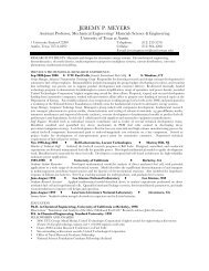
ME 360/390 – Pr<strong>of</strong>. R.G. Longoria<br />
Vehicle System Dynamics and Control<br />
Pr<strong>of</strong>. R.G. Longoria<br />
Spring 2012<br />
<strong>Department</strong> <strong>of</strong> <strong>Mechanical</strong> Engineering<br />
The University <strong>of</strong> Texas at Austin
• <strong>Steering</strong> mechanisms<br />
ME 360/390 – Pr<strong>of</strong>. R.G. Longoria<br />
Vehicle System Dynamics and Control<br />
Overview<br />
• Differentially-steered vehicle – kinematic<br />
• Ackermann steered vehicle – kinematic<br />
• Simulation examples<br />
<strong>Department</strong> <strong>of</strong> <strong>Mechanical</strong> Engineering<br />
The University <strong>of</strong> Texas at Austin
Classical steering mechanisms<br />
δ =<br />
H<br />
5 th wheel<br />
steering<br />
'hand wheel' angle<br />
‘turntable steering’<br />
•Likely developed by the Romans, and preceded only by a 2<br />
wheel cart.<br />
•Consumes space<br />
•Poor performance – unstable<br />
•Longitudinal disturbance forces have large moment arms<br />
ME 360/390 – Pr<strong>of</strong>. R.G. Longoria<br />
Vehicle System Dynamics and Control<br />
•Articulated-vehicle steering<br />
•Tractors, heavy industrial<br />
vehicles<br />
<strong>Department</strong> <strong>of</strong> <strong>Mechanical</strong> Engineering<br />
The University <strong>of</strong> Texas at Austin
Common <strong>Steering</strong> Mechanisms<br />
Differential steer Synchro-drive Tricycle<br />
What is minimum<br />
# <strong>of</strong> actuators?<br />
ME 360/390 – Pr<strong>of</strong>. R.G. Longoria<br />
Vehicle System Dynamics and Control<br />
…and some systems also employ Ackermann-type.<br />
<strong>Department</strong> <strong>of</strong> <strong>Mechanical</strong> Engineering<br />
The University <strong>of</strong> Texas at Austin
Kinematic model <strong>of</strong> single-axle turning vehicle<br />
Y<br />
Recall the simple 2D turning vehicle with kinematic state quantified by,<br />
y<br />
ME 360/390 – Pr<strong>of</strong>. R.G. Longoria<br />
Vehicle System Dynamics and Control<br />
x<br />
ψ<br />
X<br />
X<br />
[ ] †<br />
qI<br />
= X Y ψ<br />
The velocities in the local (body-fixed) reference frame<br />
are transformed into a global frame by the rotation<br />
matrix,<br />
⎡ cosψ sinψ 0⎤<br />
R(<br />
ψ ) =<br />
⎢<br />
−sinψ<br />
cosψ 0<br />
⎥<br />
⎢ ⎥<br />
⎢⎣ 0 0 1⎥⎦<br />
and the velocities are then,<br />
Inverting, we arrive at the velocities in the global reference frame,<br />
qɺ = R( ψ ) ⋅qɺ<br />
I<br />
qɺ = Ψ( ψ ) ⋅qɺ<br />
where,<br />
⎡cosψ −sinψ<br />
0⎤<br />
Ψ(<br />
ψ ) =<br />
⎢<br />
sinψ cosψ 0<br />
⎥<br />
⎢ ⎥<br />
⎢⎣ 0 0 1⎥⎦<br />
Let’s apply these relations to the case <strong>of</strong> a single-axis vehicle that has two wheels<br />
differentially driven with controlled speed.<br />
<strong>Department</strong> <strong>of</strong> <strong>Mechanical</strong> Engineering<br />
The University <strong>of</strong> Texas at Austin<br />
I
Y<br />
Recall: position and velocity in inertial frame<br />
We defined the vehicle’s kinematic state in the inertial frame by,<br />
l2<br />
y<br />
B<br />
l1<br />
x<br />
ψ<br />
So, for our simple (single-axle) vehicle,<br />
the velocities in the inertial frame in<br />
terms <strong>of</strong> the wheel velocities are,<br />
ME 360/390 – Pr<strong>of</strong>. R.G. Longoria<br />
Vehicle System Dynamics and Control<br />
X<br />
X<br />
Velocities in the local (body-fixed)<br />
reference frame are transformed<br />
into the inertial frame by the<br />
rotation matrix,<br />
or, specifically, qɺ = R( ψ ) ⋅qɺ<br />
I<br />
q<br />
I<br />
⎡ X ⎤<br />
=<br />
⎢<br />
Y<br />
⎥<br />
⎢ ⎥<br />
⎢⎣ ψ ⎥⎦<br />
⎡ cosψ sinψ 0⎤<br />
R(<br />
ψ ) =<br />
⎢<br />
−sinψ<br />
cosψ 0<br />
⎥<br />
⎢ ⎥<br />
⎢⎣ 0 0 1⎥⎦<br />
Inverting, we arrive at the velocities in the global reference<br />
frame,<br />
⎡ Xɺ ⎤ ⎡U ⎤ ⎡cosψ ⎢ ⎥<br />
qɺ I = Yɺ ⎢<br />
V<br />
⎥<br />
( ψ )<br />
⎢<br />
⎢ ⎥ =<br />
⎢ ⎥<br />
= Ψ ⋅ qɺ<br />
=<br />
⎢<br />
sinψ ⎢ψ ⎥<br />
⎣<br />
ɺ<br />
⎦<br />
⎢⎣ Ω⎥⎦<br />
⎢⎣ 0<br />
−sinψ<br />
cosψ 0<br />
0⎤<br />
⎡ vx<br />
⎤<br />
0<br />
⎥ ⎢<br />
v<br />
⎥<br />
⎥ ⎢ y ⎥<br />
1⎥⎦<br />
⎢⎣ ω ⎥ z ⎦<br />
qɺ<br />
I<br />
⎡ Rw l2Rw ⎤<br />
⎢ ( ω1 + ω2)cos ψ − ( ω1 −ω2<br />
)sinψ<br />
2<br />
B<br />
⎥<br />
⎡Xɺ ⎤ ⎢ ⎥<br />
⎢ ⎥ Rw l2Rw = Yɺ<br />
⎢ ( ω1 ω2)sin ψ ( ω1 ω2)cos ψ ⎥<br />
⎢ ⎥ = + + −<br />
⎢ 2<br />
B<br />
⎥<br />
⎢ψ ⎥<br />
⎣<br />
ɺ<br />
⎦ ⎢ ⎥<br />
⎢<br />
Rw<br />
( ω1 −ω2<br />
)<br />
⎥<br />
⎢⎣ B<br />
⎥⎦<br />
<strong>Department</strong> <strong>of</strong> <strong>Mechanical</strong> Engineering<br />
The University <strong>of</strong> Texas at Austin
Example: Differentially-driven basic vehicle<br />
For a kinematic model <strong>of</strong> a differentially-driven vehicle, we assume there is no slip, and<br />
that the wheels have controllable speeds, ω 1 and ω 2 . If the CG is on the rear axle,<br />
the velocities in the global reference frame are,<br />
ME 360/390 – Pr<strong>of</strong>. R.G. Longoria<br />
Vehicle System Dynamics and Control<br />
Y<br />
y<br />
X<br />
x<br />
ψ<br />
B = track width<br />
qɺ<br />
I<br />
l = L<br />
l<br />
1<br />
2<br />
=<br />
0<br />
⎡ Rw<br />
⎤<br />
⎢ ( ω1 + ω2) cosψ<br />
2<br />
⎥<br />
⎡Xɺ ⎤ ⎢ ⎥<br />
⎢ ⎥ Rw<br />
= Yɺ<br />
⎢ ( ω1 ω2)sin ψ ⎥<br />
⎢ ⎥ = +<br />
⎢ 2<br />
⎥<br />
⎢ψ ⎥<br />
⎣<br />
ɺ<br />
⎦ ⎢ ⎥<br />
⎢<br />
Rw<br />
( ω1 −ω2<br />
) ⎥<br />
⎢⎣ B<br />
⎥⎦<br />
<strong>Department</strong> <strong>of</strong> <strong>Mechanical</strong> Engineering<br />
The University <strong>of</strong> Texas at Austin
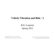
Simulation <strong>of</strong> the differentially-steered single-axle vehicle trajectory<br />
A simple code in Matlab to compute and plot out the vehicle trajectory is given below.<br />
% Differentially-steered kinematic vehicle model<br />
% Requires right (#1) and left (#2) wheel velocities, omegaw1 and omegaw2,<br />
% as controlled inputs for single axle, to be passed as global parameters<br />
% Wheel radius, R_w, and axle track width, B, are also required<br />
% Updated 2/20/12 RGL<br />
function Xidot = DS_vehicle(t,Xi)<br />
global R_w B omegaw1 omegaw2<br />
X = Xi(1); Y = Xi(2); psi = Xi(3);<br />
% NOTE: these are global coordinates<br />
% These equations assume CG on single axle<br />
Xdot = 0.5*cos(psi)*R_w*(omegaw1+omegaw2);<br />
Ydot = 0.5*sin(psi)*R_w*(omegaw1+omegaw2);<br />
psidot = R_w*(omegaw1-omegaw2)/B;<br />
Xidot=[Xdot;Ydot;psidot];<br />
% test_DS_vehicle.m<br />
clear all<br />
global R_w B omegaw1 omegaw2<br />
% Rw = wheel radius, B = track width<br />
% omegaw1 = right wheel speed<br />
R_w = 0.05; B = 0.18;<br />
omegaw1 = 4; omegaw2 = 2;<br />
Xi0=[0,0,0];<br />
[t,Xi] = ode45(@DS_vehicle,[0 10],Xi0);<br />
N = length(t);<br />
figure(1)<br />
plot(Xi(:,1),Xi(:,2)), axis([-1.0 1.0 -0.5 1.5]), axis('square')<br />
xlabel('X'), ylabel('Y')<br />
ME 360/390 – Pr<strong>of</strong>. R.G. Longoria<br />
Vehicle System Dynamics and Control<br />
Vehicle trajectory in XY<br />
<strong>Department</strong> <strong>of</strong> <strong>Mechanical</strong> Engineering<br />
The University <strong>of</strong> Texas at Austin
Simulation <strong>of</strong> differentially-steered vehicle with 2D animation<br />
A code in Matlab to plot out the vehicle trajectory including a simple graphing animation <strong>of</strong><br />
the vehicle body/orientation is provided on the course log. This provides visual feedback on<br />
the model results.<br />
The key elements <strong>of</strong> this code are:<br />
Y<br />
1.5<br />
1<br />
0.5<br />
0<br />
-0.5<br />
-1 -0.5 0<br />
X<br />
0.5 1<br />
ME 360/390 – Pr<strong>of</strong>. R.G. Longoria<br />
Vehicle System Dynamics and Control<br />
1. Specify and plot initial location<br />
and orientation <strong>of</strong> the vehicle CG.<br />
2. Initiate some ‘handle graphics’<br />
functions for defining the ‘body’.<br />
3. Perform a fixed wheel speed<br />
simulation loop to find state, q.<br />
4. The state <strong>of</strong> the robot is used to<br />
define the position and orientation<br />
<strong>of</strong> the vehicle over time.<br />
5. A simple routine is used to<br />
animate 2D motion <strong>of</strong> the vehicle<br />
by progressive plotting <strong>of</strong> the<br />
body/wheel positions.<br />
<strong>Department</strong> <strong>of</strong> <strong>Mechanical</strong> Engineering<br />
The University <strong>of</strong> Texas at Austin
Lankensperger/‘Ackermann’-type steering<br />
‘knuckle’<br />
1. <strong>Steering</strong> arm<br />
2. Drag link<br />
3. Idler arm<br />
4. Tie rod/rack<br />
5. <strong>Steering</strong> wheel<br />
6. <strong>Steering</strong> shaft<br />
7. <strong>Steering</strong> box<br />
8. Pitman arm<br />
ME 360/390 – Pr<strong>of</strong>. R.G. Longoria<br />
Vehicle System Dynamics and Control<br />
Rigid axle with<br />
kingpin<br />
Divided track rods<br />
for independent<br />
suspension.<br />
<strong>Department</strong> <strong>of</strong> <strong>Mechanical</strong> Engineering<br />
The University <strong>of</strong> Texas at Austin
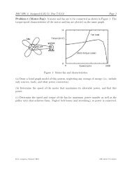
<strong>Turning</strong> at low (Ackermann) speed<br />
• What is low-speed?<br />
– Negligible centrifugal forces<br />
– Tires need not develop lateral<br />
forces<br />
• Pure rolling, no lateral sliding<br />
(minimum tire scrub).<br />
• For proper geometry in the turn,<br />
the steer angles, δ, are given by:<br />
L L<br />
δo ≅ < δi<br />
≅<br />
R + B R − B<br />
2 2<br />
• The average value (small angles)<br />
is the Ackerman angle,<br />
δ =<br />
Ackermann<br />
L<br />
R<br />
ME 360/390 – Pr<strong>of</strong>. R.G. Longoria<br />
Vehicle System Dynamics and Control<br />
L<br />
δ o<br />
B<br />
δ i<br />
R<br />
Simple relationship between<br />
heading and steering wheel angle.<br />
Ref. Wong, Ch. 5<br />
Turn Center<br />
“Ackermann steering geometry”<br />
cotδ o − cotδ<br />
i = B<br />
L<br />
δ = steer angle <strong>of</strong> outside wheel<br />
o<br />
δ = steer angle <strong>of</strong> inside wheel<br />
i<br />
B = track<br />
L = wheelbase<br />
<strong>Department</strong> <strong>of</strong> <strong>Mechanical</strong> Engineering<br />
The University <strong>of</strong> Texas at Austin
Wheel slip angle definition<br />
A positive slip angle is said to give a<br />
negative force on the wheel (to the left).<br />
Gillespie (1992)<br />
*To align the wheel with heading direction<br />
(vector), you would have to go –α.<br />
The lateral force should simply always<br />
oppose the motion – the lateral force is a<br />
dissipative force!<br />
ME 360/390 – Pr<strong>of</strong>. R.G. Longoria<br />
Vehicle System Dynamics and Control<br />
Fy = Cα ⋅α<br />
The slip angle is the angle between the<br />
wheel’s direction <strong>of</strong> heading (wheel plane)<br />
and its direction <strong>of</strong> travel. So, to compute<br />
the slip angle, need to track tire velocity<br />
components, as shown below.<br />
Excerpt from Liljedahl, et al (1996)<br />
<strong>Department</strong> <strong>of</strong> <strong>Mechanical</strong> Engineering<br />
The University <strong>of</strong> Texas at Austin
Additional notes/comments on Ackermann steering<br />
• At low speed the wheels will roll without slip angle.<br />
• If the rear wheels have no slip angle, the center <strong>of</strong> the turn lies<br />
on the projection <strong>of</strong> the rear axle. Each front steered wheel has<br />
a normal to the wheel plane that passes through the same center<br />
<strong>of</strong> the turn. This is what Ackermann geometry dictates.<br />
• Correct Ackermann reduces tire wear and is easy on terrain.<br />
• Ackermann steering geometry leads to steering torques that<br />
increase with steer angle. The driver gets feedback about the<br />
extent to which wheels are turned. With parallel steer, the trend<br />
is different, becoming negative (not desirable in a steering<br />
system – positive feedback).<br />
• Off-tracking <strong>of</strong> the rear wheels, ∆, is related to this geometry.<br />
The ‘∆’ is R[1-cos(L/R)], or approximately L 2 /(2R).<br />
ME 360/390 – Pr<strong>of</strong>. R.G. Longoria<br />
Vehicle System Dynamics and Control<br />
<strong>Department</strong> <strong>of</strong> <strong>Mechanical</strong> Engineering<br />
The University <strong>of</strong> Texas at Austin
Using the basic geometry <strong>of</strong> Ackermann steering<br />
L<br />
δ o<br />
B<br />
δ i<br />
ME 360/390 – Pr<strong>of</strong>. R.G. Longoria<br />
Vehicle System Dynamics and Control<br />
Can you pass the vehicle<br />
through a given position?<br />
1. Assume low-speed turning<br />
2. Project along rear-axle<br />
3. Define R = L/δ max<br />
4. Project from CG<br />
5. Project ideal turning path<br />
<strong>Department</strong> <strong>of</strong> <strong>Mechanical</strong> Engineering<br />
The University <strong>of</strong> Texas at Austin
Example: 2D vehicle with front-steered wheel<br />
A wheeled vehicle is said to have kinematic (or Ackermann) steering when a wheel is<br />
actually given a steer angle, δ, as shown. A kinematic model for the steered basic vehicle<br />
in the inertial frame is given by the equations,<br />
‘tricycle’<br />
Xɺ = v cosψ = Rwω<br />
cosψ<br />
Y<br />
δ<br />
Yɺ x<br />
= vsin = R sin<br />
ψ ω ψ<br />
v<br />
ψɺ = tanδ<br />
L<br />
where it is assumed that the wheels do not slip, so we<br />
can control the rotational speed and thus velocity at each<br />
wheel-ground contact.<br />
So, the input ‘control variables’ are velocity, v=R w ω,<br />
and steer angle, δ.<br />
In this example, the CG is located on the rear axle.<br />
These kinematic equations can be readily simulated.<br />
ME 360/390 – Pr<strong>of</strong>. R.G. Longoria<br />
Vehicle System Dynamics and Control<br />
w<br />
y<br />
Note:<br />
L<br />
1<br />
v = v + v<br />
2<br />
vt<br />
ωz = ψɺ<br />
=<br />
L<br />
vt<br />
tanδ<br />
=<br />
v<br />
( )<br />
1 2<br />
<strong>Department</strong> <strong>of</strong> <strong>Mechanical</strong> Engineering<br />
The University <strong>of</strong> Texas at Austin<br />
ψ<br />
L = wheel base<br />
X<br />
X
Derivation <strong>of</strong> equations<br />
Y<br />
y<br />
L<br />
ψ<br />
δ<br />
1<br />
v = v + v<br />
2<br />
( )<br />
1 2<br />
ME 360/390 – Pr<strong>of</strong>. R.G. Longoria<br />
Vehicle System Dynamics and Control<br />
x<br />
L = wheel base<br />
X<br />
X<br />
Note that the forward velocity at the front wheel<br />
is simply, v, but because <strong>of</strong> kinematic steering<br />
the velocity along the path <strong>of</strong> the wheel must be,<br />
v<br />
ωz = tanδ<br />
L<br />
v δ<br />
=<br />
v<br />
cosδ<br />
This means that the lateral velocity at the front<br />
steered wheel must be,<br />
v = vδ sinδ = v tanδ<br />
Now we can find the angular velocity about the CG, which is located at the<br />
center <strong>of</strong> the rear axle as,<br />
t<br />
<strong>Department</strong> <strong>of</strong> <strong>Mechanical</strong> Engineering<br />
The University <strong>of</strong> Texas at Austin
Example: simulation and animation <strong>of</strong> steered tricycle kinematic model<br />
% -----------------------------------------------------<br />
% tricycle_model.m<br />
% revised 2/21/12 rgl<br />
% ----------------------------------------------------function<br />
qdot = tricycle_model(t,q)<br />
global L vc delta_radc delta_max_deg R_w<br />
% L is length between the front wheel axis and rear wheel axis [m]<br />
% vc is speed command<br />
% delta_radc is the steering angle command<br />
% State variables<br />
x = q(1); y = q(2); psi = q(3);<br />
% Control variables<br />
v = vc;<br />
delta = delta_radc;<br />
% kinematic model<br />
xdot = v*cos(psi);<br />
ydot = v*sin(psi);<br />
psidot = v*tan(delta)/L;<br />
qdot = [xdot;ydot;psidot];<br />
ME 360/390 – Pr<strong>of</strong>. R.G. Longoria<br />
Vehicle System Dynamics and Control<br />
% Physical parameters <strong>of</strong> the tricycle<br />
L = 2.<strong>04</strong>0; % Length between the front wheel axis and rear wheel axis [m]<br />
B = 1.164; % Distance between the rear wheels [m]<br />
m_max_rpm = 8000; % Motor max speed [rpm]<br />
gratio = 20; % Gear ratio<br />
R_w = 13/39.37; % Radius <strong>of</strong> wheel [m]<br />
% desired turn radius<br />
R_turn = 3*L;<br />
delta_max_rad = L/R_turn; % Maximum steering angle [deg]<br />
R = 6.12 m<br />
δ = 0.33 rad = 19.1 deg<br />
<strong>Department</strong> <strong>of</strong> <strong>Mechanical</strong> Engineering<br />
The University <strong>of</strong> Texas at Austin
Summary <strong>of</strong> kinematic vehicle turning<br />
• The models introduced here provide additional review <strong>of</strong><br />
fundamental kinematics principles and how they can be applied<br />
to vehicle systems.<br />
• The concepts <strong>of</strong> differential and Ackermann steering are<br />
demonstrated through simulations.<br />
• The kinematic models are commonly used in mobile robot<br />
applications for path planning, estimation, and control.<br />
• These kinematic models cannot tell you anything about the<br />
effect <strong>of</strong> forces or stability.<br />
ME 360/390 – Pr<strong>of</strong>. R.G. Longoria<br />
Vehicle System Dynamics and Control<br />
<strong>Department</strong> <strong>of</strong> <strong>Mechanical</strong> Engineering<br />
The University <strong>of</strong> Texas at Austin
Vehicle directional stability<br />
Directional stability refers to a vehicle’s ability to<br />
stabilize its direction <strong>of</strong> motion against disturbances.<br />
So, we are typically concerned with:<br />
•Unforced transient operations (natural response)<br />
•Forced response – aperiodic inputs (step, ramp, etc.)<br />
•Forced response – periodic forcing (sine)<br />
•Steady-state directional response<br />
We’ll discuss both lateral and longitudinal stability.<br />
ME 360/390 – Pr<strong>of</strong>. R.G. Longoria<br />
Vehicle System Dynamics and Control<br />
<strong>Department</strong> <strong>of</strong> <strong>Mechanical</strong> Engineering<br />
The University <strong>of</strong> Texas at Austin
2D vehicle <strong>of</strong> Rocard<br />
ME 360/390 – Pr<strong>of</strong>. R.G. Longoria<br />
Vehicle System Dynamics and Control<br />
One <strong>of</strong> the earliest analyses <strong>of</strong> vehicle stability was<br />
conducted by Y. Rocard (1954) (Steeds, 1960).<br />
The vehicle was simplified as a rigid rectangular<br />
frame with a wheel at each corner and the plane <strong>of</strong><br />
each wheel is vertical and parallel to the frame.<br />
The steering force is assumed to be directly related to<br />
slip angle,<br />
F = Kα<br />
and the contact forces are assumed not to be affected<br />
by vehicle motion.<br />
There is no steering angle in this model.<br />
First, let’s review the lateral forces using modern<br />
notation.<br />
<strong>Department</strong> <strong>of</strong> <strong>Mechanical</strong> Engineering<br />
The University <strong>of</strong> Texas at Austin
Lateral tire forces induced by slip angles<br />
The slip angle, α, is derived using body-fixed variables.<br />
α δ<br />
− 1 y 1 z<br />
f = f − tan ⎜ ⎟<br />
vx<br />
α<br />
⎛ l Ω − v ⎞<br />
−1<br />
2 z y<br />
r = tan ⎜ ⎟<br />
vx<br />
⎝ ⎠<br />
ME 360/390 – Pr<strong>of</strong>. R.G. Longoria<br />
Vehicle System Dynamics and Control<br />
Wong (2001)<br />
⎛ v + l Ω ⎞<br />
⎝ ⎠<br />
From Liljedahl, et al (1996)<br />
v 1 y l<br />
− ⎛ + 1Ωz<br />
⎞<br />
− α f = tan ⎜ ⎟ −δ<br />
f<br />
⎝ vx<br />
⎠<br />
v 1 y l<br />
− ⎛ − 2Ω<br />
z ⎞<br />
− α r = tan ⎜ ⎟ −<br />
�<br />
δ r<br />
⎝ vx<br />
⎠<br />
rear steer<br />
<strong>Department</strong> <strong>of</strong> <strong>Mechanical</strong> Engineering<br />
The University <strong>of</strong> Texas at Austin
Tire cornering forces<br />
• The slip angle, α, is the angle between direction <strong>of</strong><br />
heading and direction <strong>of</strong> travel <strong>of</strong> a wheel (OA).<br />
• A lateral force, F yα , also referred to as a cornering<br />
force (camber angle <strong>of</strong> the wheel is zero), is<br />
generated at a tire-surface interface, but this may not<br />
be collinear with the applied force at the wheel<br />
center.<br />
• A torque is induced, referred to as a self-aligning<br />
torque. This torque helps a steered wheel return to<br />
its original position after a turn.<br />
• The distance between these two applied forces is<br />
called the pneumatic trail.<br />
• The self-aligning torque is given by the product <strong>of</strong><br />
the cornering force and the pneumatic trail.<br />
• For more on self-aligning moment and pneumatic<br />
trail, see Wong, Section 1.4.<br />
ME 360/390 – Pr<strong>of</strong>. R.G. Longoria<br />
Vehicle System Dynamics and Control<br />
t p<br />
Fs<br />
Fyα “…side slip is due to the<br />
lateral elasticity <strong>of</strong> the<br />
tire.”<br />
Fs<br />
Fyα Wong<br />
<strong>Department</strong> <strong>of</strong> <strong>Mechanical</strong> Engineering<br />
The University <strong>of</strong> Texas at Austin
Typical data on tire cornering forces<br />
“linear region”<br />
Fig. 1.23 from Wong<br />
ME 360/390 – Pr<strong>of</strong>. R.G. Longoria<br />
Vehicle System Dynamics and Control<br />
α<br />
Maximum cornering forces:<br />
•passenger car tires: 18 degrees<br />
•racing car tires: 6 degrees<br />
(Wong)<br />
Fig. 1.24 from Wong<br />
Ratio to normal load<br />
α<br />
Variables that impact cornering force:<br />
•Normal load<br />
•Inflation pressure<br />
•Lateral load transfer<br />
•Size<br />
<strong>Department</strong> <strong>of</strong> <strong>Mechanical</strong> Engineering<br />
The University <strong>of</strong> Texas at Austin
Cornering stiffness and coefficient<br />
• The cornering stiffness will depend on tire<br />
properties such as:<br />
– tire size and type (e.g., radial, bias-ply, etc.),<br />
– number <strong>of</strong> plies,<br />
– cord angles,<br />
– wheel width, and<br />
– tread.<br />
• Dependence on load is taken into account<br />
through the cornering coefficient,<br />
where Fz is the vertical load.<br />
ME 360/390 – Pr<strong>of</strong>. R.G. Longoria<br />
Vehicle System Dynamics and Control<br />
CC<br />
α =<br />
C<br />
α<br />
F<br />
<strong>Department</strong> <strong>of</strong> <strong>Mechanical</strong> Engineering<br />
The University <strong>of</strong> Texas at Austin<br />
z
Cornering stiffness and coefficients<br />
Cornering stiffness for car, light truck<br />
and heavy truck tires<br />
Fig. 1.27 from Wong<br />
ME 360/390 – Pr<strong>of</strong>. R.G. Longoria<br />
Vehicle System Dynamics and Control<br />
Effect <strong>of</strong> normal load<br />
on the cornering<br />
coefficient<br />
Fig. 1.28 from Wong<br />
<strong>Department</strong> <strong>of</strong> <strong>Mechanical</strong> Engineering<br />
The University <strong>of</strong> Texas at Austin
Now, Rocard’s linearized model<br />
Rocard derived two 2nd order ODEs for this<br />
problem*, and for linear approximations found<br />
the characteristic equation,<br />
( )<br />
2 2<br />
s + Rs + S s = 0<br />
2 2<br />
⎡ ⎤<br />
2 ⎛ a ⎞ ⎛ b ⎞<br />
R = ⎢K1 ⎜1+ K 2 ⎟ + 3 ⎜1+ 2 ⎟⎥<br />
MV ⎣ ⎝ k ⎠ ⎝ k ⎠⎦<br />
2<br />
4 K1K3 ( a + b) 2( K1a − K3b) S = − 2 2<br />
Mk<br />
( MkV )<br />
A critical speed<br />
is defined by:<br />
V<br />
=<br />
2 1 3<br />
c<br />
1 − 3<br />
ME 360/390 – Pr<strong>of</strong>. R.G. Longoria<br />
Vehicle System Dynamics and Control<br />
2<br />
2 K K ( a + b)<br />
M ( K a K b)<br />
*Refer to Steeds handout for details; we’ll<br />
come back to this later<br />
Stable for all speeds if:<br />
2<br />
I = Mk<br />
K b > K a<br />
3 1<br />
•choose the position <strong>of</strong> the mass center <strong>of</strong> the<br />
vehicle and the steering force characteristics for<br />
the front and rear tires<br />
•If the steering force are equal, then stability is<br />
assured if b is greater than a, or putting the CG in<br />
front <strong>of</strong> the midpoint <strong>of</strong> the wheelbase.<br />
<strong>Department</strong> <strong>of</strong> <strong>Mechanical</strong> Engineering<br />
The University <strong>of</strong> Texas at Austin
Directional Stability per Rocard<br />
Let’s match this up with modern notation:<br />
V<br />
2<br />
2<br />
2 2 K1K3 ( a + b)<br />
f α rα<br />
c = =<br />
M K1a − K3b M C f α L1 − Crα L2<br />
ME 360/390 – Pr<strong>of</strong>. R.G. Longoria<br />
Vehicle System Dynamics and Control<br />
K = C<br />
2C<br />
C L<br />
( ) ( )<br />
1<br />
K = C<br />
R factor = Cr L2 − C f L1<br />
> 0 (for stability at all speeds)<br />
α α<br />
So, only compute a critical speed if R factor is less than or equal to zero.<br />
A critical speed is defined by,<br />
3<br />
f α<br />
rα<br />
(Steeds, 1960)<br />
<strong>Department</strong> <strong>of</strong> <strong>Mechanical</strong> Engineering<br />
The University <strong>of</strong> Texas at Austin
The ‘Bicycle’ or Single-Track Model<br />
Adapted from Wong<br />
How would you add a disturbance?<br />
Need to determine the ‘external forces’.<br />
ME 360/390 – Pr<strong>of</strong>. R.G. Longoria<br />
Vehicle System Dynamics and Control<br />
•Assume: symmetric vehicle, no roll or pitch<br />
•Represent the two wheels on the front and rear<br />
axles by a single equivalent wheel.<br />
•The bicycle model will have at least three states:<br />
–forward translational momentum or velocity <strong>of</strong><br />
the CG<br />
–lateral translational momentum or velocity <strong>of</strong> the<br />
CG<br />
–yaw angular momentum or velocity about the CG<br />
Refer to Wong, Chapter 5, Eqs. 5.25 – 5.27:<br />
( ɺ ) �<br />
m vx −VyΩ z = Fxf cos( δ f ) + Fxr − Fyf<br />
sin( δ f )<br />
����� �����<br />
( ɺ )<br />
front drive rear drive lateral force effect<br />
m v + V Ω = F + F cos( δ ) + F sin( δ )<br />
y x z yr yf f xf f<br />
I Ω ɺ = l F cos( δ ) − l F + l F sin( δ )<br />
z z 1 yf f 2 yr 1 xf f<br />
<strong>Department</strong> <strong>of</strong> <strong>Mechanical</strong> Engineering<br />
The University <strong>of</strong> Texas at Austin
Z<br />
tan<br />
−1<br />
⎛ y 2 z ⎞<br />
⎜ ⎟ = δ r −α<br />
r<br />
vx<br />
α r<br />
Y<br />
ME 360/390 – Pr<strong>of</strong>. R.G. Longoria<br />
Vehicle System Dynamics and Control<br />
x t<br />
v − l Ω<br />
⎝ ⎠<br />
l 2<br />
vy<br />
l 1<br />
y<br />
y t<br />
A more general ‘bicycle’ model schematic<br />
ωz<br />
x<br />
β<br />
vx<br />
α f δf<br />
<strong>Department</strong> <strong>of</strong> <strong>Mechanical</strong> Engineering<br />
The University <strong>of</strong> Texas at Austin<br />
X<br />
v −1 ⎛ y ⎞<br />
β = sideslip = tan ⎜ ⎟<br />
⎝ vx<br />
⎠<br />
tan<br />
ψ<br />
v + l Ω<br />
− 1 ⎛ y 1 z ⎞<br />
⎜ ⎟ = δ f −α<br />
f<br />
vx<br />
⎝ ⎠
Reduced bicycle model: 2 DOF by assuming V x = constant = V<br />
ME 360/390 – Pr<strong>of</strong>. R.G. Longoria<br />
Vehicle System Dynamics and Control<br />
v = V<br />
x<br />
δ = δ = small steering angle<br />
f<br />
( ɺ ) �<br />
m vx −VyΩ z = Fxf cos( δ f ) + Fxr − Fyf<br />
sin( δ f )<br />
����� �����<br />
mvɺ = F + F + F δ − mv Ω<br />
y yr yf xf f x z �<br />
∼0<br />
I zΩ ɺ<br />
z = l1Fyf − l2Fyr + l1Fxf δ f<br />
���<br />
Note how δ falls out, but it enters again in the lateral forces, since,<br />
v 1 y l1 z vy l<br />
− ⎛ + Ω ⎞ ⎛ + 1Ωz<br />
⎞<br />
α f = δ f − tan ⎜ ⎟ ≈ δ f − ⎜ ⎟<br />
⎝ vx ⎠ ⎝ vx<br />
⎠<br />
front drive rear drive lateral force effect<br />
∼0<br />
l 1 2Ω z − vy l2Ω z − v<br />
− y<br />
⎛ ⎞ ⎛ ⎞<br />
αr<br />
= tan ⎜ ⎟ ≈ ⎜ ⎟<br />
⎝ vx ⎠ ⎝ vx<br />
⎠<br />
<strong>Department</strong> <strong>of</strong> <strong>Mechanical</strong> Engineering<br />
The University <strong>of</strong> Texas at Austin
As before, we can calculate vehicle trajectory calculations<br />
Recall, these models solve for forward and lateral velocity and yaw<br />
velocity, resulting from input steer angles, δ, relative to the bodyfixed<br />
axes.<br />
To find the trajectory <strong>of</strong> the CG in the Earth-based coordinates, we<br />
use transformation equations for basic 2-D trajectory simulations,<br />
ME 360/390 – Pr<strong>of</strong>. R.G. Longoria<br />
Vehicle System Dynamics and Control<br />
Xɺ = v cos( ψ ) − v sin( ψ )<br />
x y<br />
Yɺ = v sin( ψ ) + v cos( ψ )<br />
ψɺ<br />
= Ω<br />
x y<br />
z<br />
<strong>Department</strong> <strong>of</strong> <strong>Mechanical</strong> Engineering<br />
The University <strong>of</strong> Texas at Austin
Example: directional stability with zero steer + disturbance<br />
• We examine directional stability, reviewing Steeds’ form <strong>of</strong><br />
Rocard’s (linearized) model (see class handout), which is<br />
essentially the bicycle model with steer angle, δ = 0.<br />
• Determine if this vehicle with baseline parameter data given<br />
(next slide) is stable, and compare with results from a<br />
simulation <strong>of</strong> the bicycle model subjected to a force<br />
‘perturbation’ at the front wheel applied in the +y direction.<br />
• Additional ‘car specification’ data is provided as Appendix B.<br />
ME 360/390 – Pr<strong>of</strong>. R.G. Longoria<br />
Vehicle System Dynamics and Control<br />
<strong>Department</strong> <strong>of</strong> <strong>Mechanical</strong> Engineering<br />
The University <strong>of</strong> Texas at Austin
Example: baseline vehicle parameter data (from simple_bicycle.m)<br />
(In Matlab script form)<br />
% Baseline values<br />
g = 9.81;<br />
L = 3.075; L1 = 1.568; L2 = L-L1;<br />
% Inertia parameters<br />
m = 1945; % total mass, kg<br />
W = m*g; % weight, N<br />
iyaw = 0.992; % yaw dynamic index<br />
% the following is a defined relation between yaw dynamic index and<br />
% the yaw moment <strong>of</strong> inertia (see Dixon reference and table <strong>of</strong> car specs)<br />
Iz = iyaw*m*L1*L2; % moment <strong>of</strong> inertia about z, kg-m^2<br />
Wf = L2*W/L; % static weight on front axle<br />
Wr = L1*W/L; % static weight on rear axle<br />
% Refer to Wong, Section 1.4 for guide to the following parameters<br />
CCf = 0.171*180/pi; % front corning stiffness coefficient, /rad<br />
CCr = 0.5*0.181*180/pi; % rear corning stiffness coefficient, /rad<br />
Cf = CCf*Wf/2; % corning stiffness per tire, N/rad (front)<br />
Cr = CCr*Wr/2; % rear cornering stiffness per tire, N/rad (rear)<br />
ME 360/390 – Pr<strong>of</strong>. R.G. Longoria<br />
Vehicle System Dynamics and Control<br />
<strong>Department</strong> <strong>of</strong> <strong>Mechanical</strong> Engineering<br />
The University <strong>of</strong> Texas at Austin
Disturbance force application<br />
if (t>=tdon & t
For Nominal Case, Vehicle Stabilizes<br />
Given case:<br />
R factor = 4200.4<br />
V c = non-existent<br />
v x =V= 5L/sec<br />
A lateral pulse disturbance is<br />
applied at front wheel.<br />
Afterwards, the vehicle<br />
stabilizes (lateral and yaw<br />
velocities go to zero).<br />
ME 360/390 – Pr<strong>of</strong>. R.G. Longoria<br />
Vehicle System Dynamics and Control<br />
4 x 10⁻³ Lateral Velocity<br />
2<br />
0<br />
-2<br />
-4<br />
-6<br />
0 5 10 15<br />
50<br />
0<br />
-50<br />
Position<br />
0 50 100 150 200<br />
6 x 10⁻³ Yaw Velocity<br />
4<br />
2<br />
0<br />
-2<br />
0 5 10 15<br />
x 10-3 Yaw<br />
3<br />
2<br />
1<br />
0<br />
0 5 10 15<br />
Used: simple_bicycle.m<br />
<strong>Department</strong> <strong>of</strong> <strong>Mechanical</strong> Engineering<br />
The University <strong>of</strong> Texas at Austin
Change rear ‘lateral stiffness’ (i.e., the cornering stiffness values <strong>of</strong> tires)<br />
In this case, the rear lateral<br />
stiffness was cut in half.<br />
R factor = −33814.<br />
V c = 18.2 m/s<br />
Let (since vehicle is now<br />
unstable for V > Vc)<br />
V = 1.2* V c =21.8<br />
After the pulse disturbance,<br />
the vehicle does not stabilize.<br />
ME 360/390 – Pr<strong>of</strong>. R.G. Longoria<br />
Vehicle System Dynamics and Control<br />
50<br />
0<br />
-50<br />
Lateral Velocity<br />
-100<br />
0 5 10 15<br />
100<br />
50<br />
0<br />
-50<br />
Position<br />
0 100 200<br />
15<br />
10<br />
5<br />
Yaw Velocity<br />
0<br />
0 5 10 15<br />
15<br />
10<br />
5<br />
Yaw<br />
0<br />
0 5 10 15<br />
Used: simple_bicycle.m<br />
<strong>Department</strong> <strong>of</strong> <strong>Mechanical</strong> Engineering<br />
The University <strong>of</strong> Texas at Austin
Example: a double lane change using simple bicycle model<br />
Using the stable case for the<br />
‘simple_bicycle’ model, an<br />
‘open loop’ lane change is<br />
achieved by:<br />
(put right into function file):<br />
% double lane change<br />
if (t=1 & t=2 & t=3 & t=4 & t=5 & t=6) deltaf = 0; end;<br />
ME 360/390 – Pr<strong>of</strong>. R.G. Longoria<br />
Vehicle System Dynamics and Control<br />
1<br />
0.5<br />
0<br />
-0.5<br />
Lateral Velocity<br />
-1<br />
0 2 4 6 8<br />
6<br />
4<br />
2<br />
0<br />
Position<br />
-2<br />
0 50 100 150<br />
0.4<br />
0.2<br />
0<br />
-0.2<br />
Yaw Velocity<br />
-0.4<br />
0 2 4 6 8<br />
0.4<br />
0.2<br />
0<br />
-0.2<br />
Yaw<br />
-0.4<br />
0 2 4 6 8<br />
Used: simple_bicycle_lanechange.m<br />
<strong>Department</strong> <strong>of</strong> <strong>Mechanical</strong> Engineering<br />
The University <strong>of</strong> Texas at Austin
Bicycle model summary<br />
• The classic bicycle (or single-track) model forms the basis for<br />
understanding steering and steering control.<br />
• Lateral forces induced by tires depend on wheel slip angle and<br />
play a key role in lateral stability. See also the Rocard handout.<br />
• We saw earlier that longitudinal traction (driving or braking)<br />
influences lateral forces, so driven bicycle models (where there<br />
are traction/braking forces) require us to model the coupling<br />
between longitudinal and lateral tire forces (friction ellipse).<br />
• In extreme maneuvers, for example, it would be possible to<br />
predict yaw instability if lateral forces were significantly<br />
reduced.<br />
ME 360/390 – Pr<strong>of</strong>. R.G. Longoria<br />
Vehicle System Dynamics and Control<br />
<strong>Department</strong> <strong>of</strong> <strong>Mechanical</strong> Engineering<br />
The University <strong>of</strong> Texas at Austin
ME 360/390 – Pr<strong>of</strong>. R.G. Longoria<br />
Vehicle System Dynamics and Control<br />
References<br />
1. Den Hartog, J.P., Mechanics, Dover edition.<br />
2. Dixon, J.C., Tires, Suspension and Handling (2nd ed.), SAE, Warrendale, PA,<br />
1996.<br />
3. Greenwood, D.T., Principles <strong>of</strong> Dynamics, Prentice-Hall, 1965.<br />
4. Gillespie, T.D., Fundamentals <strong>of</strong> Vehicle Dynamics, SAE, Warrendale, PA, 1992.<br />
5. Hibbeler, Engineering Mechanics: Dynamics, 9th ed., Prentice-Hall.<br />
6. Meriam, J.L. and L.G. Kraige, Engineering Mechanics: Dynamics (4th ed.), Wiley<br />
and Sons, Inc., NY, 1997.<br />
7. Rocard, Y., “L’instabilite en Mecanique”, Masson et Cie, Paris, 1954.<br />
8. Segel, L., “Theoretical Prediction and Experimental Substantiation <strong>of</strong> the<br />
Response <strong>of</strong> the Automobile to <strong>Steering</strong> Control,” The Institution <strong>of</strong> <strong>Mechanical</strong><br />
Engineers, Proceedings <strong>of</strong> the Automobile Division, No. 7, pp. 310-330, 1956-7.<br />
9. Steeds, W., Mechanics <strong>of</strong> Road <strong>Vehicles</strong>, Iliffe and Sons, Ltd., London, 1960.<br />
10. Wong, J.Y., Theory <strong>of</strong> Ground <strong>Vehicles</strong>, John Wiley and Sons, Inc., New York,<br />
2001 (3rd ed.).<br />
<strong>Department</strong> <strong>of</strong> <strong>Mechanical</strong> Engineering<br />
The University <strong>of</strong> Texas at Austin
ME 360/390 – Pr<strong>of</strong>. R.G. Longoria<br />
Vehicle System Dynamics and Control<br />
APPENDIX<br />
Example Car Specifications*<br />
*Table C.1 from J.C. Dixon, “Tires, Suspension and Handling” (2 nd ed.), SAE, Warrendale, PA, 1996.<br />
<strong>Department</strong> <strong>of</strong> <strong>Mechanical</strong> Engineering<br />
The University <strong>of</strong> Texas at Austin
ME 360/390 – Pr<strong>of</strong>. R.G. Longoria<br />
Vehicle System Dynamics and Control<br />
Appendix:<br />
More on <strong>Steering</strong> Mechanisms<br />
<strong>Department</strong> <strong>of</strong> <strong>Mechanical</strong> Engineering<br />
The University <strong>of</strong> Texas at Austin
DaNI: 4-wheeled, differentially driven<br />
•Motor: Tetrix DC (handout)<br />
•Gear Ratio: 2:1<br />
•Shaft Diameter: 4.73 mm<br />
•Wheel Diameter: 100 mm<br />
•Wheel base: 133 mm.<br />
ME 360/390 – Pr<strong>of</strong>. R.G. Longoria<br />
Vehicle System Dynamics and Control<br />
Under what conditions would you need to<br />
use a dynamic model?<br />
<strong>Department</strong> <strong>of</strong> <strong>Mechanical</strong> Engineering<br />
The University <strong>of</strong> Texas at Austin
General <strong>Steering</strong> System Requirements<br />
• A steering system should be insensitive to disturbances from the ground/road<br />
while providing the driver/controller with essential ‘feedback’ as needed to<br />
maintain stability.<br />
• The steering system should achieve the required turning geometry. For<br />
example, it may be required to satisfy the Ackermann condition.<br />
• The vehicle should be responsive to steering corrections.<br />
• The orientation <strong>of</strong> the steered wheels with respect to the vehicle should be<br />
maintained in a stable fashion. For example, passenger vehicles require that<br />
the steered wheels automatically return to a straight-ahead stable equilibrium<br />
position.<br />
• It should be possible to achieve reasonable handling without excessive<br />
control input (e.g., a minimum <strong>of</strong> steering wheel turns from one locked<br />
position to the other).<br />
ME 360/390 – Pr<strong>of</strong>. R.G. Longoria<br />
Vehicle System Dynamics and Control<br />
<strong>Department</strong> <strong>of</strong> <strong>Mechanical</strong> Engineering<br />
The University <strong>of</strong> Texas at Austin
Passenger <strong>Steering</strong> Requirements<br />
• Driver should alter steering wheel angle to keep deviation from course low.<br />
• Correlation between steering wheel and driving direction is not linear due to:<br />
a) turns <strong>of</strong> the steering wheel, b) steered wheel alterations, c) lateral tire<br />
loads, and d) alteration <strong>of</strong> driving direction.<br />
• Driver must steer to account for compliance in steering system, chassis, etc.,<br />
as well as need to change directions.<br />
• Driver uses visual as well as ‘haptic’ feedback. For example, roll inclination<br />
<strong>of</strong> vehicle body, vibration, and feedback through the steering wheel (effect <strong>of</strong><br />
self-centering torque on wheels).<br />
• It is believed that the feedback from the steering torque coming back up<br />
through the steering system from the wheels is the most important<br />
information used by many drivers.<br />
ME 360/390 – Pr<strong>of</strong>. R.G. Longoria<br />
Vehicle System Dynamics and Control<br />
<strong>Department</strong> <strong>of</strong> <strong>Mechanical</strong> Engineering<br />
The University <strong>of</strong> Texas at Austin
Ref. Milliken & Milliken<br />
Impact <strong>of</strong> <strong>Steering</strong> Geometry<br />
ME 360/390 – Pr<strong>of</strong>. R.G. Longoria<br />
Vehicle System Dynamics and Control<br />
B = 0.56<br />
L<br />
Ref. Wong<br />
<strong>Department</strong> <strong>of</strong> <strong>Mechanical</strong> Engineering<br />
The University <strong>of</strong> Texas at Austin
Ref. Wong<br />
ME 360/390 – Pr<strong>of</strong>. R.G. Longoria<br />
Vehicle System Dynamics and Control<br />
<strong>Steering</strong> Results and<br />
Error in Ackermann<br />
B = 0.56<br />
L<br />
“<strong>Steering</strong> error curves” for a front beam axle<br />
<strong>Department</strong> <strong>of</strong> <strong>Mechanical</strong> Engineering<br />
The University <strong>of</strong> Texas at Austin
Impact on <strong>Steering</strong> Geometry<br />
<strong>of</strong> using Ackermann in High Speed<br />
A car with a steering geometry chosen for low-speed (Ackermann)<br />
will not be as effective at higher vehicle speeds.<br />
In a high speed turn, the inside tire will have a lower normal force,<br />
which means it could achieve the same amount <strong>of</strong> lateral cornering<br />
force with a smaller slip angle.<br />
Using Ackermann will result in more instances in which the inside<br />
tire is dragged along at too high a slip angle, unnecessarily raising<br />
the temperature and slowing the vehicle down with excessive slip<br />
induced drag.<br />
ME 360/390 – Pr<strong>of</strong>. R.G. Longoria<br />
Vehicle System Dynamics and Control<br />
<strong>Department</strong> <strong>of</strong> <strong>Mechanical</strong> Engineering<br />
The University <strong>of</strong> Texas at Austin
1. <strong>Steering</strong> arm<br />
2. Drag link<br />
3. Idler arm<br />
4. Tie rod/rack<br />
5. <strong>Steering</strong> wheel<br />
6. <strong>Steering</strong> shaft<br />
7. <strong>Steering</strong> box<br />
8. Pitman arm<br />
<strong>Steering</strong> Systems – Rigid Axle<br />
ME 360/390 – Pr<strong>of</strong>. R.G. Longoria<br />
Vehicle System Dynamics and Control<br />
Rack and pinion is not suitable for steering wheels on rigid<br />
front axles, as the axles tend to move in the longitudinal<br />
direction. This movement between the wheels and steering<br />
system can induce unintended steering action.<br />
Only steering gears (1) with rotational movement are used.<br />
Design must minimize effects from motion.<br />
7<br />
8<br />
2<br />
1<br />
You may see some older model<br />
Toyota Land Cruisers that use<br />
this type <strong>of</strong> steering design.<br />
<strong>Department</strong> <strong>of</strong> <strong>Mechanical</strong> Engineering<br />
The University <strong>of</strong> Texas at Austin
Heisler (1999)<br />
Axle-Beam <strong>Steering</strong> Linkage<br />
ME 360/390 – Pr<strong>of</strong>. R.G. Longoria<br />
Vehicle System Dynamics and Control<br />
<strong>Department</strong> <strong>of</strong> <strong>Mechanical</strong> Engineering<br />
The University <strong>of</strong> Texas at Austin
Front Axle and Tie Rod Assembly<br />
ME 360/390 – Pr<strong>of</strong>. R.G. Longoria<br />
Vehicle System Dynamics and Control<br />
From: J.W. Durstine, “The Truck <strong>Steering</strong> System From<br />
Hand Wheel to Road Wheel”, SAE, SP-374, 1973 (L. Ray<br />
Bukendale Lecture).<br />
<strong>Department</strong> <strong>of</strong> <strong>Mechanical</strong> Engineering<br />
The University <strong>of</strong> Texas at Austin
<strong>Steering</strong> Gearbox and Ratio<br />
The gearbox provides the primary means for reducing the rotational input from<br />
the steering wheel and the steering axis.<br />
<strong>Steering</strong> wheel to road wheel ratios may vary<br />
with angle, but have values <strong>of</strong> 15:1 in passenger<br />
cars and may go as high as 36:1 for heavy<br />
trucks.<br />
Rack and pinions are commonly designed to<br />
have a variable gear ratio depending on steer<br />
angle.<br />
The actual steer ratio can be influenced by<br />
steering system effects, such as compliance.<br />
The plot here from Gillespie shows how much<br />
this can change.<br />
ME 360/390 – Pr<strong>of</strong>. R.G. Longoria<br />
Vehicle System Dynamics and Control<br />
Experimentally measured steering<br />
ratio on a truck.<br />
From Gillespie (Fig. 8.18).<br />
<strong>Department</strong> <strong>of</strong> <strong>Mechanical</strong> Engineering<br />
The University <strong>of</strong> Texas at Austin
3 <strong>Steering</strong> arms<br />
7 Tie rod joints<br />
8 <strong>Steering</strong> rack<br />
ME 360/390 – Pr<strong>of</strong>. R.G. Longoria<br />
Vehicle System Dynamics and Control<br />
Rack-and-Pinion – 1<br />
Used on most passenger cars and some light trucks,<br />
as well as on some heavier and high speed vehicles.<br />
Used on vehicles with independent suspensions.<br />
<strong>Steering</strong> ratio is ratio <strong>of</strong> pinion revolutions to rack travel.<br />
Some advantages: simple, manufacturing ease,<br />
efficient, minimal backlash, tie rods can be joined<br />
to rack, minimal compliance, compact, eliminate<br />
idler arm and intermediate rod<br />
Some disadvantages: sensitive to impacts, greater<br />
stress in tie rod, since it is efficient you feel<br />
disturbances, size <strong>of</strong> steering angle depends on rack<br />
travel so you have short steering arms and higher<br />
forces throughout, cannot be used on rigid axles<br />
<strong>Department</strong> <strong>of</strong> <strong>Mechanical</strong> Engineering<br />
The University <strong>of</strong> Texas at Austin
Heisler (1999)<br />
ME 360/390 – Pr<strong>of</strong>. R.G. Longoria<br />
Vehicle System Dynamics and Control<br />
Rack-and-Pinion – 2<br />
<strong>Department</strong> <strong>of</strong> <strong>Mechanical</strong> Engineering<br />
The University <strong>of</strong> Texas at Austin
Split track-rod with relay-rod<br />
ME 360/390 – Pr<strong>of</strong>. R.G. Longoria<br />
Vehicle System Dynamics and Control<br />
Heisler (1999)<br />
<strong>Department</strong> <strong>of</strong> <strong>Mechanical</strong> Engineering<br />
The University <strong>of</strong> Texas at Austin
ME 360/390 – Pr<strong>of</strong>. R.G. Longoria<br />
Vehicle System Dynamics and Control<br />
Summary<br />
• <strong>Steering</strong> mechanisms were reviewed briefly<br />
• <strong>Steering</strong> geometry – how do you select steering<br />
system?<br />
• <strong>Steering</strong> control – how does it translate into<br />
steering mechanism design?<br />
• There is a complex relationship to suspension<br />
(see Segel, Gillespie)<br />
<strong>Department</strong> <strong>of</strong> <strong>Mechanical</strong> Engineering<br />
The University <strong>of</strong> Texas at Austin