Design and Optimization of Low-thrust Orbit Transfers - Visual and ...

Table 1. Initialandfinal orbitelements,thrustcharacteristics,spacecraft initial masses, and central bodies associated with theorbit transfers studied in this paper. The orbit elements aregivenbythesemimajoraxis(a), the eccentricity (e), inclination (i),argument of the periapsis (ω), and longitude of the ascending node (Ω). The true anomaly (θ)isleftfreeforboththeinitialand final orbit.Case Orbit a e i ω Ω Thrust Specific Initial Central(km) (degree) (degree) (degree) (N) Impulse (s) Mass (kg) BodyABCDEInitial 7000.00 0.010 0.050 0.0 0.00Target 42000.00 0.010 free free freeInitial 24505.90 0.725 7.050 0.0 0.00Target 42165.00 0.001 0.050 free freeInitial 9222.70 0.200 0.573 0.0 0.00Target 30000.00 0.700 free free freeInitial 944.64 0.015 90.060 156.9 -24.60Target 401.72 0.012 90.010 free -40.73Initial 24505.90 0.725 0.060 180.0 180.00Target 26500.00 0.700 116.000 270.0 180.001 3100 300 Earth0.350 2000 2000 Earth9.3 3100 300 Earth0.045 3045 950 Vesta2 2000 2000 Earthtransfers termed case A, B, C, D, and E. These cases correspondto those in [4], except that for case E the plane ofthe initial orbit is changed by 0.12 degrees. The gravitationalparameter for the orbit transfer around the Earth is set to be398,600.5 km 3 s −2 ,whilethatforVestais17.8km 3 s −2 .Asis customary with the classical orbit elements, values of zeroare not used for the eccentricity and inclination on accountof the singularities present in Gauss’s form of the variationalequations. The orbit transfers range from the simpler, wherefew elements have target values, to the more complex, wherenot only do all elements have target values, but also wheretemporary, large sacrificial changes must be made in someelements to change more effectively other elements, until allelements converge on their target values. Recall that to effectan orbit transfer, the Q-law not only provides thrust anglesbut also an indication of whether to thrust or coast. Thus,the Q-law can examine the trade-off between propellant massand flight time: To obtain short flight times, more propellantmust be used, while when longer flight times are allowed, therequired propellant mass is reduced. As the permitted flighttime increases, eventually there are diminishing returns onthesaved propellant mass, and so the flight time will typically becapped at some large-enough value for each of these transfers.The Pareto fronts (in propellant mass and flight time) obtainedwith the optimized Q-law are compared with those obtainedwith the nominal (unoptimized) Q-control law. Furthermore,for cases A, B, C, and D, we assess how well thePareto front of the optimized Q-law matches the performanceof individual optimal transfer trajectories reported in theliterature,computed using optimal control techniques (i.e. withoutthe imposition of a feedback control law). Due to thedifficulty of the optimal control problem, there is a dearthof optimal, many-revolution orbit transfers in the literature,especially when coast arcs are involved or when the transferis complex. For each case we present the computationtime needed to generate the Pareto front, and, where possible,compare this to the times needed to obtain the optimalsolutions reported in the literature.The nominal Q-law uses Wœ =1for orbit elements with targetvalues, Wœ =0for orbit elements without target values,and m = 3,n = 4,r = 2 for the scaling function of thesemimajor axis a. Thepenaltyfunctiontoenforceminimumperiapsis-radiusconstraints is applied only for case D and Eorbit transfers. The penalty function of the nominal Q-lawuses W p =1, k =100,andr pmin =300km for case D andr pmin =6578km for case E. The Pareto front of the nominalQ-law is acquired by varying the thrust effectivity thresholdη cut ∈ [0, 1] and the initial true anomaly θ i ∈ [0, 2π]. Inboth the nominal Q-law and the optimized Q-law, a minimumthrust-arc length of 10 degrees is imposed, measured in truelongitude (θ + ω +Ω).The GA optimization uses the following GA parameters: thepopulation size N p =1000for case A, B, C and N p =2000for case D and E, the number of generations N g =100,thepopulation replacement rate p r = 0.1, thecrossoverprobabilityp c =0.8, themutationprobabilityp m =0.3. Therelatively high mutation rate is chosen to preserve the diversityof the population. Each Q-law parameter is representedas a real-valued gene. The fitness of each individual is assignedaccording to the nondominated sorting as described inSec. 3. Possible parents are selected by tournament (i.e., randomlypick two individuals and choose the one that is betterfitted). The crossover is performed by choosing one point inthe gene string at which the two strings are crossed. The mutationis performed by randomly choosing a gene in the stringaccording to the mutation probability and resetting the generandomly within a given range.4

The SA optimization uses as its fitness function the sum ofthe consumed propellant mass and the flight time. The designof this fitness function results in an approximately equaloptimization of both the consumed propellant mass and theflight time. Thus, a complete Pareto front cannot be expectedfrom this fitness function. By replacing the flight time in thefitness function with the relative difference between the currentflight time and a specified flight time and by varying thespecified flight time, one can obtain a complete Pareto front.The SA optimization runs on a single processor, but it can betrivially parallelized by deploying N specified flight times onaclusterofNprocessors.Case A Orbit TransferCase A is a simple coplanar, circle-to-circle orbit transferfrom low Earth orbit to geostationary orbit. No periapsis constraintis imposed during the transfer, as the natural dynamicsdoes not decrease the periapsis altitude. The maximumpermittedflight time is 500 days. Figure 1 shows the Paretofront obtained with the nominal Q-law and the optimized Q-law. Note that each solution in the Pareto front for the optimalQ-law is obtained with a different set of Q-law parameters.As shown in Fig. 1, the GA Pareto front dominates the Paretofront given by the nominal Q-law.The Pareto-optimal solutions found by GA and SA are comparedwith two analytical solutions that approximately boundthe problem: The Edelbaum transfer and the Hohmann transfer.The Edelbaum transfer provides an approximate lowerlimit for the required flight time [2], while the Hohmanntransfer [13] sets an approximate lower limit for the requiredpropellant mass. The Edelbaum transfer is a continuousthrust,minimum-time transfer based on orbit averaging. TheHohmann transfer utilizes two thrust impulses, that is, two instantaneouslarge changes in velocity each without change inposition. Applying thrust impulsively is much more efficientthan applying it continuously over an orbit, and so the propellantrequired for the Hohmann transfer (assuming the thrustcan be arbitrarily large) is much less than that needed for continuousthrust. In the case of low thrust, these large velocitychanges can be accumulated gradually by utilizing a series ofsmall thrust arcs. As these thrust arcs become infinitesimal insize, the propellant requirement will converge to that neededfor the Hohmann transfer.When the Q-law optimized with GA is used, the flight-timeoptimalsolution is about 0.04 days away from the lower limitof the flight time (14.42 days), and the propellant-optimal solutionis about 0.14 kg away from the lower limit of the propellantmass (34.97 kg). In contrast, the flight-time optimalsolution found by the nominal Q-law is 0.11 days away, andthe propellant-optimal solution is 0.82 kg away. This comparisonclearly shows that the optimization of the Q-law with GAessentially matches the theoretical flight-time and propellantbounds, having improved the Pareto front of the nominal Q-law by about 0.6% in minimum flight time and about 1.9%in minimum propellant mass. The optimized-Q-law transferwith the lowest propellant mass has a flight time of about230 days, even though the maximum-permitted flight time is500 days. The distance from the flight-time cap is due to thefact that the propellant mass is already very close to its minimumvalue, and that beyond about 250 days, the flight timebecomes very sensitive to the value of η cut ,makingitdifficultto populate the Pareto front beyond this flight time.One of the limitations of the nominal Q-law for this transferis that the nominal Q-law excludes a subgroup of Paretooptimalsolutions. As shown in Fig. 1, the nominal Q-lawprovides two families of Pareto-optimal solutions: one forshort flight times (14 140). No solutions are found for the intermediateflight times (17

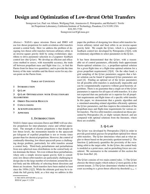
flight time is 1500 days. Figure 7 shows the trade-off betweenpropellant-mass and flight-time for this transfer. In comparisonwith the Pareto front generated with the nominal Q-law,the improvement of the Pareto front with the optimized Q-lawis dramatic. A propellant savings of about 5-15% is achievedwith the optimized Q-law. To verify the quality of the improvedPareto front, we compare it with the two optimal trajectoriesfound by Geffroy and Epenoy using an orbit averagingtechnique [14]. The inset of Fig. 7 shows that our Paretooptimalsolutions are as good as the solutions found by Geffroyand Epenoy.An analysis of the correlation between the optimal Q-lawparameters and the flight time is shown in Figure 8. Thedense populations of optimal W a around 10%, optimal W earound 20%, and W i around 70% show that the nominal Q-law (W a = W e = W i )isnotanoptimalchoice.Asexpected,the thrust effectivity threshold η cut is the important parameterto control the flight time. Other Q-law parameters (m, n, r)and the initial true anomaly (θ i )showaweakcorrelationwiththe flight time, indicating that these parameters are not as criticalas W a ,W e ,W i ,andη cut in the Q-law optimization.Case C Orbit TransferCase C is a transfer from a low-eccentricity elliptic orbitto a coplanar, high-eccentricity, larger elliptic orbit, with amaximum-permitted flight time of 20 days. Figure 9 showsthe trade-off between propellant mass and flight time forthis transfer. The Pareto front for the nominal Q-law is obtainedby varying the thrust effectivity threshold η cut ∈ [0, 1]and the initial true anomaly θ i ∈ [0, 2π]. The Pareto frontfor the GA optimized Q-law is generated by optimizing{W a ,W e ,m,n,r,η cut ,θ i }. The GA optimized Q-law providesa better estimation of the Pareto front than the nominalQ-law particularly for short flight times. For longer flighttimes, the Pareto front of the nominal Q-law is truncated ataflighttimeofabout5.3daysduetotheminimumthrustarclength constraint — when this constraint is removed, thePareto front of the nominal Q-law is improved and closelyfollows the optimized Q-law front. Several solutions foundwith the optimization tool Mystic are plotted for comparison.Mystic uses the static/dynamic control algorithm [15] [16].The comparison shows that the Pareto front generated by theoptimized Q-law is as good as the Mystic solutions.The optimal Q-law parameters found by GA are plotted withrespect to flight time in Fig. 10. The optimal W a , W e andη cut are strongly correlated to the flight time, while other Q-law parameters show a weak correlation. In general, flighttime-optimalsolutions have W e /W a > 1, whilepropellantoptimalsolutions have W e /W a < 1. This means thatthe flight-time-optimal solutions emphasize the eccentricitytarget while the propellant-optimal solutions emphasize thesemi-major axis target.Case D Orbit TransferCase D is roughly a circle-to-circle orbit transfer around theasteroid Vesta, involving a small plane change. The flighttime is capped at 300 days. Figure 11 shows the tradeoffbetween propellant mass and flight time for this transfer.The Pareto front of the nominal Q-law is obtained byvarying the thrust effectivity threshold η cut ∈ [0, 1] and theinitial true anomaly θ i ∈ [0, 2π]. The Pareto fronts of theGA optimized Q-law are generated in three different ways:the first Pareto front (GA Q-law I) is obtained by optimizing{W a ,W e ,W i ,W Ω ,η cut ,θ i },thesecondParetofront(GAQlawII) by optimizing {W a ,W e ,W i ,W Ω ,η cut ,θ i ,m,n,r},and the third Pareto front (GA Q-law III) by optimizing{W a ,W e ,W i ,η cut ,θ i ,m,n,r,W P ,r pmin ,k}. In comparisonwith the nominal Q-law, the GA optimized Q-law improvesan estimation of the Pareto front for all the flight timesconsidered. The GA optimized Q-law leads to a propellantmass savings as large as 16%. More promisingly, the Paretooptimalsolutions found with the optimized Q-law are as goodas the solution found by Whiffen using the static/dynamiccontrol algorithms coded in Mystic [16] [17].Among the three GA optimization schemes described above,GA Q-law II and GA Q-law III outperform GA Q-law I butthe difference between GA Q-law II and GA Q-law III isinsignificant. This result indicates that the trajectory doesnot depend strongly on {W P ,r pmin ,k} (the parameters ofthe penalty function for the minimum periapsis constraint)and thus an accurate Pareto front can be obtained by optimizingonly {W a ,W e ,W i ,η cut ,θ i ,m,n,r}. Thedifferencebetween the Pareto fronts generated by GA Q-law I and GAQ-law II (or III) becomes smaller as the flight time becomeslonger. This sheds some light on the effect of the Q-law parameters{m, n, r} on the Q-law performance. The parameters{m, n, r} are introduced for the scaling function in thesemimajor axis to ensure the convergence of transfers whichinvolve an increase in the semimajor axis. However, the semimajoraxis steadily decreases in this orbit transfer, suggestingthat the scaling function is not needed. Therefore, it is preferableto select a parameter set {m, n, r} that yields the smallestpossible modification to the distance function.The optimal Q-law parameters found with GA are plottedwith respect to the flight time in Figure 12. OptimalW a ,W e ,W i ,W Ω are normalized to make the sumto be 100%. The Q-law optimization shows a greatercorrelation for {W a ,W e ,W i ,W Ω ,η cut ,θ i ,m,n,r} than for{W p ,r pmin ,k}. This explains the similarity between thePareto front generated with GA Q-law II and the Pareto frontgenerated by GA Q-law III. As in other transfers, this transfershows a strong correlation between η cut and the flight time.However, the correlation does not follow the monotonoustrend that a larger η cut leads to a longer flight time. The optimalη cut shows a discontinuity around a flight time 60 days.The discontinuity also appears in other optimal Q-law parameterssuch as W a ,W e ,W Ω .Thisindicatesthatthepatternofthe trajectory changes around this flight time.8

Propellant Mass (kg)240220200180160Normal Q-lawGA optimized Q-lawSA optimized Q-lawGeffroy & Epenoyclose-up220210200190180130 140 150 160140100 200 300 400 500 600Flight Time (days)Figure 7. Case B: Trade-offbetweenpropellantmassandflight time. The Pareto fronts generated by the nominalQ-law and the GA/SA optimized Q-law are plotted incomparison with the Pareto-optimal solutions found byGeffroy and Epenoy using an orbit averaging technique.W a(%)η cutm1008060402001.00.80.60.40.20.03.02.82.62.42.22.00 200 400 600Flight Time (days)W e(%)θ i(radian)n1008060402006420109876540 200 400 600Flight Time (days)W i(%)100r80604020087654320 200 400 600Flight Time (days)Figure 8. Case B: OptimalQ-lawparametersfoundbyGAwith respect to flight time. Optimal W a ,W e ,W i arenormalized to make their sum to be 100%.Propellant Mass (kg)454035302520Normal Q-lawGA optimized Q-lawSA optimized Q-lawMystic182 3 4 5 6150 2 4 6 8 10Flight Time (days)2019close-upFigure 9. Case C: Trade-offbetweenpropellantmassandflight time. The Pareto fronts generated by the nominalQ-law and the GA/SA optimized Q-law are plotted incomparison with several Pareto-optimal solutions foundwith the optimization tool Mystic.W a(%)η cutm1008060402001.00.80.60.40.20.0201510500 2 4 6 8 10Flight Time (days)W e(%)θ i(radian)n10080604020076543210129630 2 4 6 8 10Flight Times (days)r121086420 2 4 6 8 10Flight Times (days)Figure 10. Case C: OptimalQ-lawparametersfoundbyGA with respect to flight time. A strong correlation between{W a ,W e ,η cut } and the flight time is observed, while otherQ-law parameters show a weak correlation.9

Propellant Mass (kg)4.44.24.03.83.63.43.23.02.8Normal Q-lawGA Q-law IGA Q-law IIGA Q-law IIISA Q-lawMysticclose-up3.283.243.203.1624.8 25.2 25.62.620 40 60 80 100Flight Time (days)Figure 11. CaseD:Trade-offbetweenpropellantmass and flight time. The Pareto fronts areobtained with the nominal Q-law and with theQ-law optimized with GA. A flight-time optimalsolution is found by the Q-law optimized withSA. A Pareto-optimal solution found by Mystic isalso plotted for comparison.W a (%)η cutr1001010.11.00.80.60.40.20.03.02.82.62.42.22.020 40 60 80Flight Time (days)W e(%)θ i (radian)W p1001010.17654321010 210 110 010 -110 -220 40 60 80Flight Time (days)W i (%)mr pmin (x 100 km)1001010.120.018.016.014.012.010.04.03.83.63.43.23.02.820 40 60 80Flight Time (days)W Ω (%)nk1001010.13.83.63.43.2310 310 210 110 020 40 60 80Flight Time (days)Figure 12. Case D: OptimalQ-lawparametersfoundwithGA withrespect to the flight time. The overall distribution of the optimalparameters shows that the Q-law performance is more sensitive to thechoice of {W a ,W e ,W i ,W Ω ,η cut ,θ i ,m,n,r} than {W P ,r pmin ,k}.a (km)10008006004000.4Flight Time 58 daysFlight Time 62 daysei (deg.)ω (deg.)Ω (deg.)0.20.090.490.290.089.820016012080-20-30-40-500 10 20 30 40 50 60Time (days)Figure 13. Case D:OrbitelementsasafunctionoftimeforaPareto-optimal trajectory with flight times 58 days (just below thediscontinuity point of the optimal η cut shown in Fig. 12) and 62 days (just above the discontinuity point). A large difference inthe time history of the eccentricity between the two trajectories is observed, while other orbit elements show little difference.10

To understand the cause of the discontinuity of the optimalQ-law parameters, we examine the trajectory for a flight timejust below the discontinuity point (T1) and that for a flighttime just above the discontinuity point (T2). Figure 13 showsorbit elements as a function of time during the orbit transfer.The two trajectories show a significant difference in thetime history of the eccentricity, while other orbit elements(a, i, ω, Ω)showasmalldifference.T1keepstheeccentricityclose to zero all time, but T2 shows a large increase and decreaseof the eccentricity during the orbit transfer. This trendis similar to that observed in Case A, where the circular spiraltrajectory (Edelbaum-type transfer) is flight-time optimalandthe elliptic trajectory (Hohmann-type transfer) is propellantoptimal. The two types of trajectories can be obtained withthe Q-law by either emphasizing the eccentricity target or not.This result is also observed in the distribution of the optimalW e in Figure 12. The optimal W e is greater for short-flighttimesolutions than for long-flight-time solutions.Case E Orbit TransferCase E is a transfer from a geostationary transfer orbitto a retrograde, Molniya-type orbit, involving a largeplane change. The maximum-permitted flight time is300 days. Figure 14 shows the trade-off between propellantmass and flight time for this transfer. The Pareto frontfor the nominal Q-law is obtained with varying η cut ∈[0, 1] and the initial true anomaly θ i ∈ [0, 2π]. ThreePareto fronts are generated with GA optimization as follows:the first Pareto front (GA-Q-law I) by optimizing{W a ,W e ,W i ,W ω ,W Ω }.thesecondParetofront(GAQ-lawII) by optimizing {W a ,W e ,W i ,W ω ,W Ω ,m,n,r,η cut ,θ i },and the third Pareto front (GA Q-law III) by optimizing{W a ,W e ,W i ,W ω ,W Ω ,m,n,r,η cut ,θ i ,W P ,r pmin ,k}. TheGA optimized Q-law provides a better estimation of thePareto front than the nominal Q-law for all the flight timesconsidered. A propellant mass savings as large as 30% isobtained with the GA optimized Q-law. Like Case D, GAQ-law II and GA Q-law III outperform GA Q-law I in thiscase, while the difference between GA Q-law II and III is insignificant.This result reflects the degree of influence of eachQ-law parameter on the Q-law performance. The differencebetween GA Q-law I and GA Q-law II (or III) becomes largeras the flight time increases in contrast to Case D.The optimal Q-law parameters found with GA are plottedwith respect to the flight time in Figure 15. The overall distributionof the optimal Q-law parameters shows the greater sensitivityof the Q-law performance to {W a ,W e ,W i ,W Ω ,η cut }than to {m, n, r, W p ,r pmin ,k}. The optimal η cut shows astrong correlation with flight time as was found for othertransfers. A strong preference for the relative size hierarchyW i >W Ω >W a >W ω >W e is observed for all flighttimes.Case E specifies changes in all orbit elements, making itthe most complicated transfer among the five transfers studiedhere. We examine how the change of each orbit elementinteracts with other orbit-element changes. Figure 16shows the time history of each orbit element for four differentPareto-optimal trajectories found by GA Q-law III. Forthe all four trajectories, the plane changes (i.e. i, ω, Ω) occurwhen the semimajor axis nearly reaches the maximum values,and the increase of the semimajor axis is accompanied by anincrease of the eccentricity. This behavior stems from theorbit-transfer energetics, in which the larger apoapsis radius(i.e. larger semimajor axis and larger eccentricity) reduces thecost of the plane change in terms of propellant consumption.Figure 16 also unveils a general trend in orbit-elementchanges with respect to the flight time. The trajectory withalongerflighttimeinvolvesalargerchangeofthesemimajoraxis and a later start of the plane change. For example,the shortest-flight-time trajectory (the solid line) exhibits anearly start of the plane change as the semimajor axis peaksat 50,000 km. In contrast, the longest-flight-time trajectory(the line with circles) shows almost no plane change until thesemimajor axis reaches its maximum 100,000 km. The differenceis directly related to the orbit-transfer energetics, inwhich the plane change with a larger apoapsis radius is propellantefficient. The longer flight-time trajectory takes betteradvantage of the energetics. The top panel of Fig. 16 illustratesthe time history of propellant usage during the transfer.The shortest-flight-time trajectory uses propellant withan almost constant rate. The longer-flight-time trajectoriesuse propellant with a lower rate during the first stage of thesemimajor-axis increase followed by a higher rate of propellantconsumption in the second stage of the plane change.Computational RequirementThe computation time required to obtain the Pareto front foreach orbit transfer is listed in Table 2. The computer usedfor the GA calculation is a 32 node Beowulf cluster with3.06 GHz Pentium 4 microprocessor, while the computerused for the SA calculation is a 31 node Beowulf cluster with800 MHz Pentium III microprocessor. In the GA calculation,Case C requires a relatively short computation time becausethe evaluation of each Q-law takes less time due to theshort flight time in this orbit transfer. Beside Case C, the requiredcomputation time is between 11.8 to 41.3 CPU hours.For Case A, B, and C, the GA computation evaluates 10,000sets of Q-law parameters, while for Case D and E it evaluates20,000 sets of Q-law parameters. Therefore, the time toevaluate one set of Q-law parameters (equivalently to obtainacandidatetrajectoryandtoassignitsfitness)isonlyabout0.001 CPU hours ( 0.1 minutes) on average.In addition to the efficient evaluation of candidate Q-laws/trajectories, GA and SA are amenable to a parallelcomputing implementation thanks to the independent evaluationof each candidate Q-law/trajectory in the population/ensemble.The parallel computation significantly reducesthe wall-clock time for a given computational load. Forthis work, the GA computation was performed on 10 processorsin parallel, thus requiring a wall-clock time that is one11

100100100100Propellant Mass (kg)800700600500400Normal Q-lawGA Q-law IGA Q-law IIGA Q-law IIISA Q-law3000 100 200 300 400 500Flight Time (days)W a(%)W Ω(%)r1010.11001010.187654320 200 400 600Flight Time (days)W e(%)η cutW p1010.11.00.80.60.40.20.010 110 010 -10 200 400 600Flight Time (days)W i(%)mr pmin (x 1000 km)1010.120.015.010.05.00.06.86.76.66.50 200 400 600Flight Time (days)W ω(%)nk1010.11098765410 310 210 10 200 400 600Flight Time (days)Figure 14. Case E:Trade-offbetweenpropellant mass and flight time. ThePareto fronts are obtained with thenominal Q-law and the Q-law optimizedwith GA and SA.Figure 15. Case E:OptimalQ-lawparametersfoundbyGA withrespecttoflight time. There is a strong correlation between η cut and the flight time,while other Q-law parameters show a weak correlation. A strong preferencefor the relative size hierarchy W i >W Ω >W ω >W e is observed for allflight times.M p(kg)a (10 5 km)ei (deg.)ω (deg.)Ω (deg.)60040020001.20.80.40.01.00.80.60.41501005003002502001501901801700 100 200 300 400 500Time (days)Figure 16. Case E: Consumedpropellantmassandorbitelementsasafunction of time for four Pareto-optimal trajectoriesamong the solutions found by GA Q-law III. The solid line is thetrajectorywithflighttime60days,thedashedlineisthetrajectory with flight time 156 days, the line with x symbols isthetrajectorywithflighttime275days,andthelinewithcirclesis the trajectory with flight time 482 days. As a general pattern, the trajectory with a longer flight time involves a larger changeof the semimajor axis (a)andalaterchangeoftheinclination(i)andtheargumentoftheperiapsis(ω).12

Table 2. ComputationtimesrequiredtoobtainaParetofront with the Q-law optimized with GA and SA for eachorbit transfer. SA computation was performed in a singleprocessor, while GA computation was performed on tenprocessors in parallel and thus required wall-clock time thatis one tenth the listed computation time.Orbit Transfer Computation Time (CPU hours)Case GA SAA 11.8 5.2B 13.3 22.5C 1.0 44.3D 25.8 68.9E 41.3 38.0tenth of the computation time listed in Table 2. It is the shortwall-clock time (1.2 – 4.1 hours ) that makes our optimizationmethod attractive as a guiding tool for the early stage of missiondesign where many possible scenarios need to be evaluated.It is important to note that our method produces a Paretofront (i.e., a group of Pareto-optimal solutions) within a fewhours, while other optimization algorithms tend to require asimilar amount of computational time as well as some userinteraction to acquire just a single Pareto-optimal trajectory:The Mystic solutions of Case C each typically took between6and24hourstorun(althoughonetookaboutaweek),andthe Mystic solution of Case D took about a half day [4] [16].5. CONCLUSIONSFor the design and optimization of trajectories poweredby low-thrust propulsion, we have developed an efficaciousand efficient method to obtain approximate propellantand flight-time requirements and Pareto-optimal trajectories.The method involves a two-level optimization process: i)Lyapunov-optimal thrust angles and locations are determinedwith the Q-law, ii) the Q-law is optimized with two evolutionaryalgorithms: a genetic algorithm and a simulatedannealing-relatedalgorithm. We have applied our method tofour different types of orbit transfers around the Earth and oneorbit transfer around the asteroid Vesta. The optimization ofthe Q-law yields the greatest benefit in the case of the mostcomplex of the five orbit transfers considered, although lesscomplex cases also benefit. The resulting Pareto front withthe optimized Q-law shows a propellant savings as large as30% in comparison with the nominal Q-law, and the Paretofront contains the optimal solutions found by other trajectoryoptimization algorithms.In optimization problems, there is always a trade-off betweenthe optimization quality and the computational requirement.Most of the efficient/fast optimization tools tend to yield lowqualitysolutions while high-quality optimization tools tendto require large computational resources. Both high qualityof optimization and low computational requirement areneeded in the early stages of mission design, where manypossible scenarios are considered. Our method offers boththe high optimization quality and the high computational efficiency.The trajectory quality of our method is shown to beas good as that of other state-of-the-art optimization tools.Our method yields not only a few Pareto-optimal trajectoriesbut also an accurate Pareto front for a given orbit transferwithin a few hours of computation time. The computationalefficiency arises from both the efficiency of the Q-law in obtaininga candidate trajectory and the natural parallelism ofGA/SA computation in evaluating a population/ensemble ofcandidate Q-laws/trajectories.6. ACKNOWLEDGMENTSThe authors thank Christoph Adami, Van Dang, and DidierKeymeulen for useful discussions. This work was performedat the Jet Propulsion Laboratory, California Institute of Technologyunder a contract with the National Aeronautics andSpace Administration. The research was supported by JPL’sR&TD program. This work is a part of the large effort by theJPL’s Evolvable Computation Group to develop evolutionarycomputational techniques to design and optimize complexspace systems and thus to improve on human-design of spacesystems [18].7. APPENDIXMathematically, a multi-objective optimization problem isexpressed asminimize y = {y 1 (x), ··· ,y M (x)} ∈Y, (A.1)where x = {x 1 , ··· ,x N }∈X, (A.2)and x is the N dimensional decision vector, y the M dimensionalobjective vector, X the decision space, and Y the objectivespace.Within the multi-objective optimized problem, a nondominatedsolution is the solution that is not dominated by anyother feasible solutions. The condition for the solution x a todominate x b is given by [6] [12],∀ i ∈{1, ··· ,M},y i (x a ) ≤ y i (x b )∧ ∃ i ∈{1, ··· ,M},y i (x a )

[4] A.E. Petropoulos, “Low-Thrust Orbit Transfers UsingCandidate Lyapunov Functions with a Mechanism forCoasting,” AIAA/AAS Astrodynamics Specialist Conference,AIAAPaper2004-5089,2004.[5] J.H. Holland, Adaptation in Natural and Artificial Systems,TheUniversityofMichiganPress,AnnArbor,Michigan, 1975.[6] A.H.F. Dias and J.A. de Vasconcelos, “MultiobjectiveGenetic Algorithms Applied to Solve OptimizationProblems,” IEEE Trans. Magn., 38,1133–1136,2002.[7] J.D. Schaffer, ”Multiple Objective Optimization withVector Evaluated Genetic Algorithms,” Ph.D. thesis,Vanderbilt University, 1984.[8] J. Horn, N. Nafpliotis, and D.E. Goldberg, “ A nichedpareto genetic algorithm for multiobjective optimization,”Proc. 1st IEEE Conf. Evolutionary Computation,1,82–87,1994.[9] C.M. Fonseca and P.J. Fleming, “Genetic algorithms formultiobjective optimization”, Proc. 5th Int. Conf. GeneticAlgorithms,416-423,1993.[10] Metropolis, N., Rosenbluth, A.W., Rosenbluth, M.N.,Teller, A.H., Teller, E, “Equation of State Calculationby Fast Computing Machines,” J. of Chem. Phys., 21,1087–1091, 1953.[11] Kirkpatrick, S., Gelat, C.D., Vecchi, M.P., “Optimizationby Simulated Annealing,” Science, 220, 671–680,1983.[12] N. Srinivas and K. Deb, “Multiobjective optimizationusing nondominated sorting in genetic algorithms,”Evolutionary Computation, 2,221–248,1994.[13] R.H. Battin, An Introduction to the Mathematics andMethods of Astrodynamics, 1sted.4thprinting,AIAA,New York, 1987, pp.488–489.[14] S. Geffroy and R. Epenoy, “Optimal Low-Thrust Transferswith Constraints - Generalization of AveragingTechniques,” Astronautica Acta, 41,133–149,1997.[15] G.J. Whiffen and J. A. Sims, “Application of a NovelOptimal Control Algorithm to Low-Thrust TrajectoryOptimization,” AAS/AIAA Space Flight MechanicsMeeting,AASPaper01-209,2001.[16] G.J. Whiffen, “Optimal Low-Thrust Orbit Transfersaround a Rotating Non-Spherical Body” AAS/AIAASpace Flight Mechanics Meeting, AASPaper04-264,2004.[17] In Ref. [16], solutions are sought to a different orbittransfer around Vesta than the one sought here. Althoughthe initial orbits are identical, the final orbits differ.Ref. [16] shows that the transfer being solved thereis infeasible in 25 days when Vesta is treated as a pointmass (but not when a full gravity field is included); thefinal orbit used here in Case D is the orbit reached inRef. [16] after 25 days of thrusting. This 25-day transferof Ref. [16] is an optimal transfer between the initialorbit and the orbit reached after the 25 days, and so wecompare our Case D to it.[18] R.J. Terrile, C. Adami, S.N. Chao, V.T. Dang, M.I. Ferguson,W. Fink, T.L. Huntsberger, G. Klimeck, M.A.Kordon, S. Lee, P. von Allmen, and J. Xu “EvolutionaryComputation Technologies for Space Systems,” IEEEAerospace Conference Proceedings,March2005.BIOGRAPHYSeungwon Lee is a member of technicalstaff in the Applied Cluster ComputingTechnologies Group at the JetPropulsion Laboratory. Her research interestincludes genetic algorithms, lowthrusttrajectory design, nanoelectronics,quantum computation, materialssimulation, parallel cluster computing,and advanced scientific software modernization techniques.Seungwon received her B.S. and M.S. in Physics from theSeoul National University in 1995 and 1997, and her Ph.D. inPhysics from the Ohio State University in 2002. Her dissertationfocused on the study of the electro-optical propertiesof semiconductor nanostructures. Her work is documented innumerous journals and conference proceedings.Paul von Allmen is the supervisor ofthe Applied Cluster Computing TechnologiesGroup and a senior researcherat the Jet Propulsion Laboratory. Paulis currently leading research in quantumcomputing, thermoelectric and nonlinearoptics material and device design,nano-scale chemical sensors, semiconductoroptical detectors, and low-thrust trajectory optimization.Prior to joining JPL in 2002, Paul worked at the IBMZurich Research Lab on semiconductor diode lasers, at theUniversity of Illinois on the silicon device sintering process,and at the Motorola Flat Panel Display Division as managerof the theory and simulation group and as principal scientiston micro-scale gas discharge UV lasers. Paul receivedhis Ph.D. in physics from the Swiss Federal Institute of Technologyin Lausanne, Switzerland in 1990. His work is documentedin numerous publications and patents.14

Wolfgang Fink is a Senior Researcherat NASA’s Jet Propulsion Laboratory,Pasadena, CA, Visiting Research AssistantProfessor of both Ophthalmologyand Neurological Surgery at the Universityof Southern California, Los Angeles,CA, and Visiting Associate in Physicsat the California Institute of Technology,Pasadena, CA. His research interests include theoretical andapplied physics, biomedicine, astrobiology, computationalfield geology, and autonomous planetary and space exploration.Dr. Fink obtained an M.S. degree in Physics from theUniversity of Göttingen in 1993, and a Ph.D. in TheoreticalPhysics from the University of Tübingen in 1997. His work isdocumented in numerous publications and patents.Anastassios E. Petropoulos is a SeniorMember of the Engineering Staff in theOuter Planet Mission Analysis Group atthe Jet Propulsion Laboratory. He is activelyinvolved in developing algorithmsfor designing low-thrust orbit transfers,and also in single-body and multi-bodylow-thrust mission design. In 1991 hereceived his B.S. in Aeronautical and Astronautical Engineeringfrom the Massachusetts Institute of Technology, and in1993 and 2001 he received his M.S. and Ph.D. degrees fromPurdue University. His dissertation focused on the problemof low-thrust, gravity-assist trajectory design.Richard J. Terrile created and leadsthe Evolutionary Computation Group atthe Jet Propulsion Laboratory. Hisgroup has developed genetic-algorithmbased tools to improve on human designof space systems and has demonstratedthat computer-aided design toolscan also be used for automatedinnovationand design of complex systems. He is an astronomer,the Mars Sample Return Study Scientist, the JIMO DeputyProject Scientist and the co-discoverer of the Beta Pictoriscircumstellar disk. Dr. Terrile has B.S. degrees in Physicsand Astronomy from the State University of New York at StonyBrook and an M.S. and a Ph.D. in Planetary Science from theCalifornia Institute of Technology in 1978.15