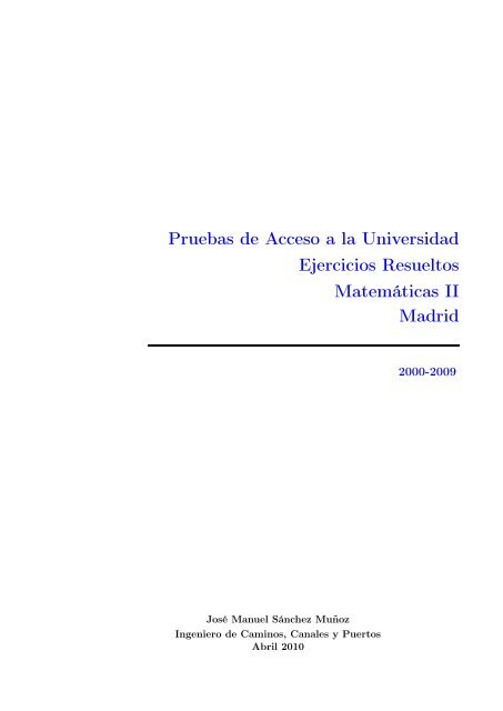
Pruebas de Acceso a la Universidad Ejercicios Resueltos ...

Pruebas de Acceso a la Universidad 

José Manuel Sánchez Muñoz 

Ejercicios Resueltos 

Ingeniero de Caminos, Canales y Puertos 

Abril 2010 

Matemáticas II 

Madrid 

2000-2009

Prólogo 

Este libro se ha hecho especialmente de los alumnos de segundo de bachillerato de la opción 

científico-tecnológica, aunque por supuesto también puede hacer uso de él cualquier estudioso de la 

materia. Se trata de la primera edición , que se ha hecho con mucho esfuerzo y con todo el cariño y 

mimo que he podido. Por supuesto que pudiera ser que encontrárais errores, por lo que os agradecería 

que me los comunicáseis para corregirlos. También agradezco de corazón la colaboración de algunos 

compañeros y compañeras de ‘Mi Rincón Matemático’ que me han ayudado enormemente con la 

recopilación de parte del material expuesto, y a su clasificación por temática. Comentar sobre este 

tema que en multitud de ocasiones en un mismo ejercicio intervienen varias temáticas. En ese caso, 

para clasificarlo he atendido (bajo un criterio propio) a que temáticas tienen más peso dentro del 

ejercicio en total, no sólo en peso de corrección, sino en peso de importancia para la resolución y 

posibilitar el continuar el ejercicio adelante. 

Si quieres hacer algún comentario, comunicar algún error o decir algo que se te ocurra, puedes 

ponerte en contacto conmigo en mirinconmatematico@gmail.com. 

Este libro se irá actualizando con los exámenes que cada año vaya poniendo la Universidad, 

pudiendo obtenerse la versión actualizada en la página: 

http://www.mates.byethost4.com. 

Este trabajo se ha hecho utilizando L ATEXy su frontend para Linux Kile (versión 2.1). Para los 

gráficos se ha usado el software de Geogebra, el de GIMP para retoque de imágenes, y el de Inkscape 

para algún gráfico vectorial de apoyo, todos ellos Open Source. Gracias a todos los que han hecho 

posible estos programas y los han compartido gratuitamente con los demás. 

He hecho una clasificación de los ejercicios por temática, esperando que la clasificación realizada 

sea del agrado de todos. 

Se trata de un trabajo que ofrezco a la comunidad educativa, pero es conveniente saber que se 

emite bajo una licencia Creative Commons en la que tienes que tener presente que: 

Tu eres libre de: 

copiar, distribuir, comunicar y ejecutar públicamente la obra. 

hacer obras derivadas. 

Bajo la siguientes condiciones: 

Atribución Debes reconocer y citar la obra de la forma especificada por el autor o el licenciante. 

No Comercial No puedes utilizar esta obra para fines comerciales. 

Licenciar Igual Si alteras o transformas esta obra, o generas una obra derivada, sólo puedes 

distribuir la obra generada bajo una licencia idéntica a ésta. 

Al reutilizar o distribuir la obra, tienes que dejar bien claro los términos de la licencia de esta 

obra. 

iii

iv 

Alguna de estas condiciones puede no aplicarse si se obtiene el permiso del titular de los 

derechos de autor.

vi 

A mi mujer Esther, 

y a mi hijo Naím. 

Sois la razón de toda mi vida y mi trabajo. 

A mis padres. 

Por haber hecho de mí, el hombre que hoy soy.

Índice general 

1. Análisis 1 

1.1. Funciones y Continuidad . . . . . . . . . . . . . . . . . . . . . . . . . . . . . . . . . . 1 

1.1.1. Junio 2000 - Ejercicio 2 - Repertorio B . . . . . . . . . . . . . . . . . . . . . . 1 



1.1.4. Septiembre 2002 - Ejercicio 2 - Repertorio A . . . . . . . . . . . . . . . . . . 4 

1.1.5. Junio 2003 - Ejercicio 2 - Repertorio A . . . . . . . . . . . . . . . . . . . . . . 4 







1.1.12. Septiembre 2007 - Ejercicio 4 - Repertorio B . . . . . . . . . . . . . . . . . . 10 





1.2. Derivadas y sus aplicaciones . . . . . . . . . . . . . . . . . . . . . . . . . . . . . . . . 13 




















vii

viii ÍNDICE GENERAL 





1.3. Integrales. Cálculo de Áreas y Volúmenes . . . . . . . . . . . . . . . . . . . . . . . . 30 







1.3.7. Junio 2009 - Ejercicio 4 - Repertorio A . . . . . . . . . . . . . . . . . . . . . . 32

Capítulo 1 

Análisis 

1.1. Funciones y Continuidad 

1.1.1. a) (1 punto) Si es posible, dibujar de forma clara la gráfica de una función 

- Solución: 

contínua en el intervalo [0,4] que tenga al menos un máximo relativo en el 

punto (2,3) y un mínimo relativo en el punto (3,4). 

b) (1 punto) Si la función fuera polinómica, ¿cuál ha de ser como mínimo su 

grado?. 

a) Veamos el croquis de la función: 

(Junio 2000) 

b) Si la función fuera polinómica, al menos debería ser de grado 3 mínimo, es decir tendría una 

expresión como esta f(x) = ax 3 + bx 2 + c x + d, ya que a priori tenemos cuatro datos que serían 

f(2) = 3, f(3) = 4, f ′ (2) = 0 y f ′ (3) = 0. 

Con esto podríamos incluso dar su expresión: 

f(x) = ax 3 +bx 2 +c x +d; f ′ (x) = 3ax 2 +2bx+c; imponiendo f(2) = 3 f(3) = 4 f ′ (2) = 0 f ′ (3) = 0 

Obtenemos: 

8a + 4b + 2c + d = 3 

27a + 9b + 3c + d = 4 

12a + 4b + c = 0 

1

2 1. Análisis 

27a + 6b + c = 0 

Obtenemos cuatro ecuaciones con cuatro incógnitas que resolviendo no darán los coeficientes 

requeridos. 

Por lo tanto: 

f(x) = −2x 3 + 15x 2 − 36x + 31 

1.1.2. Sea la función real de variable real definida por: 

- Solución: 

a) El único punto dudoso es x = 1. 

⇒ La función es contínua siempre 

b) Salvo x = 1, la derivada vale: 

f(x) = 

 

(2 − x) 3 si x ≤ 1 

x 2 si x > 1 

 

Si x → 1 − , f(x) → 1 

f(x) = 

⇒ La función no es derivable en x = 1 

Si x → 1 + , f(x) → 1 

 

−3(2 − x) 2 si x ≤ 1 

2x si x > 1 

 

Si x → 1 − , f ′ (x) → −3 

Si x → 1 + , f ′ (x) → 1 

(Junio 2001) 

c) Para obtener el área solicitada, resolvemos la integral en dos tramos. Observemos la gráfica: 

A = 

1 

0 

(8 − (2 − x) 3 )dx + 

 

= 8x + 1 

(2 − x)4 

4 

2 

(8 − x 2 )dx = 

1 

1 

+ 8x − 

0 

x3 

2 

= 

4 1 

119 

12

1.1. Funciones y Continuidad 3 

1.1.3. Se considera la función: 

- Solución: 

Se pide: 

f(x) = 

x 2 +3x+1 

x si x ≥ −1 

2x 

x−1 si x < −1 

a) (0,5 puntos) Estudiar el dominio y la continuidad de f. 

b) (1,5 puntos) Hallar las asíntotas de la gráfica de f. 

c) (1 punto) Calcular el área del recinto plano acotado limitado por la gráfica 

de f y las rectas y = 0, x = 1, x = 2. 

a) D(f) = R − {0} ya que en 0 se anula el denominador. 

(Junio 2002) 

f es contínua en los intervalos abiertos (∞, −1), (−1, 0) y (0, ∞) ya que en cada unos de ellos 

es una función cociente de funciones contínuas en las que no se anula el denominador. 

En el punto 0 la función es discontínua porque 0 /∈ D(f). 

Primera condición: 

Segunda condición: 

Tercera condición: 

f(−1) = (−1)2 + 3 · (−1) + 1 

−1 

lím f(x) = lím 

x→−1− x→−1− lím 

x→−1 + 

f(x) = lím 

x→−1 + 

= 1 

2x 

= 1 

x − 1 

x2 ⎫ 

⎪⎬ 

+ 3x + 1 

⇒ lím f(x) = 1 

⎪⎭ x→−1 

= 1 

x 

lím f(x) = f(−1) 

x→−1 

Se cumplen las tres condiciones, luego f es contínua en el punto -1. 

D(f) = R − {0} y f es contínua en el punto -1. 

b) Asíntota vertical sólo puede tener en el punto de discontinuidad, el 0. Calculamos los límites 

laterales: 

lím f(x) = lím 

x→0− x→0− x2 + 3x + 1 

lím 

x→0 + 

f(x) = lím 

x→0 + 

= −∞ 

x 

x2 ⎫ 

⎪⎬ 

⇒ La recta x = 0 es asíntota vertical. 

+ 3x + 1 ⎪⎭ = ∞ 

x 

La gráfica de f tiene tres asíntotas: x = 0, y = x + 3 e y = 2. 

c) Vemos si la gráfica de f corta al eje y = 0 en algún punto entre 1 y 2: 

x 2 + 3x + 1 

x 

Como no corta, el área pedida es: 

2 

1 

x2 + 3x + 1 

dx = 

x 

El área pedida es 5,193 u 2 . 

= 0 ⇒ x 2 + 3x + 1 = 0 ⇒ x = −3 ± √ 5 

2 

2 

1 

/∈ [1, 2] 

 

x + 3 + 1 

 

1 

dx = 

x 2 x2 2 + 3x + ln |x| = 

1 

= 1 

2 22 

1 

+ 3 · 2 + ln 2 − + 3 = 4, 5 + ln 2 = 5, 193 

2


1.1.4. Se considera la función real de variable real definida por: 

- Solución: 

f(x) = 

3 √ x − 2 si x ≥ 2 

x(x − 2) si x < 2 

a) (1 punto) Estudiar su continudad y derivabilidad. 

b) (1 punto) Hallar la ecuacióon cartesiana de la recta tangente a la gráfica 

de f en el punto (3,1). 

(Septiembre 2002) 

a) Consideramos las funciones f1(x) = x(x − 2) y f2(x) = 3√ x − 2, que forman parte de la 

definición de la función f. 

Como f1 y f2 son contínuas, f es contínua en los intervalos (−∞, 2) y (2, ∞). 

Como f1 y f2 son contínuas, f será contínua en 2 cuando f1(2) = f1(2). 

⇒ f es contínua en 2. 

Por tanto f es contínua. 

f(x) = 

 

f1(2) = 0 

f2(2) = 0 

⇒ f1(2) = f2(2) 

Como f1 es derivable y f2 es derivable en los intervalos (−∞, 2) y (2, ∞), f es derivable en los 

intervalos (−∞, 2) y (2, ∞). 

Para estudiar la derivabilidad de f en el punto 2 recurrimos a la definición de derivada y 

comenzamos por calcular la derivada por la derecha: 

f ′ (2 + ) = lím 

h→0 + 

f(2 + h) − f(2) 

= lím 

h 

h→0 + 

f2(2 + h) − 0 

= lím 

h 

h→0 + 

lím 

h→0 + 

3√ h 

h 

= lím 

h→0 + 

f es contínua. f es derivable en (−∞, 2) y (2, ∞). 

1 

3√ = ∞ ⇒ f no es derivable en 2 

h2 b) f(3) = 1, luego efectivamente el punto (3,1) pertenece a la gráfica de f. 

f2(x) = 3√ x − 2 = (x − 2) 1 

3 ⇒ f ′ 

2 = 1 

3 

La pendiente de la recta tangente vendrá dada por la derivada: 

f ′ (3) = f ′ 

2(3) = 1 

3 

2 1 

(3 − 2)− 3 = 3 

(x − 2)− 2 

3 

3√ 

2 + h − 2 

= 

h 

La ecuación punto-pendiente de la recta tangente es y − 1 = 1 

1 

3 (x − 3) ⇒ y = 3 

1.1.5. Dada la función: 

- Solución: 

f(x) = x5 − x 8 

1 − x 6 

a) (1 punto) Encontrar los puntos de discontinuidad de f. Determinar razo- 

nadamente si alguna de las discontinuidades es evitable. 

b) (1 punto) Estudiar si f tiene alguna asíntota vertical. 

(Junio 2003)


a) Podemos ver que la función es discontínua cuando el denominador se hace 0, es decir 1−x 6 = 

0 ⇒ x = −1 o x = 1. 

La discontinuidad puede evitarse si existe el límite en estos puntos. 

En x = −1 la discontinuidad no puede evitarse pues la función no posee límite en este punto. 

Veamos en x = 1: 

lím 

x→1 

x5 − x8 = 

1 − x6 lím 

x→−1 

x5 − x8 = 

1 − x6 

−2 

= ∞ 

0 

 

0 

5x 

= (L’Hôpital) = lím 

0 

x→1 

4 − 8x7 −6x5 5 − 8 1 

= = 

−6 2 

Por lo tanto como el límite existe, la discontinuidad puede evitarse, definiendo f(1) = 1 

2 . 

b) La recta x = −1 es asíntota vertical de la función pues: 

lím 

x→−1 

x5 − x8 = ∞ 

1 − x6 Además, podemos observar que si x → −1 − , f(x) → +∞; y si x → −1 + , f(X) → −∞. 

1.1.6. Calcular los siguientes límites: 

- Solución: 

a) 

a) (1,5 puntos) 

b) (1,5 puntos) 

 

lím x2 + x − x2 − x 

x→∞ 

lím 

x→∞ x [arctan(ex )] − π 

2 

2x 

lím x2 + x − x2 − x = lím √ √ = 1 

x→∞ 

x→∞ x2 + x − x2 − x 

(Junio 2003) 

b) Retocamos el límite de tal forma que obtengamos una indeterminación conocida. En este caso 

0 

0 , y a continuación aplicamos la Regla de L’Hôpital. 

lím 

x→∞ x [arctan(ex )] − π 

= lím 

2 x→∞ 

x [arctan(e x )] − π 

2 

1 

x 

= lím 

x→∞ 

e x 

1+e 2x 

− 1 

x 2 

−x 

= lím 

x→∞ 

2ex −2xe 

= lím 

1 + e2x x→∞ 

x − x2ex 2e2x −2x − x 

= lím 

x→∞ 

2 

2ex = 

−2 − 2x 

= lím 

x→∞ 2ex = lím 

x→∞ 

−2 

= 0 

2ex 1.1.7. a) (1 punto) Dibujar la gráfica de la función: 

f(x) = 2x 

x + 1 

indicando su dominio, intevalos de crecimiento y decrecimiento y asíntotas. 

b) (1 punto) Demostrar que la sucesión: 

an = 2n 

n + 1 

=


- Solución: 

es monótona creciente. 

c) (1 punto) Calcular: 

lím 

n→∞ n2 (an+1 − an) 

(Junio 2006) 

a) La función está definida para el conjunto de todos los números reales, excepto aquellos que 

hacen el denominador igual a 0, en este caso x = −1. Por lo tanto, D(f) = R − {−1}. Además 

vemos que en x=-1, la función tiene una asíntota vertical, mientras que para y = 2, la función tiene 

una asíntota horizontal. 

y = 2x 

x + 1 

y ′ = 

1 

(x + 1) 2 

Vemos que su derivada es creciente en (−∞, −1) y en (−1, +∞) 

y ′′ = 

−2 

(x + 1) 3 

Vemos que para valores del intervalo (−∞, −1), y ′′ > 0, por lo tanto la función es cóncava, y 

por el contrario en valores del intervalo (−1, +∞), y ′′ < 0, y por lo tanto la función es convexa. 

Veamos su representación: 

b) n ′ > n ⇒ 2n′ 

n ′ 2n 

+1 > n+1 

c) 

an+1 = 

por lo que f(x) es creciente para valores de x>0. 

2n + 2 

n + 2 ; an+1 

2 

− an = 

n2 ⇒ lím 

+ 3n + 2 n→∞ n2 (an+1 − an) = 2 

1.1.8. a) (1,5 puntos) Estudiar y representar gráficamente la función: 

f(x) = 

1 

(x − 2) 2 

b) (1,5 puntos) Hallar el área de la región acotada comprendida entre la 

gráfica de la función anterior y las rectas y = 1, x = 5 

2 . 

(Junio 2006)


- Solución: 

a) Claramente la función está definida para todo el conjunto de los números reales, excepto para 

el x = 2, para el que el denominador se hace 0. 

Por lo tanto el dominio de la función es D(f) = R − {0}. Claramente tiene una asíntota vertical 

en x = 2, y una asíntota horizontal en y = 0. Veamos la derivada. 

f ′ 2(x − 2) 

(x) = − 

(x − 2) 4 

Para valores del intervalo (−∞, 2), claramente f ′ (x) > 0 y por lo tanto f(x) es creciente. Para 

valores del intervalo (2, +∞), f ′ (x) < 0, y por lo tanto f(x) es decreciente. 

Veamos su representación: 

b) Para el valor de la función y = 1, obtenemos los valores de abcisa x = 1 y x = 3. Por lo tanto 

para hallar el área de la región pedida no tendremos más que hacer la integral correspondiente, eso 

sí con la precaución de ver que no podemos hacer el área mediante integración del punto asintótico. 

Por lo tanto hacemos el área, integrando f(x) desde x = 5 

2 

3 

5 

2 

hasta x = 3. 

3 1 

1 

dx = − = 1 

(x − 2) 2 x − 2 5 

2 

Obtenemos como resultado que el área solicitada es 1 u 2 . 

1.1.9. a) (1 punto) Calcular los valores de a y b para que la función: 

- Solución: 

sea contínua para todo valor de x. 

⎧ 

⎪⎨ 3x + 2 si x < 0 

f(x) = x 

⎪⎩ 

2 + 2a cos x 

ax 

si 0 ≤ x ≤ π 

2 + b si x ≥ π 

b) (1 punto) Estudiar la derivabilidad de f(x) para los valores de a y b obte- 

nidos en el apartado anterior. 


a) Para estudiar la continuidad, vemos el valor de los límites en los extremos de los intervalos e 

igualamos para obtener las incógnitas. 

lím 

x→0− f(x) = 2; lím 

x→0 + 

f(x) = 2a


Igualando ambas expresiones obtenemos que a = 2. De la misma manera: 

lím 

x→π − f(x) = π2 − 2; lím 

x→π + f(x) = π2 + b 

Igualando ambas expresiones obtenemos que b = −2. 

b) Veamos la expresión de la derivada: 

Entonces: 

f ′ ⎧ 

⎪⎨ 3 si x < 0 

(x) = 2x − 2 sin x 

⎪⎩ 

2x 

si 

si 

0 ≤ x ≤ π 

x ≥ π 

f ′ (0) = 3; f ′ (0 + ) = 0; f(x) no es derivable en x = 0 

f ′ (π − ) = 2π; f ′ (π + ) = 2π; f(x) si es derivable en x = π 

Por lo tanto f(x) es derivable en R − {0} 

1.1.10. Dibujar la gráfica de la función: 

- Solución: 

f(x) = |x| 

2 − x 

indicando su dominio, intervalos de crecimiento y decrecimiento y asíntotas. 

(2 puntos). 

Veamos la función: 

f(x) = 

 

f(x) = − x 

2−x si x < 0 

f(x) = x 

2−x si x ≥ 0, x = 2 

(Junio 2007) 

Para ver las asíntotas verticales, observamos si hay valores para los que el denominador se hace 

0. Efectivamente para x = 2 tenemos una asíntota vertical. 

Para estudiar las asíntotas horizontales, estudiamos el límite de la función cuando x → ±∞. De 

esta forma y aplicando L’Hôpital ya que tenemos indeterminaciones del tipo ∞ 

∞ , vemos que: 

modo: 

Igualmente: 

lím f(x) = −1 de este modo y = −1 es una asíntota horizontal 

x→+∞ 

lím f(x) = 1 de este modo y = 1 es una asíntota horizontal 

x→−∞ 

El estudio de crecimiento y decrecimiento lo hacemos a través de la derivada primera. De este 

f ′ (x) = − −2 

(2 − x) 2 

 

f ′ (x) < 0 

f 

si x < 0 ⇒ f es decreciente 

′ (x) > 0 si x > 0, x = 2 ⇒ f es creciente 

Veamos su representación gráfica:


1.1.11. a) (1,5 puntos) Hallar los máximos y mínimos relativos y de los puntos de 

- Solución: 

inflexión de la función: 

f(x) = 3x2 + x + 3 

x 2 + 1 

b) (1,5 puntos) Determinar una función F (x) tal que su derivada sea f(x) y 

además F (0) = 4. 


a) Para ver los máximos y mínimos relativos, hacemos el estudio de la derivada primera. 

f ′ (x) = 

1 − x2 

(x‘2 + 1) 2 

⎧ 

⎪⎨ f 

⎪⎩ 

′ (x) < 0 si x ∈ (−∞, −1) ⇒ f es decreciente 

f ′ (x) > 0 

f 

si x ∈ (−1, 1) ⇒ f es creciente 

′ (x) < 0 si x ∈ (1, +∞) ⇒ f es decreciente 

Por lo tanto en x = 1 tenemos un máximo relativo, y en x = −1 tenemos un mínimo relativo. 

Para ver los puntos de inflexión, hacemos el estudio de la derivada segunda. 

f ′′ (x) = 2x(x2 − 3) 

(x 2 + 1) 3 

Vemos que f ′′ (x) = 0 en x = − √ 3, x = 0 y x = √ 3. Por lo tanto, f ′′ (x) > 0 en el intervalo 

(−∞, − √ 3), y f(x) es cóncava. f ′′ (x) < 0 en el intervalo (− √ 3, √ 3), y f(x) es convexa. Y por 

último, f ′′ (x) > 0 en el intervalo ( √ 3, +∞), y f(x) es cóncava. 

b) 

2 3x + x + 3 

F (x) = 

x2 dx = 

+ 1 

F (0) = C = 4. Luego 

 

3 + x 

x2 

dx = 3x + 

+ 1 

1 

2 ln(x2 + 1) + C 

F (x) = 3x + 1 

2 ln(x2 + 1) + 4


1.1.12. Sea g(x) una función contínua y derivable para todo valor real de x, de la 

- Solución: 

que se conoce la siguiente información: 

i) g ′ (x) > 0 para todo x ∈ (−∞, 0) ∪ (2, +∞), mientras que g ′ (x) < 0 para todo 

x ∈ (0, 2). 

ii) g ′′ (x) > 0 para todo x ∈ (1, 3), y g ′′ (x) < 0 para todo x ∈ (−∞, 1) ∪ (3, +∞). 

iii) g(−1) = 0, g(0) = 2, y g(2) = 1. 

iv) lím g(x) = −∞, y lím g(x) = 3. 

x→−∞ x→+∞ 

Teniendo en cuenta los datos anteriores, se pide: 

a) (1 punto) Analizar razonadamente la posible existencia o no existencia 

de asíntotas verticales, horizontales u oblicuas. 

b) (1 punto) Dibujar de manera esquemática la gráfica de la función g(x). 

c) (1 punto) Si G(x) = x 

0 g(t)dt, encontrar un valor x0 tal que su derivada 

G ′ (x0) = 0. 


a) De la afirmación i) podemos asegurar que g(x) es creciente en los intervalos (−∞, 0)∪(2, +∞), 

mientras que es decreciente en el intervalo (0,2). 

De la afirmación ii) podemos asegurar que g(x) es cóncava en el intervalo (1,3), y convexa en 

los intervalos (−∞, 1) ∪ (3, +∞). 

De la afirmación iii) podemos asegurar que g(x) corta al eje de abcisas en x = −1 que punto 

de coordenadas (0,2) es un máximo relativo, y que el punto (2,1) es un mínimo relativo. Existe 

una asíntota horizontal en y = 3. No hay asíntotas verticales, y puede haber una asíntota oblícua 

cuando x → −∞. 

Veamos un croquis de la gráfica: 

c) G(x) = x 

0 g(t)dt ; G′ (x0) = g(x0) = 0 ⇔ x0 = −1 

1.1.13. Estudiar los siguientes límites: 

a) (1 punto) lím 

x→+∞ (ex − x 2 ) 

b) (1 punto) lím 

x→+∞ 

4 x + 5 x 

3 x + 6 x 

(Junio 2008)


- Solución: 

a) 

lím 

x→+∞ 

x2 = 

ex lím 

x→+∞ (ex − x 2 ) = lím 

x→+∞ ex 

 

1 − x2 

ex 

= ∞ ya que 

 

∞ 

 

∞ 

Por tanto el límite solicitado es ∞. 

b) 

lím 

x→+∞ 

aplicamos la Regla de L’Hôpital = lím 

x→+∞ 

4x + 5x 3x = lím 

+ 6x x→+∞ 

Por tanto el límite solicitado es 0. 

4 x 

6x + 5x 

6x 3x 6x + 6x 

6x = lím 

x→+∞ 

 

4 

6 

3 

6 

2x 

= lím 

ex x→+∞ 

x 

5 x 

+ 6 0 + 0 

x = = 0 

+ 1 0 + 1 

2 

= 0 

ex 1.1.14. Obtener los máximos y mínimos relativos, y los puntos de inflexión de la 

- Solución: 

función f(x) = x(ln x) 2 , siendo ln x el logaritmo neperiano de x. (2 puntos). 

Resolvemos la ecuación f ′ (x) = 0: 

f(x) = x(ln x) 2 ⇒ f ′ (x) = (ln x) 2 + x2 ln x 1 

x = (ln x)2 + 2 ln x 

f ′ (x) = 0 ⇒ (ln x) 2 + 2 ln x ⇒ ln x ln x + 2 = 0 ⇒ 

 

 

⇒ 

ln x = 0 

ln x + 2 = 0 

⇒ x = 1 

−2 ⇒ x = e 

⇒ x = 

1 

e−2 Usamdo f ′′ estudiamos las soluciones obtenidas: 

f ′ (x) = (ln x) 2 + 2 ln x ⇒ f ′′ (x) = 2 ln x 1 1 

+ 2 

x x 

f ′′ (x) > 0 ⇒ f tiene un mínimo relativo en x = 1. 

f ′′ (e −2 ) < 0 ⇒ f tiene un máximo relativo en x = e −2 

Resolvemos la ecuación f ′′ (x) = 0: 

2 

= (ln x + 1) 

x 

f ′′ (x) = 0 ⇒ 2 

(ln x + 1) = 0 ⇒ ln x + 1 = 0 ⇒ x = e−1 

x 

Usando f ′′′ estudiamos la solución obtenida: 

f ′′ (x) = 2 

x (ln x + 1) ⇒ f ′′′ (x) = − 2 

2 

(ln x + 1) + 

x2 x 

· 1 

x 

f ′′′ (e −1 ) = 0 ⇒ f tiene un punto de inflexión en x = e −1 

(Junio 2008) 

f tiene un mínimo relativo en x = 1, un máximo relativo en x = e −2 , y un punto de inflexión 

en x = e −1 . 

1.1.15. Calcular el siguiente límite: 

según los valores del parámetro a. 

 

1 

lím 1 + 

x→∞ ax2 x+1 + 4x + 8 

(Junio 2009)


- Solución: 

En primer lugar observamos que se trata de una indeterminación de la forma: 

 

1 

lím 1 + 

x→∞ ax2 x+1 = 1 

+ 4x + 8 

∞ 

independientemente del valor que tome el parámetro a. 

Recordemos que si lím f(x) = 1 y lím g(x) = ∞, entonces 

x→∞ x→∞ 

Lo cual, aplicado en nuestro límite: 

 

1 

lím 1 + 

x→∞ ax2 x+1 lím 

= e 

+ 4x + 8 

Ahora bien como: 

Entonces: 

lím 

x→∞ (f(x))g(x) = e lím g(x)(f(x) − 1) 

x→∞ 

x→∞ 

 

x + 1 

lím 

x→∞ ax2 

+ 4x + 8 

 

1 

(x + 1) 

ax2 

x + 1 

lím 

+ 4x + 8 x→∞ 

= e ax2 

+ 4x + 8 

= 

 

0 si a = 0 

1 

4 si a = 0 

 

1 

lím 1 + 

x→∞ ax2 

x+1 

1 si a = 0 

= 

+ 4x + 8 

4√ 

e si a = 0 

Como recordatorio, el límite cuando x → ∞ de: 

con a0 y b0 no nulos es a0 

b0 . 

Recordemos también que lím 

x→∞ 

del denominador, es cero. 

1.1.16. a) (1 punto) Dada la función: 

- Solución: 

a0x n + a1x n−1 + · · · + an 

b0x n + b1x n−1 + · · · + bn 

p(x) 

son tales que el grado del numerador es menor que el grado 

q(x) 

f(x) = x 

1 − x 2 

hallar el punto o los puntos de la gráfica de f(x) en los que la pendiente de 

la recta sea 1. 

b) (0,5 puntos) Hallar la ecuación de la recta tangente a la gráfica de f(x) 

en el punto x = 0. 

c) (1,5 puntos) Sea g una función derivable con derivada contínua en toda 

la recta real, y tal que g(0) = 0, g(2) = 2. Demostrar que existe al menos un 

punto c en el intervalo (0,2) tal que g ′ (c) = 1. 


a) Para resolver este apartado, tendremos que obtener la expresión de la derivada primera f ′ (x). 

f ′ (x) expresa la pendiente de la recta tangente a la curva expresada por f(x) en x. Por lo tanto 

igualando a 1 obtendremos una ecuación cuyas raices serán los puntos que cumplen la condición 

pedida.

1.2. Derivadas y sus aplicaciones 13 

Expresemos la derivada: 

f ′ (x) = (1 − x2 ) + (−2x)x 

(1 + x 2 ) 2 

= 1 − x2 − 2x2 (1 − x2 1 − 3x2 

= 

) 2 (1 − x2 ) 2 

1 − 3x 2 

(1 − x 2 ) 2 = 1 ⇒ 1 − 3x2 = 1 + x 4 − 2x 2 ⇒ x 4 + x 2 = 0 

Por lo tanto el único punto que cumple que la pendiente de su recta tangente es igual a 1 es el 

punto de coordenadas (0,0). 

b) Del anterior apartado ya tenemos la expresión de la recta tangente en x = 0. 

La ecuación de la recta tangente a f(x) en x = 0 es y = x. 

c) Para la demostración del resultado solicitado nos basamos en el Teorema del Valor Medio o 

los Incrementos Finitos para una función expresado por Joseph Louis de Lagrange 1 . Este Teorema 

es una particularidad del Teorema del Valor Medio generalizado demostrado por Augustin Louis 

Cauchy 2 a partir del Teorema de Rolle 3 . 

Cauchy demostró que dadas dos funciones f, g tal que son contínuas en un intervalo cerrado 

[a, b], y derivables en el abierto (a, b), entonces existe al menos un punto del intervalo c ∈ [a, b] tal 

que cumple la siguiente expresión [f(a) − f(b)] · g ′ (c) = [g(a) − g(b)] · f ′ (c). 

Para demostrar nuestro resultado, nos basamos en el resultado que obtuvo J.L.de Lagrange con 

su Teorema de los Incrementos Finitos para una función. Sólo es necesario expresar el resultado que 

demostró A.L. Cauchy, cogiendo como f(x) = x. De este modo, dado una función g(x), contínua en 

un intervalo cerrado [a, b], y derivable en [a, b], como en este caso es la función g(x) que nos dan en 

el enunciado, entonces, existe al menos un punto c perteneciente al intervalo [a, b] tal que se cumple: 

g ′ (c) = 

g(b) − g(a) 

b − a 

Basta expresar este resultado con los datos facilitados en el enunciado y obtenemos el resultado: 

g ′ (c) = 

g(2) − g(0) 

2 − 0 

= 2 − 0 

= 1 

2 − 0 

Al menos existirá un punto c ∈ [0, 2] tal que cumpla que g ′ (c) = 1, tal y como queríamos 

demostrar. 

1.2. Derivadas y sus aplicaciones 

1.2.1. Sea f(x) = ax 3 +bx 2 +cx+d un polinomio que cumple f(1) = 0, f ′ (0) = 2, y tiene 

- Solución: 

dos extremos relativos para x = 1 y x = 2. 

a) (2 puntos) Determinar a, b, c y d. 

b) (1 punto) ¿Son máximos o mínimos los extremos relativos? 

(Junio 2000) 

a) Para obtener los coeficientes del polinomio f(x) basta con que sustituyamos las condiciones 

que nos dan en el enunciado (cuatro ecuaciones con 4 incógnitas). Que el polinomio tiene unos 

extremos relativos en x = 1 y x = 2, es equivalente a decir que f ′ (1) = 0 y que f ′ (2) = 0. Con todo 

esto tenemos: 

1 Consultar Wikipedia: Joseph Louis de Lagrange, Teorema del Valor Medio para una función 

2 Consultar Wikipedia: Augustin Louis Cauchy 

3 Consultar Wikipedia: Teorema de Rolle


f(x) = ax 3 + bx 2 + cx + d; f ′ (x) = 3ax 2 + 2bx + c; 

f(1) = 0 ⇒ a + b + c + d = 0; f ′ (0) = 2 ⇒ c = 2; f ′ (1) = 0 ⇒ 3a + 2b + c = 0; 

Resolviendo, obtenemos: 

f ′ (2) = 0 ⇒ 12a + 4b + 2 = 0 

f(x) = 1 

3 x3 − 3 

2 x2 + 2x − 5 

6 

b)Vemos que el polinomio cumple los siguientes condicionantes: 

⎧ 

⎪⎨ [−∞, 1] → f 

⎪⎩ 

′ (x) > 0 → f(x) es creciente 

[1, 2] → f ′ (x) < 0 → f(x) es decreciente 

[2, +∞] → f ′ ⎫ 

⎪⎬ 

⎪⎭ 

(x) > 0 → f(x) es creciente 

Por lo tanto podemos afirmar que para x = 1 el polinomio tiene un máximo relativo, mientras 

que para x = 2 tiene un mínimo relativo. 

1.2.2. Sea la función f(x) = 2x − sen2x: 

- Solución: 

a) (1 punto) Determinar si tiene asíntotas de algún tipo. 

b) (1 punto) Estudiar su monotonía y la existencia de extremos relativos. 

a) Veamos la representación de la función: 

Podemos ver fácilmente que lím 

creciente. 

x→±∞ 

(Junio 2000) 

f(x) = ±∞, por lo que se trata de una función monótona 

Claramente no tiene asíntotas verticales, ni horizontales. Veamos las oblicuas: 

f(x) 2x + sin 2x 

m = lím = lím 

= 2n = lím f(x) − mx = lím 2x + sin 2x − 2x 

x→±∞ x x→±∞ x 

x→±∞ x→±∞ 

La función sin 2x está acotada entre 1 y -1, por lo tanto n = ±1.


En conclusión, tenemos que la función es monótona creciente y crece acotada entre dos rectas 

oblícuas que no son asíntotas, puesto que la función llega a tocar a estas rectas en infinitos puntos, 

ya que sin 2x es periódica de periodo 2π. 

b) Veamos los extremos relativos mediante es estudio de sus derivadas. 

f ′ (x) = 2 + 2 cos 2x; f ′ (x) = 0 ⇒ 2 + 2 cos 2x = 0 ⇒ x = π 

2 + kπ · · · k ∈ {1, 2, 3 · · · n|n ∈ N} 

Luego x = π 

2 + kπ · · · k ∈ {1, 2, 3 · · · n|n ∈ N}, son extremos relativos. 

f ′′ (x) = −4 sin 2x; f ′′ (x) = 0 ⇒ −4 sin 2x = 0 ⇒ x = π 

2 + kπ · · · k ∈ {1, 2, 3 · · · n|n ∈ N} 

Luego igualmente x = π 

2 + kπ · · · k ∈ {1, 2, 3 · · · n|n ∈ N}, son puntos de inflexión de la función. 

Vemos que para todo punto, de la función f ′′ (x) < 0, y por lo tanto f(x) es convexa en todo su 

dominio, y todos los puntos anteriormente descritos son máximos relativos a la vez que puntos de 

inflexión. 

1.2.3. Dados tres números reales cualesquiera r1, r2, r3, hallar el número real x que 

- Solución: 

a 0. 

minimiza la función: 

D(x) = (r1 − x) 2 + (r2 − x) 2 + (r3 − x) 2 

(Junio 2000) 

Para hallar el número real x que minimiza la función, bastará hallar su derivada e igualar ésta 

D ′ (x) = −2(r1 − x) − 2(r3 − x) − 2(r3 − x) ⇒ 6x − 2r1 − 2r2 − 2r3 = 0 ⇒ x = r1 + r2 + r3 

3 

1.2.4. Sea la función f(x) = x 4 − 4x 3 + x 2 + 6x. 

- Solución: 

a) (1,5 puntos) Determinar los puntos de corte de su gráfica con los ejes y los 

intervalos de crecimiento y decrecimiento. 

b) (0,5 puntos) Esbozar la gráfica de la función. 

c) (1 punto) Calcular el área determinada por la gráfica de f, el eje horizontal 

y las rectas x = −1 y x = 2. 


a) f(x) corta al eje de abcisas, cuando su ordenada se hace cero, es decir cuando f(x) = 0. 

Veamos su descomposición: 

f(x) = x(x 3 − 4x 2 + x + 6), por lo tanto x = 0 es una raiz del polinomio. 

Luego la función pasa por el origen de coordenadas (0,0). Para obtener el resto de raices, podemos 

aplicar la Regla de Rufinni: 

Así veremos que x = −1, x = 2 y x = 3, son las otras raices del polinomio. Por lo tanto la 

función corta a los ejes de coordenadas en (-1,0), (0,0), (2,0) y (3,0). 

Veamos los intervalos de crecimiento y decrecimiento, para ello hacemos el estudio de la derivada 

primera. 

f ′ (x) = 4x 3 − 12x 2 + 2x + 6;


Veamos donde se anula: 

f ′ (x) = 0 ⇒ (x − 1)(2x2 − 4x − 3) = 0 ⇒ (x − 1)(x − 1 − 1 

√ √ 

1 

2 7)(x − 1 + 2 7) = 0 

Por lo tanto x = 1 y x = 1 ± 1 

√ 

′ 

2 7, son las tres raices del polinomio de f (x), resultando: 

⎧ 

[−∞, 1 − 

⎪⎨ 

⎪⎩ 

1 

√ 

′ 

2 7] → f (x) < 0 → f(x) es decreciente 

[1 − 1 

√ 

′ 

2 7, 1] → f (x) > 0 → f(x) es creciente 

[1, 1 + 1 

⎫ 

⎪⎬ 

√ 

′ 7] → f (x) < 0 → f(x) es decreciente 

⎪⎭ 

b) Veamos la gráfica: 

c) Para hallar el área solicitada: 

0 

A = − f(x)dx + 

−1 

2 

[1 + 1 

√ 

′ 

2 7, +∞] → f (x) > 0 → f(x) es creciente 

2 

El área solicitada es 20 

3 u2 . 

0 

f(x)dx = x5 

5 − x4 + x3 

−1 

+ 3x2 + 

3 0 

x5 

5 − x4 + x3 

2 

+ 3x2 = 

3 0 

= 22 76 20 

+ = 

15 15 3 

1.2.5. a) (1 punto) Determinar los extremos relativos de la función f(x) = x 2 −4x+2. 

- Solución: 

Dibujar la gráfica. 

b) (1 punto) Hallar las ecuaciones de las dos rectas tangentes a la gráfica de 

f que pasa por el punto p(3, −5) 

a) Para el estudio de los extremos relativos, utilizamos la derivada. 

f(x) = x 2 − 4x + 2 ⇒ f ′ (x) = 2x − 4 = 0 ⇒ x = 2 

f ′′ (x) = 2 > 0. El mínimo se da en el punto (2,-2). 

La gráfica es la parábola que se adjunta en la siguiente figura. 

(Junio 2001)


b) La ecuación de la tangente será: 

Esto es, 

y − f(x0) = f ′ (x0)(x − x0) 

−5 − (x 2 0 − 4x + 2) = (2x0 − 4)(3 − x0) ⇒ x0 = 1 y x0 = 5 

Luego los puntos de tangencia son Q = (1, −1) y R = (5, 7). 

Las rectas tangentes serán: 

y + 1 = −2(x − 1) ⇒ y = −2x + 1; y y − 7 = 6(x − 5) ⇒ y = 6x − 23 

1.2.6. a) (1 punto) Calcular a y b para que las gráficas de f y g sean tangentes en 

- Solución: 

el punto de abcisa x = 2. 

b) (1 punto) Para los valores de a y b calculamos en el apartado anterior, 

dibujar las gráficas de ambas funciones y hallar la ecuación de la recta tangente 

común. 

c) (1 punto) Para los mismos valores de a y b, hallar el área limitada por las 

gráficas de las funciones el eje vertical. 

a) Debe cumplirse que f(2) = g(2) y f ′ (2) = g ′ (2). 

f(2) = 3; g(2) = 4a + b ⇒ 3 = 4a + b f ′ (x) = 2x − 2; g ′ (x) = 2ax ⇒ 2 = 4a ⇒ a = 1 

2 

Por lo tanto, g(x) = x2 

2 + 1 

b) Las gráficas son las siguientes: 


⇒ b = 1


La ecuación de la tangente común es: 

y = f(2) = f ′ (2)(x − 2) ⇒ y = 2x − 1 (es la recta tangente trazada en la figura) 

c) El área es la zona sombreada, que vale: 

A = 

2 

0 

(x 2 − 2x + 3 − 1 

2 x2 − 1)dx = 

Por lo tanto el área solicitada vale 4 

3 u2 . 

2 

0 

( 1 

2 x2 − 2x + 2)dx = 

1.2.7. Se considera la función real definida por: 

- Solución: 

f(x) = 

1 

x 2 + 3 

 

1 

6 x3 − x 2 2 + 2x = 

0 

8 4 

= 

6 3 

a)(1 punto) Hallar la ecuación cartesiana de la recta tangente en el punto de 

inflexión de abcisa positiva de la gráfica de f. 

b)(2 puntos) Calcular el área del recinto plano acotado limitado por la gráfica 

de f, la recta anterior y el eje x=0. 

(Junio 2002) 

a) Para calcular las abcisas de los puntos de inflexión igualamos a cero la derivada segunda y 

resolvemos la ecuación: 

f(x) = 

1 

x2 + 3 ⇒ f ′ 2x 

(x) = − 

(x2 + 3) 2 ⇒ f ′′ (x) = − 2(x2 + 3) 2 − 2x2(x2 + 3)2x 

(x2 + 3) 4 = 

= 8x2 − 2(x2 + 3) 

(x2 + 3) 2 = 6x2 − 6 

(x2 + 3) 3 ; f ′′ (x) = 0 ⇒ 6x 2 − 6 = 0 ⇒ x 2 

1 

= 1 ⇒ x = 

−1 

La solución x = −1 no es válida por no ser positiva, así que hay que comprobar si en x = 1 hay 

un punto de inflexión: 

f ′′′ (x) = 12x(x2 + 3) 3 − (6x 2 − 6)3(x 2 + 3) 2 2x 

(x 2 + 3) 6 

⇒ f ′′′ (1) = 0 

Luego f tiene un punto de inflexión en x = 1; el valor de la ordenada es y = f(1) = 1 

4 

La pendiente de la recta tangente es m = f ′ (1) = − 2 1 

16 = − 8 

La recta pendiente tiene ecuación t ≡ y = − 1 

4 

= − 1 

8 

(x − 1) ⇒ t ≡ y = − 1 

8 

x + 3 

8 

b) La recta t y la gráfica de f se cortan en x = 1, luego la superficie pedida es: 

1 

0 

 

= − 1 1 

· 

8 2 x2 + 3 

x − 

8 

− 1 3 1 

x + − 

8 8 x2 

dx = 

+ 3 

El área pedida es 0,01020 u 2 . 

√ 

3 

3 arctan 

 

x√3 

1 1 

0 

0 

⎛ 

⎜ 

⎝− 1 3 

x + 

8 8 − 

√ 

3 

3 · 

⎞ 

1√ 

3 ⎟ 

2 ⎠ dx = 

x√3 + 1 

= − 1 1 3 

· + 

8 2 8 − 

√ 

3 

3 arctan 

 

1 

√3 = 0, 01020 u 2 

1.2.8. Se considera la función real de variable real definida por: 

f(x) = x 

x 2 + 1


- Solución: 

a) (1 punto) Determinar sus máximos y sus mínimos relativos. 

b) (1 punto) Calcular el valor de a > 0 para el cual se verifica la igualdad 

a 

f(x)dx = 1. 

0 

a) Resolvemos la ecución f ′ (x) = 0: 

f(x) = x 

x 2 + 1 ⇒ f ′ (x) = x2 + 1 − x · 2x 

(x 2 + 1) 2 

⇒ −x 2 

1 

+ 1 = 0 ⇒ x = 

−1 

Sustituimos en la derivada segunda las soluciones obtenidas: 

= −x2 + 1 

(x2 2 = 0 ⇒ 

+ 1) 

f ′′ (x) = −2x(x2 + 1) 2 − (−x 2 + 1)2(x 2 + 1)2x 

(x 2 + 1)4 

f ′′ (−1) > 0 ⇒ f tiene un mínimo relativo en x = −1 

f ′′ (−1) < 0 ⇒ f tiene un máximo relativo en x = 1 

Calculamos las ordenadas de los puntos sustituyendo en f: 

x = −1 ⇒ y = f(−1) = −1 

1 

; x = 1 ⇒ y = f(1) = 

2 2 

f tiene un mínimo relativo en el punto (−1, −1 

1 

2 ) y un máximo relativo en (1, 2 ). 

b) Calculamos el valor de la integral definida: 

a 

0 

f(x)dx = 

a 

Resolvemos la ecuación pedida: 

a 

0 

0 

x 

x2 a 

1 2x 

dx = 

+ 1 2 0 x2 1 

dx = 

+ 1 2 ln(x2 a + 1) = 

0 

1 

2 ln(a2 + 1) 


f(x)dx = 1 ⇒ 1 

2 ln(a2 + 1) = 1 ⇒ ln(a 2 + 1) = 2 ⇒ a 2 + 1 = e 2 ⇒ a = ± e 2 − 1 

Como se pide a > 0, debe ser a = √ e 2 − 1 = 2, 528. Por lo tanto a = 2, 528. 

1.2.9. Sea f(x) una función real de variable real, derivable y con derivada contínua 

- Solución: 

en todos los puntos y tal que: 


f(0) = 1 ; f(1) = 2 ; f ′ (0) = 3 ; f ′ (1) = 4 ; 

a) (1 punto) Calcular g ′ (0), siendo g(x) = f(x + f(0)). 

b) (2 puntos) Calcular: 

2((f(x)) 

lím 

x→0 

2 − f(x + 1) 

ex − 1 

(Septiembre 2002)


a) Aplicamos la definición de derivada de una función en un punto: 

g ′ g(0 + h) − g(0) f(h + f(0)) − f(0 + f(0)) f(h + 1) − f(1)) 

(0) = lím 

= lím 

= lím 

= f 

h→0 h 

h→0 

h 

h→0 h 

′ (1) = 4 

Por lo tanto g ′ (0) = 4. 

b) El límite pedido es una indeterminación del tipo 0 

0 , luego aplicamos la Regla de L’Hôpital. 

2(f(x)) 

lím 

x→0 

2 − f(x + 1) 

ex 4(f(x))(f 

= lím 

− 1 

x→0 

′ (x)) − f ′ (x + 1) 

ex = 4 · 1 · 3 − 4 

= 8 

1 

Por lo tanto el límite pedido vale 8. 

1.2.10. Calcular los siguientes límites donde (ln significa Logaritmo Neperiano): 

- Solución: 

a) 

b) 

1 

a) (1 punto) 

b) (1 punto) 

ln(cos 3x) 

lím 

x→0 ln(cos 2x) = 

lím 

x→0 

√ √ 

4 + x − 4 − x 

= 

4x 

1.2.11. Sea la función: 

- Solución: 

dor. 

lím 

x→0 

 

0 


0 

x→0 

ln(cos 3x) 

lím 

x→0 ln(cos 2x) 

√ 4 + x − √ 4 − x 

4x 

−3 sin 3x 

cos 3x 

−2 sin 2x 

cos 2x 

9(1 + tan 


x→0 

2 3x) 

4(1 + tan2 9 

= 

2x) 4 

 

0 


0 

x→0 

f(x) = 

sin x 

2 − cos x 

3 tan 3x 

= lím 

x→0 2 tan 2x = 

1 

2 √ 1 + 

4+x 2 √ 4−x 

4 

definida en el intervalo cerrado y acotado [−2π, 2π]. Se pide: 

= 

 

0 

= 

0 

1 1 

4 + 4 

4 

(Junio 2003) 

a) (1 punto) Calcular los puntos de intervalo dado donde f alcanza sus valores 

máximo y mínimo absoluto. 

b) (1 punto) Dibujar la gráfica de la función en el intervalo dado. 

c) (1 punto) Calcular: 

π 

3 

0 

f(x)dx 

= 1 

8 


1 Este límite se podría haber resuelto también multiplicando y dividiendo por la expresión conjugada del numera


a) La función está definida en el intervalo dado (y para todo número real). Puede observarse 

que el denominador siempre es ≥ 1. 

Es periódica de periodo 2π; por tanto, basta con estudiarla en el intervalo [0,2π] 

Veamos su derivada: 

Esta última se anula en x = π 

3 

Veamos la segunda derivada: 

Como f ′′ ( π 

π 

3 ) < 0, en x = 3 

f ′ (x) = 

y en x = 5π 

3 

f ′′ (x) = 

se da un máximo. 

2 cos x − 1 

(2 − cos x) 2 

π 

5π 

π 

(también en x = 3 − 2π = − 3 − 2π = − 3 . 

−2 sin x(1 + cos x) 

(2 − cos x) 3 

Por la periocidad se tendrá otro máximo en x = π 

3 

Como f ′′ ( 5π 

5π 

3 ) > 0, en x = 3 

se da un mínimo. 

Por la periocidad se tendrá otro máximo en x = 5π 

3 

− 2π = − 5π 

3 . 

− 2π = − π 

3 . 

b) Para representarla, además de lo anterior puede verse que la función corta al eje OX cuando 

= 0 → x = 0, π y 2π; y en x = −π y −2π. 

ellos. 

En esos mismos valores se dan los puntos de inflexión, pues la derivada segunda se anula en 

Los valores máximos y mínimos son: 

Veamos su gráfica: 

f 

 

π 

√ 

3 

= , máximo; f 

3 3 

 

5π 

3 

= −√3 , mínimo 

3 

c) La integral es inmediata (para verlo con más claridad prodría hacerse el cambio de variable 

cos x = t). 

Se tiene: π 

3 

0 

sin x 

2 − cos x 


- Solución: 

dx = [ln(2 − cos x)] π 

3 

0 

f(x) = 

(2x − 1)2 

4x 2 + 1 

= ln 3 

2 

a) (1 punto) Calcular las asíntotas, el máximo y el mínimos absolutos de la 

función f(x). 

b) (1 punto) Calcular: 

1 

0 

f(x)dx 

(Junio 2004)


a) No hay asíntotas verticales, ya que el denominador no tiene raíces reales. 

Veamos si tiene asíntotas horizontales: 

lím f(x) = 1 

x→±∞ 

Por lo tanto la función f(x) tiene una asíntota horizontal en y = 1. 

Veamos su derivada: 

Tendremos un Máximo en ( −1 

2 

Si representamos la gráfica de la función: 

b) 

1 

0 

(2x − 1) 2 

4x2 dx = 

+ 1 


- Solución: 

1 

0 

f ′ (x) = 4(4x2 − 1) 

(4x 2 + 1) 2 

1 

, 2) y un Mínimo en ( 2 , 0). 

 

1 − 4x 

4x2 

dx = x − 

+ 1 

1 

2 ln(4x2 1 + 1) = 1 − 

0 

1 

ln 5 

2 

f(x) = 1 − x 2 

a) (1 punto) Hallar la ecuación de la recta tangente a la gráfica de f en el 

punto P(a, f(a)), donde 0


- Solución: 

a) (1 punto) Hallar los intervalos de crecimiento y de decrecimiento de f. 

b) (1 punto) Hallar los máximos y los mínimos relativos de f. 

c) (1 punto) ¿Es el punto x = 4 un punto de inflexión de f?. Justificar 

razonadamente la respuesta. 


a) Para estudiar los intervalos de crecimiento y decrecimiento, vemos las raices de la función 

derivada y y vemos si en los intervalos de estas raíces la función derivada es positiva (lo que se 

traduce en que la función f es creciente), o negativa (lo que se traduce en que la función f es 

decreciente). 

f ′ (x) = (x − 4) 2 (x 2 − 8x + 7) = (x − 4) 2 (x − 7)(x − 1) 

Por lo tanto x = 4 (de multiplicidad 2), y x = 1, x = 7 con las raices de f ′ (x). 

⎧ 

⎪⎨ [−∞, 1] → f 

⎪⎩ 



[7, +∞] → f ′ ⎫ 

⎪⎬ 

⎪⎭ 


b)Por lo tanto la función f(x) tiene un máximo relativo en x = 1 y un mínimo relativo en x = 7. 

c) 

f ′ ⎫ 

(4) = 0 ⎪⎬ 

f es decreciente en (1,7) ⇒ En x=4 debe haber un punto de inflexión 

⎪⎭ 

f es contínua y derivable 

Un solución alternativa a este apartado hubiera sido aplicando el Teorema de Taylor, de tal 

modo que x=4 debe ser un punto de inflexión, ya que f ′ (4) = f ′′ (4) = 0 y f ′′′ (4) = 0. 

1.2.15. Sea la función: 

- Solución: 

f(x) = 

2x + 1 

(x 2 + x + 1) 2 

a) (1 punto) Hallar sus máximos y mínimos relativos y sus asíntotas. b) (1 

punto) Dibujar la gráfica de la función, utilizando la información obtenida 

en el apartado anterior, teniendo en cuenta además, que f tiene exactamente 

tres puntos de inflexión cuyas abcisas son x1 = −1−√ 3 

2 

respectivamente. 

, x2 = 1 

2 , x3 = −1+√3 2 

c) (1 punto) Calcular el área del recinto limitado por la gráfica de la función 

f, el eje OX, la recta x=0, y la recta x=2. 


a) Para hacer el estudio de máximos y mínimos relativos no fijamos en la derivada, y vemos 

donde ésta se anula (en los máximos y mínimos relativos la pendiente de la recta tangente es 

horizontal, es decir paralela al eje OX). 

f ′ (x) = 

−6x(x + 1) 

(x 2 + x + 1) 3 

,


Observamos que el numerador de f ′ (x) se hace cero en x=-1 y x=0. 

⎧ 

⎪⎨ [−∞, −1] → f 

⎪⎩ 

′ (x) < 0 → f(x) es decreciente 

[−1, 0] → f ′ (x) > 0 → f(x) es creciente 

[0, +∞] → f ′ ⎫ 

⎪⎬ 

⎪⎭ 

(x) < 0 → f(x) es decreciente 

⇒ x = −1 es un mínimo relativo, y x = 0 es un máximo relativo 

Veamos las asíntotas: 

lím f(x) = 0 

x→±∞ 

Por lo tanto tenemos una asíntota horizontal en y = 0. No hay asíntotas verticales, por lo que 

x=-1 y x=0 son máximos absolutos de f(x). 

b) 

c) Para hallar el área hacemos la integral, que como podemos obeservar es inmediata : 

2 

0 

 

−1 

f(x)dx = 

x2 + x + 2 

1.2.16. Calcular un polinomio de tercer grado p(x) = ax 3 + bx 2 + c x + d sabiendo que 

- Solución: 

1 

0 

verifica: 

a) Tiene un máximo relativo en x=1. 

2 

0 

= 6 

7 

b) Tiene un punto de inflexión en el punto de coordenadas (0,1). 

c) Se verifica: 

(2 puntos) 

⎧ 

⎪⎨ 

⎪⎩ 

4 ax 

p(x)dx = 

4 

1 

0 

p(x)dx = 5 

4 

p(x) = ax 3 + bx 2 + cx + d p(0) = 1 d = 1 

p ′ (x) = 3a 2 + 2bx + c p ′ (1) = 0 3a + 2b + c = 0 

p ′′ (x) = 6ax + 2b p ′′ (0) = 0 b = 0 

+ bx3 

3 

Resolviendo obtenemos a = − 1 

5 

+ cx2 

2 

⎫ 

⎪⎬ 

1 

+ x = 

0 

5 

c 5 

⇒ b=0a + + 1 = ⇒ a + 2c = 1 

4 4 2 4 

3 

; b=0; c = 5 ; d=1. 

p(x) = − 1 

5 x3 + 3 

x + 1 

5 

⎪⎭ 

(Junio 2005)


1.2.17. Dada la función f(x) = 1 

x 

- Solución: 

se pide: 

a) (1 punto) Hallar la ecuación de la recta tangente a su gráfica en el punto 

(a, f(a)) para a > 0. 

b) (1 punto) Hallar los puntos de corte de la recta tangente hallada en el 

apartado a) con los dos ejes coordenados. 

c) (1 punto) Hallar el valor de a > 0 que hace que la distancia entre los dos 

puntos hallados en b) sea mínima. 

a) y = 1 

x ; y′ = − 1 

x 2 ; por lo tanto la ecuación de la recta pedida será: 

y − 1 

a 

1 

= − (x − a) 

a2 (Septiembre 2005) 

b) En el punto de corte de la función con el eje de abcisas, x=0. Si sustituimos en la ecuación 

anterior y − 1 1 

2 

a = a ⇒ y = a 

por lo tanto el punto tiene coordenadas A(0, 2 

a ). 

Igualmente, el punto de corte de la función con eje de ordenadas, y=0. Si sustituimos en la 

ecuación − 1 1 

a = − a2 (x − a) ⇒ x = 2a por lo tanto el punto tiene coordenadas B(2a,0). 

c) Definimos la distancia en función de a. 

d = + 

 

4a2 + 4 

; y = 

a2 

4a 2 + 4 

a 2 ; y′ = 

Por lo tanto a 4 = 1 (con a>0), de lo que obtenemos que a=1. 


- Solución: 

f(x) = ln x2 

x − 1 

8 8a − a3 

2 4a2 + 4 

a2 donde ln significa Logaritmo neperiano, definida para x>1, hallar un punto 

(a, f(a)) tal que la recta tangente a la gráfica de f(x) en ese punto sea paralela 

a OX. (2 puntos) 

Por la Regla de los logaritmos, obtenemos que f(x) = 2 ln x − ln(x − 1). 

Veamos su derivada, y la igualamos a cero: 

f ′ (x) = 2 1 

− = 0 

x x − 1 

Así obtenemos 2x-2-x=0, por lo tanto x=2 (a=2). 

De este modo vemos que el punto requerido tiene coordenadas P(2, ln 4). 


f(x) = 

e x 

(1 + e x ) 

= 0 


a) (1 punto) Calcular los extremos globales y/o locales de la función f(x). 

b) (1 punto) Determinar el valor del parámetro a, tal que: 

a 

0 

f(x)dx = 1 

4


- Solución: 

a) Veamos la derivada: 

Igualamos a o: 

f(x) = ex (1 + e x ) − e x 2e x 

(1 + e x ) 3 

f(x) = ex (1 + e x ) − e x 2e x 

(1 + e x ) 3 

= 0 ⇒ e x − 1 = 0 ⇒ x = 0 


Vemos fácilmente que para valores x0, y para x>0, f ′ (x) 0 y por lo tanto f(x) es creciente si x ∈ (− 1 

2 , +∞) 

x = − 1 

2 

es un mínimo relativo 

Veamos los posibles puntos críticos a través de la segunda derivada, igualándola a 0. 

f ′′ (x) = e 2x (4 + 4x) = 

Veamos su gráfica: 

 

f ′′ (x) < 0 y por lo tanto f(x) es convexa si x ∈ (−∞, −1) 

f ′′ (x) > 0y por lo tanto f(x) es cóncava si x ∈ (−1, +∞) 

x = −1 es un punto de inflexión


b) Como vemos que la función pasa por el centro de coordenadas, pero no es simétrica, hacemos 

la integración en dos tramos: 

Área = 

0 

−1 

xe 2x dx = 1 

2 xe2x − 1 

4 e2x + C 

xe 2x dx + 

1 

0 

xe 2x dx = −3e−2 + e 2 + 2 

4 

1.2.21. Se considera la función f(x) = x 2 + m, donde m > 0 es una constante. 

- Solución: 

a) 

a) (1,5 puntos) Para cada valor de m hallar el valor a > 0 tal que la recta 

tangente a la gráfica de f en el punto (a, f(a)) pase por el origen de coorde- 

nadas. 

b) (1,5 puntos) Hallar el valor de m para que la recta y = x sea tangente a 

la gráfica de f(x). 

f(x) = x 2 + m ; f ′ (x) = 2x ; f(a) = a 2 + m ; f ′ (a) = 2a 

(Junio 2007) 

Podemos expresar la ecuación de la recta tangente: y − a 2 − m = 2a(x − a). Para que pase por 

el centro de coordenadas x = y = 0, por lo tanto a 2 = m, resultando que a = ± √ m. 

b) La pendiente de la recta y = x es 1. Igualamos pendientes, teniendo 2a = 1, por lo que a = 1 

2 

y por lo tanto 



m = a 2 = 1 

4 

f(x) = e −x (x 2 + 1) 

a) (2 puntos) Dibujar la gráfica de f, estudiando el crecimiento, decreci- 

miento, puntos de inflexión y asíntotas. 

b) (1 punto). Calcular: 

1 

0 

f(x)dx 

(Septiembre 2008)


- Solución: 

a) Veamos la gráfica: 

Vamos a hacer el estudio de la derivadas: 

f ′ (x) = e −x (−x 2 + 2x − 1); f ′ (x) = 0; (−x 2 + 2x − 1) = 0 ⇒ x = 1 

f ′′ (x) = e −x (x 2 − 4x − 3); f ′ (x) = 0; (x 2 − 4x + 3) = 0 ⇒ x = 1; x = 3 son puntos de inflexión 

Podemos ver que x = 1 es un punto de inflexión de la función f(x), por lo que no podremos 

decir que es un extremo relativo de la misma. 

Además el signo de f ′ (x), nos indica que es siempre negativo para cualquier valor de R, por lo 

tanto la función es siempre decreciente. 

Observando f ′′ (x) podemos concluir: 

⎧ 

⎪⎨ [−∞, 1] → f 

⎪⎩ 

′′ (x) > 0 → f(x) es cóncava 

[1, 3] → f ′′ (x) < 0 → f(x) es convexa 

[3, +∞] → f ′′ ⎫ 

⎪⎬ 

⎪⎭ 

(x) > 0 → f(x) es cóncava 

Podemos ver claramente que la función es asintótica horizontalmente en y = 0, ya que lím 

0. Por el contrario la función no posee asíntotas verticales. 

x→+∞ 

f(x) = 

b) Para resolver la integral definida, resolvemos primero la indefinida y luego particularizamos 

en los extremos (Regla de Barrow). 

 

e −x (x 2 + 1)dx = 1 = −e −x (x 2 

+ 1) + 

Por lo tanto la integral pedida será: 

1 

0 

e −x 2xdx = 2 = −e −x (x 2 + 1) − 2xe −x − 2e −x + C 

f(x)dx = e −x (−x 2 − 2x − 3) 1 4 

= 3 − 0 e 

1.2.23. Si la derivada de la función f(x) es: 

f ′ (x) = (x − 1) 3 (x − 5) 

1 Integramos por partes: u = x 2 + 1; dv = e −x dx; du = 2x; v = −e −x 

2 Volvemos a integrar por partes: u = x; dv = e −x dx; du = dx; v = −e −x


- Solución: 

Obtener: 

a) (1 punto) Los intervalos de crecimiento y decrecimiento de f. 

b) (1 punto) Los valores de x en los cuales f tiene máximos relativos, mínimos 

relativos, o puntos de inflexión. 

c) (1 punto) La función f sabiendo que f(0) = 0. 

(Junio 2009) 

a) Para determinar los intervalos de crecimiento y decrecimiento de la función basta estudiar el 

signo de su derivada. Como ésta se anula únicamente en x = 1, y x = 5, entonces el signo de su 

derivada f ′ (x) permanece constante en los intervalos (infty, 1), (1, 5), y (5, ∞), y además resulta 

ser: ⎧ 

⎪⎨ [−∞, 1] → f 

⎪⎩ 



[5, +∞] → f ′ ⎫ 

⎪⎬ 

⎪⎭ 


b) Del apartado anterior se deduce que f tiene un máximo relativo en x = 1, y un mínimo 

relativo en x = 5. 

Para determinar los puntos de inflexión calculamos la segunda derivada: 

f ′′ (x) = 3(x − 1) 2 (x − 5) + (x − 1) 3 = (x − 1) 2 (3x − 15 + x − 1) = 4(x − 1) 2 (x − 4) 

Como f ′′ (x) se anula únicamente en x = 1 y en x = 4, entonces el signo de f ′′ (x) permanece 

constante en los intervalos (infty, 1), (1, 4), y (4, ∞), y además resulta ser: 

⎧ 

⎪⎨ [−∞, 1] → f 

⎪⎩ 

′′ (x) < 0 → f(x) es convexa 

[1, 4] → f ′′ (x) < 0 → f(x) es convexa 

[4, +∞] → f ′′ ⎫ 

⎪⎬ 

⎪⎭ 

(x) > 0 → f(x) es cóncava 

Esto nos indica que la función cambia de concavidad en x = 4, donde se encuentra el punto de 

inflexión. 

c) Para calcular la función f basta integrar e imponer que f(0) = 0, para obtener con ello el 

valor que ha de tomar la constante de integración. Luego: 

= (x − 1)5 

 

(x − 1) 3 (x − 5)dx = 1 

= t 3 

(t − 4)dt = 

5 

De modo que: 

− (x − 1) 4 + C = (x − 1)5 − 5(x − 1) 4 

5 

f(x) = (x − 1)4 (x − 6) 

5 

Imponemos ahora que f(0) = 0 y así obtenemos C: 

f(0) = (0 − 1)4 (0 − 6) 

5 

1 Hacemos el cambio de variable ⇒ x − 1 = t ⇒ dx = dt 

2 Deshacemos el cambio 

(t 4 − 4t 3 )dt = t5 

5 − t4 + C = 2 = 

+ C = (x − 1)4 (x − 1 − 5) 

5 

+ C 

+ C = 0 ⇒ C = 6 

5 

+ C


Y por ello: 

f(x) = (x − 1)4 (x − 6) + 6 

5 

1.3. Integrales. Cálculo de Áreas y Volúmenes 

1.3.1. Sean las funciones f(x) = x 2 y g(x) = x 3 . Determina el área encerrada por las 

- Solución: 

gráficas de ambas funciones y la recta x = 2. (2 puntos) 

Vemos que ambas funciones se cortan únicamente en x = 0 y x = 1. 

x 2 = x 3 ⇒ x 2 (x − 1) 

(Junio 2000) 

Si x ∈ (0, 1), la función g(x) queda por debajo de f(x), mientras que si x ∈ (0, 2), g(x) queda 

por encima de f(x). Por lo tanto para hallar el Área encerrada por las dos curvas y la recta x = 2: 

A = 

1 

0 

x 2 − x 3 dx + 

2 

El área solicitada es 3 

2 u2 . 

1 

x 3 − x 2 3 x 

dx = 

3 

1.3.2. Sea la función f(x) = sin x. 

- Solución: 

A = 

1 2 

4 

x4 x x3 

− + − = 

4 0 4 3 1 

1 1 8 1 1 3 

− + 4 − − + = 

3 4 3 4 3 2 

a) (0,5 puntos) Calcular a > 0 tal que el área encerrada por la gráfica de f, el 

eje y = 0, y la recta x = a, sea 1 

2 . 

b) (1 punto) Calcular la ecuación de la tangente a la gráfica de f en el punto 

de abcisa x = π 

4 . 

c) (1,5 puntos) Calcular el área de la superficie encerrada por la tangente 

anterior, la gráfica de la función f y las rectas x = π 3π 

4 , x = 4 . 

a) Debe cumplirse que: 

a 

0 

sin xdx = 1 

1 

1 

1 π 

⇒ − cos x]a 0 = ⇒ − cos a + cos 0 = ⇒ cos a = ⇒ a = 

2 2 2 2 3 

b) La ecuación de la tangente será: 

Queda, 

y − f( π 

c) El área pedida vale: 

3π 

4 

π 

4 

√ √ 

2 2 

x − 

2 2 

4 ) = f ′ ( π 

4 

y − √ 2 

2 = √ 2 

2 

π π 

)(x − 4 ); f( 4 ) = √ 2 

2 ; f ′ ( π 

4 

π ) = cos 4 = √ 2 

2 

π (x − 4 ) ⇒ y = √ 2 

2 x − √ 

2 π 

2 4 − 1 

√ 

π 

 

2 

− 1 − sin x dx = 

4 2 x2 √ 3π 

2 

 

π 

 

4 

− − 1 + cos x 

2 4 π 

4 

= 

(Junio 2001) 

√ 2π 

16 (π+4)−√ 2

1.3. Integrales. Cálculo de Áreas y Volúmenes 31 

1.3.3. Sea la función f(x) una función contínua en [0,1] y derivable en (0,1), tal que 

- Solución: 

f(1) = 0 y 1 

0 2xf ′ (x)dx = 1. Utilizar el Método de Integración por partes para 

hallar 1 

f(x)dx (2 puntos). 

0 

Despejando, obtenemos: 

1 = 1 

0 2x 

f ′ ⎫ 

(x) ⎬ 

 

u dv 

⎭ 

1 

0 

⇒ [2xf(x)]1 0 − 2 

f(x)dx = − 1 

2 

1.3.4. Calcular: 2 

- Solución: 

(2 puntos). 

1 

dx 

x 2 + 2x 

1 

0 

f(x)dx 

(Junio 2005) 


En este caso se trata de una integral de un función racional. Veamos su descomposición: 

1 

x2 A B 

= + 

+ 2x x x + 2 

1 

⇒ A = ; B = −1 

2 2 

De este modo tenemos la integración inmediata de dos funciones sencillas: 

2 


- Solución: 

1 

dx 

x2 + 2x = 

2 

1 1 

3 

ln x − ln(x + 2) = ln 

2 2 1 2 

f(x) = x2 − 12 

x 2 + 4 

calcular el área de la región acotada encerrada por su gráfica y el eje OX. (2 

puntos). 

Veamos el área: 

 

 

√ 

2 3 

x 

A = 

 

2 − 12 

x2 + 4 dx 

 

 

 

 

= 

 

 

 

 

 

−2 √ 3 

f(x) = x2 − 12 

x 2 + 4 = 0 ⇒ x = ±2√ 3 

2 √ 3 

−2 √ 3 

 

1 − 16 

x2 

 

 

dx 

+ 4 

= 

 

 

x − 8 arctan x 

 

 

x 

El área solicitada es 16π 

3 − 4√ 3 u 2 . 

2√ 3 

−2 √ 3 

= 

(Junio 2007) 

 

16π 

3 − 4√ 

3 

1.3.6. a) (1,5 puntos) Para cada valor de c > 0, calcular el área de la región acotada 

comprendida entre la gráfica de la función: 

f(x) = cx 4 + 1 

c x2 + 1


- Solución: 

el eje OX y las rectas x = 0, x = 1. 

b) (1,5 puntos) Hallar el valor de c para el cual el área obtenida en el apartado 

a) es mínima. 

a) Como f(x) no se anula en el intervalo [0,1], el área pedida es 1 

0 f(x)dx. 

El área es: 

1 

0 

b) Llamamos: 

f(x)dx = 

1 

0 

 

cx 4 + 1 

c x2 

+ 1 dx = c 

5 x5 + 1 

3c x3 1 + x = 

0 

c 1 

+ + 1 

5 3c 

c 1 

+ + 1 

5 3c 

A(c) = c 1 

+ 

5 3c + 1 ; A′ (c) = 0 ⇒ 1 1 

− 

5 3c2 = 0 ⇒ 5 = 3c2 

5 

⇒ c = ± 

3 

Como el enunciado pide c > 0, sólo estudiamos con A ′′ la solución positiva. 

A ′′ (c) = 2 

= 0 ⇒ A′′ 

3c3 Por lo tanto c = 1, 291 

1.3.7. Calcular la integral: 

- Solución: 

(2 puntos). 

 

 

5 

5 

> 0 ⇒ A tiene un mínimo en c = = 1, 291 

3 

3 

F (x) = 

x 

t 

0 

2 e −t dt 

Comenzamos calculando la integral indefinida por partes: 

 

I = 

Volvemos a integrar por partes: 

I = −t 2 e −t 

+ 

Resolvemos la integral definida: 

F (x) == 

x 

0 

t 2 e −t dt = −t 2 e −t 

+ 

u = t 2 ⇒ du = 2tdt 

te −t dt 

dv = e −t dt ⇒ v = e −t dt = −e −t 

te −t dt = −t 2 e −t 

+ 2 −te −t 

+ 

u = t ⇒ du = dt 

dv = e −t dt ⇒ v = e −t dt = −e −t 

(Junio 2008) 

(Junio 2009) 

e −t 

dt = −t 2 e −t − 2te −t − 2e −t + C 

t 2 e −t dt = −t 2 e −t − 2te −t − 2e −t x 

0 = −x2 e −x − 2xe −x − 2e −x + 2e 0 ⇒

1.3. Integrales. Cálculo de Áreas y Volúmenes 33 

F (x) = 2 − x2 + 2 x + 2 

e x

Pruebas de Acceso a la Universidad Ejercicios Resueltos ...

Create successful ePaper yourself

Delete template?

Save as template?