Consistent Pricing of CMS and CMS Spread Options - UniCredit ...

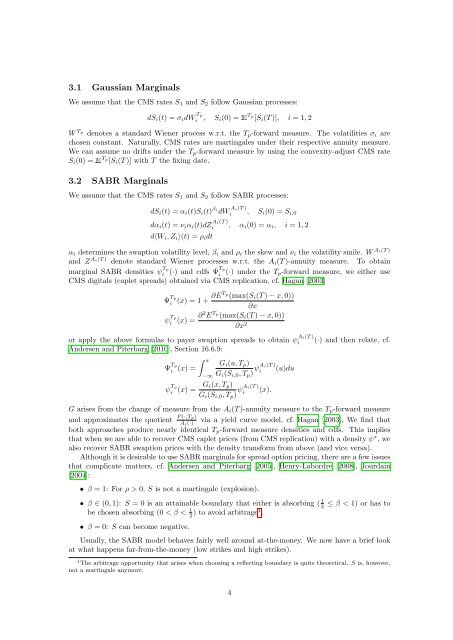
3.1 Gaussian Marginals
We assume that the CMS rates S1 and S2 follow Gaussian processes:
dSi(t) = σidW Tp
i , Si(0) = Tp [Si(T )], i = 1, 2
W Tp denotes a standard Wiener process w.r.t. the Tp-forward measure. The volatilities σi are
chosen constant. Naturally, CMS rates are martingales under their respective annuity measure.
We can assume no drifts under the Tp-forward measure by using the convexity-adjust CMS rate
Si(0) = Tp [Si(T )] with T the fixing date.
3.2 SABR Marginals
We assume that the CMS rates S1 and S2 follow SABR processes:
dSi(t) = αi(t)Si(t) βi Ai(T )
dWi , Si(0) = Si,0
Ai(T )
dαi(t) = νiαi(t)dZi ,
d〈Wi, Zi〉(t) = ρidt
αi(0) = αi, i = 1, 2
Ai(T )
αi determines the swaption volatility level, βi and ρi the skew and νi the volatility smile. W
and ZAi(T ) denote standard Wiener processes w.r.t. the Ai(T )-annuity measure. To obtain
marginal SABR densities ψ Tp
i
(·) and cdfs ΨTp
i (·) under the Tp-forward measure, we either use
CMS digitals (caplet spreads) obtained via CMS replication, cf. Hagan [2003]
Ψ Tp
i (x) = 1 + ∂ETp (max(Si(T ) − x, 0))
∂x
ψ Tp
i (x) = ∂2E Tp (max(Si(T ) − x, 0))
∂x2 or apply the above formulas to payer swaption spreads to obtain ψ
Andersen and Piterbarg [2010], Section 16.6.9:
Ψ Tp
i (x) =
x
−∞
Gi(u, Tp)
Gi(Si,0, Tp)
ψ Tp
i (x) = Gi(x, Tp)
Gi(Si,0, Tp)
)
ψAi(T i (u)du
)
ψAi(T i (x).
Ai(T )
i
(·) and then relate, cf.
G arises from the change of measure from the Ai(T )-annuity measure to the Tp-forward measure
P (·,Tp)
and approximates the quotient Ai(·) via a yield curve model, cf. Hagan [2003], We find that
both approaches produce nearly identical Tp-forward measure densities and cdfs. This implies
that when we are able to recover CMS caplet prices (from CMS replication) with a density ψ∗ , we
also recover SABR swaption prices with the density transform from above (and vice versa).
Although it is desirable to use SABR marginals for spread option pricing, there are a few issues
that complicate matters, cf. Andersen and Piterbarg [2005], Henry-Labordre [2008], Jourdain
[2004]:
• β = 1: For ρ > 0, S is not a martingale (explosion).
• β ∈ (0, 1): S = 0 is an attainable boundary that either is absorbing ( 1 ≤ β < 1) or has to
be chosen absorbing (0 < β < 1
2 ) to avoid arbitrage1 .
• β = 0: S can become negative.
Usually, the SABR model behaves fairly well around at-the-money. We now have a brief look
at what happens far-from-the-money (low strikes and high strikes).
1 The arbitrage opportunity that arises when choosing a reflecting boundary is quite theoretical. S is, however,
not a martingale anymore.
4
2