unit 1 metal cutting and chip formation - IGNOU
unit 1 metal cutting and chip formation - IGNOU
unit 1 metal cutting and chip formation - IGNOU

You also want an ePaper? Increase the reach of your titles
YUMPU automatically turns print PDFs into web optimized ePapers that Google loves.
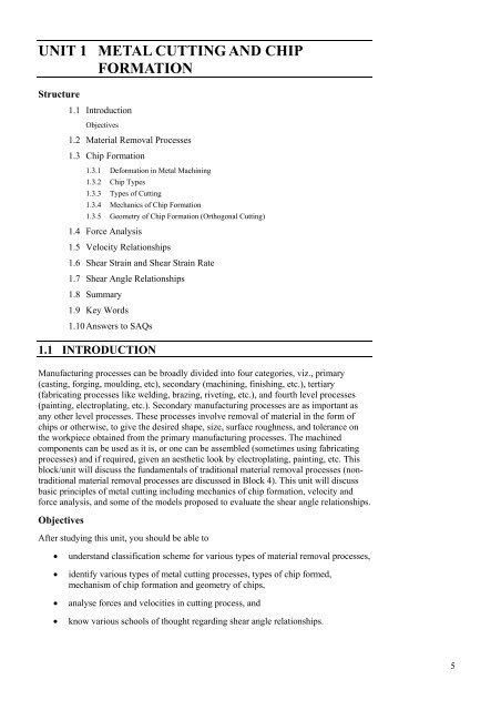
UNIT 1 METAL CUTTING AND CHIP<br />
FORMATION<br />
Structure<br />
1.1 Introduction<br />
Objectives<br />
1.2 Material Removal Processes<br />
1.3 Chip Formation<br />
1.3.1 De<strong>formation</strong> in Metal Machining<br />
1.3.2 Chip Types<br />
1.3.3 Types of Cutting<br />
1.3.4 Mechanics of Chip Formation<br />
1.3.5 Geometry of Chip Formation (Orthogonal Cutting)<br />
1.4 Force Analysis<br />
1.5 Velocity Relationships<br />
1.6 Shear Strain <strong>and</strong> Shear Strain Rate<br />
1.7 Shear Angle Relationships<br />
1.8 Summary<br />
1.9 Key Words<br />
1.10 Answers to SAQs<br />
1.1 INTRODUCTION<br />
Manufacturing processes can be broadly divided into four categories, viz., primary<br />
(casting, forging, moulding, etc), secondary (machining, finishing, etc.), tertiary<br />
(fabricating processes like welding, brazing, riveting, etc.), <strong>and</strong> fourth level processes<br />
(painting, electroplating, etc.). Secondary manufacturing processes are as important as<br />
any other level processes. These processes involve removal of material in the form of<br />
<strong>chip</strong>s or otherwise, to give the desired shape, size, surface roughness, <strong>and</strong> tolerance on<br />
the workpiece obtained from the primary manufacturing processes. The machined<br />
components can be used as it is, or one can be assembled (sometimes using fabricating<br />
processes) <strong>and</strong> if required, given an aesthetic look by electroplating, painting, etc. This<br />
block/<strong>unit</strong> will discuss the fundamentals of traditional material removal processes (nontraditional<br />
material removal processes are discussed in Block 4). This <strong>unit</strong> will discuss<br />
basic principles of <strong>metal</strong> <strong>cutting</strong> including mechanics of <strong>chip</strong> <strong>formation</strong>, velocity <strong>and</strong><br />
force analysis, <strong>and</strong> some of the models proposed to evaluate the shear angle relationships.<br />
Objectives<br />
After studying this <strong>unit</strong>, you should be able to<br />
• underst<strong>and</strong> classification scheme for various types of material removal processes,<br />
• identify various types of <strong>metal</strong> <strong>cutting</strong> processes, types of <strong>chip</strong> formed,<br />
mechanism of <strong>chip</strong> <strong>formation</strong> <strong>and</strong> geometry of <strong>chip</strong>s,<br />
• analyse forces <strong>and</strong> velocities in <strong>cutting</strong> process, <strong>and</strong><br />
• know various schools of thought regarding shear angle relationships.<br />
Metal Cutting <strong>and</strong><br />
Chip Formation<br />
5
Theory of Metal Cutting<br />
6<br />
1.2 MATERIAL REMOVAL PROCESSES<br />
Material removal processes can broadly be divided into two categories : traditional <strong>and</strong><br />
advanced (non-traditional). Each of these categories can be further sub-divided into bulk<br />
removal processes (or <strong>cutting</strong>) <strong>and</strong> finishing processes. The classification of various types<br />
of material removal processes is shown in Figure 1.1(a). This <strong>unit</strong> will discuss only the<br />
basics of traditional <strong>cutting</strong> processes.<br />
Traditional Cutting<br />
Traditional <strong>cutting</strong> processes can be classified as those which produce parts having<br />
surfaces of revolution <strong>and</strong> those which produce prismatic shapes. Another scheme<br />
for the classification of <strong>metal</strong> <strong>cutting</strong> processes is provided in<br />
Figure 1.1(a). This classification is based on the type of motion imparted to the<br />
work <strong>and</strong> tool. Cutting tools used for material removal are classified in two<br />
categories : single point <strong>cutting</strong> tool <strong>and</strong> multi-point <strong>cutting</strong> tool (<strong>cutting</strong> tools<br />
having more than one <strong>cutting</strong> edge). The following section discusses how material<br />
removal takes place by using a single point <strong>cutting</strong> tool. Similar principles are<br />
applicable to the multiple point <strong>cutting</strong> tools as well.<br />
Figure 1.1(a) : Classification of Material Removal Processes<br />
The process of <strong>metal</strong> <strong>cutting</strong> is effected by providing relative motion between the<br />
workpiece <strong>and</strong> the hard edge of <strong>cutting</strong> tool. Such relative motion is produced by a<br />
combination of rotary <strong>and</strong> translating movements either of the workpiece or of the<br />
<strong>cutting</strong> tool or both. Depending on the nature of the relative motion, <strong>metal</strong> <strong>cutting</strong><br />
process is called either turning or planning or boring, etc.<br />
For different types of operations, one needs to have different types of machine<br />
tools. For example, lathe for turning, planer for planning, grinder for grinding, etc.<br />
Some of these machines (say, lathe, boring m/c, <strong>and</strong> drill) generate surfaces of<br />
revolution whereas others (planer, milling m/c, <strong>and</strong> shaper) make prismatic (or flat<br />
surfaces) parts. With the help of different types of tools, a lathe can perform<br />
various kinds of operations (Figure 1.1(b)).<br />
Conventionally, the translatory displacement of the <strong>cutting</strong> edge of the tool along<br />
the work surface during a given period of time is called ‘feed’( f ), while the<br />
relative rate of traverse of work surface past the <strong>cutting</strong> edge is designated as the<br />
‘<strong>cutting</strong> velocity’ or simply ‘speed’ (Vc).<br />
In case of single point turning, Vc is the peripheral velocity of the rotating<br />
workpiece in meters per minute. In case of slab milling, it is the peripheral velocity<br />
of the milling cutter in meters/minute.
Figure 1.1(b) : Various Operations that can be Performed on a Lathe [Kalpakjian, 1989]<br />
Table 1.1<br />
Operation Motion of Job Motion of Cutting Tool Figure of Operation<br />
Turning on a<br />
lathe<br />
Boring on a<br />
lathe<br />
Drilling on a<br />
drill machine<br />
Rotary motion of the<br />
work<br />
Axial movement of the tool<br />
Work rotation Axial tool movement<br />
Fixed Rotations as well as<br />
translatory feed<br />
Planning Translatory Intermittent Translation<br />
Milling Translatory Rotation<br />
Grinding Rotary/Translatory Rotary<br />
Metal Cutting <strong>and</strong><br />
Chip Formation<br />
7
Theory of Metal Cutting<br />
8<br />
1.3 CHIP FORMATION<br />
1.3.1 De<strong>formation</strong> in Metal Machining<br />
Figure 1.2 shows a schematic diagram of material de<strong>formation</strong> during <strong>cutting</strong>, <strong>and</strong><br />
subsequently removal of the deformed material from the workpiece by a single point<br />
<strong>cutting</strong> tool. Because of the relative motion between the tool <strong>and</strong> the workpiece, material<br />
ahead of the tool face (rake face) is compressed (elastically <strong>and</strong> then plastically). Further,<br />
movement of the tool into the workpiece deforms the work material plastically <strong>and</strong><br />
finally separates the deformed material from the workpiece. This separated material<br />
flows on the rake face of the tool called as <strong>chip</strong>. The <strong>chip</strong> near the end of the rake face is<br />
lifted away from the tool, <strong>and</strong> the resultant curvature of the <strong>chip</strong> is called <strong>chip</strong> curl.<br />
Figure 1.2 : Schematic Diagram of Chip De<strong>formation</strong><br />
The study of the mechanism of <strong>chip</strong> <strong>formation</strong> involves de<strong>formation</strong> process of the <strong>chip</strong><br />
ahead of the <strong>cutting</strong> tool. Theoretical study of the material de<strong>formation</strong> in <strong>metal</strong> <strong>cutting</strong> is<br />
difficult <strong>and</strong> therefore experimental techniques have been resorted to for analyzing the<br />
process of de<strong>formation</strong> in <strong>chip</strong>s. The methods commonly employed for this purpose are :<br />
(i) Use of movie camera for taking pictures of <strong>chip</strong>.<br />
(ii) Observing grid de<strong>formation</strong> during <strong>cutting</strong>.<br />
(iii) Examination of frozen <strong>chip</strong> samples obtained by the use of quick-stop<br />
device.<br />
Experimental study of <strong>chip</strong> de<strong>formation</strong> process has revealed that :<br />
(i) During machining of ductile materials, a plastic de<strong>formation</strong> zone is formed<br />
in front of the <strong>cutting</strong> edge (Figure 1.2).<br />
(ii) The distinctive zone of separation between the <strong>chip</strong> <strong>and</strong> workpiece where<br />
de<strong>formation</strong> gradually increases towards the <strong>cutting</strong> edge is called the<br />
primary de<strong>formation</strong>/shear zone. In shear zone extensive de<strong>formation</strong><br />
occurs. The width of shear zone is very small.<br />
(iii) The plastic de<strong>formation</strong> involved in the <strong>formation</strong> of <strong>chip</strong>s affects the<br />
hardness of material (strain hardening). Strain hardening increases when a<br />
layer undergoes de<strong>formation</strong> in the shear zone.<br />
1.3.2 Chip Types<br />
The type of <strong>chip</strong> obtained from a machining process is characterized by a number of<br />
parameters e.g., the type of tool-work engagement, work material properties <strong>and</strong> the<br />
<strong>cutting</strong> conditions.<br />
Ernst has classified the <strong>chip</strong>s obtained in machining processes into three categories :<br />
Type 1 : Discontinuous <strong>chip</strong>,
Type 2 : Continuous <strong>chip</strong>, <strong>and</strong><br />
Type 3 : Continuous with built-up edge.<br />
When ductile materials at high <strong>cutting</strong> speed are cut by a single point <strong>cutting</strong> tool, ribbon<br />
like continuous <strong>chip</strong> (Figure 1.3(a) <strong>and</strong> 1.3 (b)) is obtained. The conditions that promote<br />
<strong>formation</strong> of continuous <strong>chip</strong>s in <strong>metal</strong> <strong>cutting</strong> are sharp <strong>cutting</strong> edge, low feed rate (or<br />
small <strong>chip</strong> thickness), large rake angle, ductile work material, high <strong>cutting</strong> speed, <strong>and</strong> low<br />
friction at <strong>chip</strong>-tool interface. As shown in Figure 1.2, major de<strong>formation</strong> takes place in<br />
primary shear de<strong>formation</strong> zone (PSDZ) resulting in the <strong>formation</strong> of <strong>chip</strong>. Due to ductile<br />
nature of work material <strong>and</strong> reasonably high temperature in the PSDZ, the deforming<br />
material flows on the rake face of the tool as continuous mass rather than the one<br />
fractured/ruptured at small distances at the underneath of the <strong>chip</strong> as in discontinuous<br />
<strong>chip</strong>.<br />
Continuous <strong>chip</strong> results in good surface finish, high tool-life, <strong>and</strong> low power<br />
consumption. But disposal of large coiled <strong>chip</strong>s is a serious problem, for many industries<br />
where tons of <strong>chip</strong>s are produced every week. To get rid of this problem various types of<br />
<strong>chip</strong> breakers are used which are in the form of step or groove on the rake face of the<br />
tool (Figure 1.4). The <strong>chip</strong> strikes with this step/groove <strong>and</strong> gets broken in the form of<br />
small segments. Disposal of such small <strong>chip</strong>s is not a problem.<br />
If the friction between tool <strong>and</strong> <strong>chip</strong> while machining ductile materials is high, some part<br />
of the <strong>chip</strong> gets welded to the rake face of the tool near its <strong>cutting</strong> edge. The welded<br />
material is extremely hard <strong>and</strong> its size keeps on increasing with time. Because of the<br />
hardness of the adhered materials onto the <strong>cutting</strong> edge, it participates in <strong>cutting</strong> to a<br />
certain extent. That is why it is named as built up edge (Figure 1.5). As the size of the<br />
BUE grows larger, it becomes unstable <strong>and</strong> it breaks. Some part from the broken BUE is<br />
carried away by the <strong>chip</strong> as well as on the machined surface (Figure 1.3).<br />
Figure 1.3 : Different Kinds of Chips : (a) Continuous; (b) Photograph of Continuous Chip;<br />
(c) Continuous Chip with Built Up Edge; <strong>and</strong> (d) Discontinuous Chip<br />
The <strong>chip</strong> with the adhered parts of the BUE is known as continuous <strong>chip</strong> with BUE. The<br />
adhered parts of the BUE on the machined surface make the machined surface rough, but<br />
the BUE protects the actual <strong>cutting</strong> edge of the tool from wear. Thus, <strong>cutting</strong> with BUE<br />
enhances the tool life (or tool cuts longer before regrind).<br />
Metal Cutting <strong>and</strong><br />
Chip Formation<br />
9
Theory of Metal Cutting<br />
10<br />
Figure 1.4 : Different Types of Chip Breakers<br />
Figure 1.5 : Development of Built Up Edge [Rao, 2000]<br />
Discontinuous or segmented <strong>chip</strong>s are produced while machining brittle materials or<br />
ductile materials at low speeds <strong>and</strong> high friction conditions. The basic difference between<br />
the mechanism of <strong>formation</strong> of discontinuous <strong>chip</strong> <strong>and</strong> continuous <strong>chip</strong> is that, instead of<br />
continuous shearing of the material ahead of the <strong>cutting</strong> tool, rupture occurs<br />
intermittently producing segments of <strong>chip</strong> (Figures 1.3 <strong>and</strong> 1.6). These <strong>chip</strong>s are smaller<br />
in length hence easy to dispose off, <strong>and</strong> give good surface finish on the workpiece.<br />
Discontinuous <strong>chip</strong>s are formed when <strong>cutting</strong> brittle materials, or <strong>cutting</strong> ductile<br />
materials at low speed, or <strong>cutting</strong> with tools of small rake angle.<br />
1.3.3 Types of Cutting<br />
(a) Tear Type (b) Shear Type<br />
Figure 1.6 : Hypothesized Discontinuous Chip Formation [Rao, 2000]<br />
Principally, there are two types of <strong>cutting</strong> :<br />
(i) Orthogonal <strong>cutting</strong>, <strong>and</strong><br />
(ii) Oblique <strong>cutting</strong>.<br />
Orthogonal Cutting<br />
Orthogonal <strong>cutting</strong> operation is “the simplest type of <strong>cutting</strong> operation, in which<br />
the <strong>cutting</strong> edge is straight, parallel to the original plane surface of the workpiece<br />
<strong>and</strong> perpendicular to the direction of <strong>cutting</strong>, <strong>and</strong> in which the length of the <strong>cutting</strong><br />
edge is greater than the width of the <strong>chip</strong> removed (Figures 1.7(a) <strong>and</strong> (b))”. This<br />
orthogonal <strong>cutting</strong> is also known as Two Dimensional (2-D) Cutting. A few of the<br />
<strong>cutting</strong> tools perform orthogonally, such as lathe cut-off tools (Figure 1.7(a)),<br />
straight (not helical) milling cutters, broaches, etc.<br />
In actual machining, majority of the <strong>cutting</strong> operations (turning, milling, etc.) are<br />
three dimensional (3-D) in nature <strong>and</strong> are called as oblique <strong>cutting</strong>. In oblique<br />
<strong>cutting</strong>, the <strong>cutting</strong> edge of the tool is inclined to the line normal to the <strong>cutting</strong><br />
direction, <strong>and</strong> this angle is known as angle of obliquity. This is also called the<br />
inclination angle, i (Figure 1.7(c)). Oblique <strong>cutting</strong> can be defined as “the <strong>cutting</strong>
operation in which the <strong>cutting</strong> edge is straight <strong>and</strong> parallel to the original surface of<br />
the workpiece, but is not perpendicular to the <strong>cutting</strong> direction, being inclined to<br />
it”. An angle of interest in this case is the <strong>chip</strong> flow angle, ηc which is defined as<br />
the angle measured in the plane of <strong>cutting</strong> face between the <strong>chip</strong> flow direction <strong>and</strong><br />
the normal to the <strong>cutting</strong> edge (Figure 1.7(c)). Both ‘i’ <strong>and</strong> ηc are zero in case of<br />
orthogonal <strong>cutting</strong>. The certain practical limitations to orthogonal <strong>cutting</strong> are<br />
mitigated by three dimensional tooling.<br />
Figure 1.7 : (a); (b) Orthogonal Cutting System; <strong>and</strong> (c) Oblique Cutting System<br />
Generally for the mathematical analysis of the mechanics of <strong>metal</strong> <strong>cutting</strong>, orthogonal<br />
<strong>cutting</strong> is considered because it is simpler than the oblique <strong>cutting</strong>. The results so<br />
obtained can be used for oblique <strong>cutting</strong> operations.<br />
1.3.4 Mechanics of Chip Formation<br />
Plastic de<strong>formation</strong> is the main factor that governs <strong>formation</strong> of <strong>chip</strong>s. Initially,<br />
researchers (Merchant <strong>and</strong> others) proposed that de<strong>formation</strong> of the material takes place<br />
along a plane (called shear plane) just ahead of the <strong>cutting</strong> tool <strong>and</strong> runs up to free<br />
surface of the workpiece (Figure 1.8(a)). Once the deforming material crosses the shear<br />
plane, it slides along the rake face of the tool due to the velocity of <strong>cutting</strong> tool (relative<br />
motion between the tool <strong>and</strong> workpiece). This hypothesis of a shear plane is useful from<br />
the analysis of <strong>metal</strong> <strong>cutting</strong> point of view but has theoretical drawbacks. Here, the<br />
transition from the un-deformed to the deformed material takes place along a shear plane<br />
by changing <strong>cutting</strong> velocity from Vc (velocity of tool with respect to workpiece) to Vf<br />
(<strong>chip</strong> velocity relative to the tool). For this change to take place, the acceleration across<br />
the plane (plane thickness equal to zero) has to be infinite. This also applies to the<br />
stress-gradient across the shear plane. Due to the above anomaly, researchers (Oxley <strong>and</strong><br />
others) experimentally studied the de<strong>formation</strong> zone by freezing the <strong>cutting</strong> process with<br />
the help of a quick stop device. When they studied the deformed zone under a<br />
microscope, they found that the de<strong>formation</strong> takes place within a finite zone (thin or thick<br />
depending upon various governing parameters). This is called as primary shear<br />
de<strong>formation</strong> zone (PSDZ) (Figures 1.8 (b) <strong>and</strong> (c)). They also found that under certain<br />
machining conditions, de<strong>formation</strong> also takes place at the tool-<strong>chip</strong> interface<br />
Metal Cutting <strong>and</strong><br />
Chip Formation<br />
11
Theory of Metal Cutting<br />
12<br />
(Figures 1.8 (b) <strong>and</strong> (c)). This de<strong>formation</strong> is known as secondary shear de<strong>formation</strong><br />
zone (SSDZ).<br />
Figure 1.8 : (a) Shear Plane; (b) Primary <strong>and</strong> Secondary Shear De<strong>formation</strong> Zone in Chip Formation;<br />
<strong>and</strong> (c) Frozen Chip Obtained by a Quick Stop Device<br />
1.3.5 Geometry of Chip Formation (Orthogonal Cutting)<br />
Figure 1.9 shows a simple geometry of <strong>chip</strong> <strong>formation</strong> in case of continuous <strong>chip</strong><br />
(type 2). The uncut <strong>chip</strong> thickness tu (equal to feed in turning) is deformed to give <strong>chip</strong><br />
thickness tc which experiences two velocities Vf (<strong>chip</strong> sliding velocity) <strong>and</strong> Vs (shear<br />
velocity) along the tool face <strong>and</strong> shear plane, respectively. From this geometry, it is<br />
possible to calculate the shear angle (φ) in terms of measurable or known quantities tu, tc<br />
<strong>and</strong> α.<br />
Figure 1.9 : Geometry of Continuous Chip Formation<br />
From right angle triangles, ABC <strong>and</strong> ABD (BD is perpendicular to AD drawn from B),<br />
AB = tu / sin φ<br />
Also, AB = tc / sin (90 − (φ −α)) = tc / cos (φ −α)<br />
∴<br />
t<br />
t<br />
u<br />
c<br />
sin φ<br />
=<br />
cos ( φ − α)
tu<br />
is called <strong>chip</strong> thickness ratio or <strong>chip</strong> thickness coefficient (rc) which can be written<br />
tc<br />
as<br />
1 cosφ<br />
cosα<br />
+ sin φsin<br />
α<br />
=<br />
sin φ<br />
rc<br />
or, 1 = rc cot φcos<br />
α + rc<br />
sin α<br />
or,<br />
∴<br />
rc<br />
cos α = ( 1−<br />
rc<br />
sin α)<br />
tan φ<br />
⎛ r cos<br />
tan c α ⎞<br />
φ=⎜ ⎟ . . . (1.1)<br />
⎝1− r c sin α⎠<br />
To determine the shear plane angle (φ) for a given <strong>cutting</strong> condition the <strong>chip</strong> thickness<br />
⎛ t ⎞<br />
ratio<br />
⎜ u r c =<br />
⎟ , should be known. But to determine tc with a micrometer is somewhat<br />
⎝ tc<br />
⎠<br />
inaccurate. Hence, an indirect approach to this problem is to assume that the density of<br />
<strong>metal</strong> during the <strong>cutting</strong> process does not change. Hence, the volume of uncut <strong>chip</strong> is<br />
equal to the volume of <strong>metal</strong> removed (or deformed <strong>chip</strong>). Since the width of <strong>chip</strong> (b) is<br />
equal to the width of <strong>metal</strong> being cut (in orthogonal <strong>cutting</strong>), therefore :<br />
∴ Lctc= Lutu or,<br />
bLc tc<br />
= Lutub<br />
(volume constancy condition)<br />
t u L<br />
=<br />
c<br />
tc<br />
Lu<br />
tu L<br />
∴ rc<br />
= =<br />
t L<br />
c . . . (1.2)<br />
c u<br />
where, Lc is length of <strong>chip</strong>, <strong>and</strong> Lu is corresponding length of material removed from the<br />
workpiece (or uncut <strong>chip</strong> length). Lc can be easily measured, <strong>and</strong> it (Lc / Lu) will give<br />
more accurate results than (tu / tc) because of the difficulties <strong>and</strong> inaccuracies involved in<br />
the measurement of thickness of the deformed <strong>chip</strong> (tc).<br />
1.4 FORCE ANALYSIS<br />
Let us analyse the forces acting on the <strong>chip</strong> in orthogonal <strong>cutting</strong>. These are shown in<br />
Figure 1.10 (a) <strong>and</strong> are as follows : Force, Fs, is the resistance to shear of the <strong>metal</strong> in<br />
forming the <strong>chip</strong>. Fs acts along the shear plane. Force, Fn, is normal to the shear plane<br />
<strong>and</strong> is a backup force on the <strong>chip</strong> provided by the workpiece. Force N acting on the <strong>chip</strong><br />
is normal to the <strong>cutting</strong> face of the tool <strong>and</strong> is provided by the tool. Force F is frictional<br />
resistance offered by the tool to the <strong>chip</strong> flow. The latter force acts downwards against<br />
the motion of the <strong>chip</strong> as it slides upwards along the tool face.<br />
Figure 1.10 (b) shows the free body diagram of the forces acting on the <strong>chip</strong>. Forces Fs<br />
<strong>and</strong> Fn are represented by the resultant R, <strong>and</strong> F <strong>and</strong> N are replaced by the resultant R'.<br />
This means that only two combined forces are acting on the <strong>chip</strong>, i.e., R <strong>and</strong> R'. There are<br />
external couples on the <strong>chip</strong> which curl it, <strong>and</strong> they may be negated in this approximate<br />
analysis. If equilibrium is to exist when a body is acted upon by two forces, they must be<br />
equal in magnitude, <strong>and</strong> be collinear. Hence, R <strong>and</strong> R' are equal in magnitude, opposite in<br />
direction <strong>and</strong> collinear (Figure 1.10).<br />
Metal Cutting <strong>and</strong><br />
Chip Formation<br />
13
Theory of Metal Cutting<br />
14<br />
Figure 1.10 : (a) Force Components Acting on a Chip; <strong>and</strong> (b) Free Body Diagram of a Chip<br />
Figure 1.11 shows a composite diagram in which the two force triangles of<br />
Figure 1.10, have been superimposed by placing the two equal forces R <strong>and</strong> R ' together.<br />
Since the angle between Fs <strong>and</strong> Fn is a right angle, the intersection of these forces lies on<br />
the circle with diameter R as shown. Also, F <strong>and</strong> N may be replaced by R to form the<br />
circle diagram (Figure 1.11).<br />
Figure 1.11 : Force Circle Diagram<br />
The horizontal <strong>cutting</strong> force Fc <strong>and</strong> vertical force Ft can be measured in a machining<br />
operation by the use of a force dynamometer. The electric strain gauge type of transducer<br />
is used in the dynamometer. After Fc <strong>and</strong> Ft are determined, they can be laid off as in<br />
Figure 1.11 <strong>and</strong> their resultant is the diameter of the circle. The rake angle α can be laid<br />
off, <strong>and</strong> the forces F <strong>and</strong> N can then be determined. The shear plane angle φ can be<br />
measured approximately from a photomicrograph or by measuring tc <strong>and</strong> tu, or length of<br />
<strong>chip</strong> <strong>and</strong> corresponding length of unmachined <strong>chip</strong> (discussed elsewhere).<br />
From Figure 1.11, the following vector Eqs. can be written<br />
ρ ρ ρ<br />
R'<br />
= F + N<br />
ρ ρ ρ ρ ρ ρ<br />
R = Fs<br />
+ Fn<br />
= Fc<br />
+ Ft<br />
= R'<br />
Merchant represented various forces in a force circle diagram in which tool <strong>and</strong> reaction<br />
forces have been assumed to be acting as concentrated at the tool point instead of their<br />
actual points of application along the tool face <strong>and</strong> the shear plane. The circle has the<br />
diameter equal to R (or R') passing through tool point.<br />
After Fc, Ft, α <strong>and</strong> φ are known, all the component forces on the <strong>chip</strong> may be determined<br />
from the geometry. For instance, the average stress on the shear plane can be determined<br />
by using force Fs <strong>and</strong> the area of the shear plane. Another useful quantity is the<br />
coefficient of friction (μ) between the tool <strong>and</strong> <strong>chip</strong>. Using force circle diagram, it can be<br />
shown that
F = Ft<br />
cosα + Fc<br />
sin α<br />
. . . (1.3) Metal Cutting <strong>and</strong><br />
Chip Formation<br />
<strong>and</strong>, N = Fc<br />
cos α − Ft<br />
sin α<br />
. . . (1.4)<br />
Then, the coefficient of friction (μ) is calculated as<br />
μ =<br />
where, β is the friction angle.<br />
or,<br />
We can also write :<br />
μ =<br />
β =<br />
β =<br />
From Figure 1.11, we get :<br />
Also, from Figure 1.11,<br />
or,<br />
F<br />
∴<br />
F<br />
tanβ<br />
=<br />
F<br />
N<br />
Ft<br />
+ Fc<br />
tan α<br />
Fc<br />
− Ft<br />
tan α<br />
tan<br />
−1<br />
( μ)<br />
F α + α<br />
=<br />
t cos Fc<br />
sin<br />
Fc<br />
cosα<br />
− Ft<br />
sin α<br />
. . . (1.5)<br />
. . . (1.6)<br />
− ⎧ + tan α⎫<br />
tan<br />
1 F t F<br />
. . . (1.7)<br />
c<br />
⎨<br />
⎬<br />
⎩ Fc<br />
− Ft<br />
tan α ⎭<br />
F s = Fc<br />
cos φ − Ft<br />
sin φ<br />
. . . (1.8)<br />
F n = Ft<br />
cos φ + Fc<br />
sin φ<br />
F n = Fs<br />
tan( φ + β − α)<br />
. . . (1.9)<br />
F<br />
c<br />
s<br />
c<br />
s<br />
= R<br />
cos(β<br />
− α)<br />
F = R cos(<br />
φ+<br />
β − α)<br />
F<br />
Shear plane area is equal to :<br />
c<br />
cos(<br />
β −α)<br />
=<br />
cos(<br />
φ + β − α)<br />
cos(<br />
β−<br />
α)<br />
= Fs<br />
cos(<br />
φ + β − α)<br />
. . . (1.9(a))<br />
t b<br />
A =<br />
u<br />
s . . . (1.10)<br />
sin φ<br />
If τ be the shear strength of the work material, then,<br />
Substituting in Eq.(1.9 (a)), we get<br />
hence,<br />
t b<br />
F =<br />
u<br />
s τ<br />
. . . (1.11)<br />
sin φ<br />
⎛ t b<br />
F<br />
u τ ⎞ cos( β − α)<br />
c = ⎜ ⎟<br />
. . . (1.12)<br />
⎝ sin φ ⎠ cos( φ + β − α)<br />
t bτ<br />
R =<br />
u<br />
. . . (1.12(a))<br />
sin φcos(<br />
φ + β − α)<br />
15
Theory of Metal Cutting<br />
16<br />
From Figure 1.11,<br />
Ft<br />
= Rsin(<br />
β − α)<br />
t τ<br />
= ub<br />
(From Eq. 1.12(a)) . . . (1.13)<br />
sin ( β − α)<br />
sin φcos<br />
( φ + β − α)<br />
From Eqs. (1.12) <strong>and</strong> (1.13), we can write :<br />
Ft<br />
= tan ( β − α)<br />
. . . (1.14)<br />
Fc<br />
From the above analysis, unknown forces in the force circle diagram <strong>and</strong> the value of<br />
coefficient of friction can be calculated provided Fc, Ft, α, tu <strong>and</strong> tc are known measured.<br />
During machining operations, <strong>chip</strong>s are formed as a result of plastic de<strong>formation</strong>. Hence,<br />
<strong>chip</strong>s experience stresses <strong>and</strong> strains. At shear plane, two normal forces simultaneously<br />
act, i.e., Fs <strong>and</strong> Fn. Shear stress (τ) can be found as<br />
F ( cosφ<br />
− sin φ)<br />
Mean shear stress ( τ) =<br />
s F<br />
=<br />
c Ft<br />
sin φ<br />
As<br />
btu<br />
Mean Normal stress (σ)<br />
where, As = Shear plane area = b tu<br />
/ sin φ .<br />
1.5 VELOCITY RELATIONSHIPS<br />
. . . (1.15)<br />
Fn sin φ<br />
= = ( Ft<br />
cosφ<br />
+ Fc<br />
sin φ)<br />
. . . (1.16)<br />
As<br />
btu<br />
Since the <strong>chip</strong> is thicker than the uncut <strong>chip</strong>, the velocity of the <strong>chip</strong> as it moves along the<br />
tool face must be less than the <strong>cutting</strong> speed (assuming volume constancy during <strong>cutting</strong>,<br />
<strong>and</strong> width of cut before machining <strong>and</strong> after machining remains same). Different<br />
velocities during <strong>cutting</strong> can be estimated as follows :<br />
Assume that the <strong>cutting</strong> velocity of the tool relative to the workpiece is Vc which is<br />
known before h<strong>and</strong>. The <strong>chip</strong> slides along the <strong>cutting</strong> (rake) face of the tool with a<br />
velocity relative to the tool equal to Vf (<strong>chip</strong> flow velocity). The newly cut <strong>chip</strong> elements<br />
move relative to the workpiece along the shear plane with a velocity equal to Vs (shear<br />
velocity). From the principle of kinematics that the relative velocity of two bodies (here<br />
tool <strong>and</strong> <strong>chip</strong>) is equal to the vector difference between their velocities relative to the<br />
reference body (the workpiece). Employing this principle, Figure 1.12 has been drawn.<br />
Using sine rule, from Δ ABC, we get :<br />
or,<br />
V V<br />
c f Vs<br />
= =<br />
. . . (1.17)<br />
sin ( 90 − ( φ − α))<br />
sin φ sin ( 90 − α)<br />
V V<br />
c<br />
f Vs<br />
= =<br />
cos( φ − α)<br />
sin φ cosα<br />
The <strong>chip</strong> flow velocity along the tool rake face is given by<br />
Vc<br />
sin φ<br />
=<br />
cos(<br />
φ − α)<br />
V f<br />
=Vc . rc . . . (1.18)<br />
whereas the shear velocity Vs is obtained as :
V cosα<br />
V =<br />
c<br />
s<br />
. . . (1.19)<br />
cos(<br />
φ − α)<br />
Figure 1.12 : Velocity Relationship<br />
1.6 SHEAR STRAIN AND SHEAR STRAIN RATE<br />
Since most practical <strong>cutting</strong> processes are geometrically complex, let us first study the<br />
orthogonal machining <strong>and</strong> extend the theory of orthogonal <strong>cutting</strong> to more complicated<br />
<strong>cutting</strong> process involving oblique <strong>cutting</strong>. Due to simplicity <strong>and</strong> fairly wide applications,<br />
the continuous <strong>chip</strong> without BUE has been most extensively studied. There are<br />
conflicting evidences about the nature of the de<strong>formation</strong> zone in <strong>metal</strong> <strong>cutting</strong>. This has<br />
led to two basic schools of thought in the approach to the analysis.<br />
Many workers, such as Piispanen, Merchant, Kobayashi <strong>and</strong> Thomson have favoured the<br />
thin plane model while Palmer <strong>and</strong> Oxley, <strong>and</strong> Okushima <strong>and</strong> Hitomi have based their<br />
analysis on thick de<strong>formation</strong> region (Figure1.8). Experimental evidences indicate that<br />
the thick zone model may describe the <strong>cutting</strong> process at low speeds, but at high speeds<br />
most evidences indicate that a thin shear plane is approached. Thin zone model is more<br />
useful in practical <strong>cutting</strong> <strong>and</strong> its analysis is simpler hence it has received more attention.<br />
Thin Zone Model<br />
Merchant developed an analysis based on the thin shear plane model. He made the<br />
following assumptions :<br />
• The tool tip is sharp <strong>and</strong> no rubbing or ploughing occurs between the tool<br />
<strong>and</strong> the workpiece.<br />
• The de<strong>formation</strong> is two dimensional, i.e., no side spread.<br />
• The stress on the shear plane is uniformly distributed.<br />
• The resultant force R on the <strong>chip</strong> applied at the shear plane is equal, opposite<br />
<strong>and</strong> collinear to the force R' applied to the <strong>chip</strong> at the tool-<strong>chip</strong> interface.<br />
Strain <strong>and</strong> strain rate are determined as follows :<br />
To derive an expression for shear strain, the de<strong>formation</strong> can be idealized as a<br />
process of block slip (or preferred slip planes), as shown in (Figure 1.13). Shear<br />
strain (γ) is defined as the de<strong>formation</strong> per <strong>unit</strong> length.<br />
Δs<br />
γ = =<br />
Δy<br />
AB<br />
CD<br />
=<br />
AD<br />
CD<br />
+<br />
DB<br />
CD<br />
= tan ( φ − α)<br />
+ cot φ<br />
. . . (1.20)<br />
sin ( φ − α)<br />
cosφ<br />
= +<br />
cos(<br />
φ − α)<br />
sin φ<br />
sin ( φ − α)<br />
sin φ + cosφ<br />
cos(<br />
φ − α)<br />
=<br />
sin φcos(<br />
φ − α)<br />
Metal Cutting <strong>and</strong><br />
Chip Formation<br />
17
Theory of Metal Cutting<br />
18<br />
or,<br />
cos(<br />
φ+<br />
α −φ)<br />
cosα<br />
=<br />
=<br />
sin φcos(<br />
φ − α)<br />
sin φcos(<br />
φ − α)<br />
cosα<br />
γ =<br />
. . . (1.21)<br />
sin φcos(<br />
φ − α)<br />
Figure 1.13 : Strain <strong>and</strong> Strain Rate in Orthogonal Cutting<br />
Strain may also be expressed in terms of the shear velocity (Vs) <strong>and</strong> the <strong>chip</strong> velocity (Vf)<br />
∴<br />
γ=<br />
V<br />
Vs<br />
(from Eq.(1.19))<br />
sin φ<br />
c<br />
Therefore, shear strain rate (γ&) in <strong>cutting</strong> is given by<br />
⎛ Δs<br />
⎞<br />
⎜ ⎟<br />
dγ<br />
⎝ Δy<br />
⎠ ⎛ Δs<br />
⎞ 1<br />
γ&<br />
= = = ⎜ ⎟<br />
dt Δt<br />
⎝ Δt<br />
⎠ Δy<br />
V V<br />
γ& s c cosα<br />
= =<br />
Δy<br />
cos(<br />
φ − α)<br />
Δy<br />
Δy is mean thickness of PSDZ .<br />
1.7 SHEAR ANGLE RELATIONSHIPS<br />
. . . (1.22)<br />
A number of attempts have been made to study the mechanics of <strong>cutting</strong> process. In<br />
designing a <strong>metal</strong> <strong>cutting</strong> operation, it would be helpful to predict the position of the<br />
shear plane (angle φ). Attempts have been made to derive a fundamental relationship of<br />
the shear plane angle φ in terms of rake angle (α) <strong>and</strong> friction angle (β). Several theories<br />
have been proposed to establish a relationship between φ, α <strong>and</strong> β. Some of the theories<br />
have been discussed below.<br />
Ernst-Merchant derived a relationship using the minimum energy criterion, that is, the<br />
shear plane is located where the least energy is required for shear. The derivation of<br />
Ernst-Merchant equation is based on the following assumptions :<br />
(i) <strong>cutting</strong> is orthogonal,<br />
(ii) the shear strength of the <strong>metal</strong> along the shear plane is independent of the<br />
magnitude of compressive (normal) stress acting on that plane,<br />
(iii) the <strong>chip</strong> is continuous type with no built up edge, <strong>and</strong><br />
(iv) the energy of separation of <strong>chip</strong> elements is neglected <strong>and</strong> the minimum<br />
energy criterion establishes the plane on which shearing de<strong>formation</strong> occurs.
As the <strong>cutting</strong> progresses in the beginning, the <strong>cutting</strong> force (Fc) increases gradually, the<br />
shear stress on various planes ahead of the tool also increases. However, the shear stress<br />
will not be same on all the planes ahead of the tool because the shearing components of<br />
the forces on the planes are not the same, nor is the extent of areas the same. On one of<br />
the planes, however, the shear stress will be greater than on any other plane, <strong>and</strong> as Fc is<br />
further increased, the shear stress will reach the yield strength in shear of the material<br />
being cut <strong>and</strong> plastic de<strong>formation</strong> will occur along that plane, thus forming the <strong>chip</strong>. The<br />
<strong>cutting</strong> force required to cause shear de<strong>formation</strong> along that plane will then be the lowest<br />
<strong>cutting</strong> force. Once the shear de<strong>formation</strong> begins along one plane, the <strong>cutting</strong> force<br />
cannot exceed that minimum value.<br />
To determine shear-plane angle φ, express the <strong>cutting</strong> force Fc in terms of φ, differentiate<br />
it with respect to φ, equate the derivative to zero, <strong>and</strong> solve it for the angle φ as follows :<br />
cos(<br />
β − α)<br />
Fc<br />
= Fs<br />
cos<br />
τ tub<br />
=<br />
cos(<br />
β − α)<br />
{ φ + ( β − α)<br />
} sin φ cos(<br />
φ + β − α)<br />
×<br />
(Eq.1.12)<br />
Here, except φ all other parameters can be taken as constant during machining (assuming<br />
that no strain hardening takes place). It would give the condition for the minimum energy<br />
if the derivative of Fc with respect to φ is equated to zero.<br />
Therefore,<br />
d Fc<br />
d φ<br />
= τ<br />
t<br />
u<br />
⎡cosφ<br />
cos(<br />
φ+<br />
β − α)<br />
−sin<br />
φ(<br />
φ+<br />
β − α)<br />
⎤<br />
b cos(<br />
β − α)<br />
⎢<br />
= 0<br />
2 2<br />
⎥<br />
⎢⎣<br />
sin φcos<br />
( φ+<br />
β − α)<br />
⎥⎦<br />
cosφ cos ( φ +β−α) −sin φsin ( φ+β−α ) = 0<br />
or, cos (2 φ +β−α ) = 0<br />
or, (2 φ+β−α ) =<br />
π<br />
2<br />
π 1<br />
Hence, φ = − ( β − α)<br />
. . . (1.23)<br />
4 2<br />
where, φ, β <strong>and</strong> α are shear angle, friction angle <strong>and</strong> rake angle, respectively.<br />
Eq. (1.23) indicates that the shear angle φ is a unique function of the tool rake angle <strong>and</strong><br />
the angle of friction in <strong>metal</strong> <strong>cutting</strong>.<br />
Merchant further introduced a modification to this theory <strong>and</strong> assumed that the shear<br />
strength of a polycrystalline <strong>metal</strong> is affected by temperature, rate of shear, shear strain<br />
(plastic) <strong>and</strong> the stress acting normal to the shear plane. While it is known that the normal<br />
compression stress on a plane does not affect the shear strength of a single crystal<br />
however, the shear strength of polycrystalline material is affected. The modified Eq. is<br />
1<br />
φ = − ( β−<br />
α)<br />
2 2<br />
C<br />
. . . (1.24)<br />
where, ‘C’ depends on the slope of the shear strength vs. compressive stress curve for the<br />
given material. 'C' is also known as machining constant.<br />
In 1949, another approach to the analytical solution of the shear plane angle was made by<br />
Lee <strong>and</strong> Shaffer. They assumed that the material being cut behaves as an ideal plastic<br />
which does not strain harden. It was assumed that the shear plane coincides with the<br />
direction of the maximum shear stress (Figure 1.14). Based on these assumptions, they<br />
applied slip line field theory <strong>and</strong> derived the relationship given by Eq. (1.25).<br />
π<br />
φ = + ( α − β)<br />
. . . (1.25)<br />
4<br />
As a modification, later on Lee <strong>and</strong> Shaffer considered the effect of a small built up edge<br />
or nose, <strong>and</strong> its effect on the stress field referred to above <strong>and</strong> arrived at an expression for<br />
Metal Cutting <strong>and</strong><br />
Chip Formation<br />
19
Theory of Metal Cutting<br />
20<br />
the shear angle (φ) which included an additional angle θ, which depends on the size of<br />
the built up edge,<br />
π<br />
φ = + ( α − β)<br />
+ θ<br />
4<br />
In 1952, Shaw, Cook <strong>and</strong> Finnie extended the Lee <strong>and</strong> Schaffer theory by further<br />
analytical <strong>and</strong> experimental investigations, <strong>and</strong> arrived at the following relationship :<br />
π<br />
φ = + ( α −β ) + η ′<br />
4<br />
While deriving the above relation, they assumed that the shear plane is not a plane of<br />
maximum shear. Here, η′ is established by the analytical method <strong>and</strong> it is not constant. η′<br />
is the angle between the shear plane <strong>and</strong> the direction of the maximum shear stress. To<br />
determine the value <strong>and</strong> sign of the η′, it is necessary to draw the Mohr’s circle diagram.<br />
Figure 1.14 : Shear Plane Model of Lee <strong>and</strong> Shaffer<br />
Based on the experimental study of the mechanics of <strong>chip</strong> <strong>formation</strong> <strong>and</strong> the flow of<br />
grains in the material during <strong>cutting</strong>, Palmer <strong>and</strong> Oxley observed that the de<strong>formation</strong><br />
does not take place along a plane, rather it takes place in a narrow wedge shaped zone.<br />
But for analytical simplicity, it was considered as a parallel sided shear zone<br />
(Figure 1.15).<br />
Figure 1.15 : Shear Zone Model by Oxley<br />
A further contribution towards the solution of this problem was made by R Hill in 1954,<br />
who analyzed the state of stress at the shear zone, using a new principle “On the limits set<br />
by plastic yielding to the intensity of singularities of stress”. But in 1959, Eggleston,<br />
Herzog <strong>and</strong> Thomsen tried to show by their test results that none of the three Eqs. (by<br />
Ernst <strong>and</strong> Merchant, Lee <strong>and</strong> Shaffer, <strong>and</strong> Hill) was correct which implies that <strong>metal</strong> in<br />
the shear zone under the existing conditions of stress, high rates of strain <strong>and</strong> elevated<br />
temperature does not behave as ideal plastic solid. Since no single criterion is applicable<br />
to the shear angle relationship in <strong>metal</strong> <strong>cutting</strong>, <strong>and</strong> since a satisfactory theory has not<br />
been advanced at present to explain the experimental observations adequately, the<br />
challenge exists for a closer solution to the problem of angle relationship. This problem is<br />
so tedious because the complexity is created by the simultaneous presence of so many<br />
variables at a time, for example :<br />
(i) plastic de<strong>formation</strong>,<br />
(ii) work hardening,
(iii) external <strong>and</strong> internal friction,<br />
(iv) temperature effect,<br />
(v) diffusion,<br />
(vi) oxidation, <strong>and</strong><br />
(vii) local heating, etc.<br />
Example 1.1<br />
Solution<br />
Show that in case of ideal orthogonal <strong>cutting</strong> operation the shear strain undergone<br />
by the <strong>chip</strong> during its removal from the workpiece would be minimum if the <strong>chip</strong><br />
thickness ratio is ‘1’.<br />
In Figure 1.13 the shear strain in general <strong>and</strong> shear strain in <strong>cutting</strong> are shown.<br />
Here, Δs is in the direction of force, Δy is in the direction ⊥ to the force.<br />
Shear strain in another term of interest is associated with the <strong>cutting</strong> process. The<br />
Δ s<br />
shear strain is defined as <strong>and</strong> hence in <strong>cutting</strong> (Figure 1.13),<br />
Δy<br />
Δs<br />
AB AD DB<br />
γ= = = + = tan ( φ−α ) + cot φ<br />
Δy<br />
CD CD CD<br />
We want the condition when γ should be minimum. Hence, differentiate γ with<br />
respect to φ <strong>and</strong> equate the derivative equal to zero.<br />
dγ<br />
d<br />
∴ =<br />
dφ<br />
dφ<br />
sec<br />
2<br />
∴sec<br />
{ tan ( φ − α)<br />
+ cot φ}<br />
= 0<br />
( φ−<br />
α)<br />
+ ( −cosec<br />
2<br />
( φ − α)<br />
= cos ec<br />
2 2<br />
or, ∴sin<br />
φ = cos ( φ−<br />
α)<br />
.<br />
Take the under root to both sides,<br />
∴ ±<br />
sin φ = ± cos(<br />
φ − α)<br />
2<br />
2<br />
φ)<br />
= 0<br />
φ<br />
or, sin φ = cos(<br />
φ − α)<br />
. . . (A)<br />
= cos φ cosα<br />
+ sin φ sin α<br />
∴1 = cosα<br />
cot φ + sin α<br />
. . . (B)<br />
Question is that at the condition (A) whether the <strong>chip</strong> thickness ratio is 1 or not.<br />
We know that <strong>chip</strong> thickness ratio is given by<br />
If, γ = 1,<br />
then<br />
t sin φ<br />
γ =<br />
u<br />
c =<br />
tc<br />
cos( φ − α)<br />
sin φ<br />
1 =<br />
cos(<br />
φ − α)<br />
∴ sin φ= cos ( φ−α)<br />
. . . (C)<br />
By comparing Eqs. (A) <strong>and</strong> (C), we find that both are the same. Hence, it is proved<br />
that shear strain will be minimum only when the <strong>chip</strong> thickness ratio is <strong>unit</strong>y.<br />
Metal Cutting <strong>and</strong><br />
Chip Formation<br />
21
Theory of Metal Cutting<br />
22<br />
Example 1.2<br />
Solution<br />
In orthogonal turning operation with +10° back rake angle tool, the following<br />
observations were made: <strong>cutting</strong> speed =160 m/min, width of cut = 2.5 mm,<br />
Fc = 180 kgf, Ft = 50 kgf, deformed <strong>chip</strong> thickness = 0.27 mm, tool <strong>chip</strong> contact<br />
length = 0.63 mm <strong>and</strong> feed rate = 0.20 mm/rev.<br />
Determine the following : <strong>chip</strong> thickness ratio, shear angle, friction angle, resultant<br />
force, shear force <strong>and</strong> shear strain.<br />
(i) Chip thickness ratio, rc =<br />
t u 0.<br />
20<br />
= = 0.74<br />
tc<br />
0.<br />
27<br />
rc = 0.74<br />
(ii) Shear angle, φ = tan -1 ⎡ rc<br />
cosα<br />
⎤<br />
⎢ ⎥<br />
⎣1−<br />
rc<br />
sin α ⎦<br />
= tan -1 ⎡ 0.<br />
74 cos 10 ⎤<br />
⎢<br />
⎥<br />
⎣1−<br />
0.<br />
74sin<br />
10⎦<br />
φ = 39.94 o<br />
(iii) Friction angle, β = tan -1<br />
⎛ F ⎞<br />
-1<br />
μ = tan<br />
⎜ ⎟<br />
⎝ N ⎠<br />
(iv) R =<br />
=<br />
F<br />
N<br />
F + α<br />
=<br />
t Fc<br />
tan<br />
Fc<br />
− Ft<br />
tan α<br />
=<br />
Fc<br />
cos( β − α)<br />
50 + 180 tan10<br />
180 − 50 tan10<br />
= 0.477<br />
β = tan -1 (0.477)<br />
β = 25.52 o<br />
180<br />
cos( 25.<br />
52 −10)<br />
R = 186.81 kg<br />
(v) FS = R cos (φ + β − α)<br />
= 186.8 cos (39.9 + 25.5 −10)<br />
FS = 106.07 kg<br />
(vi) Shear strain = tan (φ − α) + cot φ<br />
= tan 29.9° + cot 39.9°<br />
= 0.575 +1.196
Example 1.3<br />
Solution<br />
γ = 1.771<br />
A cylindrical bar has a blind hole of 15 mm diameter. Its face is being turned<br />
(facing operation) from inner diameter to the outer periphery (Figure given below)<br />
at a speed of 600 RPM, feed = 0.20 mm/rev., <strong>and</strong> depth of cut =1.0 mm. Calculate<br />
the <strong>cutting</strong> speed (m/s) <strong>and</strong> total volume removed at the end of 15s.<br />
Arrow in the figure shows the tool movement.<br />
To find,<br />
Revolution/second (Ns) = 600/60 = 10<br />
(i) V15 = <strong>cutting</strong> speed at the end of 15 seconds of facing operation.<br />
(ii) V 15 = volume of material removed at the end of 15 seconds.<br />
πDΝ<br />
t<br />
(i) Vt =<br />
s<br />
1000<br />
where, Ns t = 15 ×10=150 rev.(# of revolutions made by the the work<br />
at the end of 15s)<br />
Vt = <strong>cutting</strong> speed at time 't'<br />
D = d + 2f Ns t (Figure above)<br />
D = Diameter of the workpiece at which the tool tip will be after the<br />
time of machining =15s. In one revolution of the workpiece, the<br />
diameter at which the tool will be <strong>cutting</strong>, will increase by 2f. (or in<br />
one revolution the diameter to which the tool tip reaches is increased<br />
by 2f).<br />
where, f → feed rate<br />
∴ D 15 = 15 + (2 × 0.20 × 10 × 15)<br />
V<br />
∴ 15<br />
= 75 mm<br />
=<br />
π × 75 × 10<br />
1000<br />
V15 = 2.36 m/s<br />
(ii) Volume of the material removed in 15s.<br />
Metal Cutting <strong>and</strong><br />
Chip Formation<br />
23
Theory of Metal Cutting<br />
24<br />
Example 1.4<br />
Solution<br />
V 15 = total area machined × depth of cut<br />
π 2 2 3<br />
= (D − d ) × 1 mm<br />
4<br />
π 2 2<br />
= (75 −15 ) × 1<br />
4<br />
V 15 = 4241 mm 3<br />
During orthogonal turning of a pipe of 100 mm diameter, the rake angle of the tool<br />
was 20 o . The ratio of the <strong>cutting</strong> force to feed force was 3.0.The feed rate, depth of<br />
cut <strong>and</strong> <strong>chip</strong> thickness ratio were 0.275, 0.687 <strong>and</strong> 0.4 respectively. With the help<br />
of a dynamometer, feed force was measured as 460 N. Workpiece was rotating at<br />
450 revolution per minute. Determine <strong>chip</strong> velocity, shear strain, shear strain rate<br />
<strong>and</strong> mean width of PSDZ.<br />
We know from Eq.(1.12) that<br />
Vc<br />
V V<br />
s<br />
f<br />
=<br />
=<br />
sin( 90 + α − φ)<br />
sin( 90 − α)<br />
sin φ<br />
∴ Vf = Vc<br />
Vs = Vc<br />
sin φ<br />
sin ( 90 + α − φ)<br />
sin ( 90 − α)<br />
sin ( 90 + α − φ)<br />
But, we do not know the values of φ <strong>and</strong> Vc. They can be evaluated as follows :<br />
r<br />
tan φ = c cosα<br />
1−<br />
rc<br />
sin α<br />
0.<br />
4cos20<br />
=<br />
1−<br />
0.<br />
4sin<br />
20<br />
= 0.436<br />
φ = tan -1 0.436<br />
. . . (A)<br />
. . . (B)<br />
φ = 23.54 o . . . (C)<br />
Vc =<br />
πDN π×<br />
100 × 450<br />
=<br />
1000 1000<br />
Substitute the values of φ <strong>and</strong> Vc in Eqs.(A) <strong>and</strong> (B).<br />
We also know,<br />
Vc =141.37 m/min . . . (D)<br />
141.<br />
37 × sin 23.<br />
54<br />
Vf =<br />
sin ( 90 + 20 − 23.<br />
54)<br />
Vf = 56.56 m/min<br />
141.<br />
37 × sin( 90 − 20)<br />
Vs =<br />
sin ( 90 + 20 − 23.<br />
53)<br />
Vs = 133.11 m/min
γ = tan (φ − α) + cot φ<br />
= tan (23.54 − 20) + cot (23.54)<br />
∴ γ = 2.357<br />
γ •<br />
Vc cosα<br />
=<br />
. . . (E)<br />
ds.<br />
cot ( φ − α)<br />
Here, we do not know the value of ds. Using Lee <strong>and</strong> Shaffer’s theory, ds can be<br />
derived as [Jain <strong>and</strong> P<strong>and</strong>ey, 1980]<br />
Therefore, from Eq. (E)<br />
1 f sin ( 90 + α − φ)<br />
ds =<br />
2 2 sin φ sin ( 45 − α + φ)<br />
=<br />
1 0.<br />
275 sin ( 90 + 20 − 25.<br />
54)<br />
.<br />
2 2 sin ( 25.<br />
54)<br />
sin ( 45 − 20 + 25.<br />
54)<br />
ds ≈ 0.324 mm<br />
• 141 . 37×<br />
1000 cos20<br />
γ =<br />
×<br />
0.<br />
324 cos(<br />
23.<br />
53 − 20)<br />
•<br />
γ = 6830 s -1<br />
Note that the shear strain rate in <strong>metal</strong> <strong>cutting</strong> is very high as compared to the one<br />
obtained in classical de<strong>formation</strong> test.<br />
Example 1.5<br />
Solution<br />
Prove that the specific <strong>cutting</strong> pressure in an ideal orthogonal <strong>cutting</strong> is given by<br />
τ cot φ, provided 2 φ + β − α = π/2 holds good (τ shear stress).<br />
→<br />
Specific <strong>cutting</strong> pressure = c F<br />
btu<br />
From Eq. (1.12),<br />
t τ<br />
Fc = u b cos( β − α)<br />
.<br />
sin φ cos( φ + β − α)<br />
It is given that,<br />
. . . (A)<br />
. . . (B)<br />
(β − α) + 2 φ = π/2 . . . (C)<br />
Substitute the value of (β − α) from (C) in (B),<br />
tu bτ<br />
cos(<br />
π/<br />
2 − 2φ)<br />
Fc = .<br />
sin φ cos(<br />
φ + π/<br />
2 − 2φ)<br />
t τ<br />
= u b sin 2φ<br />
.<br />
sin φ sin φ<br />
t τ<br />
Sp. <strong>cutting</strong> press = u b sin 2φ<br />
. .<br />
sin φ sin φ<br />
2sin<br />
φcosφ<br />
= τ<br />
sin φsin<br />
φ<br />
1<br />
btu<br />
Sp. <strong>cutting</strong> press = 2 τ cot φ proved<br />
Example 1.6<br />
Metal Cutting <strong>and</strong><br />
Chip Formation<br />
25
Theory of Metal Cutting<br />
26<br />
Solution<br />
Following data were recorded during orthogonal machining :<br />
Bar diameter = 40 mm, depth of cut = 0.125 mm, length of <strong>chip</strong> obtained<br />
= 62.5 mm/rev, horizontal <strong>cutting</strong> force = 220 kgf, vertical <strong>cutting</strong> force = 85 kgf,<br />
α = 7 ο , spindle speed = 500 RPM.<br />
Find out friction angle, <strong>chip</strong> thickness ratio, shear angle, <strong>chip</strong> velocity <strong>and</strong> shear<br />
velocity.<br />
t<br />
Chip thickness ratio =<br />
u l<br />
=<br />
c 62.<br />
50<br />
= . . . (A)<br />
tc<br />
lu<br />
lu<br />
We know, undeformed <strong>chip</strong> length<br />
lu = π D Nr<br />
= π × 40 × 1<br />
= 120.66 mm<br />
From (A), rc = 62.5/120.66 = 0.479<br />
From Eq. (1.1),<br />
Substitute the values,<br />
rc = 0.479<br />
φ = tan −1 ⎡ rc<br />
cosα<br />
⎤<br />
⎢ ⎥<br />
⎣1−<br />
rc<br />
sin α ⎦<br />
φ = tan −1 ⎡0.<br />
494⎤<br />
⎢ ≈<br />
0.<br />
939<br />
⎥<br />
⎣ ⎦<br />
β =<br />
φ = 27.7 ο<br />
Ft<br />
+ Fc<br />
tan α<br />
Fc<br />
− Ft<br />
tan α<br />
Substitute the values in the above equation<br />
πDN<br />
Cutting velocity, Vc =<br />
1000<br />
=<br />
0.<br />
526<br />
(Eq. 1.7)<br />
85 + 220 tan 7<br />
β = ≈ 0.<br />
53<br />
ο<br />
220 − 85tan<br />
7<br />
β = 28.12 ο<br />
π × 40 × 500<br />
1000<br />
Vc = 62.83 m/min<br />
Vf = Vc<br />
sin φ<br />
cos( φ − α)<br />
0.<br />
465<br />
= 62.83 ×<br />
0.<br />
935<br />
Vf = 31.22 m/min.<br />
o
SAQ 1<br />
Vs = Vc ×<br />
=<br />
62.<br />
83<br />
sin ( 90 − α)<br />
sin ( 90 + α − φ)<br />
Vs = 66.66 m/min.<br />
sin ( 90 − 7)<br />
×<br />
sin ( 90 + 7 − 27.<br />
7)<br />
Write the most appropriate option from the given ones<br />
(i) In actual practice, <strong>chip</strong> thickness ratio is<br />
(a) > 1, (b) < 1, (c) = 1.<br />
(ii) In oblique <strong>cutting</strong>, the number of forces that act on the tool are<br />
(a) one, (b) two, (c) three, (d) none of these.<br />
(iii) Which of the following is the <strong>chip</strong> removal process?<br />
(a) rolling, (b) extruding, (c) die casting, (d) broaching, (e) none of these.<br />
(iv) Time taken to drill a hole through a 2.5 cm thick plate at 3000 RPM at a<br />
feed rate 0.025 mm/rev. will be<br />
(a) 20 s, (b) 10 s, (c) 40 s, (d) 50 s.<br />
(v) Shear plane angle is the angle between<br />
(a) shear plane <strong>and</strong> the <strong>cutting</strong> velocity vector, (b) shear plane <strong>and</strong> tool face,<br />
(c) shear plane <strong>and</strong> horizontal plane, (d) rake face <strong>and</strong> vertical plane.<br />
(vi) In orthogonal <strong>cutting</strong>, the <strong>cutting</strong> edge should be<br />
(a) straight, (b) parallel to the original plane surface of the workpiece,<br />
(c) normal to the direction of <strong>cutting</strong>, (d) all of these, (e) none of these.<br />
(vii) Continuous <strong>chip</strong> with BUE<br />
(a) yields good surface finish, (b) yields poor surface finish, (c) has no effect<br />
on surface roughness.<br />
(viii) The ratio of <strong>cutting</strong> velocity to <strong>chip</strong> velocity is usually<br />
1.8 SUMMARY<br />
(a) >1, (b)
Theory of Metal Cutting<br />
28<br />
1.9 KEY WORDS<br />
Chip : It is the material which is separated from the<br />
workpiece when the tool moves into the<br />
workpiece.<br />
Primary Shear De<strong>formation</strong> : Finite zone (thin or thick depending upon<br />
Zone (PSDZ) various governing parameters) within which<br />
de<strong>formation</strong> takes place.<br />
Secondary Shear De<strong>formation</strong> : De<strong>formation</strong> which takes place at tool-<strong>chip</strong><br />
Zone (SSDZ) interface.<br />
Orthogonal Cutting : Two dimensional (2-D) <strong>cutting</strong> in which <strong>cutting</strong><br />
edge is straight, parallel to the original plane<br />
surface of the workpiece <strong>and</strong> perpendicular to the<br />
direction of <strong>cutting</strong>.<br />
Oblique Cutting : Cutting operations are 3-D in nature. In this type<br />
<strong>cutting</strong> edge at the tool is inclined to the line<br />
normal to the <strong>cutting</strong> direction.<br />
1.10 ANSWERS TO SAQs<br />
SAQ 1<br />
(i) (b)<br />
(ii) (c)<br />
(iii) (d)<br />
(iv) (a)<br />
(v) (a)<br />
(vi) (d)<br />
(vii) (a)<br />
(viii) (b)<br />
EXERCISES<br />
Q 1. (i) Derive a relationship to calculate shear angle in terms of measurable/known<br />
parameters.<br />
(ii) Draw force circle diagram proposed by Merchant for orthogonal <strong>cutting</strong><br />
conditions showing different forces acting on tool, <strong>chip</strong>, <strong>and</strong> work system.<br />
From the diagram, derive the expression for<br />
(a) shearing force on the shear plane,<br />
(b) friction force on the tool face in terms of <strong>cutting</strong> force, thrust force,<br />
rake angle, <strong>and</strong> shear angle.<br />
(iii) Define orthogonal <strong>cutting</strong>. Draw Merchant's force circle diagram for the<br />
orthogonal <strong>cutting</strong>.<br />
(iv) Using the Figure in Q.1 (ii) (a), derive the expression for friction force.<br />
What are the factors which affect the <strong>formation</strong> of different types of <strong>chip</strong><br />
obtained in <strong>cutting</strong>.
(v) Determine the condition when<br />
φ = tan − 1 (rc)<br />
where, φ is the shear angle <strong>and</strong> rc is the <strong>chip</strong> thickness ratio.<br />
(Hint : in the original Eq., Substitute tan φ = rc) (Ans. α = 0)<br />
(vi) Determine the condition for which <strong>chip</strong> flow velocity is equal to the <strong>cutting</strong><br />
velocity, assuming α = 0. (Ans. φ = 45 o )<br />
(vii) Find the ratio of Fc / Ft for an imaginary case of machining if α = β = π/4.<br />
Q 2. Mild steel rod is being turned at the speed of 27.3 m/min. Feed rate used is<br />
0.25 mm/rev, <strong>and</strong> deformed <strong>chip</strong> thickness is equal to 0.30 mm. Rake angle <strong>and</strong><br />
shear angle of the tool are 20 o <strong>and</strong> 30 o , respectively. Calculate the shear flow<br />
velocity.<br />
Q 3. For orthogonal <strong>cutting</strong> of a M.S. rod, the following data are obtained : width of<br />
cut = 0.125'', feed = 0.007'' per rev., α = 15 o , β = 30 o , <strong>and</strong> machining constant,<br />
C = 70 o .The dynamic shear strength of the work material = 80000 lb/in 2 .<br />
Calculate Fc <strong>and</strong> Ft.<br />
Q 4. During orthogonal <strong>cutting</strong> of a tube at 100 m/min, the tangential force<br />
(in the direction of <strong>cutting</strong> velocity) measured by the 3-D dynamometer is<br />
200 kgf, <strong>and</strong> the axial force is 100 kgf. Assume the rake angle as 10 o . Calculate the<br />
work in shearing the <strong>metal</strong> if the shear angle = 30 o . Also, derive the velocity<br />
relationship used.<br />
Metal Cutting <strong>and</strong><br />
Chip Formation<br />
29
Theory of Metal Cutting<br />
30<br />
BIBLIOGRAPHY<br />
Armarego, E. J. A. <strong>and</strong> Brown, R. H. (1969), The Machining of Metals, Prentice Hall,<br />
Englewood Cliffs, NJ.<br />
Jain, V. K. <strong>and</strong> P<strong>and</strong>ey, P. C. (1980), An Analytical Approach to the Determination of<br />
Mean Width of Primary Shear De<strong>formation</strong> Zone (PSDZ) in Orthogonal Machining,<br />
Proc. 4 th International Conference on Production Engineering, Tokyo, pp 434-438.<br />
Kalpakjian, S. (1989), Manufacturing Engineering <strong>and</strong> Technology, Addison-Wesley<br />
Publishing Co., New York.<br />
P<strong>and</strong>ey, P. C. <strong>and</strong> Sing, C. K. (1998), Production Engineering Science, St<strong>and</strong>ard<br />
Publishers Distributors, Delhi.<br />
Rao, P. N. (2000), Manufacturing Technology : Metal Cutting <strong>and</strong> Machine Tools, Tata<br />
McGraw-Hill Publishing Co. Ltd., New Delhi.<br />
Shaw, M. C. (1984), Metal Cutting Principles, Oxford, Clarendon Press.
THEORY OF METAL CUTTING<br />
This block comprises three <strong>unit</strong>s. In this block, we are going to discuss about the<br />
fundamentals of traditional material removal processes. Non-conventional material<br />
removal processes are discussed in the last block.<br />
In Unit 1, traditional material removal processes have been classified. In this <strong>unit</strong>, basics<br />
of <strong>chip</strong> <strong>formation</strong> has been discussed in details. This <strong>unit</strong> also discusses force analysis,<br />
velocity relationships, <strong>and</strong> shear strain.<br />
Unit 2 gives the thermal aspects in <strong>metal</strong> <strong>cutting</strong>. During <strong>metal</strong> <strong>cutting</strong> large amount of<br />
heat is produced which leads to high temperature resulting into high tool wear rate. In<br />
this <strong>unit</strong>, measurement of temperature of tool, <strong>chip</strong> <strong>and</strong> workpiece has been studied in<br />
detail.<br />
Finally, Unit 3 deals with tool wear, tool life, machinability <strong>and</strong> tool material. In this<br />
<strong>unit</strong>, different types of wear <strong>and</strong> criterion to evaluate tool life are discussed.<br />
Machinability <strong>and</strong> methods to evaluate machinability have also been described.<br />
Metal Cutting <strong>and</strong><br />
Chip Formation<br />
31
Theory of Metal Cutting<br />
32<br />
MACHINING TECHNOLOGY<br />
Manufacturing Technology course provides learners with the sound knowledge of<br />
conventional as well as non-conventional (advanced) manufacturing techniques. In<br />
Manufacturing Technology, you have already studied the principles of <strong>metal</strong> casting,<br />
<strong>metal</strong> forming, principles of <strong>metal</strong> <strong>cutting</strong> <strong>and</strong> welding technology. In Machining<br />
Technology, you are going to be introduced with other manufacturing processes. The<br />
main aim while manufacturing a component is to achieve the desired component with the<br />
required quality in the most economical manner. This objective can be achieved only<br />
when the manufacturer has acquired sufficient knowledge of manufacturing concepts like<br />
principles of <strong>metal</strong> <strong>cutting</strong>, machining operations, abrasive machining processes <strong>and</strong> nonconventional<br />
material removal processes. This course on Machining Technology<br />
comprises four blocks.<br />
Block 1 (Theory of Metal Cutting) comprises 3 <strong>unit</strong>s. In this block, fundamentals of<br />
traditional material removal processes have been introduced. In Unit 1, concepts like<br />
material removal processes, <strong>chip</strong> <strong>formation</strong> <strong>and</strong> force analysis have been discussed.<br />
Unit 2 elaborates the thermal aspects of <strong>metal</strong> <strong>cutting</strong> processes. It gives a complete<br />
underst<strong>and</strong>ing of thermal phenomenon in machining. It deals with theoretical <strong>and</strong><br />
experimental methods to evaluate temperature distribution in the tool, work <strong>and</strong><br />
tool-work interface. In Unit 3, tool wear, tool life, machinability <strong>and</strong> tool materials have<br />
been discussed.<br />
The emphasis in Block 2 is on abrasive machining processes. Surface integrity in general,<br />
<strong>and</strong> surface finish in particular of a finished component is very important. Abrasive<br />
finishing <strong>and</strong> its working principles are well explained in Unit 4. This <strong>unit</strong> also deals with<br />
the specifications of grinding wheels <strong>and</strong> its selection for the given workpiece<br />
requirements. Various kinds of grinding operations (face grinding, surface grinding,<br />
cut-off grinding <strong>and</strong> others) <strong>and</strong> the mechanics of grinding are elaborated in Unit 5. Apart<br />
from grinding there are various other finishing processes like lapping, honing, <strong>and</strong> superfinishing.<br />
The characteristics <strong>and</strong> working principles of these processes are dealt with in<br />
Unit 6.<br />
Block 3 has three <strong>unit</strong>s which discusses various surface finishing processes. Unit 7 deals<br />
with the surface characteristics <strong>and</strong> product performance. In this <strong>unit</strong>, surface finish<br />
parameters, their importance <strong>and</strong> different types of surfaces produced by machining have<br />
been discussed. Unit 8 describes the conventional surface finishing processes like honing,<br />
lapping, deburring etc. in detail. Last <strong>unit</strong>, i.e. Unit 9, discusses the<br />
micro-machining processes like ion-beam machining, electron beam machining etc. in<br />
detail.<br />
Block 4 deals with non-conventional (or advanced) material removal processes. It<br />
comprises four <strong>unit</strong>s. In the first <strong>unit</strong> of this block, these processes have been introduced<br />
<strong>and</strong> classified in three major categories. Unit 11 of this block deals with mechanical<br />
advanced machining processes, e.g. abrasive jet machining (AJM), ultrasonic machining<br />
(USM) <strong>and</strong> abrasive flow machining (AFM). Unit 12 introduces thermal processes like<br />
laser beam machining (LBM), electric discharge machining (EDM) <strong>and</strong> allied processes.<br />
In the last <strong>unit</strong> of this block, i.e. Unit 13, electrochemical machining (ECM) method has<br />
been elaborated.