Astro 321 Set 1: FRW Cosmology - Wayne Hu's Tutorials

Astro 321
Set 1: FRW Cosmology
Wayne Hu

FRW Cosmology
• The Friedmann-Robertson-Walker (FRW sometimes Lemaitre,
FLRW) cosmology has two elements
• The FRW geometry or metric
• The FRW dynamics or Einstein/Friedmann equation(s)
• Same as the two pieces of General Relativity (GR)
• A metric theory: geometry tells matter how to move
• Field equations: matter tells geometry how to curve
• Useful to separate out these two pieces both conceptually and for
understanding alternate cosmologies, e.g.
• Modifying gravity while remaining a metric theory
• Breaking the homogeneity or isotropy assumption under GR

FRW Geometry
• FRW geometry = homogeneous and isotropic on large scales
• Universe observed to be nearly isotropic (e.g. CMB, radio point
sources, galaxy surveys)
• Copernican principle: we’re not special, must be isotropic to all
observers (all locations)
Implies homogeneity
Verified through galaxy redshift surveys
• FRW cosmology (homogeneity, isotropy & field equations)
generically implies the expansion of the universe, except for
special unstable cases

Isotropy & Homogeneity
• Isotropy: CMB isotropic to 10 −3 , 10 −5 if dipole subtracted
• Redshift surveys show return to homogeneity on the >100Mpc
scale
COBE DMR Microwave Sky at 53GHz
SDSS Galaxies

.
• Spatial geometry
is that of a
constant curvature
Positive: sphere
Negative: saddle
Flat: plane
• Metric
tells us how to
measure distances
on this surface
FRW Geometry

FRW Geometry
• Closed geometry of a sphere of radius R
• Suppress 1 dimension α represents total angular separation (θ, φ)
D A =
Rsin(D/R)
dα
DAdα
dΣ
D
dD

• Two types of distances:
FRW Geometry
• Radial distance on the arc D
Distance (for e.g. photon) traveling along the arc
• Angular diameter distance DA
Distance inferred by the angular separation dα for a known
transverse separation (on a constant latitude) DAdα
Relationship DA = R sin(D/R)
• As if background geometry (gravitationally) lenses image
• Positively curved geometry DA < D and objects are further than
they appear
• Negatively curved universe R is imaginary and
R sin(D/R) = i|R| sin(D/i|R|) = |R| sinh(D/|R|)
and DA > D objects are closer than they appear

Angular Diameter Distance
• 3D distances restore usual spherical polar angles
dΣ 2 = dD 2 + D 2 Adα 2
= dD 2 + D 2 A(dθ 2 + sin 2 θdφ 2 )
• GR allows arbitrary choice of coordinates, alternate notation is to
use DA as radial coordinate
• DA useful for describing observables (flux, angular positions)
• D useful for theoretical constructs (causality, relationship to
temporal evolution)

Volume Element
• Metric also defines the volume element
dV = (dD)(DAdθ)(DA sin θdφ)
= D 2 AdDdΩ
where dΩ = sin θdθdφ is solid angle
• Most of classical cosmology boils down to these three quantities,
(comoving) radial distance, (comoving) angular diameter distance,
and volume element
• For example, distance to a high redshift supernova, angular size of
the horizon at last scattering and BAO feature, number density of
clusters...

Comoving Coordinates
• Remaining degree of freedom (preserving homogeneity and
isotropy) is the temporal evolution of overall scale factor
• Relates the geometry (fixed by the radius of curvature R) to
physical coordinates – a function of time only
dσ 2 = a 2 (t)dΣ 2
our conventions are that the scale factor today a(t0) ≡ 1
• Similarly physical distances are given by d(t) = a(t)D,
dA(t) = a(t)DA.
• Distances in upper case are comoving; lower, physical
Do not change with time
Simplest coordinates to work out geometrical effects

Time and Conformal Time
• Proper time (with c = 1)
dτ 2 = dt 2 − dσ 2
= dt 2 − a 2 (t)dΣ 2
• Taking out the scale factor in the time coordinate
dτ 2 ≡ a 2 (t) (dη 2 − dΣ 2 )
dη = dt/a defines conformal time – useful in that photons
travelling radially from observer then obey
dt
∆D = ∆η =
a
so that time and distance may be interchanged

Horizon
• Distance travelled by a photon in the whole lifetime of the universe
defines the horizon
• Since dτ = 0, the horizon is simply the elapsed conformal time
Dhorizon(t) =
t
• Horizon always grows with time
0
dt ′
a
= η(t)
• Always a point in time before which two observers separated by a
distance D could not have been in causal contact
• Horizon problem: why is the universe homogeneous and isotropic
on large scales especially for objects seen at early times, e.g.
CMB, when horizon small

FRW Metric
• Proper time defines the metric gµν
dτ 2 ≡ gµνdx µ dx ν
Einstein summation - repeated lower-upper pairs summed
Signature follows proper time convention (rather than proper
length, compatibility with Peacock’s book - I tend to favor
length so beware I may mess up overall sign in lectures)
• Usually we will use comoving coordinates and conformal time as
the x µ unless otherwise specified – metric for other choices are
related by a(t)
• We will avoid real General Relativity but rudimentary knowledge
useful

Hubble Parameter
• Useful to define the expansion rate or Hubble parameter
H(t) ≡ 1
a
da
dt
= d ln a
dt
fractional change in the scale factor per unit time - ln a = N is also
known as the e-folds of the expansion
• Cosmic time becomes
t =
dt =
• Conformal time becomes
dt
η =
a =
d ln a
H(a)
d ln a
aH(a)

.
• Wavelength of light “stretches”
with the scale factor
• Given an observed wavelength
today λ, physical rest
wavelength at emission λ0
λ = 1
a(t) λ0 ≡ (1 + z)λ0
δλ
= λ − λ0
= z
λ0
λ0
Redshift
Recession
Velocity
Expansion
Redshift
• Interpreting the redshift as a Doppler shift, objects recede in an
expanding universe

Distance-Redshift Relation
• Given atomically known rest wavelength λ0, redshift can be
precisely measured from spectra
• Combined with a measure of distance, distance-redshift
D(z) ≡ D(z(a)) can be inferred
• Related to the expansion history as
D(a) =
D(z) = −
dD =
1
a
d ln a ′
a ′ H(a ′ )
[d ln a ′ = −d ln(1 + z) = −a ′ dz]
0
z
dz ′
H(z ′ ) =
z
0
dz ′
H(z ′ )

Hubble Law
• Note limiting case is the Hubble law
lim D(z) = z/H(z = 0) ≡ z/H0
z→0
independently of the geometry and expansion dynamics
• Hubble constant usually quoted as as dimensionless h
H0 = 100h km s −1 Mpc −1
• Observationally h ∼ 0.7 (see below)
• With c = 1, H −1
0 = 9.7778 (h −1 Gyr) defines the time scale
(Hubble time, ∼ age of the universe)
• As well as H −1
0 = 2997.9 (h −1 Mpc) a length scale (Hubble scale
∼ Horizon scale)

Measuring D(z)
• Standard Ruler: object of known physical size
λ = a(t)Λ
subtending an observed angle α on the sky α
α = Λ
DA(z)
≡ λ
dA(z)
dA(z) = aDA(a) = DA(z)
1 + z
where, by analogy to DA, dA is the physical angular diameter
distance
• Since DA → Dhorizon whereas (1 + z) unbounded, angular size of
a fixed physical scale at high redshift actually increases with radial
distance

Measuring D(z)
• Standard Candle: object of known luminosity L with a measured
flux S (energy/time/area)
• Comoving surface area 4πD 2 A
• Frequency/energy redshifts as (1 + z)
• Time-dilation or arrival rate of photons (crests) delayed as
(1 + z):
F = L
4πD 2 A
• So luminosity distance
• As z → 0, dL = dA = DA
1 L
≡
(1 + z) 2 4πd2 L
dL = (1 + z)DA = (1 + z) 2 dA

• Surface brightness
Olber’s Paradox
S = F
∆Ω
= L
4πd 2 L
• In a non-expanding geometry (regardless of curvature), surface
brightness is conserved dA = dL
S = const.
• So since each site line in universe full of stars will eventually end
on surface of star, night sky should be as bright as sun (not infinite)
• In an expanding universe
S ∝ (1 + z) −4
d 2 A
λ 2

Olber’s Paradox
• Second piece: age finite so even if stars exist in the early universe,
not all site lines end on stars
• But even as age goes to infinity and the number of site lines goes
to 100%, surface brightness of distant objects (of fixed physical
size) goes to zero
• Angular size increases
• Redshift of energy and arrival time

Measuring D(z)
• Ratio of fluxes or difference in log flux (magnitude) measurable
independent of knowing luminosity
m1 − m2 = −2.5 log 10(F1/F2)
related to dL by definition by inverse square law
m1 − m2 = 5 log 10[dL(z1)/dL(z2)]
• If absolute magnitude is known
m − M = 5 log 10[dL(z)/10pc]
absolute distances measured, e.g. at low z = z0 Hubble constant
dL ≈ z0/H0 → H0 = z0/dL
• Also standard ruler whose length, calibrated in physical units

Measuring D(z)
• If absolute calibration of standards unknown, then both standard
candles and standard rulers measure relative sizes and fluxes
For standard candle, e.g. compare magnitudes low z0 to a high z
object involves
∆m = mz − mz0 = 5 log 10
dL(z)
dL(z0) = 5 log 10
H0dL(z)
Likewise for a standard ruler comparison at the two redshifts
dA(z)
dA(z0)
= H0dA(z)
• Distances are measured in units of h −1 Mpc.
• Change in expansion rate measured as H(z)/H0
z0
z0

.
• Hubble in 1929 used the
Cepheid period luminosity
relation to infer distances to
nearby galaxies thereby
discovering the expansion
of the universe
Hubble Constant
• Hubble actually inferred too large a Hubble constant of
H0 ∼ 500km/s/Mpc
• Miscalibration of the Cepheid distance scale - absolute
measurement hard, checkered history
• H0 now measured as 74.2 ± 3.6km/s/Mpc by SHOES calibrating
off AGN water maser

Hubble Constant History
• Took 70 years to settle on this value with a factor of 2 discrepancy
persisting until late 1990’s
• Difficult measurement since local galaxies where individual
Cepheids can be measured have peculiar motions and so their
velocity is not entirely due to the “Hubble flow”
• A “distance ladder” of cross calibrated measurements
• Primary distanceindicators cepheids, novae planetary nebula or
globular cluster luminosity function, AGN water maser
• Use more luminous secondary distance indications to go out in
distance to Hubble flow
Tully-Fisher, fundamental plane, surface brightness
fluctuations, Type 1A supernova

.
Maser-Cepheid-SN Distance Ladder
• Water maser around
AGN, gas in Keplerian orbit
• Measure proper motion,
radial velocity, acceleration
of orbit
Flux Density (Jy)
4
3
2
1
0
LOS Velocity (km/s)
2000
1000
0
0.1 pc
2.9 mas
-1000
10 5 0 -5 -10
Impact Parameter (mas)
1500 1400 1300
Herrnstein et al (1999)
NGC4258
550 450 -350 -450
• Method 1: radial velocity plus
orbit infer tangential velocity = distance × angular proper motion
vt = dA(dα/dt)
• Method 2: centripetal acceleration and radial velocity from line
infer physical size
a = v 2 /R, R = dAθ

Maser-Cepheid-SN Distance Ladder
• Calibrate Cepheid period-luminosity relation in same galaxy
• SHOES project then calibrates SN distance in galaxies with
Cepheids
Also: consistent with recent HST parallax determinations of 10
galactic Cepheids (8% distance each) with ∼ 20% larger H0
error bars - normal metalicity as opposed to LMC Cepheids.
• Measure SN at even larger distances out into the Hubble flow
• Riess et al H0 = 74.2 ± 3.6km/s/Mpc more precise (5%) than the
HST Key Project calibration (11%).
• Ongoing VLBI surveys are trying to find Keplerian water maser
systems directly out in the Hubble flow (100 Mpc) to eliminate
rungs in the distance ladder

Supernovae as Standard Candles
. • Type 1A supernovae
are white dwarfs that reach
Chandrashekar mass where
electron degeneracy pressure
can no longer support the star,
hence a very regular explosion
• Moreover, the
scatter in absolute magnitude
is correlated with the
shape of the light curve - the
rate of decline from peak light,
empirical “Phillips relation”
• Higher 56 N, brighter SN, higher opacity, longer light curve
duration

.
Beyond Hubble’s Law
• Type 1A are therefore
“standardizable” candles
leading to a very low
scatter δm ∼ 0.15 and visible
out to high redshift z ∼ 1
• Two groups in 1999
found that SN more distant at
a given redshift than expected
• Cosmic acceleration
effective m B
mag. residual
from empty cosmology
24
22
20
18
16
14
1.0
0.5
0.0
0.5
Supernova Cosmology Project
Knop et al. (2003)
Calan/Tololo
& CfA
1.0
0.0 0.2 0.4 0.6 0.8 1.0
redshift z
Supernova
Cosmology
Project
ΩΜ , ΩΛ 0.25,0.75
0.25, 0
1, 0
Ω Μ , Ω Λ
0.25,0.75
0.25, 0
1, 0

Beyond Hubble’s Law
• Using SN as a relative indicator (independent of absolute
magnitude), comparison of low and high z gives
H0D(z) = dz H0
H
more distant implies that H(z) not increasing at expect rate, i.e. is
more constant
• Take the limiting case where H(z) is a constant (a.k.a. de Sitter
expansion
H = 1 da
= const
a dt
dH 1 d
=
dt a
2a dt2 − H2 = 0
1 d
a
2a dt2 = H2 > 0

Beyond Hubble’s Law
• Indicates that the expansion of the universe is accelerating
• Intuition tells us (FRW dynamics shows) ordinary matter
decelerates expansion since gravity is attractive
• Ordinary expectation is that
H(z > 0) > H0
so that the Hubble parameter is higher at high redshift
• Or equivalently that expansion rate decreases as it expands

FRW Dynamics
• This is as far as we can go on FRW geometry alone - we still need
to know how the scale factor a(t) evolves given matter-energy
content
• General relativity: matter tells geometry how to curve, scale factor
determined by content
• Build the Einstein tensor Gµν out of the metric and use Einstein
equation (overdots conformal time derivative)
Gµν( = Rµν − 1
G 0 0 = − 3
a 2
G i j = − 1
a 2
2 gµνR) = −8πGTµν
2 ˙a
+
a
1
R2
2 ä
a −
2 ˙a
+
a
1
R2
δ i j

Einstein Equations
• Isotropy demands that the stress-energy tensor take the form
T 0 0 = ρ
T i j = −pδ i j
where ρ is the energy density and p is the pressure
• It is not necessary to assume that the content is a perfect fluid -
consequence of FRW symmetry
• So Einstein equations become
2 ä
a −
˙a
a
˙a
a
2
2
+ 1 8πG
=
R2 3 a2ρ + 1
R 2 = −8πGa2 p

Friedmann Equations
• More usual to see Einstein equations expressed in cosmic time not
conformal time
ä
a −
˙a
a
˙a
a
2
= da
dη
= d
dη
1 da
= = aH(a)
a dt
˙a
= a
a
d
da
dt dt
• Combine two Einstein equations to form
ä
a −
2 ˙a
a
= a d2 a
dt 2
= − 4πG
3 a2 (ρ + 3p) = a d2a dt2

• Friedmann equations:
Friedmann Equations
H 2 (a) + 1
a2 8πG
=
R2 3 ρ
1 d
a
2a = −4πG
dt2 3
(ρ + 3p)
• Acceleration source is ρ + 3p requiring p < −3ρ for positive
acceleration
• Curvature as an effective energy density component
3
ρK = −
8πGa2 ∝ a−2
R2

Critical Density
• Friedmann equation for H then reads
H 2 (a) = 8πG
3 (ρ + ρK) ≡ 8πG
3 ρc
defining a critical density today ρc in terms of the expansion rate
• In particular, its value today is given by the Hubble constant as
ρc(z = 0) = 3H2 0
8πG = 1.8788 × 10−29 h 2 g cm −3
• Energy density today is given as a fraction of critical
Ω ≡
ρ
ρc(z = 0)
• Note that physical energy density ∝ Ωh 2 (g cm −3 )

Critical Density
• Likewise radius of curvature then given by
ΩK = (1 − Ω) = − 1
H2 √
−1
→ R = (H0 Ω − 1) 2
0R
• If Ω ≈ 1, then true density is near critical ρ ≈ ρc and
ρK ≪ ρc ↔ H0R ≪ 1
Universe is flat across the Hubble distance
• Ω > 1 positively curved
DA = R sin(D/R) =
• Ω < 1 negatively curved
DA = R sin(D/R) =
H0
H0
1
√ sin(H0D
Ω − 1 √ Ω − 1)
1
√ sinh(H0D
1 − Ω √ 1 − Ω)

.
Newtonian Energy Interpretation
• Consider a test particle of mass m as part of expanding spherical
shell of radius r and total mass M.
• Energy conservation
E = 1
2 mv2 − GMm
= const
r
2 1 dr
−
2 dt
GM
= const
r
2 1 1 dr
−
2 r dt
GM const
=
r3 r2 H 2 = 8πGρ const
−
3 a2 r
M=4πr 3ρ/3
v
m

.
Newtonian Energy Interpretation
• Constant determines whether
the system is bound and
in the Friedmann equation is
associated with curvature – not
general since neglects pressure
• Nonetheless Friedmann
equation is the same with
pressure - but mass-energy
within expanding shell is not constant
• Instead, rely on the fact that gravity in the weak field regime is
Newtonian and forces unlike energies are unambiguously defined
locally.

Newtonian Force Interpretation
• An alternate, more general Newtonian derivation, comes about by
realizing that locally around an observer, gravity must look
Newtonian.
• Given Newton’s iron sphere theorem, the gravitational acceleration
due to a spherically symmetric distribution of mass outside some
radius r is zero (Birkhoff theorem in GR)
• We can determine the acceleration simply from the enclosed mass
∇ 2 ΨN = 4πG(ρ + 3p)
∇ΨN = 4πG
GMN
(ρ + 3p)r =
3 r2 where ρ + 3p reflects the active gravitational mass provided by
pressure.

Newtonian Force Interpretation
• Hence the gravitational acceleration
¨r
r
= −1
r ∇ΨN = − 4πG
(ρ + 3p)
3
• We’ll come back to this way of viewing the effect of the expansion
on spherical collapse including the dark energy.

Conservation Law
• The two Friedmann equation are redundant in that one can be
derived from the other via energy conservation
• (Consequence of Bianchi identities in GR: ∇ µ Gµν = 0)
dρV + pdV = 0
dρa 3 + pda 3 = 0
˙ρa 3 + 3 ˙a
a ρa3 + 3 ˙a
a pa3 = 0
˙ρ
ρ
= −3(1 + w) ˙a
a
• Time evolution depends on “equation of state” w(a) = p/ρ
• If w = const. then the energy density depends on the scale factor
as ρ ∝ a −3(1+w) .

• Special cases:
Multicomponent Universe
• nonrelativistic matter ρm = mnm ∝ a −3 , wm = 0
• ultrarelativistic radiation ρr = Enr ∝ νnr ∝ a −4 , wr = 1/3
• curvature ρK ∝ a −2 , wK = −1/3
• (cosmological) constant energy density ρΛ ∝ a 0 , wΛ = −1
• total energy density summed over above
ρ(a) =
ρi(a) = ρc(a = 1)
Ωia −3(1+wi)
i
• If constituent w also evolve (e.g. massive neutrinos)
ρ(a) = ρc(a = 1)
Ωie − d ln a 3(1+wi)
i
i

Multicomponent Universe
• Friedmann equation gives Hubble parameter evolution in a
H 2 (a) = H 2 0
Ωie − d ln a 3(1+wi)
• In fact we can always define a critical equation of state
wc = pc
wiρi − ρK/3
=
ρc
i ρi + ρK
• Critical energy density obeys energy conservation
ρc(a) = ρc(a = 1)e − d ln a 3(1+wc(a))
• And the Hubble parameter evolves as
H 2 (a) = H 2 0e − d ln a 3(1+wc(a))

Acceleration Equation
• Time derivative of (first) Friedmann equation
2H
1
a
dH 2
dt
1 d
a
2
a
− H2
dt2 d2a − 24πG
dt2 3 ρc
1
a
= 8πG
3
dρc
dt
= 8πG
H[−3(1 + wc)ρc]
3
= − 4πG
[3(1 + wc)ρc]
3
d2a = −4πG
dt2 3
[(1 + 3wc)ρc]
= − 4πG
3 (ρ + ρK + 3p + 3pK)
= − 4πG
(1 + 3w)ρ
3
• Acceleration equation says that universe decelerates if w > −1/3

Expansion Required
• Friedmann equations “predict” the expansion of the universe.
Non-expanding conditions da/dt = 0 and d 2 a/dt 2 = 0 require
ρ = −ρK
ρ = −3p
i.e. a positive curvature and a total equation of state
w ≡ p/ρ = −1/3
• Since matter is known to exist, one can in principle achieve this by
adding a balancing cosmological constant
ρ = ρm + ρΛ = −ρK = −3p = 3ρΛ
ρΛ = − 1
3 ρK , ρm = − 2
3 ρK
Einstein introduced ρΛ for exactly this reason – “biggest blunder”;
but note that this balance is unstable: ρm can be perturbed but ρΛ, a
true constant cannot

Cosmic Microwave Radiation
• Existence of a ∼ 10K radiation background predicted by Gamow
and Alpher in 1948 based on the formation of light elements in a
hot big bang (BBN)
• Peebles, Dicke, Wilkinson & Roll in 1965 independently predicted
this background and proceeded to build instrument to detect it
• Penzias & Wilson 1965 found unexplained excess isotropic noise
in a communications antennae and learning of the Peebles et al
calculation announced the discovery of the blackbody radiation
• Thermal radiation proves that the universe began in a hot dense
state when matter and radiation was in equilibrium - ruling out a
competing steady state theory

Cosmic Microwave Radiation
• Modern measurement from COBE satellite of blackbody
spectrum. T = 2.725K giving Ωγh 2 = 2.471 × 10 −5
B ν (× 10 –5 )
12
10
8
6
4
2
0
5
GHz
200 400 600
error × 50
10 15 20
frequency (cm –1)

Cosmic Microwave Radiation
• Radiation is isotropic to 10 −5 in temperature → horizon problem

Total Radiation
• Adding in neutrinos to the radiation gives the total radiation (next
lecture set) content as Ωrh 2 = 4.153 × 10 −5
• Since radiation redshifts faster than matter by one factor of 1 + z
even this small radiation content will dominate the total energy
density at sufficiently high redshift
• Matter-radiation equality
1 + zeq =
Ωmh 2
Ωrh 2
1 + zeq = 3130 Ωmh 2
0.13

Dark Matter
• Since Zwicky in the 1930’s non-luminous or dark matter has been
known to dominate over luminous matter in stars (and hot gas)
• Arguments based on internal motion holding system up against
gravitational force
• Equilibrium requires a balance pressure of internal motions
rotation velocity of spiral galaxies
velocity dispersion of galaxies in clusters
gas pressure or thermal motion in clusters
radiation pressure in CMB acoustic oscillations

Classical Argument
• Classical argument for measuring total amount of dark matter
• Assuming that the object is somehow typical in its non-luminous
to luminous density: “mass-to-light ratio”
• Convert to dark matter density as M/L× luminosity density
• From galaxy surveys the luminosity density in solar units is
ρL = 2 ± 0.7 × 10 8 h L⊙Mpc −3
(h’s: L ∝ F d 2 so ρL ∝ L/d 3 ∝ d −1 and d in h −1 Mpc
• Critical density in solar units is
ρc = 2.7754 × 10 11 h 2 M⊙Mpc −3
so that the critical mass-to-light ratio in solar units is
M/L ≈ 1400h

.
Dark Matter: Rotation Curves
• Flat rotation curves:
GM/r 2 ≈ v 2 /r
M ≈ v 2 r/G
so M ∝ r out to tens of kpc
• Implies M/L > 30h
and perhaps more –
closure if flat out to ∼ 1 Mpc.
• Mass required to keep rotation
curves flat much larger than implied by stars and gas.
• Hence “dark” matter

Dark Matter: Clusters
• Similar argument holds in clusters of galaxies
• Velocity dispersion replaces circular velocity
• Centripetal force is replaced by a “pressure gradient” T/m = σ 2
and p = ρT/m = ρσ 2
• Zwicky got M/L ≈ 300h.
• Generalization to the gas distribution also gives evidence for dark
matter

Dark Matter: Bullet Cluster
• Merging clusters: gas (visible matter) collides and shocks (X-rays),
dark matter measured by gravitational lensing passes through

Hydrostatic Equilibrium
• Evidence for dark matter in X-ray clusters also comes from direct
hydrostatic equilibrium inference from the gas: balance radial
pressure gradient with gravitational potential gradient
• Infinitesimal volume of area dA and thickness dr at radius r and
interior mass M(r): pressure difference supports the gas
[pg(r) − pg(r + dr)]dA = GmM
with pg = ρgTg/m becomes
GM
r
= −Tg
m
dpg
dr
r 2
= −ρg
d ln ρg
d ln r
dΦ
dr
+ d ln Tg
d ln r
GρgM
=
r2 • ρg from X-ray luminosity; Tg sometimes taken as isothermal
dV

CMB Hydrostatic Equilibrium
• Same argument in the CMB with radiation pressure in the gas
balancing the gravitational potential gradients of linear fluctuations
• Best measurement of the dark matter density to date:
Ωch 2 = 0.1109 ± 0.0056, Ωbh 2 = (2.258 ± 0.057) × 10 −2 .
• Unlike other techniques, measures the physical density of the dark
matter rather than contribution to critical since the CMB
temperature sets the physical density and pressure of the photons

Gravitational Lensing
• Mass can be directly measured in the gravitational lensing of
sources behind the cluster
• Strong lensing (giant arcs) probes central region of clusters
• Weak lensing (1-10%) elliptical distortion to galaxy image probes
outer regions of cluster and total mass

Giant Arcs
• Giant arcs in galaxy clusters: galaxies, source; cluster, lens

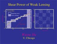
Cosmic Shear
• On even larger scales, the large-scale structure weakly shears
background images: weak lensing

Dark Energy
• Distance redshift relation depends on energy density components
H0D(z) = dz H0
H(a)
• SN dimmer, distance further than in a matter dominated epoch
• Hence H(a) must be smaller than expected in a matter only
wc = 0 universe where it increases as (1 + z) 3/2
H0D(z) =
dze d ln a 3
2 (1+wc(a))
• Distant supernova Ia as standard candles imply that wc < −1/3 so
that the expansion is accelerating
• Consistent with a cosmological constant that is ΩΛ = 0.74
• Coincidence problem: different components of matter scale
differently with a. Why are two components comparable today?

Cosmic Census
• With h = 0.71 and CMB Ωmh 2 = 0.133, Ωm = 0.26 - consistent
with other, less precise, dark matter measures
• CMB provides a test of DA = D through the standard rulers of the
acoustic peaks and shows that the universe is close to flat Ω ≈ 1
• Consistency has lead to the standard model for the cosmological
matter budget:
• 74% dark energy
• 26% non-relativistic matter (with 83% of that in dark matter)
• 0% spatial curvature