Construction of Hyperkähler Metrics for Complex Adjoint Orbits

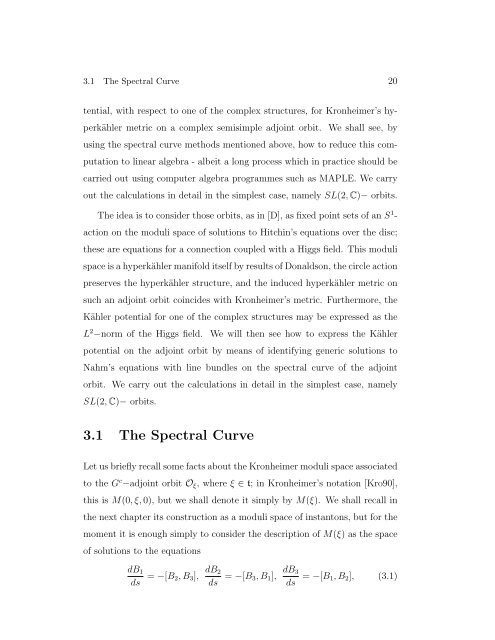
3.1 The Spectral Curve 20
tential, with respect to one of the complex structures, for Kronheimer’s hy-
perkähler metric on a complex semisimple adjoint orbit. We shall see, by
using the spectral curve methods mentioned above, how to reduce this com-
putation to linear algebra - albeit a long process which in practice should be
carried out using computer algebra programmes such as MAPLE. We carry
out the calculations in detail in the simplest case, namely SL(2, C)− orbits.
The idea is to consider those orbits, as in [D], as fixed point sets of an S 1 -
action on the moduli space of solutions to Hitchin’s equations over the disc;
these are equations for a connection coupled with a Higgs field. This moduli
space is a hyperkähler manifold itself by results of Donaldson, the circle action
preserves the hyperkähler structure, and the induced hyperkähler metric on
such an adjoint orbit coincides with Kronheimer’s metric. Furthermore, the
Kähler potential for one of the complex structures may be expressed as the
L 2 −norm of the Higgs field. We will then see how to express the Kähler
potential on the adjoint orbit by means of identifying generic solutions to
Nahm’s equations with line bundles on the spectral curve of the adjoint
orbit. We carry out the calculations in detail in the simplest case, namely
SL(2, C)− orbits.
3.1 The Spectral Curve
Let us briefly recall some facts about the Kronheimer moduli space associated
to the G c −adjoint orbit Oξ, where ξ ∈ t; in Kronheimer’s notation [Kro90],
this is M(0, ξ, 0), but we shall denote it simply by M(ξ). We shall recall in
the next chapter its construction as a moduli space of instantons, but for the
moment it is enough simply to consider the description of M(ξ) as the space
of solutions to the equations
dB1
ds = −[B2, B3], dB2
ds = −[B3, B1], dB3
ds = −[B1, B2], (3.1)