Modeling and Control of Direct Driven PMSG for Ultra Large Wind ...

Abstract—This paper focuses on developing an integrated
reliable and sophisticated model for ultra large wind turbines And to
study the performance and analysis of vector control on large wind
turbines. With the advance of power electronics technology, direct
driven multi-pole radial flux PMSG (Permanent Magnet Synchronous
Generator) has proven to be a good choice for wind turbines
manufacturers. To study the wind energy conversion systems, it is
important to develop a wind turbine simulator that is able to produce
realistic and validated conditions that occur in real ultra MW wind
turbines. Three different packages are used to simulate this model,
namely, Turbsim, FAST and Simulink. Turbsim is a Full field wind
simulator developed by National Renewable Energy Laboratory
(NREL). The wind turbine mechanical parts are modeled by FAST
(Fatigue, Aerodynamics, Structures and Turbulence) code which is
also developed by NREL. Simulink is used to model the PMSG, full
scale back to back IGBT converters, and the grid.
Keywords—FAST, Permanent Magnet Synchronous Generator
(PMSG), TurbSim, Vector Control and Pitch Control
W
I. INTRODUCTION
IND is a promising source of energy. In worldwide there are
now many thousands of wind turbines operating, with a
total nameplate capacity of 196,630MW [1]. There are many
configurations of generating schemes in wind turbines. The
two most interesting configurations are DFIG (Doubly Fed
Induction Generator) with partially 30% back to back
converters and the direct driven PMSG with full scale power
converters. Many papers [2; 3] have proven that the direct
driven PMSG is a good choice due to the elimination of
gearbox, the advances in power electronics technology, the
higher efficiency of PMSG and the wide range of speed
control in the PMSG.The full scale power converters are
divided into generator and grid side converters. The generator
side converter is used mainly to control the electrical torque of
the generator to obtain the optimum power. The grid side
converter is used mainly to control the dc bus voltage and the
reactive power flow to the grid. In this paper vector control is
used to control the two converters.The work in this paper can
be divided into three parts. The first part focuses in modeling
of each part of the system starting with the wind simulator, the
wind turbine, the generator, the converters and ending with the
Ahmed M. Hemeida, teaching assistant with Cairo University, Faculty of
Engineering, Electrical Power and Machines department; (e-mail:
a.hemeida@live.com).
Wael A. Farag , Assistant Professor with Cairo University, Faculty of
Engineering, Electrical Power and Machines department; (e-mail:
wafarag@gmail.com).
Osama A. Mahgoub, Profeesor with Cairo University, Faculty of
Engineering, Electrical Power and Machines department; (e-mail:
mahgoub04@yahoo.com). .
World Academy of Science, Engineering and Technology 59 2011
Modeling and Control of Direct Driven PMSG
for Ultra Large Wind Turbines
Ahmed M. Hemeida, Wael A. Farag, and Osama A. Mahgoub
918
grid. Second part explains the control of each part of this
system. The third part discusses the simulation results.
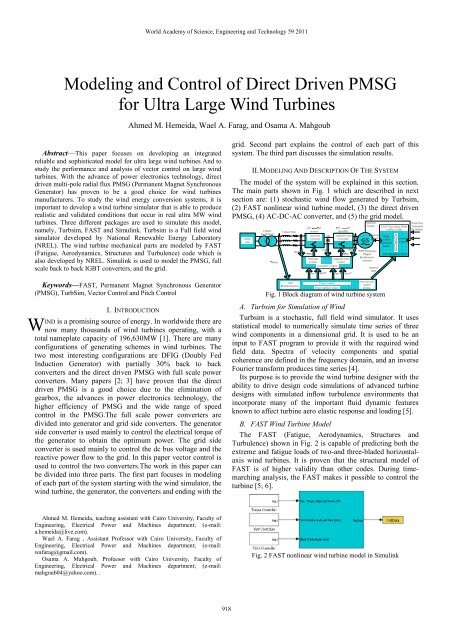
II. MODELING AND DESCRIPTION OF THE SYSTEM
The model of the system will be explained in this section.
The main parts shown in Fig. 1 which are described in next
section are: (1) stochastic wind flow generated by Turbsim,
(2) FAST nonlinear wind turbine model, (3) the direct driven
PMSG, (4) AC-DC-AC converter, and (5) the grid model.
Fig. 1 Block diagram of wind turbine system
A. Turbsim for Simulation of Wind
Turbsim is a stochastic, full field wind simulator. It uses
statistical model to numerically simulate time series of three
wind components in a dimensional grid. It is used to be an
input to FAST program to provide it with the required wind
field data. Spectra of velocity components and spatial
coherence are defined in the frequency domain, and an inverse
Fourier transform produces time series [4].
Its purpose is to provide the wind turbine designer with the
ability to drive design code simulations of advanced turbine
designs with simulated inflow turbulence environments that
incorporate many of the important fluid dynamic features
known to affect turbine aero elastic response and loading [5].
B. FAST Wind Turbine Model
The FAST (Fatigue, Aerodynamics, Structures and
Turbulence) shown in Fig. 2 is capable of predicting both the
extreme and fatigue loads of two-and three-bladed horizontalaxis
wind turbines. It is proven that the structural model of
FAST is of higher validity than other codes. During timemarching
analysis, the FAST makes it possible to control the
turbine [5; 6].
Fig. 2 FAST nonlinear wind turbine model in Simulink

FAST model gives the accessibility to control the generator
torque, the pitch angle, the yaw angle of the nacelle, the high
speed shaft (HSS) brake and deploying the tip brakes. All
these controllers can be implemented in Simulink.
An interface has also been developed between FAST and
Simulink with Matlab enabling users to implement advanced
controls in Simulink convenient block diagram form. The
FAST subroutines have been linked with a Matlab standard
gateway subroutine in order to use the FAST equations of
motion in an S-Function that can be incorporated in a
Simulink model [7].
The wind turbine block, as shown in Fig. 3, contains the S-
Function block with the FAST motion equations. It also
contains blocks that integrate the degree of freedom
accelerations to get velocities and displacements [7].
Fig. 3 FAST wind turbine S-function
To support concept studies aimed at assessing large wind
technology, NREL developed the specifications of a
representative utility-scale multimegawatt turbine now known
as the “NREL offshore 5-MW baseline wind turbine” [6]
which is dedicated for the 5MW wind turbine. This wind
turbine is a conventional three-bladed upwind variable-speed
variable blade-pitch-to-feather-controlled turbine. To create
the model, they obtained some broad design information from
the published documents of turbine manufacturers, with a
heavy emphasis on the REpower 5MW machine.
The specifications of the 5MW wind turbine is shown in
Appendix [6].
The output power of wind turbine can be defined as the
difference between the power in the moving air before and
after the rotor [8];
1 2 3
P wt = ρπR VwC
p ( λ,
β )
(1)
2
where ρ represents the air density, Vw represents the wind
speed, R represents the blade radius, and Cp represents the
power coefficient. The maximum value of Cp is between 0.4
and 0.5 which is less than Betz’s limit 0.59. The value of Cp is
function of tip speed ratio λ and pitch angle β.
ω * R
λ =
(2)
Vw
where ωm is the rotational speed (rad/sec).
The rotor torque can be expressed as;
T
wt
1 2 3
R Vw
ρπ Cp
( λ,
β )
= 2
ω
and the electro mechanical equation of the system can be
expressed as:
dω
Twt − Te
= J
(4)
dt
World Academy of Science, Engineering and Technology 59 2011
m
(3)
919
where Te the electromagnetic torque of the generator and J
is the inertia of the system.
C. 5MW Direct Driven PMSG Modeling
1) Machine Equivalent Model
Before obtaining the equivalent model of the radial flux
PMSG in Fig. 4, it is necessary to calculate the total
number of poles and introduce constraints on the leakage ratio
of the machine. The equivalent model will then be derived in
terms of number of stator conductors, Ns based on the physical
construction of the machine described in [9], yielding the
induced voltage, Epm, the synchronous inductance, Ls, and the
stator resistance, Rs from equations described in [10; 14].
Finally, parameters and machine equations are transposed in
the rotor reference frame. This is more illustrated in [9; 10;
11].
Fig. 4 Electrical diagram in terms of N s
The data for the PMSG is shown in Appendix.
2) General Equations
The back e.m.f Epmln max produced by the magnets depends
on the mechanical rotational speed ωm(rad/sec). This is
illustrated in the following equations;
max
ln = ω e * pm
(5)
Epm ϕ
where ωe is the electrical rotational speed (rad/sec) and ϕpm
is the flux linkage established by magnets (V.S).
ω = P * ω
(6)
e
m
where P = number of pole pairs.
3) Dqo Equations
Almost all drive systems use the dynamic dqo model of a
machine. This converts the 3 phase ac quantities to dc
quantities, which can be easily controlled by a simple
proptional integral (PI) controller. The transformation from 3
phase variables with time varying (abc) frame to stationary
dq0-frame defined in Fig. 5 [12].
Fig. 5 Synchronization for the rotor position for the park
transformation
Machine equations based on the rotor reference position are
described in Equations (7) and (8) and they are marked with
the subscript “r”.
r
r r dIq
r
Vq −RsI
q − Lq
− ω rLd
Id
+ ωrϕ
pm
dt
= (7)
r r dI
r
Vd = −Rs
I d − Ld
+ ωr
Lq
I q (8)
dt
r
d

The Variables Rs, Ld and Lq are the stator resistance, direct
and quadrature inductance respectively of permanent magnet
synchronous generator, where Ld = Lq = Ls.
Fig. 6 shows the equivalent circuit of the PMSG in d-q axis.
The electrical torque is shown in equation (9). It is clear that to
control the electrical torque the q-axis current can be
controlled.
3 r
Te Pϕ
pmIq
2
= (9)
Fig. 6 Equivalent circuit of PMSG in d-q reference frame
D. Converter Model
The back-to-back converter is composed by a forcecommutated
rectifier and a force-commutated inverter as
shown in Fig. 7 each is composed of six insulated gate bipolar
transistor (IGBT) connected with a common DC-link.
An advantage of this system is the dc link capacitor which
decouples the two converters and a separate control on each
converter can be used.
Fig. 7 Structure of the back to back voltage source converter (VSC)
A drawback of this system is the increase of the switching
losses and also the presence of the DC-Link capacitor since it
is bulky and heavy. It increases the cost and may be of most
importance. This reduces the overall life time of the system
[13]. The equivalent circuit of a voltage source converter is
shown in Fig. 8.
Fig. 8 Equivalent circuit of voltage source converter with ideal switch
The DC current Idc is expressed as;
I dc ( ha
( t)
Ia
+ hb
( t)
Ib
+ hc
( t)
Ic
)
= (10)
where ha(t), hb(t) and hc(t) are the switching status of the
switches in VSC.
The output phase voltages are expressed by the following
equation, which are dependent on ha(t), hb(t) and hc(t).
⎡Van
⎤ ⎡ 2
⎢ ⎥ V ⎢
⎢V
⎥ = dc
bn ⎢
−1
3
⎢ ⎥
⎣Vcn
⎦
⎢
⎣−1
−1
2
−1
−1⎤⎡ha
( t)
⎤
⎥⎢
⎥
−1
⎥⎢hb
( t)
⎥
2 ⎥
⎦
⎢ ⎥
⎣hc(
t)
⎦
(11)
This topology is used for full rating power converter in
some large scale wind turbines [14; 15].
World Academy of Science, Engineering and Technology 59 2011
920
E. Grid Model
The grid can be represented as shown in Fig. 9. The output
of the coupling is represented by subscript U and grid voltage
is represented by subscript E.
The voltage equation per phase can be described as follows:
dI
E = U + Rs
* I + Ls
*
(12)
dt
where Rs and Ls represent the equivalent series resistance
and inductor of the filter and transformer between grid and
inverter output.
Fig. 9 Grid Side Converter
For a three phase voltages with a rotating frame angle Ө
which starts rotating with phase a, the amplitude of the phase
voltages of the grid (Ean, Ebn, Ecn) which equals Es will be
placed on the d- axis (Ed = Es). The q-axis component voltage
will be zero. Then converting Equation (12) to d-q frame
results in the following equations;
r
r r dIq
r
Vq = RsIq
+ Lq
+ ω rLd
Id
+ 0
(13)
dt
r
r r dI r
V d
d = RsI
d + Ld
− ω rLq
Iq
+ Es
(14)
dt
where Vd r and Vq r are the d-q output voltages of the
inverter, ωr is the grid frequency in rad/sec, Ld and Lq are the
inductance in d-q axis which equal Ls and Id r and Iq r are the
d-q axis currents.
The equations of active and reactive power converted to
grid are shown in Equations (15), (16). It’s shown that to
control active power the d-axis current must be controlled and
to control reactive power the q-axis current is needed to be
controlled as shown in the following equations.
3
P Es
* Id
2
= (15)
3
Q Es
* Iq
2
= (16)
The data for the grid configuration is shown in Appendix.
III. CONTROL OF PMSG BASED WIND TURBINES
The requirements of any turbine control system are to
extract almost all the output power of the wind turbine. Four
regions can be defined for the control of the wind turbine as
shown in Fig. 10.
In region 1, the output power from the wind turbine is too
low, this won’t be sufficient to operate the wind turbine.
Region 1.5 is a linear transition between regions 1 and 2.
This starts from 6.9 rpm and ends at 30% above the starting
rotor speed.

In region 2, the controller is adjusted to extract almost all
the output power available in the wind turbine. This is done by
changing the electromagnetic torque of the generator to
always work on maximum power coefficient. This region ends
at 99% of the rated rotor speed. This is done by the generator
side converter and this is more illustrated in Section III.A.
Region 2.5 is a linear transition between regions 2 and 3.
This region is required to limit tip speed at rated power. This
region ends at rated rotor speed.
In region 3, the generator electromagnetic torque is kept
constant and the pitch angle is adjusted to keep the rotor speed
constant at its nominal value. Therefore, the output power is
kept constant.
Fig. 10 Power curve for wind turbine
A. Generator Side Converter Control
Type of control used is field oriented control (FOC) as
shown in
Fig. 11. This type of control gives high performance. FOC
uses the shaft speed, obtained by an encoder as a feedback in
the control strategy.
The d and q axis current component represents the
components of flux and torque. The torque and flux can be
controlled separately for the current control loops.
Constant Torque Angle Control (CTA) is the control
technique used to control the d and q axis currents. CTA keeps
the torque angle constant (angle between the stator current
vector and the rotor permanent magnet flux) at 90 ° . This is
done by keeping the stator current reference in d-axis at zero,
to produce maximum torque per ampere; therefore the
resistive losses are minimized. The stator current reference in
q-axis is calculated from the reference torque using Equation
(9) [16].
The required d-q components of the voltage vector are
derived from two PI current controllers. After the PI current
controllers, compensation terms in the following two
equations are added to improve the transient response. They
are obtained from Equations (7) and (8).
r
Component → 1 = ωrLq
Iq
(17)
r
Component 2 = −ω
rLd Id
+ ωr
* ϕ pm
→ (18)
Space Vector Modulation (SVM) is the technique used to
create the duty cycles of the desired reference voltages. The
PWM switching signals for the power converter switching
devices can be obtained by comparing the duty cycles with the
carrier signal in order to create. The PI parameters are
designed using sisotool in MATLAB as described in [17].
World Academy of Science, Engineering and Technology 59 2011
921
Fig. 11 Generator Side Control
The reference of the electromagnetic torque Tem * can be
calculated by using optimal torque control method [18]. This
control method uses the measured rotational speed (rad/sec) of
the shaft and the parameters of the wind turbine to obtain the
optimal operating point. The output wind turbine power is
obtained from Equation (3).
1 2 3 1 C p(
λ,
β ) 5 3
Pwt ρπ R VwCp
( λ,
β ) =
ρπR
ω
2
2 3
m
λ
= (19)
By replacing λ(t) by λopt and Cp(λ,β) = Cp(λopt,β), the
reference power can be obtained in region 2.
Pwtopt where;
3
Kωm
= (20)
1 C p(
λ,
β ) 5
K = ρπR
2 3
λ
rad 2
N.
m /( )
sec
(21)
The reference torque is calculated as follows;
Twtopt 2
Kωm
= (22)
The value of K for the 5MW wind turbine system is
23342.87N.m/rpm 2 .
B. Pitch Angle Control
The basic aim of pitch control scheme is to keep constant
rated power at region 3. Blade pitch actuator for the 5MW
wind turbine has a maximum rate limit of 8 degree/sec. Also,
the minimum and maximum blade pitch settings are 0° and
90° respectively [6]. The blade pitch actuator is a second order
system with a very high natural frequency of 30Hz and a
damping ratio of 2% [6].
Fig. 12 shows the control scheme for pitch system. The
rotational speed is kept constant at rated speed by increasing
pitch angle. This will reduce the aerodynamic torque produced
by the wind turbine. Below rated rotor speed the pitch angle is
adjusted at its lower limit.
The PI gains are designed by linearizing the FAST model at
wind speed of 18m/sec and by using sisotool in Matlab the
gains are obtained.
Fig. 12 Pitch Angle Control Scheme

C. Grid Side Converter Control
The aim of the control as shown in
Fig. 13 is to transfer all the active power produced by the
wind turbine to the grid and also to produce no reactive power
so that unity power factor is obtained, unless the grid operator
requires reactive power compensation. In
Fig. 13 the phase locked loop (PLL) is used to synchronize
the three phase voltage with the grid voltage. The main aim of
the controller is to:
• Regulate the DC bus voltage constant to be greater than the
amplitude of the grid line to line voltage. This is done by
controlling the d-axis current component. So, if turbine Power
Pt and generator power Pg are equal, Vdc must be constant.
dVdc
Pt
Pg
Ic C = −
dt Vdc
Vdc
= (23)
where Ic is the capacitor current.
• Control the reactive power through the q current component
as can be concluded from Equation (16).
A compensation terms mentioned in the following
equations, will be added to improve the transient response of
the system which can be concluded from Equations (13) and
(14).
r
Component → 1 = −ωr
LqI
q + Es
(24)
r
Component → 2 = ωrLd
Id
(25)
Fig. 13 Grid Side Converter Control
IV. SIMULATION RESULTS
The system is tested under two conditions. The first
condition with the wind speed changes in steps. The pitch
angle response for step changes for wind speed is shown in
Fig. 14. The wind is changing from 12 to 20m/sec in 1m/sec
steps. It is also observed that the rotor speed raises only 5% of
the rated value. The power has an average value of 0.998p.u
over the time period of 100sec. These values are within
reasonable range.
World Academy of Science, Engineering and Technology 59 2011
922
Fig. 14 Pitch angle response for step changes in wind speeds
Under the second condition a stochastic wind speed
generated by Turbsim [4] will be used. The controller is tested
with wind profile named great planes wind profile (GP_LLJ).
This wind profile is standard, validated by IEC, and has a
coherent structure. The hub height wind speed is shown in Fig.
15 with an average value of 18m/sec and a standard deviation
of 1.15. It is shown that the rotor speed changes within 5% of
the rated value. This value is within reasonable range. The
power has an average value of 0.92p.u over the time period of
100sec.
Fig. 15 Pitch angle response for stochastic wind speeds
A. Generator and Grid Side Control
Two cases will be studied in this study. In the first case the
generator and grid side controller are tested under wind speed
steps of 2m/sec from 6 to 10m/sec as shown in Fig. 16.
Fig. 16 Speed, electromagnetic torque and dc bus voltage response
for wind speed variations
For every increase in wind speed the wind turbine
aerodynamic torque increases and correspondingly the
electromagnetic torque increases. The rotor speed also

increases and settles after duration of 5sec. This is due to the
large inertia of the system. The dc bus voltage is set to be at
1.6p.u. It is also observed that the dc bus voltage isn’t affected
by the variations of wind speed. This is due to the electrical
system response is very fast compared to the mechanical time
constant.
Fig. 17 a and b show the d and q-axis responses for the
generator currents. The generator d-axis current is set all over
the simulation to zero to get the maximum torque/ampere and
the q-axis is directly tracking the electromagnetic torque. The
ripple is around 2%.
Fig. 17 c and d show the d and q-axis responses for the grid
currents. The grid q-axis current is set all over the simulation
to zero to get zero reactive power and the d-axis component is
directly tracking the power flow from the turbine to the grid.
The ripple in the d-axis current is around 4%. But in the case
of the q-axis it increases to 10%.
Fig. 18 shows the phase a current of the grid for 10 cycles.
It shows a THD of 3.76% which is quite acceptable.
Fig. 17 D and Q axis currents response for generator and grid
Fig. 18 Phase A Grid Current.
In the second case the controller is tested under turbulence
wind which has a mean wind speed of 9.2m/sec, standard
deviation of 0.381 and a power law exponent of 0.143 as
shown in Fig. 19. The wind speed has stochastic wind
variations. It varies about a mean value of 9m/sec. The rotor
speed increases at first then it reaches a steady state value.
Whenever the wind speed variations about the mean wind
World Academy of Science, Engineering and Technology 59 2011
speed the system doesn’t sense these variations due to the
large inertia of the rotor. The generator is only affected by the
mean wind speed.
Fig. 19 Speed, electromagnetic torque and dc bus voltage response
for wind speed variations
V. CONCLUSION
The main objective of this paper was the modeling and
simulation of the ultra large wind turbine system using
validated models of wind turbine mechanical and electrical
systems. Then the electrical system consisting of the
generator, back to back VSC and the grid have been described
mathematically component by component. Then the
performance and analysis of vector control and the pitch
control algorithms have been studied on the system. The
simulation was conducted under conditions of step wind
speeds and stochastic wind flow generated by TurbSim. The
simulation results have shown the correct functioning of the
controllers applied on each component in the whole system.
APPENDIX
PROPERTIES FOR THE NREL 5-MW BASELINE WIND
TURBINE
Wind Turbine Parameters
Rating 5MW
Rotor Orientation, Configuration Upwind, 3 Blades
Control Variable Speed,
Collective Pitch
Rotor and turbine inertia about the
shaft
2
38,759,228 Kg .m
Generator Parameters
Nominal Power Pgen,nom
5.3MW
Nominal Torque Tgen,nom
4.18MN.m
Generator inertia about the shaft 5,025,500 Kg .m
2
Generator Side Characteristics
Parameters Value
No. of pair poles, P. 100
The r.m.s induced no load voltage at
rated speed, Epmln rms .
2.31KV
The stator resistance, Rs. 0.08Ω
The magnetizing inductance, Lsm. 3.352mH
The leakage inductance, Lsl. 5.028mH
Grid Side Characterstics
Parameters Value
Grid Voltage. 4KV
923

Line filter inductance. 4mH
DC bus voltage. 6.4KV
DC bus capacitance. 4000µF
ACKNOWLEDGMENT
This project has been funded by the Science and
Technology Development Fund (STDF) project number 1411.
REFERENCES
[1] Association, World Wind Energy. World Wind Energy Report. Cairo,
Egypt : World Wind Energy Association WWEA 2011, 31 October.
[2] H. Polinder, F.F.A. van der Pijl, G.J. de Vilder, P. Tavner, “Comparison
of direct-drive and geared generator concepts for wind turbines”, IEEE
Trans. Energy Conversion, Vol. 21, pp. 725-733, September 2006.
[3] D. Bang, H. Polinder, G. Shrestha, and J.A. Ferreira, “Review of
generator systems for direct-drive wind turbines”, in Proc. EWEC
(European Wind Energy Conference & Exhibition,) Brussels, Belgium,
March 31 - April 3, 2008.
[4] J. Jonkman, B.J. “Turbsim user’s guide”. s.l. : NREL/TP-500-46198:
National Renewable Energy Laboratory., August 2009.
[5] Sayooj B Krishna, Reeba S V. “Simulation Of Wind Turbine With
Switched Reluctance Generator by FAST and Simulink”. .November
2009, National Conference on Technological Trends.
[6] J. Jonkman, S. Butterfield, W. Musial, and G. Scott. “Definition of a 5-
MW Reference Wind Turbine for Offshore System Development”. s.l. :
NREL, February 2009.
[7] J. Jonkman, B.J. “FAST User’s Guide, Technical Report”. s.l. :
NREL/EL-500-38230: National Renewable Energy Laboratory., August,
2005.
[8] Cristian Busca, Ana-Irina Stan, Tiberiu Stanciu and Daniel Ioan Stroe.
“Control of Permanent Magnet Synchronous of large wind turbines”.
Denmark : Departament of Energy Technology: Aalborg University,
November 2010, Industrial Electronics (ISIE), ieee, pp. 3871 - 3876 .
[9] D. Bang, H. Polinder, J.A. Ferreira. “Design of Transverse Flux
Permanent Magnet Machines for Large Direct-Drive Wind Turbines”.
Electrical Power Processing / DUWIND, Delft University of
Technology. Netherlands : Delft University of Technology, 2010. phD
Thesis.
[10] Hui Li, Zhe Chen. “Design Optimization and Evaluation of Different
Wind Generator Systems”. February 2009, Sustainable Power
Generation and Supply, 2009. SUPERGEN '09.
[11] Li, Hui, Chen, Zhe and Polinder, H. “Optimization of multibrid
permanent-magnet wind generator systems”. Security & New Technol.,
Chongqing Univ : IEEE Transactions on Energy conversion, March
2009, IEEE Transactions on Energy conversion , Vol. 24, pp. 82-92.
[12] P. C. Krause, O. Wasynczuk, and S. D. Sudho. “Analysis of Electric
Machinery and Drive System”s. s.l. : John Wiley & Sons, , 2002.
[13] Floren lov, FredeBlaabjerg. “Power electronics Control of wind energy
in distributed power systems”. Department of energy technology,
Aaloborg university. 2009. pp. 1–16.
[14] Shuhui Li, Timothy A.Haskew, Ling Xu. “Conventional and novel
control designs for direct driven PMSG wind turbines”. 3, March 2010,
Electric Power Systems Research, Vol. 80, pp. 328-338.
[15] Remus Teodorescu, Pedro Rodriguez. “Thesis in Reactive power control
for wind power plant with STATCOM”. Institute of Energy Technology-
Pontoppidanstræde 101. 2010. Master thesis.
[16] Busca, C., et al., et al. “Vector control of PMSG for wind turbine
applications”. s.l. : Dept. of Energy Technol., Aalborg Univ., Aalborg,
Denmark , 2010 , Industrial Electronics (ISIE), pp. 3871 - 3876 .
[17] Andreea Cimpoeru, Kaiyuan Lu. “Encoderless Vector Control of PMSG
for wind turbine applications”. Institute of Energy Technology, Institute
of energy technology. s.l. : AALBORG University, 2010. Master Thesis.
[18] Michael J. Grimble, Professor Michael A. Johnson. “Optimal Control of
Wind Energy Conversion Systems”. August 2007 .
World Academy of Science, Engineering and Technology 59 2011
924