Baire Category, Probabilistic Constructions and Convolution Squares
Baire Category, Probabilistic Constructions and Convolution Squares
Baire Category, Probabilistic Constructions and Convolution Squares

You also want an ePaper? Increase the reach of your titles
YUMPU automatically turns print PDFs into web optimized ePapers that Google loves.
<strong>Baire</strong> <strong>Category</strong>, <strong>Probabilistic</strong> <strong>Constructions</strong><br />
<strong>and</strong> <strong>Convolution</strong> <strong>Squares</strong><br />
Contents<br />
T. W. Körner<br />
August 13, 2009<br />
1 Introduction 2<br />
2 <strong>Baire</strong>’s theorem 3<br />
3 The Hausdorff metric 6<br />
4 Independence <strong>and</strong> Kronecker sets 10<br />
5 Besicovitch Sets 14<br />
6 Measures 18<br />
7 A theorem of Rudin 20<br />
8 The poor man’s central limit theorem 24<br />
9 Completion of the construction 28<br />
10 Sets of uniqueness <strong>and</strong> multiplicity 35<br />
11 Distributions 42<br />
12 Debs <strong>and</strong> Saint-Reymond 43<br />
13 The perturbation argument 47<br />
14 <strong>Convolution</strong> of distinct measures 51<br />
15 The Wiener–Wintner theorem 54<br />
1
16 Hausdorff dimension <strong>and</strong> measures 58<br />
17 Thick Wiener–Wintner measures 67<br />
18 More probability 70<br />
19 Point masses to smooth functions 77<br />
20 Hausdorff dimension <strong>and</strong> sums 86<br />
21 The final construction 89<br />
22 Remarks 94<br />
1 Introduction<br />
In the past few years I have written a number of papers using simple <strong>Baire</strong><br />
category <strong>and</strong> probabilistic results. The object of this course is to give examples<br />
of the main theorems <strong>and</strong> the methods used to obtain them.<br />
Although we shall obtain other results, our main concern will be the<br />
question. Knowing something about the measure µ, what can we say about<br />
its convolution with itself (that is to say, the convolution square) µ ∗µ? This<br />
question goes back at least as far as the paper of Wiener <strong>and</strong> Wintner [28]<br />
in which they show that the convolution square of a singular measure need<br />
not be singular.<br />
Those who already know about such things may find it useful to see some<br />
of our main results. Those who do not, should be reassured that we will<br />
provide appropriate definitions <strong>and</strong> background in due course. We give a<br />
new proof of the following theorem of Besicovitch.<br />
Theorem 5.4. There exists a closed bounded set of Lebesgue measure containing<br />
lines of length at least 1 in every direction.<br />
We prove a quantitive verision of a theorem of Rudin.<br />
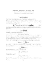
Theorem 7.3. Suppose that φ : N → R is a sequence of strictly positive<br />
numbers with r α φ(r) → ∞ as r → ∞ whenever α > 0. Then there exists a<br />
probability measure µ such that φ(|r|) ≥ |ˆµ(r)| for all r = 0, but suppµ is<br />
independent.<br />
We prove an extension (found independently by Matheron <strong>and</strong> Zelen´y)<br />
of a celebrated theorem of Debs <strong>and</strong> Saint Reymond.<br />
Theorem 12.5. Let B be a set of first category in T. Then we can find<br />
a probability measure µ with ˆµ(r) → 0 as |r| → ∞ such that suppµ is<br />
2
independent <strong>and</strong> the subgroup G of T generated by suppµ satisfies<br />
G ∩ B ⊆ {0}.<br />
We produce two substantial extensions of the theorem of Wiener <strong>and</strong><br />
Wintner. The first is related to the theorem of Debs <strong>and</strong> Saint Reymond.<br />
Theorem 15.1. Let A be a set of first category in T. Then we can find a<br />
probability measure µ such that suppµ∩A = ∅ but d(µ ∗µ)t = f(t)dt where<br />
f is a Lebesgue L 1 function.<br />
The second further extends a result of Saeki.<br />
Theorem 17.4. If 1 > α > 1/2, then there exists a probability measure µ<br />
such that the Hausdorff dimension of the support of µ is α <strong>and</strong> d(µ ∗ µ)(t) =<br />
f(t)dt where f is Lipschitz α − 1<br />
2 .<br />
We conclude with a result on Hausdorff dimension.<br />
Theorem 20.1. Given a sequence αj with 0 ≤ αj ≤ αj+1 < 1, we can find<br />
a closed set E such that<br />
E[j] = E + E + ... + E<br />
<br />
j<br />
has Hausdorff dimension αj for each j ≥ 1.<br />
Any course like this is is bound to be rather uneven in difficulty <strong>and</strong> I have<br />
chosen to accentuate this unevenness by spending a substantial amount of<br />
time discussing well known <strong>and</strong> relatively easy results. The beginner should<br />
concentrate on these discussions, leaving the technical (<strong>and</strong>, I am afraid<br />
still imperfectly digested) details of my own arguments to a hypothetical<br />
interested expert.<br />
2 <strong>Baire</strong>’s theorem<br />
The study of complete metric spaces enables us to replace certain recurring<br />
arguments by general principles. One of the most important of the principles<br />
is given by <strong>Baire</strong>’s category theorem.<br />
Theorem 2.1. [<strong>Baire</strong>’s category theorem] Let (X,d) be a non-empty<br />
complete metric space. If E1, E2, ...are closed subsets of X with dense<br />
complements, then ∞<br />
j=1 Ej is non-empty.<br />
<strong>Baire</strong>’s theorem may be restated as follows.<br />
3
Theorem 2.2. Let (X,d) be a non-empty complete metric space. Suppose<br />
that Pj is a property such that:-<br />
(i) The property of being Pj is stable in the sense that, given x ∈ X<br />
which has property Pj, we can find an ǫ > 0 such that whenever d(x,y) < ǫ<br />
the point y has the property Pj.<br />
(ii) The property of not being Pj is unstable in the sense that, given<br />
x ∈ X <strong>and</strong> ǫ > 0, we can find a y ∈ X with d(x,y) < ǫ which does not have<br />
the property Pj.<br />
Then there is an x0 ∈ X which has all of the of the properties P1, P2,<br />
....<br />
Proof of equivalence of Theorems 2.1 <strong>and</strong> 2.2. Let x have the property Pj if<br />
<strong>and</strong> only if x /∈ Ej. <br />
It is unlikely that anyone who reads these notes is unfamiliar with Theorem<br />
2.1 or its proof, but I include a proof for completeness. We shall prove<br />
a slightly stronger version of <strong>Baire</strong>’s theorem.<br />
Theorem 2.3. Let (X,d) be a complete metric space. If E1, E2, ...are<br />
closed sets with empty interiors, then X \ ∞<br />
j=1 Ej is dense in X.<br />
Proof. Suppose that x0 ∈ X <strong>and</strong> δ0 > 0. We shall show that there exists a<br />
y ∈ B(x0,δ0) such that y /∈ ∞ j=1 Ej.<br />
To this end, we perform the following inductive construction. Given<br />
xn−1 ∈ X <strong>and</strong> δn > 0, we can find xn ∈ X such that xn ∈ B(xn−1,δn/4), but<br />
xn /∈ En. (For, if not, we would have B(xn−1,δn−1/4) ⊆ En <strong>and</strong> En would<br />
have a non-empty interior.) Since En is closed <strong>and</strong> xn /∈ En we can now find<br />
a with δn−1/2 > δn > 0 such that B(xn,δn) En = ∅.<br />
Now observe that<br />
δm ≤ 2 −1 δm−1 ≤ 2 −2 δm−2 ≤ ...2 n−m δn<br />
for all m ≥ n ≥ 0. It follows that, if r ≥ s<br />
s−1<br />
d(xr,xs) ≤<br />
j=r<br />
d(xj+1,xj) ≤<br />
s−1<br />
δr/4 ≤ 4 −1 s−1<br />
δ0<br />
j=r<br />
j=r<br />
2 −r ≤ 2 −r−1 δ0.<br />
Thus the xr form a Cauchy sequence <strong>and</strong> converges in (X,d) to some point<br />
y.<br />
The same kind of calculation as in the last paragraph gives<br />
s−1<br />
d(xr,xs) ≤<br />
j=r<br />
d(xj+1,xj) ≤<br />
s−1<br />
δr/4 ≤ 4 −1 δr<br />
j=r<br />
4<br />
s−r−1 <br />
j=0<br />
2 −r ≤ δr/2,
whenever s ≥ r <strong>and</strong> so<br />
d(xr,y) ≤ d(xr,xs) + d(xs,y) ≤ δr/2 + d(xs,y) → δr−1/2<br />
as s → ∞. We thus have d(xr,y) ≤ δr/2 so y ∈ B(x0,δr) <strong>and</strong> y /∈ Er for<br />
each r ≥ 1 as required. <br />
For historical reasons <strong>Baire</strong>’s category theorem is associated with some<br />
rather peculiar nomenclature.<br />
Definition 2.4. Let (X,d) be a metric space. We say that a a subset A of X<br />
is of the first category if it is a subset of the union of a countable collection<br />
of closed sets with empty interior 1 . We say that quasi-all points of X belong<br />
to the complement X \ A of X.<br />
Theorem 2.3 thus states that the complement of a set of the first category<br />
in a complete metric space is dense in that space. The next exercise gives a<br />
simple but very useful property of sets of first category.<br />
Exercise 2.5. Show that the countable union of sets of the first category is<br />
itself a set of the first category.<br />
The reader will have met the following theorem before.<br />
Theorem 2.6. R is uncountable.<br />
Proof. If we give R the usual metric, then point sets {x} are closed <strong>and</strong><br />
have empty interior. It follows that, if E is a countable subset of R, then<br />
E = <br />
e∈E {e} is of first category <strong>and</strong> so E = R. <br />
The st<strong>and</strong>ard undergraduate proof involves decimal expansions but this<br />
proof avoids have to talk about the relation between real numbers <strong>and</strong> decimals.<br />
It is also much closer to Cantor’s original proof.<br />
Exercise 2.7. If (X,d) is a metric space we say that a point x ∈ X is<br />
isolated if we can find a δ > 0 such that B(x,δ) = {x}.<br />
(i) Show that a point x ∈ X is isolated if <strong>and</strong> only if {x} is open.<br />
(ii) Show that any complete non-empty metric space without isolated<br />
points is uncountable.<br />
(iii) Give an example of a complete infinite metric space which is countable.<br />
(vi) Give an example of a uncountable complete metric space with every<br />
point isolated.<br />
1 Some authors, say that A of X is of the first category if it is the union of a countable<br />
collection of closed sets with empty interior. They have history, on their side, but not<br />
common usage.<br />
5
There are several reasons for using the <strong>Baire</strong> category theorem when we<br />
seek examples of particular types of behaviour.<br />
The first is practical. Although any <strong>Baire</strong> category argument can obviously<br />
be replaced by a direct argument, if there are several properties<br />
involved, each of which involves countably many conditions the direct argument<br />
may require quite a lot of notation <strong>and</strong> careful interlocking of several<br />
inductions. Such arguments are not hard to write (<strong>and</strong> indeed may give the<br />
author some pleasure), but are may be hard to read.<br />
The second argument is that a property which holds quasi-always is, in<br />
some sense, generic. The next exercise shows that we must not press this<br />
argument too far.<br />
Exercise 2.8. The following is a well known procedure for constructing ‘Cantor<br />
sets’. Let E0 = [0, 1] <strong>and</strong> let ζ1, ζ2, ... be a sequence of real numbers with<br />
0 < ζj < 1. At the nth stage En is the union of 2 n disjoint closed intervals<br />
I(r,n) all of the same length. We define En to be the union of the 2 n+1 disjoint<br />
closed intervals formed by removing an open interval J(r,n) of length<br />
ζn times the length of the initial interval I(r,n) from the centre of I(r,n).<br />
(Thus if I(r,n) = [cr,n −δn,cr,n +δ] we take J(r,n) = (cr,n −ζnδn,cr,n +ζnδn)<br />
<strong>and</strong><br />
2<br />
En+1 =<br />
n<br />
<br />
(I(r,n) \ J(r,n).<br />
r=1<br />
(i) Explain why ζ = ∞ n=1 ζn is well defined. Show that ζ can take any<br />
value subject only to the condition 1 > ζ ≥ 0.<br />
(ii) Show that E = ∞ n=1 En is a closed nowhere dense set without isolated<br />
points. Show that E has Lebesgue measure ζ.<br />
(iii) Construct a set H ⊆ [0, 1] of first <strong>Baire</strong> category but of Lebesgue<br />
measure 1. Points in H are ‘generic in the the sense of measure theory’<br />
(almost all points in [0, 1] lie in H) but the points of [0, 1] \ H are ‘generic<br />
in the the sense of topology’ (quasi-all points in [0, 1] lie [0, 1] \ H).<br />
(iv) Construct a set P ⊆ R of first <strong>Baire</strong> category such that R \ P has<br />
Lebesgue measure zero.<br />
The third argument is that the act of seeking a <strong>Baire</strong> type proof may, by<br />
itself, suggest a new ways of looking at your problem.<br />
3 The Hausdorff metric<br />
The Hausdorff metric measures the difference between compact sets.<br />
6
Definition 3.1. Let (X,d) be a metric space <strong>and</strong> let E be the collection of<br />
non-empty compact subsets of X. We write<br />
dE(E,F) = sup<br />
e∈E<br />
inf<br />
f∈F<br />
d(e,f) + sup<br />
e∈E<br />
inf<br />
f∈F d(e,f)<br />
for all E, F ∈ E <strong>and</strong> call dE the Hausdorff metric on E.<br />
The proof that the Hausdorff metric is indeed a metric is easy, but not, I<br />
think, trivial. We use the following subsidiary lemma.<br />
Lemma 3.2. Let (X,d) be a metric space <strong>and</strong> let E be the collection of<br />
non-empty compact subsets of X. If we write<br />
for E, F ∈ E then<br />
for all E, F G ∈ E.<br />
∆(E,F) = sup<br />
e∈E<br />
inf<br />
f∈F d(e,f)<br />
∆(E,G) ≤ ∆(E,F) + ∆(F,G)<br />
Proof. Write d(e,F) = inff∈F d(e,f) for e ∈ X <strong>and</strong> F ∈ E. By the triangle<br />
inequality,<br />
d(e,g) ≤ d(e,f) + d(f,g)<br />
so<br />
for all g ∈ G whence<br />
for all f ∈ F. Hence<br />
for all e ∈ E <strong>and</strong><br />
d(e,G) ≤ d(e,f) + d(f,g)<br />
d(e,G) ≤ d(e,f) + d(f,G) ≤ d(e,f) + ∆(F,G)<br />
d(e,G) ≤ d(e,F) + ∆(F,G)<br />
∆(E,G) ≤ ∆(E,F) + ∆(F,G).<br />
Exercise 3.3. Use Lemma 3.2 to show that the Hausdorff metric is indeed<br />
a metric.<br />
Lemma 3.4. (We use the notation of Definition 3.1.) If (X,d) is complete,<br />
then the Hausdorff metric is complete.<br />
7
Proof. It is sufficient to show that, if En ∈ E <strong>and</strong> dE(En,En+1) ≤ 2 −n−1 for<br />
all n ≥ 1, then En converges in the Hausdorff metric.<br />
To this end, let E be the set of e ∈ X such that there exist en ∈ En with<br />
d(en,e)) → 0 as n → ∞. We observe that, if e ∈ E then, given any m, we<br />
can find an n ≥ m + 1 such that d(e,en) < 2 −m . Since<br />
n−1<br />
dE(Em,En) ≤<br />
j=m<br />
<br />
n−1<br />
dE(Ej,Ej+1) ≤ 2 −(j+1) < 2 −m<br />
we can find xm ∈ Em such that d(xm,en) < 2 −m <strong>and</strong> so d(xm,e) < 2 −m+1 .<br />
Thus<br />
E ⊇ {x : d(x,xm) < 2 −m+1 for some x ∈ Em.<br />
We next show that E is compact. Suppose that y(j) ∈ E for j ≥ 1.<br />
We construct infinite subsets An of N as follows. Set A0 = N. If Am−1<br />
has been defined we obtain Am as follows. Since E is covered by open balls<br />
B(x, 2 −m+1 ) with x ∈ Em <strong>and</strong> E is compact, E is covered by a finite set<br />
of such balls <strong>and</strong> one of those balls B(xm, 2 −m+1 ) must contain an infinite<br />
subset of Am. We observe that d(xm,xm+1) < 2 −m so the xm converge to<br />
some y ∈ E. Choose n(j) ∈ Aj so that n(j) → ∞. Then d(yn(j),y) → 0 as<br />
j → ∞. Thus E is compact.<br />
The second paragraph of the proof shows that<br />
j=m<br />
sup inf<br />
f∈En<br />
e∈E d(e,f) ≤ 2−n+1 .<br />
If xn ∈ En then we can find xj ∈ Ej such that d(xj,xj+1) < 2 −j+1 . Since the<br />
xj are Cauchy, they converge to some x. We have x ∈ E <strong>and</strong><br />
so<br />
d(x,xn) ≤<br />
sup<br />
e∈E<br />
inf<br />
∞<br />
d(xj,xj+1) ≤ 2 −n+2<br />
j=n<br />
f∈En<br />
d(e,f) ≤ 2 −n+2 .<br />
Thus dE(En,E) → 0 as n → ∞. <br />
Exercise 3.5. (We use the notation of Definition 3.1.) Show that, if (E,dE)<br />
is complete, then (X,d) is.<br />
Exercise 3.6. In these notes, we are not interested in metric spaces in general<br />
but in spaces like [0, 1] n , T n <strong>and</strong> R n with the usual Euclidean metric. We<br />
can then give a simpler proof of the completeness of the Hausdorff metric.<br />
8
Let us work in R n with the usual Euclidean norm. Suppose that En ∈ E<br />
<strong>and</strong> dE(En,Em) ≤ 2 −n for all m, n ≥ 1. Let<br />
Kn = En +<br />
¯<br />
B(0, 2 −n+1 ) = {e + x : x ≤ 2 −n+1 }.<br />
Show that Kn ∈ E <strong>and</strong> Kn ⊇ Kn+1. Setting E = ∞<br />
n=1 Kn, show that E ∈ E<br />
<strong>and</strong> dE(En,E) → 0 as n → ∞.<br />
As a first exercise let us show that if we work in T = R/Z with the usual<br />
metric quasi-all members of E are perfect (that is to say totally disconnected<br />
with no isolated points).<br />
Lemma 3.7. Let us work in T with usual metric.<br />
(i) Quasi-all members of E have no isolated points.<br />
(ii) Quasi-all members of E are disconnected.<br />
(iii) Quasi-all members of E are perfect.<br />
Proof. (i) Let Em consist of all those E ∈ E such that there exists an x ∈ E<br />
with E ∩ (x − 1/m,x + 1/m) = {x}.<br />
We claim that Em is closed. Suppose that Fn ∈ Em <strong>and</strong> dE(Fn,E) → 0.<br />
We can xn ∈ E with E ∩ (xn − 1/m,xn + 1/m) = {x}. By compactness<br />
there exists an x ∈ T <strong>and</strong> n(j) → ∞ such that xn(j) → x. By extracting a<br />
subsequence we may suppose that xn → x. Automatically x ∈ E. Suppose<br />
that y ∈ E <strong>and</strong> y = x. We can find yn ∈ Fn with yn → y. When n is<br />
sufficiently large xn = yn <strong>and</strong> so |yn −xn| ≥ 1/m. Proceeding to the limit we<br />
obtain |y − x| ≥ 1/m. Thus E ∈ Em <strong>and</strong> we have shown that Em is closed.<br />
To show that E \ Em is open let E ∈ E <strong>and</strong> ǫ > 0 be given. If we choose<br />
an integer N ≥ ǫ −1 + m + 1 <strong>and</strong> set<br />
F = E ∪ {r/N : r ∈ Z <strong>and</strong> there exists a y ∈ E with |y − r/N| ≤ 1/N},<br />
then F ∈ Em <strong>and</strong> dE(E,F) < ǫ. We have shown that E \ Em <br />
is open. Thus<br />
∞<br />
1 Em is of first category in (E,dE). Since every compact set with an isolated<br />
point lies in ∞ 1 Em we are done.<br />
(ii) We prove the stronger statement that quasi-all members of E do not<br />
intersect Q. If q is rational set<br />
Eq = {E ∈ E : q ∈ E}.<br />
It is clear that Eq is closed. To see that E \ Em is open suppose that E ∈ E<br />
<strong>and</strong> 1 > ǫ > 0 are given. If we set<br />
F = {q + ǫ/3} ∪ E \ (q − ǫ/3,q + ǫ/3),<br />
then F ∈ Eq <strong>and</strong> dE(E,F) < ǫ. Thus ∞<br />
1 Eq is of first category in (E,dE)<br />
<strong>and</strong> we are done.<br />
(iii) If A <strong>and</strong> B are of firs category so is A ∪ B. <br />
9
Exercise 3.8. If we work in R n with usual metric show that quasi-all members<br />
of E are perfect.<br />
4 Independence <strong>and</strong> Kronecker sets<br />
If we do harmonic analysis on the circle T we find that independence plays<br />
an important role.<br />
Definition 4.1. We say that points x1, x2, ..., xn ∈ T are independent if<br />
the equation<br />
n<br />
njxj = 0<br />
j=1<br />
has no non-trivial solution with nj ∈ Z.<br />
Lemma 4.2. [Kronecker’s lemma] The points x1, x2, ..., xn ∈ T are<br />
independent if <strong>and</strong> only if the following statement is true.<br />
Given yj ∈ T <strong>and</strong> ǫ > 0 we can find N ∈ Z with<br />
for 1 ≤ j ≤ n.<br />
|Nxj − yj| < ǫ<br />
The ‘only if’ part of Kronecker’s lemma is immediate. The next exercise<br />
gives a proof of a stronger version of the ‘if part’.<br />
Exercise 4.3. Show that the following statements about a point x ∈ Tn are<br />
equivalent. (We write cardA for the number of elements in a finite set A.)<br />
(A) If Ij is a closed interval in T of length |Ij| then<br />
1<br />
M card<br />
<br />
as N → ∞.<br />
(B) If f ∈ C(T n ), then<br />
0 ≤ m ≤ M − 1 : mx ∈<br />
N−1<br />
1 <br />
f(mx) →<br />
M<br />
m=0<br />
<br />
T n<br />
n<br />
<br />
<br />
<br />
Ij} <br />
→<br />
j=1<br />
f(t)dt<br />
as N → ∞.<br />
(C) If P ∈ C(T n ) is a trigonometric polynomial, then<br />
M−1<br />
1 <br />
P(mx) →<br />
M<br />
m=0<br />
10<br />
<br />
T n<br />
P(t)dt<br />
m<br />
|Ij|<br />
j=1
as N → ∞.<br />
(D) If<br />
with k ∈ Z n , then<br />
χk(t) = exp<br />
<br />
2πi<br />
M−1<br />
1 <br />
χk(mx) →<br />
M<br />
m=0<br />
<br />
n<br />
j=1<br />
T n<br />
kjtj<br />
<br />
χk(t)dt<br />
as N → ∞.<br />
(E) x1, x2, ..., xn are independent.<br />
The equivalence of (A) <strong>and</strong> (E) is Weyl’s equidistribution theorem. Show<br />
that Kronecker’s lemma follows from Weyl’s equidistribution theorem.<br />
Our discussion suggests that we investigate two types of compact subsets<br />
of T. We write χn(t) = exp(2πint).<br />
Definition 4.4. A compact subset E of T is called independent if every finite<br />
subset is independent.<br />
Definition 4.5. A compact subset E of T is called a Kronecker set if given<br />
f ∈ C(T) <strong>and</strong> ǫ > 0 we can find n such that<br />
|χn(t) − f(t)| < ǫ for all t ∈ E.<br />
Exercise 4.6. (i) Show that the complement of an independent compact set<br />
is dense in T.<br />
(ii) Show that every Kronecker set is independent. (We shall see that the<br />
converse is false.)<br />
From the point of view of harmonic analysis Kronecker sets are very<br />
‘thin’. We shall show that quasi-all compact sets are Kronecker. We need<br />
the following result.<br />
Exercise 4.7. (i) Let S(T) be the subset of C(T) consisting of those f such<br />
that |f(t)| = 1 for all t ∈ T. Show that S(T) has a countable dense subset.<br />
(This is easily proved by all sorts of arguments. The reader should try to find<br />
at least three.)<br />
(ii) Let A be a countable dense subset of S(T). Show that a compact<br />
subset of T is Kronecker if <strong>and</strong> only if given f ∈ A <strong>and</strong> ǫ > 0 we can find n<br />
such that<br />
|χn(t) − f(t)| < ǫ for all t ∈ E.<br />
11
Lemma 4.8. If we work in T with usual metric then quasi-all members of E<br />
are Kronecker.<br />
Proof. Let f1, f2, . . . be a countable dense subset of the set S(T) defined in<br />
Exercise 4.7. Let Un,m be the set of E ∈ E such that there exists an N with<br />
|fn(t) − χN(t)| < 1/m for all t ∈ E.<br />
We shall show that Un,m is open <strong>and</strong> dense in E.<br />
Observe first that, if E ∈ Un,m then, by definition, we can find an N with<br />
|fn(t) − χN(t)| < 1/m for all t ∈ E.<br />
Since |fn − χN| is continuous <strong>and</strong> a continuous function on a compact set<br />
attains its bounds we can find an η > 0 such that<br />
|fn(t) − χN(t)| < 1/m − η for all t ∈ E.<br />
Since fn − χN is uniformly continuous on T we can find a δ > 0 such that<br />
<br />
fn(t) − χN(t) − fn(s) − χN(s) < η whenever |s − t| < η.<br />
It follows that, if F ∈ E <strong>and</strong> dE(E,F) < η, then F ∈ Un,m. Thus Un,m is<br />
open.<br />
Now suppose that we are given E ∈ E <strong>and</strong> ǫ > 0. Set<br />
˜E = E + [−ǫ/2,ǫ/2] = {e + x : e ∈ E, |x| ≤ ǫ/2}.<br />
Then ˜ E ∈ E, dE(E, ˜ E) ≤ ǫ/2 <strong>and</strong> given any e ∈ ˜ E we can find an interval I<br />
of length ǫ such that e ∈ I ⊆ ˜ E. Now let<br />
F = ˜ E ∩ {t ∈ T : fn(t) − χM(t) = 0}.<br />
Automatically F ∈ Un,m <strong>and</strong> (since fn is uniformly continuous) we have<br />
dE(F, ˜ E) < ǫ/2 <strong>and</strong> so dE(F,E) < ǫ, provided only that M is large enough.<br />
Thus Un,m is dense.<br />
Since every element of <br />
n,m≥1 (E \ Un,m) is Kronecker we have shown that<br />
quasi-all compact sets are Kronecker. <br />
It is a useful slogan that quasi-all compact sets are as ‘thin’ as possible.<br />
(Note that a slogan does not have to be true or even meaningful to be useful.)<br />
At first sight this seems to rule out the study of ‘thick’ sets but if we consider<br />
only ‘thick’ sets then we may hope that quasi-all such sets will be be as ‘thin’<br />
as possible with respect to an appropriate metric.<br />
As an example let us show the existence of two Kronecker sets E1 <strong>and</strong> E2<br />
such that E1 + E2 = T. Consider the space E2 of ordered pairs of compact<br />
sets with the product metric<br />
<br />
(E1,E2), (F1,F2) = dE(E1,F1) + dE(E2,F2).<br />
d2<br />
12
Lemma 4.9. The collection<br />
G = {(E1,E2) ∈ E : E1 + E2 = T}<br />
is a non-empty closed subset of F 2 <strong>and</strong> so (G,d2) is a complete metric space.<br />
Proof. To see that G is non-empty, consider (T, T). To see that G is closed,<br />
we argue as follows. Suppose that (F1,F2) ∈ E2 , E1(n),E2(n) ∈ G <strong>and</strong><br />
<br />
E1(n),E2(n) → (F1,F2)<br />
d2<br />
as n → ∞. If y ∈ T, then we can find (x1,n,x2,n) ∈ E1(n) × E2(n) such<br />
that x1,n + x2,n = y. By the compactness of T, we can find n(j) → ∞<br />
<strong>and</strong> (x1,x2) ∈ F1 × F2 such that x1,n(j) → x1 <strong>and</strong> x2,n(j) → x2 as j → ∞.<br />
Automatically (x1,x2) ∈ F1 × F2 <strong>and</strong> x1 + x2 = y. Thus F1 + F2 = T <strong>and</strong> we<br />
are done. <br />
Theorem 4.10. Let us work in the complete metric space (G,d2) defined in<br />
Lemma 4.9. Quasi-all elements of (G,d2) are pairs of Kronecker sets.<br />
Proof. Let f1, f2, . . . be a countable dense subset of the set S(T) defined in<br />
Exercise 4.7. Let Uq,n,m be the set of (E1,E2) ∈ G such that there exists an<br />
N with<br />
|fn(t) − χN(t)| < 1/m for all t ∈ Eq<br />
with q = 1, 2 <strong>and</strong> n, m ≥ 1.<br />
The proof that Uq,n,m is open in G follows the similar proof in Lemma 4.8.<br />
We now show that Uq,n,m is dense.<br />
By symmetry it suffices to look at U1,n,m. Suppose, therefore, that we are<br />
given (E1,E2) ∈ G <strong>and</strong> ǫ > 0. Set<br />
˜Ej = Ej + [−ǫ/4,ǫ/4] = {e + x : e ∈ Ej, |x| ≤ ǫ/4}<br />
Then ( ˜ E1, ˜ E2) ∈ G <strong>and</strong> the following results hold.<br />
(i) d2 (E1,E2), ( ˜ E1, ˜ E2) ≤ ǫ/2.<br />
(ii) Each e ∈ ˜ E1 belongs to some closed interval I of length at least ǫ/4<br />
lying entirely within ˜ E1.<br />
(iii) If F is a compact subset of T with Hausdorff distance d(F,E1) ≤ ǫ/4,<br />
then F + ˜ E2 = T.<br />
By the uniform continuity of fj <strong>and</strong> the intermediate value theorem, any<br />
sufficiently large M will have the property that the equation χM(t) = fj(t)<br />
has at least one solution in any closed interval I of length ǫ/4. Choosing<br />
such an M <strong>and</strong> setting<br />
F1 = {t ∈ ˜ E1 : χM(t) = fj(t)}, F2 = ˜ E2,<br />
13
we see, using (iii), that (F1,F2) ∈ U1,n,m <strong>and</strong> d2 ( E1, ˜ ˜ E2), (F1,F2) ≤ ǫ/4 so<br />
that d2 (E1,E2), (F1,F2) ≤ 3ǫ/4. The rest of the proof runs on st<strong>and</strong>ard<br />
lines. <br />
5 Besicovitch Sets<br />
A Besicovitch set is a compact subset E of R 2 of Lebesgue measure zero<br />
containing line segments of length 1 in every direction. (Formally, if u is<br />
a unit vector, there exists an x such that x + λu ∈ E for all 0 ≤ λ ≤ 1.)<br />
The first example of such a set was given by Besicovitch [2] <strong>and</strong> several<br />
constructions appear in the literature. (The construction we give here was<br />
inspired by the one given in [10].)<br />
Clearly we can construct Besicovitch sets from compact sets of Lebesgue<br />
measure zero containing line segments of length 1 in each direction making<br />
an angle less than π/4 with some fixed direction. We shall show the existence<br />
of such sets by a category argument.<br />
In what follows E will be the collection of compact subsets of R 2 <strong>and</strong> dE<br />
the usual Hausdorff metric on E.<br />
Definition 5.1. We take P to be the collection of all closed subsets P of the<br />
rectangle [−2, 2] × [0, 1] with the following properties<br />
(i) P is the union of line segments joining points of the form (x1, 0) to<br />
points of the form (x2, 1) with x1, x2 ∈ [−2, 2].<br />
(ii) If |v| ≤ 1, then we can find x1, x2 ∈ [−2, 2] with x2 −x1 = v <strong>and</strong> such<br />
that the line segment joining (x1, 0) to (x2, 1) lies in P.<br />
Lemma 5.2. P is a non-empty closed subset of (E,dE) <strong>and</strong> so (P,dE) is<br />
complete <strong>and</strong> non-empty.<br />
Proof. Suppose Pn ∈ P, E ∈ E <strong>and</strong> dE(Pn,E) → 0. We first show that E<br />
satisfies property (i) in Definition 5.1. To this end, suppose that k ∈ E. By<br />
definition, we can find pn ∈ Pn with pn − k → 0 as n → ∞. Since Pn<br />
has property (i), we can find x1,n, x2,n ∈ [−2, 2] such that the line segment<br />
ln joining (x1,n, 0) to (x2,n, 1) contains pn. By the compactness of [−2, 2] 2 ,<br />
we can find a integer sequence n(j) → ∞ <strong>and</strong> x1, x2 ∈ [−1, 1] such that<br />
x1,n(j) → x1 <strong>and</strong> x2,n(j) → x2 as j → ∞. If we denote the line segment<br />
joining (x1, 0) to (x2, 0) by l, then dE(ln(j),l) → 0 as j → ∞. It follows that<br />
l ⊆ E <strong>and</strong> k ∈ l. We have established that E has property (i).<br />
To see that E has property (ii) choose |v| ≤ 1. Since Pn has property (ii),<br />
we can find x1,n, x2,n ∈ [−2, 2] such that x2,n −x1,n = v <strong>and</strong> the line segment<br />
ln joining (x1,n, 0) to (x2,n, 1) lies in P. By the compactness of [−2, 2] 2 , we can<br />
14
find a integer sequence n(j) → ∞ <strong>and</strong> x1, x2 ∈ [−1, 1] such that x1,n(j) → x1<br />
<strong>and</strong> x2,n(j) → x2 as j → ∞. Automatically x2 − x1 = v If we denote the<br />
line segment joining (x1, 0) to (x2, 0) by l, then dE(ln(j),l) → 0 as j → ∞. It<br />
follows that l ⊆ E.<br />
To see that P is non-empty observe that [−2, 2] × [0, 1] ∈ E. <br />
Theorem 5.3. If we work in the complete metric space (P,dE), then quasiall<br />
P ∈ P have Lebesgue measure zero.<br />
The path from Theorem refT;Besicovitch is completely st<strong>and</strong>ard. <strong>Baire</strong>’s<br />
category theorem tells us that if quasi-all sets have a property at least one<br />
does so there exists a set P0 ∈ P of Lebesgue measure zero. By part (ii) of<br />
Definition 5.2, P0 contains line segments of length at least 1 in every direction<br />
making an angle of absolute value less than or equal to π/4 with the y axis.<br />
If we take the union of of P0 with a copy of P0 rotated though π/2 the result<br />
will be a Besicovitch set.<br />
Theorem 5.4. There exists a closed bounded set of Lebesgue measure containing<br />
lines of length at least 1 in every direction.<br />
The key to our proof of Theorem 5.3 is the following lemma.<br />
Lemma 5.5. If u ∈ [0, 1] <strong>and</strong> ǫ > 0, write P(u,ǫ) for the set of P ∈ P with<br />
the following property.<br />
There exists an N <strong>and</strong> κ > 0 (both depending on ǫ <strong>and</strong> u) such that<br />
whenever y ∈ [0, 1] ∩[u −ǫ,u+ǫ], we can find N intervals of total length less<br />
than 100ǫ − κ covering the set<br />
{x ∈ [−1, 1] : (x,y) ∈ P }.<br />
Then P(u,ǫ) is open <strong>and</strong> dense in (P,dE).<br />
Proof. It is easy to check that P(u,ǫ) is open. Suppose that P ∈ P(u,ǫ). By<br />
definition, we can find N <strong>and</strong> κ > 0 (both depending on ǫ <strong>and</strong> u) such that,<br />
whenever y ∈ [0, 1] ∩[u −ǫ,u+ǫ], we can find N intervals of total length less<br />
than 100ǫ − κ covering the set<br />
{x ∈ [−1, 1] : (x,y) ∈ P }.<br />
If we choose η > 0 so that 2Nη < κ/2, then writing κ ′ = κ/2 we see that,<br />
if P ′ ∈ P <strong>and</strong> d(P,P ′ ) < η, then, whenever y ∈ [0, 1] ∩ [u − ǫ,u + ǫ], we can<br />
find N intervals of total length less than 100ǫ − κ ′ covering the set<br />
{x ∈ [−1, 1] : (x,y) ∈ P ′ }.<br />
15
(Informally, if we used intervals [ar,br] for the set P, we use interval [ar −<br />
η,br+η] for the set P ′ .) Thus P ′ ∈ P(u,ǫ).<br />
We need to show that P(u,ǫ) is dense.<br />
To this end, let us write l(x,θ) for the line segment through (x,u) which<br />
joins a point on the line y = 0 to a point on the line y = 1 <strong>and</strong> which is at<br />
angle θ to the y-axis. We start with a bit of technical tidying up. Observe<br />
that, if P ∈ P <strong>and</strong> 1 > η > 0, then writing<br />
P ′ = {l(x + η,θ) : l(x,θ) ⊆ P <strong>and</strong> x ≤ 0}<br />
∪ {l(x − η,θ) : l(x,θ) ⊆ P <strong>and</strong> x ≥ 0},<br />
we have P ′ ∈ P, d(P,P ′ ) ≤ η <strong>and</strong> P ′ ⊆ [−1 + η, 1 − η] × [0, 1].<br />
Thus, to show that P(u,ǫ) is dense, it suffices to show that, given δ > 0,<br />
η > 0 <strong>and</strong> P ∈ P with P ⊆ [−1 +η, 1 −η] × [0, 1], we can find a P ′ ∈ P(y,ǫ)<br />
with d(P,P ′ ) < δ. To this end, note that we can find a ρ > 0 such that,<br />
writing<br />
Q = {l(x,φ) : |φ − θ| ≤ ρ <strong>and</strong> l(x,θ) ⊆ P },<br />
we have Q ∈ P <strong>and</strong> d(P,Q) < δ/2. We observe that the set of open intervals<br />
(θ−ρ,θ+ρ) with l(x,θ) ⊆ P is an open cover of [−π/4,π/4] (by condition (ii)<br />
of Definition 5.1) <strong>and</strong> so, by compactness, we can find x1, x2, . . . , xM <strong>and</strong><br />
θ1, θ2, . . . , θM such that l(xm,θm) ⊆ P for all 1 ≤ m ≤ M <strong>and</strong><br />
M<br />
(θm − ρ,θm + ρ) ⊇ [−π/4,π/4]<br />
m=1<br />
We can now find ρm <strong>and</strong> ρ ′ m such that ρ ≥ ρm, ρ ′ m > 0 for 1 ≤ m ≤ M,<br />
Setting<br />
M<br />
n=1<br />
(θm − ρ ′ m,θm + ρ ′ m) ⊇ [−π/4,π/4] <strong>and</strong><br />
Q ′ =<br />
M<br />
m=1<br />
ρm + ρ ′ m ≤ π.<br />
M<br />
{l(xm,φ) : φ ∈ (θm − ρ ′ m,θm + ρm)},<br />
m=1<br />
we observe that Q ′ ⊆ Q <strong>and</strong> Q ′ ∈ P.<br />
A simple compactness argument shows that we can find ˜x1, ˜x2, . . . , ˜xf M<br />
<strong>and</strong> ˜ θ1, ˜ θ2, . . . , ˜ θf M such that l(˜xm, ˜ θm) ⊆ P for all 1 ≤ m ≤ M <strong>and</strong>, writing<br />
Q ′′ =<br />
fM<br />
m=1<br />
16<br />
l(˜xm, ˜ θm),
we have dE(P,Q ′′ ) ≤ δ/2. If we now take P ′ = Q ′ ∪ Q ′′ , then P ′ ∈ P <strong>and</strong><br />
dE(P ′ ,P) < δ.<br />
At this point it may be worth the reader’s while to sketch P ′ . If 1 ≥ y +ǫ<br />
the set<br />
P ′ ∩ {(x,v) : −1 ≤ x ≤ 1, v ≤ y ≤ v + ǫ}<br />
consists of a finite set of lines <strong>and</strong> a finite set of triangles with vertices on<br />
on the line y = v <strong>and</strong> bases on the line y = v + ǫ of total length less than<br />
4πǫ (it is not necessary to make best estimates here). But it is trivial that<br />
a triangle of base Kǫ intersects any line parallel to the base in a segment of<br />
length at most Kǫ, so we have shown that P ′ ∈ P(y,ǫ). <br />
Lemma 5.5 gives us a slightly stronger version of. Theorem 5.3.<br />
Theorem 5.6. If we work in the complete metric space (P,dE), then quasiall<br />
P ∈ P have the property that<br />
for all x.<br />
{x : (x,y) ∈ E} has Lebesgue measure zero<br />
Proof. Set Pn = n r=0 P(r/n, 1/n). By the defining property of P(r/n, 1/n),<br />
we know that, if P ∈ Pn, then<br />
{x : (x,y) ∈ P } has Lebesgue measure strictly less than 100/n<br />
for all y ∈ [0, 1]. By Lemma 5.5 quasi-all P lie in Pn.<br />
If follows that quasi-all P lie in ∩ ∞ n=1Pn <strong>and</strong> so have the property that<br />
{x : (x,y) ∈ E} has Lebesgue measure zero<br />
for all x. <br />
Fubini’s theorem shows that Theorem 5.6 implies Theorem 5.3. The<br />
following easy exercise shows why we needed a little care in our proof.<br />
Exercise 5.7. We use the st<strong>and</strong>ard Hausdorff metric associated with T.<br />
Show that we can find finite sets Fn such that dE(Fn, T) → ∞. What can we<br />
say about the Lebesgue measure of Fn <strong>and</strong> T?<br />
I do not think the next exercise is very illuminating, but the reader may<br />
wish to tackle it for completeness.<br />
17
Exercise 5.8. We work in R 2 . Let Q to be the collection of all closed subsets<br />
Q of the disc centre 0 radius 2 with the following properties.<br />
(i) Q is the union of line segments of length at least 1 joining points on<br />
the boundary of the disc.<br />
(ii) We can find a line segment of the type described in (i) in every direction.<br />
Show that, for an appropriate complete metric space, quasi-all elements of Q<br />
have Lebesgue measure 0.<br />
6 Measures<br />
For the remainder of the lectures we shall be interested in measures, their<br />
supports <strong>and</strong> their Fourier transforms. This section is not intended to be<br />
complete, but merely intended to establish notation <strong>and</strong> to jog the reader’s<br />
memory. Later, I shall use results on measures which include several not<br />
mentioned here<br />
We shall consider the space M(T) of Borel measures µ on T. From our<br />
point of view, the two key properties of Borel measures are that, if µ ∈ M(T),<br />
then <br />
f dµ is defined for all f ∈ C(T) <strong>and</strong>, that, if µ, τ ∈ M(T) satisfy<br />
T<br />
<br />
f dµ = f dτ<br />
T<br />
for all f ∈ C(T), then µ = τ.<br />
We recall that M(T) has a natural norm<br />
<br />
<br />
µ = sup f dµ <br />
: f ∈ C(T), f∞<br />
<br />
≤ 1 .<br />
T<br />
St<strong>and</strong>ard theorems tell us that the unit ball for this norm is weakly compact,<br />
that is to say, that, given µn ∈ M(T) with µn ≤ 1, we can find n(j) → ∞<br />
<strong>and</strong> µ ∈ M(T) such that<br />
<br />
f dµn(j) → f dµ<br />
T<br />
for all f ∈ C(T).<br />
We say that a measure µ is positive if <br />
f dµ is real <strong>and</strong> positive for all<br />
T<br />
f ∈ C(T) with f(t) real <strong>and</strong> positive for all t ∈ T. A probability measure is<br />
a positive measure of norm 1.<br />
Exercise 6.1. Show that the set of probability measures is closed under the<br />
st<strong>and</strong>ard norm. Show that it is weakly compact.<br />
18<br />
T<br />
T
Every measure µ has a support with the property that it is the smallest<br />
compact set E such that <br />
f dµ = 0<br />
T<br />
for all f ∈ C(T) with f(t) = 0 for all t ∈ E.<br />
Recall that we write χn = exp(2πit). We define the nth Fourier coefficient<br />
ˆµ(n) in the natural way by<br />
<br />
ˆµ(n) =<br />
χ−n dµ.<br />
T<br />
Exercise 6.2. By using the fact that the trigonometric polynomials are uniformly<br />
dense, or otherwise, prove the following results.<br />
(i) If µ, τ ∈ M(T) <strong>and</strong> ˆµ(n) = ˆτ(n) for all n, then µ = τ.<br />
(ii) Suppose µj is in the unit ball of M(T) for all j ≥ 1 <strong>and</strong> µ ∈ M(T).<br />
Then µj → µ weakly if <strong>and</strong> only if ˆµj(n) → ˆµ(n) for all n.<br />
Any two measures µ, τ ∈ M(T) can be convolved to produce µ ∗ τ ∈<br />
M(T). Whichever definition the reader uses, she should find it easy to deduce<br />
the key facts that µ ∗ τ ≤ µτ, supp(µ ∗ τ) ⊆ suppµ + suppτ <strong>and</strong><br />
µ ∗ τ(n) = ˆµ(n)ˆτ(n). The next exercise gives practice in the kind of ideas we<br />
use.<br />
Exercise 6.3. This exercise gives one way of defining convolution from<br />
scratch.<br />
Recall that δa is the Dirac measure defined by<br />
<br />
f dδa = f(a)<br />
T<br />
for f ∈ T.<br />
(i) Verify that δa is a probability measure. Observe that ˆ δa(n) = χn(a).<br />
(ii) Let λj ∈ C <strong>and</strong> suppose a(1), a(2), ..., a(n) are distinct points of T.<br />
If µ = n<br />
j=1 λjδa(j), show that<br />
µ =<br />
n<br />
|λj|.<br />
j=1<br />
State with proof, necessary <strong>and</strong> sufficient conditions for µ to be a positive<br />
measure <strong>and</strong> for µ to be a probability measure.<br />
(iii) Let MF(T) be the set of measures of the form given in (ii). By<br />
considering<br />
n−1<br />
µ [r/n, (r + 1)/n) δr/n,<br />
r=0<br />
19
or otherwise, show that every µ ∈ M(T) is the weak limit of a sequence of<br />
µn ∈ MF(T) with dE(suppµ, suppµn) → 0.<br />
(iv) If µ = n j=1 λjδa(j) <strong>and</strong> τ = m k=1 µkδb(k) we define<br />
µ ∗ τ =<br />
n<br />
m<br />
j=1 k=1<br />
λjµkδa (j)+b(k).<br />
(A very cautious reader will check that different representations of µ <strong>and</strong> τ<br />
give the same µ ∗ τ.) Show that<br />
µ ∗ τ ≤ µτ, supp(µ ∗ τ) ⊆ suppµ + suppτ <strong>and</strong> µ ∗ τ(n) = ˆµ(n)ˆτ(n).<br />
(v) Suppose that µm, τm ∈ MF(T), µ, τ ∈ M(T) <strong>and</strong> µm → µ, τm → τ<br />
weakly. Show that we can find m(j) → ∞ <strong>and</strong> σ ∈ M(T) such that µm(j) ∗<br />
τm(j) → σ weakly. Show now that µm ∗ τm → σ weakly. If µ ′ m, τ ′ m ∈ MF(T),<br />
<strong>and</strong> µ ′ m → µ, τ ′ m → τ weakly, show that µ ′ m ∗ τ ′ m → σ weakly. We can thus<br />
define σ = τ ∗ σ unambiguously.<br />
(vi) Show that, if µ, τ ∈ M(T), then<br />
µ ∗ τ ≤ µτ, supp(µ ∗ τ) ⊆ suppµ + suppτ <strong>and</strong> µ ∗ τ(n) = ˆµ(n)ˆτ(n).<br />
Show also that, if µ <strong>and</strong> τ are positive, so is µ ∗ τ. By considering µ ∗ τ(0),<br />
or otherwise, show that, if µ <strong>and</strong> τ are probability measures, so is µ ∗ τ.<br />
The central objects of study in these notes are the relations between<br />
convolution, supports <strong>and</strong> Fourier series of measures.<br />
7 A theorem of Rudin<br />
We start with a simple result which establishes a link between the algebraic<br />
properties of the support of a measure µ <strong>and</strong> the speed with which its Fourier<br />
coefficients ˆµ(n) can tend to zero as |n| → ∞.<br />
Lemma 7.1. Suppose that µ is a non-zero measure on T <strong>and</strong> q is a positive<br />
integer such that we can find an α > 1/q <strong>and</strong> an A > 0 with<br />
|ˆµ(r)| ≤ A|r| −α<br />
for all r = 0. Then we can find distinct points x1, x2, ..., xq ∈ suppµ <strong>and</strong><br />
mj ∈ Z, not all zero, such that<br />
q<br />
mjxj = 0.<br />
j=1<br />
20
Proof. Let µq = µ ∗ µ ∗ · · · ∗ µ, the convolution of µ with itself q times. Then<br />
|ˆµq(r)| = |ˆµ(r)| q ≤ A q |r| −qα<br />
for all r = 0. It follows that ˆµq ∈ l 1 <strong>and</strong> so dµq(t) = f(t)dt for some<br />
continuous function f. Thus (since µq is non-zero) suppµq contains a nontrivial<br />
interval <strong>and</strong> so a non-zero rational number y <strong>and</strong> so we can find<br />
y1, y2, ..., yq ∈ suppµ such that<br />
q<br />
yj = y.<br />
j=1<br />
Since we do not know that the yj are distinct, we can only conclude that<br />
there exists a q ′ with 1 ≤ q ′ ≤ q, distinct points x1, x2, ..., xq ′ ∈ suppµ <strong>and</strong><br />
non-zero nj ∈ Z such that<br />
q ′<br />
<br />
njxj = y.<br />
j=1<br />
If we take nj = 0 for j > q ′ , it now follows that there are distinct points<br />
x1, x2, ..., xq ∈ suppµ <strong>and</strong> nj ∈ Z, not all zero, such that<br />
q<br />
njxj = y.<br />
j=1<br />
The stated result follows if we choose a non-zero M ∈ Z such that My = 0<br />
<strong>and</strong> set mj = Mnj. <br />
In [25], Rudin proved the following famous result in the other direction.<br />
Theorem 7.2. There exists a probability measure µ such that ˆµ(r) → 0 as<br />
|r| → ∞, but suppµ is independent.<br />
Our object is to prove the following quantitative version of Rudin’s result.<br />
Theorem 7.3. Suppose that φ : N → R is a sequence of strictly positive<br />
numbers with r α φ(r) → ∞ as r → ∞ whenever α > 0. Then there exists a<br />
probability measure µ such that φ(|r|) ≥ |ˆµ(r)| for all r = 0, but suppµ is<br />
independent.<br />
In view of Lemma 7.1, this result is best possible.<br />
We prove Theorem 7.3 by using a <strong>Baire</strong> category argument but in order<br />
to do this we must first introduce an appropriate metric space.<br />
21
Lemma 7.4. Let φ : N → R be a bounded sequence of strictly positive<br />
numbers. The following results hold.<br />
(i) The space Λφ of sequences a : Z → C with sup r∈Z φ(|r|) −1 |ar| finite is<br />
a complete normed space under the norm<br />
aφ = sup φ(|r|)<br />
r∈Z<br />
−1 |ar|.<br />
(ii) Consider the space Pφ consisting of ordered pairs (E,µ) where E is<br />
a compact subset of T <strong>and</strong> µ is a probability measure with suppµ ⊆ E <strong>and</strong><br />
sup r∈Z φ(|r|) −1 |ˆµ(r)| finite. Then<br />
dφ<br />
is a complete metric on Pφ.<br />
(iii) If<br />
(E,µ), (F,σ) = d(E,F) + ˆµ − ˆσφ<br />
Gφ = {(E,µ) ∈ Pφ : φ(|r|) −1 |ˆµ(r)| → 0 as |r| → ∞},<br />
then Gφ is a non-empty closed subset of Pφ. Thus (Gφ,dφ) is a complete<br />
metric space.<br />
Proof. (i) The st<strong>and</strong>ard proof is left to the reader.<br />
(ii) It is easy to check that dφ is a metric on Pφ. To see that dφ is complete,<br />
suppose that (En,µn) is a Cauchy sequence. Since Ej is a Cauchy sequence<br />
in (E,dE) we can find an E ∈ E such that dE(En,E) → 0.<br />
Since every sequence of probability measures contains a weakly convergent<br />
subsequence we can find a probability measure µ <strong>and</strong> a sequence n(j) → ∞<br />
such that µn(j) → µ weakly. Since ˆµn(j)(r) → ˆµ(r) for each r <strong>and</strong> ˆµn(r) is<br />
a Cauchy sequence in R, we have ˆµj(r) → ˆµ(r) for each r <strong>and</strong> so µn → µ<br />
weakly. If ǫ > 0 then<br />
supp µn ⊆ En ⊆ E + [−ǫ,ǫ]<br />
for all n sufficiently large, so suppµ ⊆ E. Finally, part (i) (or a direct<br />
proof) shows that ˆµ ∈ Λφ <strong>and</strong> ˆµn − ˆµφ → 0. Thus (E,µ) ∈ Pφ <strong>and</strong><br />
dφ (En,µn), (E,µ) → 0 as n → ∞.<br />
(iii) The st<strong>and</strong>ard proof is left to the reader. <br />
The next exercise may help explain why we defined Gφ as we did.<br />
Exercise 7.5. Let φ(n) = 1 for all n<br />
(i) Given an example of a sequence (µn,En) ∈ Gφ <strong>and</strong> a (µ,E) ∈ Gφ such<br />
that<br />
supp µn = En, <strong>and</strong> (µn,En) → (µ,E) but suppµ = E.<br />
dφ<br />
22
(ii) By considering sets of the form<br />
Fn,r = (µ,E) ∈ F : E ∩[(r −1)/n,r/n] = ∅, µ E ∩[(r −1)/n,r/n] = 0 ,<br />
or otherwise, show that quasi-all sets (µ,E) in (Gφ,dφ) have the property that<br />
suppµ = E.<br />
Exercise 7.6. (i) What can you say about Gφ if ∞ n=1 φ(n) converges?<br />
(ii) For the rest of the question we suppose that n2φ(n) → ∞. Let f :<br />
T<br />
<br />
→ R be a three times continuously differentiable positive function with<br />
T<br />
f(t)dt = 1 <strong>and</strong> let µ be the measure defined by dµ(t) = f(t)dt. Show that<br />
(µ, suppµ) ∈ Gφ.<br />
(iii) Repeat Exercise 7.5 for the φ of part (ii).<br />
We can now state our <strong>Baire</strong> category version of Theorem 7.3.<br />
Theorem 7.7. Suppose that φ : N → R is a sequence of strictly positive<br />
numbers with r α φ(r) → ∞ as r → ∞ whenever α > 0. Then quasi-all<br />
(µ,E) ∈ Gφ have the property that E is independent.<br />
We obtain Theorem 7.7 by studying the set H(q,p,m) defined as follows.<br />
Definition 7.8. Suppose that φ is as in Theorem 7.7, q <strong>and</strong> p are positive<br />
integers <strong>and</strong> m = (m1,m2,...,mq) ∈ Z q with<br />
M =<br />
q<br />
|mj| = 0.<br />
j=1<br />
Then the the set H(q,p,m) consists of those (E,µ) ∈ Gφ such that q<br />
j=1 mjxj =<br />
0 whenever xj ∈ E <strong>and</strong> |xi − xj| ≥ 1/p for i = j.<br />
Since the set of finite sequences of integers is countable, Theorem 7.7<br />
follows from the following lemma.<br />
Lemma 7.9. The set H(q,p,m) is open <strong>and</strong> dense in (Gφ,dφ).<br />
We split the proof of Lemma 7.9 into two parts. The firs part follows a<br />
familiar pattern.<br />
Lemma 7.10. The set H(q,p,m) is open.<br />
Proof. We show that the complement of H(q,p,m) is closed. Suppose that<br />
(Er,µr) /∈ H(q,p,m) <strong>and</strong> (Er,µr) → (E,µ). We can find xj(r) ∈ Er such<br />
that |xi(r) − xj(r)| ≥ 1/p for i = j <strong>and</strong><br />
q<br />
mjxj(r) = 0.<br />
j=1<br />
23
By an appropriate form of the Bolzano–Weierstrass theorem, we can find xj ∈<br />
T <strong>and</strong> r(k) → ∞ such that xj(r(k)) → xj for each 1 ≤ j ≤ q. Automatically,<br />
|xi − xj| ≥ 1/p for i = j <strong>and</strong><br />
q<br />
mjxj = 0.<br />
j=1<br />
Since dφ(Er(k),E) → 0 it follows that xj ∈ E for 1 ≤ j ≤ q <strong>and</strong> so (E,µ) /∈<br />
H(q,p,m) as required. <br />
The proof that H(q,p,m) is dense forms the meat of the proof. We shall<br />
use the simple but powerful probabilistic ideas developed in the next section.<br />
8 The poor man’s central limit theorem<br />
Every student learns the statement <strong>and</strong> a few students learn the proof of the<br />
central limit theorem.<br />
Theorem 8.1. If X1, X2, ... are independent real valued r<strong>and</strong>om variables<br />
with mean 0 <strong>and</strong> variance 1, then<br />
as n → ∞.<br />
<br />
X1 + X2 + ... + Xn<br />
Pr<br />
n1/2 <br />
∈ [a,b] → 1<br />
2π<br />
b<br />
a<br />
exp(−t 2 /2)dt<br />
However, knowing the statement, or even the proof, of a theorem is not<br />
the same as underst<strong>and</strong>ing it 2 .<br />
Exercise 8.2. (i) Quickly sketch the graph of exp x that you usually draw.<br />
(ii) Sketch the graph of exp x as x runs from −10 to 10 paying attention<br />
to the scales involved.<br />
(iii) Sketch the graph of exp(−x 2 /2) as x runs from −10 to 10 paying<br />
attention to the scales involved.<br />
Exercise 8.2 reminds us that, if X is a r<strong>and</strong>om variable with a normal<br />
distribution mean 0 <strong>and</strong> variance σ 2 , then Pr(|X| ≥ Kσ) → 0 very rapidly<br />
as K → ∞.<br />
2 The present author knows for certain that he did not underst<strong>and</strong> the central theorem<br />
when he was a student. He strongly suspects that he does not underst<strong>and</strong> it now.<br />
24
Unfortunately, the central limit theorem, in the form given above, is<br />
purely a limit theorem <strong>and</strong> does not enable us to make statements about<br />
<br />
X1 + X2 + ... + Xn<br />
Pr<br />
n1/2 <br />
<br />
<br />
> K)<br />
for some specific n. However, we can use an idea which, I believe goes back<br />
to Bernstein to obtain a very useful substitute. We develop the idea in one<br />
of its simplest forms.<br />
Lemma 8.3. (i) If X is a real valued r<strong>and</strong>om variable with |X| ≤ 1 <strong>and</strong><br />
EX = 0, then<br />
E exp(tX) ≤ exp(t 2 ).<br />
(ii) If X1, X2, ..., Xn are independent real valued r<strong>and</strong>om variables with<br />
|Xj| ≤ 1 <strong>and</strong> EXj = 0, then<br />
E exp n 2<br />
t Xj ≤ exp(nt ).<br />
j=1<br />
(iii) If X1, X2, ..., Xn are independent real valued r<strong>and</strong>om variables with<br />
|Xj| ≤ 1 <strong>and</strong> EXj = 0, then<br />
Pr(X1 + X2 + ... + Xn ≥ K) ≤ exp − K 2 n/4 <br />
<strong>and</strong><br />
Pr |X1 + X2 + ... + Xn| ≥ K ≤ 2 exp − K 2 n/4 <br />
for all K > 0.<br />
(iii) If Z1, Z2, ..., Zn are independent complex valued r<strong>and</strong>om variables<br />
with |Zj| ≤ 1 <strong>and</strong> EZj = 0, then<br />
Pr |Z1 + Z2 + ... + Zn| ≥ K ≤ 4 exp − K 2 n/8) <br />
for all K > 0.<br />
Proof. (i) We consider two cases. If |t| ≥ 1, then<br />
E exp(tX) ≤ E exp |t| = exp |t| ≤ exp(t 2 ).<br />
If |t| ≤ 1, then<br />
∞ (tX)<br />
E exp(tX) = E<br />
m=0<br />
m<br />
m! =<br />
∞ t<br />
m=0<br />
mEXm m!<br />
∞ t<br />
= 1 +<br />
m=2<br />
mEXm ∞ |t|<br />
≤ 1 +<br />
m!<br />
m=2<br />
m<br />
m!<br />
≤ 1 + t 2<br />
∞ 1<br />
m! ≤ 1 + t2 ≤ exp(t 2 )<br />
m=2<br />
25
<strong>and</strong> we are done.<br />
(ii) Since independent expectations multiply,<br />
E exp t<br />
n<br />
j=1<br />
(iii) Observe that<br />
<br />
Xj = E<br />
n<br />
exp(tXj) =<br />
j=1<br />
n<br />
E exp(tXj) ≤ exp(nt 2 ).<br />
Pr(X1+X2+...+Xn ≥ K) exp(tK) ≤ E exp t(X1+X2+...+Xn) = exp(nt 2 )<br />
<strong>and</strong> so<br />
Pr(X1 +X2 +...+Xn ≥ K) ≤ exp(nt 2 −Kt) = exp n(t −K/2) 2 −nK 2 /4 .<br />
Setting t = K/2, we see that<br />
j=1<br />
Pr(X1 + X2 + ... + Xn ≥ K) ≤ exp(−nK 2 /4).<br />
Replacing Xj by −Xj we have<br />
Pr(X1 + X2 + ... + Xn ≤ −K) ≤ exp(−nK 2 /4),<br />
so, using the last two displayed formula,<br />
Pr |X1 + X2 + ... + Xn| ≥ K ≤ 2 exp − K 2 n/4 .<br />
(iii) If we write Zj = Xj +iYj with Xj <strong>and</strong> Yj real, then Xj <strong>and</strong> Yj satisfy<br />
the conditions of (ii). Since<br />
we have<br />
<br />
n<br />
Pr<br />
j=1<br />
Zj<br />
|ℜz|, |ℑz| ≤ 2 −1/2 K ⇒ |Z| ≤ K<br />
<br />
n<br />
<br />
≥ K ≤ Pr<br />
<br />
j=1<br />
Xj<br />
≤ 4 exp − K 2 n/8 .<br />
<br />
<br />
<br />
<br />
≥ 2−1/2 <br />
n<br />
K + Pr<br />
j=1<br />
Yj<br />
<br />
<br />
<br />
<br />
≥ 2−1/2 <br />
K<br />
as stated. <br />
The next lemma, which forms the main step in our proof that H(q,p,m)<br />
is dense, gives a good example of how Lemma 8.3 is used.<br />
26
Lemma 8.4. Let q be a strictly positive integer <strong>and</strong> let m1, m2, ..., mq be<br />
non-zero integers. Then, provided only that n is large enough, we can find<br />
distinct points x1, x2, ..., xn with the following three properties.<br />
(i) If we write µ = n −1 n<br />
u=1 δxu, we have<br />
|ˆµ(r)| ≤ 8q 1/2 n −1/2 (log n) 1/2<br />
for all 1 ≤ |r| ≤ n4q .<br />
(ii) If j(1), j(2), ...j(q) are distinct integers with 1 ≤ j(k) ≤ n, then<br />
<br />
q<br />
<br />
<br />
<br />
mkxj(k) <br />
<br />
k=1<br />
≥ 8−1 n −q .<br />
Proof. Consider the independent r<strong>and</strong>om variables Yu where each Yu is uniformly<br />
distributed over T. We look at the r<strong>and</strong>om measure<br />
We note that<br />
σ = n −1<br />
ˆσ(r) = n −1<br />
n<br />
δYu.<br />
u=1<br />
n<br />
exp(2πirYu).<br />
u=1<br />
If r = 0, we see that the exp(2πirYu) are are independent identically distributed<br />
complex valued r<strong>and</strong>om variables with<br />
| exp(2πirYu)| = 1 <strong>and</strong> E exp(2πirYu) = 0.<br />
Thus, by Lemma 8.3 with K = 8q 1/2 n 1/2 (log n) 1/2 ,<br />
<br />
Pr |ˆσ(r)| ≥ 4q 1/2 n −1/2 (log n) 1/2<br />
<br />
<br />
= Pr<br />
n<br />
<br />
<br />
<br />
exp(2πirYu) <br />
u=1<br />
≤ 4 exp(−8q log n) = 4n −8q .<br />
Thus, provided only that n is large enough,<br />
<br />
Pr |ˆσ(r)| ≥ 8q 1/2 n −1/2 (log n) 1/2 for some 1 ≤ |r| ≤ n 4q<br />
<br />
≤ <br />
<br />
Pr |ˆσ(r)| ≥ 4q 1/2 n −1/2 (log n) 1/2<br />
<br />
1≤|r|≤n 4q<br />
≤ (2n 4q + 1)4n −8q ≤ 1/4.<br />
27<br />
≥ 8q1/2 n 1/2 (log n) 1/2
Now suppose that j(1), j(2), . . . , j(q) are distinct integers with 1 ≤ j(k) ≤ n.<br />
By symmetry or direct calculation, the r<strong>and</strong>om variable<br />
is uniformly distributed <strong>and</strong> so<br />
<br />
q<br />
Pr<br />
k=1<br />
q<br />
k=1<br />
mkYj(k)<br />
mkYj(k) ∈ [−8 −1 n −q , 8 −1 n −q ]<br />
<br />
= 4 −1 n −q .<br />
There are no more than n q different q-tuples j(1), j(2), . . . , j(q) of the type<br />
discussed, so, by the same kind of argument as we used in the previous<br />
paragraph, the probability that<br />
q<br />
k=1<br />
mkYj(k) ∈ [−8 −1 n −q , 8 −1 n −q ]<br />
for any such q-tuple is no more than 1/4.<br />
Combining the results of our last two paragraphs, we see that, provided n<br />
is large enough, the probability that xj = Yj will fail to satisfy the conditions<br />
of our lemma is at most 1/2. Since there must be an instance of any event<br />
with positive probability, the required result follows. <br />
9 Completion of the construction<br />
The process by which we move from Lemma 8.4 to showing that H(q,p,m)<br />
is dense looks complicated but is not. I suggest the reader concentrates on<br />
the ideas rather than the computations.<br />
The next exercise merely serves to establish notation.<br />
Exercise 9.1. Let K : R → R be an infinitely differentiable function with<br />
the following properties.<br />
(i ′ ) K(x) ≥ 0 for all x ∈ R.<br />
(ii ′ ) <br />
K(x)dx = 1.<br />
R<br />
(iii ′ ) K(x) = 0 for |x| ≥ 1/4.<br />
If N is a positive integer <strong>and</strong> we define KN : T → R by<br />
<br />
NK(Nt) if |t| ≤ 1/(4N),<br />
KN(t) =<br />
0 otherwise,<br />
28
then KN is an infinitely differentiable function having the following properties.<br />
(i) KN(t) ≥ 0 for all t ∈ T.<br />
(ii) <br />
T KN(t)dt = 1.<br />
(iii) KN(t) = 0 for |t| ≥ 1/(4N).<br />
(iv) | ˆ KN(r)| ≤ 1 for all r.<br />
(v) There exists a constant A, independent of N, such that | ˆ KN(r)| ≤<br />
A(N/r) 2 for all r = 0.<br />
We now ‘spread out’ the measure of Lemma 8.4 to obtain the measure<br />
used in our construction.<br />
Lemma 9.2. Suppose that ψ : N → R is a sequence of positive numbers such<br />
that ψ(r) → ∞ as r → ∞. Suppose that q is a positive integer, ǫ, δ > 0 <strong>and</strong><br />
m = (m1,m2,...,mq) ∈ Zq with M = q k=1 |mk| = 0.<br />
Then we can find an infinitely differentiable function f : T → R with the<br />
following properties.<br />
(i) f(t) ≥ 0 for all t.<br />
(ii) <br />
f(t)dt = 1.<br />
T<br />
(iii) | ˆ f(r)| ≤ ǫ|r| −1/(2q) (log(1 + |r|)) 1/2 ψ(|r|) for all r = 0.<br />
(iv) If tk ∈ suppf for 1 ≤ k ≤ q <strong>and</strong> |tk − tl| ≥ δ for 1 ≤ k < l ≤ q, then<br />
q<br />
mktk = 0.<br />
k=1<br />
Proof. Provided only that n is large enough, we can find xu <strong>and</strong> µ satisfying<br />
the conditions of Lemma 8.4.<br />
Now take N(n) = 4Mn q , let KN(n) be defined as in Exercise 9.1 <strong>and</strong> set<br />
f = µ ∗ KN(n). Conclusions (i) <strong>and</strong> (ii) are immediate.<br />
Now suppose n sufficiently large that n 4q > N(n) <strong>and</strong> N(n) ≥ δ −1 . If<br />
tk ∈ suppf for 1 ≤ k ≤ q <strong>and</strong> |tk − tl| ≥ δ for 1 ≤ k < l ≤ q, then, since<br />
suppf ⊆<br />
n<br />
u=1<br />
[xu − N(n) −1 /4,xu + N(n) −1 /4],<br />
it follows that we can find distinct integers j(1), j(2), . . .j(q) with 1 ≤ j(k) ≤<br />
n such that<br />
|xj(k) − tk| ≤ N(n) −1 /4<br />
for all 1 ≤ k ≤ q. Condition (ii) of Lemma 8.4 now tells us that<br />
<br />
q<br />
<br />
<br />
<br />
mktk<br />
≥<br />
<br />
q<br />
<br />
<br />
<br />
mkxj(k) <br />
−<br />
q<br />
|mk||xj(k) − tk|<br />
k=1<br />
k=1<br />
k=1<br />
≥ 8 −1 n −q − 4 −1 MN(n) −1 = 16 −1 n −q > 0<br />
29
<strong>and</strong> condition (iv) follows.<br />
We bound | ˆ f(r)| using condition (i) of Lemma 8.4, Exercise 9.1 <strong>and</strong> the<br />
trivial bounds | ˆ f(r)|, |ˆµ(r)| ≤ 1. If 1 ≤ |r| ≤ N(n), then<br />
| ˆ f(r)| ≤ |ˆµ(r)| ≤ 4q 1/2 n −1/2 (log n) 1/2 ≤ C1N(n) −1/(2q) (log N(n)) 1/2<br />
for some constant C1 independent of n. If N(n) ≤ |r| ≤ n 4q , then<br />
| ˆ f(r)| ≤ |ˆµ(r)|| ˆ KN(n)(r)| ≤ 4q 1/2 n −1/2 (log n) 1/2 A(N(n)/r) 2<br />
≤ C2N(n) −1/(2q) (log N(n)) 1/2 (N(n)/r) 2<br />
= C2(N(n)/r) 2−1/(2q) r −(1/2q) (log N(n)) 1/2<br />
≤ C3|r| −1/(2q) (log |r|) 1/2<br />
for some constants C2 <strong>and</strong> C3 independent of n. If |r| ≥ n 4q , then<br />
| ˆ f(r)| ≤ | ˆ KN(n)(r)| ≤ A(N(n)/r) 2 = A|r| −1 (N(n) 2 /|r|) ≤ C4|r| −1/(2q) (log |r|) 1/2<br />
for some constant C4 independent of n.<br />
Since ψ(r) → ∞ as r → ∞, it follows that, provided only that n is large<br />
enough,<br />
| ˆ f(r)| ≤ ǫ|r| −1/(2q) (log(1 + |r|)) 1/2 ψ(|r|)<br />
for all r = 0 <strong>and</strong> condition (iv) holds. <br />
We make a further observation.<br />
Lemma 9.3. Given ǫ > 0, we can find an η > 0 such that, if µ is a probability<br />
measure with |ˆµ(r)| ≤ η for r = 0, we know that suppµ intersects every<br />
interval of length ǫ.<br />
Proof. By translation, it suffices to show that suppµ intersects (−ǫ/2,ǫ/2).<br />
Choose an integer N with N ≥ ǫ−1 . If supp µ does not intersect (−ǫ/2,ǫ/2),<br />
then<br />
<br />
<br />
<br />
0 = <br />
KN(t)dµ(t) <br />
<br />
T<br />
=<br />
<br />
∞<br />
<br />
<br />
<br />
ˆKN(−r)ˆµ(r)<br />
<br />
<br />
<br />
<br />
r=−∞<br />
≥ | ˆ KN(0)||ˆµ(0)| − <br />
| ˆ KN(−r)ˆµ(r)| ≥ 1 − 2ηA2N 2<br />
∞<br />
r −2<br />
r=0<br />
which is impossible if η is sufficiently small. <br />
30<br />
r=1
Exercise 9.4. Instead of using Lemma 9.3, we could have added an extra<br />
condition to Lemma 8.4. We suppose that we are also given some integer<br />
Q ≥ 1.<br />
(iii) We have<br />
[u/Q, (u + 1)/Q] ∩ {x1, x2, ..., xn} = ∅<br />
for all integers u with 0 ≤ u ≤ Q − 1.<br />
Show how to modify the proof of Lemma 8.4 to add this condition. What<br />
condition does this addition enable us to add to Lemma 9.2?<br />
Our next lemma is another ‘spreading lemma’ but rather simpler.<br />
Lemma 9.5. Given (E,µ) ∈ Gφ <strong>and</strong> ǫ > 0, we can find an (F,σ) ∈ Gφ with<br />
dφ (E,µ), (F,σ) < ǫ having the following properties.<br />
(i) dσ(x) = g(x)dm(x), where g is infinitely differentiable <strong>and</strong> m is<br />
Lebesgue measure.<br />
(ii) There exists an α > 0 such that, whenever x ∈ F, we can find an<br />
interval I = [y − α,y + α] with x ∈ I ⊆ F.<br />
Proof. Choose un : T → R a non-negative, infinitely differentiable function,<br />
such that suppun ⊆ [−1/n, 1/n] <strong>and</strong> <br />
T un(t)dt = 1. Provided that n is large<br />
enough, st<strong>and</strong>ard theorems show that g = un ∗ σ, dσ(x) = g(x)dm(x), <strong>and</strong><br />
F = E + [−1/n, 1/n] satisfy the conclusions of the lemma. <br />
We also need the following calculation.<br />
Lemma 9.6. There exists a constant A with the following property. Suppose<br />
that ω : N → R is a sequence of positive numbers with ω(0) = 1,<br />
for all n = 0 <strong>and</strong><br />
K −1 n −1 ≤ ω(n)<br />
K −1 ω(n) ≤ ω(r) ≤ Kω(n)<br />
for all 1 ≤ n ≤ r ≤ 2n <strong>and</strong> some constant K > 1. Suppose also that f <strong>and</strong><br />
g are continuous functions with ˆ f(0) = 1 <strong>and</strong><br />
for all r = 0. Then<br />
for all r.<br />
|ˆg(r)| ≤ Br −2 , | ˆ f(r)| ≤ Cω(|r|)<br />
| f × g(r) − ˆg(r)| ≤ ABCKω(r)<br />
31
Proof. We have<br />
<br />
<br />
<br />
| f<br />
<br />
<br />
× g(r) − ˆg(r)| = ˆf(r<br />
<br />
− u)ˆg(u) ≤ |<br />
<br />
ˆ f(r − u)ˆg(u)|<br />
u=0<br />
≤ BC <br />
u=0<br />
= BC <br />
ω(|r − u|)<br />
u 2<br />
0|r|/2<br />
|u|>r/2<br />
1<br />
u 2<br />
ω(|r − u|)<br />
u 2<br />
≤ ABCKω(|r|)<br />
for appropriate constants A1, A2 <strong>and</strong> A <strong>and</strong> all r = 0. A similar calculation<br />
works for r = 0. <br />
We can now complete the proof of Lemma 7.9.<br />
Lemma 9.7. The set H(q,p,m) is dense in (Gφ,dφ).<br />
Proof. We wish to show that, given any η with 1/10 > η > 0 <strong>and</strong> any<br />
(E,µ) ∈ Gφ, we can find an (F,σ) ∈ H(q,p,m) with<br />
<br />
(E,µ), (F,σ) < η.<br />
dφ<br />
In view of Lemma 9.5, we may suppose that dµ(x) = g(x)dm(x) where g<br />
is infinitely differentiable <strong>and</strong> there exists an α > 0 such that every point<br />
of suppg lies in an interval I ⊆ suppg of length at least α > 0. Since g is<br />
smooth, there exists a constant B such that<br />
|ˆg(r)| ≤ B|r| −2<br />
for all r = 0.<br />
Lemma 9.2 tells us that, if ǫ > 0, we can find an infinitely differentiable<br />
function fǫ : T → R with the following properties.<br />
(i) fǫ(t) ≥ 0 for all t.<br />
(ii) <br />
T fǫ(t)dt = 1.<br />
(iii) | ˆ fǫ(r)| ≤ ǫ|r| −1/(4q) for all r = 0.<br />
(iv) If xj ∈ suppfǫ for 1 ≤ j ≤ q, <strong>and</strong> |xj − xk| ≥ 1/p for 1 ≤ j < k ≤ q,<br />
then<br />
q<br />
mjxj = 0.<br />
j=1<br />
32
(v) If I is an interval of length ǫ, then suppfǫ ∩ I = ∅.<br />
If we set gǫ(t) = g(t)fǫ(t), <strong>and</strong> Eǫ = E ∩ suppfǫ, then, automatically<br />
(i ′ ) fǫ(t) ≥ 0 for all t,<br />
<strong>and</strong>, since suppgǫ = suppfǫ ∩ suppg, it follows that suppgǫ ⊆ Eǫ <strong>and</strong><br />
(iv ′ ) if xj ∈ supp gǫ for 1 ≤ j ≤ q, <strong>and</strong> |xj − xk| ≥ 1/p for 1 ≤ j < k ≤ q,<br />
then<br />
q<br />
mjxj = 0.<br />
j=1<br />
On the other h<strong>and</strong>, condition (v) tells us, that, provided only ǫ is small<br />
enough,<br />
d(Eǫ,E) < η/2.<br />
If we take ω(0) = 1, ω(r) = r −1/4q for r ≥ 1 <strong>and</strong> C = ǫ in Lemma 9.6, the<br />
inequality proved there shows that, if γ > 0 is fixed, |ˆgǫ(0) − ˆg(0)| ≤ γ <strong>and</strong><br />
|ˆgǫ(r) − ˆg(r)| ≤ γr −1/4q<br />
for all r = 0 <strong>and</strong> all sufficiently small ǫ. Since r 1/4q φ(r) → ∞ as r → ∞, it<br />
follows that, if β > 0 is fixed with 1/10 > β > 0,<br />
ˆgǫ − ˆgφ < β<br />
for all ǫ sufficiently small. In particular, we know that<br />
|ˆgǫ(0) − 1| = |ˆgǫ(0) − ˆg(0)| < β<br />
for ǫ sufficiently small. Writing Gǫ = ˆgǫ(0) −1gǫ, we have<br />
ˆ <br />
ˆgǫ <br />
Gǫ − ˆgφ = <br />
− ˆg <br />
ˆg(0) <br />
φ<br />
<br />
≤ ˆgǫ − ˆgφ + 1 − 1<br />
<br />
(ˆgφ + ˆgǫ − ˆgφ)<br />
ˆg(0)<br />
≤ β + 2β(ˆgφ + β).<br />
It follows that Gǫ ∈ Gφ <strong>and</strong>, provided only that β (<strong>and</strong> so ǫ) is small enough,<br />
ˆ Gǫ − ˆgφ < η/2.<br />
Thus, provided only that ǫ is small enough, F = Eǫ <strong>and</strong> dσ(x) = Gǫ(x)dm(x)<br />
satisfy the conclusions required by the first sentence of this proof. <br />
We have thus proved Theorem 7.7 <strong>and</strong> so Theorem 7.3.<br />
The reader should do as much or as little of the exercises which conclude<br />
this section as she pleases. They will not be referred to again.<br />
33
Exercise 9.8. Using the same kind of methods as we used to establish Theorem<br />
7.3, establish the following result.<br />
If q is an integer with q ≥ 1, then, given any α > 1/(2q), there exists a<br />
probability measure µ such that<br />
|ˆµ(r)| ≤ |r| α<br />
for all r = 0, but, given distinct points x1, x2, ..., xq ∈ supp µ, the only<br />
solution to the equation<br />
q<br />
mjxj = 0<br />
with mj ∈ Z is the trivial solution m1 = m2 = · · · = mq = 0.<br />
j=1<br />
Notice that there is a very big gap between the result of Exercise 9.8 <strong>and</strong><br />
the result of Lemma 7.1.<br />
Exercise 9.9. Consider the independent r<strong>and</strong>om variables Yu <strong>and</strong> the r<strong>and</strong>om<br />
measure<br />
σ = n −1<br />
n<br />
δYu<br />
u=1<br />
introduced in Lemma 8.4.<br />
Show that, provided n is large enough, the probability that more than<br />
n1/2 (log n) 1/2 nq of different q-tuples j(1), j(2), ..., j(q) satisfy<br />
q<br />
k=1<br />
mkYj(k) ∈ [n −q+1/2 ,n −q+1/2 ] (⋆)<br />
is very small indeed. By removing one element Yj(1) corresponding to every qtuple<br />
which satisfies ⋆, show that with high probability, the set Y1, Y2, ...,Yn<br />
contains a subset {W1, W2, ...,Wv} with v ≥ n − n1/2 (log n) −1/2 with the<br />
following property. If j(1), j(2), ..., j(q) are distinct integers with 1 ≤<br />
j(k) ≤ v then<br />
q<br />
k=1<br />
mkYj(k) /∈ [n −q+1/2 ,n −q+1/2 ].<br />
Let τ = v −1 v<br />
u=1 δYu. By comparing ˆ<br />
τ(r) <strong>and</strong> ˆσ(r) show that there exists<br />
an A depending only on q such that, if n is large enough, then, with high<br />
probability<br />
|ˆτ(r)| ≤ An −1/2 (log n) 1/2<br />
for all 1 ≤ |r| ≤ n 4q .<br />
Hence show that we can replace the condition α > 1/(2q) in Exercise 9.8<br />
by the condition α > 1/(2q + 1<br />
2 ).<br />
34
A substantially more complicated construction, given in [23], shows that<br />
we can replace the condition α > 1/(2q) in Exercise 9.8 by the condition<br />
α > 1/(2q + 1) but this still leaves a very large gap.<br />
10 Sets of uniqueness <strong>and</strong> multiplicity<br />
The contents of the next two sections are intended to provide general background<br />
to our next results. The reader who misses out these sections will<br />
loose nothing except this background.<br />
We are used to the idea of studying the Fourier sum<br />
∞<br />
n=−∞<br />
ˆf(n)χn<br />
where f is some appropriate function. What happens if we study general<br />
trigonometric sums<br />
∞<br />
n=−∞<br />
anχn<br />
with an ∈ C? One of the first questions about such sums is the problem of<br />
uniqueness. If<br />
N<br />
anχn(t) → 0<br />
n=−N<br />
as N → ∞ for all t ∈ T, does it follow that an = 0 for all n?<br />
Exercise 10.1. (Easy.) Show that, if N<br />
n=−N anχn(t) → 0 as N → ∞ for<br />
all t ∈ T then an → 0 as |n| → ∞.<br />
Riemann had the happy idea of considering the effect of formally integrating<br />
twice to obtain<br />
2 a0t<br />
F(t) = A + Bt +<br />
2 −<br />
∞<br />
n=−∞<br />
an<br />
n 2χn(t).<br />
Exercise 10.2. (Easy.) Suppose that an → 0 as |n| → ∞. Explain why F<br />
is a well defined continuous function.<br />
When N<br />
n=−N anχn(t) converges to a certain value, we can recover that<br />
value by looking at the ‘generalised second derivative’<br />
lim<br />
h→0<br />
F(+h) − 2F(t) + F(t − h)<br />
4h2 .<br />
35
Exercise 10.3. If f : R → R is twice differentiable at 0 with f(0) = f ′ (0) =<br />
f ′′ (0) = 0, use the mean value theorem to show that<br />
f(h) − 2f(0) + f(−h)<br />
4h 2<br />
→ 0<br />
as h → 0.<br />
Deduce that if g : R → R is twice differentiable at 0, then<br />
as h → 0.<br />
g(h) − 2g(0) + g(−h)<br />
4h 2<br />
→ g ′′ (0)<br />
Exercise 10.4. Suppose that an ∈ C <strong>and</strong> an → 0 as |n| → ∞. If<br />
2 a0t<br />
F(t) = A + Bt +<br />
2 −<br />
∞ an<br />
n2χn(t), show that<br />
F(x + h) − 2F(x) + F(x − h)<br />
4h 2<br />
n=−∞<br />
= a0 + <br />
2 sin 2πnh<br />
anχn(x) .<br />
nh<br />
Our next task, which will take a little time is to prove the ‘Riemann<br />
summation’ result given in the next lemma.<br />
Lemma 10.5. If ∞ n=0 bn converges then<br />
∞<br />
<br />
sin nh<br />
b0 + bn<br />
nh<br />
as h → 0.<br />
n=1<br />
2<br />
n=0<br />
Exercise 10.6. Deduce from Lemma 10.5 that, if<br />
N<br />
n=−N<br />
as N → ∞ for all t ∈ T <strong>and</strong> we set<br />
F(t) =<br />
2 a0t<br />
2 −<br />
→<br />
anχn(t) → 0<br />
∞<br />
n=−∞<br />
∞<br />
n=0<br />
bn<br />
an<br />
n 2χn(t),<br />
then<br />
F(t + h) − 2F(t) + F(t − h)<br />
4h2 → 0<br />
as h → 0 for all t ∈ T<br />
36
Part of the proof of Lemma 10.5 rests on ideas which are now familiar<br />
from elementary functional analysis.<br />
Exercise 10.7. (i) Suppose that γn(h) ∈ C satisfies the following two conditions.<br />
(A) γn(h) → 0 as h → 0.<br />
(B) There exists a C such that<br />
∞<br />
|γn(h)| ≤ C<br />
n=0<br />
for all h.<br />
Then, if tn → 0 as n → ∞, it follows that<br />
∞<br />
γn(h)tn → 0<br />
n=0<br />
as h → 0.<br />
(ii) Suppose, in addition, that<br />
∞<br />
(C) γn(h) → 1 as h → 0.<br />
n=1<br />
Then, if sn → t as n → ∞, it follows that<br />
as h → 0.<br />
∞<br />
γn(h)sn → t<br />
n=0<br />
Proof of Lemma 10.5. If we write sn = ∞ r=0 br<br />
2 <br />
sin 2πh<br />
sin 2πnh<br />
γ0(h) = 1 − , γn(h) =<br />
h<br />
nh<br />
2<br />
<br />
sin 2π(n + 1)h<br />
−<br />
(n + 1)h<br />
for n ≥ 1, Abel summation (that is to say, summation by parts) yields<br />
b0 +<br />
∞<br />
n=1<br />
bn<br />
2π sin nh<br />
nh<br />
2<br />
=<br />
∞<br />
γ0(h)sn.<br />
We wish to estimate ∞<br />
n=0 |γn(h)|.<br />
To this end, observe that, writing u(t) = (sin 2πt)/t 2 , we have<br />
n=1<br />
u ′ sin 2πt 2πt cos 2πt − sin 2πt<br />
(t) = −2 ×<br />
t t2 37<br />
2
so u ′ (t) → 0 as t → 0 <strong>and</strong><br />
for t ≥ 1. Thus<br />
∞<br />
|γn(h)| =<br />
n=0<br />
∞<br />
<br />
<br />
<br />
<br />
<br />
n=0<br />
|u ′ (t)| ≤ 20<br />
t 2<br />
(n+1)h<br />
nh<br />
u ′ <br />
<br />
<br />
(t)dt<br />
≤<br />
∞<br />
|u ′ (t)|dt,<br />
with the convergence of the integral guaranteed by the estimates in the previous<br />
sentence.<br />
Since ∞ n=0 γn(h) = 1 <strong>and</strong> γn(h) → 0 as h → 0 for each fixed n, Exercise<br />
10.7 gives the required result. <br />
We combine the result of Lemma 10.6 with a very neat result of Schwarz.<br />
Lemma 10.8. Let f : [a,b] → R be continuous.<br />
(i) Suppose that f(a) = f(b) <strong>and</strong><br />
lim sup<br />
h→0<br />
f(x + h) − 2f(x) + f(x − h)<br />
4h 2<br />
for all x ∈ (a,b). Then f(x) ≤ 0 for all x ∈ [a,b].<br />
(ii) Suppose that f(a) = f(b) <strong>and</strong><br />
lim sup<br />
h→0<br />
f(x + h) − 2f(x) + f(x − h)<br />
4h 2<br />
for all x ∈ (a,b). Then f(x) ≤ 0 for all x ∈ [a,b]<br />
(iii) Suppose that f(a) = f(b) <strong>and</strong><br />
f(x + h) − 2f(x) + f(x − h)<br />
4h 2<br />
0<br />
→ 0<br />
> 0<br />
≥ 0<br />
as h → 0 for all x ∈ (a,b). Then f(x) = 0 for all x ∈ [a,b].<br />
(iv) Suppose that<br />
f(x + h) − 2f(x) + f(x − h)<br />
4h 2<br />
→ 0<br />
as h → 0 for all x ∈ (a,b). Then there exist constants A <strong>and</strong> B such that<br />
f(x) = Ax + B for all x ∈ [a,b].<br />
38
Proof. (i) Since f is continuous on the closed interval [a,b], it is bounded <strong>and</strong><br />
attains its bounds. Suppose that f attains its maximum at x0. If x0 ∈ (a,b)<br />
then<br />
f(x0 + h) − 2f(x0) + f(x0 − h)<br />
4h2 ≤ 0<br />
for all x0 + h, x0 − h ∈ [a,b] so<br />
lim sup<br />
h→0<br />
f(x0 + h) − 2f(x0) + f(x0 − h)<br />
4h 2<br />
> 0.<br />
Since this is excluded, x0 ∈ {a,b} <strong>and</strong> f(x) ≤ f(x0) = 0 for all x ∈ [a,b].<br />
(ii) If we set g(x) = f(x) − ǫ x − (a + b)/2) 2 − (b − a) 2 /4 /2 with ǫ > 0,<br />
then g(a) = g(b) = 0 <strong>and</strong><br />
g(x + h) − 2g(x) + g(x − h)<br />
4h 2<br />
= −ǫ +<br />
f(x + h) − 2f(x) + f(x − h)<br />
4h2 ,<br />
so part (i) tells us that g(x) ≤ 0 for all x ∈ [a,b]. Allowing ǫ → 0, we get<br />
f(x) ≤ 0.<br />
(iii) Apply part (ii) to f <strong>and</strong> −f.<br />
(iv) Choose A <strong>and</strong> B so that, writing g(x) = f(x) − A − Bx, we have<br />
g(a) = g(b) = 0 <strong>and</strong> apply part (iii) to the function g. <br />
Putting our results together, we obtain the following uniqueness theorem.<br />
Theorem 10.9. If<br />
N<br />
n=−N<br />
anχn(t) → 0<br />
as N → ∞ for all t ∈ T, then an = 0 for all n.<br />
Proof. Consider the continuous function<br />
2 a0t<br />
F(t) =<br />
2 −<br />
∞<br />
n=−∞<br />
an<br />
n 2χn(t)<br />
on the subset [−π/4, 3π/2] of T. By Exercise10.6,<br />
F(t + h) − 2F(t) + F(t − h)<br />
4h 2<br />
→ 0<br />
as h → 0 for all t ∈ T so, by Lemma 10.8 (iv), we can find A, B such that<br />
F(t) = At + B <strong>and</strong> so<br />
<br />
n=0<br />
an<br />
n2χn(t) 2 a0t<br />
= A + Bt +<br />
2<br />
39
for all −π/4 ≤ t ≤ 3π/2. Exactly the same argument shows that we can find<br />
constants A ′ <strong>and</strong> B ′ such that<br />
<br />
n=0<br />
an<br />
n2χn(t) 2 a0t<br />
= A + Bt +<br />
2<br />
for −3π/2 ≤ t ≤ π/4. For these statements to be consistent we must have<br />
A = A ′ = B = B ′ = 0, a0 = 0 <strong>and</strong><br />
<br />
n=0<br />
an<br />
n 2χn(t) = 0<br />
for all t ∈ T.<br />
By the uniqueness of Fourier coefficients for continuous functions, we have<br />
an = 0 for all n <strong>and</strong> we are done. <br />
Cantor realised that this result could be extended.<br />
Definition 10.10. We say that a subset E of T is of uniqueness if<br />
N<br />
n=−N<br />
anχn(t) → 0<br />
as N → ∞ for all t /∈ E <strong>and</strong> an → 0 as |n| → ∞ implies an = 0 for all n. If<br />
E is not a set of uniqueness we say that E is of multiplicity.<br />
Cantor showed that every finite set is of uniqueness, every closed set with<br />
a finite set of limit points is of uniqueness, every closed set with whose set of<br />
limit points has a finite set of limit points is of uniqueness <strong>and</strong> so on. This<br />
line of research led him naturally in to the study of ordinals. Later it was<br />
shown that every countable closed set is of uniqueness <strong>and</strong> Young showed<br />
that every countable set is of uniqueness. It is not hard (once we underst<strong>and</strong><br />
Lebesgue measure) to show that no set of strictly positive Lebesgue measure<br />
can be of uniqueness <strong>and</strong> it must have been plausible to suppose that all<br />
sets of Lebesgue measure zero would turn out to be of uniqueness. Men˘sov<br />
showed that this is not the case.<br />
To show this we need a version of the Riemann localisation lemma.<br />
Lemma 10.11. Suppose that µ is a measure such that ˆµ(n) → 0 as |n| → ∞<br />
<strong>and</strong> f : T → C is an infinitely differentiable function. If we set dν(t) =<br />
f(t)dµ(t) then<br />
<br />
<br />
<br />
<br />
f(t)<br />
N<br />
N<br />
<br />
<br />
<br />
ˆµ(n)χn(t) − ˆν(n)χn(t) → 0<br />
<br />
as N → ∞.<br />
n=−N<br />
40<br />
n=−N
Proof. Using the fact that | ˆ f(n)| ≤ A(1 + |n|) −4 to justify various interchanges<br />
of summation,<br />
<br />
<br />
<br />
<br />
f(t)<br />
<br />
N<br />
N <br />
<br />
ˆµ(n)χn(t) − ˆν(n)χn(t) <br />
<br />
n=−N<br />
n=−N<br />
<br />
∞<br />
N<br />
N ∞<br />
<br />
= ˆf(m)χm(t) ˆµ(n)χn(t) − ˆν(n − q)<br />
<br />
m=−∞<br />
n=−N<br />
n=−N q=−∞<br />
ˆ <br />
<br />
<br />
f(q)χn(t) <br />
<br />
<br />
<br />
<br />
= <br />
−<br />
(n,m)∈A(N)<br />
<br />
<br />
<br />
<br />
ˆf(m)ˆµ(n)χm+n(t) <br />
<br />
(n,m)∈B(N)<br />
<br />
≤<br />
<br />
| ˆ f(m)ˆµ(n)|<br />
with<br />
A(N)△B(N)<br />
A(N) = {(m,n) : m ∈ Z, |n| ≤ N} <strong>and</strong> B(N) = {(m,n) : |m − n| ≤ N}.<br />
Now observe that<br />
<br />
(1 + |n|) −3 ≤ 4<br />
A(N)△B(N)<br />
∞<br />
∞<br />
m=0 n=m<br />
(1 + n) −3 ≤ C ′<br />
∞<br />
(1 + m) −2 ≤ C<br />
m=0<br />
for appropriate constants C ′ <strong>and</strong> C. so, if M is fixed,<br />
<br />
<br />
<br />
<br />
f(t)<br />
N<br />
N<br />
<br />
<br />
<br />
ˆµ(n)χn(t) − ˆν(n)χn(t) <br />
<br />
n=−N<br />
n=−N<br />
≤<br />
<br />
(1 + |n|) −3 sup |ˆµ(r)| +<br />
<br />
A(N)△B(N)<br />
≤ C sup |ˆµ(r)| +<br />
|r|≥M<br />
→ C sup |ˆµ(r)|<br />
|r|≥M<br />
|r|≥M<br />
<br />
|m|≤M,|n−r|≥N<br />
|m|≤M,|n−r|≥N<br />
(1 + |n|) −3 sup |ˆµ(r)|<br />
|r|∈Z<br />
(1 + |n|) −3 sup |ˆµ(r)|<br />
|r∈Z<br />
as N → ∞. Allowing M → ∞, gives the required result. <br />
Theorem 10.12. If µ is a non-zero measure with ˆµ(n) → 0 as |n| → 0 then<br />
suppµ is a set of multiplicity.<br />
Men˘sov then exhibited a non-zero measure with support on a compact<br />
set E of Lebesgue measure zero thus showing that there existed compact<br />
sets of multiplicity with Lebesgue measure zero. During the first half of the<br />
20th century all such constructions involved sets E with many arithmetic<br />
relations. Rudin’s theorem (Theorem 7.2) showed that there was no simple<br />
arithmetic condition which could characterise sets of multiplicity.<br />
41
11 Distributions<br />
Even if an → 0 as |n| → ∞, it is not true every trigonometric sum<br />
∞<br />
n=−∞<br />
anχn<br />
can be made to correspond to a measure. To get round this problem classical<br />
analysts resorted to a series of tricks which allowed them to act as though<br />
the formal series was a measure.<br />
Schwartz showed that these ideas could be linked with other formal tricks<br />
from the study of partial differential equations to give the theory of distributions.<br />
If the reader is not familiar with that theory, she may omit the rest<br />
of this section without loss. If she is familiar with the theory, she may be<br />
interested to see how the study of sets of uniqueness fits in.<br />
When we talk of a distribution we shall mean a member of the dual D ′ (T)<br />
of the space D(T) of infinitely differentiable functions.<br />
It is easy to check that if an is bounded then the relation<br />
〈S,f〉 =<br />
∞<br />
n=−∞<br />
an ˆ f(n)<br />
with f ∈ D(T) defines an element S ∈ D ′ (T). It is natural to define<br />
ˆS(n) = an = 〈S,chi−n〉.<br />
We know that every distribution T has a support defined to be the smallest<br />
closed set E with the property that, if the support of f ∈ D(T) is disjoint<br />
from E then 〈T,f〉 = 0. The calculations which gave Lemma 10.11 go<br />
through unchanged to give us the following characterisation of a closed set<br />
of multiplicity.<br />
Lemma 11.1. A compact set E is of multiplicity if <strong>and</strong> only if we can find<br />
a non-zero distribution S with ˆ S(n) → 0 as |n| → ∞ such that suppS ⊆ E.<br />
Let us see how this idea can be used.<br />
Lemma 11.2. (i) If S is a non-zero distribution whose support is a single<br />
point then ˆ S(n) 0 as n → ∞.<br />
(ii) If S is distribution with ˆ S(n) → 0 as n → ∞ then the support of S<br />
can not contain an isolated point.<br />
(iii) A countable closed set must be of uniqueness.<br />
42
Proof. (i) If S is a distribution with support a, then it can be shown that<br />
with not all the λr zero. Thus<br />
ˆS(n) =<br />
S =<br />
m<br />
r=0<br />
λrδ (r)<br />
a<br />
m<br />
λr(−in) r χ(a) 0<br />
r=0<br />
as |n| → 0.<br />
(ii) Suppose that the support of S contains an isolated point a. We can<br />
find an f ∈ D(T) such that f = 1 in a neighbourhood of a <strong>and</strong> suppf ∩<br />
suppS = a. Automatically, T is a non-zero distribution <strong>and</strong><br />
ˆT(r) =<br />
∞<br />
k=−∞<br />
ˆf(k) ˆ S(k + r) → 0<br />
as |r| → ∞. This contradicts part (i) so the result follows by reductio ad<br />
absurdum.<br />
(iii) If E is a countable closed set, T a distribution, E ⊇ supp T <strong>and</strong><br />
T = 0 then suppT is a non-empty countable closed set <strong>and</strong> so contains an<br />
isolated point. By part (ii), ˆ T(n) 0 as n → ∞. <br />
12 Debs <strong>and</strong> Saint-Reymond<br />
Just as it was possible to hope that closed sets of multiplicity might be<br />
characterised by arithmetic properties, so one might hope that they could be<br />
characterised by ‘metric properties’ such as Hausdorff h-measure.<br />
Definition 12.1. Let h : [0, ∞) → R be a strictly increasing function. We<br />
say that a set E has Hausdorff h-measure zero if, given any ǫ > 0, we can<br />
find a sequence Ij of intervals of length |Ij| such that<br />
∞<br />
h(|Ij|) < ǫ but<br />
j=1<br />
∞<br />
Ij ⊇ E.<br />
However, Lusin, who seems to had a remarkable instinct in such matters,<br />
conjectured that every complement of a set of first <strong>Baire</strong> category would turn<br />
out to be a set of multiplicity.<br />
That this is the case is shown by the famous theorem of Debs <strong>and</strong> Saint-<br />
Reymond.<br />
43<br />
j=1
Theorem 12.2. Let B be a set of first category in T. Then we can find a<br />
probability measure µ with ˆµ(r) → 0 as |r| → ∞ such that<br />
supp µ ∩ B = ∅.<br />
As an indication of the power of this result we derive a theorem of Ivaˇsev-<br />
Musatov [8].<br />
Theorem 12.3. If h : [0, ∞) → R is a strictly increasing continuous function<br />
with h(0) = 0, then we can find a probability measure µ with ˆµ(r) → 0 as<br />
|r| → ∞ such that suppµ has Hausdorff h-measure zero.<br />
Proof. Enumerate the rationals as y1, y2, y3, . . . <strong>and</strong> choose ǫn > 0 so that<br />
∞<br />
n=1 h(2ǫn) converges. Then<br />
B =<br />
∞<br />
j=1 n=1<br />
∞ <br />
T \ (yn − ǫn+j,yn + ǫn+j) <br />
is a set of first category whose complement has Hausdorff h-measure zero. <br />
We shall prove the following result which includes both the theorem of<br />
Rudin <strong>and</strong> that of Debs <strong>and</strong> Saint Raymond as corollaries. (A similar result<br />
to the one presented here was obtained independently by Matheron <strong>and</strong><br />
Zelen´y in [24].)<br />
Theorem 12.4. Let Aq be a set of first category in T q [q ≥ 1] <strong>and</strong> let<br />
A =<br />
∞<br />
{x ∈ T N+<br />
: (x1,x2,...,xq) ∈ Aq}.<br />
q=1<br />
Then we can find a probability measure µ with ˆµ(r) → 0 as |r| → ∞ such<br />
that, whenever x1, x2, ...are distinct points of supp µ, x /∈ A.<br />
The following corollary makes the connection with Rudin’s theorem explicit.<br />
Theorem 12.5. Let B be a set of first category in T. Then we can find<br />
a probability measure µ with ˆµ(r) → 0 as |r| → ∞ such that suppµ is<br />
independent <strong>and</strong> the subgroup G of T generated by suppµ satisfies<br />
G ∩ B ⊆ {0}.<br />
Theorem 12.5 can be restated as follows. (Note that, if B is of first<br />
category, so is B ∪ {0}, so there is no loss of generality in supposing 0 ∈ B.)<br />
44
Theorem 12.6. Let B be a set of first category in T. Then we can find<br />
a probability measure µ with ˆµ(r) → 0 as |r| → ∞ such that whenever<br />
q ≥ 1 <strong>and</strong> x1, x2, ..., xq are distinct points of suppµ <strong>and</strong> m1, m2, ..., mq<br />
are integers not all zero, then<br />
m1x1 + m2x2 + · · · + mqxq /∈ B.<br />
Proof. Suppose that K is a closed subset of T with empty interior, q is an<br />
integer with q ≥ 1 <strong>and</strong> m1, m2, . . . , mq are integers, not all zero. Then<br />
{x ∈ T q : m1x1 + m2x2 + · · · + mqxq ∈ K}<br />
is closed with empty interior.<br />
Since the countable union of sets of the first category is of the first category,<br />
the set ˜ K of x ∈ T q such that the there exists a q ≥ 1 <strong>and</strong> integers m1,<br />
m2, . . . , mq, not all zero, with<br />
m1x1 + m2x2 + · · · + mqxq ∈ K<br />
is of first category.<br />
We now observe that B is a subset of a countable union of closed sets<br />
with empty interior, so, since the countable union of sets of the first category<br />
is of the first category, the set Aq of x ∈ T q such that there exists a q ≥ 1<br />
<strong>and</strong> integers m1, m2, . . . , mq not all zero with<br />
m1x1 + m2x2 + · · · + mqxq ∈ B<br />
is of first category in T q <strong>and</strong> we may apply Theorem 12.4. <br />
The following trivial remark explains why we stated Theorem 12.4 in the<br />
way we did.<br />
Example 12.7. The set<br />
A = {x ∈ T 4 : x1 + x2 = x3 + x4}<br />
is closed <strong>and</strong> has empty interior. None the less, if E is any non-empty set<br />
in T, we have<br />
E 4 ∩ A = ∅.<br />
However, we are interested in the statement that<br />
x1 + x2 = x3 + x4<br />
whenever x1, x2, x3 <strong>and</strong> x4 are distinct points of E.<br />
45
The original proof of their theorem by Debs <strong>and</strong> Saint Raymond employed<br />
descriptive set theory <strong>and</strong> other sophisticated tools. Later Kechris<br />
<strong>and</strong> Louveau produced a much simpler proof, If readers consider our proof<br />
of Theorem 12.4 in the case when<br />
Aq = {x ∈ T q : x1 ∈ B},<br />
they will recover a lowbrow version of the the proof of Kechris <strong>and</strong> Louveau.<br />
Definition 12.8. We set<br />
(P,dP) = (Gφ,dφ)<br />
where ψ(n) = 1 for all n <strong>and</strong> Gψ,dψ) is defined as in Lemma 7.4.<br />
Exercise 12.9. Write down the definition of (P,dP) explicitly (ie without<br />
using Lemma 7.4).<br />
We can now state a <strong>Baire</strong> category version of Theorem 12.4.<br />
Theorem 12.10. Let Aq be a set of first category in T q [q ≥ 1] <strong>and</strong> let<br />
A =<br />
∞<br />
{x ∈ T N+<br />
: (x1,x2,...,xq) ∈ Aq}.<br />
q=1<br />
Consider the set E of (E,µ) ∈ P such that, whenever x1, x2, ...are distinct<br />
points of supp µ, it follows that x /∈ A. Then the complement of E is of first<br />
category in (P,dP).<br />
Theorem 12.10 follows from a slightly simpler result.<br />
Lemma 12.11. Suppose that q is a strictly positive integer, α > 0 <strong>and</strong> K is<br />
a closed subset of T q with empty interior. Consider the set Eα of (E,µ) ∈ P<br />
such that, whenever x1, x2, ..., xq ∈ suppµ <strong>and</strong> |xk − xl| ≥ α for k = l, it<br />
follows that x /∈ K. Then the complement of Eα is closed with empty interior.<br />
Proof of Theorem 12.10 from Lemma 12.11. By st<strong>and</strong>ard <strong>Baire</strong> category arguments,<br />
Theorem 12.10 follows from the special case in which<br />
A = {x ∈ T N+<br />
: (x1,x2,...,xq) ∈ K}<br />
<strong>and</strong> K is a closed set in T q with empty interior. By Lemma 12.11 we<br />
know that the complement of E1/n is closed with empty interior. Since<br />
E = ∞<br />
n=1 E1/n, it follows that the complement of E is of first category. <br />
46
A further slight simplification reduces our proof to the following core<br />
lemma.<br />
Lemma 12.12. Suppose that q is a strictly positive integer, α > 0 <strong>and</strong> K is<br />
a closed subset of Tq with empty interior. Consider the set E of (H,ρ) ∈ P<br />
such that, whenever x1, x2, ..., xq ∈ suppρ <strong>and</strong> |xk − xl| ≥ α for k = l, it<br />
follows that x /∈ A. Then, given any ǫ > 0 <strong>and</strong> any (E,µ) ∈ P, we can find<br />
an (F,σ) ∈ E with dP (E,µ), (F,σ) < ǫ.<br />
Proof of Lemma 12.11 from Lemma 12.12. This follows a familiar pattern.<br />
Lemma 12.12 states that the complement of E contains no non-empty<br />
open set. Thus we need only show that the complement of E is closed. To<br />
this end, suppose that (En,µn) /∈ E <strong>and</strong> (En,µn) → (E,µ) as n → ∞.<br />
dP<br />
By definition, we can find xj(n) ∈ En such that |xk(n) − xl(n)| ≥ α for<br />
k = l <strong>and</strong> x(n) ∈ A. By applying the Theorem of Bolzano–Weierstrass <strong>and</strong><br />
extracting a subsequence, we may suppose that xj(n) → xj for all 1 ≤ j ≤ q.<br />
Automatically, xj ∈ E, |xk −xl| ≥ α for k = l <strong>and</strong>, since K is closed, x ∈ K.<br />
Thus (E,µ) /∈ E <strong>and</strong> we are done. <br />
13 The perturbation argument<br />
The proof of Lemma 12.12 depends on a simple but very useful observation.<br />
Lemma 13.1. Suppose that q is a strictly positive integer, that K is a closed<br />
subset of T q with empty interior, <strong>and</strong> that {e1,e2,...,en} is a finite subset<br />
of T. Then, given any ǫ > 0, we can find fk ∈ T <strong>and</strong> η > 0 such that<br />
(i) |fk − ek| < ǫ for 1 ≤ k ≤ n,<br />
(ii) |fj − fk| > 2η for all 1 ≤ j < k ≤ n, <strong>and</strong><br />
(iii) if we write F = {fk : 1 ≤ k ≤ n}, we know that, whenever y1, y2,<br />
...yq are distinct points of F <strong>and</strong> |yj − xj| < η for 1 ≤ j ≤ q, then x /∈ K.<br />
Proof. Let Θ be the set of maps<br />
Observe that the sets<br />
with θ ∈ Θ <strong>and</strong> the sets<br />
θ : {1, 2,...,q} → {1, 2,...,n}.<br />
Hθ = {x ∈ T n : (xθ(1),xθ(2),...,xθ(q)) ∈ K}<br />
Ljk = {x ∈ T n : xj = xk}<br />
with 1 ≤ j < k ≤ n are all closed with empty interior. We now use a<br />
‘miniature’ <strong>Baire</strong> category argument. <br />
47
The following exercise repeats ideas from Exercise 6.3 (particularly part (iii)).<br />
Exercise 13.2. Suppose that E is a closed set <strong>and</strong> µ a probability measure<br />
with supp µ ⊆ E. Then, given any integer N ≥ 0 <strong>and</strong> any ǫ > 0, we can<br />
find an M ≥ 1, η > 0, points yp ∈ T real numbers λp ≥ 0 [1 ≤ p ≤ M] with<br />
M<br />
p=1 λp = 1 having the following properties.<br />
Whenever |fp − yp| < η [1 ≤ p ≤ M] <strong>and</strong> we write<br />
F = {f1,f2,...,fM} <strong>and</strong> σ =<br />
we have<br />
(i) dH(E,F) < ǫ <strong>and</strong><br />
(ii) |ˆµ(r) − ˆσ(r)| < ǫ for all |r| ≤ N.<br />
M<br />
p=1<br />
λpδfp<br />
Our proof uses little beyond Lemma 13.1 <strong>and</strong> Exercise 6.3.<br />
Lemma 13.3. Suppose that q is a strictly positive integer, α > 0 <strong>and</strong> K is<br />
a closed subset of T q with empty interior. Then, given any ǫ > 0 <strong>and</strong> any<br />
(Ej,µj) ∈ P [1 ≤ j ≤ q], we can find N ′ ≥ N, γ > 0 <strong>and</strong> (Fj,σj) ∈ E with<br />
the following properties.<br />
(i) dH(Ej,Fj) < ǫ/2 for all 1 ≤ j ≤ q.<br />
(ii) If dH(Fj,Gj) < γ, then, whenever<br />
x1, x2, ..., xq ∈<br />
q<br />
Gj <strong>and</strong> |xk − xl| ≥ α for k = l<br />
j=1<br />
it follows that x /∈ K.<br />
(iii) |ˆµj(r) − ˆσj(r)| < ǫ for all |r| ≤ N <strong>and</strong> for all |r| ≥ N ′ [1 ≤ j ≤ q].<br />
Proof. By Exercise 13.2, we can find η > 0, integers M(j) ≥ 1, points<br />
yp,j ∈ T, <strong>and</strong> real numbers λp,j ≥ 0 [1 ≤ p ≤ M(j)] with M(j)<br />
p=1 λp,j = 1<br />
having the following properties.<br />
Whenever |xp,j − yp,j| < η [1 ≤ p ≤ M(j)] <strong>and</strong> we write<br />
Lj = {x1,j,x2,j,...,xM(j),j} <strong>and</strong> ρj =<br />
we have<br />
(i) ′ dH(Ej,Lj) < ǫ <strong>and</strong><br />
(iii) ′ |ˆµj(r) − ˆρj(r)| < ǫ for all |r| ≤ N.<br />
48<br />
M(j) <br />
p=1<br />
λpδxp,j
By Lemma 13.1, we can find tp,j <strong>and</strong> a γ > 0 with γ < min(η,ǫ)/4 such<br />
that<br />
(i) ′′ |tp,j − yp,j| < ǫ/4 for 1 ≤ p ≤ M(j) <strong>and</strong> 1 ≤ j ≤ q,<br />
(iv) ′′ |tp,j − tp ′ ,j ′| > 4γ for all (p,j) = (p′ ,j ′ ), <strong>and</strong><br />
(ii) ′′ if we write L = q<br />
j=1<br />
M(j)<br />
p=1 {tp,j}, we know that, whenever a1, a2,<br />
. . .aq are distinct points of L <strong>and</strong> |aj − bj| < 2γ for 1 ≤ j ≤ q, then b /∈ K.<br />
Now choose h an infinitely differentiable positive function with supph ⊆<br />
[−γ/2,γ/2] <strong>and</strong> <br />
h(t)dt = 1. If we take<br />
Fj =<br />
M(j)<br />
T<br />
⎛<br />
M(j)<br />
<br />
<br />
[tp,j − γ/2,tp,j + γ/2] <strong>and</strong> σj = ⎝<br />
p=1<br />
p=1<br />
λp,jδtp,j<br />
⎞<br />
⎠ ∗ g<br />
then all the conclusions of the lemma (with the possible exception of that<br />
involving N ′ ) are satisfied.<br />
Since ˆµj(r), ˆσj(r) → 0 as |r| → ∞ we can choose N ′ so that |ˆµj(r)|, |ˆσj(r)| <<br />
ǫ/2 for all 1 ≤ j ≤ q <strong>and</strong> |r| ≥ N ′ . Automatically, |ˆµj(r) − ˆσj(r)| < ǫ for all<br />
|r| ≥ N ′ , so we are done. <br />
Lemma 13.4. Suppose that q <strong>and</strong> m are strictly positive integers with m ≥ q,<br />
α > 0 <strong>and</strong> K is a closed subset of Tq with empty interior. Then, given<br />
any ǫ > 0 <strong>and</strong> any (Ek,µk) ∈ P [1 ≤ k ≤ m], we can find (Fk,σk) ∈ E<br />
[1 ≤ k ≤ m] with the following properties.<br />
(i) dH(Ek,Fk) < ǫ for all 1 ≤ k ≤ m<br />
(ii) Whenever x1, x2, ..., xq ∈ m k=1 Fk <strong>and</strong> |xj − xl| ≥ α for j = l it<br />
follows that x /∈ K.<br />
(iii) m k=1 |ˆµk(r) − ˆσk(r)| < 2q + 1 for all r.<br />
Proof. Let Φ be the collection of subsets of {1, 2,...,m} containing exactly<br />
q elements. Let M = m<br />
, the number of elements of Φ, <strong>and</strong> let<br />
q<br />
θ : {1, 2, ..., M} → Φ<br />
be a bijection. Set N(0) = 0, γ0 = ǫ/4, Ek,0 = Ek <strong>and</strong> µk,0 = µk. By<br />
repeated use of Lemma 13.3, we can find N(w), Ek,w, µk,w, γw with N(w) ><br />
N(w − 1), γw−1/4 > γw > 0 <strong>and</strong> (Ek,w,µk,w) ∈ P for w = 1, 2, ..., M with<br />
the following properties.<br />
(i)w dH(Ek,w,Ek,w−1) < γw−1/2 for all k ∈ θ(w).<br />
(ii)w If dH(Ek,w,Gk,w) < γ, then, whenever x1, x2, ..., xq ∈ <br />
k∈θ(w) Gk,w<br />
<strong>and</strong> |xj − xl| ≥ α for j = l, it follows that x /∈ K.<br />
(iii)w Whenever k ∈ θ(w), |ˆµk,(w−1)(r) − ˆµk,w(r)| < 1/(2Mq) for all |r| ≤<br />
N(k − 1) <strong>and</strong> for all |r| ≥ N(k).<br />
49
(iv)w If k /∈ θ(w), then Ek,w = Ek,w−1 <strong>and</strong> µk,w = µk,w−1.<br />
We now set Fk = Ek,M <strong>and</strong> µk = µk,M. By construction, (Fk,σk) ∈ P<br />
<strong>and</strong> (using (ii)w <strong>and</strong> (iv)w)<br />
Thus (i) holds.<br />
dH(Ek,Fk) ≤<br />
M<br />
w=1<br />
dH(Ek,(w−1),Ek,w) ≤<br />
M<br />
γw < ǫ.<br />
Now suppose that xj ∈ m<br />
k=1 Fk for 1 ≤ j ≤ q <strong>and</strong> |xj − xl| ≥ α for j = l.<br />
By the definition of θ, we can find a 1 ≤ w ≤ M such that xj ∈ <br />
k∈θ(w) Fk.<br />
Arguing as in the previous paragraph, we can find yj ∈ <br />
k∈θ(w) Ek,p such<br />
that |xj − yj| ≤ γp [1 ≤ j ≤ q] <strong>and</strong> so, by (ii)w, x /∈ K. Thus (ii) holds.<br />
Now suppose N(a − 1) ≤ |r| ≤ N(a) for some integer a with 1 ≤ a ≤ M.<br />
By (iii)w <strong>and</strong> (iv)w,<br />
m<br />
|ˆµk(r) − ˆσk(r)| ≤<br />
k=1<br />
=<br />
=<br />
m<br />
k=1 w=1<br />
M<br />
w=1 k=1<br />
M<br />
w=1<br />
M<br />
|ˆµk,(w−1)(r) − ˆµw,p(r)|<br />
m<br />
|ˆµk,(w−1)(r) − ˆµk,w(r)|<br />
<br />
w=1 k∈θ(w)<br />
= <br />
<br />
w=a k∈θ(w)|<br />
≤ <br />
<br />
w=a k∈θ(w)<br />
< 2q + 1.<br />
|ˆµk,(w−1)(r) − ˆµk,w(r)|<br />
+ <br />
ˆµk,(w−1)(r) − ˆµw,p(r)|<br />
k∈θ(a)<br />
|ˆµk,(a−1)(r) − ˆµk,a(r)|<br />
1/(2Mq) + <br />
k∈θ(a)<br />
Less complicated estimates work if |r| ≥ N(M). Thus (iii) holds. <br />
We can now complete the proof of Theorem 12.4 by proving Lemma 12.12.<br />
Proof of Lemma 12.12. We are given ǫ > 0 <strong>and</strong> an (E,µ) ∈ P. Choose<br />
an integer m such that (2q + 1)/m < ǫ/2 <strong>and</strong> write (Ek,µk) = (E,µ) for<br />
1 ≤ k ≤ m. By Lemma 13.4 we can find (Fk,σk) ∈ P, with the following<br />
properties.<br />
(i) dH(E,Fk) < ǫ/2 for all 1 ≤ k ≤ m.<br />
50<br />
2
(ii) Whenever x1, x2, ..., xq ∈ m<br />
k=1 Fk <strong>and</strong> |xj − xl| ≥ α for j = l, it<br />
follows that x /∈ K.<br />
(iii) m<br />
j=1 |ˆµ(r) − ˆσj(r)| < 2q + 1 for all r.<br />
If we now set F = m<br />
k=1 Fk <strong>and</strong> σ = m −1 m<br />
k=1 σk. Then, automatically,<br />
(F,σ) ∈ P <strong>and</strong> statement (ii) tells us that (F,σ) ∈ E.<br />
Statement (i) tells us that dH(E,F) < ǫ/2 <strong>and</strong> statement (iii) tells us<br />
that<br />
|ˆµ(r) − ˆσ(r)| ≤ m −1<br />
m<br />
|ˆµk(r) − ˆσk(r)| ≤ (2q + 1)/m < ǫ/2<br />
k=1<br />
<br />
for all r. Thus dP (E,µ), (F,σ) < ǫ <strong>and</strong> we are done. <br />
14 <strong>Convolution</strong> of distinct measures<br />
Except for this preliminary section the rest of these notes deal with ‘convolution<br />
squares’ that is to say convolutions µ ∗ µ of a measure with itself.<br />
However, as a warm up exercise, we shall deal with an easier theorem involving<br />
the convolution of two measures.<br />
Theorem 14.1. Let B be a set of first category in T. Then there exist<br />
Kronecker sets E1 <strong>and</strong> E2 <strong>and</strong> probability measures µ1 <strong>and</strong> µ2 with suppµj ⊆<br />
Ej ⊆ T \ B such that µ1 ∗ µ2 is an infinitely differentiable nowhere zero<br />
function.<br />
As usual we seek a <strong>Baire</strong> category proof <strong>and</strong> this requires an appropriate<br />
metric.<br />
Exercise 14.2. (i) Consider the space C ∞ (T) of infinitely differentiable<br />
functions f : T → C. Show, by using theorems on uniform convergence,<br />
or otherwise, that<br />
ρ(f,g) =<br />
∞<br />
k=0<br />
2 −k f (k) − g (k) ∞<br />
1 + f (k) − g (k) ∞<br />
defines a complete metric on C ∞ (T).<br />
(ii) Consider the space P of probability measures on T. Show, by using<br />
theorems on weak convergence or otherwise, that<br />
dP(µ,τ) =<br />
∞<br />
k=−∞<br />
2 −|k| |ˆµ(k) − ˆτ(k)|<br />
51
defines a complete metric on P.<br />
(iii) Consider the space K with elements (E1,E2,µ1,µ2,f) where Ei is<br />
a compact set, µj is a probability measure with suppµj ⊇ Ej [j = 1, 2],<br />
f ∈ C∞ (T) <strong>and</strong> f = µ1 ∗ µ2. Why is K non-empty? Show that<br />
<br />
(E1,E2,µ1,µ2,f), (F1,F2,τ1,τ2,g) <br />
dK<br />
= dH(E1,F1) + dH(E2,F2) + dP(µ1,τ1) + dP(µ2,τ2) + ρ(f,g)<br />
(where dH is the usual Hausdorff metric) defines a complete metric on K.<br />
We can now state our <strong>Baire</strong> category theorem.<br />
Theorem 14.3. Let B be a set of first category in T. Then quasi-all (E1,E2,µ1,µ2,f) ∈<br />
K have the property that Ej is Kronecker <strong>and</strong> Ej ∩ B = ∅<br />
Exercise 14.4. Deduce Theorem 14.1 from Theorem 14.3.<br />
We now perform our st<strong>and</strong>ard reductions.<br />
Lemma 14.5. (i) Let K be a compact subset of T whose complement is<br />
dense. Then the set of (E1,E2,µ1,µ2,f) ∈ K with the property that E1∩K =<br />
∅ is open <strong>and</strong> dense.<br />
(ii) Let u ∈ S(T) <strong>and</strong> n ≥ 1. Then the set of (E1,E2,µ1,µ2,f) ∈ K with<br />
the property that there exists an integer Q such that<br />
is open <strong>and</strong> dense.<br />
|u(t) − χQ(t)| ≤ 1/n for all t ∈ E1<br />
Exercise 14.6. Deduce Theorem 14.3 from Lemma 14.5.<br />
Exercise 14.7. (i) Let L be a compact subset of T. Show that the set of<br />
(E1,E2,µ1,µ2,f) ∈ K with the property that E1 ∩ K = ∅ is open <strong>and</strong> dense.<br />
(ii) Let u ∈ S(T) <strong>and</strong> n ≥ 1. Show that the set of (E1,E2,µ1,µ2,f) ∈ K<br />
with the property that there exists an integer Q such that<br />
is open <strong>and</strong> dense.<br />
|u(t) − χQ(t)| ≤ 1/n for all t ∈ E1<br />
The proof of Theorem 14.3 thus reduces to the proof of the two parts of<br />
the following lemma.<br />
52
Lemma 14.8. (i) Let L be a compact subset of T whose complement is dense.<br />
Given (F1,F2,τ1,τ2,g) ∈ K <strong>and</strong> ǫ > 0, we can find (E1,E2,µ1,µ2,f) ∈ K<br />
with<br />
<br />
dK (E1,E2,µ1,µ2,f), (F1,F2,τ1,τ2,g) < ǫ<br />
such that E1 ∩ K = ∅.<br />
(ii) Let u ∈ S(T) <strong>and</strong> n ≥ 1. Then, given (F1,F2,τ1,τ2,g) ∈ K, <strong>and</strong><br />
ǫ > 0 we can find (E1,E2,µ1,µ2,f) ∈ K with<br />
<br />
(E1,E2,µ1,µ2,f), (F1,F2,τ1,τ2,g) < ǫ<br />
dK<br />
<strong>and</strong> an integer Q such that<br />
|u(t) − χQ(t)| ≤ 1/n for all t ∈ E1.<br />
The proofs of the two parts are very similar. We make use of the following<br />
well known result.<br />
Exercise 14.9. If µ is a measure <strong>and</strong> K is n times continuously differentiable<br />
show that K∗µ is n times continuously differentiable with (K∗µ) (n) = K (n) ∗µ.<br />
(If the reader finds our statement too informal then she should formalise it.)<br />
Exercise 14.10. Use Exercise 14.9 <strong>and</strong> the kind of ideas used in Exercise<br />
13.2 to prove the following result. Suppose that F is a closed set <strong>and</strong><br />
h : T → C is an N times continuously differentiable function. Then, given<br />
any ǫ > 0 <strong>and</strong> any positive integer N ′ , we can find an M ≥ 1, η > 0, points<br />
yp ∈ T real numbers λp ≥ 0 [1 ≤ p ≤ M] with M<br />
p=1 λp = 1 having the<br />
following properties.<br />
Whenever |ep − yp| < η [1 ≤ p ≤ M] <strong>and</strong> we write<br />
E = {e1,e2,...,eM} <strong>and</strong> σ =<br />
M<br />
λpδep,<br />
we have<br />
(i) dH(E,F) < ǫ,<br />
(ii) |(σ ∗ h) (q) (t) − (τ ∗ h) (q) (t)| < ǫ for all q ≤ N <strong>and</strong> all t ∈ T <strong>and</strong><br />
(iii) |ˆσ(r) − ˆτ(r)| < ǫ for all |r| ≤ N.<br />
Our first step is to ‘spread out’ the measure τ2.<br />
Lemma 14.11. Given (F1,F2,τ1,τ2,g) ∈ K <strong>and</strong> ǫ > 0 we can find (E1,E2,µ1,µ2,f) ∈<br />
K with <br />
dK (E1,E2,µ1,µ2,f), (F1,F2,τ1,τ2,g) < ǫ<br />
such that dµ2(t) = h(t)dt where h is an infinitely differentiable function.<br />
53<br />
p=1
Proof. Let KN be the function discussed in Exercise 9.1. If we set µ1,N = τ1,<br />
E1,N = F1, µ2,N = τ2 ∗ KN, E2,N(N) = F2 + suppKN <strong>and</strong> fN = g ∗ KN,<br />
then (E1,N,E2,N,µ1,N,µ2,N,fN) ∈ K <strong>and</strong> dµ2,N(N)(t) = hN(t)dt for some<br />
infinitely differentiable function hN. We have<br />
dH(E2,N,F1) → 0, dP(µ2,N,τ2) → 0 <strong>and</strong> ρ(fN,g) → 0<br />
as N → ∞, so the required result follows on taking<br />
(E1,E2,µ1,µ2,f) = (E1,N,E2,N,µ1,N,µ2,N,fN)<br />
with N sufficiently large. <br />
Proof of Lemma 14.8. (i) By Lemma 14.11, it suffices to consider the case<br />
when dτ2(t) = h(t)dt, where h is an infinitely differentiable function. We<br />
can now use Exercise 14.10 to tell us that we can find an M ≥ 1, η > 0,<br />
points yp ∈ T real numbers λp ≥ 0 [1 ≤ p ≤ M] with M p=1 λp = 1 having<br />
the following properties.<br />
Whenever |ep − yp| < η [1 ≤ p ≤ M] <strong>and</strong> we write<br />
E = {e1,e2,...,eM} <strong>and</strong> σ =<br />
M<br />
p=1<br />
λpδep<br />
we have<br />
(i) dH(E,F1) < ǫ/3,<br />
(ii) ρ(σ ∗ τ2,τ1 ∗ τ2) < ǫ/3, <strong>and</strong><br />
(iii) dP(σ,τ1) < ǫ/3.<br />
Since the complement of L is dense we can certainly choose the ep /∈ L.<br />
Taking<br />
E1 = E, E2 = F2, µ1 = σ, µ2 = τ2, f = µ1 ∗ µ2<br />
we are done.<br />
(ii) The argument is the same as for (i) but the last but one sentence<br />
must be replaced by ‘Provided M is large enough we can choose the ep so<br />
that χM(ep) = f(ep)’. <br />
15 The Wiener–Wintner theorem<br />
In a famous paper Wiener <strong>and</strong> Wintner showed that there exists a singular<br />
measure µ (that is to say a measure whose support has Lebesgue measure<br />
zero) such that µ ∗ µ is absolutely continuous (that is to say d(µ ∗ µ)t =<br />
f(t)dt where f is a Lebesgue L 1 function). The measure of Wiener <strong>and</strong><br />
54
Wintner is very thick (for example high convolution powers of µ correspond<br />
to continuous functions). We shall produce other examples of such thick<br />
measures later. First we shall produce examples measures µ with extremely<br />
thin support such that µ ∗ µ is absolutely continuous.<br />
Theorem 15.1. Let A be a set of first category in T. Then we can find a<br />
probability measure µ such that suppµ∩A = ∅ but d(µ ∗µ)t = f(t)dt where<br />
f is a Lebesgue L 1 function.<br />
It is easy to be lulled by the easy rhythm of <strong>Baire</strong> category proof into<br />
a feeling that one proof is very much like another. You should note that<br />
Theorem 15.1 implies the theorem of Debs <strong>and</strong> Saint-Raymond (since ˆµ(n) 2 =<br />
µ ∗ µ(n) = ˆ f(n) → 0 as |n| → ∞) so it can not be trivial.<br />
Exercise 15.2. We have just used the Riemann–Lebesgue lemma that if<br />
f ∈ L 1 (for Lebesgue measure), then ˆ f(n) → 0 as |n| → ∞. Prove this (for<br />
example, by noting that the trigonometric polynomials are L 1 dense).<br />
Exercise 15.3. (i) Show that if E is a Kronecker set <strong>and</strong> supp µ ⊆ E, then<br />
sup |ˆµ(n)| = µ.<br />
(ii) If f ∈ S(T), show that there exist n(j) with |n(j)| → ∞ such that<br />
sup |χn(j)(t) − f(t)| → 0<br />
t∈E<br />
as j → ∞.<br />
(iii) Show that if E is a Kronecker set <strong>and</strong> supp µ ⊆ E then<br />
lim sup |ˆµ(n)| = µ.<br />
|n|→∞<br />
(i) If µ1 <strong>and</strong> µ2 are the measures appearing in Theorem 14.1, show that<br />
(µ1 + µ2) ∗ (µ1 + µ2) ˆ(n) = (ˆµ1(n)) 2 + 2ˆµ1(n)ˆµ2(n) + (ˆµ2(n)) 2 0.<br />
Conclude that (µ1 + µ2) ∗ (µ1 + µ2) is not absolutely continuous.<br />
Having issued this warning we continue along a st<strong>and</strong>ard path. We first<br />
define a suitable metric space.<br />
Exercise 15.4. Let Q be the space consisting of ordered pairs (E,µ) where<br />
E is a compact subset of T <strong>and</strong> µ is a probability measure with suppµ ⊆ E<br />
<strong>and</strong><br />
µ ∗ µ = fµ<br />
55
with fµ ∈ L 1 . If we set<br />
dQ<br />
<br />
(E,µ), (F,σ) = dH(E,F) + sup 2 −|r| |ˆµ(r) − ˆσ(r)| + fµ − fσ1<br />
r∈Z<br />
for all (E,µ), (F,σ) ∈ Q, show that (Q,dQ) is a complete non-empty metric<br />
space.<br />
We now state the <strong>Baire</strong> category version of our theorem.<br />
Theorem 15.5. Let A be a set of first category in T. Then quasi-all (E,µ) ∈<br />
Q have the property that E ∩ A = ∅.<br />
As usual, we deduce Theorem 15.5 from a simpler result.<br />
Lemma 15.6. Let L be a compact set in T with dense complement. Then<br />
the set QL of (E,µ) ∈ Q with the property that E ∩L = ∅ is open <strong>and</strong> dense.<br />
Exercise 15.7. (i) Show that Theorem 15.5 follows from Lemma 15.6.<br />
(ii) Show that the set QL in Lemma 15.6 is indeed open.<br />
Exercise 15.7 shows that the proof of Theorem 15.5 reduces to the following<br />
lemma.<br />
Lemma 15.8. Let L be a compact set in T with dense complement. Given<br />
(F,σ) ∈ Q <strong>and</strong> ǫ > 0, we can find an (E,µ) ∈ Q with<br />
<br />
E ∩ L = ∅ <strong>and</strong> dQ (E,µ), (F,σ) ≤ ǫ.<br />
We can make life somewhat easier for ourselves by spreading out measures<br />
in the st<strong>and</strong>ard manner. Let us write QS for the set of (E,µ) ∈ Q such that<br />
dµ(t) = hµ(t)dt with hµ an infinitely differentiable function.<br />
Exercise 15.9. Show, by convolving with a function Kn of the type considered<br />
in Exercise 9.1, or otherwise, that given (F,σ) ∈ Q <strong>and</strong> ǫ > 0 we can<br />
find an (E,µ) ∈ QS with dQ (E,µ), (F,σ) ≤ ǫ.<br />
Thus Lemma 15.8 will follow from the following modified version<br />
Lemma 15.10. Let L be a compact set in T with dense complement. Given<br />
(F,σ) ∈ QS <strong>and</strong> ǫ > 0 we can find an (E,µ) ∈ QS with<br />
<br />
E ∩ L = ∅ <strong>and</strong> dQ (E,µ), (F,σ) ≤ ǫ.<br />
It is at this point that the proof requires thought. We obtain Lemma 15.10<br />
from the following result.<br />
56
Lemma 15.11. Let L be a compact set in T with dense complement <strong>and</strong> let<br />
P ≥ 2 Given<br />
(F1,σ1), (F2,σ2), ..., (FP,σP) ∈ QS<br />
<strong>and</strong> η > 0, we can find an (E1,µ1) ∈ QS such that E1 ∩ L = ∅ with the<br />
following property.<br />
If we write<br />
P<br />
F = Fj, σ = P −1<br />
P<br />
P<br />
µj, E = E1 ∪ Fj, µ = P −1<br />
<br />
P<br />
<br />
µ1 +<br />
j=1<br />
j=1<br />
<br />
−2 then dQ (E,µ), (F,σ) ≤ 2P + η.<br />
Proof. Let dσj(t) = hj(t)dt with hj an infinitely differentiable function. We<br />
use Exercise 14.10 to tell us that we can find an M ≥ 1, κ > 0, points<br />
ym ∈ T <strong>and</strong> real numbers λm ≥ 0 [1 ≤ m ≤ M] with M<br />
m=1 λp = 1 having<br />
the following properties.<br />
Whenever |em − ym| < η [1 ≤ m ≤ M] <strong>and</strong> we write<br />
j=2<br />
E ′ = {e1,e2,...,eM} <strong>and</strong> τ =<br />
M<br />
m=1<br />
λmκem<br />
we have<br />
(i) dH(E ′ ,F1) < η/6,<br />
(ii) sup r∈Z 2 −|r| |ˆτ(r) − ˆσ1(r)| < η/6,<br />
(iii) τ ∗ gj − g1 ∗ gj1 ≤ η/4 for 2 ≤ j ≤ P.<br />
Since the complement of L is dense, we can choose choose the ep /∈ L.<br />
We now take µ1(t) = τ ∗ Kn E1 = E ′ + suppKn where Kn is the function<br />
considered in Exercise 9.1. Provided that n is large enough, we have<br />
(i) dH(E1,F1) < η/3,<br />
(ii) sup r∈Z 2 −|r| |ˆµ1(r) − ˆσ1(r)| < η/3,<br />
(iii) σ1 ∗ gj − g1 ∗ gj1 ≤ η/3 for 2 ≤ j ≤ P.<br />
Condition (iii) tells us that<br />
σ ∗ σ − µ ∗ µ1 = P −2<br />
<br />
<br />
<br />
<br />
2<br />
P<br />
<br />
<br />
<br />
(σ1 − µ1) ∗ µj + σ1 ∗ σ1 − µ1 ∗ µ1<br />
≤ 2P −2<br />
j=2<br />
1<br />
j=2<br />
P<br />
σ1 ∗ gj − g1 ∗ gj1 + P −2 (σ1 ∗ σ11 + µ1 ∗ µ11)<br />
j=2<br />
≤ 2P −2 + η/3.<br />
57<br />
σj
Combining this result with (i) <strong>and</strong> (ii), we get<br />
−2<br />
(E,µ), (F,σ) ≤ 2P + η<br />
dQ<br />
as required. <br />
Proof of Lemma 15.10 from Lemma 15.11. Set<br />
(F1,σ1) = (F2,σ2) = ... = (FP,σP) = (F,σ).<br />
By using Lemma 15.11 P times we can find (Ej,µj) ∈ QS such that Ej ∩L =<br />
∅ for 1 ≤ j ≤ P with the following property.<br />
If we write<br />
P<br />
E = Ej, µ = P −1<br />
P<br />
µj,<br />
j=1<br />
j=1<br />
<br />
−2 −1 (E,µ), (F,σ) ≤ P(P + η) = P + Pη.<br />
then dQ<br />
If we choose P <strong>and</strong> η so that P −1 + Pη < ǫ, then the required result<br />
follows. <br />
16 Hausdorff dimension <strong>and</strong> measures<br />
The Hausdorff dimension provides a useful measure of the thiness of of a set.<br />
Definition 16.1. If 0 < κ ≤ 1, write hκ(t) = t κ . We say that a set E has<br />
Hausdorff dimension α if Edoes not have zero Hausdorff hκ-measur measure<br />
zero for all α < κ but does not have Hausdorff hκ-measure zero for any<br />
α < κ.<br />
Exercise 16.2. (i) Let 1 ≥ α > β > 0. Show that, if a set E has has<br />
Hausdorff hα-measure zero, then it has Hausdorff hβ-measure zero.<br />
(ii) If F ⊇ E show that the Hausdorff dimension of F is at least as large<br />
as that of E.<br />
(iii) If E does not have Hausdorff hα-measure zero, show that there is a<br />
γ > 0 such that, for any sequence Ij of intervals,<br />
∞<br />
Ij ⊇ E ⇒<br />
j=1<br />
∞<br />
|Ij| α ≥ γ.<br />
When we construct sets ‘by h<strong>and</strong>’, it is often easy to prove upper bounds<br />
for the Hausdorff dimension of a set by providing a suitable cover of intervals,<br />
but not so simple to prove lower bounds. We shall obtain lower bounds<br />
by using the following well known result (the easy part of of theorem of<br />
Frostman).<br />
58<br />
j=1
Theorem 16.3. Let E be a closed set in T <strong>and</strong> 1 > α ≥ 0. If we can find a<br />
probability measure µ with support contained in E such that<br />
<br />
T 2<br />
dµ(x)dµ(y)<br />
< ∞,<br />
|x − y| α<br />
then the Hausdorff dimension of E is at least α.<br />
Proof. Let t > 0 <strong>and</strong> let Et be the set of y ∈ E such that<br />
<br />
dµ(x)<br />
≤ t.<br />
|x − y| α<br />
T<br />
We fix t sufficiently large that Et has strictly positive µ measure.<br />
Consider a covering of Et by intervals Ij of length |Ij|. By choosing a<br />
subsequence if necessary, we may suppose that Ij ∩Et = ∅ for each j. Picking<br />
yj ∈ Ij, we obtain<br />
whence<br />
<br />
µ(Ij) =<br />
t<br />
Ij<br />
<br />
dµ ≤<br />
∞<br />
|Ij| α ≥<br />
j=1<br />
Ij<br />
|Ij| α<br />
α<br />
dµ ≤ t|Ij|<br />
|x − yj| α<br />
∞<br />
µ(Ij) ≥ µ(Et)<br />
j=1<br />
<strong>and</strong> ∞<br />
j=1 |Ij| α ≥ t −1 µ(Et). Thus Et must have Hausdorff dimension at least<br />
α (see Exercise [E;easy dimension]) <strong>and</strong> so (since E ⊇ Et) E must have<br />
dimension at least α. <br />
Although we shall not make any use of the hard part of Frostman’s theorem,<br />
it seems a pity not to give it here. We return to the main argument<br />
at the end of the proof.<br />
Theorem 16.4. (i) Let E be a closed set in T <strong>and</strong> 1 > α ≥ 0. If E does<br />
not have zero Hausdorff-hα measure (where hα(t) = t α ) then we can find a<br />
probability measure µ with support contained in E <strong>and</strong> a constant C > 0 such<br />
that<br />
µ(I) ≤ C|I| α<br />
for every interval I.<br />
(ii) Let E be a closed set in T <strong>and</strong> 1 > β > α ≥ 0. If E has Hausdorff<br />
dimension α we can find a probability measure µ with support contained in<br />
E such that <br />
T 2<br />
dµ(x)dµ(y)<br />
< ∞.<br />
|x − y| β<br />
59
Proof. (i) Since E does not have zero, Hausdorff hα-measure, Exercise 16.2 (iii)<br />
tells us that there exists a γ > 0 such that<br />
∞<br />
Ij ⊇ E ⇒<br />
j=1<br />
∞<br />
|Ij| α ≥ γ.<br />
Let In be the collection of dyadic intervals [2πr2−n , 2π(r + 1)2−n ). If<br />
m ≥ 1 define measures τm,r with 0 ≤ r ≤ m as follows. If I ∈ Im, then<br />
τm,0|I, the restriction of τm,0 to I, is the zero measure if E ∩ I = <strong>and</strong> the<br />
uniform measure on I with total mass 2−mα if E ∩I =. Once τm,r−1 has been<br />
defined with 1 ≤ r ≤ m, we define τm,r as follows. If I ∈ Im−r<br />
<br />
τm,r−1|I<br />
if τm,r−1(I) ≤ 2<br />
τm,r|I =<br />
−(m−r)α ,<br />
2−(m−r)ατm,r−1(I) −1 τm,r−1|I otherwise.<br />
Finally we set τm = τm,m.<br />
We observe that if I is a dyadic interval with I ∩E = ∅, then τm(I) = 0.<br />
By construction τm(I) ≤ (2π) −α |I| α for every dyadic interval of length at<br />
least 2π 2 −m <strong>and</strong> each x ∈ E lies in some dyadic interval I of length at least<br />
2π 2 −m such that<br />
τm(I) ≤ (2π) −α |I| α .<br />
<strong>and</strong> so each x ∈ E lies in some dyadic interval Ix of greatest length such that<br />
Let<br />
j=1<br />
τm(Ix) ≤ (2π) −α |Ix| α .<br />
Jm = {Ix : x ∈ E}.<br />
Then Jm consists of a finite set of disjoint intervals covering E <strong>and</strong> esatisfying<br />
τm(J) ≤ (2π) −α |J| α for each J ∈ Jm. Automatically<br />
τm = τm<br />
<br />
J∈Jm<br />
J<br />
<br />
= <br />
J∈Jm<br />
<br />
−α<br />
τ(J) = (2π)<br />
J∈J<br />
|J| α ≥ (2π) −α γ.<br />
If we now set µm = τm −1 τm we see that µm is a probabilty measure<br />
such that<br />
suppµm ⊆ E + [2π2 −m , 2π2 −m ]<br />
<strong>and</strong><br />
suppµm(I) = τm −1 τm(I) ≤ τm −1 (2π) −α |I| α ≤ γ|I| α<br />
60
for every dyadic interval I of length at least 2π 2 −m . By weak compactness we<br />
can extract a subsequence µm(r) tending weakly to some probabilty measure<br />
µ. Automatically<br />
suppµ ⊆ E<br />
<strong>and</strong><br />
µ(I) ≤ γ|I| α<br />
for every dyadic inteval I.<br />
We now remark that every interval I can be covered by two dyadic intervals<br />
I1 <strong>and</strong> I2 of length no greater than, 2|I| so<br />
µ(I) ≤ µ(I1) + µ(I2) ≤ γ(|I1| α + |I2| α ) ≤ 2 1+α γ|I| α<br />
<strong>and</strong> we are done.<br />
(ii) By part (i) we we can find a probability measure µ with support<br />
contained in E <strong>and</strong> a constant C > 0 such that<br />
µ(I) ≤ C|I| α<br />
for every interval I. By applying the measure theoretic version of integration<br />
by parts,<br />
π<br />
dµ(x)<br />
= − µ<br />
|x − y| β [y − t,y + t) ∂ 1<br />
∂x (x − y) β<br />
<br />
<br />
dt<br />
T<br />
=<br />
0<br />
π<br />
0 π<br />
µ [y − t,y + t) β<br />
t<br />
1+β dt<br />
α β<br />
C(2t)<br />
t1+β = 2αCβ T 2<br />
π<br />
x=y+t<br />
≤<br />
0<br />
0<br />
1<br />
dt = A<br />
t1+β−α for some constant A. Since <br />
T |x − y|−β dµ(x) is uniformly bounded as a<br />
function of y, we have <br />
dµ(x)dµ(y)<br />
< ∞<br />
|x − y| β<br />
so we are done. <br />
The link to Fourier series is established in a rather pretty way. If 0 < x ≤<br />
π, let us define the triangle function ∆x : T → R by<br />
<br />
1 − x<br />
∆x(t) =<br />
−1 |t| for |t| ≤ x,<br />
0 otherwise.<br />
Direct calculation shows that all the Fourier coefficients of ∆x are positive.<br />
61
Exercise 16.5. Show, by direct computation, or otherwise, that<br />
2 ˆ∆x(n)<br />
2 nx<br />
= x sin ≥ 0<br />
nx 2<br />
for all n ∈ Z <strong>and</strong> all 0 < x ≤ π.<br />
The observation of Exercise 16.5 becomes more important when combined<br />
with the following remark.<br />
Lemma 16.6. (i) Suppose that f : T \ {0} → R is even (that is to say,<br />
f(t) = f(−t)), twice differentiable <strong>and</strong> convex (that is to say, f ′′ (t) ≥ 0) on<br />
(0,π] with f(π) = f ′ (π) = 0. Then there exists a continuous positive function<br />
g : (0,π] → R such that<br />
f(t) =<br />
π<br />
0<br />
g(x)∆x(t)dt<br />
for all 0 < |t| ≤ π.<br />
(ii) Suppose that F : T \ {0} → R is even, twice differentiable on (0,π]<br />
(using one sided derivatives at π) <strong>and</strong> convex on (0,π] with F(π) ≥ 0 <strong>and</strong><br />
F ′ (π−) ≤ 0. Then there are positive numbers A <strong>and</strong> B <strong>and</strong> a continuous<br />
positive function g : (0,π] → R such that<br />
for all 0 < |t| ≤ π.<br />
F(t) = A + B∆π(x) +<br />
π<br />
0<br />
g(x)∆x(t)dt<br />
Proof. (i) Set g(x) = xf ′′ (x) <strong>and</strong> observe that, by integrating by parts,<br />
π<br />
0<br />
(ii) Observe that<br />
g(x)∆x(t)dx =<br />
π<br />
t<br />
f ′′ (x)(x − t)dx<br />
= [f ′ (x)(x − t)] π<br />
t −<br />
π<br />
f = F − F(π) − πF ′ (π−)△π<br />
t<br />
f ′ (x)dt = f(t).<br />
satisfies the conditions of (i). <br />
If the reader draws a few diagrams she will see that that the smoothness<br />
conditions on f are irrelevant <strong>and</strong> we should expect any even, positive, convex<br />
on (0.π] function to be a weighted integral of triangle functions. This is true<br />
but requires more thought about the nature of convexity than we shall give<br />
here.<br />
62
Exercise 16.7. Suppose that the function f described in Lemma 16.6 is such<br />
that g is bounded. (The proof of Lemma 16.6 shows that this will certainly be<br />
the case if f ′′ is.) By using Fubini’s theorem <strong>and</strong> Exercise 16.5, deduce that<br />
for all n.<br />
ˆf(n) ≥ 0<br />
Exercise 16.8. (i) Suppose that µ is a probability measure. If P is a trigonometric<br />
polynomial show that<br />
<br />
∞<br />
P(x − y)dµ(x)dµ(y) = ˆP(r)|ˆµ(r)| 2 .<br />
Show that <br />
T 2<br />
T 2<br />
f(x − y)dµ(x)dµ(y) =<br />
r=−∞<br />
∞<br />
r=−∞<br />
ˆf(r)|ˆµ(r)| 2<br />
for all functions f : T → C such that ∞ r=−∞ | ˆ f(r)| converges.<br />
(ii) Suppose that g : T → C is a continuous function with ˆg(r) real <strong>and</strong><br />
positive for all r ∈ Z. By considering the value of the Féjer sums at 0, show<br />
that ∞ r=−∞ ˆg(r) converges. Deduce that, if µ is a probability measure,<br />
<br />
∞<br />
g(x − y)dµ(x)dµ(y) = ˆg(r)|ˆµ(r)| 2<br />
T 2<br />
r=−∞<br />
where we observe the convention that if one side of the equation diverges,<br />
then the other side must.<br />
Lemma 16.9. Suppose that 1 > α > 0 <strong>and</strong> we define k : T → R by k(t) =<br />
|t| −α for t = 0 k(0) = 0. Then, if µ is a probability measure,<br />
<br />
T 2<br />
k(x − y)dµ(x)dµ(y) =<br />
∞<br />
r=−∞<br />
ˆk(r)|ˆµ(r)| 2 .<br />
Proof. By Lemma 16.6, we can find a continuous positive function g : (0,π] →<br />
R such that<br />
f(t) = A + B∆π(x) +<br />
π<br />
0<br />
g(x)∆x(t)dx<br />
for all 0 < |t| ≤ π. Define gn : [0,π] → R by<br />
<br />
g(t) if x ≥ n<br />
gn(x) =<br />
−1 ,<br />
g(1/n) otherwise.<br />
63
<strong>and</strong> set<br />
kn(t) = A + B∆π(x) +<br />
π<br />
0<br />
gn(x)∆x(t)dt.<br />
We observe that, for each fixed t = 0, kn(t) is an increasing sequence with<br />
kn(t) → k(t) as n → ∞. Using Fubini’s theorem<br />
for r = 0 <strong>and</strong><br />
ˆkn(r) = B ˆ ∆π(r) +<br />
π<br />
ˆkn(0) = A + B ˆ ∆π(0) +<br />
0<br />
gn(x) ˆ ∆x(r)dx<br />
π<br />
0<br />
gn(x) ˆ ∆x(0)dx<br />
so ˆ kn(r) is a positive increasing sequence. By dominated convergence, ˆ kn(r) →<br />
ˆk(r).<br />
By Exercise 16.8, we know that<br />
<br />
T 2<br />
kn(x − y)dµ(x)dµ(y) =<br />
∞<br />
r=−∞<br />
ˆkn(r)|ˆµ(r)| 2<br />
so, allowing n → ∞ <strong>and</strong> applying the monotone convergence theorem to both<br />
sides of the equation, we have<br />
<br />
T 2<br />
k(x − y)dµ(x)dµ(y) =<br />
∞<br />
r=−∞<br />
ˆk(r)|ˆµ(r)| 2<br />
as required. <br />
In order to use Theorem 16.3, we need to know something about the<br />
behaviour of ˆ k(r) as |r| → ∞.<br />
Lemma 16.10. (i) If 1 > α > 0 <strong>and</strong> we set<br />
A = 1<br />
∞<br />
cost<br />
dt,<br />
π tα 0<br />
then A > 0.<br />
(ii) Suppose that 1 > α > 0 <strong>and</strong> we define k : T → R by k(t) = |t| −α for<br />
t = 0, k(0) = 0. Then<br />
|r| 1−αˆ k(r) → A<br />
as |r| → ∞<br />
64
Proof. (i) We can write<br />
A =<br />
∞<br />
j 1<br />
(−1)<br />
π<br />
j=0<br />
(j+1)π<br />
jπ<br />
| cos t|<br />
t α dt<br />
so, since the error in evaluating an alternating sum (of terms which decrease<br />
in absolute size) is no greater than the modulus of the first term neglected,<br />
A ≥ 1<br />
π<br />
π<br />
0<br />
| cos t|<br />
t α dt − 1<br />
π<br />
2π<br />
π<br />
| cos t|<br />
t α dt > 0.<br />
(ii) Observe that<br />
|r| 1−αˆ 1−α<br />
k(r) = |r| 1<br />
<br />
e<br />
2π T<br />
−irt π<br />
1−α 1 cos rt<br />
k(t)dt = |r|<br />
π 0 tα dt<br />
= 1<br />
|r|π<br />
cos s<br />
dt → A<br />
π sα 0<br />
as |r| → ∞. <br />
Putting our results together, we obtain the following key theorem<br />
Theorem 16.11. Let E be a bounded closed set <strong>and</strong> 1 > α ≥ 0. If we can<br />
find a probability measure µ with support contained in E such that<br />
<br />
r=0<br />
|ˆµ(r)| 2<br />
< ∞,<br />
|r| 1−α<br />
then the Hausdorff dimension of E is at least α.<br />
Proof. Set k(t) = t α . If <br />
r=0<br />
then Lemma 16.10 tells us that<br />
∞<br />
so Lemma 16.9 gives us<br />
<br />
T 2<br />
r=−∞<br />
|ˆµ(r)| 2<br />
< ∞,<br />
|r| 1−α<br />
ˆk(r)|ˆµ(r)| 2 < ∞,<br />
k(x − y)dµ(x)dµ(y) < ∞<br />
<strong>and</strong> Theorem 16.3 tells us that the Hausdorff dimension of E is at least α. <br />
65
Theorem 16.11 immediately yields the following result of Salem [27]<br />
Theorem 16.12. If µ is a probability measure whose support has Hausdorff<br />
dimension α then<br />
for all β > α.<br />
lim sup |n|<br />
n→∞<br />
β/2 |ˆµ(n)| = ∞<br />
In particular if µ is a probability measure whose support has Hausdorff<br />
dimension α, then<br />
for all α > 0.<br />
lim sup |n|<br />
n→∞<br />
α |ˆµ(n)| = ∞<br />
Exercise 16.13. It is an easy but rather lengthy exercise to modify the proof<br />
of Theorem 7.7 to obtain the following result.<br />
Suppose that φ : N → R is a sequence of strictly positive numbers with<br />
r α φ(r) → ∞ as r → ∞ whenever α > 0. Then quasi-all (µ,E) ∈ Gφ have<br />
the property that E is independent <strong>and</strong> has Hausdorff dimension zero.<br />
We can make the following observation about Theorem 15.1. (You should<br />
recall Theorem 12.3, taking h(t) = − log t.)<br />
Lemma 16.14. Let A be a set in T whose complement has Hausdorff dimension<br />
zero. Then if µ is a probability measure such that supp µ ∩ A = ∅<br />
<strong>and</strong> d(µ ∗ µ)t = f(t)dt where f is a Lebesgue L 1 function then<br />
fm = f ∗ f ∗ ... ∗ f<br />
<br />
m<br />
cannot be a Lebesgue L 2 function for any m.<br />
Proof. Suppose that fm ∈ L 2 . By Hölder’s inequality,<br />
<br />
r=0<br />
|ˆµ(r)| 2<br />
|r| 1−m−1 /4<br />
= <br />
r=0<br />
| ˆ f(r)|<br />
|r| 1−m−1 /4<br />
<br />
<br />
≤ |<br />
r=0<br />
ˆ f(r)| 2m<br />
1/2m <br />
1<br />
(|r|<br />
r=0<br />
1−m−1 (2m−1)/(2m)<br />
/4 ) 2m/(2m−1)<br />
<br />
<br />
= | ˆ fm(r)| m<br />
1/2m (2m−1)/(2m)<br />
1<br />
r=0<br />
= fm 1/m<br />
2<br />
<br />
r=0<br />
1<br />
|r| (2m−1)/(4m−1)<br />
66<br />
(|r|<br />
r=0<br />
1−m−1 /4 ) 2m/(2m−1)<br />
(2m−1)/(2m)<br />
< ∞
By Theorem 16.11, it follows that suppµ has Hausdorff dimension at least<br />
1/(4m). <br />
Thus we may think of the measures in Theorem 15.1 as rather thin.<br />
17 Thick Wiener–Wintner measures<br />
In [28], Wiener <strong>and</strong> Wintner constructed a singular measure µ whose convolution<br />
square µ ∗ µ was an L 1 function. In [26], Saeki constructed a singular<br />
measure µ whose convolution square µ ∗ µ was continuous. However, there<br />
are strong constraints on how smooth µ ∗ µ can be depending on the nature<br />
of the support of µ.<br />
Definition 17.1. If 0 < α ≤ 1, we say that function f : T → C lies in Λα<br />
the space of Lipschitz (or Hölder) α functions if<br />
Exercise 17.2. Show that<br />
sup |h|<br />
t,h∈T,h=0<br />
−α |f(t + h) − f(t)| < ∞.<br />
fα = f∞ + sup<br />
t,h∈T,h=0<br />
|h| −α |f(t + h) − f(t)|<br />
defines a complete norm on Λα.<br />
Using Theorem 16.11 <strong>and</strong> another result from Fourier analysis, we can<br />
relate the Hausdorff dimension of suppµ with the possible Lipschitz smoothness<br />
of µ ∗ µ.<br />
Lemma 17.3. (i) There is a constant C with the following property. If<br />
f : T → C is Lischitz β, then<br />
<br />
| ˆ f(k)| ≤ Cfβn (1−2β)/2<br />
n≤|k|≤2n−1<br />
(ii) If µ is a measure whose support has Hausdorff dimension α <strong>and</strong> d(µ∗<br />
µ)(t) = f(t)dt where f is Lipschitz β, then α − 1 ≥ β.<br />
2<br />
(iii) If µ is a measure whose support has Hausdorff dimension α <strong>and</strong><br />
d(µ ∗ µ)(t) = f(t)dt where f is continuous, then α ≥ 1<br />
2 .<br />
Proof. (i) If h ∈ R, set<br />
gh(t) = f(t + h) − f(t − h).<br />
67
We have<br />
so, by Parseval’s equality,<br />
4<br />
∞<br />
k=−∞<br />
| sin kh| 2 | ˆ f(k)| 2 =<br />
ˆgh(k) = (2 sinkh) ˆ f(k),<br />
∞<br />
k=−∞<br />
= 1<br />
<br />
2π<br />
≤ 1<br />
<br />
2π<br />
T<br />
|ˆgh(k)| 2 = 1<br />
<br />
|gh(t)|<br />
2π T<br />
2 dt<br />
|f(t + h) − f(t − h)| 2 dt<br />
f<br />
T<br />
2 β(2h) β dt = f 2 β(2h) β<br />
If we set h = 4π/n <strong>and</strong> observe that, with this choice,<br />
for all n ≤ |k| ≤ 2n − 1, we obtain<br />
2 <br />
n≤|k|≤2n−1<br />
Schwarz’s inequality now gives<br />
<br />
n≤|k|≤2n−1<br />
| ˆ ⎛<br />
f(k)| ≤ ⎝ <br />
| sin kh| 2 ≥ 1/2<br />
| ˆ f(k)| 2 ≤ f 2 β(2h) 2β = f 2 β(4π) 2β n −2β<br />
n≤|k|≤2n−1<br />
⎞<br />
1 2⎠<br />
1/2 ⎛<br />
⎝ <br />
n≤|k|≤2n−1<br />
⎞<br />
| ˆ f(k)| 2⎠<br />
for an appropriate constant C.<br />
(ii) Since f is Lipschitz β, it follows from part (i)<br />
<br />
| ˆ f(k)| ≤ C1n (1−2β)/2<br />
n≤|k|≤2n−1<br />
1/2<br />
≤ Cfβn (1−2β)/2<br />
for some constant C1 depending on f. Since | ˆ f(k)| = |ˆµ(k)| 2 , we have<br />
<br />
<strong>and</strong> so, if η > 0,<br />
n≤|k|≤2n−1<br />
2n−1 <br />
k=n<br />
|ˆµ(k)| 2 ≤ C1n (1−2β)/2<br />
|ˆµ(k)| 2<br />
−(1+2β−2η)/2<br />
≤ C2n<br />
|k| 1−η<br />
68
for all n ≥ 1 <strong>and</strong> some constant C2. By Cauchy’s condensation test,<br />
<br />
k=0<br />
|ˆµ(k)| 2<br />
converges<br />
|k| 1−η<br />
whenever (1 + 2β)/2 > η.<br />
We know, by Theorem 16.11, that if σ is a positive, non-zero measure<br />
with<br />
<br />
k=0<br />
|ˆσ(k)| 2<br />
convergent<br />
|k| 1−η<br />
for some 0 < η < 1, it follows that the Hausdorff dimension of suppµ must<br />
be at least η. Thus the Hausdorff dimension of suppµ must be at least η for<br />
each η with (1 + 2β)/2 > η. We conclude that the Hausdorff dimension of<br />
suppµ must be at least (1 + 2β)/2.<br />
(ii) This follows the proof of (i) with β = 0. <br />
We shall show that these constraints are best possible.<br />
Theorem 17.4. If 1 > α > 1/2, then there exists a probability measure µ<br />
such that the Hausdorff dimension of the support of µ is α <strong>and</strong> d(µ ∗ µ)(t) =<br />
f(t)dt where f is Lipschitz α − 1<br />
2 .<br />
(In [19] I give appropriate versions of this result for α = 1 <strong>and</strong> α = 1/2.)<br />
The reader will probably be able to guess the framework of our proof.<br />
Exercise 17.5. If 1/2 > β > 0, let Lβ consist of the pairs (E,µ) where E<br />
is compact <strong>and</strong> µ is a probability measure with suppµ ⊆ E <strong>and</strong> d(µ ∗ µ)(t) =<br />
fµ(t)dt where fµ ∈ Λβ. If (E,µ), (F,σ) ∈ Λβ with d(µ ∗ µ)(t) = fµ(t)dt <strong>and</strong><br />
d(σ ∗ σ)(t) = fµ(t)dt, let<br />
<br />
dβ (E,µ), (F,σ) = dH(E,F) + sup |ˆµ(r) − ˆσ(r)| + f − gβ.<br />
r∈Z<br />
Show that (Lβ,dβ) is a complete metric space.<br />
We shall prove the <strong>Baire</strong> category version of Theorem 17.4 for the space<br />
(Lβ,dβ) defined in Exercise 17.5.<br />
Theorem 17.6. If 1 > α > 1/2 <strong>and</strong> β = α − 1,<br />
then quasi-all (E,µ) ∈ Lβ<br />
2<br />
are such that E has Hausdorff dimension α.<br />
As usual, we can reduce this result to a simpler one.<br />
69
Lemma 17.7. Let Hα,n be the subset of consisting of those (E,µ) ∈ Lβ such<br />
that we can find a finite collection of intervals I with<br />
<br />
I ⊇ E <strong>and</strong> <br />
|I| α+1/n < 1/n.<br />
I∈I<br />
I∈I<br />
Then Hα,n is open <strong>and</strong> dense in (Lβ,dβ).<br />
Exercise 17.8. (i) Deduce Theorem 17.6 from Lemma 17.7.<br />
(ii) Show that, using the notation of Lemma 17.7, Hα,n is open in (Lβ,dβ).<br />
Let us write LS,β for the set of (E,µ) ∈ Lβ with fµ infinitely differentiable.<br />
Exercise 17.9. Show, by our usual method of convolving with a suitable Kn,<br />
or otherwise, that, given (F,σ) ∈ Lβ <strong>and</strong> ǫ > 0, we can find an (E,µ) ∈ LS,β<br />
<br />
with dβ (F,σ), (E,µ) ,ǫ.<br />
Exercise 17.10. Explain why Exercises 17.8 (ii) <strong>and</strong> 17.9 enable us to reduce<br />
the proof of Lemma 17.7 to the proof of the next lemma (Lemma 17.11).<br />
Lemma 17.11. Let Let 1 > α > 1/2 <strong>and</strong> β = α − 1,<br />
Given (F,σ) ∈ LS,β<br />
2 <br />
<strong>and</strong> ǫ > 0, we can find an (E,µ) ∈ Hα,n with dβ (F,σ), (E,µ) ≤ ǫ.<br />
Of course, Lemma 17.11 is the heart of the matter. The next two sections<br />
are devoted to its proof.<br />
18 More probability<br />
The proof of Lemma 17.11 depends on the following central step.<br />
Lemma 18.1. If 1 > γ > κ > 0 <strong>and</strong> ǫ > 0, there exist an M(α,γ) <strong>and</strong><br />
n0(κ,γ) ≥ 1 with the following property. If n ≥ n0, n is odd <strong>and</strong> n κ ≥ N ><br />
n κ − 1 we can find N points<br />
xj ∈ {r/n : r ∈ Z}<br />
(not necessarily distinct) such that, writing<br />
we have<br />
<strong>and</strong><br />
for all 1 ≤ k ≤ n.<br />
µ = N −1<br />
N<br />
j=1<br />
δxj<br />
|µ ∗ µ({k/n}) − n −1 | ≤ n γ−1/2<br />
µ({k/n}) ≤ M(κ)<br />
N<br />
70
Since any event with positive probability must have at least one instance,<br />
Lemma 18.1 follows from its probabilistic version.<br />
Lemma 18.2. If 1 > γ > κ > 0, there exist an M(κ) <strong>and</strong> n0(κ,γ) ≥ 1 with<br />
the following property. Suppose n ≥ n0, n is odd, n κ ≥ N > n κ − 1 <strong>and</strong> X1,<br />
X2, ..., XN are independent r<strong>and</strong>om variables each uniformly distributed on<br />
Γn = {r/n ∈ T : 1 ≤ r ≤ n}.<br />
Then, if we write, σ = N −1 N δXj j=1 , we have<br />
<strong>and</strong><br />
|σ ∗ σ({k/n}) − n −1 | ≤ n γ−1/2<br />
σ({k/n}) ≤ M(κ)<br />
N<br />
for all 1 ≤ k ≤ n with probability at least 1/2<br />
Exercise 18.3. How do you expect σ ∗σ({k/n} to behave, assuming that the<br />
r<strong>and</strong>om variables Xj + Xk [j ≤ k] behave as though they are independent?<br />
Are they in fact independent? Why?<br />
The reader may be inclined to ask three questions.<br />
(1) Why do we take n odd? This is merely a technical convenience. It<br />
will be helpful to know that (k/n) + (k/n) = 0 only if k/n = 0.<br />
(2) Why do we distribute the Xj uniformly on the nth roots of unity rather<br />
than uniformly over T? I think (though I have not checked the details) that<br />
the arguments would transfer but (at least for me) the details seem messier.<br />
(3) Can we strengthen Lemma 18.1 somewhat? Yes we can (see [19]), but<br />
(at least in my argument) we lose any extra sharpness when we come to the<br />
proof of Lemma 19.6.<br />
We start our proof of Lemma 18.2 with a simple observation.<br />
Lemma 18.4. Suppose that 0 < Np ≤ 1 <strong>and</strong> m ≥ 2. Then, if Y1, Y2, ...,<br />
YN are independent r<strong>and</strong>om variables with<br />
it follows that<br />
Pr(Yj = 1) = p, Pr(Yj = 0) = 1 − p,<br />
Pr<br />
N<br />
j=1<br />
Yj ≥ m<br />
71<br />
<br />
≤ 2(Np)m<br />
.<br />
m!
Proof. If we set<br />
then<br />
But<br />
Pr<br />
N<br />
j=1<br />
Yj ≥ m<br />
<br />
uk+1<br />
uk<br />
uk =<br />
=<br />
= (N − k)p<br />
<br />
N<br />
p<br />
k<br />
k ,<br />
N<br />
<br />
n<br />
<br />
Pr Yj = k ≤<br />
k=m<br />
for all N ≥ k ≥ m <strong>and</strong> so<br />
<br />
N<br />
<br />
Pr Yj ≥ m ≤<br />
j=1<br />
k<br />
N<br />
k=m<br />
j=1<br />
≤ 1<br />
k<br />
≤ 1<br />
2<br />
N<br />
uk.<br />
k=m<br />
uk ≤ 2um ≤ 2(Np)m<br />
.<br />
m!<br />
Lemma 18.5. If 1 > κ > 0, there exists an M(κ) with the following property.<br />
If n κ ≥ N > n κ − 1 <strong>and</strong> X1, X2, ..., XN are independent r<strong>and</strong>om variables<br />
each uniformly distributed on<br />
Γn = {r/n ∈ T : 1 ≤ r ≤ n}.<br />
Then, if we write σ = N −1 N δXj j=1 , we have<br />
σ({k/n}) ≤ M(κ)<br />
N<br />
for all 1 ≤ k ≤ n. with probability at least 1 − (4n 2 ) −1<br />
Proof. Take M(κ) = 3(1 − κ) −1 . It is sufficient to look at the case when<br />
n κ ≥ 8 <strong>and</strong> so N ≥ 2. Fix r for the time being <strong>and</strong> set<br />
Yj = δXj ({r/n}).<br />
We observe that Y1, Y2, . . . , YN are independent r<strong>and</strong>om variables with<br />
j=1<br />
Pr(Yj = 1) = n −1 , Pr(Yj = 0) = 1 − n −1 .<br />
By Lemma 18.4, it follows that<br />
<br />
N<br />
<br />
N<br />
<br />
Pr δXj ({r/n}) ≥ M(κ) = Pr Yj ≥ M(κ)<br />
≤ 2(Nn−1 ) M(κ)<br />
M(κ)!<br />
j=1<br />
≤ 2n −(1−κ)M(κ) ≤ 2n −3 < 1<br />
4n 2.<br />
72
Thus<br />
<br />
N<br />
<br />
Pr δXj ({r/n}) ≥ M(κ) for some 0 ≤ r ≤ n − 1 < n × 1<br />
4n<br />
j=1<br />
= 1<br />
4<br />
as required. <br />
We will need to deal with r<strong>and</strong>om variables which are not independent,<br />
so we will need the following st<strong>and</strong>ard extension of Bernstein’s idea<br />
(Lemma 8.3).<br />
Definition 18.6. A sequence Wr is said to be a martingale with respect to<br />
a sequence Xr of r<strong>and</strong>om variables if<br />
(i) E|Wr| < ∞,<br />
(ii) E(Wr+1 |X0, X1,...Xr) = Wr.<br />
Lemma 18.7. (i) Let δ > 0 <strong>and</strong> let Wr be a martingale with respect to a<br />
sequence Xr of r<strong>and</strong>om variables. Write Yr+1 = Wr+1 − Wr. Suppose that<br />
E(e λ|Yr+1| |X0, X1,...Xr) ≤ e ar+1λ 2 /2<br />
for all 0 < λ < δ <strong>and</strong> some ar+1 ≥ 0. Then<br />
E(e λ(WN −W0) ) ≤ e Aλ 2 /2<br />
where A = N<br />
r=1 ar.<br />
(ii) Suppose W is a a r<strong>and</strong>om variable with<br />
E(e λW ) ≤ e Aλ2 /2<br />
for all 0 < λ < δ. Then, provided that 0 ≤ x < δA, we have<br />
Proof. (i) Observe that, if 0 < λ < δ,<br />
Pr |Y | ≥ x ≤ 2 exp(−x 2 /A).<br />
E(e λ(WN −W0) ) = E(e λ(Y1+Y2+···+YN) ) ≤ E<br />
N<br />
(e λ|Yr| ) ≤<br />
r=1<br />
N<br />
e arλ2 /2 Aλ<br />
= e 2 /2<br />
where A = N<br />
r=1 ar.<br />
(ii) Use the argument of Lemma 8.3. <br />
We can now embark on the proof of Lemma 18.2.<br />
73<br />
r=1
Proof of Lemma 18.2. Let M(κ) be as in Lemma 18.5. Fix r for the time<br />
being <strong>and</strong> define Y1, Y2, . . . , YN as follows. If j−1 v=1 δXv({u/n}) < M(κ) for<br />
all u with 1 ≤ u ≤ n, set<br />
2j − 1<br />
Yj = −<br />
n<br />
Otherwise set Yj = 0. We take W0 = 0 <strong>and</strong><br />
j−1 <br />
+ δ2Xj ({r/n}) + 2 δXv+Xj ({r/n}).<br />
Wj =<br />
j<br />
Ym.<br />
m=1<br />
We now find EYj, given that the values of X1, X2, . . .Xj−1 are known.<br />
To this end, observe that, if s is a fixed integer, Xj + s/n <strong>and</strong> 2Xj are<br />
uniformly distributed over Γn. Thus, if j−1 v=1 δXv({u/n}) < M(κ) for all u<br />
with 1 ≤ u ≤ n, then<br />
2j − 1<br />
EYj = −<br />
n<br />
v=1<br />
j−1 <br />
+ Eδ2Xj ({r/n}) + 2 EδXv+Xj ({r/n})<br />
j−1<br />
2j − 1 1 1<br />
= − + + 2<br />
n n n<br />
v=1<br />
= 0.<br />
If it is not true that j−1<br />
v=1 δXv({u/n}) < M(κ) for all u, then, automatically,<br />
EYj = E0 = 0. Thus the sequence Wj is a martingale.<br />
In order to apply Lemma 18.7 we must estimate E(e λYj ), given that the<br />
values of X1, X2, . . .Xj−1 are known. First suppose that<br />
v=1<br />
j−1 <br />
δXv({u/n}) < M(κ)<br />
v=1<br />
for all u with 1 ≤ u ≤ n. Observe that Yj ≤ 2M(κ) <strong>and</strong>, if we set Zj =<br />
Yj + (2j − 1)/n, then Pr(Zj = 0) ≤ j/n. Thus, provided only that n is large<br />
74
enough <strong>and</strong> 0 ≤ λ ≤ 1/ 2M(κ) ,<br />
E(e λYj ) =<br />
∞<br />
k=0<br />
λEY k<br />
j<br />
k!<br />
= 1 +<br />
= 1 + Pr(Zj = 0)<br />
∞<br />
k=2<br />
∞<br />
k=2<br />
λ k EY k<br />
j<br />
k!<br />
≤ 1 +<br />
∞<br />
k=2<br />
|λ| k E(|Yj| k |Zj = 0)<br />
k!<br />
|λ| k E|Yj| k<br />
∞ |λ|<br />
+ Pr(Zj = 0)<br />
k=2<br />
kE(|Yj| k |Zj = 0)<br />
k!<br />
∞<br />
k |λ|(2j − 1)/n<br />
≤ 1 +<br />
+<br />
k!<br />
k=2<br />
j<br />
∞<br />
k 2|λ|M(γ)<br />
n k!<br />
k=2<br />
∞<br />
k |λ|(2N − 1)/n<br />
≤ 1 +<br />
+<br />
k!<br />
k=2<br />
N<br />
∞<br />
k 2|λ|M(γ)<br />
n k!<br />
k=2<br />
2 ∞<br />
λ(2N − 1)/n<br />
≤ 1 +<br />
2<br />
2<br />
k=2<br />
2−k + N<br />
2 ∞ 2λM(γ)<br />
2<br />
n 2<br />
k=2<br />
2−k<br />
2N 2 − 1<br />
= 1 + +<br />
N<br />
4N<br />
n M(κ)2<br />
<br />
λ 2<br />
≤ 1 + (4M(κ) 2 + 1) N<br />
n λ2 <br />
≤ exp 8(M(κ) 2 + 1) N<br />
n λ2<br />
<br />
.<br />
If it is not true that j−1 v=1 δXv({u/n}) < M(κ) for all u, then, automatically<br />
E(e λYj<br />
<br />
) = E(1) = 1 ≤ exp 8(M(κ) 2 + 1) N<br />
n λ2<br />
<br />
.<br />
Combining the two cases we obtain<br />
E(e λYr |X0,X1,...Xr−1) ≤ exp<br />
Applying Lemma 18.7 (ii) with<br />
k!<br />
<br />
(8M(κ) 2 + 1) N<br />
n λ2<br />
<br />
.<br />
A = 16(M(κ) 2 + 1) N2<br />
n <strong>and</strong> x = nγ−1/2 N 2 ,<br />
we see that (since n κ−γ → ∞ as n → ∞) we can choose n0(κ,γ) so that<br />
Pr(|WN − W0| ≥ N 2 n γ−1/2 ) ≤ 1/(4n)<br />
75
for all n ≥ n0(κ,γ). For the rest of the proof we assume that n satisfies this<br />
condition.<br />
By Lemma 18.5, we know that, with probability at least 1 − 1/(4n),<br />
for all 1 ≤ r ≤ n, whence<br />
N<br />
δXv({r/n}) ≤ M(κ)<br />
v=1<br />
j−1 <br />
δXv({r/n}) ≤ M(γ)<br />
v=1<br />
for all r with 1 ≤ r ≤ n <strong>and</strong> all 1 ≤ j ≤ n so that<br />
2j − 1<br />
Yj = −<br />
n<br />
j−1 <br />
+ δ2Xj ({r/n}) + 2 δXv+Xj ({r/n})<br />
for all 1 ≤ j ≤ n <strong>and</strong> so<br />
N<br />
<br />
j−1<br />
2j − 1<br />
<br />
WN − W0 = − + δ2Xj ({r/n}) + 2 δXv+Xj<br />
n<br />
j=1<br />
v=1<br />
({r/n})<br />
<br />
= − N2<br />
n +<br />
n n<br />
δXv+Xj ({r/n}).<br />
v=1 j=1<br />
Combining the results of the last two paragraphs, we see that, with probability<br />
at least 1 − 1/(2n), we have<br />
v=1<br />
j−1 <br />
δXv({r/n}) ≤ M(κ)<br />
v=1<br />
for all r with 1 ≤ r ≤ n <strong>and</strong><br />
<br />
n n <br />
<br />
<br />
v=1 j=1<br />
δXv+Xj<br />
({r/n}) − N2<br />
n<br />
<br />
<br />
<br />
<br />
< N2 n −γ−1/2 .<br />
If we write σ = N −1 N δXj j=1 , then this inequality can be written<br />
|σ ∗ σ({r/n}) − n −1 | ≤ n −γ−1/2 .<br />
If we now allow r to take the values 1 to n, the result follows. <br />
76
19 Point masses to smooth functions<br />
In this section we convert Lemma 18.1 to a more usable form.<br />
We write IA for the indicator function of the set A (so that IA(x) = 1 if<br />
x ∈ A <strong>and</strong> IA(x) = 0 otherwise).<br />
Lemma 19.1. If 1 > γ > κ > 0, there exist an M(κ) <strong>and</strong> n0(κ,γ) ≥ 1 with<br />
the following property. Suppose n ≥ n0, n is odd <strong>and</strong> n κ ≥ N > n κ − 1.<br />
Then we can find<br />
xj ∈ {r/n : r ∈ Z}<br />
(not necessarily distinct) such that, writing<br />
g = n<br />
N<br />
N<br />
j=1<br />
I [xj−(2n) −1 ,xj+(2n) −1 ),<br />
we have g ∗ g continuous <strong>and</strong><br />
(i) g ∗ g − 1∞ ≤ n 1/2−γ ,<br />
(ii) |h| −1 |g ∗ g(t + h) − g ∗ g(t)| ≤ 2n 3/2−γ for all t,h ∈ T, h = 0,<br />
(iii) |g(t)| ≤ M(γ)n 1−κ + 1 for all t ∈ T.<br />
Proof. Let xj <strong>and</strong> µ be as in Lemma 18.1. Then g = µ ∗ nI [−(2n) −1 ,(2n) −1 ) <strong>and</strong><br />
so<br />
where<br />
g ∗ g = µ ∗ µ ∗ 2<br />
nI [−(2n) −1 ,(2n) −1 ) ∗ nI [−(2n) −1 ,(2n) −1 ) = µ ∗ µ ∗ n △n<br />
△n = max(0, 1 − n|x|).<br />
Thus g ∗ g is the simplest piecewise linear function with<br />
g ∗ g(r/n) = nµ ∗ µ({r/n}).<br />
By inspection, g ∗ g is continuous everywhere <strong>and</strong> linear on each interval<br />
[r/n, (r + 1)/n]. Since<br />
|g ∗ g(r/n) − 1| ≤ n −γ+1/2 .<br />
Conclusions (i) to (iii) follow at once. <br />
Condition (iii) is not very important, but it is helpful to have some bound<br />
on g∞.<br />
We now smooth g by convolving with a suitable function.<br />
77
Lemma 19.2. If 1 > γ > κ > 0, there exist an M1(κ) <strong>and</strong> n0(κ,γ) ≥ 1 with<br />
the following property. Suppose n ≥ n0 <strong>and</strong> nκ ≥ N > nκ−1. If n ≥ n0(κ,β)<br />
<strong>and</strong> nγ ≥ N, we can find a positive infinitely differentiable function f such<br />
that<br />
(i) f ∗ f − 1∞ ≤ n1/2−γ .<br />
(ii) (f ∗ f) ′ ∞ ≤ n3/2−γ .<br />
(iii) f∞ ≤ M1n1−κ .<br />
(iv) f ′ ∞ ≤ M1n2−κ .<br />
(v) <br />
f(t)dt = 1.<br />
T<br />
(vi) supp f can be covered by nκ intervals of length 2/n.<br />
Proof. (By considering 1 > γ > γ ′ > κ ′ > κ > 0 if necessary we can now<br />
drop the restriction n odd.) The result follows by considering g ∗ Kn where<br />
g is chosen as in Lemma 19.1 <strong>and</strong> Kn as in Exercise 9.1. <br />
Lemma 19.3. Suppose that α − 1<br />
> β > 0. If ǫ > 0 there exists an<br />
2<br />
n1(α,β,ǫ) ≥ 1 with the following property. If n > n1(α,β,ǫ) we can find a<br />
positive infinitely differentiable function f with the following properties.<br />
(i) f ∗ f − 1∞ ≤ ǫ.<br />
(ii) (f ∗ f) ′ ≤ ǫn1−β .<br />
(iii) f∞ ≤ ǫn.<br />
(iv) f ′ ∞ ≤ ǫn2 .<br />
(v) <br />
f(t)dt = 1.<br />
T<br />
(vi) supp f can be covered by less than ǫnα /2 intervals of length 2/n.<br />
(vii) |h| β |f ∗ f(t + h) − f ∗ f(t)| ≤ ǫ for all t,h ∈ T with h = 0.<br />
(viii) | ˆ f(r)| ≤ ǫ for all r = 0.<br />
Proof. Choose κ = (2/3)α+(1/3)(β +1/2) <strong>and</strong> γ = (1/3)α+(2/3)(β +1/2)<br />
<strong>and</strong> take N = [nκ ]. Provided that n is large enough, Lemma 19.2, tells<br />
us that we can find a positive infinitely differentiable function f with the<br />
following properties.<br />
(i) f ∗ f − 1∞ ≤ ǫn−β /2.<br />
(ii) (f ∗ f) ′ ≤ ǫn1−β .<br />
(iii) f∞ ≤ ǫn.<br />
(iv) f ′ ∞ ≤ ǫn2 .<br />
(v) <br />
f(t)dt = 1.<br />
T<br />
(vi) suppf can be covered by less than ǫnα /2 intervals of length 2n−1 .<br />
By the mean value theorem, condition (ii) gives<br />
|h| −1 |f ∗ f(t + h) − f ∗ f(t)| ≤ ǫn 1−β<br />
78
for all t,h ∈ T with h = 0. In particular,<br />
|h| −β |f ∗ f(t + h) − f ∗ f(t)| = |h| 1−β |h| −1 |f ∗ f(t + h) − f ∗ f(t)|<br />
≤ ǫ|h| 1−β n 1−β ≤ ǫ<br />
for |h| ≤ n −1 . However, if |h| ≥ n −1 , then using (i),<br />
|h| −β |f ∗ f(t + h) − f ∗ f(t)| ≤ |h| −β 2f ∗ f∞ ≤ ǫ|h| −β n −β ≤ ǫ.<br />
Lemma 19.4. Suppose that 1<br />
− α > β > 0. Then there there exists an<br />
2<br />
integer k0(α,β) such that, given any ǫ, there exists an m1(k,α,β,ǫ) ≥ 1 with<br />
the following property. If m > m1(k,α,β,ǫ), we can find a positive infinitely<br />
differentiable function F which is periodic with period 1/m <strong>and</strong> obeys the<br />
following conditions.<br />
(i) F ∗ F − 1∞ ≤ ǫ.<br />
(ii) (F ∗ F) ′ ≤ mk(1−β) .<br />
(iii) F ∞ ≤ mk .<br />
(iv) F ′ ∞ ≤ m2k+1 .<br />
(v) <br />
F(t) = 1.<br />
T<br />
(vi) We can find a finite collection of intervals I such that<br />
<br />
I ⊇ suppF <strong>and</strong> <br />
|I| α < ǫ.<br />
I∈I<br />
(vii) |h| β |F ∗ F(t + h) − F ∗ F(t)| ≤ ǫ for all t, h ∈ T with h = 0.<br />
(viii) | ˆ F(r)| ≤ ǫ for all r = 0.<br />
Proof. Let<br />
I∈I<br />
α1 = 3<br />
<br />
1<br />
α + β +<br />
4 4<br />
1<br />
<br />
, β1 =<br />
2<br />
1<br />
<br />
α −<br />
4<br />
1<br />
<br />
+<br />
2<br />
3<br />
4 β.<br />
By Lemma 19.3 with n = mk we know that, provided only that m is large<br />
enough, we can find a positive infinitely differentiable function f with the<br />
following properties<br />
(i ′ ) f ∗ f − 1∞ ≤ ǫ.<br />
(ii ′ ) (f ∗ f) ′ ≤ ǫmk(1−β1) (iii ′ ) f∞ ≤ ǫmk ,<br />
(iv ′ ) f ′ ∞ ≤ ǫm2k (v ′ ) <br />
f(t)dt = 1.<br />
T<br />
(vi ′ ) suppf can be covered by less than mkα /2 intervals of length 2m−k .<br />
79
(vii ′ ) |h| β1 |f ∗ f(t + h) − f ∗ f(t)| ≤ ǫ for all t,h ∈ T with h = 0.<br />
(viii ′ ) | ˆ f(r)| ≤ ǫ for all r = 0.<br />
If we set F(t) = f(mt), we see, at once, that F is positive infinitely<br />
differentiable function such that<br />
(i) F ∗ F − 1∞ ≤ ǫ.<br />
(ii) (F ∗ F) ′ ≤ ǫmk(1−β1)+1 (iii) F ∞ ≤ ǫmk .<br />
(iv) F ′ ∞ ≤ ǫm2k+1 .<br />
(v) <br />
F(t)dt = 1.<br />
T<br />
(vi) We can find a collection I of at most m1+kα1 /2 intervals each of of<br />
length m−k−1 such that <br />
I ⊇ suppf.<br />
I∈I<br />
Provided that k is large enough (depending only on α <strong>and</strong> β) the result<br />
follows. <br />
We shall need some results on Λβ which are obtained in much the same<br />
way as the corresponding results on differentiation.<br />
Exercise 19.5. If f ∈ Λβ let us write<br />
ωβ(f) = sup<br />
t,h∈T,h=0<br />
|h| −β |f(t + h) − f(t)|<br />
so that fβ = f∞ + ωβ(f). Prove the following results.<br />
(i) If f, gΛβ, then f + g ∈ Λβ <strong>and</strong><br />
ωβ(fg) ≤ ωβ(f)g∞ + ωβ(g)f∞.<br />
(ii) If f ∈ Λβ <strong>and</strong> g ∈ L 1 (T), then f ∗ g ∈ Λβ <strong>and</strong><br />
ωβ(f ∗ g) ≤ ωβ(f)g1.<br />
(iii) If f : T → C has continuous derivative, then f ∈ Λβ <strong>and</strong><br />
ωβ(f) ≤ f ′ ∞.<br />
We now prove Lemma 17.11 <strong>and</strong> conclude the proof. In fact we shall<br />
prove the result a slightly more concrete form.<br />
Lemma 19.6. Let Let 1 > α > 1/2 <strong>and</strong> β = α − 1.<br />
Suppose that g : T → R<br />
2<br />
is an infinitely positive differentiable function with<br />
<br />
g(t)dt = 1<br />
T<br />
80
<strong>and</strong> H is closed set with H ⊇ supp g. Then, given ǫ > 0, we can find an<br />
infinitely differentiable positive function f : T → R with<br />
<br />
f(t)dt = 1<br />
T<br />
<strong>and</strong> a closed set E ⊇ suppf such that, writing dσ(t) = g(t)dt, dµ(t) =<br />
f(t)dt, we have (E,µ) ∈ Hn <strong>and</strong><br />
<br />
(E,µ), (H,σ) < ǫ.<br />
dβ<br />
Proof. Since Hn ⊇ Hn+1, we may restrict ourselves to the case when α +<br />
1/n < 1. Lemma 19.4 tells us that we can find a positive integer k with<br />
the property described in the next sentence. Let η > 0, then, when m is<br />
sufficiently large, we can find a positive infinitely differentiable function Fm<br />
which is periodic with period 1/(2m + 1) satisfying the following conditions.<br />
(The result corresponding to (ii)m is not required.)<br />
(i)m Fm ∗ Fm − 1∞ ≤ η.<br />
(iii)m Fm∞ ≤ 42km2k .<br />
(iv)m F ′ m∞ ≤ 42k+1m2k+1 .<br />
<br />
(v)m T Fm(t)dt = 1.<br />
(vi)m We can find a finite collection of intervals Im such that<br />
<br />
I∈Im<br />
I ⊇ suppFm <strong>and</strong> <br />
I∈Im<br />
|I| α+1/n < 1<br />
n .<br />
(vii)m ωψ(Fm ∗ Fm) ≤ η.<br />
(viii)m | ˆ Fm(r)| ≤ η for all r = 0.<br />
Since g is infinitely differentiable, repeated integration by parts shows<br />
that there exists a constant C1 such that<br />
|ˆg(r)| ≤ C1|r| −(2k+4)<br />
for r = 0 <strong>and</strong> so there exists a constant C such that<br />
<br />
|r||ˆg(r)| ≤ C|m| −(2k+2)<br />
|r|≥m<br />
for all m ≥ 1.<br />
If we set Gm(t) = g(t)Fm(t) <strong>and</strong><br />
−1 f(t) = Gm(s)ds Gm(t),<br />
T<br />
81<br />
⋆
then, automatically,<br />
supp f ⊆ E ∩ suppFm.<br />
Thus, by choosing an appropriate finite set A <strong>and</strong> setting H = A∪suppf,<br />
we can ensure that (E,µ) ∈ Lβ,<br />
<br />
(E,µ), (H,σ) < ǫ/4.<br />
dβ<br />
<strong>and</strong> we can find a finite collection of intervals I such that<br />
<br />
I ⊇ E <strong>and</strong> <br />
|I| α+1/n < 1<br />
n .<br />
I∈Im<br />
I∈Im<br />
We have shown that (setting dµ(t) = f(t)dt) (E,µ) ∈ Hn <strong>and</strong> all we need<br />
to do is to show that, for appropriate choices of η <strong>and</strong> m we have<br />
sup |<br />
r∈Z<br />
ˆ f(r) − ˆg(r)| < ǫ/4, f ∗ f − g ∗ g∞ < ǫ/4 <strong>and</strong> ωβ(f ∗ f − g ∗ g) < ǫ/4.<br />
Without loss of generality we may suppose ǫ < 1, so simple calculations show<br />
that it is sufficient to prove<br />
sup |ˆg(r)−<br />
r∈Z<br />
ˆ Gm(r)| < ǫ/8, f ∗f −Gm∗Gm∞ < ǫ/8 <strong>and</strong> ωβ(f ∗f −g∗g) < ǫ/8.<br />
Using (vii)m, we have<br />
|ˆg(r) − ˆ <br />
<br />
∞ <br />
Gm(r)| = ˆg(r)<br />
− ˆg(r − j)<br />
<br />
j=−∞<br />
ˆ <br />
<br />
<br />
Fm(j) <br />
<br />
<br />
<br />
<br />
= ˆg(r − u)<br />
<br />
ˆ <br />
<br />
<br />
Fm(u) ≤ |ˆg(r − u)||<br />
ˆ Fm(u)|<br />
u=0<br />
≤ <br />
|ˆg(r − u)|η ≤ η<br />
u=0<br />
∞<br />
j=−∞<br />
u=0<br />
|ˆg(j)| < ǫ/8<br />
for all r provided only that η is small enough. We now fix η once <strong>and</strong> for all<br />
so that the inequality just stated holds <strong>and</strong><br />
η (1 + g∞) 2 + ωβ(g ∗ g) + 2) < ǫ/12<br />
but leave m free.<br />
We have now arrived at the central estimates of the proof which show<br />
that<br />
g ∗ g − Gm ∗ Gm∞ < ǫ/8 <strong>and</strong> ωβ(g ∗ g − Gm ∗ Gm) < ǫ/8,<br />
82
provided only that m is large enough. The proofs of the two inequalities are<br />
similar. We start with the first which is slightly easier.<br />
We write<br />
Pm(t) = <br />
ˆg(r) exp(irt) <strong>and</strong> gm(t) = g(t) − Pm(t).<br />
|r|≤m<br />
By ⋆, we see that, if m ≥ 1,<br />
g − Pm∞, g ′ − P ′ m∞ ≤ C|m| −(2k+2) . ⋆⋆<br />
We shall take m sufficiently large that<br />
g − Pm∞, g ′ − P ′ m∞ ≤ 1.<br />
Now since Fm is periodic with period 1/(2m + 1) <strong>and</strong> Pm is a trigonometric<br />
polynomial of degree at most m,<br />
<br />
PmFm (2m + 1)u + v = Fm((2m ˆ + 1)u Pj(v) ˆ<br />
for all u <strong>and</strong> v so that<br />
<br />
(PmFm) ∗ (PmFm) ˆ (2m + 1)u + v = <br />
Fm<br />
ˆ (2m + 1)u ˆPj(v) 2 <br />
= (PmFm)ˆ (2m + 1)u + v 2 = (Pm ∗ Pm)(Fm ∗ Fm) ˆ((2m + 1)u + v <br />
<strong>and</strong><br />
(PmFm) ∗ (PmFm)(t) = (Pm ∗ Pm)(t)(Fm ∗ Fm)(t).<br />
Using this equality, we obtain<br />
g ∗ g − Gm ∗ Gm∞ = g ∗ g − (gFm) ∗ (gFm)∞<br />
≤ g ∗ g − Pm ∗ Pm∞ + Pm ∗ Pm − (PmFm) ∗ (PmFm)∞<br />
+ (PmFm) ∗ (PmFm) − (gFm) ∗ (gFm)∞<br />
= g ∗ g − Pm ∗ Pm∞ + Pm ∗ Pm − (Pm ∗ Pm)(Fm ∗ Fm)∞<br />
+ (PmFm) ∗ (PmFm) − (gFm) ∗ (gFm)∞.<br />
We estimate the three terms separately.<br />
First we observe that<br />
g ∗ g − Pm ∗ Pm∞ = (g − Pm) ∗ (g − Pm) + 2(g − Pm) ∗ Pm∞<br />
≤ (g − Pm) ∗ (g − Pm)∞ + 2(g − Pm) ∗ Pm∞<br />
≤ g − Pm 2 ∞ + 2g − PmPm∞<br />
≤ g − Pm 2 ∞ + 2g − Pm(1 + g∞) < ǫ/12,<br />
83
provided only that m is large enough.<br />
Next we observe that<br />
(PmFm) ∗ (PmFm) − (gFm) ∗ (gFm)∞<br />
≤ <br />
(g − Pm)Fm ∗ (g − Pm)Fm ∞ + 2 <br />
(g − Pm)Fm ∗ (gPm)∞<br />
≤ (g − Pm)Fm 2 ∞ + (g − Pm)Fm∞gPm∞<br />
≤ ((g − Pm)∞Fm∞) 2 + g − Pm∞Fm∞g∞Pm∞<br />
≤ ((g − Pm)∞Fm∞) 2 + g − Pm∞Fm∞g∞(1 + g∞)<br />
<br />
C<br />
≤<br />
m2k+24km k<br />
2 + C<br />
m2k+24km k g∞(1 + g∞) < ǫ/12,<br />
provided only that m is large enough.<br />
Finally we note that<br />
Pm ∗ Pm − (Pm ∗ Pm)(Fm ∗ Fm)∞ = (Pm ∗ Pm)(1 − (Fm ∗ Fm)∞<br />
= Pm ∗ Pm∞(1 − (Fm ∗ Fm)∞<br />
≤ Pm 2 ∞(1 − (Fm ∗ Fm)∞<br />
≤ (1 + g∞) 2 η < ǫ/12.<br />
Combining our estimates we obtain<br />
g ∗ g − Gm ∗ Gm∞ < ǫ/4<br />
as required.<br />
We turn now to the second inequality. Much as before,<br />
ωβ(g ∗ g − Gm ∗ Gm)<br />
<br />
= ωβ(g ∗ g − Pm ∗ Pm) + ωβ Pm ∗ Pm − (Pm ∗ Pm)(Fm ∗ Fm) <br />
<br />
+ ωβ PmFm) ∗ (PmFm) − (gFm) ∗ (gFm) .<br />
We bound the first term.<br />
<br />
ωβ(g ∗ g−Pm ∗ Pm) ≤ ωβ (g − Pm) ∗ (g − Pm) <br />
+ 2ωβ (g − Pm) ∗ Pm<br />
≤ ((g − Pm) ∗ (g − Pm) ′ + 2 ∞ ′ <br />
(g − Pm) ∗ Pm<br />
∞<br />
= (g − Pm) ′ ∗ (g − Pm)∞ + 2(g − Pm) ′ ∗ Pm∞<br />
≤ (g − Pm) ′ ∞g − Pm∞ + 2(g − Pm) ′ ∞Pm∞<br />
≤ (g − Pm) ′ ∞g − Pm∞ + 2(g − Pm) ′ ∞(1 + g∞) < ǫ/12,<br />
provided only that m is large enough.<br />
84
Next we bound the third term.<br />
<br />
(PmFm) ∗ (PmFm) − (gFm) ∗ (gFm) <br />
ωβ<br />
≤ ωβ<br />
<br />
(g <br />
− Pm)Fm ∗ (g − Pm)Fm<br />
<br />
(g <br />
+ 2ωβ − Pm)Fm ∗ (gPm)<br />
≤ ′ <br />
(g − Pm)Fm ∗ (g − Pm)Fm ∞ + 2 <br />
(g − Pm)Fm ∗ (gPm) ′ <br />
∞<br />
= ′ ′<br />
(g − Pm)Fm ∗ (g − Pm)Fm + 2 (g − Pm)Fm ∗ (gPm) <br />
∞<br />
≤ ((g − Pm)Fm) ′ ∞(g − Pm)Fm∞ + 2((g − Pm)Fm) ′ ∞gPm∞<br />
≤ ((g − Pm) ′ ∞Fm∞ + g − Pm∞F ′ m∞)g − Pm∞Fm∞<br />
+ 2((g − Pm) ′ ∞Fm∞ + g − Pm∞F ′ m∞)g∞Pm∞<br />
m2k+242km 2k + C<br />
m2k+242k+1m 2k+1<br />
<br />
C<br />
m2k+242km 2k<br />
<br />
C<br />
≤<br />
< ǫ<br />
12 ,<br />
+ 2<br />
<br />
C<br />
m2k+242km 2k + C<br />
m2k+242k+1m 2k+1<br />
<br />
g∞(1 + g∞)<br />
provided only that m is large enough.<br />
Finally we estimate the second term<br />
<br />
ωβ Pm ∗ Pm − (Pm ∗ Pm)(Fm ∗ Fm) <br />
= (ωβ Pm ∗ Pm)(1 − (Fm ∗ Fm) <br />
<br />
≤ Pm ∗ Pm∞ωβ (1 − (Fm ∗ Fm) + ωβ(Pm ∗ Pm)1 − Fm ∗ Fm∞<br />
≤ Pm ∗ Pm∞ωβ(Fm ∗ Fm) + ωβ(Pm ∗ Pm)1 − Fm ∗ Fm∞<br />
≤ Pm ∗ Pm∞η + ωβ(Pm ∗ Pm)η.<br />
Estimates of a familiar kind show that<br />
ωβ(Pm ∗ Pm) ≤ ωβ(g ∗ g) + ωβ(Pm ∗ Pm − g ∗ g)<br />
<br />
≤ ωβ(g ∗ g) + ωβ (Pm − g) ∗ (Pm − g) <br />
+ 2ωβ (Pm − g) ∗ g <br />
<strong>and</strong>, similarly,<br />
≤ ωβ(g ∗ g) + (g − Pm) ′ ∞g − Pm∞ + (g − Pm) ′ ∞g∞<br />
≤ ωβ(g ∗ g) + 1<br />
Pm ∗ Pm∞ ≤ g ∗ g∞ + 1 ≤ g 2 ∞ + 1,<br />
provided only that m is large enough. Thus<br />
<br />
Pm ∗ Pm − (Pm ∗ Pm)(Fm ∗ Fm) ≤ (ωβ(g ∗ g) + g 2 ∞ + 2)η < ǫ/12,<br />
ωβ<br />
85
provided only that m is large enough.<br />
Combining our estimates we obtain<br />
ωβ(g ∗ g − Gm ∗ Gm) < ǫ/4<br />
<strong>and</strong> this completes the proof. <br />
The estimates which occupy the last two pages of the previous proof are<br />
nowhere delicate <strong>and</strong> I strongly suspect that there is a much shorter direct<br />
argument which does not use Fourier series.<br />
20 Hausdorff dimension <strong>and</strong> sums<br />
We have concluded the main business of these notes, but I cannot resist<br />
including one further result on sums <strong>and</strong> Hausdorff dimension.<br />
Theorem 20.1. Given a sequence αj with 0 ≤ αj ≤ αj+1 < 1, we can find<br />
a closed set E such that<br />
E[j] = E + E + ... + E<br />
<br />
j<br />
has Hausdorff dimension αj for each j ≥ 1.<br />
(See also Exercise 21.5.)<br />
We shall use Theorem 16.3 which the reader is invited to reread together<br />
with a couple of elementary observation.<br />
Lemma 20.2. Let 1 > β > α ≥ 0. Let g be a piecewise continuous positive<br />
function. If we define gn, for n1−(1/β) ≥ 2, by the conditions<br />
where<br />
then <br />
as n → ∞.<br />
gn(x) =<br />
T 2<br />
<br />
ar,n if |x − rn −1 | ≤ n −1/β , r ∈ Z,<br />
0 otherwise,<br />
ar,n =<br />
(r+1/2)/n<br />
(r−1/2)/n<br />
<br />
gn(x)gn(y)<br />
dxdy →<br />
|x − y| α<br />
T2 86<br />
g(x)dx,<br />
g(x)g(y)<br />
dxdy<br />
|x − y| α
Proof. We show that, in fact,<br />
<br />
<br />
gn(x)<br />
dx →<br />
|x − y| α<br />
T<br />
|x−y|≥δ<br />
T<br />
g(x)<br />
dx,<br />
|x − y| α<br />
uniformly in y. To this end, observe that, if 10−1 > δ > 0,<br />
<br />
<br />
gn(x)<br />
dx →<br />
|x − y| α<br />
g(x)<br />
dx<br />
|x − y| α<br />
uniformly as n → ∞. Next note that<br />
<br />
<br />
g(x)<br />
dx ≤ g∞<br />
|x − y| α<br />
|x−y|≤δ<br />
|x|≤δ<br />
|x−y|≥δ<br />
|x| α dx = 2g∞<br />
1 − α δ1−α → 0<br />
as δ → 0. Finally observe that simple estimates give |ar,n| ≤ 2n (1/β)−1 g∞<br />
<strong>and</strong><br />
<br />
|x−y|≥δ<br />
<br />
gn(x)<br />
(1/β)−1<br />
dx ≤ 2g∞n<br />
|x − y| α<br />
|x|≤8n−1/β 1<br />
|x|<br />
α dx + 2g∞<br />
(1/β)−1 81−α<br />
≤ 2g∞n<br />
1 − α n−(1−α)/β + 4g∞<br />
1 − α δ1−α<br />
≤ 16g∞<br />
1 − α n(α/β)−1 + 4g∞<br />
1 − α δ1−α → 0<br />
<br />
1≤r≤nδ<br />
n α<br />
|r| α<br />
as δ → 0 <strong>and</strong> n → ∞. <br />
Lemma 20.3. Let j be a strictly positive integer <strong>and</strong> let K > 0. Suppose<br />
that E(n) is a closed subset of T such that there exists a probability measure<br />
µn with<br />
suppµn ⊆ E(n)[j] <strong>and</strong><br />
<br />
T 2<br />
dµn(x)dµn(y)<br />
|x − y| α<br />
≤ K.<br />
Then, if E ∈ F <strong>and</strong> dF(E(n),E) → 0 as n → ∞, there exists a probability<br />
measure µ with<br />
<br />
dµ(x)dµ(y)<br />
suppµ ⊆ E[j] <strong>and</strong><br />
≤ K.<br />
|x − y| α<br />
Proof. Since the set of probability measures is weak-star compact, we may<br />
suppose, by extracting a subsequence, that µn → µ weakly as n → ∞. Since<br />
dF(E(n),E) → 0 we have dF(E(n)[j],E[j]) → 0 <strong>and</strong> suppµ ⊆ E[j]. Since<br />
<br />
T 2<br />
dµ(x)dµ(y)<br />
≤ lim inf<br />
|x − y| α n→∞<br />
T 2<br />
<br />
T 2<br />
dµn(x)dµn(y)<br />
|x − y| α<br />
≤ K<br />
we are done. <br />
87
Lemma 20.4. We work in (E,dE) the space of compact subsets of T with<br />
the usual Hausdorff metric dE. Let 0 ≤ αj ≤ αj+1 < 1 <strong>and</strong> Kj > 0. Let G<br />
be the collection of compact sets E such that, for each j ≥ 1, there exists a<br />
probability measure µj with<br />
suppµj ⊆ E[j] <strong>and</strong><br />
Then G is a closed subset of (E,dE).<br />
<br />
T 2<br />
dµj(x)dµj(y)<br />
|x − y| αj<br />
≤ Kj.<br />
As matters st<strong>and</strong>, G could be empty. However, if E is the union of a finite<br />
collection of closed intervals (for example if E = T), then, if we take tτ to<br />
be the uniform probability measure on E <strong>and</strong> set<br />
<br />
Kj = 1 +<br />
T 2<br />
dτ(x)dτ(y)<br />
|x − y| αj<br />
,<br />
we will have E ∈ G.<br />
From now on, the αj will form a fixed sequence satisfying the conditions<br />
of Lemma 20.4 <strong>and</strong> the Kj will be fixed sequence chosen so that<br />
Kj ><br />
<br />
T 2<br />
1<br />
dxdy. αj |x − y|<br />
If dG is the restriction of the metric dE to the space G, we now know that<br />
(G,dG) is complete <strong>and</strong> non-empty. Theorem 20.1 thus follows from its <strong>Baire</strong><br />
category version.<br />
Theorem 20.5. The set of E ∈ G such that E[j] has Hausdorff dimension<br />
αj for all j ≥ 1 is of second category in (G,dG).<br />
We can now reduce the proof of Theorem 20.5 to the following lemma in<br />
our usual manner.<br />
Lemma 20.6. Let η > 0 <strong>and</strong> n ≥ 1. Then the set J of E ∈ G such that<br />
there exist a finite collection I of closed intervals with<br />
<br />
I ⊇ E[n] <strong>and</strong> <br />
|I| αn+η < η<br />
is dense in (G,dG).<br />
I∈I<br />
Proof of Theorem 20.5 from Lemma 20.6. We first observe that if<br />
<br />
I ⊇ E[n] <strong>and</strong> <br />
|I| αn+η < η<br />
I∈I<br />
88<br />
I∈I<br />
I∈I
then, if θ > 0 is small enough,<br />
<br />
(I + [−θ,θ]) αn+η < η<br />
I∈I<br />
<strong>and</strong> <br />
(I + [−θ,θ]) ⊇ F[n]<br />
I∈I<br />
whenever d(F,E) < θ/n. Thus E is open.<br />
Let us write E(j,m) for the set of E ∈ G such that there exist a finite<br />
collection I(j,m) of closed intervals with<br />
<br />
I ⊇ E[j] <strong>and</strong> <br />
|I| αj+1/m<br />
< 1/m. ⋆<br />
I∈I(j,m)<br />
I∈I(j,m)<br />
By the first paragraph <strong>and</strong> the conclusion of Lemma 20.6 I(j,m) is open <strong>and</strong><br />
dense, so the complement of<br />
H =<br />
∞<br />
∞<br />
j=1 m=1<br />
E(j,m)<br />
is of first category in in (G,dG).<br />
If E ∈ H <strong>and</strong> j ≥ 1, then the definition of G together with Theorem 16.3<br />
tells us that E[j] has Hausdorff dimension at least αj. However, E[j] also<br />
obeys the conditions given in ⋆ so E[j] has Hausdorff dimension at most αj<br />
<strong>and</strong> we are done. <br />
21 The final construction<br />
The central step in our proof of Lemma 20.6 is laid out in the next lemma.<br />
Lemma 21.1. Let δ, η > 0, <strong>and</strong> n,m ≥ 1. Write<br />
Λ = {r : n + m ≥ r ≥ 1}<br />
Suppose that E1, E2, ..., En+m are each the finite union of non-trivial closed<br />
intervals such that, whenever L ⊆ Λ, <strong>and</strong> L contains j elements with n ≥<br />
j ≥ 1, there exists a piecewise continuous positive gL : T → R with<br />
suppgL ⊆<br />
<br />
r∈L<br />
Er<br />
<br />
[j]<br />
,<br />
<br />
T<br />
gL(x)dx = 1 <strong>and</strong><br />
89<br />
<br />
T 2<br />
gL(x)gL(y)<br />
dxdy < Kj.<br />
αj |x − y|
Then, given any subset P of Λ containing exactly n members, we can find ˜ E1,<br />
˜E2, ..., ˜ En+m each the finite union of non-trivial closed intervals together<br />
with piecewise continuous positive functions ˜gL : T → R corresponding to<br />
every L ⊆ Λ containing at least one <strong>and</strong> at most n elements having the<br />
following properties.<br />
(i) dF(Er, ˜ Er) < δ for all 1 ≤ r ≤ n + m.<br />
(ii) <br />
r∈Q ˜ Er ⊇ <br />
r∈Q Er whenever Q ⊆ Λ contains at least n+1 members.<br />
(iii) We can find a finite collection I(P) of intervals such that<br />
<br />
<br />
I ⊇ ˜Er <strong>and</strong> <br />
|I| αn+η −1 n + m<br />
< η .<br />
n<br />
I∈I(P)<br />
r∈P<br />
[n]<br />
I∈I(P)<br />
(iv) If L ⊆ Λ contains j points with n ≥ j ≥ 1, then<br />
<br />
<br />
supp ˜gL ⊆ ˜Er<br />
<br />
<br />
, ˜gL(x)dx = 1 <strong>and</strong><br />
˜gL(x)˜gL(y)<br />
dxdy < Kj.<br />
αj |x − y|<br />
r∈L<br />
[j]<br />
T<br />
Proof. Let d(x,E) = infe∈E |x − e|. We set βn = αn + η/2, take<br />
˜Er =<br />
<br />
Er + [−δ/2,δ/2] if r /∈ P,<br />
<br />
d(m/N,Er)≤δ/2 [(m/N) − N −1/βn , (m/N) + N −1/βn ] if r ∈ P<br />
<strong>and</strong> define ˜gL by the conditions<br />
<br />
aL,m,N if |x − m/N| ≤ N<br />
˜gL(x) =<br />
−1/βn ,<br />
0 otherwise,<br />
where<br />
aL,m,N =<br />
(m+1/2)/N<br />
(m−1/2)/N<br />
T 2<br />
gL(x)dx.<br />
Provided the integer N is large enough, conclusions (i) <strong>and</strong> (ii) hold automatically<br />
whilst (iv) follows from Lemma 20.2. Finally we observe that<br />
N<br />
[(m/N) − nN −1/βn , (m/N) + nN −1/βn <br />
<br />
] ⊇ ˜Er<br />
<strong>and</strong><br />
N<br />
m=1<br />
m=1<br />
<br />
[(m/N) − nN −1/βn , (m/N) + nN −1/βn ] αn+η = N × (2nN −1/βn ) αn<br />
r=p<br />
[n]<br />
= (2n) αn+η N −η/(2βn) < η,<br />
provided that N is large enough. <br />
90
It is easy to deduce a very slightly stronger result.<br />
Lemma 21.2. Let δ,η > 0, <strong>and</strong> n,m ≥ 1. Write<br />
Λ = {r : n + m ≥ r ≥ 1}<br />
Suppose E1, E2, ..., En+m are each the finite union of non-trivial closed<br />
intervals such that, whenever L ⊆ Λ, <strong>and</strong> L contains j elements with n ≥<br />
j ≥ 1, there exists a piecewise continuous positive gL : T → R with<br />
suppgL ⊆<br />
<br />
r∈L<br />
Er<br />
<br />
[j]<br />
,<br />
<br />
T<br />
gL(x)dx = 1 <strong>and</strong><br />
<br />
T 2<br />
gL(x)gL(y)<br />
dxdy < Kj.<br />
αj |x − y|<br />
Then we can find ˜ E1, ˜ E2, ..., ˜ En+m each the finite union of non-trivial closed<br />
intervals together with piecewise continuous positive functions ˜gL : T → R<br />
corresponding to every L ⊆ Λ containing at least one <strong>and</strong> at most n elements<br />
having the following properties.<br />
(i) dF(Er, ˜ Er) < δ for all 1 ≤ r ≤ n + m.<br />
(ii) <br />
r∈Q ˜ Er ⊇ <br />
r∈Q Er whenever Q ⊆ Λ contains at least n+1 members.<br />
(iii) Whenever P ⊆ Λ contains exactly n members there exists a finite<br />
collection I(P) of intervals such that<br />
<br />
I∈I(P)<br />
I ⊇<br />
<br />
r∈P<br />
˜Er<br />
<br />
[n]<br />
<strong>and</strong> <br />
I∈I(P)<br />
|I| αn+η −1 n + m<br />
< δ .<br />
m<br />
(iv) If L ⊆ Λ contains j points with n ≥ j ≥ 1, then<br />
<br />
<br />
supp ˜gL ⊆ ˜Er<br />
<br />
<br />
, ˜gL(x)dx = 1 <strong>and</strong><br />
˜gL(x)˜gL(y)<br />
dxdy < Kj.<br />
αj |x − y|<br />
r∈L<br />
[j]<br />
T<br />
Proof. Apply Lemma 21.1 repeatedly with P every possible subset of Λ with<br />
n elements. <br />
We need one further remark.<br />
Lemma 21.3. Suppose 1 > δ > 0 <strong>and</strong> E ∈ G. Then we can find F ∈ G with<br />
dG(E,F) < δ such that E is the finite union of non-trivial closed intervals<br />
<strong>and</strong> there exist piecewise continuous positive gj : T → R such that<br />
<br />
T<br />
for all j ≥ 1.<br />
gj(x)dx = 1, suppgj ⊆ E[j] <strong>and</strong><br />
91<br />
<br />
T 2<br />
T 2<br />
gj(x)gj(y)<br />
< Kj αj |x − y|
Proof. Let<br />
<br />
∆(x) = max 0, 2δ −1 1 − 2δ −1 |x| <br />
.<br />
We know that there exist probability measures µj with<br />
<br />
dµj(x)dµj(y)<br />
suppµj ⊆ E[j] <strong>and</strong><br />
|x − y| αj<br />
≤ Kj,<br />
<strong>and</strong> we have chosen<br />
Kj ><br />
<br />
T 2<br />
T 2<br />
1<br />
dxdy. αj |x − y|<br />
Thus, if we set F = E + [δ/2, −δ/2] <strong>and</strong> gj = ∆ ∗ µj, we have the required<br />
result. <br />
Proof of Lemma 20.6. By Lemma 21.3, it suffices to show that, given n ≥ 1,<br />
δ, η > 0 <strong>and</strong> E satisfying the conclusions of Lemma 21.3, we can find an<br />
F ∈ E with d(F,E) < δ.<br />
Since E contains non-trivial intervals, we can find an m ≥ 1 such that<br />
E[n+m] = T. Write Er = E for 1 ≤ r ≤ n + m,<br />
Λ = {r : n + m ≥ r ≥ 1}<br />
<strong>and</strong>, if L ⊆ Λ contains j elements with n ≥ j ≥ 1, set gL = gj.<br />
Now choose ˜ Er <strong>and</strong> ˜gL so that the conclusions of Lemma 21.2 hold. We<br />
set F = n+m<br />
r=1 ˜ Er. By Lemma 21.2 (i),<br />
dF(E, ˜ Er) < δ<br />
for all r <strong>and</strong> so dF(E,F) < δ. If we write Γ for the collection of subsets of Λ<br />
with exactly n elements, then<br />
<br />
<br />
n+m <br />
˜Er = ˜Er = F<br />
P ∈Γ<br />
so, by Lemma 21.2 (iii),<br />
r∈P<br />
<strong>and</strong> <br />
Thus, if F ∈ G, then F ∈ E.<br />
<br />
[n]<br />
<br />
P ∈Γ I∈I(P)<br />
<br />
P ∈Γ I∈I(P)<br />
r=1<br />
I ⊇ F<br />
|I| αn+η < δ.<br />
92<br />
[n]
In order to show that F ∈ G we shall find piecewise continuous positive<br />
functions fj : T → R such that<br />
<br />
<br />
fj(x)dx = 1, supp fj ⊆ F[j] <strong>and</strong><br />
T<br />
T 2<br />
fj(x)fj(y)<br />
dx, dy < Kj<br />
αj |x − y|<br />
for all j ≥ 1. We split our task into three parts.<br />
If 1 ≤ j ≤ n, we set fj = ˜g{1,2,...,j} <strong>and</strong> use Lemma 21.2 (iv), together<br />
with the observation that<br />
<br />
j<br />
<br />
j<br />
<br />
r=1<br />
˜Er<br />
[j]<br />
⊆<br />
r=1<br />
F<br />
[j]<br />
= F[j].<br />
If n + 1 ≤ j ≤ n + m, we set fj = gj <strong>and</strong> use Lemma 21.2 (ii) to show that<br />
suppfj = suppgj ⊆ E[j] =<br />
j<br />
E =<br />
r=1<br />
j<br />
r=1<br />
Er ⊆<br />
j<br />
r=1<br />
˜Er ⊆ F[j].<br />
If j ≥ n + m + 1, we observe that the same calculation shows that<br />
T = E[n+m] ⊆ F[n+m]<br />
so F[n+m] = T <strong>and</strong> F[j] = T. We set fj = 1. <br />
Exercise 21.4. We work in (E,dE), the space of compact subsets of T with<br />
the usual Hausdorff metric dE. Let 0 < α ≤ 1 <strong>and</strong><br />
<br />
dxdy<br />
K ><br />
|x − y| α.<br />
T 2<br />
Let G(α) be the collection of compact sets E such that there exists a probability<br />
measure µ with<br />
<br />
suppµ ⊆ E <strong>and</strong><br />
dµ(x)dµ(y)<br />
≤ K.<br />
|x − y| α<br />
T 2<br />
Show that G(α) is a closed subset of (E,dE) Show that, if we use the restriction<br />
metric, quasi-all subsets of G(α) are Kronecker sets with Hausdorff dimension<br />
exactly α. (The existence of Kronecker sets with specified Hausdorff<br />
dimension was proved, in a much neater manner, by Kaufman in [14].)<br />
Exercise 21.5. (This is a very long exercise <strong>and</strong> is really just included for<br />
the reader’s information.) Given a sequence αj with 0 ≤ αj ≤ αj+1 ≤ 1,<br />
show that we can find a closed set E such that E[j] has Hausdorff dimension<br />
αj for each j ≥ 1.<br />
If αk+1 = 1, show that we can choose E so that, in addition, E[k+1] = T<br />
but E[k] has Lebesgue measure zero or we can choose E so that E[j] has<br />
Lebesgue measure zero for all j.<br />
93
22 Remarks<br />
The history of the use of probabilistic methods to prove results outside probability<br />
theory remains to be written, but I suspect that the diligent historian<br />
will be able to trace an uninterrupted path back to Borel. (This does not<br />
exclude the possibility of isolated examples before Borel <strong>and</strong> repeated independent<br />
discoveries afterwards.) I discovered the usefulness of throwing delta<br />
measures down at r<strong>and</strong>om from [14]. The reader in search of further inspiration<br />
cannot do better than read Kahane’s beautiful book [9]. The kind<br />
of coin tossing estimates we have used are pretty crude (but, correspondingly<br />
robust). The first chapter of Bollobás’s book shows what clever <strong>and</strong><br />
determined mathematicians can do with coin tossing.<br />
<strong>Baire</strong> category arguments go back to <strong>Baire</strong> (<strong>and</strong> as a set of related tools<br />
much earlier). They were powerfully exploited by Banach <strong>and</strong> his school.<br />
Kaufman introduced category methods into harmonic analysis in [13] <strong>and</strong><br />
they were further exploited by Kahane in [11]. It must be said that, whilst<br />
category methods are a useful tool, probabilistic methods constitute an entire<br />
programme.<br />
Debs <strong>and</strong> Saint-Reymond obtained their famous theorem in [5] by the<br />
methods of descriptive set theory. The book [15] discusses this <strong>and</strong> other<br />
applications of descriptive set theory. In particular, as we noted earlier,<br />
Matheron <strong>and</strong> Zelen´y have used these methods to obtain Theorem 12.5 independently.(see<br />
[24]).<br />
References<br />
[1] N. K. Bari, A treatise on Trigonometric Series, (English translation by<br />
M. F. Mullins). Pergamon Press, Oxford, 1964.<br />
[2] A. S. Besicovitch, On Kakeya’s problem <strong>and</strong> a similar one, Mat. Zeit.<br />
27, 1928, 312–320.<br />
[3] B. Bollobás, R<strong>and</strong>om Graphs, CUP, Cambridge (2nd edition), 2001.<br />
[4] K. J. Falconer, The Geometry of Fractal Sets, CUP, Cambridge, 1986.<br />
[5] G. Debs <strong>and</strong> J. Saint-Raymond, Ensembles boréliens d’unicité et<br />
d’unicité au sens large, Ann. Inst. Fourier 37 (1987), no. 3, p. 217-239.<br />
[6] S. K. Gupta <strong>and</strong> K. E. Hare, On convolution squares of singular measures<br />
Colloq. Math. 100 (2004) 9–16.<br />
94
[7] F. Hausdorff, Set theory. Second edition. Translated from the German<br />
by John R. Aumann et al, Chelsea Publishing Co., New York, 1957.<br />
[8] O, S. Ivaˇsev-Musatov M-sets <strong>and</strong> Hausdorff measure Izv. Akad. Nauk<br />
SSSR Ser. Mat. 21 (1957),559–578: Amer. Math. Soc. Transl. (2) 14<br />
(1960),289–310.<br />
[9] J. P. Kahane, Some r<strong>and</strong>om series of functions. Second edition. Cambridge<br />
Studies in Advanced Mathematics, 5. CUP, Cambridge, 1985.<br />
[10] J.-P. Kahane, Trois notes sur les ensembles parfaits linéaires, Enseignement<br />
Math. (2) 15, 1969, 185–192.<br />
[11] J.-P, Kahane, Sur les réarrangements de fonctions de la classe A, Studia<br />
Math, 31, 1968, 287–293.<br />
[12] J.-P. Kahane <strong>and</strong> R. Salem, Ensembles parfaits et séries<br />
trigonométriques. Hermann, Paris, 1963.<br />
[13] R. Kaufman A functional method for linear sets I Israel J. Math. 5<br />
(1967) 185–187.<br />
[14] R. Kaufman, Small subsets of finite Abelian groups Annales de l’Institut<br />
Fourier, 18 (1968) 99–102.<br />
[15] A. S. Kechris <strong>and</strong> A. Louveau, Descriptive set theory <strong>and</strong> the structure<br />
of sets of uniqueness, LMS Lecture Notes 128, CUP, Cambridge, 1987.<br />
[16] T. W. Körner, Kahane’s Helson curve. Proceedings of the Conference<br />
in Honor of Jean-Pierre Kahane (Orsay, 1993). J. Fourier Anal. Appl.<br />
1995, Special Issue, 325–346.<br />
[17] T. W. Körner, Besicovitch via <strong>Baire</strong>, Studia Math. 158 (2003), no. 1,<br />
65–78.<br />
[18] T. W. Körner, Measures on independent sets, a quantitative version of<br />
Rudin’s theorem, Proc. Amer. Math. Soc. 135 (2007), no. 12, 3823–3832<br />
[19] T. W. Körner, On a theorem of Saeki concerning convolution squares of<br />
singular measures, Bull. Soc. Math. France 136 (2008), no. 3, 439–464.<br />
[20] T. W. Körner, Hausdorff dimension of sums of sets with themselves,<br />
Studia Math. 188 (2008), no. 3, 287–295.<br />
[21] T. W. Körner, Variations on a theme de Debs <strong>and</strong> Saint Raymond, J.<br />
Lond. Math. Soc. (2) 79 (2009), no. 1, 33–52.<br />
95
[22] T. W. Körner, <strong>Baire</strong> category <strong>and</strong> zero sets, C. R. Math. Acad. Sci. Paris<br />
346 (2008), no. 13-14, 741–743.<br />
[23] T. W. Körner Fourier transforms of measures <strong>and</strong> algebraic relations on<br />
their supports, Annales de l’Institut Fourier, 59 (2009), no. 4, 1291-1319.<br />
[24] E. Matheron, <strong>and</strong> M. Zelen´y, Descriptive set theory of families of small<br />
sets, Bull. Symbolic Logic, 13 (2007) no 4, 482–537<br />
[25] W. Rudin Fourier–Stieltjes transforms of measures on independent sets,<br />
Bull. Amer. Math. Soc. 66 (1960) 199–202.<br />
[26] S. Saeki, On convolution squares of singular measures, Illinois J. Math.<br />
24 (1980), 225–232.<br />
[27] R. Salem, On singular monotonic functions whose spectrum has a given<br />
Hausdorff dimension, Ark. Mat. 1, (1951) 353–365.<br />
[28] N. Wiener <strong>and</strong> A. Wintner, Fourier–Stieltjes transforms <strong>and</strong> singular<br />
infinite convolutions, Amer. J. Math. 60 (1938), 513–22.<br />
96