Hyperbolic non-conserved phase field equations

Abstract
Journal of Crystal Growth 198/199 (1999) 1262—1266
Hyperbolic non-conserved phase field equations
Horacio G. Rotstein, Alexander Nepomnyashchy, Amy Novick-Cohen
Department of Mathematics, Technion-IIT, Haifa 32000, Israel
Minerva Center for Nonlinear Physics of Complex Systems, Technion - IIT, Haifa 32000, Israel
We consider the following hyperbolic system of PDEs which generalize the classical phase field equations with
a non-conserved order parameter and temperature u: u # # u # "u, # "#f ()#
u for 1. We present the model, derive a law for the evolution of the interface which generalizes the classical flow by
mean curvature equation, and analyze the evolution of some simply shaped interfaces. 1999 Elsevier Science B.V. All
rights reserved.
PACS: 64.70.Dv
Keywords: Phase transitions; Phase field equations; Born—Infield equation; Memory effects
1. Introduction
In this paper, we develop a phenomenological
theory for hyperbolic phase transitions which permits
us to describe the evolution of an interface
between two phases by means of a hyperbolic equation,
which can be expressed in terms of its normal
velocity and curvature. A physical example of such
a phase transition may be the crystallization of
E-mail: horacio@math.technion.ac.il.
E-mail: epom@math.technion.ac.il.
E-mail: amync@math.technion.ac.il.
0022-0248/99/$ — see front matter 1999 Elsevier Science B.V. All rights reserved.
PII: S 0 0 2 2 - 0 2 4 8 ( 9 8 ) 0 1 0 0 8 - 2
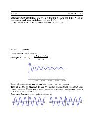
helium which is accompanied by oscillations of the
solid—liquid interface (see Ref. [1] and references
therein). A first approach to modeling this kind of
phenomenon was made by Gurtin and Podio-
Guidugli [2], who developed a mechanical theory
for the evolution of a two-dimensional interface.
They obtained, for isotropic materials in the absence
of driving force for crystallization, the law of
motion: v #v"!, where v, and v are the
normal velocity, normal acceleration and curvature
of the interface respectively. This equation can be
viewed as a hyperbolic generalization of the classical
flow by mean curvature (FMC) equation (or
curve shortening equation), v", and reduces to it
when time is rescaled tPt and the limit PR is
taken.

Our approach consists in considering the hyperbolic
phase field model
u ## # u # "u,
# "#f ()#u, (1)
in a bounded region LR with Dirichlet and
Neumann boundary conditions for the temperature
field and the order parameter respectively. Here
u represents a temperature field, is an order
parameter, , and are non-negative constants,
and f () is a real odd function with a positive
maximum equal to *, a negative minimum equal
to !* and precisely three zeros in the closed
interval [!a, a] located at 0 and $a, where a is
a positive constant. System (1) is a hyperbolic version
of the classical phase field model
u # "u, "#f ()#u. (2)
For Eq. (2), it has been shown that if the temperature
field is initially equal to the melting temperature
and Dirichlet boundary conditions are
imposed on the temperature field, a plane interface
moves according to the FMC equation (see Ref. [3]
and references therein). Planar convex curves which
move according to this law remain convex and
become asymptotically circular as they shrink.
Moreover planar embedded curves become convex
without developing singularities (see Ref. [4] and
references therein).
A derivation of the hyperbolic phase field model
is sketched in Section 2. In Section 3 we study the
interface motion for Eq. (1). We present a geometric
equation of motion which may be obtained in
a particular asymptotic limit from Eq. (1) which
extends the classical FMC equation and we study
the evolution of some simply shaped interfaces
which move according to this law of motion.
A more detailed derivation of the model and of the
equation for interfacial motion, as well as a description
of the algorithm of its solution, will be presented
elsewhere [5].
2. The equations
H.G. Rotstein et al. / Journal of Crystal Growth 198/199 (1999) 1262–1266 1263
We consider a material which can be in either of
the two phases: solid or liquid and which occupies
a fixed region in space, LR, N"1, 2, 3 possessing
a smooth boundary. These two phases are assumed
to be separated by a transition zone of finite
thickness which we approximate by a sharp interface
to be defined more precisely later. If the interface
is planar, then at the interface the solid and
liquid may coexist in equilibrium at a constant
temperature ¹ , called the planar melting temperature.
We define the reduced temperature
¹"¹(x, t) to be the difference between the actual
and the planar melting temperature; i.e.,
¹(x, t):"(x, t)!¹ . For planar interfaces, positive
reduced temperatures correspond to the liquid
phase, while negative reduced temperatures correspond
to the solid phase. In the classical phase-field
model, the two phases may be characterized by
different values of an order parameter, , which is
assumed to vary continuously though the interface,
assuming the value !1 in the solid (¹(0), #1in
the liquid (¹'0), and having rapid spatial variation
normal to the interface (see Ref. [6] and
references therein). The internal energy of the system,
e(x, t), is taken to be
e(x, t):"¹(x, t)# (x, t), (3)
where l is the latent heat of melting or solidification.
The classical theory of heat conduction based on
Fourier’s law does not take into account memory
effects present in some materials and predicts that
all thermal disturbances at a given point in the
body are felt immediately throughout the whole
body. A theory of heat conduction with finite wave
speeds for isotropic materials, has been developed,
which when linearized, yields the following expression
for the heat flux [7]
q"! A (s)e¹(t!s)ds, (4)
where the kernel or “heat relaxation function” A (s)
has been assumed to be a differentiable scalarvalued
function on (0,R) such that A (R)"0. We
shall limit our considerations here to exponentially
decreasing kernels A (t)"e where and are
non-negative constants. A review of finite and infinite
wave propagation is given in Ref. [8]. When no
heat is supplied to the body by external sources,

1264 H.G. Rotstein et al. / Journal of Crystal Growth 198/199 (1999) 1262–1266
the internal energy e"e(x, t) and the flux are related
by
eR "!div q. (5)
Combining Eqs. (3), (5) and (4) yields [9,10]
¹ # "K A (t!t)¹(t)dt. (6)
The free energy, F , of the system is assumed to
be of the form
F ()"
2 ()#F()
!S ¹ dx, (7)
where is a correlation length [6]. The term involving
the gradient is assumed to arise as a consequence
of long range interactions, the function F()
is a double-well potential (the free energy density at
zero temperature of spatially homogeneous systems),
is a positive constant, S is an entropy
coefficient [11]. The term S ¹ represents temperature
times relative entropy. The functional
derivative of Eq. (7); i.e., F /(x)"!#
F()/!S ¹, may be considered as a generalized
force indicative of the tendency of the free energy to
decay towards a minimum. We assume here that
(x) decreases with a time averaged (rather than
immediate) response to this generalized force:
" A (t!t) #
F()
#S ¹ (t)dt. (8)
Here A may be considered as a generalized force
relaxation function with characteristics similar to
A . Eqs. (6) and (8) will be henceforth called the
phase-field equations with memory. Note that
when A (t)"A (t)"(t), they reduce to the classical
phase field equations [6]. By putting Eqs. (6)
and (8) in dimensionless form, taking exponentially
decreasing kernels, differentiating with respect to t,
and rearranging terms we obtain Eq. (1), where
f () states for the dimensionless form of F()
(see Ref. [5] for details), under the scaling assumptions:
"O(), "O(), "O() and "O().
Let us note that another scaling "O(),
"O(), "O() and "O() has also been
considered [12]. Under appropriate assumptions
on the kernel, this latter scaling provides a
more general law for phase boundary motion,
v" a(t!)()d. There the kernels were assumed
to have an effective time scale for memory
of O() which also corresponds to the assumed
effective (dimensionless) thickness of the interface.
3. Interface motion
By formal asymptotic analysis of Eq. (1) taking
1, we obtained that the interface, defined as
(t; ):"x3 : (x, t; )"0 and treated as
a moving internal layer of width O(), evolves according
to the geometric law
v #v(1!v)!(1!v)"0, (9)
where denotes . Here v is the velocity in the
normal direction to the interface, and is its curvature.
We focused on the dynamics of a fully developed
layer and not on the process by which it
was generated. A general investigation of the interface
motion governed by Eq. (9) is beyond the
scope of the present paper. Here we will consider
some simple particular cases.
For a circular interface with radius R (t), Eq. (9)
may be written as [13]
1
R "! #R
R
(1!R ). (10)
For "0, if R (0)"f '0 and R (0)"0, then
R (t)"f cos(t/f ). Thus circles shrink to points at
time t where t "f /2, and R (1 for
0(t(t . For '0, if R remains in the interval
[!1, 0], then R (t)(0 for t3(0, t ), where t is the
extinction time which we define to be such that
R (t )"0 and R (t)'0 for all t(t . A phase plane
analysis shows that for *0 circles shrink to
points for all initial conditions such that
!1(R (1 and curves starting in this region
remain within it up to extinction time. The effect of
positive is to delay the extinction time [13].
The evolution of a perturbed circle has been
studied numerically. As an illustration, the result of
numerical calculations for a perturbed circle with

H.G. Rotstein et al. / Journal of Crystal Growth 198/199 (1999) 1262–1266 1265
Fig. 1. Shrinkage of a perturbed circle for R(0)"1#0.1 sin(2), R (0)"!0.1. (a) "0 and t"0, 0.7, 1.2, 1.4. (b) "5 and t"0, 1.55,
2.52, 2.95.
initial shape and velocity given by R(0)"
1#0.1 cos(2) and R (0)"!0.1 respectively and
where equals 0 or 5 are shown in Fig. 1. For "0
we see that the interface rotates as it shrinks. This
phenomenon is almost not observable for "5.
The evolution of planar interfaces is described by
the equation
S #S (1!S )"0, (11)
where y"S (t) represents the distance between the
interface and the x-axis. Taking S (0)"f and
S (0)"g , the solution of Eq. (11) for '0 is
given by
S (t)"f $ ln(g #)$tG ln(g
#g#(1!g)e), (12)
where the upper choice of signs correspond to
g '0 and the lower choice of signs correspond to
g (0. Note that the direction of propagation de-
pends on the sign of g and as tPR the interface
will cease to move and asymptotically approach the
value f $(1/) ln(g#). When there is no
damping ("0), the solution of Eq. (11) is given by
S (t)"f #g t. A perturbation analysis of planar
interfaces on finite intervals with Neumann boundary
conditions indicates that if "0, then nonconstant
perturbations oscillate indefinitely, whereas
if '0 initial perturbations are damped though
oscillations may or may not occur depending on
the initial perturbation and the value of .
There also exist non-planar front solutions to
Eq. (9) which propagate with constant velocity v;
i.e., S(x, t)"SM (x)#vt, where SM (x) can be shown to
satisfy
(1!v)SM !v(1#SM !v)"0. (13)
The solution of Eq. (13) is given by
SM (x)" 1
2a ln[1#tan(abx#c )]#c , (14)
where a"v/(1!v), b"(1!v) and c and
c are integration constants which depend on the
initial conditions. This solution corresponds to
a “finger” of width /ab whose orientation depends
on the sign of v.
4. Conclusions and discussion
We have presented a hyperbolic extension of the
classical phase-field equations and analyzed the
special case given in Eq. (1). In this particular scaling
we have demonstrated that the evolution of
interfaces is governed by Eq. (9), a hyperbolic extension
of the classical FMC equation.
Let us note that Eq. (1) is also relevant for other
physical processes like propagation of kinks in
Josephson junctions, magnetics, etc. [13]. In particular,
for "0, the Cartesian version of Eq. (9) is
known as the Born—Infeld equation. The geometric
description of the evolution of interfaces has the

1266 H.G. Rotstein et al. / Journal of Crystal Growth 198/199 (1999) 1262–1266
advantage that it permitted us to develop and use
a crystalline algorithm to study the motion of
curves by constructing facetted approximations to
them. This algorithm which requires less calculations
than classical methods of solving PDEs is
described elsewhere [14].
References
[1] A.Y. Keshishev, A.Y. Parshin, A.V. Babkin, Sov. Phys.
JETP 30 (1990) 56.
[2] M.E. Gurtin, P. Podio-Guidugli, SIAM J. Math. Anal. 22
(1991) 575.
[3] G. Caginalp, Rocky Mountain J. Math. 21 (1991) 603.
[4] M.A. Grayson, J. Differential Geom. 26 (1987) 285.
[5] H.G. Rotstein, A.A. Nepomnyashchy, A. Novick-Cohen,
1998, preprint.
[6] G. Caginalp, Arch. Rat. Mech. Anal. 92 (1986) 205.
[7] M.E. Gurtin, A.C. Pipkin, Arch. Rat. Mech. Anal. 31 (1968)
113.
[8] D.D. Joseph, L. Preziosi, Rev. Mod. Phys. 61 (1989) 41.
[9] A. Novick-Cohen, in: Curvature Flows and Related
Topics, GAKUTO Math. Sci. Appl., vol. 5, 1995, pp.
179—198.
[10] S. Aizicovici, V. Barbu, NoDea 3 (1996) 1.
[11] G. Caginalp, P.C. Fife, SIAM J. Appl. Math. 48 (1998) 506.
[12] A. Novick-Cohen, in preparation.
[13] H.G. Rotstein, A.A. Nepomnyashchy, 1998, preprint.
[14] H.G. Rotstein, S. Brandon, A. Novick-Cohen, J. Crystal
Growth 198/199 (1999) 1256.