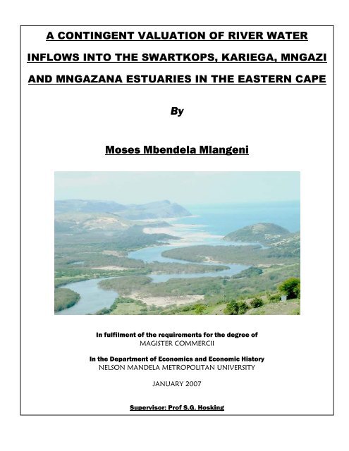
By Moses Mbendela Mlangeni - Nelson Mandela Metropolitan ...

A CONTINGENT VALUATION OF RIVER WATER
INFLOWS INTO THE SWARTKOPS, KARIEGA, MNGAZI
AND MNGAZANA ESTUARIES IN THE EASTERN CAPE
By
Moses Mbendela Mlangeni
In fulfilment of the requirements for the degree of
MAGISTER COMMERCII
In the Department of Economics and Economic History
NELSON MANDELA METROPOLITAN UNIVERSITY
JANUARY 2007
Supervisor: Prof S.G. Hosking

ABBREVIATIONS
CERM Consortium for Estuary Research and Management
CV Contingent Valuation
CVM Contingent Valuation Method
DEAT Department of Environmental Affairs and Tourism
DWAF Department of Water Affairs and Forestry
EC Eastern Cape
Ha Hectares
HPM Hedonic Pricing Method
IDZ Industrial Development Zone
INR Institute for Natural Resources
KZN KwaZulu-Natal
MAR Mean Annual Runoff
MCM Marine and Coast Management
NMMM Nelson Mandela Metropolitan Municipality
NMMU Nelson Mandela Metropolitan University
OLS Ordinary Least Squares
SA South Africa
SP Stated Preference
TWTP Total Willingness to Pay
WC Western Cape
WTA Willingness to Accept
WTP Willingness to Pay
WTW Water Treatment Works
WRC Water Research Commission
ii

ACKNOWLEDGEMENTS
My sincere gratitude goes out to the following people who have contributed to
making this study successful. I would like to thank the Economics Department
at NMMU, in particular Prof SG Hosking, for introducing me to natural resource
economics and guiding me through my research studies. I also thank Prof
Wooldridge of the Zoology Department for his valuable advice and guidance.
This research was made exciting through collaborating with several colleagues
including Dr M Du Preez, Mr G Dimopolous, Mr C-H Lin, Mr M Sale, Ms D
Erasmus, Prof J Adams, Ms A Rajkaran, Ms N Ngesi, Ms N Twala (NMMU); Mr
S Mullins, Mr G Daniels, Mr T Geldenhuys, Mr P De Wet (DWAF); Dr GR
Backenberg, Dr SA Mitchell (WRC); Dr J Turpie (University of Cape Town); Mr T
Crowley (NMMM); Ms E McNulty (Kenton-on-sea Tourism office) and Mr R Ball
(Albany Coast Water Board).
I greatly appreciate the contribution made by all participants (residents, visitors
and businesses) interviewed during the survey of the Swartkops, Kariega,
Mngazi and Mngazana estuaries. I also thank all my family and friends, for their
encouragement and support during the challenging years of this study. The
funding of the project by the Water Research Commission is gratefully
acknowledged. With the Psalm of King David Below I thank the Almighty Lord
for His amazing creation and for providing us with water to drink and air to
breathe.
Psalm 104 (excerpt)
“….The waters stood above the mountains. At your rebuke they fled
At the voice of Your thunder they hastened away.
They went up over the mountains; They went down into the valleys
To the place which You founded for them. You have set a boundary that they may not
pass over
That they may not return to cover the earth…”
iii

EXECUTIVE SUMMARY
Many South African estuaries are currently believed to be generating lower
levels of services than they used to in the past due to substantially reduced
inflow of river water, among other reasons. The basis by which river water is
allocated in South Africa has had to be re-examined. Local authorities are now
required to integrate into their development planning sensitivity to the ways
estuaries work; the relevant legislation being the Municipal Systems Act No. 32
of 2000. Sound water resource management requires that the benefits and costs of
different water allocations be compared and an optimum determined.
The Contingent Valuation Method (CVM) is used in this study to estimate the
benefits of changing allocations of river water into estuaries. This study builds on
a CVM pilot project done at the Keurbooms Estuary in the Southern Cape in year
2000 (Du Preez, 2002). Further CVM studies were conducted at the Knysna,
Groot Brak and Klein Brak estuaries (Dimopolous, 2004).
The CVM is a valuation technique based on answers given to carefully
formulated questions on what people are willing to pay for specified changes of
freshwater inflows into estuaries. The CVM depends on there being a close
correspondence between expressed answers given to hypothetical questions and
voluntary exchanges in competitive markets that would be entered into if money
did actually change hands. The fact that it has proved very difficult to establish
this correspondence has led to CVM being subject to criticism. However, many
aspects of this criticism have been addressed in the form of methods to reduce
biases, and the application of the technique has grown steadily in popularity
during the past 25 years.
iv

Four estuaries, the Swartkops, Kariega, Mngazi and Mngazana, were surveyed as
part of this study in order to determine users’ willingness to pay (WTP) for
changes in freshwater inflows. Considerable research time was devoted at the
estuaries getting to know how things worked around and in the estuaries. The
Swartkops estuary is a permanently open system within the Nelson Mandela Bay
metropolitan area. The estuary has the third largest salt marsh in South Africa. Its
banks are highly developed with residential and industrial property and it is
heavily used for both recreation and subsistence fishing by locals. The Kariega
estuary is located near the semi-rural town of Kenton-on-sea, between Port
Elizabeth and East London. Although it is permanently open, the Kariega estuary
has very low inflows of river water. It is mainly used by retired pensioners living
in holiday houses at Kenton-on-sea. The Kariega is not heavily used for
recreation and subsistence fishing, except during holidays and the festive season
because of its proximity to other estuaries such as the Bushmans and the
Kleinemond.
The Mngazi and the Mngazana estuaries are located in the Wild Coast area of the
Eastern Cape, in the Port St Johns Municipal district. The Mngazi is a temporarily
open/closed system which does not have high botanical ratings, although it is
heavily used by visitors to the well known Mngazi River Bungalows, a highly
rated hotel near the mouth of the Mngazi River. The Mngazana estuary is a
permanently open system renowned for its Mangrove forests and excellent
fishing spots. Both the Mngazi and Mngazana estuaries are located in rural areas
and are heavily used by local village residents for subsistence purposes.
The respective Total Willingness To Pay (TWTP) amounts of the four estuaries
are shown in descending order by value in Table 1. The TWTP is divided by the
proposed quantity of freshwater inflow change to obtain a unit price for the
water in Rands per m³ (see Table 2).
v

Table 1: Estimated TWTP per estuary
Estuary Predicted median Estimated no. of TWTP
WTP per annum* users annually
Swartkops (-) R244 10 000 R2 440 000
Kariega (+) R211 2 000 R422 000
Mngazana (-) R75 2 500 R187 500
Mngazi (-) R25 7 000 R175 000
Notes: * The values relate to the period from February 2003 to November 2004
** Signs after estuary names indicate specified increase (+) or decrease (-) in water inflow
It can be seen in Table 1 above that the Swartkops estuary had the highest TWTP
of the four estuaries surveyed (R2,4 million), and the Mngazi estuary had the
lowest TWTP (R175 000). The per m³ value of water flowing into each of the four
estuaries is shown in descending order in Table 2 below.
Table 2: Value of water per m³ - select estuaries in South Africa
Estuary TWTP per Change in inflow Value/ m³
annum
(millions of m³ p.a)
Swartkops R2 440 000 13,5 R0,18
Kariega R422 000 7,4 R0,06
Mngazana R187 500 10,62 R0,02
Mngazi R175 000 14,14 R0,01
Notes: Values relate to the period from February 2003 to November 2005
The contingent valuations shown in Table 2 reflect a wide range of values in
Rands per m³. As would be expected, estuaries nearer large urban populations
attract large numbers of visitors, resulting in higher WTP bids for freshwater
inflows, whereas estuaries in rural areas are not as heavily visited and many of
those who do use them are low income earning villagers.
Key words and phrases: estuary, freshwater, fish, contingent valuation,
recreation, subsistence, willingness-to-pay, conservation, permanently open,
temporarily closed.
vi

CONTENTS
Abbreviations……………………………………………………………………………ii
Acknowledgements……………………………………………………………….……iii
Executive Summary………………………………………………………………….…iv
Contents……………………………………………………………………………….…v
List of Tables………………………………………………………………………...…viii
List of Figures……………………………………………………………………….….xv
List of Appendices……………………………………………………………………xvii
CHAPTER 1: SOUTH AFRICAN ESTUARIES
1.1 Introduction ……………………………………………...……………..1
1.2 The influence of climate on estuaries………………………………..3
1.3 Classification of estuaries……………………………………………..3
1.3.1 Permanently open estuaries………………………………..…………..4
1.3.2 Temporarily open/closed estuaries………………………..………….4
1.3.3 Estuarine bays/lagoons………………………………………..……….5
1.3.4 River mouth estuaries………………………………………….……….5
1.3.5 Estuarine lakes………………………………………………..………….5
1.4 Other factors that affect the shaping of estuaries…………...…….6
1.4.1 Mouth closure and artificial breaching………………………...…….6
1.4.2 Sedimentation…………………………………………………………..7
1.4.3 Pollution and encroachment………………………………………….7
1.5 Uses of estuaries……………………………………….………………..7
1.6 Estuarine plants…………………………………………….………….9
1.6.1 Small algae (microalgae)……………………………….…………….. 9
1.6.2 Large algae (macroalgae) …………………………………….……….9
1.6.3 Submerged large plants (macrophytes) ………………...………….10
1.6.4 Salt marshes ………………………………………………..…………10
1.6.5 Reeds and sedges ………………………………………….…………10
vii

1.6.6 Mangroves …………………………………………………………….11
1.7 Estuarine animals………………………………………...…………..11
1.8 Human uses of estuaries……………………………...……………..12
1.9 Passive users of estuaries……………………………………..…….14
1.10 Predicted impacts of freshwater deprivation to estuaries …..….14
1.11 Conservation and management of South African estuaries…....16
1.12 Conclusion…………………………………………………………….17
CHAPTER 2: VALUING ESTUARIES USING THE CVM……………..……….18
2.1 The market for estuary services and deducing WTP ……...…..…19
2.2 The Contingent Valuation Method………………………...……….22
2.2.1 Theoretical foundations for application to environmental goods
....................................................................................................................22
2.2.2 The CVM gains acceptance……………………………………………22
2.3 The stages in applying the CVM……………………………....……24
2.3.1 Step 1: Establishing a credible / realistic market..............................24
2.3.1.1 Questionnaire design ……………………………………….…………24
2.3.1.2 The valuation scenario………………………………………….……..24
2.3.1.3 The payment vehicle ………………………………………….……….25
2.3.1.4 Respondent characteristics……………………………………...…… 25
2.3.2 Step 2: Administering the survey……………………………………25
2.3.2.1 Different approaches ………………………………………….………25
2.3.2.2 Elicitation methods ……………………………………………..……. 26
a. Open-ended elicitation …………………………….……………… 26
b. Single-bounded dichotomous choice (referendum method)…...27
c. Double-bounded dichotomous choice ……………………...…… 27
d. Bidding Game ……………………………………………………….28
e. Payment card………………………………………………...………28
2.3.2.3 User population and sample size determination…………………...28
viii

2.3.3 Step 3: Calculating average bids …………………………...………..31
2.3.4 Step 4: Estimating a bid function …………………………………….32
2.3.5 Step 5: Aggregating data and identifying biases …………….……..32
2.3.5.1 Incentives to misrepresent responses ………………………….…….33
2.3.5.2 Implied value cues …………………………………………………….33
2.3.5.3 Bias due to scenario misspecification ………………………………..34
2.3.5.4 Payment vehicle biases ………………………………………….…….34
2.3.5.5. Sample design and inference biases ………………………...………34
2.3.5.6 Other forms of bias ………………………………………...…………35
2.3.6 Step 6: Assessments for reliability and viability …………….…….36
2.3.6.1 Reliability of data and results ……………………………………….36
2.3.6.2 Validity of data and results ………………………………………….36
2.4 Conclusion ………………………………………………….….……....37
CHAPTER 3: THE SWARTKOPS ESTUARY ……………………………..………39
3.1 Background ……………………………………………………..……..39
3.2 Water supply sources in the NMMM ………………………...…….40
3.3 Description of the Swartkops estuary ……………………...………41
3.3.1 Physical description ……………………………………………...……42
3.3.2 Permanent residents ……………………………………………..……45
3.3.3 Uses of the Swartkops estuary ……………………………….………47
3.3.3.1 Recreational uses …………………………………………...…………47
3.3.3.2 Subsistence uses ………………………………………………….……51
3.3.3.3 Commercial and industrial uses ………………………………..……54
3.4 Identifying the target population of Swartkops estuary users….55
3.5 Setting scenarios of changes in estuary freshwater inflows….…56
3.6 Conclusion…………………………………………...…………………58
ix

CHAPTER 4: THE KARIEGA ESTUARY …………………………………………59
4.1 Physical description of the Kariega estuary ………………...…….59
4.2 Permanent residents ………………………………………………….61
4.3 Water demand in the Ndlambe municipal area …………………..64
4.3.1 Domestic use ………………………………………………………...…64
4.3.2 Commercial use ……………………………………………..…………64
4.3.3 Agricultural use ……………………………………………….……….64
4.4 Water supply sources in the Ndlambe Municipality …….………64
4.5 Uses of the Kariega estuary ……………………………….…………66
4.5.1 Recreational uses ………………………………………………………67
4.5.2 Subsistence uses ………………………………………………….……68
4.5.3 Commercial and industrial uses ……………………………..………69
4.5.4 Agricultural uses ………………………………...…………………….70
4.6 Identifying the target population of Kariega estuary users ….…70
4.7 Setting scenarios of changes of estuary freshwater inflows ……72
4.8 Conclusion …………………………………………………………..…73
CHAPTER 5: THE MNGAZI ESTUARY ………………………………..…………74
5.1 Physical description of the Mngazi estuary …………………….…75
5.2 Permanent residents ………………………………………….………76
5.3 Water demand in the OR Tambo district municipality ….………77
5.3.1 Domestic use ………………………………………………...…………77
5.3.2 Commercial use ………………………………………………..………77
5.3.3 Agricultural use …………………………………………..……………78
5.4 Water supply sources in the OR Tambo district municipality …78
5.5 Uses of the Mngazi estuary ……………………………….…………80
5.5.1 Recreational uses ………………………………………………………80
5.5.2 Subsistence uses …………………………………………….…………83
5.5.3 Commercial or Industrial uses ………………..………………...……86
x

5.6 Identifying the target population of Mngazi estuary users …….87
5.7 Setting scenarios of changes of estuary freshwater inflows ……...90
5.8 Conclusion …………………………………………………………….90
CHAPTER 6: THE MNGAZANA ESTUARY ……………………………………..92
6.1 Physical description of the Mngazana estuary ……………………92
6.2 Permanent residents ………………………………………….………96
6.3 Water demand around the Mngazana estuary ……………………97
6.3.1 Domestic use …………………………………………………...………97
6.3.2 Commercial use …………………………………………………..……97
6.3.3 Agricultural use ………………………………………………..………97
6.4 Uses of the Mngazana estuary………………………….……………97
6.4.1 Recreational uses …………………………………………..………….98
6.4.2 Subsistence uses …………………………………………...………..…99
6.4.3 Commercial uses ……………………………………………..………101
6.5 Identifying the target population of Mngazi estuary users.....…101
6.6 Setting scenarios of changes of freshwater inflows ……….……102
6.7 Conclusion ……………………………………………………………103
CHAPTER 7: ANALYSIS OF RESPONSES ………………………………..……104
7.1 Introduction …………………………………………………….……104
7.2 Descriptive Statistics …………………………………………..……104
7.2.1 Sample information …………………………………….……………104
7.2.2 Socio-economic characteristic profiles ……….……………………106
7.2.3 Knowledge of estuary ecology …………………………….………108
7.2.4 Importance attached to various activities …………………………109
7.2.5 Frequency of use ……………………………………..………………114
7.2.6 WTP for water inflow into estuaries …………………….…………115
xi

7.2.7 Conclusion……………………………………………….……………116
CHAPTER 8: THE FITTING OF WTP FUNCTIONS ……………………..……118
8.1 Introduction………...… …………………………………………..…118
8.2 Coefficient expectations ………………….………….………..……119
8.3 The Swartkops estuary bid curves ……….………..…..…….……121
8.3.1 Tobit models (complete and reduced).…………………………..…121
8.3.2 Results and interpretation …………………………………………..123
8.4 The Kariega estuary bid curves ………………………..………….123
8.4.1 Tobit models (complete and reduced) …………………………..…123
8.4.2 Results and interpretation ……………………………………..……125
8.5 The Mngazi estuary bid curves ………………………..…………..125
8.5.1 Tobit models (complete and reduced) ………………………..……126
8.5.2 Results and interpretation ……………………………………..……127
8.6 The Mngazana estuary bid curves…………………..…………….127
8.6.1 Tobit models (complete and reduced) ………………………..……128
8.6.2 Results and interpretation ……………………………………..……129
8.7 Predicted WTP ……………………………..………………………..129
8.8. An assessment of the credibility of the results ………….………130
8.8.1 Validity …………………………………………………………..……130
8.8.2 Reliability (repeatability) issue …………………………..…………132
8.9 Conclusion ……………..……………………………………….……132
CHAPTER 9: CONCLUSION AND RECOMMENDATIONS ..........................134
9.1 Expected findings ……………………………….….………………136
9.1.1 Sensitivity of estuary to water reductions …………………………136
9.1.2 Direction of specified change of water inflow………………...…...136
9.1.3 Size of user population……………………………………………….137
9.2 Confidence in results ……………………………………….………137
xii

9.3 Conclusion on the appropriateness of applying the CVM to value
freshwater inflow into estuaries ………………......………………137
9.4 Conclusion on the administration of the surveys ……….………138
9.5 Recommendations ………………………………………...…………138
9.5.1 Research perspective………………………………….….…..………138
9.5.2 Management perspective……………………….……………………138
9.6 Some recommendations by estuary users ………………..………140
References …………………………………………………………………….………144
Appendices ………………………………………………………………..…….……160
References to Appendices…………………………………………………....……..194
LIST OF TABLES
xiii

Table No. Title Page No.
1 Estimated TWTP per estuary vi
2 Value of water per m³ - select estuaries in South Africa vi
1.1 Selected animals and plants found in South African estuaries 8
1.2 Estuary users 13
3.1 Eastern Cape water supply - Western Region district 40
3.2 Water sources and dams supplying the NMMM area 41
3.3 Swartkops estuary fishing and boating clubs 48
3.4 Once-a-month count of boats at the Swartkops estuary in 2003 49
3.5 Authorised quantities of bait harvests at the Swartkops estuary 51
3.6 Once-a-month count of people at the Swartkops estuary in 2003 55
3.7 Estimated total population of the Swartkops estuary users 55
3.8 Monthly flow volumes of the Swartkops River (million m³) 57
4.1 Kenton-on-Sea total population 62
4.2 Alternative Kariega/Bushmans water supply costs (1989 costs) 66
4.3 Households using the Kariega estuary per annum 70
4.4 Kariega estuary users’ interest in services 71
4.5 Monthly flow volumes of the Kariega River (million m³) 73
5.1 Mngazi River Bungalows staff members 86
5.2 Estimated number of households using the Mngazi estuary per
year 87
5.3 Mngazi River Bungalows visitors in 2003/2002 by province or
country of origin 89
6.1 Some of the common East Coast estuary life 95
6.2 Per Capita income earned per annum in Port St Johns 96
6.3 Local selling prices of the Mngazana estuary fish 100
6.4 Other Mngazana estuary harvests for subsistence purposes 100
6.5 Estimated household users of the Mngazana estuary per year 102
xiv

7.1 Number of questionnaires completed and valid responses 105
7.2 Category of user/respondent 105
7.3 Socio-economic profile of respondents 106
7.4 Relationship between education level and knowledge of estuary
ecology 108
7.5 Percentage of respondents by WTP amount 115
8.1 Description of selected variables in the multiple regression analysis 120
8.2 The Swartkops estuary bid curve estimate – complete model 121
8.3 The Swartkops estuary predictive model (a reduced model) 122
8.4 The Kariega estuary - bid curve estimate (complete model) 124
8.5 The Kariega estuary predictive model (reduced model) 124
8.6 The Mngazi estuary - bid curve estimate (complete model) 126
8.7 The Mngazi estuary predictive model (reduced model) 126
8.8 The Mngazana estuary - bid curve estimate (complete model) 128
8.9 The Mngazana estuary predictive model (reduced model) 128
8.10 Predicted mean and median WTP 130
8.11 Sample validity rating 131
9.1 TWTP – select estuaries in South Africa 135
9.2 Value of water per m³ - select estuaries in South Africa 135
9.3 Swartkops estuary users’ comments /recommendations 140
9.4 Kariega estuary users’ comments /recommendations 141
9.5 Mngazi estuary users’ comments and recommendations 142
9.6 Mngazana estuary users’ comments and recommendations 143
xv

LIST OF FIGURES
Figure No. Title Page No.
1.1 The Mzimvubu River Mouth estuary at Port St Johns. 1
1.2 Common birds found in estuaries 8
3.1 The Swarkops estuary near the Nelson Mandela Bay 41
3.2 Street map of residential areas near the Swartkops estuary 46
3.3 A bait digger holds a pump and permit at Swartkops estuary 52
4.1 The Kariega estuary at Kenton-on-sea. 59
4.2 Street Map of Kenton-on-sea 63
5.1 The Mngazi and Mngazana River catchments 74
5.2 The Mngazi River Bungalows on the banks of the estuary 77
5.3 The Port St Johns Water Supply Scheme 79
5.4 A Kingfisher on a water-level stick in the Mngazi estuary 82
5.5 Village girls selling craftwork at Mngazi River Bungalows 85
6.1 The Mngazana estuary in Port St Johns 92
7.1 Category of User/Respondent 107
7.2 Respondents’ race – all four estuaries 107
7.3 Respondents’ gender 107
7.4 Line plot for correlation between education level and knowledge of
estuary ecology 109
7.5 Relative importance attached to boat sports (excl. fishing) 110
7.6 Relative importance attached to swimming 110
7.7 Relative importance attached to fishing 111
7.8 Relative importance attached to viewing estuary 111
7.9 Relative importance attached to estuary proximity 112
7.10 Relative importance attached to bird watching 112
7.11 Relative importance attached to commercial activities around
estuary 113
xvi

7.12 Relative importance attached to preservation of unique estuary
xvii
features 113
7.13 Average use of estuary services per year 114
7.14 Number of members per household using estuary services 115

LIST OF APPENDICES
No. Title Page No.
xviii
1 Characterisation of South African estuaries 160
2 Standard questionnaire used in the estuaries survey 166
3 Field experiences – Swartkops estuary CVM survey 172
4 Some common birds found in the Swartkops river catchment 174
5 Some common fish found in the Swartkops estuary 175
6 Field experiences - Kariega estuary CVM survey 176
7 Some common birds found in the Kariega estuary catchment 177
8 Some common fish found in the Kariega estuary 178
9 Field experiences – Mngazi estuary CVM survey 179
10 Some common fish found in the Mngazi estuary 181
11 Field experiences – Mngazana estuary CVM survey 182
12 Some common fish found in the Mngazana estuary 184
13 Trees of the Mngazi and Mngazana river forests 185
14 Common birds in the Mngazi/Mngazana River Catchment 186
15 Example of monthly fishing permit 187
16 Example of annual fishing permit 189
17 Information brochure handed out during CVM survey 191
18 Additional comments by Mngazana estuary users 192

CHAPTER 1:
SOUTH AFRICAN ESTUARIES
1.1 Introduction
South Africa (SA) has a coastline of about 3 000 kilometres (Baird, 2002: 37),
stretching from KwaZulu-Natal (KZN) to the Western Cape (WC). Along this
coastline there are about 250 – 260 places where rivers from inland join the sea,
forming what are known as estuaries (Whitfield, 2000). The National Water Act
(1998) defines an estuary as a partially or fully enclosed body of water that is
open to the sea, permanently or periodically and, within which the seawater is
diluted to an extent that is measurable, with freshwater drained from inland.
Figure 1.1 below shows an example, the Mzimvubu river mouth estuary (which
is found in the same district as the Mngazi and the Mngazana estuaries).
Figure 1.1: The Mzimvubu River Mouth estuary at Port St Johns.
Source: Bate et al, 2003.
Along the SA coastline there are a large number of estuaries - 258 according to
some scientists (Whitfield, 2000).
1

The focus of attention in this study was to value freshwater allocations to four
Eastern Cape (EC) estuaries – the Swartkops, Kariega, Mngazi and Mngazana.
The Swartkops estuary is a permanently open system within the Nelson Mandela
Bay metropolitan area. The estuary has the third largest salt marsh in SA. Its
banks are highly developed with residential and industrial property and it is
used heavily for both recreation and subsistence fishing by locals. The Kariega
estuary is located near the semi-rural town of Kenton-on-sea, between Port
Elizabeth and East London. Although it is permanently open, the Kariega estuary
has had very little inflow of river water. For much of the year it is mainly used by
retired pensioners living in holiday houses at Kenton-on-sea. The Kariega is not
heavily used for recreation and subsistence fishing, except during holidays and
the festive season because of its proximity to other estuaries such as the
Bushmans and the Kleinemond.
The Mngazi and the Mngazana estuaries are located in the Port St Johns
Municipal district of the Eastern Cape, also known as the Wild Coast. The
Mngazi is a temporarily open/closed system. Although it does not have high
botanical ratings, it is regularly used by guests of the well known Mngazi River
Bungalows, a highly rated hotel near the mouth of the Mngazi River. The
Mngazana estuary is a permanently open system renowned for its Mangrove
forests and excellent fishing spots. Both the Mngazi and Mngazana estuaries are
located in rural areas and are heavily used by local village residents for
subsistence purposes.
Many estuaries in SA are generating lower levels of services than they used to in
the past due to substantially reduced inflow of river water, among other reasons
(Hosking et al, 2004). In an attempt to estimate the benefits of maintaining
allocations of river water into estuaries, this study applies the Contingent
Valuation Method (CVM) to value appropriate “public purchases” of freshwater
2

for the estuaries. The study builds on previous CVM studies conducted at the
Keurbooms/Bitou estuary (DuPreez, 2004) and at the Great Brak, Little Brak and
Knysna estuaries (Dimopolous, 2005).
This chapter describes the different types of estuaries, their fauna and flora, and
identifies some of the negative consequences of reductions in freshwater inflows
into estuaries. The size, shape and nature of SA estuaries are determined by
climate, hinterland topography, wave energy, sediment supply and different
coastal characteristics (Baird, 2002: 37).
1.3 The influence of climate on estuaries
The SA coastline can be divided into three broad climatic regions: a subtropical
region from the northern border of KZN to the Mbashe River, a warm temperate
region from the Mbashe River to Cape Point in the south and a cool temperate
region along the west coast (Baird, 2002:38).
The topography and climate of the coastal region have a huge influence on the
type of estuary that forms. Rainfall is a crucial element in determining the nature
of estuaries. The eastern coastline has steeply tilted coastal plains that receive
heavy rainfall during summer months (Baird, 2002:37). The west coast, on the
other hand, is more arid than the east coast and less tilted, and estuaries become
functional only during times of heavy rainfall (Baird, 2002:37).
1.3 Classification of estuaries
Estuaries are classified as permanently open, temporarily open/closed, estuarine
bays/lagoons, river mouths and estuarine lakes (Whitfield, 1992). A more
detailed characterisation of individual SA estuaries is provided in Appendix 1.
3

1.3.1 Permanently open estuaries
Permanently open estuaries are normally found in catchment areas that have a
perennial river and strong tidal exchange with the sea (Breen et al, 2001). When
river flow conditions are low, the tidal exchange keeps the mouth open, e.g. the
Swartkops estuary in the Nelson Mandela Bay metropolitan area. The size of the
catchment areas of such estuaries can vary between 500 km 2 and 10 000km 2
(Breen et al, 2001). Common features of permanently open estuaries include salt
marshes in temperate regions and mangrove forests in tropical areas (Breen et al,
2001). Another common feature is the eelgrass (Zostera capensis), which may be
present sub-tidally, especially in middle to lower reaches of the estuary (Breen et
al, 2001). Salinity levels usually fluctuate between 5 and 35 parts per thousand,
although hypersaline (>35 parts per thousand) conditions sometimes develop
during times of high evaporation and low or no river inflow (Breen et al, 2001).
1.3.2 Temporarily open/closed estuaries
Approximately 70% of SA estuaries are prone to temporary closures of the river
mouth (Breen et al, 2001). The reasons for this closure are many: sandbar
formation at the mouth due to drought, high levels of water consumption from
rivers and interference with the hydraulic structure of estuaries, inter alia. The
duration of the mouth closures varies from a few months to periods of a year and
longer (Breen et al, 2001). Temporarily open/closed estuaries typically have
small catchments and limited penetration by tidal waters when they are open.
The mouth usually opens during periods of high rainfall, e.g. the van Stadens
estuary.
4

1.3.3 Estuarine bays/lagoons
Estuarine lagoons, also known as estuarine bays, have continuously open
mouths due to there being a strong tidal exchange (Breen et al, 2001). A regular
replacement of marine water occurs in the lower and middle reaches of this type
of estuary, e.g. the Richards Bay and Knysna estuaries (Breen et al, 2001). The
dominant mixing process is tidal and riverwater influences only feature in the
upper areas of the estuary (Whitfield et al, 1994). The mixing process at these
estuaries is sometimes enhanced by dredging activities at the mouth, e.g. at St
Lucia and Richards Bay.
1.3.4 River mouth estuaries
When river water rather than sea water dominates the physical process, the
estuary is classified as a river mouth estuary (Breen et al, 2001). These estuaries
are usually permanently open to the sea (Breen et al, 2001). Marine water
penetration into the river is therefore confined to the lower reaches of the river,
e.g. Orange River mouth. Salinity levels tend to approach oligohaline conditions
in the middle reaches (Breen et al, 2001). Tidal inlets often remain permanently
open, although sea water penetrates only a short distance up the estuary on a
flood tide. The catchment areas of these rivers are usually large and the rivers
generally carry a high silt load (Breen et al, 2001).
1.3.5 Estuarine lakes
Estuarine lakes mostly evolved from drowned river valleys that have been
separated from the sea by vegetated sand dune systems (Breen et al., 2001). In
some cases the barrier dune has completely isolated the water body, although
5

elic estuarine biota sometimes survives. These systems are usually referred to
as coastal lakes (Breen et al, 2001). Some estuarine lakes retain their marine
connection, although the link may be temporary. Salinity values in the lake may
vary considerably, ranging from oligohaline (35 parts per thousand) depending on freshwater inflow (Breen et
al, 2001). Consequently, the biotic composition in the lake varies between
extremes and may remain at extreme levels for long periods (Breen et al, 2001).
Estuarine lakes are connected to the sea by channels of varying length and width
(Breen et al, 2001). An estuarine lake can have a mouth that is either open, e.g. the
Wilderness, or closed, e.g. the Swartvlei (Breen et al, 2001).
1.4 Other factors affecting the shaping of estuaries
1.4.1 Mouth closure and artificial breaching
When there is no or little fluvial action sand bars can form at the river mouth and
this can result in closure of the mouth. When the freshwater input resumes,
water dams up behind these sand bars (Allanson and Baird, 1999). This
damming of water often leads to the flooding of property along riverbanks
(Allanson and Baird, 1999). Artificial breaching of estuary mouths is sometimes
used to prevent the flooding problem, but this solution can also have serious
negative long-term impacts on the sediment dynamics and biota of an estuary
(Allanson and Baird, 1999:297). The sudden drop of water levels, caused by
artificial breaching, leads to large losses in invertebrate biomass (found in weed
beds) and large losses in avifauna. For example, the population of red-knobbed
coots (Fulicia cristata) declined significantly due to periodical artificial breaching
of the Bot River mouth (Allanson and Baird, 1999:297). During mouth closure
many fish species are cut off and lost to estuaries as their reproductive cycles are
disrupted due to the fish being trapped out of or within the estuary.
6

1.4.2 Sedimentation
River mouth closure may also result from sedimentation. The results of large
amounts of sediment collecting in estuaries are listed below (Allanson and Baird,
1999):
• a shallower estuary basin and possibly reduced water surface area;
• a higher water temperature affecting the survival of certain plant and fish
species and
• a collection of sand and silt, making the estuary less appealing to recreational
and commercial users.
1.4.3 Pollution and encroachment
Some estuaries have had their estuarine functions severely undermined due to
inflows of industrial, domestic and agricultural pollutants and encroachment on
the banks by housing development (Allanson and Baird, 1999:300). This
development is frequently undertaken with little sensitivity to its impact on the
terrestrial biota. In addition to the housing encroachment, the building of roads,
railways, bridges and dams all too often cut off estuarine systems from the
coastal zone and their feeder river systems (Allanson and Baird, 1999).
1.5 Uses of estuaries
Human beings, animals and plants all use estuaries in various ways. In SA
estuaries provide services for recreational and subsistence users. SA estuaries
have been estimated to be worth R153 000 per hectare (ha) annually (prices as at
year 2000) - R3 500 per ha in food production, R2 550 per ha in recreation and
7

R141 000 per ha in nutrient cycling (Lamberth, et al, 2003:1). A study by Lamberth
and Turpie (2001) estimated that the value of estuaries to the SA fishing
community was R951 million (at 1997 prices). This total was made up of the
value of the estuary fisheries (R433 million at 1997 prices) and the value of
estuary dependant fisheries in the inshore marine environment (R518 million at
1997 prices).
Table 1.1 below provides examples of some of the animals and plants found in
SA estuaries.
Table 1.1: Selected animals and plants found in South African estuaries
Prawns / bait Crabs Fish Birds Vegetation Microscopic
organisms
Other
Mud Spider Mullet Pelican Mangroves Detritus Phytoplankton
Pink Hermit Bream Fish Eagle Halophytes Bacteria Zooplankton
Pencil Rock Grunter Kingfisher Reeds Algae Bottom
Dwellers
Swimming Mudskipper Duck Sea Grasses
Carid Garrick Heron Salt marshes
Tapeworm Goby Hamerkop Zostera beds
Bloodworm Giant kob Sandpiper
Source: Bouwer, 2003.
Figure 1.2: Common birds found in South African estuaries
Heron Pelican Fish Eagle
Source: http://www.google.images
8

The biggest estuary in SA is St Lucia in KZN - an estuarine lake of 38 290 ha in
size (Wikipedia, 2005). There are also a large number of very small estuaries –
some so small in size that they are not even named and listed. Although these
very small estuaries often have important ecological functions, most are not
significant from a recreation perspective.
1.6 Estuarine plants
Plants in SA estuaries are influenced by the availability of unpolluted freshwater
inflow for survival. SA estuaries have six different plant communities (Breen
and McKenzie, 2001). These are: small algae, large algae, submerged large
plants, salt marshes, reeds and sedges and mangroves.
1.6.1 Small algae (microalgae)
Small algae are found on mud, sand and bigger plants (Breen and McKenzie,
2001). These organisms give surfaces a green or brown tinge and are a good
indicator of nutrient status and pollution. When these organisms start to die,
their decay can consume so much oxygen that fish and other organisms are also
killed (Breen and McKenzie, 2001).
1.6.2 Large algae (macroalgae)
Large algae are found in most estuaries and are made up of two main groups,
namely those with thread-like (filamentous) form and those that are firmly
attached and have a leafy (thalloid) form (Breen and McKenzie, 2001).
9

1.6.3 Submerged large plants (macrophytes)
Macrophytes are rooted plants that have stems and leaves that may reach the
water surface (Breen and McKenzie, 2001). Even though these species are able to
survive strong tidal currents, whole beds are often washed out to sea during
floods. Some species boast beautiful flowers making the estuary more attractive
to the eye (Breen and McKenzie, 2001). Submerged macrophyte beds are
important habitats for other organisms living in estuaries, e.g. fish.
1.6.4 Salt marshes
Salt marshes are areas that have a high concentration of sea salt and are
important habitats for certain invertebrates, e.g. crabs, and a source of organic
litter that sustain many species (Breen and McKenzie, 2001).
1.6.5 Reeds and sedges
Reeds and sedges in estuaries normally indicate a fresh or brak (slightly saline)
water environment (Breen and McKenzie, 2001). During droughts and times of
high salinity they often die back, but recover after floods have flushed away the
saline water. Reeds and sedge beds provide a source of energy and nutrients
during the freshwater phase of some estuaries, because they substitute those
plant species that flourish during saline conditions (Breen and McKenzie, 2001).
They also often supply subsistence users with materials for craftwork and the
construction of huts.
10

1.6.6 Mangroves
Mangroves are trees and shrubs that grow in tidal and saline coastal areas (Breen
and McKenzie, 2001). High tide causes their aerial roots and lower stems to be
submerged, but they can be exposed for several hours at low tide. They are
intolerant of continuous flooding with either fresh or saline water that cover their
roots because this restricts the exchange of gases, especially oxygen. Small
organisms are known to colonise the stems and roots of mangroves. These small
organisms, together with leaf litter, supply energy and nutrients for other
species. The wood extracted from mangroves is durable and used in building
huts and fencing (Breen and McKenzie, 2001).
1.7 Estuarine animals
SA estuaries boast a wide variety of invertebrates, fishes and birds (Breen and
McKenzie, 2001). Invertebrates are animals that do not have a backbone, e.g.
crabs and worms. Some of these invertebrates, e.g. the crown crab and sand
shrimp are known as benethic species and live on top of the sediment, while
others, e.g. bloodworm and sand prawn, live in the sediment. There are also
some invertebrates (the nektonic species) that swim actively in the water column,
e.g. the swimming prawn (Breen and McKenzie, 2001). Benethic species release
nutrients by burrowing and water pumping. These invertebrates are important
processors of living and dead plant material, making energy and nutrients
available to other species (Breen and McKenzie, 2001).
Fish can be divided into five main categories depending on their origin,
biological adaptation to estuarine conditions and their degree of dependence on
estuaries for their survival (Breen and McKenzie, 2001). The main category is the
marine species that breed at sea and whose juveniles show various degrees of
11

dependence on estuaries as nursery areas. Some of these fish feed on plant
material, such as the Stumpnose. Others, such as mullet, feed off fine living and
dead material. Grunter and cob are carnivorous, feeding on other animal
species.
A second category of fish comprises of estuarine species that breed within
estuaries and spend most of their lives within these systems (Breen and
McKenzie, 2001). A third category of fish is the freshwater species. The extent to
which they penetrate the estuary is determined by their salinity tolerance (Breen
and McKenzie, 2001). The fourth species is comprised of marine species that
stray into estuaries, but are not dependent on estuaries for their survival (Breen
and McKenzie, 2001). The fifth group is comprised of anguillid eels that use
estuaries as a conduit between the sea and river (Breen and McKenzie, 2001).
These eels swim upstream during migration and return along the same path on
their way to the marine environment, where spawning occurs.
Birds are attracted by the many different food resources and habitats provided in
estuaries. Waders, Waterfowl, Kingfishers, Cormorants, Gulls, Terns, Egrets and
Herons have all been known to inhabit estuaries. Some birds feed on estuary
vegetation, e.g. the Red-knobbed Coot. Others feed mainly on invertebrates, e.g.
the Green Shank, and still others feed on fish, e.g. the Fish Eagle and Cormorant.
1.8 Human uses of estuaries
People from all racial groups, males, females, children, youths and the elderly
use SA estuaries. The users of SA estuaries range from residents living along
estuary banks to domestic and international tourists. SA estuaries are mainly
used for recreational purposes. The recreational users, in turn, support
commercial and subsistence operations. Subsistence estuary users are common in
12

SA. Often, estuaries have unique biotic or non-biotic features that induce tourists
to visit them.
Most estuaries are open for use to the public and are accessible free of charge.
Sometimes there are clashes between users, e.g between boaters and fishermen,
or bird watchers and bait collectors. In some cases tensions have developed
between recreational users and subsistence users because the former see
estuaries as a special place for getting a peace of mind and tranquility, away
from the hustle and bustle of enterprise in urban areas, while the latter see the
former group as a potential source of livelihoods. Some recreational users of
estuary services allege that the presence of subsistence fishermen brings back the
hustle and bustle holidaymakers are attempting to escape from, thereby spoiling
the atmosphere sought by the holidaymakers. Bait collection and fishing are the
main subsistence activities. In 2002, a total of 859 subsistence fishing rights were
issued to communities in KZN and EC (DEAT, 2003). Table 1.2 below gives a
breakdown of some users of estuaries in SA.
Table 1.2: Estuary users
Recreational Commercial
(within a 10km radius of the mouth)
Subsistence
Fishermen Food and grocery stores Bait collectors
Boaters Bait and fish tackle shop Fishers
Canoes Fuel station Mussel/Oyster collectors
Swimmers Bank and Post office Tourist guides
Surfers Water sports clubs Security
Bird-watchers Hotels & Guest Houses Vehicle washers
Scene viewers Bottle stores General assistants
Beach strollers Boat rides and hire services Labourers
Picnickers Net repairs
Source: Wooldridge, 2004
Crafters
13

1.9 Passive users of estuaries
People who do not engage in actions with the intention of enjoying some service
of the estuary, but who nevertheless derive benefit from it were classed as
passive users (or non-users) in this study (Hosking et al, 2004). These users were
difficult to identify. Although their use is indirect their benefit is real and
consequently it is an integral part of the total benefit yielded by an estuary. An
example of passive use of an estuary is the enjoyment derived while passing
through an estuary in a car, bus or train, where the intention of the trip was not
to visit the estuary, but something else. The enjoyment of the estuary by this
person is a by-product of an activity that did not have the attainment of this joy
as its main purpose. In principle there are many other types of non-users other
than those identified above, but for the estuaries under consideration and aims of
this study, their omission from the analysis was deduced to be of negligible
consequence.
1.10 Predicted impacts of freshwater deprivation to estuaries
Estuaries are reliant on uninhibited access to marine and freshwater links in
order to function properly, but due to various forms of abstraction from SA’s
rivers, there is a growing deficiency of freshwater inflows to SA estuaries
(Lamberth, et al, 2003:2). These deficiencies can have adverse consequences for
estuarine habitats. The adverse consequences can take the form of reduced
wetland services.
An extreme consequence of reduced freshwater inflow into an estuary is river
mouth closure (Wooldridge, 2003). It leads to severe disruption of estuarine
functioning. The most typical consequence of freshwater inflow reduction is a
change to estuary size (Wooldridge, 2003). When the mouth of the estuary closes
14

it can result in increases in the area covered by water, but also to a build up of
contaminants in the estuary, because no flushing with the sea takes place
(Wooldridge, 2003). These changes in water quality in turn reduce the
attractiveness of the estuary to recreational users.
Several other negative changes for recreational users may also take place due to
changes in freshwater inflow. Firstly, reduced freshwater inflows undermine the
estuary as a habitat (Wooldridge, 2003). As a result there are less fish available to
be caught. These fish include catadromous species that migrate from freshwater
to the sea in order to breed, e.g. eels and freshwater mullet, and if the mouth
closes, also Spotted Grunter (Wooldridge, 2003).
Secondly, reduced freshwater inflows may reduce the yields of invertebrates
available at the estuary, e.g. bloodworm, pink prawn, mud prawn and pencil
prawn (Wooldridge, 2003). Fishermen frequently use these species as bait. By SA
law the limit for prawns harvested at estuaries is 50 per day for each type of
prawn (Wooldridge, 2003). If the mouth of an estuary closes approximately 25%
of the prawn population is lost annually, so that after four years, ceteris paribus,
the entire prawn population could be lost. In addition, increases in weed growth
reduce the area available for mud-prawn colonization (Wooldridge, 2003).
Thirdly, there may be a reduction in the area colonised by plant activity
(Wooldridge, 2003). This reduction in plant services in the estuary may lead to an
increase in turbidity, a reduction in water purification (because of less reed bed
action), a reduction in oxygen generation and a reduction in habitat and food for
birds, fish and invertebrates (Wooldridge, 2003). Fourthly, reduced freshwater
inflow in the absence of mouth closure may lead to a reduction in the estuary
size and the area available for foraging birds, for example, waders like Grey
Plovers, Curlew Sandpipers and black-winged Stilts (Wooldridge, 2003).
15

1.11 Conservation and management of SA estuaries
Freshwater inflows into SA estuaries are being undermined in various ways,
mainly by increased abstraction of river water for urban use and agriculture, and
decreased runoff into rivers due to commercial forestry and replacement of
indigenous vegetation with higher water consuming alien vegetation. In the
event of acute shortages of freshwater inflows into estuaries, new supplies can be
secured in a number of ways, of which the three most popular ones are, demand
management, removal of alien vegetation growth and supplementation schemes
in which water is imported from other river basins. In all these cases the
increased supply measures have cost implications, such as, benefits foregone by
urban and farm users or costs incurred while cutting back unwanted vegetation
or transferring water between basins.
Establishing whether future schemes to augment water supplies have a sound
economic rationale requires two tasks to be undertaken. Firstly, ecologists must
predict the adverse effects that arise upon specific reductions in water inflows,
for instance mouth closures, reductions in estuary size or deterioration in quality
habitat. Secondly, economists must apply some valuation method to estimate
society’s willingness to pay for a water supply arrangement that prevents the
predicted adverse consequences from occuring.
The conservation and management of SA estuaries rests mainly on the shoulders
of the users, the Department of Water Affairs and Forestry (DWAF) and the
Department of Environmental Affairs and Tourism (DEAT). The DEAT has a
law enforcement wing, the Marine and Coast Management (MCM) division,
which is responsible for the direct management of the estuaries themselves. Local
authorities and nature conservation authorities are responsible for land use
management around the estuaries. DWAF is responsible for allocating
16

freshwater to estuaries. Recently estuary management forums have been
established by concerned estuary users in some estuaries. Other organizations
with an interest in estuary conservation and management include the
Consortium for Estuarine Research and Management (CERM), the Institute for
Natural Resources (INR), and the Estuarine and Coastal Sciences Association.
1.12 Conclusion
There are just over 250 estuaries in SA and they have diverse natural
characteristics and productivity patterns (Whitfield, 2000). South Africans
mainly use estuaries for recreation, although there is also a significant group of
subsistence users. Estuaries are also rich habitats for many types of flora and
fauna. Some SA estuaries are currently facing problems, one of which is the
amount of freshwater being allocated to them. This dissertation aims to provide
some guidance on this issue, by generating values of estuarine services
maintained due to the public purchase of freshwater inflow allocation to selected
estuaries.
The remainder of this dissertation is organised as follows. Chapter 2 overviews
the method used in this study to value estuary services, viz. the Contingent
Valuation Method (CVM). Chapters 3, 4, 5 and 6 outline study site information of
the estuaries selected for this study, namely the Swartkops, Kariega, Mngazi and
Mngazana. The author of this dissertation placed considerable emphasis in
getting to know the relevant estuaries and their users well and spent many days
at these locations observing “how things worked” around and in the estuaries.
Chapter 7 provides an analysis of the responses from the surveys conducted at
these estuaries, Chapter 8 covers results of fitting willingness to pay functions
and Chapter 9 draws conclusions and recommendations based on the analysis.
17

CHAPTER 2:
VALUING ESTUARIES USING THE CVM
The Contingent Valuation Method (CVM) is applied in this study to determine
the worth of freshwater flowing into four estuaries in the Eastern Cape: the
Swartkops estuary in the Nelson Mandela Bay metropolitan area, the Kariega
estuary at Kenton-on-sea and the Mngazi and Mngazana estuaries in the Port St
Johns district. This chapter overviews the CVM as implemented in these
estuaries. Common biases and some tests for validity are identified and ways
some of these biases may be addressed are considered. The objective of applying
the CVM is to determine willingness-to-pay (WTP) for the goods/services in
which one is interested.
The term contingent valuation was first introduced by S.V. Ciriacy-Wantrup in
1947 (Epstein, 2002). He drew attention to various procedures that should be
followed when conducting interviews in which subjects were asked how much
money they were willing to pay for successive additional quantities of a
collective extra-market good.
CVM has since become widely applied. In developed countries it is used to value
water quality improvements, to value the benefits of reduced air pollution and to
value the existence values of wilderness areas or ecologically important species,
inter alia (Perman et al, 1996).
18

2.1 The market for estuary services and deducing WTP
Value includes both non-monetary and monetary benefits and the worth that a
user attaches to a resource, good or service (Backeberg, 2007). In contingent
valuation a monetary value which people are willing to pay is derived from the
benefit they expect to receive from a good or service (Backeberg, 2007). Since
there is no functioning market process, it is an indication of the price of the good
or service. However, it is contentious because it reflects intentions and not actual
transanctions in a competitive environment of scarce goods or services
(Backeberg, 2007).
The concepts of willingness to pay (WTP) and willingness to accept (WTA)
compensation are frequently used as criteria for measuring the benefit to the
consumer of a change in the price or quantity of a good or service. WTP refers to
the amount of money income an individual would be willing to pay to secure a
welfare improvement, or equivalently, to prevent a welfare deterioration
(Perman et al, 1996). WTA refers to the monetary compensation an individual
would require to accept a welfare deterioration, or equivalently, to forego a
welfare improvement (Perman et al, 1996).
A priori, the amount that a person would be willing to pay for freshwater inflow
into an estuary depends on many things, e.g. budgets, preferences and prices of
related goods. The social WTP for estuary services is a function of the following
variables:
Summed WTPi = f (ES, EL, POP, ECON); i = 1.........n people, where
WTPi is the willingness to pay for services of estuary either in the form of
revealed or expressed preference, ES is the availability of estuary services,
19

like boatable space and probability of catching edible fish, EL are the costs
of complementary goods, like road access to the estuary and substitute
goods like swimming beaches and hiking trails, POP is the size of the
interested user and non-user population and ECON are the economic
characteristics of the interested population, e.g. their income, wealth and
scale of investment in complementary goods like fishing rods, bird
viewing equipment, boats and preferences.
In terms of this microeconomic model, summed WTP would increase if the ES
increased or the costs of using substitute goods increased or the user population
increased or the income and wealth of estuary users increased. Conversely, it is
predicted that summed WTP would decrease if the reverse occurred.
Another economic aspect of the market for estuary services is that supply is
indivisible and demand is determined by vertical summation. Environmental
resources, such as estuaries, have the characteristics of public goods, either
partially or completely. Public goods are ones that may be used by one person
without affecting the amount available for others or their cost of use. For this
reason the estimation of the social values of estuary services requires that
information be obtained about individual and social preferences in some way,
other than with reference to market prices, such as through the political forum
(Perman et al, 1996).
Yet another important economic feature of estuary services is that they are
derived from renewable resources. The flow of services estuaries yield depends
upon many things (Hosking et al, 2004); one of them being the amount of
freshwater flowing into them (see Chapter 1). The services rendered by them
declines when this inflow drops, and if it drops below a threshold, the services
may decline precipitously (Hosking et al, 2004).
20

However, the value thereby lost is revealed in markets in limited ways because
consumption of these services is by open access. One way it is revealed is in the
differences in travel expenditures and user fees incurred by people to access the
estuary services (before and after the reduction in services). These costs may be
considered as a price of the estuary services. The method of valuation aimed at
estimating value from differences in travel cost prices is called the travel cost
method (TCM).
Another way it may be revealed is in changes to the values of property with
access to the estuary services induced by reductions in this service. The method
of valuation aimed at measuring this difference is called the hedonic pricing
method (HPM).
Neither of the above methods lends itself to the subject of this study, the
valuation of changes to freshwater inflow into estuaries because to apply them
requires pin-point timing (valuations immediately before and after the change in
estuary services) and there are lags and other disturbances affecting adjustments
in the relevant markets. It was against this background that it was decided to
apply a stated preference technique to the task of valuing the change in estuary
services induced by changes in freshwater inflow, namely CVM. When a market
for the good or service does not exist, directly or indirectly, an option by which
to determine the value users place on the good is to ask them.
One of the advantages of the CVM over the revealed preference methods
described above is that it is able to incorporate in its value passive and non-use
demand (Perman et al, 1996). The CVM evolved to value public goods,
especially those yielding services to passive users (Carson, Flores and Mitchell,
1999: 100).
21

2.2 The Contingent Valuation Method
2.2.1 Theoretical foundations for application to environmental goods
The renowned British economist Sir John Hicks (Perman et al, 1996) argued that
for the individual there were cash income equivalents for changes to their utility,
and that one could restore a person to the same level they were before a change
by means of what he termed equivalent and compensating variation. This
argument is one of the bases for the Contingent Valuation Method (CVM). For
the specific application of the CVM it is assumed that additional cash income can
completely compensate any users of estuary services for utility losses they may
suffer through reductions in these estuary services.
The CVM sets out to determine what this additional cash income is. It is well
suited to value goods that are not traded in actual markets because the additional
cash income, payment or receipt, is determined with reference to a hypothetical
scenario (Gold et al, 1996).
2.2.2 The CVM gains acceptance
Being hypothetical, CVM has attracted controversy from its very inception
(Hausman, 1981). The validity of the technique depends on there being a close
correspondence between expressed answers given to hypothetical questions
(willingness to pay) and voluntary exchanges in competitive markets that would
be entered into if money actually did change hands. The fact that it has proved
very difficult to establish this correspondence has led to CVM being subject to
criticism (Azevedo et al, 2003). There can be an upward bias to valuation results if
respondents think they will not be required to actually meet the amounts which
22

they claim they are willing to pay (Leiman, 1995). In such a case the answers
given by respondents may merely reflect strength of feeling rather than
willingness and ability to pay (Leiman, 1995).
It has also been argued that in many of the situations where the CVM is applied,
a category mistake is made of quantifying judgements as if they were preferences
(Keat, 2002). Another criticism is that respondents to a valuation study may be
far from neutral in their reactions to compensation and to claims for payment,
demanding far more in compensation for the loss of an amenity than they would
be willing to pay to ensure its preservation (Leiman, 1995).
However, many aspects of the criticisms of the CVM have been addressed – in
the form of methods to reduce biases and the incorporation of tests for
consistency, and as a result, acceptance of the technique has grown steadily
during the last 25 years (Boyle and Bergstrom, 1999). In the United States of
America, the CVM was accepted by courts as a legitimate procedure for valuing
environmental changes (State of Ohio v Dept of Interior, 1989).
The CVM is now a widely used valuation tool in economic analysis. Its chief
merits lie in its very wide applicability, its versatility and, as already stated, in
the fact that it is capable of obtaining estimates of both non-use (passive) and use
values. Recent studies have shown that where a valuation can be performed
using a variety of methods, the CVM applications stand up to critical assessment
as well as other valuation methods (Cummings, Brookshire and Schulze, [1986];
Mitchell and Carson, [1989]; Arrow et al. [1993]).
23

2.3 The stages in applying the CVM
There have been many attempts to draw up guidelines for applying the CVM.
The most well known set of guidelines are those drawn up by the Blue-Ribbon
panel in the USA (Barber et al, 1997). These guidelines relate to various steps or
stages entailed in applying CVM (Hanley and Spash, 1993).
2.3.1 Step 1: Establishing a credible / realistic market
The four key issues to be considered in establishing if a credible or realistic
market exists for valuation include questionnaire design, valuation scenario,
payment vehicle and respondent characteristics.
2.3.1.1 Questionnaire design
Designing a good questionnaire is the first step to applying the CVM. The
context of the questionnaire should be as realistic as possible in order to
encourage realistic and truthful responses (Hosking et al, 2004). Because of
limited time to conduct an interview and the potential for respondent fatigue, the
questionnaire must not be overly long.
2.3.1.2 The valuation scenario
The valuation scenario defines the good in question and the nature of the change
in the provision of that good (Arrow et al, 1993: 2). This scenario is what the
respondents will value. It should correspond with a potential future event and
not one that has already occurred (Breedlove, 1994:4). Poorly defined scenarios
will elicit confused answers.
24

2.3.1.3 The payment vehicle
The payment vehicle describes the way in which the respondent is
(hypothetically) expected to pay for the good (Arrow et al, 1993). An appropriate
payment vehicle is credible, realistic, relevant and acceptable. Payments can be of
a coercive nature, such as a national tax, local tax or compulsory user fee, or in
the form of a price increase or a voluntary donation. Respondents are often
hostile to paying more taxes, but this method of payment is also often the most
realistic (Hosking et al, 2004).
2.3.1.4 Respondent characteristics
Determining respondent characteristics is an important part of the CVM
questionnaire design. It is expected that there will be a relationship between
stated values and the characteristics of the respondent and testing for these
relationships is an important validation technique (Bateman, 2002: 85).
2.3.2 Step 2: Administering the survey
The way a survey is administered is of fundamental importance to the credibility
of the results generated by applying the CVM.
2.3.2.1 Different approaches
The CVM requires a questionnaire to be drawn up (see Appendix 2) and
administered to a sample of the user population. There are many different ways
of administering surveys, for example, by mail (although this suffers from high
non-response rate), telephone or face-to-face interviews (Hosking et al, 2004). The
25

approach selected can influence the quality of information acquired and have a
major influence on the WTP/WTA results. Telephone surveys are cost effective
but not always feasible. Face-to-face surveys are the most expensive to conduct
but they provide the most effective method of data collection in many cases,
especially where on-site sampling is required (Hosking et al, 2004). In the study
reported in this dissertation (Chapters 3-8) respondents were selected for
interviewing on-site with the aim of obtaining a representative sample.
2.3.2.2 Elicitation methods
In the questionnaire a market is simulated (set up theoretically) for a non-market
good. The WTP question aims to elicit the maximum amount the good is worth
to the respondent (Wattage, 2001:5). From this response it is possible to deduce
the consumer surplus for the good being valued and a sample average
respondent WTP for the good.
Types of questions to elicit responses
There are many types of questions that can be used to elicit responses from
respondents. The main ones are listed below.
a. Open-ended elicitation
When an open-ended format is used the respondent is not given a price to accept
or reject. Asking respondents to give a monetary valuation in response to an
open-ended question presents them with an extremely difficult task (Arrow et al,
1993). This type of elicitation involves asking respondents their maximum WTP.
There are no guiding amounts suggested to respondents. Instead respondents are
26

left to state a figure based on their feeling or opinion of the project and their
financial status. Real market situations are different – people know at what prices
the goods are typically traded at or are presented with an offer and accept or
reject.
The close-ended format is currently preferred in authoritative literature to the
open-ended one because it simplifies the decision that the respondent needs to
make and makes it correspond more closely in nature to the purchase decisions
people actually have to make (Arrow et al, 1993: 49). The type of question linked
to the close-ended format is called a dichotomous-choice question.
b. Single-bounded dichotomous choice (referendum method)
Respondents say yes or no to a single WTP amount or offer (Arrow et al, 1993).
The single WTP amount or offer must be calculated very carefully because the
resultant bid is heavily influenced by it.
c. Double-bounded dichotomous choice
Following an opening offer to the respondent a second offer is made to which
they are called upon to respond – higher if they accepted the initial offer, lower if
they rejected it (Arrow et al, 1993). Again the opening offer should be arrived at
very carefully (varied randomly) as the final WTP calculated may be heavily
influenced by it.
27

d. Bidding Game
Respondents are faced with several rounds of discreet choice questions or bids;
with the final two offers defining the maximum range the respondent is willing
to pay (Arrow et al, 1993). This process can be a very laborious and time-
consuming exercise, increasing the likelihood of respondent fatique.
e. Payment card
The payment card method presents respondents with a visual aid containing a
large number of monetary amounts and respondents themselves choose the
amount they are prepared to pay by circling the relevant range (Arrow et al,
1993). This method encounters the problem that there is no formal guiding
figure presented to respondents as in the case of open-ended elicitation.
2.3.2.3 User population and sample size determination
The need to identify the population of users and select a representative and
adequate sample of respondents from this population is common to all
applications of the CVM. In this study an identical approach was taken to all the
estuaries at which surveys were administered with respect to the determination
of the target population of users and sample size. The total number of users of
the respective estuaries per annum was deemed to include all those people with
a demand for estuary services, directly or indirectly. Identifying them proved to
be a complicated task. These people cannot be identified ex ante because they
only reveal their propensity to consume estuary services when they use them
and no records are kept of their identities (Hosking et al, 2004). Most of them are
visitors to the area and not permanent residents of the land immediately adjacent
28

to the estuary. For this reason, statistically preferred respondent selection
procedures could not be applied in the sample design process.
As an alternative to these procedures it was assumed that demand was inversely
related to distance of residence (on vacation or permanent) from the estuary, and
that at some distance, the demand for estuary services became trivial (Hosking et
al, 2004). With respect to absolute non-users (not passive and not even in the
area of the estuary) it was assumed that a demand from them would only exist if
the estuary hosted something unique.
In order to determine the target populations, visits were made to municipalities,
tourism authorities, boating clubs, water sport clubs, National Parks Boards and
any other authorities that could help in determining how many users utilised the
estuary and for what purpose they did so. In addition, Geographical Information
System (GIS) census data on the size and characteristics of the population living
within 10km of the estuary mouths was consulted.
Based on all this information, the sizes of the target population of households for
each estuary were estimated, broken down into the following predominant user
categories: anglers, boaters, bait collectors, swimmers, scenery viewers,
picnickers, commercial users, subsistence users and other users. It proved
absolutely impossible to accurately identify the individuals making up this target
population because no records of them exist. For instance most of the visitors to
the Swartkops estuary were from some other part of the Nelson Mandela Bay
metropolitan area, not immediately adjacent to the estuary.
Sample determination is one of the most crucial aspects of any empirical
research. Too small a sample size undermines the significance of the statistical
29

tests (Hair et al, 1998). In order to be acceptable a sample must be representative
of the entire target population.
As a starting point for respondent selection it was assumed that those with a
demand for the estuary services would locate themselves at some stage in a
given year within a 10km radius from the mouth of each estuary; thereby
revealing their propensity to consume estuary services.
A second decision made with respect to sample design was to set its size at 5% of
the preliminary estimated target populations. This size was the maximum that
could be surveyed with the budget available.
The sample sizes that could be afforded were smaller than was desirable. This
conclusion was based on the approach taken by Cochrane (1977) with respect to
random sampling with continuous data.
The approach uses the following formulas (Equations 2.1 and 2.2 below):
2
⎛ z s α/2 ⎞
n = ⎜ ⎟ ..............................................................................................................(2.1)
o
⎝ rY
⎠
where : no = first approximation of n
α / 2
n = sample size
z = area under the normal distribution
r = relative error (error allowance about the mean)
s = standard error
Y = sample mean
30

The approach assumes that sample sizes are normally distributed. Normal
distributions are symmetric with scores more concentrated in the middle than in
the tails. Normal distributions are described as bell shaped (Gujarati, 2003:639).
If the population sizes (N) are known, the sample size can be computed as
follows:
no
n = ...............................................................................................................(2.2)
⎛ no
⎞
1+
⎜ ⎟
⎝ N ⎠
In order to populate these formulas, the relevant mean and the standard
deviation statistics were needed. Fortunately, some were available from a pilot
study conducted on users of the Keurbooms estuary services (Du Preez, 2002).
2.3.3 Step 3: Calculating average bids
After the bids made by respondents have been recorded an analysis of the bids
must be made and the responses must be coded in the appropriate variable form.
Valid responses must be distinguished from invalid ones, e.g. protest zeros. This
distinction is made with the help of follow-up questions (Hosking et al, 2004: 40).
These questions are especially useful where there is some form of protest about
the method of payment (WTP or WTA compensation) for the good in question
(Arrow et al, 1993). Protest bids are refusals to answer a valuation question, or
zero bids when the real WTP is greater than zero (protest zeros). A similar
problem can occur with (unrealistically) high bids. Ways to minimize the number
of protest bids (Hosking et al, 2004: 40) include:
• Avoiding open-ended question formats, which are associated with high
levels of protest zeros.
31

• Asking why a zero WTP was offered. Zero responses may be genuine, but
could reflect strategic behaviour of low WTP respondents. Scenarios may
be poorly understood.
• Comparing very high bids with the uncommitted income of the
respondent (WTP can not exceed income).
• Sensitising interviewers to identify protest bids.
• Inferring the WTP of a respondent from answers to other questions.
Inferred values can be taken from the WTP statements of respondents who
have similar characteristics (e.g. income and environmental service use) to
those who protest.
• Deleting protest bidders and adjusting the sample to reflect any change in
representativity (Bateman et al, 2002:82).
2.3.4 Step 4: Estimating a bid function
Information collected using questionnaires allows for the estimation of bid
functions (Hosking et al, 2004: 40). These bid functions are estimated by relating
WTP to various characteristics of respondents. There are two main purposes of
estimating bid functions - to check if responses statistically correspond with what
would be expected and to generate a valid predictive WTP model (Hosking et al,
2004: 40).
2.3.5 Step 5: Aggregating data and identifying biases
There are many factors that may induce biases. Some of the most common ones
are described below.
32

2.3.5.1 Incentives to misrepresent responses
Compliant and strategic behaviour may lead respondents to inaccurately
represent their preferences (Breedlove, 1999:9). Compliance bias occurs when a
respondent gives answers that they feel the interviewer wants to hear (Breedlove,
1999:9). Strategic bias arises when respondents intentionally misrepresent their
preferences (Breedlove, 1999:9). They do this because they believe it will
influence the amount of the good provided.
2.3.5.2 Implied value cues
Implied value cues occur when respondents decide on a valuation based on a
“clue” as to what they believe the right answer should be (Breedlove, 1990: 10).
The clue can be the opening offer. In this case there may be a starting-point bias.
A payment card approach has the advantage of avoiding a starting-point bias.
A range bias occurs when the WTP ranges people are asked to choose between
are too wide and important detail is thereby lost (Breedlove, 1990: 10). Payment
cards try to eliminate such problems, by having a comprehensive set of options
over the critical price ranges.
Where respondents focus on benchmarks (relate the goods to other similar
goods) and value in terms of these, a relation bias may occur (Breedlove, 1990:
10). If several items are being listed, items listed first are sometimes believed to
be more valuable than items listed later. Choices made that are influenced by
how the options are listed cause position bias (Breedlove, 1990: 10).
33

2.3.5.3. Bias due to scenario misspecification
Scenario misspecification or information bias arise when the scenario is
incorrectly specified according to theoretical or policy information (theoretical
bias) or when the respondent incorrectly interprets the scenario (methodological
bias). Theoretical misspecification can be minimised with sufficient research and
interviewer training before the survey takes place. The information provided
must be clear and complete (Perman et al, 1996).
2.3.5.4 Payment vehicle biases
Differences arising in WTP solely due to the method by which the respondent is
required to make payment are known as vehicle biases (Wattage, 2001: 15).
Typical payment vehicles used are utility bills, entrance fees, taxes, user fees and
higher prices. Pilot surveys should be used to determine vehicle bias potential
and method of payment preference before the final study is undertaken (Hosking
et al, 2004: 43).
2.3.5.5. Sample design and inference biases
When sample design and benefit aggregation are not properly performed this
also causes biases (Hosking et al, 2004: 44). The sample used for the CVM survey
must represent the target population, but to determine this is difficult when the
user population changes from year to year (Hosking et al, 2004: 44). It is
important to have as large a sample as possible. If different groups making up
the population are improperly represented sample selection bias will result.
Excluding non-responses can also lead to biased results. Non-responses to
questions include: “I do not know”, refusal to respond, protest zeros, obviously
34

wrong answers and responses that are inconsistent with others given in the
questionnaire (Hosking et al, 2004: 44).
Inference biases occur when one particular CVM study is used to estimate the
value of different goods (Breedlove, 1999:12).
Temporal selection bias occurs when information from one study is used for a
different time period (Breedlove, 1999: 12).
Sequence aggregation bias occurs when data from independent studies are
aggregated over additional locations or goods (Breedlove, 1999: 12).
2.3.5.6 Other forms of bias
Period bias - Visitors, residents or businesses use the estuary in different periods
of the year. For this reason, if a survey does not extend over sufficient numbers
of periods, the sample may not be representative. This sample design problem is
said to induce a period bias. Estuaries are used all year round, be it during
holidays, weekdays, weekends, month-ends and year-ends, but in order to
capture visitors the sample period must include as many of these periods as
possible. Another distinguishing feature of period bias is time of day for using
estuary. Different users use the estuary in mornings, afternoons and evenings.
The weather condition during the survey can also lead to a period bias as hot
sunny days attract swimmers, while on cold or rainy days mostly fishers may be
found in estuaries. Finally, a neap tide and a spring tide may have different
impacts on estuary usage. A lot of fishers and bait collectors use the estuary
during a spring tide.
35

Avidity bias – Avid users of a resource refers to users who use the resource very
frequently. A bias can arise if a researcher only targets such users as this could
exclude less regular (but nevertheless important) users.
2.3.6 Step 6: Assessments for reliability and validity
The credibility of a stated preference survey is assessed through tests of the
reliability and validity of data and results.
2.3.6.1 Reliability of data and results
Reliability refers to the degree of replicability of a measurement or low variation
between results of different samples of the same population (Bateman et al, 2002:
78). Tests of reliability aim to check if the survey can generate the same values if
administered repeatedly under similar conditions.
2.3.6.2 Validity of data and results
Validity measures the degree to which a study succeeds in measuring the
intended values (Bateman et al, 2002: 79). Given the hypothetical way the WTP
amounts are derived, validity tests are highly recommended, if not essential
(Arrow et al, 1993). The main difficulty in testing for the validity of predicted
WTP/WTA values is to find yardsticks against which to compare the findings.
There are three types of validity tests, namely content validity, construct validity
and expectations-based validity tests (Bateman et al, 2002: 79).
Content validity – Content validity judgements are applicable to the whole
study process, from the aims of the research to the clarity, interpretation and
36

plausibility of the questions and how the interviewer carried out the survey
(Hosking et al, 2004: 44).
Convergent/construct validity – Convergent validity, also called construct
validity, compares the values generated using different valuation techniques for
consistency (Breedlove, 1999: 10). Convergent validity testing may compare
results obtained from the CV study with results from revealed preference
valuation methods, like the travel cost or hedonic pricing methods.
Expectations-based validity – Expectations-based validity testing is the
comparison of what would be expected in terms of economic theory with what is
found with respect to a statistical fit relating WTP or WTA responses to various
covariates collected in the survey (the bid function). One or more of Ordinary
Least Squares (OLS), Tobit, Logit and Probit statistical models are typically used
for this purpose (Hosking et al, 2004: 44).
To show expectations-based validity, coefficients should have the right signs and
be significant (Hosking et al, 2004: 44). If the parameters that should be
significant are found to be insignificant, or to affect stated values in unpredicted
ways, the validity of the results is thrown into question and/or explanations for
these findings should be sought.
2.4 Conclusion
The value attached to estuaries by users can be estimated from the monetary
payment people are willing to pay for the utility they derive from using estuary
services. The CVM evolved as a stated preference method to value public goods,
especially those yielding services to passive users. The CVM is a widely
applicable and versatile method of valuation and it has the advantage of
37

incorporating both non-use (passive) and use demand values. The widely
publicised guidelines related to the various steps or stages entailed in applying
CVM have made it a more generally accepted tool of valuation. There are many
criticisms of CVM, but many aspects of the criticism have been addressed
through methods to reduce biases and the incorporation of tests for consistency,
etc. As a result, acceptance of the technique has grown steadily during the last 25
years.
The CVM has been applied in this study to value freshwater inflows into a
number of SA estuaries. In studies preceeding this one the CVM was used to
value the benefit of freshwater inflows into the Keurbooms/Bitou estuary
(DuPreez, 2002) and the Knysna, Great Brak and Little Brak estuaries in the
Southern Cape (Dimopolous, 2004). The study reported in this dissertation
extends this type of application to value freshwater inflows into the Swartkops,
Kariega, Mngazi and Mngazana estuaries in the Eastern Cape. Chapters’ 3-6
report study site information relating to the estuaries.
38

CHAPTER 3:
THE SWARTKOPS ESTUARY
In order to apply the CVM to an environmental good, it stands to reason this
good must be properly understood. Chapter 3 desribes select information about
the Swartkops estuary. The author of this dissertation spent several weeks
familiarising himself with this estuary. The chapter also reviews the demand for
freshwater in the Nelson Mandela Bay Municipality (NMBM) in order to show
the opportunity cost of freshwater allocations to the Swartkops estuary. Existing
freshwater resources supplying the NMBM are described. The general method
followed in the determination of the target population of users and sample size
was explained in detail in Chapter 2. This chapter specifically looks at how the
number of Swartkops estuary users per annum was estimated. Scenarios for
freshwater inflow changes into the Swartkops estuary and their likely impacts
are also explained at the end of the chapter.
3.1 Background
There are many parts of the Eastern Cape (EC) where there is a growing scarcity
of water (DWAF 1999). The Swartkops River is an important source of fresh
water for the Nelson Mandela Bay metropolitan area, and is located in one of the
water scarce parts of the EC. In 1997 longevity projections for all the EC’s water
supply schemes were made by DWAF in a document entitled “Eastern Cape
Water Resources Situation Assessment.” According to this report, the Amatola
and Western Region districts in the province face the most severe crises, with
annual runoff per km² significantly lower in these regions than in the
Drakensberg, Wild Coast and Kei districts (DWAF 1999).
39

Table 3.1: Eastern Cape water supply - Western Region district
SCHEME NAME CONSUMERS SITUATION ANALYSIS
Alexandria local Scheme 27000 Demand exceeds resources in 1996
Algoa Supply System 782000 Demand exceeds resources in 2003
Graaff-Reinet 34000 Not sufficient water presently
Groot River Scheme Unknown Not sufficient water presently
Kenton/Bushmans Scheme 10000 Demand exceeds resources in 2005
Oesterbaai Scheme 1000 Not sufficient water presently
Pearston 7000 Not sufficient water presently
Port Alfred 25000 Demand exceeds resources in 2010
TOTAL 886000
Source: DWAF, 1999
River water and underground water are the main sources of drinking and
irrigation water in the EC. Table 3.1 above shows water supply situations in the
Western Region district in the EC. The Western Region district faces one of the
most severe water shortage threats, especially if one takes into account the
numbers of people likely to be affected. Table 3.1 also provides forecasts of water
supplies in the Western Region up to year 2010. For the NMBM, water demand
was expected to exceed local supply from the year 2003, while for Kenton-on-Sea
demand was anticipated to exceed local supply by 2005. Port Alfred has greater
water supply than demand, but that is also expected to change in the year 2010.
3.2 Water supply sources in the NMBM
The Water Services division of the NMBM pumps approximately 225 megalitres
of water to the residents of Nelson Mandela Bay and nearby towns of Jeffreys
Bay, Uitenhage, Humansdorp, Colchester, Coega and Despatch as well as several
smaller coastal towns (Crowley, 2003). The 225 megalitres of water is sourced
from many rivers in the region, one of which is the Swartkops (see Table 3.2
below). The Kouga Dam, previously known as the Paul Sauer Dam, is the
biggest dam in the region, followed by Impofu Dam (see Table 3.2). The
Groendal Dam, which is on the Swartkops River, is the fourth largest dam in the
40

egion and supplies water to the town of Uitenhage. The latter town’s water
supply is supplemented by nearby springs.
Table 3.2: Water sources and dams supplying the NMBM area
Source/River name Dam name Dam capacity (mil m³)
Gamtoos/Kouga Kouga 128 453
Krom Impofu 97 886
Krom Churchill 33 678
KwaZunga/Elands/Swartkops Groendal 11 662
Gamtoos Loerie 3 055
Sand Sand River 2 880
Sundays Scheepersvlakte 815
Bulk Bulk River 655
Van Stadens Van Stadens Gorge 318
Van Stadens Van Stadens 143
Uitenhage Springs 5
Source: Crowley, 2003
3.3 Description of the Swartkops estuary
The Swartkops River flows into the Indian Ocean within the Nelson Mandela
Bay Municipality area boundaries. The estuary it forms is a popular recreation
destination for residents of this coastal city. Figure 3.1 below shows an aerial
view of the Swartkops estuary.
Figure 3.1: The Swarkops estuary in the Nelson Mandela Bay metro area
Source: Bate et al, 2002
41

3.3.1 Physical description
The Swartkops River originates about 100km south-east of the Nelson Mandela
Bay metropolitan area. Its main water catchment area is the Groot Winterhoek
mountain range. This catchment lies within the 30 000ha Groendal Wilderness
Area, from which the KwaZunga River flows. The KwaZunga River drains into
the Groendal Dam, which supplies the Groendal Water Treatment Works (WTW)
near Uitenhage. Just before the Groendal WTW, the Elands River joins the
KwaZunga. The combined river forms the Swartkops River. About 0.5km away
from the mouth of the Swartkops River, its biggest tributary, the Chatty River,
joins it on the Eastern Bank (Baird et al, 1996). Two other storm water canals enter
the estuary from the western bank and drain the residential and industrial areas
of Motherwell and Markman respectively (Scharler and Baird 2003a).
The estuary is about 16km long. At high tide it covers an area of about 580ha and
reaches a maximum depth of 3-4m in some places. The Swartkops estuary has
the 3 rd largest area of salt marsh of the whole SA coastline and exhibits a wide
variety of estuarine flora. Salt marshes cover an area of approximately 240ha
(Reddering and Esterhuysen 1988). The river meanders over a floodplain that
contains the Redhouse saltpans as well as the Chatty River Salt Works (Turpie et
al. 1998: 2). The river mouth is permanently open and currently shows no sign of
closure. Scientists have classified the estuary as permanently open and remark
that it is “ecologically viable despite urban developments and floodplain
modification” (Whitfield, 2000). The estuary is located in a warm temperate
region and is regarded as being in a fair condition. It is located at coordinates
33º57’ S; 25º38’E.
The estuary is in a mature state of development and its channels are maintained
to allow river floods to reach the sea (Reddering, 1988). The valley of the
42

Swartkops estuary is incised chiefly into (early) Cretaceous mudstone and
sandstone units of the Lower Sundays River formation (Reddering et al, 1987).
The estuary occupies the northern margin of the valley. The northern valley
slope is steep whereas that to the south is comparatively gentle. Sediment that
accumulates during periods between river floods is subsequently scoured out of
the estuary during floods. Most of the estuarine sand is derived from the
adjacent beach and enters during flood tides, accumulating primarily on large
sand bars in the lower estuary. The estuary meanders along its entire reach of
16km. The tidal head lies at a causeway near Perseverance (Reddering et al, 1987).
The extent to which artificially increased sedimentation occurs in the Swartkops
estuary is limited to isolated areas. Most of the sediment-related problems occur
where natural sedimentation phenomena conflict with man’s waterside
endeavours. Restrictions to free tidal movement do not constitute an
environmental threat and are only noticeable in the channel section between the
Railway Bridge and Brickfields, where extensive sandbars are present. Most of
the scouring effects of sedimentation originate during floods (Reddering et al,
1987).
The exchange of water with the sea takes place via the estuary mouth, just below
Amsterdamhoek. Although it is freshwater that maintains the estuarine character
of the system, the regular exchange of seawater is the main flushing mechanism
for the estuary (Lord et al, 1987). The estuary is not completely mixed during
each tidal cycle. A more complete exchange occurs near to the mouth of the
estuary, whereas water at the head of the estuary is only partially replaced.
Based on the degree of exchange of water with the sea, the estuary can be
conveniently subdivided into three zones: the lower estuary (mouth to old road
bridge across estuary) where almost complete exchange of water with the sea
occurs on each tide, the middle estuary (old road bridge to Brickfields) where
marine exchange is less pronounced, and the upper estuary (Brickfields to tidal
43

each) where the least marine exchange occurs. This division matches the
distribution of surface sediments in the estuary. Sediments of marine origin are
found near the mouth; sediments of fluvial origin are found at the head and in
between is a transition zone (Lord et al, 1987).
There are no direct discharges of industrial or municipal effluent into the
Swartkops estuary itself. A number of these enter the Swartkops River above the
tidal reach, namely, the Uitenhage sewage works, Kwanobuhle sewage works
and Despatch sewage works (Lord and Thompson, 1998). Each of these
discharges was required to meet general standards laid down by the Department
of Water Affairs. Other possible sources of pollution include the two wool-
processing plants adjacent to the river and a tannery at Uitenhage. During
periods of high rainfall, raw sewage and other domestic waste have been
observed to enter the estuary through the Motherwell canal (Daniel 1994,
Pradervand 1998).
To make it possible for different modes of transport to traverse across the
estuary, three big bridges have been constructed; one being the bridge on the
Grahamstown N2 freeway, another being a bridge for trains leaving Port
Elizabeth for Uitenhage or Johannesburg and a third for road transport to
Motherwell township. This infrastructure makes the estuary highly accessible to
cars.
The biotic features that are worth noting in the estuary include salt marshes and
fish and bird species. There is a historic monument, the Settlers Steps, on the
northern side of the estuary in the Amsterdamhoek suburb. In the thick forest
around Amsterdamhoek suburb there is the Aloe hiking trail, a walk through 7
kilometres of indigenous Aloe plants. The estuary banks are highly developed
with human settlements and commercial enterprises. The area most used by
44

visitors and the public in general is the Strand road access. The other highly used
area is the bank adjacent to Amsterdamhoek suburb, where almost 100 houses
overlook the estuary - many with their own jetties.
3.3.2 Permanent residents
The Swartkops River catchment contains almost the entire municipal areas of
Uitenhage and Despatch, as well as the local authority areas of Ibhayi and
KwaNobuhle, and at least one half of the NMBM. Roughly 30% of the catchment
area has potential for urban development. The Greater Algoa Bay Planning
Authority projected that 1,3 million people will be living in the Nelson Mandela
Bay Municipal area by 2010 (Horenz, 1987). It is estimated that of this population,
some 80% will be living and working in the Swartkops River catchment area
(Horenz, 1987). Not only does the Swartkops River catchment contain the
greatest part of the metropolitan population, but it is also the area where there is
the greatest diversity of urban uses and where urban growth is the most rapid.
Within this area there is high density housing for low-income groups and much
industry. Rapid further housing and industrial development is expected in the
lower catchment. This development is bound to have a significant effect on
stormwater run-off into the Swartkops River.
There are five main residential areas bordering the Swartkops estuary, namely,
Swartkops village, Amsterdamhoek, Blue Water Bay, Redhouse and KwaZakhele
(see figure 3.2 below). According to 1996 census data, the total population of
residential areas within a 10km radius from the estuary mouth was about 367 000
people (Davids, 2002). Other residential areas within a 10km radius of the
estuary mouth include Despatch, Wells Estate, New Brighton and Zwide.
45

Figure 3.2: Street map of residential areas near the Swartkops estuary
Source: Map Studio, 1984
46

3.3.3 Uses of the Swartkops estuary
The Swartkops estuary is used for recreational and subsistence purposes
throughout the year. Recreational activities include boating, angling, picnicking,
bird watching, walking and jogging along the banks and enjoyment of aesthetics
and the scenery. Water-based sports competitions and team building activities by
various organisations are common uses of the estuary. Subsistence uses include
bait collection, fishing and providing assistance to other users in return for
money or food.
3.3.3.1 Recreational uses
Fishing: The Swartkops estuary has been a popular fishing spot for a long time.
Writing for The Bay Window, a Bluewater Bay community publication, a senior
resident at Swartkops had this to say about the history of fishing in the estuary:
“When I first came to settle around this river in 1922, it was deep and strong and
most fishing was done around Red House. On the edges of the water were small
inlets where we had to dig for our bait. There was no limit on the amount of bait
one could dig and in half an hour one had all the bait one needed. The fishing
was amazing and one caught as many fishes as one desired. And in those days
there were no Grunter fish in the estuary but Steenbras, Cobs, Elf and Leervis
were the only fish species available. During beautiful days people would row to
the mouth of the river and watch the shoals of fish coming into the river as the
tide turned to come in. Many times it seemed the breakers had no water as it was
solid fish rolling into the river. These fish came into the river to feed and would
spend months in the estuary before moving out to their next habitat.” (The Bay
Window, 2003: 4)
47

The Swartkops estuary provides a habitat for some 70 fish species (Gilchrist,
1918; Winter, 1979; Marais and Baird, 1980a and b; Talbot, 1982; and Beckley,
1983b). An analysis of anglers catch data by Marais and Baird (1980a) showed
that the spotted Grunter, P commersonnii, comprised 87 percent of all catches
made at the Swartkops estuary during 1972-1978. The Swartkops estuary was the
only estuary in the Eastern Cape in which the spotted Grunter dominated in gill-
net catches (Marais, 1987). A list of common fishes found at the Swartkops
estuary is provided in Appendix 5.
Boating: There are at least ten slipways from which boats can be launched into
the estuary. There also are yatching, canoeing and angling clubs based around
the estuary (see Table 3.3 below).
Table 3.3: Swartkops estuary fishing and boating clubs
Club Name Estimated membership (2004)
The Rod Club 50
Hook & Reel Angling 40
Bluewaterbay Canoe Club 55
Swartkops Yatch Club 45
Bluewaterbay Surf Lifesaving Club 100
Sources: The Rod, Hook& Reel, Bluewaterbay Canoe, Swartkops Yacht, Bluewaterbay Surf and lifesaving clubs, 2004
On a typical weekend day one is likely to see about 25 boats on the estuary, 13
for angling and the other 12 just riding around for fun (also see Table 3.4). About
25% of the estuary surface can be used by motor boats. The leisure boat riders,
unlike anglers, ride long distances around the estuary and often ride past the
river mouth and straight out to sea. It has been alleged that poachers of
Perlemoen also use the estuary as a place of entry to and exit from the sea. The
fishermen along the estuary banks, who were interviewed, did not like boating
activities as they claimed that the fast moving boats made noise that disturbed
their peace.
48

Table 3.4: Once-a-month count of boats at the Swartkops estuary in 2003
Date Time Power Boats Rowing Boats Sail Boats
Sat 25 Jan 09h30 9 0 1
Sat 22 Feb 10h00 41 2 3
Sun 23 Mar 11h00 7 1 0
Sat 12 April 09h00 16 1 0
Sat 24 May 10h00 22 2 4
Sun 29 Jun 14h00 12 4 1
Sat 26 Jul 10h00 8 2 0
Sat 2 Aug 13h00 19 1 1
Wed 24 Sep 11h00 16 0 2
Sat 11 Oct 08h00 9 1 1
Sat 29 Nov 09h30 32 3 2
Tue 6 Jan 04 10h00 26 2 3
TOTAL 217 19 18
Source: Tiger Bay Nature Conservation, 2004
Viewing/Proximity: There are numerous users who enjoy the spectacular views
of the environment on and around the estuary. Unlike fishing, which is biased
towards males, there is a good balance of gender among estuary viewers. Many
families visit estuary banks for outdoor meals, especially on weekends and
holidays. During weekdays people working within a walking or driving distance
frequent the estuary during lunch or tea breaks. Companies sometimes take out
their staff to the estuary for functions, which include catching and braaing fish.
Bird watching: Between Cape Agulhas and Durban Bay, the Kynsna Lagoon is
the only estuary to hold similar numbers of birds to those at the Swartkops
estuary (Martin and Baird, 1987). At the Swartkops estuary there are over 4000
birds species present during the summer months – October to March. Numbers
fall to fewer than 1200 birds during the winter months due to the departure of
most of the Palaearctic migrant waders and terns (Martin and Baird, 1987). The
majority of birds (92%) feed in the inter-tidal mud at low tide, 6% in the sub-tidal
areas and only 2% in the salt marsh. Most of the birds occupy the area where the
49

main mud-banks are situated, from Settlers Bridge to just upstream of the Chatty
River. The large areas of salt marsh between Settlers Bridge and the Swartkops
bridges provide safe roosting sites for the majority of birds. Others roost on the
Chatty and Redhouse saltpans and a few go to the sandy beaches adjacent to the
mouth of the estuary (Martin and Baird, 1987).
The Swartkops estuary is a popular bird watching site in the city. A large
population of Sea Gulls is often seen at the estuary from the Strand Road bank. A
large population of Flamingoes also occupies the New Brighton Power Station
pans. Casual observation suggests that elderly residents and pensioners have the
highest interest in bird watching around the estuary. A list of some common
birds found at the Swartkops estuary is provided in Appendix 4.
Swimming: At the mouth of the Swartkops River, there is a highly visible sign
prohibiting swimming around the mouth. However, during hot days parts of the
river further away from the mouth are used for swimming as the water levels are
not too deep. Swimming is viewed as dangerous at the mouth, due to boat traffic
and strong currents. There are fewer swimmers in total than fishermen and
people admiring the view.
Surfing: There is a popular surfing and lifesaving club at the mouth of the
Swartkops estuary. The surfers enjoy the estuary view and refreshing
environment.
50

3.3.3.2 Subsistence uses
Bait collectors: The Swartkops estuary is the only estuary in South Africa where
bait collectors have been issued with renewable exemption permits by the DEAT.
About 50 bait collectors have these exemption permits. The permit holders are
also issued with a sponsored prawn pump and an identification vest. In addition
to these legal bait collectors there are also illegal bait collectors, whose number is
estimated to be equal to that of legal collectors, if not more. The quantities of bait
which collectors are authorised to harvest are shown in Table 3.5 below.
Table 3.5: Authorised quantities of bait harvests at the Swartkops estuary
Bait type Authorised quantity Harvest period
Mud and Sand prawns 200 per day 06h000-15h00, Mon-Sat
Pencil 60 per day 06h000-15h00, Mon-Sat
Tape worm 5 per day 06h000-15h00, Mon-Sat
Blood worm 5 per day 06h000-15h00, Mon-Sat
Swimming prawn unauthorised
Source: Karim, 2004.
The rules for the permitted bait collectors include the following:
• Subsistence fishermen need to keep their permit ready for inspection
whenever in possession of bait;
• All bait is to be collected without the use of a spade or fork, except for
Fridays when a fork will be allowed;
• No bait is to be collected on Sundays
These rules are not strictly enforced and are frequently ignored by the bait
diggers.
51

Figure 3.3: A bait digger holds a pump and permit at Swartkops estuary
Source: UCT Environmental Evaluation Unit, 2004
The bait collectors are mainly unskilled and uneducated African males coming
from the nearby townships of KwaZakhele, Zwide and Wells Estate. One bait
collector, Raymond Johnson, has lived under the bridge with his wife and two
children since 1980. The residents around the estuary frequently complain about
the bait collectors, saying their numbers are growing and that they pose security
problems. The residents allege that the bait collectors are fast degrading the
environment by damaging prawn banks through their digging methods.
When prawns are dug out from their natural habitat the bait collectors expect to
sell their entire stock but this is not always the case. During a bad business day -
and there are a number of those - bait collectors throw the unsold prawns away
into trash bins instead of back into the estuary, a very environmentally
unfriendly action.
Many more diggers are present at weekends and digging also takes place at
night. The collectors sell the bait by the roadside to prospective fishermen. The
main customers are fishermen who are unable to obtain bait on their own and are
therefore willing to pay for it. The bait collectors can earn R10 per kg but
52

complain that competition with illegal collectors and buyer resistance pushes
prices downward.
Fishing: There are a few subsistence fishermen whose interest is mainly fishing.
The same exemption permit at Swartkops estuary covers the legal subsistence
fishermen as covers the bait collectors. The subsistence fishermen are authorised
to catch a maximum of 5 fish per day. All fish must conform to the legal size and
quantity and fish caught must be for own consumption and not for resale (Bay
Window, 2003). However, on investigation it was found that due to a desperate
need for income, the subsistence fishermen most often only consume their catch
if they cannot sell it.
The subsistence fishermen usually do not have proper fishing tackle, like rods
and nets, and instead they use the hand-line; a length of twine that is tied with
bait on one end and the other end held by hand and thrown into the water. Their
aim is to catch fish like the Grunter for which there is a market. If they catch fish
like mullet, which they say nobody else is interested in buying or eating, they
allege they eat these fish themselves.
Security: Since fishing and bait collection is periodical and dependent on the
tide, the subsistence fishermen use their extra time as security volunteers,
patrolling the main estuary road and “looking after” cars and trailers parked by
recreational anglers.
General assistance: When fishing and bait digging is slow, some subsistence
users avail themselves as general assistants to visitors coming to the estuary.
Assistance offered includes off-loading equipment from vehicles, helping with
the launching of boats from the slipway, helping pull the boats out of the water
and loading the boats onto trailers.
53

3.3.3.3 Commercial and industrial uses
The Swartkops estuary is located in a highly urbanised area. Industrial areas in
the catchment include: Uitenhage riverside industrial area, KwaZakhele
industrial area, Despatch industrial area, Deal Party industrial area and
Markman. Industrial activities within a 5km radius from the estuary mouth
include the following: the Fishwater Flats, Nelson Mandela Bay metropolitan’s
biggest water reclamation works; Algorax, the producer of rubber fill used in the
manufacture of tyres; Freight Dynamics, a depot for trucks; Spoornet Locomotive
depot; Sasko, the bread and flour producer, and the New Brighton Power station.
There are several other big scale industries further away from the estuary
towards Deal Party, such as SAPPI, which is a big consumer of recycled water.
On arrival at the Swartkops village town centre, one sees the normal grocery
shops, bakery, hardware, garage, butchery and an automated teller machine. The
Corner Shop sells bait, rods, nets and other fishing or bait digging needs and the
Riverside Fish and Chips take-away café on the main road also sells bait and
fishing tackle. On the Strand road, along the estuary bank, the following
enterprises exist: The Rod Club, Hook & Reel Angling Club, Tiger Bay Boat
registration office, Bluewater Canoe Club, Fishing Net repairs, Swartkops River
Rides and Game Centre, Squash courts and the Swartkops Yacht Club. The
offices of the Directorate of Nature Conservation, Karoo sub-region, are also on
the Strand road, overlooking the estuary. Another commercial enterprise largely
dependent on the estuary is the Riverside Lodge, offering accommodation to
visitors to the estuary coming from outside the Nelson Mandela Bay
metropolitan area. Close to the estuary mouth on the Bluewaterbay side, there is
a popular surfing and lifesaving club with a pub and restaurant.
54

3.4 Identifying the target population of Swartkops estuary users
The first estimates made of the number of households that use the Swartkops
estuary per annum was generated on the basis of estimates of the number of all
the categories of users (see Table 3.7). The total number of user households was
estimated to be 10 000 per year, consisting of boaters, swimmers, bait collectors
and all other user categories.
Table 3.6: Once-a-month count of people on the Swartkops estuary in 2003
Date Time People counted
Sat 25 Jan 09h30 115
Sat 22 Feb 10h00 98
Sun 23 Mar 11h00 61
Sat 12 Apr 09h00 81
Sat 24 May 10h00 263
Sun 29 Jun 14h00 174
Sat 26 Jul 10h00 44
Sat 2 Aug 13h00 101
Wed 24 Sep 11h00 63
Sat 11 Oct 08h00 86
Sat 29 Nov 09h30 103
Tue 6 Jan 10h00 136
TOTAL 1325
Source: Tiger bay boat registration office, 2004
Table 3.7: Estimated total population of the Swartkops estuary users
Estuary Use No. of users (annually) % of total
Proximity/Viewers 3000 30%
Fishermen 2700 27%
Bait collectors 100 1%
Boaters 1000 10%
Bird watching 1000 10%
Picnicking/Passers-by 1000 10%
Swimmers 500 5%
Joggers/Strollers 500 5%
General Assistants 200 2%
Total 10 000 100
Sources: residents, boat registration office, Karim, Swartkops Post Office (2004)
55

The biggest user group are residents living close to the estuary and viewers of
the estuary (30%), followed by fishermen (27%) and boaters, bird watchers and
picnickers, each comprising of 10% of users. Bait collectors are another significant
user group of the estuary. There are at least 50 legal subsistence diggers
operating in the estuary and an additional 50 illegal operators. There were 200
interviews conducted at the Swartkops estuary, translating to a sample size that
is 2% of user population. Although this was below the 5% sample size set at the
beginning of the study and less than the minimum of 5% derived in terms of the
Cochrane (1977) formula (see Chapter 2), the 200 interviews were not considered
sufficient and therefore a follow-up study with a sample size as per Cochrane
formula needs to be done at the Swartkops estuary. During this study
respondents were selected in the same proportion as the user population in order
to get a balanced representation of all user groups. The survey period included
weekdays and weekends in January and February 2003.
3.5 Setting scenarios of changes in estuary freshwater inflows
The amount of freshwater that flows into the Swartkops estuary is the mean
annual runoff (MAR) of the Swartkops River, less the amount of water abstracted
from it. The Swartkops River flows are measured at a gauging weir at Uitenhage
Nivens Bridge. The station records the day in a month that a peak inflow occurs
for the first time. It also records the lowest flow in the month. Table 3.8 below
shows the monthly volumes of river inflow in million m³ between 1994 and 2002
as recorded at Uitenhage. The highest inflow recorded was 137 million m³ in
November 1996. The next highest was 45,7 million m³ in August 2002.
56

Table 3.8: Monthly flow volumes of the Swartkops River (million m³)
YEAR OCT NOV DEC JAN FEB MAR APR MAY JUN JUL AUG SEP ANNUAL
1994-95 0.000 0.003 4.04 15.4 0.855 1.28 1.73 0.000 0.000 0.000 0.000 0.000 23.08
1995-96 0.046 0.073 0.130 0.283 0.347 0.083 0.056 0.033 0.020 0.037 0.031 0.013 1.15
1996-97 29.3 137 27.6 10.7 0.668 0.219 28.1 2.02 0.733 3.28 1.42 2.21 243
1997-98 0.634 0.089 0.007 0.539 0.035 2.96 1.94 0.538 0.196 0.206 0.717 0.537 8.4
1998-99 0.164 0.065 0.698 0.100 0.017 0.037 0.085 0.083 0.075 0.278 0.348 0.248 2.20
1999-00 0.374 0.138 0.100 0.878 0.199 42.8 23.5 2.32 0.694 0.260 0.235 0.095 71.6
2000-01 0.044 2.76 0.400 2.97 0.413 0.074 0.353 0.191 0.000 0.040 0.183 0.654 8.08
2001-02 0.451 3.98 1.91 0.375 0.074 0.025 0.014 0.017 0.005 0.214 45.7 0.000 52.77
Source: DWAF, 2002a
The average annual freshwater inflow into the Swartkops estuary without
abstraction and runoff yield loss was estimated to be 78.63 million m³ (DWAF,
2002a). Abstraction and runoff yield loss of the river inflow due to agriculture,
urban use, forestry and alien plant invasion was estimated to be 33.08 million m³
(DWAF, 2002a). Subtracting the latter from the MAR (the 78.63 million m³) it was
deduced that the current annual inflow into the estuary was about 45.55 million
m³. The estimated current annual inflow is about 57% of the estimated MAR. The
users of the estuary interviewed were asked their willingness to pay for a project
to prevent a 30% decrease of the freshwater inflow into the Swartkops estuary. In
other words, this was a willingness to prevent a reduction in the proportion of
the MAR inflow into the estuary from 57% to 40%; a loss in the quantity of water
inflow amounting to 13,5 million m³.
If the inflow were to reduce by the estimated 30%, the following scenarios were
predicted for the estuary (Wooldridge, 2002):
• No mouth closure and no area change for boaters;
• optimistically no change in bait and bird populations
• pessimistically a 25% reduction in bait and bird populations
• for fish, optimistically a 10% reduction in the quantity of fish
• pessimistically a 25% reduction in the quantity of fish
57

Other changes would be increases in pollutants, which could reduce the safety of
water for swimming and boating. All these adverse changes could be expected to
reduce the recreational appeal of the estuary to the hundreds of people who use
it regularly.
An account of field experiences during the survey of the Swartkops estuary is
given in Appendix 3.
3.6 Conclusion
The Swartkops estuary, which is about 580ha in size, is located near the Nelson
Mandela Bay metropolitan area and it is a popular destination for water-based
recreational activities such as fishing and boating. It is popular among bird-
watchers because of a variety of bird species that can be found in the estuary. It is
estimated that 10 000 households use the estuary annually. There are also a
significant number of subsistence users of the estuary, and these are among the
first in South Africa to be granted renewable permits to extract bait and fish. Salt
marshes covering an area approximately 240ha of the estuary and make it one of
the largest estuary habitats for birds in South Africa. However, due to residential
and commercial developments around the estuary, it is being degraded.
Freshwater demand in the area is likely to increase because of residential
developments. The Sundays River estuary and the Coega River mouth are
located within close proximity to the Swartkops estuary and could be regarded
as substitutes, but the Coega River mouth is not a functioning estuary due to a
salt reclamation works in it and the construction of a large-scale industrial
development zone (IDZ) around it.
58

CHAPTER 4:
THE KARIEGA ESTUARY
Chapter 4 describes important but select information about the Kariega estuary.
The chapter also reviews the demand for freshwater in the Ndlambe Municipal
area in order to show the opportunity cost of freshwater allocations to estuaries.
Existing freshwater sources supplying the Ndlambe Municipality area are
described. How the number of the Kariega estuary users per annum was
estimated is also explained. Scenarios for freshwater inflow changes into the
Kariega estuary and their likely impacts are also explained at the end of the
chapter.
4.1 Physical description of the Kariega estuary
Figure 4.1 below shows an aerial view of the Kariega river estuary.
Figure 4.1: The Kariega estuary at Kenton-on-sea.
Source: Bate, 2002.
59

Kenton-on-sea falls within the Ndlambe Municipality in the Eastern Cape,
together with Port Alfred, Alexandria and Bathurst. Two rivers, the Kariega and
the Bushmans, run parallel to each other in this municipal district, less than 10km
apart, flowing towards the Indian Ocean. The beautiful town of Kenton-on-sea
lies between these rivers, approximately 30km away from Port Alfred. It has
housing developments on the riverbanks but the residents of this town do not
consume water from these rivers.
The permanently open Kariega estuary is situated on the east coast of South
Africa (33° 41’S, 26° 42’E) and is approximately 17km long. The channel in the
upper reaches is narrow (40 to 60m) and flanked by steep slopes, while in the
lower reaches the estuary widens (100m) and is bordered by sand flats and salt
marshes (Grange, 1992). The estuary has an average midstream depth of between
2.5 and 3.5m and was formed by the drowning of a river valley following a rise
in sea level (Reddering and Rust, 1990). The surface area of the estuary is 1.6km 2 .
It is a marine dominated system with very little riverine influence.
The system is often hypersaline in the upper reaches and, apart from episodic
freshwater inputs, which require the overflow of the Settlers Dam, river inflow is
negligible for extended periods (Hodgson, 1987; Allanson and Read, 1995;
Grange et al, 2000). This low freshwater input into the system is due to the
Eastern Cape being relatively arid and the very poor rate at which rainfall is
converted to runoff. In addition, the catchment of the Kariega River is small (686
km²) and highly regulated by three dams and numerous farm weirs. The only
river water entering the estuary during 1999 was “a small trickle” (Whitfield and
Paterson, 2003).
With a strong marine influence and negligible riverine input, the salinity is
usually uniformly marine (35 parts salt per thousand) along most of the estuary
60

length. The system has a low turbidity and has no salinity or thermal
stratification of the water column at any stage of the tidal cycle (Grange and
Allanson, 1995). As a consequence of the low riverine input and the poor nutrient
status of the system (Allanson and Read, 1995), the phytoplankton stocks are low
and the water column is regarded as being oligotrophic. Zostera capensis occurs
mostly as a littoral band just above and below the lower-water spring tide level
and the mean width of the beds varies from 5.2m in the lower reaches to 3.3m in
the upper reaches (Ter Morshuizen and Whitfield, 1994). A stone causeway,
which cannot be traversed by fish at spring low tide, is located close to the
estuary head. During other stages of the tidal cycle, two concrete culverts at the
base of the causeway are fully inundated and allow the passage of fish up and
down the estuary (Whitfield and Paterson, 2003).
4.3 Permanent residents
There are several human settlements within a 10km radius of the mouth of the
Kariega estuary. In 1999 the population living close to the Kariega estuary was
estimated to be 5150 people and that living close to the Bushmans was estimated
to be 5337 – a combined population of 10 487 people, or about 2500 households
(Water Systems Management, 2003). By 2005 the combined area population was
estimated to have increased to 12 404 (Water Systems Management, 2003). Due to
their close proximity to both the Kariega and Bushmans estuaries, the residents
of both Kenton and Bushmans can easily access either of the two estuaries.
Ekuphumuleni, Marselle and Klipfontein high-density residential townships
contain the majority of residents in the area. Table 4.1 below shows the estimated
population of Kenton-on-sea and Figure 4.2 shows the street map of residential
areas adjacent to the Kariega and Bushmans estuaries.
61

Table 4.1: Kenton-on-Sea total population
Area Population
(1999)
Population
(Forecast
for 2005)
Remarks
Kenton-on-Sea 650 Additional ~20 000 in peak holiday season
Merry Hill/Ellengone 200
Ekuphumuleni 4200
Small holdings/farms 265 Farmers and workers
Subtotal 5150 6091
Boesmansriviermond 300 Additional ~ 3000 in peak holidays. 80% of population >
60 years
Rivers Bend 200
Marselle 4037 40% of population < 14 years.
Klipfontein 800
Subtotal 5337 6313
Total 10487 12404 Plus 23 000 holidaymakers
Source: Water Systems Management (2003)
The Kenton-on-sea and Bushmans resorts have a number of holiday properties
that are owned by people who live in other parts of the country. Approximately
20 000 additional people live in the Kenton-on-sea area during peak season
periods while approximately 3000 additional people live at Bushmans (Table 4.1).
Ekuphumuleni (Xhosa word for place of rest) is an informal settlement
dominated by Xhosa-speaking black people. Residents say it was founded by
families who were looking for greener pastures after struggling to eke out a
living in bigger towns like East London and Grahamstown. The informal houses
have been slowly replaced by proper houses through the government’s
Reconstruction and Development Programme (RDP).
62

Figure 4.2: Street Map of Kenton-on-sea
Source: Kenton/Bushmans Tourism Office (2002)
63

4.3 Water demand in the Ndlambe municipal area
4.3.1 Domestic use
Most of the water consumed in this area is by households for domestic use. In
order to maintain the beautifully landscaped gardens in homes, public parks,
government institutions and businesses around the Ndlambe municipal area,
water is needed throughout the year. During the CVM survey of the Kariega
estuary, residents said they were often hit by severe water shortages during the
course of the year.
4.3.2 Commercial use
There is little industrial demand for water in the area. Small commercial
enterprises providing services to holiday-makers in the area demand water.
4.3.3 Agricultural use
Kenton-on-sea is a semi-rural environment and as such a significant part of its
population engages in agricultural activities. In the Kariega River catchment area
pineapple farming is common as well as the rearing of livestock.
4.4 Water supply sources in the Ndlambe Municipality
The Ndlambe Municipality supplies residents living in Kenton-on-sea and
Bushmans with desalinated water because of a lack of adequate freshwater
sources. However, some property owners in the area augment the municipal
supplies by capturing and storing rainwater in 10 000 – 50 000 litre tanks. A
number of options to supplement the existing water sources for the Ndlambe
64

municipality have been investigated since 1984 (Ninham Shand, 1990). The
Kariega River was one of the sources investigated as a potential supplier of water
for the Ndlambe municipality. Based on a recommendation by DWAF, a spring
situated approximately 15km north-west of Kenton-on-Sea on the Kariega River
was pump tested in April 1988 in order to determine its long term yield (Ninham
Shand, 1990). After this pump test it was concluded that the spring could be
pumped continuously at 30 litres/second (l/s) for seven days, followed by a 3-
day period of recovery. It was further recommended that the optimum
management strategy would be to pump the spring for 18 hours at 20 l/s,
followed by a 6-day recovery period.
A preliminary analysis was done to determine the feasibility of utilising the
Kariega spring as a supplementary source and to determine, for comparison
purposes, the approximate unit cost of water should the spring be developed. It
was assumed that a maximum pumping rate of 15 l/s for 22 hours per day was a
feasible pumping rate, although at this delivery rate the Kariega spring was seen
as unable to meet the long-term demand. The unit cost of the water from the
spring, just after completion of the scheme was calculated to be R1.92/m³ (April
1989 costs). The quality of the water from the spring was found to be poor and
was expected to further deteriorate once the spring was pumped heavily. Other
available supply sources investigated included the Diaz Cross Coastal Dune sand
aquifer, the Settlers Dam, the Sarel Hayward Dam, the Spring Grove Dam and
the Bushmans River off-channel storage dam. The DWAF concluded that the
Diaz Cross coastal dune sand aquifer and the Kariega spring were by far the
most suitable options for providing a long term water supply to the Albany
Coast Water Board (Ninham Shand, 1990).
In June 1989 further investigations were carried out by Ninham Shand consulting
engineers to determine a unit cost of water on a number of alternative schemes,
65

namely sea water desalination, a dam on the Kariega River, desalination of sea
water and the Kariega River spring (15 l /s and 20 l /s). Table 4.2 below shows
the unit costs immediately on completion of the schemes. The unit costs were
based on the assumption that water consumption would increase in the
catchment and that all these alternative water supply schemes would
supplement the existing supply, i.e. maximum possible use would be made of
the existing supply. It was further calculated that the schemes were sufficient to
meet the demand until 2010.
Table 4.2: Alternative Kariega/Bushmans water supply costs (1989 costs)
Scheme Unit cost R / m³
Kariega Spring (15 l/s) plus supplementary source 1.92
Kariega Spring (20 l/s) 2.02
Sea water desalination 2.33
Dam on the Kariega River (no desalination) 4.03
Dam on the Kariega River (with desalination) 6.37
Source: Ninham Shand, 1990.
4.5 Uses of the Kariega estuary
The Kariega River estuary is highly used, especially during the Easter and
Christmas holidays. Residents living close to the estuary range from extremely
poor to extremely rich, a phenomenon that sees recreational users side by side
with subsistence users in the estuary. Like most active estuaries in South Africa,
the main uses of the Kariega estuary are recreation, subsistence and commercial.
During the Kariega estuary survey conducted as part of the study reported in
this dissertation, the respondents gave the highest rating to estuary viewing and
proximity for picnics. A sign at the slipway of the estuary warns users that
certain rules have to be followed when using the estuary, e.g., no jet skiing and
possession of permits required for certain boating activities. Appendix 6
provides an account of the field experiences of the person administering the
survey at the estuary.
66

4.5.1 Recreational uses
Boating: The Kariega estuary has a large area of water available for boating,
making it attractive for this activity. Boating is undertaken mostly over holiday
periods and weekends. The Kariega Park, a commercial enterprise around the
estuary, offers guided boat trips up and down the Kariega estuary. The Kenton
Marina has boats and canoes for hire, and they offer upriver canoe trails, with
overnight stays alongside the river.
Fishing: Recreational fishing is a popular pastime at the Kariega estuary,
especially during public holidays and the festive season. There are also a few
fishermen at the estuary who use it during off-peak periods and weekdays. Some
users interviewed during the survey were of the opinion that most fishermen
preferred deep-sea fishing or surf fishing to estuary fishing. A list of some
common fish found in the Kariega estuary is provided in Appendix 8.
Swimming: The estuary is known to have long sandy banks that provide a good
base for swimming. Swimming is more common in summer during the week and
over weekends out of season.
Scenery viewing: There are several spots from which one can obtain magnificent
views of the Kariega estuary and the winding Kariega River, e.g., from Kariega
Game Reserve. In the survey, scenery viewing and proximity to estuary banks
for picnics and accommodation close to the estuary were rated the most
important of the services offered by the estuary.
Bird watching: There are more than 200 bird species in the contrasting riverine,
bushveld and grassland ecosystems around the estuary, including a wide range
of kingfishers (see Appendix 7). The Kenton Bird Club organises bird watching
67

trips or trails for bird and nature lovers. Graham Arnott, the artist who
illustrated Roberts Bird Book lives at Kenton, and spends most of his time drawing
different birds. There are numerous bird lovers from South Africa and abroad
who visit the area, specifically to see the birds and often they pass through the
Arnott family residence (Arnott, 2003).
4.5.2 Subsistence uses
The majority of the population living in Kenton-on-Sea earns very little or no
income due to limited business and industrial employment options in the area.
As a result they rely on fishing, bait collection and other subsistence options
open to them around the estuary for survival.
Bait digging: Unemployed youths, mainly from Ekuphumuleni, Klipfontein and
Marselle townships, frequent the estuary almost everyday to dig mud prawns to
sell to recreational fishermen. Typically the bait diggers do not have proper
digging implements and they do not have exemption permits.
Fishing: When households have low incomes, such as the case in Ekuphumuleni
township, harvesting estuary fish is an activity done to put a meal on the table.
Some residents in this community argue that they eat more fish than meat.
Security and other assistance: Locals not fishing, boating or swimming in the
estuary are often seen providing security services to visitors, such as keeping an
eye on vehicles while owners walk around the estuary or go on boat rides.
Unemployed local folk are also often seen trying to earn some money by
assisting estuary visitors with any help that may be required, from launching
boats in the slipways to cleaning sand off vehicles.
68

4.5.3 Commercial and industrial uses
Food and grocery shops: The small town centre of Kenton-on-Sea has the normal
food and grocery shops, including a Spar and a pizza shop. Other popular eating
places around the Kariega estuary are: Stanleys bar, overlooking the Kariega
with a beautiful view of the estuary, and Homewoods Restaurant, which is the
nearest to the estuary mouth, The Local, The Garden and Waves Coffee Corner.
Fish and Bait shops: The only fishing and bait shop in Kenton-on-Sea is Wards
Bait shop at the main road in the town centre. The shop sells bait and fishing
equipment and fishing accessories.
Bedding and Lodgings: There are a number of different overnight
accommodation enterprises close to the estuary. These include Kariega River
Bungalows, Mrs Galpins, Intaka Lodge, Woodlands Country Cottages, Bandar-
Log B&B, The Bell B&B, Berribridge B&B, Burkes Nest, B&B, Carriage House,
Chateau Blanc B&B, Fishtale B&B, Hillcrest House, Kariega Cottage, Oribi Haven
and Woodside B&B.
Bottle Stores: The most used bottle stores close to the Kariega estuary include
Robbys and Kenton Liquors. In the township one also finds a handful of
shebeens and taverns.
Garages and Banks: There is a fuel garage and workshop in the Kenton-on-Sea
town centre, as well as banks and automated teller machines.
69

4.5.4 Agricultural uses
Upstream, the Kariega River provides services to farmers as an input into
agricultural production. There is cattle-farming on both banks of the estuary and
in the middle and upper reaches.
4.6 Identifying the target population of Kariega estuary users
The Kenton Tourism office, the Kenton Post Office and Ndlambe Municipality
were consulted in an effort to estimate the number of households using the
estuary per annum.
Table 4.3 below shows per annum estimates of the user population for the
Kariega estuary. It was estimated that a total of 2 000 households use the Kariega
estuary per year.
Table 4.3: Households using the Kariega estuary per annum
Estuary use No. of household users annually and (%)
Proximity/viewing 500 (25%)
Anglers 500 (25%)
Bait collectors 50 (2,5%)
Boaters 500 (25%)
Bird watching 150 (7,5%)
Picnicking 100 (5%)
Swimming 100 (5%)
Other (walking) 100 (5%)
Total 2 000 (100%)
Source: van der Merwe (2003); Fouchie (2003); Lardner-Burke (2003)
Fishing, boating and estuary viewing each make up 25% of the user population
(see Table 4.3). Bird watching was found to be another common hobby in the
estuary, accounting for a further 7,5% of the user population. Members of the
Diaz Cross Bird Club and the Grahamstown Bird Club were among the most
regular visitors to the Kariega estuary (Lardner-Burke, 2003). Picnicking,
70

swimming and other activities common during the festive season, each
accounted for 5% of the user population. Table 4.4 below shows another estimate
of the percentages of users’ interest in various services provided by the estuary,
by category of use.
Table 4.4: Kariega estuary users’ interest in services
Activity % of total
Angling 25,6
Water skiing 12,5
Jet skiing 0,3
Wind surfing 4,5
Canoeing 6,7
Boating 17,3
Swimming 25,6
Other activities 7,5
Source: Forbes, 1998
In comparing figures in Table 4.3 with those in Table 4.4 it can be seen that the
estimates on fishing activities are almost similar, namely 25% and 25,6%, as are
the ones for boating activities, namely 25% and 24% (i.e. 17,3% + 6,7%).
However, the two tables show different estimates on swimmers, namely 5%
versus 25,6%. The reason for the latter discrepancy is perhaps the different time
periods during which the surveys were undertaken.
The sample size set for the CVM study reported in this dissertation was 5% of the
target population - 100 households were interviewed out of a total estimated user
population of 2000 households. The same approach was taken at all the estuaries
surveyed in setting up the sample size (see Chapter 2). The survey of the Kariega
estuary was administered in March 2003.
71

4.7 Setting scenarios of changes of estuary freshwater inflows
The estimated average per annum freshwater inflow into the Kariega estuary
without abstraction and runoff yield loss is estimated to be 20,3 million m³
(DWAF 1999). River inflow is abstracted and runoff yield is lost mainly to
agricultural use and forestry and alien plant invasion. The total volume of water
abstracted or lost is estimated to be 11,5 million m³ (DWAF 1999). From these
estimates it was deduced that the current annual inflow into the estuary is about
8,8 million m³.
Against this background, recreation and subsistence users of the Kariega estuary
were asked what they were willing to pay for an increase of freshwater inflow of
85% over and above current inflow - an extra quantity of 7.4 million m³ of water.
The current inflow of freshwater into the Kariega estuary is 43% of MAR. After
the increase inflow mooted, the inflow would be 80% of the MAR.
If the estuary received the needed supply of freshwater, Professor Wooldridge of
NMMU’s Zoology department predicted the following scenarios to result: no
mouth closure, no area change for boaters, a 25% increase in bait and bird
population, greater variety of fish and a 25% increase in fish population on an
optimistic side and no change on a pessimistic side. Table 4.5 below shows the
monthly flow volumes of the Kariega River as recorded at the Smithfield
Gauging weir. A recording of zero means there was no inflow of freshwater into
the estuary. It is clear that in the typical year very little freshwater flows into the
Kariega estuary. However, there are a few exceptions were high volumes of
freshwater have flowed into the estuary, e.g. in May 2002, when 6.84 million m³
flowed into the estuary.
72

Table 4.5: Monthly flow volumes of the Kariega River (millions m³)
YEAR JUL AUG SEP OCT NOV DEC JAN FEB MAR APR MAY JUN TOTAL
1981 – 82 0.486 0.112 0.085 0.065 0.002 0.001 0.006 0.006 0.009 0.009 0.038 0.007 0.826
1982 – 83 0.001 0.000 0.000 0.000 0.000 0.000 0.000 0.000 0.000 3.24 0.852 0.061 4.15
1983 – 84 0.390 0.090 0.004 0.001 0.000 0.010 0.004 0.003 0.005 0.003 0.010 0.009 0.529
1984 – 85 0.003 0.000 0.000 0.000 0.000 0.000 0.000 0.000 0.000 0.000 0.000 0.000 0.003
1985 – 86 0.001 7.57 8.72 1.17 0.066 0.103 0.025 0.012 0.021 0.008 0.037 0.048 17.8
1986 – 87 0.317 0.327 0.198 0.004 0.003 0.002 0.001 0.001 0.000 0.002 0.003 0.002 0.860
1987 – 88 0.002 0.000 0.000 0.000 0.435 0.412 0.054 0.009 0.007 0.052 0.019 0.013 1.00
1988 – 89 0.009 0.015 0.005 0.001 0.000 0.007 0.004 0.004 0.002 0.002 0.002 0.001 0.052
1989 – 90 0.951 19.4 0.922 0.019 0.020 0.097 0.030 0.023 0.026 0.047 0.020 0.015 21.6
1990 – 91 0.017 0.009 0.004 0.002 0.000 0.000 0.000 0.000 0.000 0.000 0.000 0.000 0.032
1991 – 92 0.002 0.003 0.002 0.000 0.000 0.000 0.000 0.000 0.000 0.000 0.000 0.000 0.007
1992 – 93 0.000 0.001 0.000 0.000 0.000 0.000 0.000 0.000 0.000 0.000 0.000 0.072 0.073
1993 – 94 0.005 0.003 0.035 0.122 0.128 0.054 0.004 0.003 0.003 0.003 0.006 0.008 0.374
1994 – 95 0.126 0.005 1.88 9.94 0.245 0.119 0.134 0.112 0.025 0.017 0.011 0.008 12.6
1995 – 96 0.006 0.005 0.005 0.003 0.003 0.001 0.002 0.000 0.000 0.002 0.002 0.003 0.032
1996 – 97 0.003 2.89 0.397 0.252 0.007 0.005 0.025 0.138 3.29 1.58 0.402 0.171 9.16
1997 – 98 0.029 0.012 0.007 0.007 0.004 0.047 0.044 0.036 0.014 0.012 0.016 0.028 0.256
1998 – 99 0.021 0.011 0.206 0.028 0.006 0.008 0.007 0.005 0.007 0.007 0.008 0.007 0.321
1999 – 00 0.009 0.007 0.005 0.003 0.003 0.007 0.011 0.009 0.010 0.008 0.009 0.009 0.090
2000 – 01 0.007 1.71 0.127 0.043 0.012 0.009 0.015 0.023 0.012 0.012 0.078 0.404 2.45
2001 – 02 0.370 0.812 0.475 0.060 0.015 0.010 0.010 0.08 0.009 0.015 6.84 26.0 34.6
Source: DWAF, 2002b
4.8 Conclusion
The Kariega estuary is a marine dominated permanently open system which is
approximately 17km long and has a surface area of 1.6 km 2. The estuary receives
very little freshwater inflow because of the various dams and weirs in the
catchment. Neither the Kariega River nor the Bushmans River is exploited for
urban consumption. Instead, residents of Kenton-on-Sea and Bushmans, the two
towns adjacent to these estuaries, use desalinated water and tank water for
consumption. The Kariega estuary is heavily used for recreation especially
during holidays. There is little industrial activity in the area of the estuary.
Subsistence activities, such as fishing and bait collection, are undertaken by some
unemployed locals. A large proportion of the population in the area uses both
the Kariega and the Bushmans estuaries. It was estimated that 2000 households
use the Kariega estuary annually. Further reductions in freshwater flowing into
the Kariega estuary would have adverse effects on the estuary flora and fauna,
consequently reducing the estuary’s appeal to recreational users.
73

CHAPTER 5:
THE MNGAZI ESTUARY
Chapter 5 describes important but select information about the Mngazi estuary.
The chapter also reviews the demand for freshwater in the area in order to show
the opportunity cost of freshwater allocations to estuaries. Existing freshwater
resources supplying the Oliver Tambo District Municipality are described. It is
also explained how the total number of households using the Mngazi estuary per
annum was estimated. Scenarios for freshwater inflow changes into the Mngazi
estuary and their likely impacts are also explained at the end of the chapter.
Figure 5.1: The Mngazi and Mngazana River catchments
Source: Abrahams, 2004
The Mngazana estuary The Mngazi estuary The Mzimvubu estuary
74

5.1 Physical description of the Mngazi estuary
The Mngazi estuary is located near Port St Johns, a panoramic coastal town set in
a vista of mountains, rivers, seashores and thick indigenous forests. It is an area
with a violent history. When King Sigcawu Faku of the Mpondo tribes got word
that Shaka Zulu was heading towards the Mpondos, he and his people and their
livestock fled into the thick mountain forests in the Mngazi river catchment
(Nyembezi, 1958). After the Mpondos thought the Zulu warriors had gone away,
they came out of the forests only to find the Zulus awaiting them. What ensued
was a battle that resulted in blood shed. The many tribal fights waged along the
banks of the Mngazi River gave it its name – a river that flows with blood. All
Mpondo people originate in the Port St Johns region, between the Mzimvubu
and the Mngazi rivers (Khununtu, 2004). Port St Johns was seized by the British
government from Faku in 1894 (Khununtu, 2004).
The Mngazi estuary is situated south-west of Port St Johns. It is a temporarily
open/closed system. The upper reaches of the estuary are muddy with flat
marshy banks. Lower down, the estuary broadens to form a shallow lagoon
between the coastal sand dunes. No continuous water level recordings are
available for the estuary. Its geographic location coordinates are 31° 41´ S; 29° 27´ E
(CSIR, 2004). The Mngazi River has a catchment of 922km².
The upstream boundary of the Mngazi estuary is approximately 5km from the
mouth of the estuary. The mouth of the estuary closes during low flow
conditions of less than 4m³/s. The estuary may remain in a semi-closed condition
for extended periods. During this time there is little or no tidal exchange. The
estuary is then strongly stratified and the bottom saline waters can be anoxic in
places (FST Consulting Engineers and WRP, 2001).
75

The estuary has a low botanical importance score as only reeds and sedges are
found (FST Consulting Engineers and WRP, 2001). No productive inter-tidal
plant community types such as salt marsh and mangroves are present, indicating
irregular tidal exchange. The estuary has an estuarine health index score of 84,8,
an estuarine importance index of 58 and a B for ecological management class
(FST Consulting Engineers and WRP, 2001). The estimated required
environmental reserve for the Mngazi estuary is greater than 90% of natural
MAR. Due to the exposure of the mouth of the estuary to wave action, base-flows
less than 4m³/s can result in mouth closure. For this reason developments
upstream in the catchment that reduce the base-flow in the river have a major
impact on the ecological health of the Mngazi estuary (FST Consulting Engineers
and WRP, 2001).
5.2 Permanent residents
About 30 villages lie on the high and steep mountain slopes of this region. The
three villages closest to the Mngazi estuary are Chwebeni, to the east of the river,
and Vukandlule and Scambeni to the west.
According to the Port St Johns Integrated Development Plan (IDP), 2001, the
following villages also fall within the Mngazi River catchment; Vukandlule,
Scambeni, Mngazi, Chwebeni, Chebeni, Mgxabakazi, Tombo, Rela, Bholani,
Caguba, Kwantsila, Enkonxeni, Mabhulwini, Mthalala and Nyikimeni. The total
population of all of these villages is estimated to number 9200 (Port St Johns IDP,
2003).
76

5.3 Water demand in the OR Tambo district municipality
5.3.1 Domestic use
Most of the villages in the Mngazi River catchment currently obtain their water
for domestic use from shared stand-pipe taps that were recently installed by
government. Villagers also use freshwater from nearby streams and tributaries
for cooking, washing their clothes and themselves.
5.3.2 Commercial use
Port St Johns is a small town with just a few streets and a few shops in the central
business district. These shops have a demand for water. In addition there are
several bed and breakfast accommodation enterprises spread across the foot of
the mountains near the town. Thousands of tourists, domestic and international,
visit this region annually.
Figure 5.2: The Mngazi River Bungalows located on the banks of the estuary
Source: Mngazi River Bungalows, 2004
77

The Mngazi River Bungalows is one of the frequently visited destinations. The
Mngazi River Bungalows is a hotel located near the mouth of the estuary (see
Figure 5.2 above). The hotel has 45 bungalows that accommodate domestic and
international tourists on holiday.
5.3.3 Agricultural use
There are a number of farming projects in Port St Johns that support small scale
farmers, such as the Master Farmer Programme (Maqhanqa, 2004). Some of
water from the Mngazi River is used to support these and other farming
activities.
5.4 Water supply sources in the OR Tambo district municipality
There are four main rivers in the Port St Johns area: the Mngazi, the Bulolo, the
Mzimvubu and the Mngazana. There are also two water treatment works (WTW)
in the area, the Port St Johns WTW and the Mzimvubu WTW. The Port St Johns
WTW draws water from the Bulolo River and supplies 7 villages and the Port St
Johns central business district. The Mzimvubu WTW draws water from the
Mngazi River, extracted at Tombo village and supplies 21 villages in the region,
from Tombo to Isilimela. Neither the Mzimvubu River nor the Mngazana River is
used as a source of water at the cost on account of poor water quality. The Bulolo
River is dammed a few meters away from the Port St Johns WTW. A quantity of
35 litres per second is pumped out of the Port St Johns WTW to supply the
surrounding villages (Theno, 2004). The distribution of water from the Port St
Johns WTW is shown below (Figure 5.3). The mountainous landscape in the
region is a major obstacle to the development of piping infrastructure to deliver
water adequately to the residents in the villages. Road, rail and air transport
infrastructure are also poor.
78

Figure 5.3: The Port St Johns Water Supply Scheme
Mngazi R.
Bulolo R.
Mngazi
Dam
Source: Theno, 2004
Bulolo
Dam
Caguba
reservoir
Emahenge
Reservoir –
new low cost
housing
Port St
Johns
Water
Treatment
Works
Mtumbane
location /
Greens Farm –
informal
settlement
Local villages
supplied:
Bholani
Caguba
Chwebeni
Dumasi
Hlamvana
Scambeni
Vukandlule
In Figure 5.3 above it can be seen that water from the Bulolo River is either
drained into the Caguba reservoir or is channelled directly into the Port St Johns
WTW. The water treatment station pumps water to the Port St Johns reservoir,
which in turn supplies Port St Johns and the Mtumbane reservoir. The latter is
used to supply water to the Mtumbane location in Port St Johns and Greens farm,
an informal settlement on the mountain slopes near town. A new reservoir was
built in 2004 at Emahenge, a section of the Caguba village, to serve a new low-
cost housing scheme with 13 shared stand-pipes. An off-channel dam on the
Mngazi River was built in 2003 to augment supplies to the Port St Johns WTW
79
Mtumbane
Reservoir
Port St
Johns
Reservoir

ecause of increasing demand for freshwater in the region. Although the newly
built off-channel dam on the Mngazi River has not been utilised fully yet due to
low water level, when it gets utilised it will further decrease freshwater flowing
into the Mngazi estuary.
The Mzimvubu WTW also draws water from the Mngazi River, but on an even
bigger scale. The Mngazi River is drained at an extraction point in Tombo and
the Mzimvubu WTW supplies 21 rural villages, from Tombo to Isilimela (Poyo,
2004). A big hospital was built at Isilimela village to serve the region. As a result
of these high levels of abstraction of freshwater from the Mngazi River, there
have been reductions in freshwater flows into the Mngazi estuary.
5.5 Uses of the Mngazi estuary
The Mngazi estuary is used throughout the year by locals and visitors. The main
uses are described below.
5.5.1 Recreational uses
Fishing: Locals living close to the Mngazi estuary do not fish a lot at the estuary
but prefer diving for Crayfish in the nearby seashore, or fishing in other nearby
rivers where chances of a big catch were higher, such as in the Mngazana and the
Mzimvubu estuaries (Mngqinelwa, 2004). The reason for this preference is the
attractive returns from selling Crayfish and deep-sea fish. As a result, fishing at
the Mngazi estuary appeals more to recreational fishermen than the local
residents. According to management of the Mngazi River Bungalows, at least
one member per household visiting the hotel, all year round, is interested in
fishing (Small, 2004). Port St Johns post office estimated that 500 fishing permits
were sold by the post office annually to recreational fishermen (Mkize, 2004).
80

The Post Office said fishing permit sales were very seasonal with most sales
being made during the Easter and December holidays. Two types of permits
were sold at the post office, a monthly permit which costs R30 and an annual
permit (see Appendix 15) which costs R50. The permits were mainly bought by
visiting recreational fishermen (Mkize, 2004). The permits do not make a
distinction between recreational and subsistence fishermen.
Although there is a healthy abundance of fish and diversity of species for this
type of estuary (temporarily open/closed), the Mngazi estuary is only ranked 49
out of 117 subtropical estuaries, using a Fish Importance rating system (FST
Consulting Engineers and WRP, 2001). A list of some common fish found at the
Mngazi estuary is provided in Appendix 10.
Boating: According to Mngazi River Bungalows hotel management, nearly 300
boats use the estuary annually. One of the most popular activities offered by the
hotel is a boat cruise at sundown, which includes a live show of a giant Fish
Eagle catching a fish and flying away. There is a cruise for children in the
morning. Canoes and boats are available for hire to those who do not have their
own. The Port St Johns post office do not sell boat permits or register boats
intending to access the rivers in the area, although boaters often ask the post
office tellers if they can register their boats there (Mkize, 2004).
Viewing/Proximity: The panoramic views around the Mngazi estuary and the
surrounding environment attract tourists. Numerous villagers live along the
estuary and up in the hills overlooking it. All these villagers enjoy beautiful
views of the estuary and the river mouth is within walking distance of these
villages. The villagers have settled on these mountains close to the river over the
years not only for proximity to water but also because of the wonderful views of
the environment.
81

Bird watching: Birds like the Pied Kingfisher and Fish Eagle are common in this
estuary and attract bird watchers from all around the country. Other visitors and
users of the estuary enjoy watching estuary birds. Some common birds in the
estuary include Hamerkops, Pelicans, Sandpipers, Herons, Ducks and the Pied
Kingfisher (see Appendix 14).
Figure 5.4: A Kingfisher on a water-level stick in the Mngazi estuary
Source: Mlangeni, 2004
Swimming: There is a swimming pool at the hotel, just a few metres away from
estuary, and recreational visitors staying at the hotel often swim here instead of
in the estuary. Most swimmers prefer to go across to nearby beaches, which are
clean and uncongested. Most villagers interviewed, especially men engaged in
subsistence fishing activities, claimed to be good swimmers and divers. The
estuary has been used as a training ground for young men from the surrounding
villagers for long-distance swimming, diving and life-saving (Mngqinelwa,
2004).
Hiking: The hotel makes available the services of guides to those visitors to the
estuary who wish to hike up the mountains to the villages or along the estuary
banks or to Port St Johns. Another popular hiking trail in this area is from the
Mngazi estuary to the mangrove forests of the Mngazana estuary, about an
hour’s walk.
82

5.5.2 Subsistence uses
Villagers regularly fish in the estuary for subsistence reasons (Mngqinelwa,
2004). The common subsistence uses of the estuary are bait collection, fishing,
handicraft, tour guides, hotel staff and remunerated occasional assistance to
visitors.
Bait collection: There are numerous bait collectors, male and female, who collect
bait to sell to recreational fishermen and also for their own fishing needs. This
activity is one of the main sources of income for youths and elders living in the
villages around Mngazi river estuary. The bait collectors know the best sites for
digging prawns and they also know the right times, but those observed did not
use environmentally friendly equipment to dig for bait and did not possess
permits to do so. As could be expected, one of their complaints is that MCM
officials sometimes harass them. They also complain that recreational fishermen
do not pay them enough for the bait they collect to sell. At the time the survey
was administered there were almost 150 continuously active bait collectors in the
Mngazi estuary. The shop at the Mngazi River Bungalows reception area also
sells bait to its guests wanting to go fishing. The shop is supplied by local bait
collectors.
Fishing: Fishing is a source of food for many dwellers in the villages around the
Mngazi estuary. The villagers resort to fishing when they need food to eat.
When village fishermen have caught a number of fish, they try to sell their catch
to raise money to buy other home needs. Unfortunately there are not many ready
buyers. Village fishermen fish on the estuary, as well as on the sea-side of the
estuary, where they catch crayfish, octopus and other sea fish. Other popular
estuary harvests include oysters, crabs and mussels.
83

In a random interview of three young village fishermen at the Mngazi estuary it
was found that the boys were aged between 13 and 15 years and were in
Standard 6 and 7 at Chwebeni Junior Secondary School. The young boys said
they fished for food and not for commercial purposes as their parents were
unemployed and could not afford to put a meal on the table everyday. They said
they had previously caught good sizes of fish, which they cooked and ate at their
homes.
It is extremely unusual for subsistence fishermen residing in the Greater Port St
Johns area to buy the fishing permits sold at the Port St Johns Post Office (Mkize,
2004). In this sense, subsistence fishing activities in the area have no legislative
support and therefore are illegal in terms of the Marine Living Resources Act of
1988. The Marine Living Resources Act empowers the minister to establish areas
where subsistence fishers can fish. The Act also identifies which people can be
considered as subsistence fishers, what type of fishing activities can be done and
where. A qualified subsistence fisher must live within 20km of the resource and
collect resources personally or request registered family members to collect on
their behalf (but not at the same day). The fishers must have a long-standing
cultural or traditional practice of fishing. The subsistence fishers must have no
other source of income and they must conform to harvesting levels set for each
source. The Act states that the subsistence fishers can personally sell excess
catches beyond consumption needs providing they are within legal catch limits.
The subsistence fishers have to sell locally, within 20km of point of capture
(Marine Living Resources Act, 1998). According to the DEAT (2004), the number
of subsistence fishing rights and permits that were allocated in the South African
fishing industry between 2001 and 2003 included the following: 179 bait
collection permits (KZN and EC subsistence), 471 East coast rock lobster permits
(EC subsistence), 499 mussels harvesting permits (EC subsistence), 117 mussels
84

harvesting permits (KZN subsistence) and 377 oyster catching permits (EC
subsistence).
Reed craftwork: There are beautiful reed grasses that grow in certain parts of the
Mngazi River. Local women harvest these reeds for the manufacture of
handicraft work - from baskets to bags and book rakes. The manufacturing and
selling these tourist products provides employment to many women in the
villages.
Figure 5.5: Village girls selling craftwork at Mngazi River Bungalows
Source: Mlangeni, 2004
Hotel security: The Mngazi River Bungalows employs about 10 security staff for
24-hour patrol and monitoring of their premises. The security guards keep an eye
on guests’ cars and boats, hotel equipment and property. Some of these security
men also act as guides to tourists, particularly foreign tourists.
Hotel assistants: There are several villagers employed by the hotel as bartenders,
cleaners, maids, gardeners, translators, entertainers, waiters, cooks, boat drivers,
car drivers and parking assistants. These villagers work at the estuary
85

throughout the year. Table 5.1 below gives a breakdown of staff members of
Mngazi River Bungalows.
Table 5.1: Mngazi River Bungalows staff members
JOB DESCRIPTION EMPLOYEES
Dining room 20
Kitchen 20
Bedroom cleaning 14
Other cleaning 2
Receptionists 5
Porters / Guides 6
Security 9
Gardeners 12
Technicians / building maintenance 14
Drivers 3
Shop 2
Bar 17
Nannies 56
Gillies – general assistants 20
Casuals 50
TOTAL
Source: Small, 2004
250
5.5.3 Commercial or Industrial uses
The Mngazi River Bungalows has its own gift and curio shop. Besides the hotel
there are Spaza shops around the villages, catering for the different needs of
customers - from farming equipment to building materials and food. There are a
few schools around the estuary serving village children. There is also a clinic.
The nearest town is Port St Johns, about 20km away from the estuary, at which
most commercial enterprises in the area are located.
An account of field experiences during the survey of the Mngazi estuary is given
in Appendix 9.
86

5.6 Identifying the target population of Mngazi estuary users
The methods used for determining the target population and sample size were
outlined in Chapter 3. A survey of the Mngazi estuary was conducted in June
and November 2003 and January 2004 by researchers from the Economics
Department at NMMU in order to determine the number of estuary users
annually. It is estimated that the Mngazi river estuary has approximately 7000
household users per annum (Small, 2004; Mngqinelwa, 2004; Mkize, 2004).
Table 5.2 below shows how this estimate was derived. It shows that recreational
users, villagers living close to the estuary and subsistence fishermen are the
biggest categories of users. Other notable users of the estuary are livestock
farmers, bird watchers and hikers. Livestock farmers living adjacent to the
estuary graze their livestock on the estuary floodplain and in hot temperatures
livestock enjoy cooling off by the banks of the estuary.
Table 5.2: Estimated number of households using the Mngazi estuary per year
Estuary use No. of households (annually)
Mngazi Hotel guests 3000
Mngazi Hotel staff 250
Subsistence fishermen 1500
Recreational boaters 300
Subsistence farmers 100
Subsistence crafters 100
Proximity/Viewers 1500
Other (hiking, birding) 250
TOTAL HOUSEHOLD USERS 7000
Sources: Small (2004); Mngqinelwa (2004); Mkize (2004).
Of the estimated 7000 households using the Mngazi estuary annually a total of
126 households were interviewed during the CVM survey, translating to a
87

sample size of 1,8%. Although this sample size was lower than the 5% target set
at the beginning of the study, it was considered to be sufficiently representative
under the constraints faced during the research period.
Table 5.3 below shows a breakdown of visitors per annum to the Mngazi River
Bungalows by province or country of origin. Guests from KZN were the highest
in number, both in 2002 and 2003, representing 45,93% and 40,74% respectively
of the total of 10402 and 10211 annual guests. KZN visitors top the list, mainly
because of the Mngazi estuary’s proximity to KZN. Following after KZN were
Gauteng visitors (26,25%), Eastern Cape visitors (15,11%) and Western Cape
visitors (10%). There were also significant numbers of visitors from Germany,
England and the USA.
The monthly average for 2003 was 850 visitors, and July had the highest number
of visitors, 994, followed by October (976), November (973) and March (870). The
difference shown in the last column in Table 19 is the difference between visitors
in 2002 and 2003. A negative figure shows a decrease in 2003 and a positive
figure shows an increase in visitors in 2003. The highest increase for the year was
visitors from the Eastern Cape, who increased to 1543 for the year, from 1212
previously, an increase of 331 guests. It could not be determined how many
guests per year were fishermen, boaters, birders and swimmers, etc. The hotel
has a capacity of 150 beds and a 92% occupancy rate per year.
88

Table 5.3: Mngazi River Bungalows visitors in 2003/2002 by province or country of origin (Source: Small, 2004)
PROVINCE JAN FEB MAR APR MAY JUN JUL AUG SEP OCT NOV DEC TOTAL
(2003)
89
% of total 2002 % of total
INTERNATIONAL
Australia 0 2 4 0 0 2 0 0 0 0 5 0 13 0.13 20 0.19
Austria 1 0 0 0 0 0 0 0 0 0 0 0 1 0.01 0 0.00
Canada 2 2 3 0 3 0 2 4 0 0 1 2 19 0.19 25 0.24
Denmark 0 11 0 0 0 0 0 0 0 0 0 0 11 0.11 26 0.25
Portugal 0 6 0 0 0 0 0 0 0 0 0 0 6 0.06 6 0.06
Spain 0 0 0 4 0 0 0 0 0 0 0 0 4 0.04 0 0.00
England 19 13 21 27 15 4 0 5 1 2 20 8 135 1.32 176 1.69
France 0 9 4 0 0 0 0 4 0 0 0 0 17 0.17 20 0.19
Swaziland 7 0 7 0 0 0 0 2 0 0 0 0 16 0.16 20 0.19
Germany 22 31 34 22 19 4 4 25 12 52 26 4 255 2.50 177 1.70
Greece 0 0 0 0 0 0 2 0 0 0 0 0 2 0.02 4 0.04
Holland 4 13 6 4 0 0 10 14 2 3 8 0 64 0.63 91 0.87
Ireland 2 0 3 0 0 0 0 0 0 0 0 0 5 0.05 13 0.12
Italy 0 0 2 0 0 0 0 4 0 0 4 0 10 0.10 3 0.03
Swiss 11 0 5 2 0 2 0 0 0 4 6 0 30 0.29 32 0.31
USA 4 10 17 8 6 24 4 14 4 4 4 7 106 1.04 60 0.58
Zimbabwe 2 0 2 3 0 2 2 0 4 0 3 0 18 0.18 32 0.31
SOUTH AFRICA
Mpumalanga 2 2 2 0 0 3 2 0 2 6 7 12 38 0.37 45 0.43
Natal 377 357 399 241 490 323 328 289 323 344 378 311 4160 40.74 4778 45.93
N. Cape 10 0 10 0 0 0 0 0 0 0 0 0 20 0.20 10 0.10
Limpopo 0 0 0 0 2 0 0 0 0 0 0 0 2 0.02 10 0.10
N. West 7 0 7 0 0 0 1 0 0 0 0 0 15 0.15 18 0.17
O.F. State 2 0 7 2 0 0 0 0 9 5 0 0 25 0.24 32 0.31
E. Cape 134 141 67 71 127 141 205 123 135 187 167 45 1543 15.11 1212 11.65
Gauteng 145 153 210 257 148 184 136 417 237 282 249 262 2680 26.25 2580 24.80
W. Cape 46 77 60 56 59 155 147 93 100 87 95 41 1016 9.95 1002 9.63
TOTAL 797 827 870 697 869 844 843 994 829 976 973 692 10211 100.00 10402 100.00

5.6 Setting scenarios of changes of estuary freshwater inflows
It is estimated that the MAR of the Mngazi river is 80,8 million m³ (DWAF, 1999).
Approximately 24,4 million m³ of this water is currently extracted for domestic
and agricultural uses (DWAF, 1999). In addition high water consuming alien
vegetation spread causes further inflow reductions. The current flow into the
Mngazi estuary is estimated to be 56,56 million m³ per annum on average. The
inflow change predicted for the Mngazi estuary in this study was a decrease in
the MAR inflow from 70% to 52,5% - a 25% drop on current inflows and a
physical reduction amounting to 14,14 million m³ of water. In the survey Mngazi
estuary users were asked what they would be willing to pay to prevent this
predicted 25% decrease in freshwater inflows into the estuary.
5.7 Conclusion
The Mngazi estuary is a temporarily open/closed system linking the 922km²
Mngazi River catchment with the sea. The Mngazi River is the main source of
water supply for domestic purposes in the greater Port St Johns area, supplying
21 villages and the town of Port St Johns. Demands for this water seem likely to
increase – perhaps sharply. The upstream boundary of the Mngazi estuary is
approximately 5km from where the estuary enters the sea. The Mngazi estuary is
one the most popular tourist destinations in the Eastern Cape. Located in the
pristine Wild Coast region, it is estimated that 7000 households visit and use the
estuary annually. Many of the users of the Mngazi estuary also visit and use the
nearby Mngazana estuary. On the one hand, recreational users are attracted to
the Mngazi area by its panoramic views and tranquility. On the other hand,
villagers use if for subsistence purposes, as a source for food and employment
(by other recreation users). Typically the estuary mouth closes once a year during
90

winter. After this water levels build up in the estuary until finally the mouth is
breached and the connection with the sea once again restored. Further reductions
in freshwater flowing into the Mngazi estuary could have adverse effects on the
estuary flora and fauna, consequently reducing the estuary’s appeal to
recreational users.
91

CHAPTER 6:
THE MNGAZANA ESTUARY
Chapter 6 describes important but select information about the Mngazana
estuary. The chapter also reviews the demand for freshwater in the area in order
to show the opportunity cost of freshwater allocations to estuaries. It is also
explained how the total number of households using the Mngazana estuary per
annum was estimated. Scenarios for freshwater inflow changes into the
Mngazana estuary and their likely impacts are also explained at the end of the
chapter.
Figure 6.1: The Mngazana estuary near Port St Johns
Source: Hugh Tyrrell, 2004
6.1 Physical description of the Mngazana estuary
The Mngazana estuary (see Figure 6.1 above) is located south of Port St Johns on
the Eastern Cape Wild Coast and it falls under the Mzimvubu Rural Council.
The geographic location of the Mngazana estuary is 31º 42' S, 29º 25' E. The
92

Mngazana River itself is approximately 150km long (Day, 1981). The catchment
area of the river has been estimated to be between 350km² and 650km² in size
(Day, 1981). The Mngazana estuary is 6km long (Day, 1981) and several
tributaries join the river at the estuary. An important feature of the estuary is its
extensive flood plain that is up to 1500m wide (Harrison et al, 1998). The estuary
mouth is permanently open and has a regular tidal exchange with a large tidal
prism (Harrison et al, 1998). According to Harrison et al, (1998) such a system is
only likely to close because of marine factors (such as a storm) rather than
reduced freshwater supply.
Harrison et al (1998) gave the Mngazana estuary an overall estuarine health
rating of 7 (out of a possible 9) and described the estuary as being in moderately
good condition. The overall rating was derived from the health indexes below:
Biological health: The Mngazana estuary scored 7.1 (out of 10) on the Biological
Health Index (Harrison et al., 1998). This index was calculated by comparing the
fish species found in the estuary with potential species richness of the estuary.
Water quality: The Mngazana estuary scored 6.6 (out of 10) on the water quality
index (Harrison et al., 1998). This index measures three separate factors, namely
suitability for acquatic life, suitability for human contact and trophic status. The
Mngazana estuary received a low score for suitability for human contact because
of the moderately high levels of E. coli.
The Mngazana estuary is important among South African estuaries as it has an
extensive intertidal floodplain delta that supports indigenous mangrove forests
covering 118 ha (Colloty, 2001). At the mouth of the estuary there are two creeks
that support large populations of mangroves. The Mangroves at this estuary
play an important role in stabilising the riverbanks especially at the bends
93

(meanders). The Mngazana estuary has the third largest mangrove forest in
South Africa after Mhlathuze (427.5 ha) and St Lucia (279 ha), both of which are
situated in KZN. The estuary has the largest area in South Africa covered by the
Red Mangrove, Rhizophora mucronata. The Red Mangrove is a termite resistant
species and for this reason is harvested by locals for the construction of houses
and kraals (Rajkaran et al, 2003). Rhizophora mucronata occurs in only 10 estuaries
in the country, and for this reason the estuary is of particular conservation
significance. Appendix 13 provides a list of trees present in the Mngazi and the
Mngazana estuary catchment. Below is a brief description of black, white and red
mangroves found in the estuary.
White mangrove (Avicennia Marinna) – The white mangrove tree stands 3 to 5m
high. It has a smooth light coloured bark and has many branches. The tree
produces pencil roots (pnuematophores) 15-35cm long, which grow up out of the
mud to take in air. It is a pioneer tree found on the fringes of rivers, estuaries and
streams. Pencil roots help to trap silt and stabilise the substratum. The trees
provide shade in which other mangrove species can germinate (Mngazi River
Bungalows, 2003).
Black mangrove tree (Bruguiera Gymnorrhiza) – The black mangrove tree is a
rather conical tree up to 10m high with a dark rough bark. Red mangrove crabs
feed on abscissed leaves of this tree, dragging them into burrows where they are
eaten and slowly rot (Mngazi River Bungalows, 2003).
Red mangrove tree (Rhizophora mucronata-umHlume) – The Red mangrove tree
grows up to 10m tall and has a reddish-brown bark. Near the base the trunk
produces long branched silt roots for support and intake of air. These are usually
equal in length to the difference between tide marks so that at high spring tides
Rhizophora appears to float. The tree thrives in the shade, often occurring among
94

Avicennia and usually in or near water channels. The Rhizophora is the most
common of all the mangrove trees in the world. In South Africa, however, there
is only one species found and it is less common than Avicennia or Bruguiera
(Mngazi River Bungalows, 2003).
Mangrove forests, such as these, are considered to be indigenous forests in terms
of the National Forests Act (Act 84 of 1998), and accordingly it is not permissible
to harvest timber from such a forest without a licence. Both the Black and Red
Mangrove species have been placed on the list of Protected Trees. Be that as it
may, communities living adjacent to the Mngazana estuary have traditionally
harvested mangroves for building materials and firewood. Such utilisation
practices and trends may not be sustainable (Dayimani, 2002). Colloty et al. (2001)
have stated that mangroves have been completely removed from three Eastern
Cape estuaries (Mnyameni, Mzimvubu and Bulungula), and reduced to 50% of
their original numbers in a further four estuaries (Mdumbi, Mzamba, Kobonqaba
and Mtamvuna). Table 6.1 below shows the other common organisms found at
Mngazana estuary.
Table 6.1: Some of the common East Coast estuary life
Fish Mudskipper, Mullet, Grunter, Bream
Molluscs Bivalve, climbing wheik, mangrove wheik periwinkle
Birds Duck, Heron, Hamerkop, Sandpiper, Pelican, Mangrove
Crabs
Kingfisher, Peid Kingfisher, Fish Eagle
Sesarma crab, Fiddler crab, Scylla crab
Prawns swimming prawns, carid prawn, mud prawn
Microscopic organisms Detritus and bacteria; algae and phytoplankton; zooplankton and
bottom dwellers
Characteristic vegetation Halophytes, reeds, sea grasses
Other
animals
characteristic kite spider, ants and numerous other insects.
Source: Small, 2004.
95

6.4 Permanent residents
There are at least 10 villages within a 10km radius of the estuary mouth. These
include: Madakeni/Mngazana Mouth, Magcakini, Mawotshini, Nkwilini,
Nyikimili, Mahlathini, Lugasweni and Mthalala. The Department of
Environmental Affairs and Tourism has discouraged further construction of
villages on the mountain slopes around Mngazana for conservation reasons
(Mngqinelwa, 2004). Villagers source water for domestic use from shared taps.
The dominant racial group in the area is Xhosa-speaking black South Africans. A
number of holiday cottages are located at the mouth of the estuary.
The population of Port St Johns is estimated to be 141 356, making up
approximately 27 000 households (Port St Johns IDP, 2001). On average a
household has 5 members (Port St Johns IDP, 2001). Per capita income for Port St
Johns was R3776,51 in 1990, increasing to R6708, 57 in 2000 (Port St Johns IDP,
2001). Table 6.2 below shows the income ranges earned by workers in the greater
Port St Johns area, which includes Mngazana (Port St Johns IDP, 2001). The
people living in this area are some of the poorest in South Africa (Port St Johns
IDP, 2001).
Table 6.2: Per Capita income earned per annum in Port St Johns
Income earned per annum (in rands)
No of people Percentage of employed
population
None 10 132 37,9%
< 18000 13 375 50%
18 000 – 72 000 1771 6,6%
72 001 – 132 000 274 1,02%
> 132 001 126 0,4%
Unspecified 1065 4,0%
Source: Port St Johns IDP, 2001.
96

6.5 Water demand around the Mngazana estuary
6.3.1 Domestic use
Villagers around the Mngazana estuary demand water for domestic uses such as
cooking, cleaning, washing their clothes and themselves.
6.3.2 Commercial use
Except for shops in town, there is no other significant demand of freshwater for
commercial or industrial purposes in Port St Johns.
6.3.3 Agricultural use
Many villagers engage in agricultural activities for subsistence purposes. The
villagers plough their land to produce maize, potatoes, cabbage, avocado and
several fruits. These crops require freshwater supply to survive. This water is
mainly sourced directly from rain water, but some limited abstraction for
irrigation from rivers also takes place.
6.4 Uses of the Mngazana estuary
The Mngazana estuary is a favourite spot for recreational fishermen and it is also
used by locals throughout the year for bait collection, fishing, swimming and
scenery viewing.
97

6.4.1 Recreational uses
Fishing: Recreational fishing is one of the main uses of the Mngazana estuary.
Recreational fishermen are either holiday home-owners staying at Mngazana
Mouth or visitors, mainly from KZN, Gauteng and Cape Town. These
recreational fishermen fish both in the estuary and in sea. A fishing report in the
Wild Coast Herald had this to say about fishing at Mngazana:
“The Mngazana River is clear and marine aquarium enthusiasts with the
necessary licences have been snorkel-netting prime specimens for exhibition in
major aquariums in the Cape (Kimble, 2004). Large shoals of Grunter have been
seen in the Mngazana estuary, as well as large Grunter (some estimated at up to
8kg in mass), River Bream, Mullet and Bronze Bream“ (Kimble, 2003).
A list of some common fishes found at the Mngazana estuary is provided in
Appendix 12.
Boating: Most recreational fishermen at the Mngazana estuary fish off boats.
There are also numerous other non-fishing boaters who enjoy boating around the
estuary.
Viewing/Proximity: From the banks of the estuary there are stunning views of
the Mngazana estuary and the sea. Proximity to this scenery is enjoyed by
visitors as well as villagers.
Bird watching: The estuary attracts a lot of bird watchers, particularly those
interested in observing bird species in the mangrove swamps.
98

Picnicking: The banks of the Mngazana River as well as the beaches by the
seashores are splendid places for picnicking. These places attract many local and
international tourists during long holidays and the festive season.
Swimming: There are very beautiful and clean beaches close to the estuary
where locals enjoy swimming on hot and sunny days. Children often swim
across the estuary at low tide, going from one village to the other. During school
holidays, swimming in these areas is a popular activity for youths.
6.4.2 Subsistence uses
Due to an absence of large-scale commercial industries in the area, subsistence
activities around the Mngazana estuary are the main means of survival for local
communities.
Bait collection: Ten to twenty male youths and adults can be seen on a normal
afternoon digging for prawns along the riverbank. The bait is sold to both
subsistence fishermen and recreational fishermen. This is a day-to-day activity
for many villagers.
Fishing: Fishing is the main use of the Mngazana estuary. The local villagers use
the estuary as a source of food in the form of fish, crabs and prawns. Several
types of prawns are used for food. Tables 6.3 and 6.4 below show some of the
types of food species harvested at Mngazana estuary and their estimated selling
prices. The typical estuary fish can be sold for R5 or R50, depending on its weight
(see Table 6.3). The fish type fetching the highest price in the informal markets is
the Kingfisher, which can be sold for as much as R50 each.
99

Table 6.3: Local selling prices of the Mngazana estuary fish
FISH NAME SIZE SELLING PRICE (in 2004 prices in
rands)
Silver Bream big R20/R30
Grunter big R50
Rock Seymen big weighed
Kingfisher big R30/R50
Mullet small R3ea (live bait)
Mullet big R20
Pink fish small 20c each/live bait
Scotch man small/big R10/R15
Blue Shade big sold according its weight
Source: Mngqinelwa, 2004
Local fishermen claimed that they caught “monster size” fish at the estuary at the
creeks at close to full moon and in the night, using live bait (Mngqinelwa, 2004).
The two types of live bait used by local fishermen are small mullet fish and pink
fish (Table 6.3).
Table 6.4: Other Mngazana estuary harvests for subsistence purposes
Estuary species Comment (2004 prices in rands)
Prawns
Swimming prawns are sold for R60 per 5 litre container and
R120 per 10 litre container. They are also eaten as food by the
communities.
Mud prawns are sold for R2 – R5 for a small tin
Tapeworm (bait) caught and used for catching Grunter fish.
Worms
Tapeworm is sold for R10 each.
Bloodworm is also harvested and sold as bait
Crabs ((Nonkala Big one sold for R3 - R5 each. To avoid reducing stocks female
or Thimfi in crabs are not harvested but male ones are.
Xhosa)
Source: Mngqinelwa, 2004
Farming: The floodplain of the Mngazana estuary was used extensively for
farming in the past. However, decreasing support of local farmers by the
100
government has led to reduced farming activities. The rearing of livestock is the

main type of farm activity in the area. Crops grown include maize, potatoes,
cabbages, beans and some fruits and nuts.
6.4.3 Commercial uses
Boarding and Lodgings: There is a guest farm situated not far from the mouth of
the estuary. This farm caters for tourists visiting the estuary for more than a day.
There are approximately 30 other holiday cottages at the river mouth which are
owned by people who live elsewhere in South Africa.
Village general dealers: In the villages there are several general dealer stores
stocking food and hardware. Other small business ventures include radio,
television and cell-phone repair shops.
Liquor stores / Taverns: There are a number of taverns and sheebens spread
across the villages. As there are not many entertainment facilities, drinking
alcohol is popular among villagers.
6.5 Identifying the target population of Mngazana estuary users
The method by which the target population and sample size were determined in
this study have already been described in Chapter 2. Table 6.5 below shows how
the number (2500) of households that use the Mngazana estuary per annum was
estimated. The Mngazana estuary survey was undertaken in April and
November 2003. A sample of 107 households was interviewed - most were local
residents. About 300 households staying at the Mngazi hotel also visited the
Mngazana estuary to see the mangrove forests, etc (Table 6.5).
101

Table 6.5: Estimated household users of the Mngazana estuary per year
Estuary use Households (annually) % of total
Proximity (Holiday houses, villagers) 300 12%
Fishermen 1000 40%
Bait collectors 150 6%
Boaters 200 8%
Mngazi Hotel guests 300 12%
Bird watching 100 4%
Picnicking 100 4%
Swimming 100 4%
Other (jog, stroll) 50 2%
Mngazana Farm guests 200 8%
TOTAL HOUSEHOLD USERS 2500 100
Sources: Kotze, 2004; Mkize, 2004; Mngqinelwa, 2004.
The sample size was 4,3% of the target population and therefore slightly lower
than the 5% sample size set at the beginning of the study. The 4,3% sample size
was considered representative and realistic under the research constraints.
6.6 Setting scenarios of changes of freshwater inflows
The MAR of the Mngazana River is estimated to be 47,2 million m³ per annum.
Domestic uses of this water include cooking, washing, cleaning and subsistence
farming. The total abstraction of this water for human use was estimated to be
approximately 4,72 million m³ in 2004. It was deduced that the total freshwater
flowing into the estuary in 2004 was about 42,48 million m³, representing 90% of
MAR. In this study users were asked what they would be willing to pay to
prevent a further reduction of flow into the estuary by 10,62 million m³ of water.
The predicted change was a 25% reduction in the current rate of freshwater
inflow into the Mngazana estuary.
102

An account of field experiences during the survey of the Mngazana estuary is
given in Appendix 11.
6.7 Conclusion
The Mngazana estuary is permanently open system located in a pristine
environment in the Port St Johns district. The estuary is popular with local and
international tourists for its mangrove forests, beautiful scenery and recreational
fishing. Over the years, settlements of locals have mushroomed on the mountain
slopes around the Mngazana River and this has caused tension between villagers
and the government. Any further construction of houses in the area has to be
approved by conservation authorities. Increased construction is a threat to the
dwindling mangrove forests. During the CVM survey of the Mngazana estuary,
it was estimated that 2500 households used it annually, mainly for recreational
and subsistence purposes. The geographic location of the Mngazana estuary is
31º 42' S, 29º 25' E. The estuary is 6km long while the Mngazana River is
approximately 150km long. The estuary has the largest area in South Africa
covered by the Red Mangrove, Rhizophora mucronata, the most common of all the
mangrove trees in the world. Further reductions in freshwater flowing into the
Mngazi estuary could have adverse effects on the estuary flora and fauna,
consequently reducing the estuary’s appeal to recreational users.
103

CHAPTER 7: ANALYSIS OF RESPONSES
7.2 Introduction
There are various stages to the application of the CVM, as discussed in Chapter
2. After the questionnaires were administered at the four estuaries, they were
checked and the information in them was captured and coded in terms of the
definitions of the relevant variables in the model. This chapter reports summary
statistics of the answers to the 19 questions asked, including the WTP values for
each of the four estuaries. Following these summaries, Chapter 8 focuses on the
results of fitting Tobit statistical models to the data in bid curve format, i.e. with
WTP responses used as the dependent variable and a range of other responses as
explanatory variables.
7.2 Descriptive Statistics
The following descriptive statistics are provided below: the sample information
of the respondents, the socio-economic characteristic profiles, description of
respondents’ knowledge regarding the ecological effects of changes in freshwater
inflow, the importance to users of activities/attributes of the estuaries, frequency
of annual usages of estuary services and the number of members from each
household that utilise estuary services. The data for this study was collected
during the period from February 2003 to June 2005.
7.2.1 Sample information
A total of 510 questionnaires were administered at the four estuaries covered in
104
this study. All the 510 questionnaires were considered to be valid responses as no

questions were unanswered (except for question 19 in some cases, which was not
compulsory). The revealed sample sizes and valid responses are shown in Table
7.1.
Table 7.1: Number of questionnaires completed and valid responses
Kariega Swartkops Mngazi Mngazana Total
Questionnaires
completed
100 200 103 107 510
Valid responses 100 200 103 107 510
Most (65%) of the respondents selected to be interviewed were recreational users,
followed by subsistence users (26%). Only three (or 0,6%) of the respondents said
they were non-users while 38 (or 7,5%) of the respondents identified themselves
as multi-users (Table 7.2).
Table 7.2: Category of user/respondent
Swartkops Kariega Mngazi Mngazana Total
Recreation 175 84 38 37 334
Commercial/Subsistence 0 1 64 70 135
Multi-users 25 13 0 0 38
Non-users 0 2 1 0 3
Figure 7.1: Category of user/respondent
multi-use (7%)
subsistence
(26%)
non-use (1%)
recreation
(66%)
105

7.2.2 Socio-economic characteristic profiles
The socio-economic characteristics of the sample of respondents selected at each
estuary are summarised in Table 7.3 and Figures 7.2 and 7.3 below.
Table 7.3: Socio-economic profile of respondents
Averages Swartkops Kariega Mngazi Mngazana
Household size (no. of people) 4.1 people 4.7 people 4.7 people 5.2 people
Annual levies paid (in Rands) R194 R242 R172 R174
Distance from estuary of
respondents’ current accommodation
(in Km)
4km 2km 2.4km 2.7km
Approximate worth of respondents’
vehicles and boats owned (in Rands)
R44 245 R72 670 R59 196 R34 728
% of respondents who owned
vehicles and boats
73% 82% 35% 47%
Education level of respondents (no.
of years)
12 yrs 13 yrs 10 yrs 9 yrs
Annual pre-tax income (in Rands) R114 125 R141 750 R117 289 R68 932
In all cases the average size of the households surveyed was over 4 persons
(Table 7.3). Annual levies paid ranged between R172 and R242. The difference in
the annual levies could be attributed to different fee structures applied by the
municipalities where the estuaries are located. Users in rural areas (Mngazi and
Mngazana) travelled shorter distances to the estuary (2km) than did users in
urban areas (4km). The average worth of boats and vehicles owned by users of
the Kariega estuary was R72 670, which was more than double that of the
Mngazi estuary users (R34 728).
The average worth of vehicles and boats owned by those people who were
interviewed around the Mngazana estuary amounted to R59 196. The Kariega
estuary had the highest number of users owning vehicles and boats (82%) and
the Mngazi estuary had the lowest (35%). The respondents using the Swartkops
106
and Kariega estuaries were more educated on average than users of the Mngazi

and Mngazana estuaries (Table 7.3). Schools are few and far between in the Port
St Johns area, with a majority being primary schools. Although located in a semi-
rural setting, the Kariega estuary had the most educated respondents on average,
this being 13 years of schooling. Not unexpectedly the Kariega estuary
respondents also had the highest (R141 750) average annual pre-tax income,
almost double that of the Mngazana estuary respondents (R68 932).
Figure 7.2: Respondents' race - all four estuaries
Whites, 285, (55%)
Coloureds,30, (6%)
Females, 119, (23%)
Indians, 8, (2%)
Figure 7.3: Respondents' gender
Blacks, 187, (37%)
M ales, 391, (77%)
107

Most of the estuary users interviewed in the four estuaries where white males
(see figs 7.2 and 7.3 above) but the proportions of the different races varied
widely between the different estuaries. More Black users were included in the
samples at the Mngazi and Mngazana estuaries. White respondents made up
55% of the total and male respondents interviewed constituted 77% of total.
7.2.3 Knowledge of estuary ecology
The relationship between education levels and knowledge of estuary ecology is
reported in Table 7.4 below.
Table 7.4: Relationship between education level and knowledge of estuary
ecology
Level of knowledge
No
Schooling
% of totalrespondents
Completed
7-11 yrs
schooling
Completed
12 years of
schooling
Completed 12 yrs + 3
or more yrs of
tertiary education.
Person is well informed 4.2 13.7 14.8 19.4 52.1
Person is partially informed 3.7 12 12.9 16.9 45.5
Person is poorly informed 0.2 0.6 0.7 0.9 2.4
% of entire sample 8.1 26.3 28.4 37.2 100
108
Total
A positive correlation between respondents’ education levels and knowledge of
estuary ecology was expected, based on the assumption that highly educated
people were likely to be aware of the ecological benefits to an estuary resulting
from an increase in freshwater inflow. The data in Table 7.4 shows that 52.1% of
the respondents were well informed and 45.5% were partially informed about
the benefits of freshwater inflows into estuaries. This finding was an interesting
outcome because estuary users from rural areas who had poor schooling
backgrounds were expected to be poorly informed about estuary dynamics.
However, only 2.4% of the respondents were poorly informed about the benefits
of freshwater inflows to estuaries. Estuary users in rural areas seem to have a

good understanding of the functions of estuaries and the benefits of freshwater
inflows into estuaries.
Figure 7.4: Line plot for correlation between education level and knowledge of
percentages
25
20
15
10
5
0
estuary ecology
No school 7-11 yrs 12 yrs 12+ 3 yrs tertiary
schooling
well info partial info poor info
7.2.4 Importance attached to various activities
In order to reflect on the importance attached to estuary services respondents
were asked what activities attracted them to the different estuaries. Figures 7.5 to
7.12 report a summary of their responses. The majority of respondents perceived
the listed activities/attributes as ranging from extremely important to very
important. The overall results showed that the respondents were interested in the
environmental services provided by estuaries, and that almost every sampled
respondent was directly or indirectly using the particular estuary about which
they were being questioned.
109

No. of people
250
200
150
100
50
0
Figure 7.5: Relative importance attached to boat sports (excl.
fishing)
77(15%)
112 (22%)
Unimportant Moderately
important
213 (42%)
108 (21%)
very important Extremely important
Figure 7.5 above shows that 42% of the respondents regarded boat sports as a
very important. Users who felt boat sports were unimportant comprised 15% of
the total respondents. In Figure 7.6 below more than half (54%) of the
respondents regarded swimming at the estuary to be very important, while 5.5%
saw this activity as unimportant. An equal number of respondents (21%)
regarded boats sports and swimming to be extremely important.
No. of people
300
250
200
150
100
50
0
Figure 7.6: Relative importance attached to swimming
28 (5.5%)
97 (19%)
Unimportant Moderately
important
276 (54%)
109 (21%)
very important Extremely important
Only 2% of the respondents regarded fishing to be unimportant whereas 36%
110
said fishing was very important and 45% said it was extremely important (Figure

7.7), indicating that a significant number of users (81%) attached a high
importance to fishing activities around estuaries.
No. of people
No. of people
250
200
150
100
50
0
350
300
250
200
150
100
50
0
Figure 7.7: Relative importance attached to fishing
10 (2%)
91 (18%)
Unimportant Moderately
important
182 (36%)
227 (45%)
very important Extremely important
Figure 7.8: Relative importance attached to viewing estuary
3 (0.6%)
9 (1.8%)
Unimportant Moderately
important
193 (38%)
305 (60%)
very important Extremely important
The magnificent views which users enjoy in estuaries resulted in a high
importance being attached to viewing the estuary, with 38% of the respondents
saying viewing was very important and 60% saying it is extremely important.
111

No. of people
350
300
250
200
150
100
50
0
Figure 7.9: Relative importance attached to estuary proximity
16 (3.1%)
20 (3.9%)
Unimportant Moderately
important
151 (29.6%)
323 (63.3%)
very important Extremely important
Easy access to the estuary also received a high importance ranking by users, with
63.3% saying proximity to the estuary was extremely important and 29.6% saying
easy access was very important. Only 3.1% said easy access to estuaries was
completely unimportant.
No. of people
300
250
200
150
100
50
0
Figure 7.10: Relative importance attached to bird watching
17(3.3%)
119 (23.3%)
Unimportant Moderately
important
263 (51.6%)
116 (22.7%)
very important Extremely important
Most respondents showed an interest in the bird life around estuaries, with
51.6% of the respondents seeing it as a very important activity and another 22.7%
seeing it as extremely important. As was the case with boat sports, there were a
considerable number of respondents who perceived bird watching as a
moderately important activity in estuaries.
112

No. of people
250
200
150
100
50
0
Figure 7.11: Relative importance attached to commercial activities
around estuary
45(8.8%)
110 (21.6%)
Unimportant Moderately
important
220 (43.1%)
135 (26.5%)
very important Extremely important
Typical commercial activities found around estuaries include bait and tackle
shops, bed and breakfast accommodation, boat trip businesses, food shops and
garages and workshops. Of the total users interviewed, 43.1% perceived these
enterprises to be very important and 26.5% regarded commercial enterprises to
be extremely important. The number of respondents who regarded commercial
enterprises as unimportant was 8.8%, whereas 21.6% perceived these as
moderately important.
No. of people
400
350
300
250
200
150
100
50
0
Figure 7.12: Relative importance attached to preservation of unique
estuary features
15(2.9%)
6(1.2%)
Unimportant Moderately
important
122(23.9%)
367(72%)
very important Extremely important
The preservation of unique features around estuaries, such as salt marshes and
indigenous flora and fauna, was awarded the highest importance by
113
respondents. Almost three quarters of the respondents (72%) said the

preservation of unique estuary features was extremely important and an
additional 23.9% regarded preservation as very important. Only 2.9% regarded
preservation of unique features as unimportant and 1.2% regarded it as
moderately important.
7.2.5 Frequency of use
The average usage of estuary services in days per annum by the respondents,
and number of members per household using the estuary, are shown in figures
7.13 and 7.14. Non-users use the estuary services 0 days per year and 0 members
of their households consume these services. The average usage of estuary
services was 60 or more days per annum and by two members per household,
many more days for the annum than was expected. It was deduced that most
respondents made repeated use of the relevant estuary services.
No of respondents
200
180
160
140
120
100
80
60
40
20
0
Figure 7.13: Average use of estuary services per year
0 1 2-7 8-14 21-28 29 -59 60+
Average usages (days)
114

No of respondents
140
120
100
80
60
40
20
0
Figure 7.14: Number of members per household using estuary
services
0 1 2 3 4 5 6 7+
No of members per household
7.2.6 WTP for water inflow into estuaries
Estuary users were asked to state what they would be willing to pay for changes
in freshwater inflows into the estuaries they use, over and above the levies they
paid. The WTP responses are shown in Table 7.5.
Table 7.5: Percentage of respondents by WTP amount
WTP Swartkops Kariega Mngazi Mngazana
Zero WTP
0 9,5 29,0 30,1 31,8
Non-zero WTP
5 1,5 2,0 20,2 13,1
15 2,5 3,0 9,7 9,3
25 8,0 5,0 11,7 4,7
40 11,0 6,0 3,9 5,6
75 15,0 9,0 8,7 3,7
150 14,0 4,0 2,9 2,8
350 17,5 9,0 7,8 8,4
750 18,0 24,0 3,9 14,0
1500 3,0 9,0 0,0 6,5
2500 0,0 0,0 0,0 0,0
3500 0,0 0,0 1,0 0,0
4000 0,0 0,0 0,0 0,0
Mean (Rands) 280 364 180 296
Median (Rands) 150 75 5 15
115

For the four estuaries surveyed in this study, the average WTP ranged from R180
to R364. The highest average WTP was that of the Kariega Estuary respondents.
At this estuary 24% were willing to pay R750 annually. There were 1% of the
respondents from the Mngazi Estuary who had a WTP of R3500 or more
annually. These responses were thought to be outliers. The lowest average WTP
figures found related to the Mngazi Estuary. A reason for this low average was
the high percentage (30,1%) of users with a zero WTP and a high percentage
(20,2%) of users with WTP between R1-R10. The average WTP values for the
Mngazana estuary were higher than those of the Mngazi estuary. The Mngazana
estuary has a high conservation rating because of the existence of Mangrove
forests, and also because it is an attractive location for recreational fisherman.
The general impression given by the finding was that a majority of estuary users
were willing to pay a significant sum of money to secure freshwater inflow into
South African estuaries.
The median WTP amounts ranged from R5 to R150 (Table 7.5). Estuaries with
high percentages of zero WTP had low median figures. The Swartkops Estuary
had the highest median, namely R150, and the Mngazi Estuary had the lowest
(R5).
7.2.7 Conclusion
The chapter provided descriptive statistics of the key findings from the the CVM
survey conducted in the four estuaries covered in this study. A total of 510
questionnaires were administered at the four estuaries. All the 510
questionnaires were considered to be valid responses as no questions were
unanswered. The main socio-economic characteristic profiles revealed the
following: the average size of the households surveyed was over 4 persons;
116
annual levies paid ranged between R172 and R242; Users in rural areas (Mngazi

and Mngazana) travelled shorter distances to the estuary (2km) than did users in
urban areas (4km); Kariega estuary users had the highest average worth of
vehicles and boats owned; the Kariega estuary had the highest number of users
owning vehicles and boats; the Kariega estuary had the most educated
respondents on average. Only 2.4% of the respondents were poorly informed
about the benefits of freshwater inflows to estuaries implying that estuary users
in rural areas seemed to have a good understanding of the functions of estuaries
and the benefits of freshwater inflows into estuaries.
The majority of respondents perceived fishing, boating, bird watching,
swimming, estuary proximity, preservation of unique features and commercial
activities as ranging from extremely important to very important. The overall
results showed that the respondents were interested in the environmental
services provided by estuaries, and that almost every sampled respondent was
directly or indirectly using the particular estuary about which they were being
questioned. The average usage of estuary services was 60 or more days per
annum and by two members per household, many more days for the annum
than was expected. It was deduced that most respondents made repeated use of
the relevant estuary services.
For the four estuaries surveyed in this study, the average WTP ranged from R180
to R364. The highest average WTP was that of the Kariega Estuary respondents.
At this estuary 24% were willing to pay R750 annually. The lowest average WTP
figures found related to the Mngazi Estuary. Chapter 8 looks at the fitting of
WTP functions and draws conclusions and recommendations based on the
analysis of these results.
117

CHAPTER 8:
THE FITTING OF WTP FUNCTIONS
8.1 Introduction
The fourth stage of applying the CVM entails the generation of bid functions (see
Chapter 2). There are two reasons why these bid functions are estimated. Firstly
they typically form the basis for predicting WTP and secondly they are the focus
of attention in assessments of the credibility of the predicted WTP. With this
purpose in mind a series of multivariate analyses were conducted with data of
the four estuaries surveyed in order to generate bid curves to predict WTP and to
see whether WTP amounts reported were consistent with economic expectations
as formulated in terms of other information supplied.
Observations of the dependent variable were drawn from two sets of information
in order to estimate WTP functions for the four estuaries. Firstly, mid-point WTP
values were calculated for both the high and low benefit scenarios. The high
benefit scenario was the high estimate of the ecological impacts of a change in
freshwater inflow. The low benefit scenario was a low estimate of the ecological
impact of a change in freshwater inflow. In this dissertation, only the high benefit
scenario is reported because the estuaries covered had severe freshwater inflow
shortages and this scenario was thought to be the more relevant one. Secondly,
the dependent variable was treated as a “yes” or “no” response to a WTP
question, a discrete-choice response. The dependent variable was the amount of
money that users were willing to pay to prevent a specified change in freshwater
inflows into the estuaries (see Chapter 2), given a high impact scenario of
freshwater deprivation.
118

In the light of these statistical fits conclusions are drawn about the validity of the
WTP values found, using expectations testing as the criterion.
8.2 Coefficient expectations
The descriptions of explanatory variables selected for the purpose of carrying out
regression analyses are listed in Table 8.1 and their expected relationships with
household WTP are shown. These variables included the characteristics of
respondents (e.g race, gender and income), the respondents’ knowledge, distance
of accommodation from the estuary and the user categories of respondents.
The explanatory variables were both of a qualitative and quantitative nature.
Qualitative variables were represented by dummy variables, where a value of 1
indicated the presence of the subject and 0 the absence of the subject, for example
being a male respondent. For quantitative variables, the mid-point value was
taken from each category assigned, for example, levies and education level.
The data were fitted using a Tobit model, but the dependent variable in this case
was restricted to non-negative values. The partial coefficients of the Tobit model
measure the changes of WTP per unit of change in each explanatory variable.
The Tobit model is known as a censored regression model, that is, a model in
which the value of the regressand is restricted to positive values (Gujarati, 1995).
The parameters of this model were estimated using the Maximum Likelihood
method. This method involves estimating the parameters in such a manner that
the probability of observing the given dependent variable is as high as possible
(Gujarati, 1995). The Tobit model was preferred to the OLS model as it yielded
rational (non-negative) predicted WTP values. It also has the advantage over the
119
two other modelsoften employed for this purpose, viz. the Logit and Probit

models, of yielding parameters that can be readily interpreted. In total, 11
explanatory variables were considered.
The overall goodness-of-fit of a regression model was measured by the
coefficient of determination, R² and adjusted R². It describes what proportion of
the variation in the dependent variable is explained by the explanatory variable.
R² lies between 0 and 1 and the closer it is to 1, the better is the fit. The adjusted
R² is penalizes additional explanatory variables by using a degrees of freedom
adjustment in estimating the error variance (http://www.specialinvestor.com).
Table 8.1: Description of selected variables in the multiple regression analysis
Independent Description Expected sign in
variable
regression model
Recreation 1 = if respondent uses estuary for recreation
0 = otherwise
+ or -
Comm/Subsistence 1 = if respondent uses estuary for comm./subs
0 = otherwise
+ or -
Race 1 = if respondent belongs to white racial group
0 = otherwise
+
Male 1 = if gender of respondent is male
0 = otherwise
+
Visitor 1 = if respondent uses estuary as visitor
0 = otherwise
-
Well-informed 1 = if respondent is well-informed on estuary
functions
0 = otherwise
+
People/Household No. of people making up respondents’
+
Levies
household
Amount of levies paid by respondent for
fishing, boating, bait collection etc
+
Distance Distance in kilometers of respondents’
-
Vehicles/Boats
accommodation
Approximate worth of respondent’s vehicles
+
worth
and boats owned at current prices
Education Highest education level attained by respondent +
Income Gross annual pre-tax income of respondent +
Source: Hosking et al, 2004.
120

Due to the respondents refusing to supply information or insufficient numbers
of respondents responding in a particular category data some explanatory factors
had to be ommitted in some of the regressions.
8.3. The Swartkops estuary bid curves
8.3.1 Tobit models (complete and reduced)
The results of fitting the complete and reduced Tobit models to data on the
Swartkops Estuary are summarised in Tables 8.2 and 8.3 below.
Table 8.2: The Swartkops estuary bid curve estimate – complete model
Dependent Variable: WTP_H_Q
Method: ML – Censored
Normal (TOBIT)
Included observations: 200
Left censoring (value): Zero
Variable Coefficient Std. Error z-Statistic Prob.
CONSTANT -118.93 123.974 -0.9593 0.3374
DISTANCE -3.0635 6.61689 -0.463 0.6434
EDUCATION 3.8754 8.37516 0.46273 0.6436
INCOME 0.00108 0.0004 2.68249 0.0073
LEVIES 0.82253 0.0947 8.68605 0.0000
MALE 105.437 53.9231 1.95532 0.0505
PEOPLE_HOUSEHOL
D -1.9598 16.682 -0.1175 0.9065
RACE -35.319 58.673 -0.602 0.5472
RECREATION 51.2878 69.8468 0.73429 0.4628
V_B_WORTH -0.0012 0.00062 -1.9618 0.0498
VISITOR -36.444 53.6316 -0.6795 0.4968
WELL_INFORMED 71.3873 47.1291 1.51472 0.1298
R² 0.48299 Log likelihood -1285.1
Adjusted R² 0.44981
Left censored obs 19 Right censored obs 0
Uncensored obs 181 Total obs 200
121

Table 8.3: The Swartkops estuary predictive model (a reduced model)
Dependent Variable: WTP_H_Q
Method: ML - Censored
Normal (TOBIT)
Included
observations:
200
Left censoring
(value):
zero
Variable Coefficient Std. Error z-Statistic Prob.
Constant -109.15 58.1125 -1.8783 0.0603
INCOME 0.0012 0.00036 3.35951 0.0008
LEVIES 0.82517 0.09 9.16904 0.0000
MALE 91.9496 53.0579 1.73301 0.0831
V_B_WORTH -0.0012 0.00061 -1.9592 0.0501
WELL_INFORMED 94.8258 41.3883
Log
2.29113 0.022
R² 0.47485
likelihood -1286.3
Adjusted R² 0.45853
Right
censored
Left censored obs 19
obs 0
Uncensored obs 181 Total obs 200
In regression analysis significant variables are those with a probability value (of
not differing from zero) equal to or less than 0.05. In the complete model (Table
8.2) these variables were income, levies, male and the worth of users’ boats and
vehicles. For the purpose of generating predicted WTP, reduced models are
preferred because they only include significant variables. The reduced Tobit
model only considered explanatory variables significant at the 13% level in the
complete model (shown in Table 8.2). In the reduced model only income, levies
and well-informed were significant at the 5% level. The adjusted R² for the
complete model was found to be 0.44981, meaning that the explanatory variables
in the complete model explained 44,9% of the variation of users’ WTP. The
adjusted R² for the reduced model was found to be 0.45853, meaning that the
explanatory variables in the reduced model explained 45,8% of the variation in
the WTP data.
122

8.3.2 Results and interpretation
Reduced models are preferred for predictive purposes because they only include
significant explanatory variables. Variables which were positively related to
WTP included income, levies, male and well-informed. The variable
vehicles/boats’ worth had an opposite sign to that expected.
Male respondents were willing to pay up to R92 more for conservation of the
estuary in the reduced Tobit model than female respondents. In line with what
was expected, well informed respondents were willing to pay up to R94,83 more
in the reduced model than partially and poorly informed respondents. For every
extra Rand paid in levies, the respondents were willing to pay R0,83 more
towards a project to conserve the Swartkops estuary services.
8.4 The Kariega estuary bid curves
8.4.1 Tobit models (complete and reduced)
The results of fitting the complete and reduced Tobit models to data on the
Kariega Estuary are summarised in Tables 8.4 and 8.5 below. The explanatory
variables that were found to be significant in the complete model for the Kariega
users’ WTP were levies, the number of people per household and race. These
variables were expected to be significant particularly because of the type of
location in which the estuary exists, a small semi-rural settlement comprised of
holiday property and farm holdings. The significance of the number of people
per household variable was interesting in that the field workers views were that
most residents were pensioners, either living by themselves or with few family
members.
123

Table 8.4: The Kariega estuary - bid curve estimate (complete model)
Dependent Variable: WTP_Q
Method: ML - Censored Normal (TOBIT) (complete
model)
Included observations: 100
Left censoring (value): zero
Variable Coefficient Std. Error t-Statistic Prob.
CONSTANT -479.71 286.415 -1.6749 0.0940
DISTANCE 18.3037 28.5932 0.64014 0.5221
EDUCATION -22.62 20.4818 -1.1044 0.2694
INCOME 0.00086 0.00049 1.76038 0.0783
LEVIES 1.32389 0.15748 8.40662 0.0000
MALE -17.197 73.2942 -0.2346 0.8145
PEOPLE/HOUSEHOLD 81.5005 20.0725 4.0603 0.0000
RACE 214.33 102.148 2.09824 0.0359
RECREATION 134.037 93.7688 1.42944 0.1529
V&B WORTH -0.0003 0.00074 -0.3439 0.7309
VISITOR -152.2 258.483 -0.5888 0.5560
WELL INFORMED -49.37 72.2826 -0.683 0.4946
R² 0.76612 Log likelihood -516.61
Adjusted R² 0.73386
Left censored obs 29 Right censored obs 0
Uncensored obs 71 Total obs 100
Table 8.5: The Kariega estuary predictive model (reduced model)
Dependent Variable: WTP_Q
Method: ML - Censored Normal (TOBIT) (reduced
model)
Included observations: 100
Left censoring (value): zero
Variable Coefficient Std. Error t-Statistic Prob.
CONSTANT -728.43 128.875 -5.6522 0.0000
INCOME 0.00057 0.00039 1.4658 0.1427
LEVIES 1.27126 0.154 8.25491 0.0000
PEOPLE_HOUSEHOLD 97.9015 18.9291 5.17202 0.0000
RACE 207.47 98.5047 2.10619 0.0352
R² 0.75216 Log likelihood -519.06
Adjusted R² 0.73898
Left censored obs 29 Right censored obs 0
Uncensored obs 71 Total obs 100
The use of the Kariega estuary for recreation purposes variable was expected to
be significant but surprisingly was not. The adjusted R² for the complete model
was 0.73386, meaning that the explanatory variables in the complete model gave
a 73% explanation of the variation of users’ WTP. The adjusted R² for the reduced
model is 0.73898, meaning that the explanatory variables in the reduced model
gave a 74% explanation of the variation of the WTP data, a much higher level
than that found in the Swartkops estuary model.
124

8.4.2 Results and interpretation
The variables found to have coefficients with negative signs were education,
male, visitor and well-informed. This was opposite to expectations. The variables
found to have coefficients with a positive sign were distance, income, levies,
number of people per household, race and recreation. Except for the distance
variable all other variables had signs as expected.
In the reduced Tobit model each additional family member increases the mean
WTP by R97,90. The results also show that White respondents were willing to
pay significantly more than other racial groups, namely R207,47 more. For every
extra Rand paid in levies the respondents were willing to pay R1,27 more
towards a project to conserve the Kariega estuary services
8.5 The Mngazi estuary bid curves
The results of fitting the complete and reduced Tobit models to data on the
Mngazi Estuary are summarised in Tables 8.6 and 8.7 below. The variables
found to be significant in fitting the Tobit model to the Mngazi estuary data were
education, levies, race, recreation, worth of users’ vehicles and boats and visitors
(Table 8.6). It was expected that the income variable would also be significant in
explaining the WTP bids, but this did not prove to be the case. The insignificant
variables were omitted in the reduced (predictive) model (Table 8.7 below).
125

8.5.1 Tobit models (complete and reduced)
Table 8.6: The Mngazi estuary - bid curve estimate (complete model)
Dependent Variable: WTP_N
Method: Max. Likelihood Censored Normal (TOBIT)
Coefficient Std. Error z-Statistic Probability.
Constant -205.332 216.179 -0.950 0.342
DISTANCE 23.051 14.175 1.626 0.104
EDUCATION 19.024 9.074 2.097 0.036
INCOME 2.94E-05 5.75E-04 0.051 0.959
LEVIES 0.481 0.184 2.618 0.009
MALE 76.302 89.167 0.856 0.392
PEOPLE_HOUSE -9.235 28.194 -0.328 0.743
RACE 395.181 150.497 2.626 0.009
RECREATION -331.698 107.598 -3.083 0.002
V_B_WORTH 0.002 0.001 3.232 0.001
VISITOR -342.306 147.110 -2.327 0.020
WELL_INFORMED -90.890 91.840 -0.990 0.322
R² 0.497
Adjusted R² 0.430
-538.622
Table 8.7: The Mngazi estuary predictive model (reduced model)
Dependent Variable: WTP_N
Method: Max. Likelihood Censored Normal (TOBIT)
Coefficient Std. Error z-Statistic Probability.
CONSTANT -248.852 85.651 -2.905 0.004
EDUCATION 18.518 8.871 2.087 0.037
LEVIES 0.514 0.180 2.851 0.004
RACE 422.584 127.840 3.306 0.001
RECREATION -344.770 106.581 -3.235 0.001
V_B_WORTH 0.002 0.001 3.128 0.002
VISITOR -359.333 130.700 -2.749 0.006
DISTANCE 28.902 13.583 2.128 0.033
R² 0.489
Adjusted R² 0.445
Log likelihood -540.507
In the complete Tobit model the adjusted R² was found to be 0.430, implying that
the explanatory variables gave a 43% explanation of the variation of the users’
WTP. In the predictive model the adjusted R² was found to be 0.445, implying
that the explanatory variables explained 44,5% of the variation of the users’ WTP.
126

8.5.2 Results and interpretation
Four variables were found to have coefficients with negative signs namely,
number of people per household, recreation, visitor and well informed. The
variables found to have coefficients with positive sign were distance, education,
income, levies, male, race and worth of vehicles and boats. Recreation was
expected to be a significant variable but this did not prove to be the case. A likely
reason why it was not was that recreation was an activity for visitors to the
estuary while locals mainly used it for subsistence purposes.
Highly educated (12 years schooling plus 3 years tertiary) estuary users were
willing to pay R18,52 more than less educated users. For every extra Rand paid
in levies, the respondents were willing to pay R0,51 more towards a project to
conserve the Mngazi estuary services. White respondents were willing to pay
significantly more (R422,58) than other racial groups. Subsistence users were
willing to pay R344,77 more than the other user categories. Residents were
willing to pay up to R359,33 more than visitors were in the reduced Tobit Model.
Distance was positively correlated with WTP. For every one kilometer distance of
accommodation (currently or permanently) away from the estuary, WTP
increased by R28,90.
8.6 The Mngazana estuary bid curves
The results of fitting the complete and reduced Tobit models to data on the
Mngazana Estuary are summarised in Tables 8.8 and 8.9 below.
127

8.6.1 Tobit models (complete and reduced)
Table 8.8: The Mngazana estuary - bid curve estimate (complete model)
Dependent Variable: WTP_N
Method: Max. Likelihood Censored Normal (TOBIT)
Coefficient Std. Error z-Statistic Probability.
CONSTANT -0.761312 163.7861 -0.004648 0.9963
DISTANCE -0.68695 10.3969 -0.066073 0.9473
EDUCATION 17.41803 9.764638 1.783787 0.0745
INCOME -0.000893 0.000528 -1.69095 0.0908
LEVIES 1.506321 0.197542 7.625317 0
MALE -29.16509 89.66327 -0.325274 0.745
PEOPLE_HOUSE -43.24869 20.36421 -2.12376 0.0337
RACE -9.360901 149.0222 -0.062815 0.9499
RECREATION -54.79336 115.7658 -0.473312 0.636
V_B_WORTH 0.000134 0.000586 0.2294 0.8186
VISITOR 107.6309 94.94972 1.133556 0.257
WELL_INFORMED 202.3739 73.08275 2.769106 0.0056
R² 0.738148
Adjusted R² 0.70472
Log likelihood -532.7171
The significant independent variables were education, income, levies, number of
people per household using estuary, and the fact that users were well informed
about estuary dynamics. Most villagers did not pay any levies and they have
large families. Validity tests revealed that the significant variables were as
expected. Only the significant variables were included in the reduced Tobit
model (see Table 8.9).
Table 8.9: The Mngazana estuary predictive model (reduced model)
Dependent Variable: WTP_N
Method: Max. Likelihood Censored Normal (TOBIT)
Coefficient Std. Error z-Statistic Probability.
CONSTANT -45.289 135.885 -0.333 0.739
EDUCATION 18.381 8.464 2.172 0.030
INCOME -0.001 0.000 -2.389 0.017
LEVIES 1.546 0.184 8.403 0.000
PEOPLE_HOUSE -40.885 17.778 -2.300 0.022
WELL_INFORMED 203.113 70.515 2.880 0.004
R² 0.729
Adjusted R² 0.712
Log likelihood -533.472
In the complete Tobit model the adjusted R² was found to be 0.70472, implying
that the explanatory variables explained 70,5% of the variation of the users’ WTP.
128

In the predictive model the adjusted R² was found to be 0.712, implying that the
explanatory variables explained 71,2% of the variation of the users’ WTP.
8.6.2 Results and interpretation
The variables found to have coefficients with negative signs were distance,
income, male, number of people per household, race and recreation. The
variables found to have coefficients with positive signs were education, levies,
worth of vehicles and boats, visitor and well informed. Highly educated
respondents (12 years schooling plus 3 years tertiary) were willing to pay R18,38
more for increases in freshwater inflows than less educated respondents. For
every extra Rand paid in levies the respondents were willing to pay R1.55 more
towards a project to conserve the Mngazana estuary services. Surprisingly,
households with one member were willing to pay R40.88 more for improvements
in freshwater inflows than households with two or more members using the
estuary. A possible explanation for this was that households with more members
had more financial commitments than housheholds with one member. Well
informed users were willing to pay R203.11 more than poorly informed users.
8.7 Predicted WTP
The predicted mean and median WTPs of the four estimates made using reduced
Tobit models are shown in Table 8.10 below. Reduced Tobit models were
preferred to complete ones because of their superior predictive qualities. The
predicted median WTP for changes in freshwater inflow into the four estuaries
selected vary widely – from R244 in the case of the Swartkops to R25 in the case
of the Mngazi.
129

Table 8.10: Predicted mean and median WTP
Estuary Mean of predicted WTP Median of predicted WTP
Swartkops R308 R244
Kariega R380 R211
Mngazi R155 R25
Mngazana R360 R75
Average R300 R139
Notes: These values related in the period from February 2003 to November 2005
For all the estuaries there are considerable differences between the mean and
median predicted WTP (Table 8.10). There are many possible reasons for the
differences, of which one is different estuary characteristics, and another,
respondents interpreting the questionnaire differently for different interviewers.
The preference for medians over means was based on a desire to avoid bias
induced by (possibly) unrealistic large bid values in the upper tail of the
distribution (Hanley and Spash, 1993).
8.8 An assessment of the credibility of the results
The credibility of the stated WTP results are normally assessed in terms of the
validity and reliability tests (see Chapter 2). If the bids (WTP) can be explained
by the characteristics of the sample and according to the expectations, the
method is deemed valid. If the method is replicated in exactly the same manner
and the results are similar, the method is deemed reliable (Hanley and Spash,
1993).
8.8.1 Validity
Construct validity refers to how well a valuation method explains the values
generated (Hanley and Spash, 1993:116). The aim is to assess the overall
acceptability of the models. Three criteria were used to test for construct validity:
130

• The model is well fitted based on the statistical significance of the model,
131
that is, the fitted model had an adjusted R² value greater than 15% (0,15)
(Hanley and Spash, 1993)
• The reduced model contains the significant variables that it would be
expected to.
• The signs of the coefficients in the reduced model accord with
expectations (see Table 8.1).
Four ratings were constructed in terms of these criteria:
• Strong support: if all of the above criteria are met.
• Moderate support: if any two of the above criteria are met.
• Weak support: if only one of the above criteria is met.
• No support: none of the above criteria is met.
The validity ratings of the WTP predictions for the services contingent on water
inflows into the four estuaries covered in this study using the abovementioned
criteria were summarized in Table 8.11.
Table 8.11: Sample validity rating
Estuary Validity of the results
Swartkops: high benefit scenario Moderate support
Kariega: high benefit scenario Moderate support
Mngazi: high benefit scenario Moderate support
Mngazana: high benefit scenario Moderate support
Table 8.11 shows that there was moderate support for the values generated for all
the four predictions. In all the cases, the reduced models did not contain all the
significant variables as expected, therefore disqualifying the data from strong
support. The insufficiency of the sample sizes and failure to tease out biases in
the CVM studies were some other reasons for the lack of strong support.

8.8.2 Reliability (repeatability) issue
The repeatability test on the acceptability of a CVM model is that when the
method is applied repeatedly in the same or very similar situations, the
difference in results should be statistically insignificant between these
applications (Hanley and Spash, 1993). This test could not be carried out because
the applications were not repeated at the same estuaries, but at different ones.
8.9 Conclusion
The regression analysis of WTP data at the four estuaries covered in this survey
served both to generate predictions of WTP and as a basis for applying tests of
validity to the predictions. Interesting findings included the following:
• The worth of users’ vehicles and boats had a surprisingly small effect on
WTP.
• Income was weakly positively related with WTP in most, but not all cases.
It was negatively related to WTP in the high benefit scenario estimate of
the Mngazana estuary.
• Education level and knowledge of estuary ecology was positively
correlated to WTP and increased the probability of a person being willing
to pay for freshwater inflow.
• Recreational use was expected to be a significant variable, but this did not
prove to be the case. A significant number of respondents in the four
estuaries were subsistence users.
• Residents were willing to pay more than visitors for changes in freshwater
inflows in the case of Swartkops, Kariega and Mngazi estuaries. For the
Mngazana estuary visitors were willing to pay more than residents.
132

• For the Swartkops and Mngazana estuaries, Black (subsistence)
respondents were willing to pay more for freshwater inflow changes,
while White respondents were willing to pay more in the case of Kariega
and Mngazi estuaries.
• Distance from the estuary was not consistently correlated with WTP
amounts.
The median WTP for freshwater inflow into the Swartkops and Kariega estuaries
was found to be much higher than for inflows into the Mngazi and Mngazana
estuaries.
The expectation-based validity tests showed moderate support for predicted
WTP at all the four estuaries. It is clear that people’s WTP for freshwater inflow
into different estuaries in South Africa is influenced by many different factors
and that much work still remains to be done in uncovering the relative
importance of these different factors.
133

CHAPTER 9:
CONCLUSION AND RECOMMENDATIONS
The main objective of this study was to apply the CVM to the task of valuing
freshwater inflow into four estuaries located along the Eastern Cape coastline,
namely the Swartkops, Kariega, Mngazi and Mngazana estuaries. It was hoped
that the values would provide insight into the nature of demand from estuary
users for estuary services contingent on freshwater inflows into the estuary. It
was also hoped that this insight, in turn, would provide an indication of the
economic consequences of the worsening problem facing recreation users of
South Africa’s estuaries due to the problem of freshwater deprivation. A second
important objective of this study was to educate the public on the nature of the
problem of freshwater deprivation in South Africa’s estuaries.
The TWTP for the specified changes proposed at the four estuaries covered in
this study were calculated from the predicted WTP (see section 8.7) The TWTP
was calculated for each estuary as the product of the median (rather than the
mean) WTP per annum per household and the total number of user households.
The respective TWTP amounts of the four estuaries covered in this study are
shown in Table 9.1 below. The valuations are listed in descending order. The
highest TWTP found was for freshwater inflow into the Swartkops estuary (high
benefit scenario). This estuary is also the one with the highest estimated number
of users of all the four estuaries. The lowest TWTP found was for freshwater
inflow into the Mngazi estuary (high benefit scenario).
134

Table 9.1: TWTP – selected estuaries in South Africa
Estuary Predicted median
of WTP per annum
Estimates of
number of
households
135
TWTP per annum
Swartkops R244 10 000 R2 440 000
Kariega R211 2 000 R422 000
Mngazana R75 2 500 R187 500
Mngazi R25 7 000 R175 000
Notes: Predicted median WTP values are estimated on the basis of Table 8.10
Estimates of household numbers based on Tables 3.7, 4.3, 5.2 and 6.5
These values relate to the period from February 2003 to November 2005
The validity of the calculated/predicted WTP will increase if it is compared with
findings of similar studies e.g Hosking et al (2004). The per m³ rand value of
water was calculated by dividing the TWTP by the change in inflow (m³)
proposed (specified) for each of the four estuaries (upon which the change in
services was linked in the questionnaire). These values are shown in descending
order in Table 9.2 below.
Table 9.2: Value of water per m³ - selected estuaries in South Africa
Estuary TWTP per Change in inflow Value/ m³
annum
(millions of m³ p.a)
Swartkops R2 440 000 13,5 R0,18
Kariega R422 000 7,4 R0,06
Mngazana R187 500 10,62 R0,02
Mngazi R175 000 14,14 R0,01
Notes: Values relate to the period from February 2003 to November 2005
The values found range from 1 cent per m³, in the case of the Mngazi estuary, to
18 cents per m³ in the case of the Swartkops estuary. The median estimate of the
four valuations is 4 cents per m³ and the mean estimate is 6,8 cents per m³.
The relatively high value found for inflow into the Swartkops estuary can in part
be explained by the fact that the estuary is based in an urban area, whereas the

other three are based in rural areas. The values of the three in rural areas may
also have been dragged down by the presence of several substitute estuaries in
the areas in which they are located. The values generated in Tables 9.1 and 9.2
include very small amounts for non-user WTP because very little positive could
be determined about this demand. With all the valuations it seems likely that
there was a starting point bias toward zero because, for many respondents, this is
what they have been paying for freshwater inflow into estuaries in the past.
9.1 Expected findings
9.1.1 Sensitivity of estuary to water reductions
It was expected that estuaries most prone to high impacts from changes in
freshwater inflow would yield the highest value per m³, for example, temporary
open/closed estuaries. The results did not correspond with this expectation. The
Mngazi estuary, a temporarily closed/open system, had the lowest value per m³
while the Swartkops, a permanently open system, had the highest value per m³.
9.1.2 Direction of specified change of water inflow
On theoretical grounds, specified increases in water inflow were expected to
yield higher than true estimates of the value of water and specified decreases
were expected to yield lower than true estimates (Hosking et al, 2004). However,
this expectation could not be tested in the results.
136

9.1.3 Size of user population
By definition estuary user population is an important determinant of the TWTP
value and the results shown in Tables 9.1 and 9.2 confirm this. The Swartkops,
adjacent to which large populations live, top the TWTP valuations, while the
estuaries with smaller nearby populations, like the Mngazi and Mngazana, are at
the bottom of the list.
9.2 Confidence in results
It has been repeatedly stressed in this dissertation that CVs are subject to many
biases and, for this reason, need to be subjected to as many tests for validity and
reliability as is possible. The method and nature of these tests were described in
Chapter Two. Section 8.8 subjected the CVs to expectations-based tests. The four
estuaries covered in this study all scored identically under this test. Moderate
support was found for valuations of all the four estuaries (Chapter Seven).
The reliability of the estimates could not be assessed because only one survey
was conducted per estuary.
9.3 Conclusion on the appropriateness of applying the CVM to
value freshwater inflow into estuaries
Given that most of the respondents used the estuaries in many different ways
and that it was not possible to capture their WTP for most of these uses through
any revealed preference mechanism, the application of the CVM was
137
appropriate. It was recognized from the outset that many problems would be

encountered. However, these turned out not to be of a nature that suggested the
CVM was an inappropriate valuation method.
9.4 Conclusion on the administration of the surveys
The surveys reported in this dissertation were administered by its author and
several other students. While every effort was made to ensure consistency in
generating the same information bases for decision making and eliciting
authentic responses, it was inevitable that some inconsistency occurred. The
different respondents did not share a common base of information on which to
make their decisions. For instance, it was clear that uneducated Black subsistence
users and well-educated wealthy White recreational users were basing their
decisions on entirely different sets of information.
9.5 Recommendations
9.5.1 Research perspective
(a) It is important that the description of the scientific impact of changes in
138
freshwater inflow be as accurate as possible, because the values
generated from CVMs are sensitive to this information. It is
recommended that future CVs of this nature devote a good deal of
attention to generating accurate information on the impact of changes
in freshwater inflow.
(b) The sample sizes were found to be too small and should be increased
in line with those indicated by statistical theory – in most cases at least
double those used in this study. The Swartkops estuary survey in

139
particular turned out to be too thin. For this reason some follow up
work at this estuary would have much merit.
(c) The training of the people undertaking the surveys is a crucial aspect
of the process, as is the tailoring of the questionnaire to the people
from whom responses are being sought. The effort devoted to
translating the questionnaire into Xhosa turned out to be well spent
and greatly aided and improved the elicitation process.
9.5.2 Management perspective
The main argument of this dissertation relating to river flow management is that
allocations of freshwater to South African estuaries be guided by current estimates
of the marginal social costs and marginal social values of this inflow (Hosking et al,
2004). As both of these estimates may be readily determined, the research
challenge that lies ahead is to generate as many of them as possible. In this
connection three recommendations are made:
(i) that marginal social costs of freshwater inflow be estimated for those
estuaries where it has been found that the marginal social valuations
exceed R0,05 per m³ (the Kariega and Swartkops estuaries)
(ii) that regular estimates of both measures be made because they change
over time
(iii) that comparisons between marginal social benefits and costs utilize
information generated in the water markets currently being developed in
selected river basins in South Africa (see Armitage, 1999 and Louw, 2002).

9.6 Some recommendations by estuary users
The comments and recommendations made by participants in the CVM survey
of the four estuaries were captured under three categories namely, values, policy
issues and management issues. Some of the comments and recommendations are
provided in Tables 9.3 to 9.6 below.
Table 9.3: The Swartkops estuary users’ comments and recommendations
VALUES POLICY MANAGEMENT
* Refreshing environment
* Permits for all bait collectors
* Littering is a problem
* abundance of fish
* bait digging jobs
* food: fish and prawns
* income earning opportunities
* cheap bait
* Non-fishing users a problem
* Tranquil weekdays
* poachers are a threat
* overharvesting is a problem
* conservation awareness
* Good fishing spot
* nearby residents at risk
* paying a lot of levies
* our children are future users
* Tapeworm limits too small
* what happens to fishing/boating fees
* introduce estuary entry fee
* Big fines for illegal users
* Private sector investment
* Raise levies to contribute to project
* More support from fishing industry
* levy a small affordable amount
* Excessive bait collection
* Illegal bait digging methods
140
* Estuary Users Complaints Committee
* Tighten law enforcement
* Presence of criminals
* Pungent smell in river a problem
* Drunken speedboat drivers a
problem
* Monitoring of all users
* Little freshwater inflows nowadays
* Water pollution is a future threat
* Open Kroendal dam
* Wastage of unsold bait
* Too many angling club competitions
* Role of the Working for Water
program
Table 9.3 lists some recommendedations for conserving the Swartkops estuary.
Users suggested more control over water sport competitions at the estuary as
well as measures to avoid pollution. Other suggestions included introducing
estuary entry charges, bigger fines for illegal fishing and increases in the
permitted quantities of estuary harvests, e.g fish, prawns, etc.

Table 9.4: The Kariega estuary users’ comments and recommendations
* improve natural environment
* natural floods needed
VALUES POLICY MANAGEMENT
* Bait collection by small children not good
* do not disturb the natural process
* Water wastage not tolerated here
* Project very welcome in this area.
* No freshwater supplies for a long time
* Project could create jobs for locals
* Prefer freshwater to supply people first before
the estuary
* There is a lot of swimming here.
* Residents not to bear the full burden of
project
* Good thinking but potentially expensive
project
* Most fishermen mainly interested in sea fish
* Live everything to nature
* a strong flood is what is needed here
* some of the most beautiful birds found
upstream.
* riverbank very refreshing
* users should not sit and watch environment
degrading
* Pensioners not able to contribute but
supportive of the project
* Users must fix their mess.
* Latent desire to ensure that both rivers are
usable assets for community, for swimming and
other recreation.
* water tanks for every household
* more government role in conservation
* valuation of all SA estuaries
* more reports on levies paid
* admission charges to visitors to
estuaries
* annual levies/membership fees to
residents
* High Salinity levels
141
* No freshwater inflow 60% of the time
* Lots of weirs & dams upstream
* game reserves in the catchment
* lots of visitors during Peak season
* estuary mouth needs cleaning
* wealthy residents of Kenton must be
approached
* with education project can receive a
lot of support.
* Boats cause pollution and disturb
river life
* where will the increase in fresh water
come from?
* More drinkable water needed
* River can be a waste disposal channel
if population increases significantly
* A natural flood will be the cheapest
way to balance the system
* gradual increase of sandbanks
* Vegetation is slowly degrading
* water scarcity in this area
* Willing to pay but not indefinitely
* Local nature conservation officialdom
is ineffective, lazy and untrustworthy.
Table 9.4 lists some recommendedations for conserving the Kariega estuary.
Some of the most important suggestions include ending bait digging by children,
more education to the public on estuaries and cleaning of the estuary mouth.
Some users questioned the practicality of transferring water from other sources
to the Kariega estuary.

Table 9.5: The Mngazi estuary users’ comments and recommendations
VALUES POLICY MANAGEMENT
* more water must be distributed in our houses
* I like farming and swimming.
* lack of information on estuary functions
* Although I am unemployed I am able to get
R300 a month
* We do not want our fish and prawns to be
destroyed
* Estuary is eliminating poverty in the area
* If mouth closes permanently I would relocate
to elsewhere in Port St Johns
* Fishing is important avenue for self-
employment
* We want more freshwater to catch more fish.
* More hotels to be built here so that we can sell
our fish there.
* We want fishing licences
* The estuary is not 100% safe for fish breeding -
fish fight in the sea and also in the estuary
* conserve this pristine environment.
* Crayfish should be R20 but we sell it for
R12.
* I want a kilogram of fish to be R25
* do not deprive locals in their use of the
estuary by introducing levies or taxes
* educate all users on possible impacts of
activities on the estuary
* Limit number of boats on estuary
* over-harvesting and damage by locals
on rocky shores
* more businesses must invest in this area
* Mouth closure problematic
142
* Village taps always closed, not very
helpful
* Mouth closure affects our crops
* Fishing licences are a priority
* When the mouth is closed, water
spilling to fields caused destruction,
prawns become scarce and fish also
become scarce
* St Lucia estuary is a very good
example of how to kill an estuary and
all the establishments including the
people that survive on the estuary. This
should not be followed
* Concerned about new dam that is
draining the river,
* Un-controlled irrigation schemes
upriver
* local fishermen taking out all sizes of
fish from the estuary.
Table 9.5 lists some recommendedations for conserving the Mngazi estuary.
Because of the low prices charged by subsistence fisherment for products
harvested in the Mngazi estuary, users propose that government should increase
the quantities that fishermen are permitted to harvest from the estuary. The local
fishermen also appeal to the authorities to provide them with fishing permits and
subsidise them with proper fishing equipment.

Table 9.6: The Mngazana estuary users’ comments and recommendations
VALUES POLICY MANAGEMENT
* abundance of prawns, oysters and mussels
* Some of us do not sell the fish. We eat it.
Until there are places to sell we will be just
eating the fish
* I was born here at Mngazana, I do not have a
job but I have survived from the environment.
* We want many tourists to come and see this
place
* This is a holiday destination. It must be kept
less populated
* The Mngazana estuary is one of the most
productive estuaries in the country and
therefore it must be protected at all times, by
government, business and communities
* silting of the lake is of some concern.
* people are uneducated and rely on the river
* We have to walk long distances just to fetch
water to water our gardens, that is why we
need rains in due season.
* The estuary plays a very important role in
subsistence use for me and my family, its
continued use and income as well as protein in
the form of fish etc.
* Its a crucial breeding, spawning ground for a
large variety of fish as grunter, cod, salmon,
shade.
* visitors wanting cheap fish and
prawns
* We want fishing licences as soon as
possible
* Nature conservation education a
must
* Communities use estuary heavily –
permits for fishing and bait collection
must be introduced
* That this place has a high population
of Mangroves shows how important it
is to South Africa as a whole. It must
therefore be maintained and
conserved at all cost by all users.
* We struggle with selling our fish
* Mngazi Bungalows is the only
available buyer for our fish
* Visitors like to leave litter in this
area
* Boaters disturb us from fishing
143
* There are lots of sea fish in the river
and this attracts a lot of fishermen
* The estuary is tidal and highly saline
* Cattle in the area have a lot of ticks.
Cattle drink and swim in the river.
* We have no money because we sell
our fish, prawns, oysters, mussels for
cheap
* Over population in the area is a
future threat
* We need markets for all our
agricultural produce here
* In terms of cray fish, nature officers
timing of closure for cray fish catching
is wrong; they must sit down with us
and we will explain to them when to
close and when to open cray fishing.
Table 9.6 lists some recommendedations for conserving the Mngazana estuary.
Fishing licences and permits are a main cause for concern for local users of the
Mngazana estuary. Some users claim they have been promised permits for a
long time but nothing has come up from the authorities so far. The Mnagazana
estuary fishermen also suggest an increase in the quantities of estuary harvests
permitted and an increase in harvesting periods. Other comments are reported in
Appendix 18.

REFERENCES
ACKS, K. (1995). Tools for resolving public opposition to projects. New York:
Real Estate Reviews.
ADAMS, J.B. (1991). The distribution of estuarine macrophytes in relation to
freshwater in a number of Eastern Cape estuaries. MSc Thesis. Department of
Botany. UPE.
ALLANSON, B.R. AND BAIRD, D. (1999). Estuaries of South Africa. Cape Town:
Cambridge University Press.
ALLANSON, B.R. AND READ, G.H.L. (1995). Further comment on the response
of Eastern Cape province estuaries to variable freshwater inflows. S.A Journal of
Aquatic Science. 21 (1/2) 56-70.
ARNOTT, G. (2003). Personal communication. Bird book illustrator. Kenton-on-
sea.
ARROW, K., SOLOW, R., PORTNEY, P.R., LEARNER, E.E., RADNER, R. AND
SCHUMAN, H. (1993). Report on the NOAA Panel on Contingent Valuation.
Federal Register.
AZEVEDO, C.D., HERRIGES, J.A. AND KLING, C.L. (2003). ‘Combining
revealed and stated preferences: Tests and their interpretations’. American
Journal of Agricultural Economics, 85: 525-537
BACKEBERG, G.R. (2007). Personal Communication. Water Research Council.
144

BAIRD, D., MARAIS, J.F.K. AND BATE, G.C. (1992). An environmental analysis
for the Kromme River area to assist in the preparation of structure plan. Institute
for Coastal Research. Report No. C.16. pp1-56.
BAIRD, D. (2001). Estuaries of South Africa. In: Dupra, V., Smith, S.V., Marshall
Crossland, J.I. and Crossland, C.J. (eds.) LOICZ Reports and studies. No. 18.
pp37-59.
BAIRD, D. (2002). Estuaries of South Africa. University of Port Elizabeth.
BAIRD, D., HANEKOM, N.M., AND GRINDLEY, J.R. (1996). Swartkops (CSE 3)
Report No. 23. In: Heydorn, A.E.F. and Grindley, J.R. (eds.). Estuaries of the
Cape. Part 2. Synopsis of available information on individual systems. CSIR
Research Report No. 422.
BALL, R. (2003). Personal communication. Albany Coast Water Board.
BARBIER, E.B., ACREMAN, M. AND KNOWLER, D. (1997). Economic valuation
of wetlands. University of New York.
BATE, G., WHITFIELD, A., COLLOTY, B. AND TAYLOR, R. (2003). Photohouse
– Swartkops and Kariega estuaries. http://www.upe.ac.za/cerm
BATEMAN, I.J., JONES, A.P., LOVETT, A.A., LAKE, I. AND DAY B.H. (2002).
Applying geographical information systems (GIS) to environmental and resource
economics.
145

BATEMAN, I.J., LANGFORD, I.H. AND RASBASH, J. (1999). Willingness-to-pay
question format effects in contingent valuation studies. In: Bateman, I.J and
Willis, K.G. (eds). Valuing environmental preferences. p511-539.
BERNDT, E.R. (1991). The practice of econometrics: classic and contemporary.
Massachusetts: Addison-Wesley.
BICKERTON, I.B. AND PIERCE, S.M. (1988). Report No. 33: Krom (CMS 45),
Seekoei (CMS 46) and Kabeljous (CMS 47). In: Heydorn, A.E.F. & Morant, P.D.
(eds). Estuaries of the Cape. Part 2. Synopses of available information on
individual systems. CSIR Research Report No. 432: 109 pp.
BISHOP, R.C. AND HEBERLEIN, T.A. (1979). Measuring values of extra-market
goods: Are indirect measures biased? American Journal of Agricultural
Economics. 61: 926-30.
BOTHA, T. ET AL., (1994). Secret Southern Africa. Automobile Association –
The Motorist Publications (Pty) Limited. Cape Town.
BOYLE, K.J. AND BERGSTROM, J.C. (1999). Doubt, Doubts and Doubters: The
Genesis of a New Research Agenda. In: Bateman, I.J and Willis, K.G. (eds).
Valuing environmental preferences.
BOWER, T. (2004). Personal communication. Owner, Mngazi River Bungalows
BREEDLOVE, J. (1999). Natural Resources: Assessing non-market values through
contingent valuation. National Council for Science and the Environment.
Washington.
146

BREEN, C. AND MCKENZIE, M. (2001). Managing estuaries in South Africa.
Institute of Natural Resources.
BRIERLEY, A. (2003). Personal communication. Ndlambe Municipality.
BRIERS, H.J. AND POWELL, M. (1993). The effect of invader plants, Acacia
mearsnii (Black wattle), in the Kouga and Krom catchments. Port Elizabeth:
Algoa water resources systems analysis.
BURGERS, C.J., MARAIS, C. AND BEKKER, S.J. (1995). The importance of
mountain catchments for maintaining the water resources of the Western Cape
province and the need for optimal management. In: Boucher, C. et al. (eds).
Managing Fynbos Catchments for Water. Pretoria: Foundation for Research
Development: 99-123.
CARNELL, B. (2000). The Global 2000 Report to the President of the U.S.:
Entering the 21 st century.
CHAPMAN, R.A., LE MAITRE, D.C. AND VERSVELD, D.B. (1998). Alien
invading plant and water resources in South Africa: A preliminary assessment.
Stellenbosch: CSIR Division of Water, Environment and Forestry Technology.
COCHRAME, W.G. (1977). Sampling techniques. 3 rd edition. New York: Wiley.
COOPER, J., JAYIYA, T., VAN NIEKERK, L., DE WIT, M., LEANER, J. AND
MOSHE, D. (2003). An assessment of the economic values of different uses of
estuaries in South Africa. Cape Town: CSIR.
147

COWAN, G.I., DINI, J., VAN DER WALT, M.M. AND KYLE, R. (1995). National
Report of South Africa. Department of Environmental Affairs and Tourism.
COASTAL MANAGEMENT POLICY PROGRAMME. (1998). Coastal Policy
Green Paper: Towards sustainable coastal development in South Africa.
COETZEE, H. (2004). Personal communication. Owner, Mngazana Guest Farm
COWLEY, P. AND DANIEL, C. (2001). Estuaries of the Ndlambe Municipality.
INR Investigation Report. No 229. March 2001.
CROWLEY, T. (2003). Personal communication. City Engineers Department,
Nelson Mandela Metropolitan.
DANIEL, C. (1994). A comparative assessment of gill-net and anglers’ catches in
the Swartkops and Sundays estuaries, Eastern Cape. MSc thesis. University of
Port Elizabeth, Port Elizabeth: 140pp
DAVIDS, A.S. (2002). Population statistics. Human Sciences Research Council.
Pretoria.
DAY, J.H. (1980). What is an estuary? South African Journal of Science. 76: 198.
DAY, J.H. (1981). Summaries of current knowledge of 43 estuaries in southern
Africa. In: Estuarine ecology with particular reference to southern Africa, Cape
Town.
148

DEPARTMENT OF ENVIRONMENTAL AFFAIRS AND TOURISM. (2004).
Transformation and the SA fishing industry – The TAC-controlled fisheries.
DEPARTMENT OF WATER AFFAIRS AND FORESTRY. (2002a). Monthly
volume figures of water flow into Swartkops river as captured at station MIH012
in Uitenhage Nivens bridge.
DEPARTMENT OF WATER AFFAIRS AND FORESTRY. (2002b). Monthly
volume figures of freshwater inflow into the Kariega river as captured at station
P3H001 in Smithfield gauging weir.
DU PREEZ, M. (2002). An economic evaluation of the environmental use of
water: selected case studies in the eastern and southern cape. University of Port
Elizabeth. Doctoral Thesis.
FEATHER, P. AND HELLERSTEIN, D. (1997). Calibrating benefits function to
assess the conservation reserve programme. American Journal of Agricultural
Economics. 79: 151-162.
FIELD, B.C. (1994). Environmental economics - an introduction. New York:
McGraw-Hill.
FORBES, V.R. (1998). Recreation and resource utilisation of Eastern Cape
estuaries and development towards a management strategy. Masters degree
dissertation. University of Port Elizabeth.
FOUCHIE, F. (2003). Personal communication. Nature Conservation officer.
Kenton-on-sea.
149

FRAZIER, S. (1996). An overview of the World’s Ramsar sites. Wetlands
International and the Ramsar Convention Bureau.
FST CONSULTING AND WRP. (2001). Mtata River Basin study. DWAF Report
No. P T200-00-2001.
GILCHRIST, J.D.F. (1918). Report on netting in the Swartkops River. Marine
biology report. 4: 54-72.
GRANGE, N. (1992). The influence of contrasting freshwater inflows on the
feeding ecology and food resources of zooplankton in two EC estuaries, South
Africa. Ph.D. thesis, Rhodes University. Grahamstown.
GRANGE, N., WHITFIELD, A.K., DE VILLIERS, C.J. AND ALLANSON, B.R.
(2000). The response of two South African estuaries to altered river flow regimes.
Aquatic Conservation Marine and Freshwater Ecosystems. 10 155-177.
GRANGE, N. AND ALLANSON, B.R. (1995). The influence of freshwater inflow
on the nature, amount and distribution of seston in estuaries in the Eastern Cape,
South Africa. Est. Coast. Shelf Science. 40. 403-420.
GREEN, W.H. (2003). Econometric analysis. 5 th edition. New Jersey: Prentice
Hall.
GUJARATI, D. N. (2003). Basic Econometrics. 4 th edition. New York: McGraw-
Hill.
HAIR, J.F., ANDERSON, R.E., TATHAM R.L. AND BLACK, W.C. (1998).
Multivariate data analysis. 5 th edition. New Jersey: Prentice-Hall.
150

HANLEY, N. AND SPASH, C.L. (1993). Cost benefit analysis and the
environment. Vermont: Edward Elgar.
HAUSMAN, J.A. (1981). Contingent Valuation: A critical assessment. Elsevier
Science Publishers BV, Amsterdam.
HILL, R.C., GRIFFITHS, W.E. AND JUDGE, G.G. (2001). Undergraduate
econometrics. 2 nd edition. New York: John Wiley & Sons.
HODGSON, A.N. (1987). Distribution and abundance of the macrobenthic fauna
of the Kariega estuary. SA Journal of Zoology. 22. 153-162.
HOSKING, S.G., DU PREEZ, M., CAMPBELL, E.E., WOOLDRIDGE, T.H. AND
DU PLESSIS, L.L. (2002). Evaluating the Environmental use of water-selected
case studies in the Eastern and Southern Cape. Pretoria: Water Research
Commission. Report Number 1045/1/02.
HOSKING, S.G., WOOLDRIDGE, T.H., , DIMOPOLOUS, G., MLANGENI, M.,
CHUNG-SING, L., SALE, M. AND DU PREEZ, M. (2004). The Valuation of
changes to estuary services in South Africa as a result of changes to freshwater
inflow. WRC report no. 1304/1/04.
HORENZ, J.W.G. (1988). Land use planning in the greater Algoa Bay
Metropolitan Area with special reference to the Swartkops estuary. In: Baird, D.,
Marais, J.F.K. and Martin, A.P. (eds). The Swartkops estuary: Proceedings of a
151
symposium held on 14 and 15 September at the University of Port Elizabeth. Port

Elizabeth: University of Port Elizabeth. South African National Scientific
Programmes Report No. 156.
JOHNSON, R. (2003). Personal communication. Bait collector. Swartkops estuary.
KEAT, R. (2002). Values and preferences in neo-classical environmental
economics. In: Valuing Nature – Economics, Ethics and the Environment. pp32-47.
KENTON-ON-SEA TOURISM OFFICE. (2003). Street map of Kenton-on-sea.
KIMBLE, P. (2004). Fishing report. Wild Coast Herald. June 2004. p20.
KIMBLE, P. (2003). Fishing report. Wild Coast Herald. January 2003. p20.
KHUNUNTU, L. (2004). R12m housing project for Mpondoland. Wild Coast
Herald. June 2004. p8.
KRUGER, T. (2004). Light on E.C subsistence fisheries issue. Wild Coast Herald.
June 2004.
LAMBERTH, S.J. AND TURPIE, K.J. (2003). The role of estuaries in South African
fisheries: Economic importance and management implication. African Journal of
Marine Science 25.
LARDNER-BURKE, J. (2003). Personal communication. Diaz Cross Bird Club.
Kenton-on-sea.
152
LEIMAN, A. (1995). The contingent valuation method. University of Cape Town.

LOFGREN, K-G. (1995). Market and externalities. In: Folmer, H. and Gabel, H.L.
(eds.) Principles of environmental and resource economics. Cheltenham: Edward
Elgar, pp. 17-45.
LOOMIS, J.B. (1998). Estimating the public values for instream flow: Economic
techniques and dollar values. Journal of the American Water Resources
Association. 34(5): 1007-1014.
LORD, D.A. AND THOMPSON, G.A. (1988). The Swartkops estuary: pollution
status. In: Baird, D., Marais, J.F.K. and Martin, A.P. (eds). The Swartkops estuary:
Proceedings of a symposium held on 14 and 15 September 1987 at the University
of Port Elizabeth. Port Elizabeth: University of Port Elizabeth. South African
National Scientific Programs Report No. 156: 23-51.
MANDER, M., COX, D., TURPIE, J. AND BREEN, C. (2002). Incorporating
economic considerations into quantification, allocation and management of the
environmental water reserve. Pretoria: Water research Commission. Report
Number 978/1/02.
MAP STUDIO. (2000). Street map of Port Elizabeth.
MAQHANQA, M. (2004). Personal communication. WWF Mzimvubu Master
Farmer Program.
MARAIS, J.F.K. (1987). Some factors that influence fish abundance in South
African estuaries. South African Journal of Marine ecology. 6: 67-77.
MARINE LIVING RESOURCES ACT. (1998). Department of Environmental
Affairs and Tourism
153

MCNULTY, E. (2003). Personal communication. Manager, Kenton Tourism
Office
MENDENHALL, W. AND SINCICH, T. (1996). A second course in statistics-
Regression analysis. 5 th edition. New Jersey: Prentice-Hall.
MIRER, T.W. (1995). Economic statistics and econometrics. 3 rd edition. New
Jersey: Prentice-Hall.
MINNE, J. (2004). Personal communication. Contract manager, Melki Civils
Construction company.
MKIZE, N. (2004). Personal communication. Postmaster, Port St Johns Post
Office.
MLANGENI, M.M. (2004). Pictures of subsistence users of the Mngazi estuary
MNQINELWA, W. (2004). Personal communication. Guide and subsistence
fisherman from Chwebeni village.
MOUTON, E. (2003). Personal Communication. Water Systems Management
Services. Bushmans river mouth.
MULLINS, S. (2004). Personal communication. DWAF, Cradock.
NATIONAL WATER ACT. (1998). Department of Water Affairs and Forestry.
NETER, J., WASSERMAN, W. AND WHITMORE, G. (1993). Applied statistics.
4 th Edition. New Jersey: Prentice-Hall.
154

NELSON MANDELA METROPOLITAN MUNICIPALITY. (2003). Personal
communication.
NINHAM SHAND. (1971). Existing and proposed water supply to the Albany
Coast Water Board.
NOBLE, R.G. AND HEMENS, J. (1978). Inland water ecosystems in South Africa
– a review of research needs. South African National Scientific Programmes.
Report No. 34: 150pp.
NYEMBEZI, C.L.S. (1958). Izibongo zamakhosi. Shuter & Shooter:
Pietermaritzburg. P39.
PERMAN, R., MA, Y. AND MCGILVRAY, J. (1996). Natural Resource and
Environmental Economics. Longman. London and New York.
PINDYCK, R.S. AND RUBINFELD, D.L. (1998). Econometric models and
economic forecasts. 4 th edition. New York: McGraw-Hill.
PORT ST JOHNS MUNICIPALITY. (2004). Integrated Development Program.
PORT ST JOHNS WATER TREATMENT WORKS. (2004). Site visit and personal
communication with staff.
POYO, A. (2004). Personal communication. Manager, Water and Sanitation
Division, Port St Johns Municipality.
155

PRADERVAND, P. (1998). An assessment of recreational angling in Eastern Cape
estuaries. MSc thesis. University of Port Elizabeth, Port Elizabeth, South Africa.
pp1-133.
RAJKARAN, A. (2003). The effects of harvesting Mangroves at the Mngazana
estuary
REDDERING, J.S.V. AND ESTERHYSEN, K. (1988). The Swartkops estuary:
physical description and history. In: Baird, D., Marais, J.F.K. and Martin, A.P.
(eds.). The Swartkops estuary: Proceedings of a symposium held on 14 and 15
September 1987 at the University of Port Elizabeth.
REDDERING, J.S.V. (1988). Coastal and catchment basin controls on estuarine
morphology: south-eastern Cape coast. South African Journal of Science. 84: 154-
157
REDDERING, J.S.V. AND RUST, I.C. (1990). Historical changes and sedimentary
characteristics of southern African estuaries. S.A Journal of Science. 86: 425-428.
RENCHER, A.C. (2000). Linear model in statistics. New York: John Wiley & Sons.
ROBERTSE, J. (2004). Personal Communication. Nature Conservation officer,
Tiger Bay, Swartkops estuary.
SCHARLER, U.M. AND BAIRD, D. (2003). The influence of catchment
management on salinity, nutrient stochiometry and phytoplankton biomass of
Eastern Cape estuaries, South Africa. Estuarine Coast Shelf Science. 56: 735-748.
156

SCHALACHER, T.A. AND WOOLDRIDGE, T.H. (1996). Ecological responses to
reductions in freshwater supply and quality in South Africa’s estuaries: lessons
for management and conservation. Opulus Press Uppsala, Sweden.
SHECHTER, M. (2000). Valuing the environment. In: Folmer, H. and Gabel, H.L.
(eds.) Principles of environmental and resource economics. Cheltenham: Edward
Elgar, pp. 72-103.
SMAL, C. (2004). Personal communication. General manager, Mngazi River
Bungalows.
SMALE, M.J. AND BUXTON, C.D. (1985). Aspects of the recreational ski-boat
fishery off the Eastern Cape, South Africa. SA Journal of Marine Science. 3: 131-
144.
TALBOT, M.M.J.F. (1982). Aspects of the ecology and biology of Gilchristella
aestuarius (G and T) (Pisces: Clupeidae) in the Swartkops estuary, Port Elizabeth.
MSc thesis, University of Port Elizabeth, Port Elizabeth.
TER MORSHUIZEN, I.D. AND WHITFIELD, A.K. (1994). The distribution of
littoral fish associated with eelgrass Zostera capensis beds in the Kariega estuary,
a southern African system with a reversed salinity gradient. SA Journal of
Marine Science. 14: 95-105.
THE BAY WINDOW - BLUEWATER BAY. (2003). February edition. Vol 23:4.
THENO, T. (2004). Personal communication. Technician, Port St Johns Water
Treatment Works.
157

TIETENBERG, T. (2000). Environmental and Natural Resource Economics. 5 th
edition. Addison Wesley Longman.
TIGER BAY BOAT REGISTRATION OFFICE. (2003). Once a month count of
people and boats at the Swartkops estuary in 2003.
TURPIE, J.K. AND MARTIN, A.P. (1998). Birds of the Swartkops Estuary: Past &
Present. In: Swartkops river water resource management plan – hydrological
characteristics. Stellenbosch. CSIR, Environmentek.
TURNER, R.K., PEARCE, D. AND BATEMAN, I. (1993). Environmental
Economics. An elementary introduction. University Press, Baltimore.
VAN DER MERWE, M. (2003). Personal communication. Kenton-on-sea Post
Office.
VAN RENSBURG, S. (2004). Personal communication. Nelson Mandela
Metropolitan Municipality.
VAN DER ELST, R.P. AND ADKIN, F. (1991). Marine Linefish: Priority species
and research objectives in Southern Africa. Oceanography Research Institute.
Special Publication. No.1 p132.
WATTAGE, P. (2001). A targeted literature review – contingent valuation
method. University of Portsmouth.
WATER SYSTEMS MANAGEMENT, (2003). Kenton-on-sea total population:
1999 – 2005.
158

WHITFIELD, A.K. (2000). Available Scientific information on individual South
African estuarine systems. Water Research Commission Report. No. 577/3/00
WHITFIELD, A.K.AND WOOLDRIDGE, T.H. (1994). Changes to freshwater
supplies to southern African estuaries: some theoretical and practical
considerations. Olsen & Olsen, Fredensborg.
WHITFIELD, A.K. (1992). A characterization of Southern African estuarine
systems. South African Journal of Aquatic Sciences. 18: 89-103.
WHITFIELD, A.K. AND PATERSON, A.W. (2003). Distribution patterns of fishes
in a freshwater deprived Eastern Cape estuary, with particular emphasis on the
geographical headwater region. Water SA, Vol. 29 No. 1, January 2003.
WINTER, P.E.D. (1979). Studies on the distribution, seasonal abundance and
diversity of the Swartkops estuary ichthyofauna. MSc thesis. University of Port
Elizabeth. Port Elizabeth.
WIKIPEDIA. (2205). Greater St Lucia Wetland Park.
http://en.wikipedia.org/wiki/Greater_St._Lucia_Wetland_Park
WOOLDRIDGE, T.H. (2002). The Impact of freshwater attenuation on the
dynamics of estuary tidal inlets – some implications for biotic change. UPE
WOOLDRIDGE, T.H. (2002). Personal communication. Zoology department.
University of Port Elizabeth.
WOOLDRIDGE, T.H. (2003). Personal communication. University of Port
Elizabeth
159

APPENDICES
APPENDIX 1: Characterisation of South African estuaries (Source: Whitfield, 2000)
South African Estuaries' Characteristics (2002)
Region ¹
Mouth type ¹
Scientific Info ¹
Plant importance ²
Orange
Olifants
Groot Berg
Rietvlei/Diep •
Sout • • • •
Houtbaai • • •
Wildevoëlvlei • •
Bokramspruit • • • •
Schuster • • • •
Krom • • •
Silwermyn • • •
Sand •
Eerste
Lourens
Sir Lowry's Pass • •
Steenbras • • •
Rooiels •
Buffels (Oos) •
Palmiet
Bot/Kleinmond •
Onrus •
Klein •
Uilskraals
Ratel •
Heuningnes
Klipdrifsfontein • • •
Breë (Breede)
Duiwenhoks •
Goukou (Kafferkuils) •
Gouritz
Blinde • •
Hartenbos
Klein Brak
Groot Brak
Maalgate • •
Gwaing • • •
Kaaimans •
Wilderness System •
Swartvlei
Goukamma
Knysna
Noetsie •
Piesang
Keurbooms
Fish importance ²
Bird importance ²
Invertebrate importance ²
Conservation importance ³
Urban/Resort/Rural
‰ gradient status
Condition ¹
Demand for development ³
Protected/Partially/Not ³
Size ²
160

Region ¹
Mouth type ¹
Scientific Info ¹
Plant importance ²
Matjies • •
Sout (Oos)
Groot (Wes) •
Bloukrans • • •
Lottering • •
Elansbos • •
Storms • •
Elands • • •
Groot (Oos) • •
Tsitsikamma • •
Klipdrif • •
Slang • • • • •
Kromme
Seekoei •
Kabeljous •
Gamtoos
Van Stadens
Maitland •
Bakens (Baakens) • • • • • •
Papenkuils (Papkuils ???) • • • • •
Swartkops
Coega (Ngcura) •
Sundays
Boknes •
Bushmans (Boesmans)
Kariega
Kasuka (Kasouga) •
Kowie
Rufane • • •
Riet • • •
Kleinemonde (Wes) •
Kleinemonde (Oos) •
Klein Palmiet • • • • • • • •
Great Fish
Old Womans • • •
Mpekweni •
Mtati •
Mgwalana •
Bira •
Gqutywa •
Ngculura • • •
Mtana •
Keiskamma
Ngqinisa •
Kiwane • •
Tyolomnqa •
Fish importance ²
Bird importance ²
Invertebrate importance ²
Conservation importance ³
Urban/Resort/Rural
‰ gradient status
Condition ¹
Demand for development ³
Protected/Partially/Not ³
Size ²
161

Region ¹
M outh type ¹
S cientific Info ¹
P lant importance ²
Shelbertsstroom • • • • •
Lilyvale • • •
Ross' Creek • • • • •
Ncera • •
Mlele • •
Mcantsi • •
Gxulu •
Goda •
Hlozi • •
Hickmans •
Buffalo
Blind • •
Hlaze • •
Nahoon
Qinira
Gqunube
Kwelera
Bulura •
Cunge • • •
Cintsa •
Cefane • •
Kwenxura •
Nyara •
Haga-haga • •
Mtendwe • •
Quko •
Morgan • •
Cwili • • •
Great Kei
Gxara • •
Ngogwane • •
Qolora •
Ncizele • •
Kobonqaba • •
Ngqusi/Inxaxo •
Cebe • •
Gqunqe • • •
Zalu • • • • • • •
Ngqwara •
Sihlontlweni (Gcini) • • •
Qora • •
Jujura • •
Ngadla • •
Shixini • •
Nqabara • • •
Ngoma (Kobule) • • •
Fish im portance ²
B ird im portanc e ²
Invertebrate im portance ²
Conservation im portanc e ³
Urban/Res ort/Rural
‰ gradient status
Condition ¹
Dem and for developm ent ³
P rotected/P artially /Not ³
S ize ²
162

Region ¹
M outh ty pe ¹
S c ientific Info ¹
Mpahlane • • •
Mzamba • •
Mtentwana • • •
Mtamvuna •
Zolwane • •
Sandlundlu •
Ku-boboyi •
Tongazi •
Kandandhlovu •
Mpenjati •
Umhlangankulu •
Kaba •
Mbizana •
Mvutshini • •
Bilanhlolo •
Uvuzana • •
Kongweni •
Vungu •
Mhlangeni • •
Zotsha •
Boboyi •
Mbango • •
Mzimkulu
Mtentweni • •
Mhlangamkulu • •
Damba • •
Koshwana • •
Intshambili • •
Mzumbe • •
Mhlabatshane • •
Mhlungwa •
Mfazazana •
Kwa-Makosi •
Mnamfu • •
Mtwalume •
Mvuzi • •
Fafa •
Mdesingane • • •
Sezela •
Mkumbane •
Mzinto •
Mzimayi •
Mpambanyoni •
Mahlongwa •
Mahlongwana •
Mkomazi
P lant im portanc e ²
Fis h im portanc e ²
B ird im portanc e ²
Inv ertebrate im portanc e ²
Cons erv ation im portanc e ³
Urban/Res ort/Rural
‰ gradient s tatus
Condition ¹
Dem and for dev elopm ent ³
P rotec ted/P artially /Not ³
S iz e ²
163

Region ¹
M outh type ¹
S cientific Info ¹
P lant im portance ²
Mendu • • •
Mbashe •
Ku-mpenzu • •
Mbhanyana (Ku-bhula) • •
Ntlonyane • •
Nkanya • •
Xora (Xhora) • •
Bulungula • •
Ku-amanzimuzama • • •
Mncwasa • • •
Mpako • • •
Nenga • •
Mapuzi • •
Mtata •
Mdumbi • •
Lwandilana • • •
Lwandile • • •
Mtakatye • • •
Hluleka (Majusini) • • •
Mnenu • • •
Mtonga • • •
Mpande • •
Sinangwana • •
Mngazana • •
Mngazi • •
Bulolo • • •
Mtambane • • •
Mzimvubu •
Ntlupeni • •
Nkodusweni • • •
Mntafufu • •
Mzintlava • •
Umzimpunzi • • •
Mbotyi • •
Mkozi • • •
Myekane • • •
Lupatana • • •
Mkweni • • •
Msikaba •
Mgwegwe • •
Mgwetyana • •
Mtentu • •
Sikombe • • •
Kwanyana • • •
Mnyameni • • •
Mpahlanyana • • •
Fish im portance ²
B ird im portance ²
Invertebrate im portance ²
Conservation im portance ³
Urban/Resort/Rural
‰ gradient status
Condition ¹
Dem and for developm ent ³
P rotected/P artially/Not ³
S ize ²
164

Region ¹
Mouth type ¹
Scientific Info ¹
Ngane • •
Umgababa • •
Msimbazi •
Lovu
Little Manzimtoti •
Manzimtoti •
Mbokodweni •
Sipingo •
Durban Bay System •
Mgeni
Mhlanga •
Mdloti
Tongati •
Mhlali •
Seteni •
Mvoti
Mdlotane •
Nonoti •
Zinkwazi •
Thukela (Tugela)
Matigulu/Nyoni •
Siyaya •
Mlalazi •
Mhlatuze
Richards Bay System •
Nhlabane System
Mfolozi
St Lucia System
Mgobezeleni System •
Kosi System •
Plant importance ²
Fish im portance ²
Bird importance ²
Invertebrate importance ²
Conservation importance ³
Urban/Resort/Rural
Region & Mouth Type
cool temperate / River mouth
warm temperate / Permanently Open
subtropical / Temporary Open/Closed
Estuarine Bay / Lake
Canal / Other
‰ gradient status
Condition ¹
Demand for development ³
Protected/Partially/Not ³
Size ²
All other columns (except the ones specified above and below)
High / Good / Protected
Medium / Moderate / Partially protected
Low / Poor / Not protected
• No info available
165

APPENDIX 2: Standard questionnaire used in the estuaries survey
WRC CVM QUESTIONNAIRE – ADMINISTERED BY UPE – PUBLIC ISSUE OF FRESH WATER INFLOW INTO THE MNGAZI
ESTUARY
INSTRUCTIONS TO PERSON ADMINISTERING THE QUESTIONNAIRE.
(A) NAME OF PERSON ADMINISTERING QUESTIONNAIRE (NOT RESPONDENT):______________________
(B) NO RESPONDENTS NAME IS TO BE RECORED AND THE INFORMATION GIVEN BY THEM IS TO BE
TREATED AS CONFIDENTIAL.
(C) THERE ARE 19 QUESTIONS. PLEASE TICK THE APPROPRIATE BLOCKS.
1. CATEGORY OF RESPONDENT
CATEGORY OF USER/RESPONDENT
RECREATION
BOAT SPORTS
SWIMMER
FISHER/BAIT COLLECT
BIRDER
PROXIMITY/VIEW
COMMERCIAL/SUBSISTENCE 2
NON-USERS (0 OR +WTP) 3
2. RACE OF RESPONDENT
RACE
BLACKS 1
WHITES 2
COLOUREDS 3
INDIANS 4
OTHER 5
3. GENDER OF RESPONDENT
MALE 1
FEMALE 2
4. VISITOR OR RESIDENT?
4.1 VISITOR 1
4.2 RESIDENT 2
5. WHAT DO YOU THINK WILL HAPPEN IF THERE IS A SIGNIFICANT REDUCTION OF FRESH WATER INFLOW INTO
THE ESTUARY?
PERSON IS WELL INFORMED –KNOWS MORE THAN 3 OF
THE IMPACTS LISTED BELOW
PERSON HAS PARTIAL KNOWLEDGE - KNOWS 1-3 OF THE
IMPACTS LISTED BELOW
PERSON IS POORLY INFORMED – KNOWS 0 OF THE
IMPACTS LISTED BELOW
1
1
2
3
166

FILL IN THE GAPS IN THE PERSON’S KNOWLEDGE – IMPACTS TO BE READ TO THE RESPONDENT
THE REDUCTION OF 25 % OF CURRENT FRESH WATER INFLOW INTO THE ESTUARY CAN BE EXPECTED TO HAVE
CONSEQUENCES OF UP TO THE FOLLOWING MAGNITUDES:
6. SKIP
FOR BOATERS
1. LONGER PERIOD OF MOUTH CLOSURE (ABOUT 2 MONTHS) BUT LARGER AREA OF ESTUARY USABLE FOR
BOATING DURING CLOSURE (DAMMING EFFECT OF MOUTH CLOSURE)
FOR SWIMMERS
1. PROBABLE INCREASE IN POLLUTANT CONCENTRATION IN ALL PARTS OF THE ESTUARY DUE TO
REDUCED CYCLING OF WATER (WITH STOCK DROPPINGS, VEGETATION ROT AND SEWERAGE SEEP) – WITH
INCREASED HEALTH RISK.
FOR FISHERS/BAIT COLLECTORS
1. A 10% REDUCTION OF ANGLING FISH.
2. A 10% REDUCTION IN MUDPRAWN BAIT.
FOR BIRDERS
1. A 10% REDUCTION IN BIRD POPULATION.
FROM THE PERSPECTIVE OF VIEW AND PEOPLE STAYING NEAR THE ESTUARY
1. INCREASE STAGNANT SMELL AT ESTUARY
2. BIGGER AREA OF ESTUARY
FROM THE PERSPECTIVE OF THE WORLD GENERALLY
1. NO CHANGE
7. HOW OFTEN PER YEAR DO YOU USE THE ESTUARY ON AVERAGE?
DAYS
LESS THAN 1 0
1 1
2-7 2
8-14 3
21-28 4
29-59 5
60 + 6
8. HOW MANY PEOPLE MAKE UP YOUR HOUSEHOLD?
NUMBER OF MEMBERS OF HOUSEHOLD
1 1
2 2
3 3
4 4
5 5
6 6
7+ 7
167

9. OF THE MEMBERS OF YOUR HOUSEHOLD, HOW MANY USE THE ESTUARY IN SOME WAY OR OTHER IN
THE YEAR – FOR RECREATION OR MAKING A LIVING?
NUMBER OF MEMBERS OF HOUSEHOLD
1 1
2 2
3 3
4 4
5 5
6 6
7+ 7
10. RATE THE RELATIVE IMPORTANCE YOU ATTACH TO THE FOLLOWING ACTIVITIES/ATTRIBUTES OF
THE ESTUARY:
EX IMP = EXTREMELY IMPORTANT
V IMP = VERY IMPORTANT
M IMP = MODERATE IMPORTANCE
UNIMP= UNIMPORTANT
ACTIVITIES/ ATTRIBUTES EX IMP V IMP M IMP UNIMP
10.1 BOAT SPORTS
(EXCLUDING FISHING)
4 3 2 1
10.2 SWIMMING 4 3 2 1
10.3 FISHING 4 3 2 1
10.4 VIEWING ESTUARY 4 3 2 1
10.5 PROXIMITY - BANKS
FOR PICNICS OR -
ACCOMMODATION CLOSE
TO IT
4 3 2 1
10.6 BIRD WATCHING 4 3 2 1
10.7 COMMERCIAL – ALL
BUSINESS ACTIVITIES
4 3 2 1
10.8 PRESERVATION OF
UNIQUE FEATURES
4 3 2 1
10.9 OTHER
(SPECIFY)
4 3 2 1 SPECIFY
11. HOW MUCH DOES YOUR HOUSEHOLD PAY PER YEAR IN LEVIES FOR USE/ACCESS TO THE ESTUARY IN
FISHING, BOATING, BAIT COLLECTION AND OTHER FEES?
RAND PAYMENTS
0 – 50 1
51 - 100 2
101 – 200 3
201 – 400 4
401 – 500 5
501 – 800 6
801 – 1000 7
1001 + 8
WORKING BOX
BACKGROUND INFORMATION (PER ANNUM OR PER VISIT) – E.G., KEURBOOMS
BOATING FEE (R250 P.A. AND R115 FOR A 30 DAY LICENCE MOTORISED)
ANGLING FEE (R35 P.A.)
BAIT COLLECTION FEE (R50 P.A.)
LAUNCHING FEE (FREE)
ACCESS TO BANKS FEE (FREE)
168

12. WHAT LEVY PER YEAR ARE YOU WILLING TO PAY (INCLUDING WHAT YOU ALREADY DO PAY) FOR A
PROJECT TO PREVENT A DECREASE IN RIVER WATER INFLOW (DUE TO URBAN AND AGRICULTURAL
ABSTRACTION OR REDUCED FLOWS THROUGH FORESTRY OR VEGETATION CHANGES) INTO THE ESTUARY OF
25 % OVER WHAT CURRENTLY FLOWS INTO THE ESTUARY. ANOTHER WAY OF SEEING THIS IS WTP TO PREVENT
A REDUCTION IN THE PROPORTION OF MAR INFLOW INTO THE ESTUARY FROM 70% TO 52,5%.
THE LEVY WOULD BE COLLECTED BY THE LOCAL AUTHORITY FROM ALL USERS WHO DERIVE BENEFIT
DIRECTLY OR INDIRECTLY, INCLUDING THOSE PROVIDING VISITORS ACCESS TO THE MNGAZI ESTUARY. THIS
LEVY WOULD BE COLLECTED IN RATES AND USER FEES TO THOSE ACCESSING THE WATER. IT WOULD BE USED
TO FUND THE ‘PURCHASE’ OF 14,14 MILLION M 3 OF WATER, I.E., ENOUGH FRESH WATER INFLOW TO PREVENT
THE CHANGES IN ESTUARY SERVICES INDICATED.
IN THE TABLE BELOW WE PROVIDE A HIGH ESTIMATE OF WHAT IMPACTS THIS WATER PURCHASE WOULD
PREVENT. THE LOW ESTIMATE IS THAT THERE WILL BE NO IMPACTS.
(12A) HIGH ESTIMATE OF BENEFITS
(DESCRIBE)
FOR BOATERS
1. LONGER PERIOD OF MOUTH CLOSURE (ABOUT 2 MONTHS) BUT LARGER AREA OF ESTUARY USABLE FOR
BOATING DURING CLOSURE (DAMMING EFFECT OF MOUTH CLOSURE)
FOR SWIMMERS
1. PROBABLE INCREASE IN POLLUTANT CONCENTRATION IN ALL PARTS OF THE ESTUARY DUE TO
REDUCED CYCLING OF WATER (WITH STOCK DROPPINGS, VEGETATION ROT AND SEWERAGE SEEP) – WITH
INCREASED HEALTH RISK.
FOR FISHERS/BAIT COLLECTORS
1. A 10% REDUCTION OF ANGLING FISH.
2. A 10% REDUCTION IN MUDPRAWN BAIT.
FOR BIRDERS
1. A 10% REDUCTION IN BIRD POPULATION.
FROM THE PERSPECTIVE OF VIEW AND PEOPLE STAYING NEAR THE ESTUARY
1. INCREASE STAGNANT SMELL AT ESTUARY
2. BIGGER AREA OF ESTUARY
FROM THE PERSPECTIVE OF THE WORLD GENERALLY
1. NO CHANGE
AMOUNT WILLING TO PAY UNDER HIGH IMPACT SCENARIO
DESCRIBED ABOVE (RAND)
0 0
1 – 10 1
11 - 20 2
21 – 30 3
31- 50 4
51 – 100 5
101 - 200 6
201 – 500 7
501 – 1000 8
1001 – 2000 9
2001 – 3000 10
3001 – 4000 11
4001 + (SPECIFY) 12 SPECIFY
13
169

13. IF YOUR ANSWER TO EITHER OF THE ABOVE (QUESTION 12) IS ZERO, WHAT ARE YOUR REASONS (YOU MAY
HAVE MORE THAN ONE)?
REASON
13.1 CANNOT AFFORD THE FEES 1
13.2 GET NO OR NEGLIGIBLE VALUE OUT OF ESTUARY
2
SERVICES
13.3 ABUNDANCE OF SERVICE OPTIONS – NO
3
SCARCITY, THEREFORE WHY PAY
13.4 LACK OF CONFIDENCE IN GOVERNMENT TO
4
COLLECT AND USE FEES COLLECTED FOR THE WATER
PURCHASE
13.5 OTHER (SPECIFY) 5
14. WHAT WOULD YOUR HOUSHOLD SACRIFICE IN ORDER TO MAKE THIS PAYMENT? (THE MONEY HAS TO
COME FROM SOMEWHERE – THE BUDGET CONSTRAINT – MAY TICK MORE THAN ONE BLOCK)
SERVICE INCOME WOULD BE REALLOCATED FROM
14.1 RECREATION ACTIVITIES 1
14.2 DOMESTIC/HOUSEHOLD LIVING 2
14.3 DIS-SAVING 3
14.4 OTHER (SPECIFY) 4 SPECIFY
15. DISTANCE IN KILOMETRES OF RESPONDENT’S CURRENT ACCOMMODATION (NOT NECESSARILY PLACE OF
PERMANENT ABODE) FROM THE ESTUARY.
DISTANCE FROM ESTUARY (KM)
0-1 1
1-3 2
3-10 3
10 + 4
16. APPROXIMATE WORTH OF RESPONDENTS VEHICLES AND BOATS OWNED AT CURRENT PRICES:
TOTAL VALUE (RAND)
0 0
1- 2 000 1
2001- 10 000 2
10 001- 50 000 3
50 001- 100 000 4
100 001- 200 000 5
200 001-400 000 6
400 001 + 7
17. HIGHEST EDUCATIONAL LEVEL ATTAINMENT OF RESPONDENT.
EDUCATIONAL LEVEL
NO SCHOOLING 1
COMPLETED 7 – 11 YEARS OR SCHOOLING 2
COMPLETED 12 YEARS OF SCHOOLING 3
COMPLETED SCHOOLING PLUS 3 OR MORE YEARS
TERTIARY SCHOOLING
4
18. GROSS ANNUAL PRE-TAX INCOME OF RESPONDENT.
PRE TAX INCOME (RAND)
0 – 50 000 1
50 001 – 100 000 2
100 001 – 150 000 3
150 001 – 200 000 4
200 001 – 250 000 5
250 001 – 350 000 6
350 001 – 500 000 7
500 001+ 8
170

171
19. DO YOU HAVE ANY OTHER COMMENTS YOU WOULD LIKE TO CONTRIBUTE ON THIS PUBLIC ISSUE?
____________________________________________________________________________________________________________
__________________________________________________________________________________________________
Questionnaire compiled by members of the Departments of Economics and Zoology, UPE. Questions about this project may be
directed at Prof SG Hosking,, tel 041-5042205

APPENDIX 3: Field experiences - Swartkops estuary CVM survey
The Swartkops estuary CVM survey was conducted between January and
February 2003. Being a black researcher in a predominantly white
neighbourhood created a few hurdles during the initial stages of the survey. The
first three days of the survey involved familiarising oneself to the residential
areas around the estuary. Interviews with residents commenced on the fourth
day at Swartkops Village (see fig 3.2). The residents were selected randomly, not
door-to-door. Most residents approached participated, but there were a few who
refused to take part in the survey. Swartkops Village is the first residential area
one gets to from the Swartkops train station. It is located between a main road
passing through the area and the estuary banks close to the mouth. There are
approximately 1000 households living in houses and flats in this location. More
than 50% of these residents own fishing, boating or swimming equipment.
Fishermen fishing along the estuary banks where targeted next, and while others
were glad to participate others refused. Crime was a concern in this area.
Sports clubs and commercial enterprises around the area were also surveyed.
These respondents preferred appointments to be made first before the interview.
Attending a meeting of one of the angling clubs around the estuary proved to be
useful and resulted in a good number of interviews. Residents from
Amsterdamhoek were surveyed next, and these proved to be slower because the
area is comprised of less than 100 high-value and high security properties.
Appointments had to be made prior to interviews with most Amsterdamhoek.
Bluewaterbay residents near the mouth of the estuary were also targeted and
surveyed. Again these were approached randomly, with appointments having to
be made prior to some interviews. Residents of Redhouse location which is
172
further upstream of the estuary were also interviewed. The neighbourhood has

high security, including patrols by community police, but notwithstanding these
conditions some residents were interviewed.
On a normal weekend one is likely to find more than 50 households fishing on
the estuary banks, 50 fishing inside the estuary from their boats and numerous
viewers driving by slowly or parking by the Strand Road, overlooking the
estuary.
Interviews with most individuals using the estuary was difficult in that either the
respondents wanted to spend a long time chatting about other related but not
relevant issues or there were in a hurry to get the interview over and done with
so that they could continue with their fishing, boating, swimming, picnicking or
estuary viewing.
173

APPENDIX 4: Some common birds found in the Swartkops river catchment
CORMORANTS RAPTORS
Whitebreasted African Fish Eagle
Cape Osprey
Reed SANDPIPERS
Darter Terek Sandpiper
DUCKS Common Sandpiper
Egyptian goose Marsh Sandpiper
Yellowbilled duck Redshank
Cape Teal Greenshank
Redbilled Teal Knot
Cape Shoveller Curlew Sandpiper
EGRETS
Little stint
Great White Egret Sanderling
Cattle Egret Broadbilled Sandpiper
Little Egret Ruff
Yellowbilled Egret Whimbrel
GREBES Avocet
Dabchick Blackwinged Stilt
Blacknecked Grebe Water Dikkop
GULLS
STORK
Kelp Gull Yellowbilled Stork
Grey headed Gull Black Stork
HERONS TERNS
Grey Heron Caspian Tern
Purple Heron Swift Tern
Blackheaded Heron Sandwich Tern
Goliath Heron Common Tern
IBIS
Roseate Tern
Sacred Ibis Little Tern
Glossy Ibis White winged Tern
Hadeda Ibis WADERS
African Spoonbill European Oystercatcher
KINGFISHERS African Black Oystercatcher
Pied Kingfisher PASSERINES
Giant Kingfisher
Halfcollared Kingfisher
PLOVERS
Ringed Plover
Whitefronted Plover
Cape Wagtail
Chestnutbanded Plover
Kittlitz Plover
Threebanded Plover
Sand Plover
Grey Plover
Blacksmith Plover
Turnstone
Source: Turpie & Martin (1998)
174

APPENDIX 5: Some common fish found in the Swartkops estuary
Scientific name Common name Scientific name Common name
Atherina breviceps Cape Silverside Pomatomus saltatrix Elf
Tylosurus crocodilus Crocodile needlefish Argyrosomus japonicus Giant kob
Hemiramphus far Spotted halfbeak Scomberomorus
commerson
King mackerel
Hyporhamphus capensis Cape halfbeak Siganus stutor Whitespotted rabbitfish
Etrumeus teres East
roundherring
Coast Acanthopagrus bedra Riverbream
Gilchristella aestuaria Estuarine
Diplodus cervinus Zebra
roundherring
hottentotus
Stolephorus holodon Thorny anchovy Diplodus sargus capensis Blacktail
Elops machnata Ladyfish Lithognathus lithognathus White steenbras
Chanos chanos Milkfish Lithognathus mormyrus Sand steenbras
Amassis gymnocephalus Bald glassy Rhabdosargus globiceps White stumpnose
Caranx. Sp. Kingfish Rhabdosargus holubi Cape stumpnose
Lichia amia Garrick Rhabdosargus sarba Natal stumpnose
Scomberoides sp. Queenfish Sarpa salpa Strepie
Chaetodon auriga Threadfin
butterflyfish
Terapon jarbua Thornfish
Chaetodon blackburnii Brownburnie Heteromycteris capensis Cape sole
Chaetodon kleinii Whitespotted
butterflyfish
Solea bleekeri Blackhead sole
Chaetodon lunula Halfmoon
butterflyfish
Plattycephalus indicus Bartail flathead
Chaetodon marleyi Doublesash
butterflyfish
Galeichthys feliceps White seacatfish
Chaetodon vagabundus Vagabond
butterflyfish
Fistularia petimba Serrate flutemouth
Heniochus acuminatus Coachman Syngnathus acus Longsnout pipefish
Gerres rappi Evenfin pursemouth Paramonacanthus
cingalensis
Blackstriped filefish
Caffrogobius
multifasciatus
Prison goby Ostracion cubicus Boxy
Glossogobius giurus Tank goby Ostracion meleagris Whitespotted boxfish
Psammogobius
Knysna sand goby Tetrosomus concatenatus Triangular boxfish
knysnaensis
Pomadasys commersonnii Spotted grunter Chelonodon laticeps Bleuspotted blaasop
Pomadasys kaakan Javelin grunter Amblyrhynchotes honckenii Evileyed blaasop
Pomadasys olivaceum Piggy Arothron hispidus Whitespotted blaasop
Monodactylus falciformis Cape moony Myliobatis aquila Eagleray
Liza dumerilii Groovy mullet Gymnura natalensis Backwater butterflyray
Liza macrolepis Large-scale mullet Rhinobatus annulatus Lesser guitarfish
Liza richardsonii Southern mullet Torpedo sinuspersici Marbled electric ray
Liza tricuspidens Striped mullet
Mugil cephalus Flathead mullet
Myxus capensis Freshwater mullet FRESHWATER FISH
Valamugil buchanani Bluetail mullet Cyprinus carpio Carp
Pomacanthus
Semicircle angelfish Micropteris salmoides Largemouth bass-
semicirculatus
Abudefduf sordidus Spot damsel Saratherodom mossambika Bream
Abudefduf vaigiensis Seargeant major
Source: Winter (1979)
175

APPENDIX 6: Field experiences - Kariega estuary CVM survey
The CVM survey of the Kariega estuary was conducted during March 2003. The
Woodlands Country Cottages, which is close to the Kariega estuary, was used for
accommodation during the survey. From the guest house the river mouth, the
town centre and the residential developments around the estuary were easily
accessible. On the first day the Kenton Tourism office was visited. The
resourceful tourism officer in charge, Erica McNulty, provided a map of the
Kenton area and a list of residents to contact and arrange interviews. The list
included residents in the estuary care committee. The interviews with Kenton-
on-Sea residents began after appointments were made with estuary care
committee members, environmental affairs officials and other known estuary
activists. After these interviews estuary users found close to the mouth and
slipways were targeted and interviewed in the act of using the estuary.
In the days that followed owners and workers of commercial enterprises, which
included guest houses, bait shop, bottle store and restaurants were interviewed.
After these interviews subsistence users living in Ekuphumuleni and Marselle
townships targeted. Interviews were randomly selected, stopping wherever there
was low risk of robbery or attack and where residents were willing to participate.
Most users were willing to be interviewed.
Some of the users were initially suspicious of the study, especially because of the
willingness to pay question, which some interpreted as meaning they would be
required to pay some money in the near future for using the estuary. A visit to
the Kenton Post Office yielded estimates of people buying boating and fishing
licences annually. Officials from the municipality offices were also visited and
some interviewed.
176

APPENDIX 7: Some common birds found in the Kariega estuary catchment
APALIS IBIS - Sacred Ibis SUNBIRDS
Barthroated Apalis Hadeda Ibis Grey Sunbird
Yellowbreasted Apalis African Spoonbill Black Sunbird
BULBUL KINGFISHERS Collared Sunbird
Blackeyed Bulbul Pied Kingfisher STARLING
Terrestrial Bulbul Giant Kingfisher Glossy Starling
CANARY Halfcollared Kingfisher Pied Starling
Cape Canary Malachite Kingfisher SANDPIPERS
Streakyheaded Canary Brownhooded Kingfisher Common Sandpiper
CROWS KITES Wood Sandpiper
Black Crow Yellowbilled Kite Marsh Sandpiper
Pied Crow Blackshouldered Kite Green Shank
CORMORANTS LOURIE Knot
Whitebreasted Cormorant Knysna Lourie Curlew Sandpiper
Cape Cormorant MOUSEBIRD Little Stint
Reed Cormorant Speckled Mousebird Sanderling
CUCKOO Redfaced Mousebird Ruff
Black Cuckoo NIGHTJAR Ethiopian stripe
Jacobin Cuckoo Fierynecked Nightjar Whimbrel
Klaas’ Cuckoo OWLS Blackwinged Stilt
Diederik Cuckoo Spotted Eagle Owl Spotted Dikkop
Emerald Cuckoo PIGEONS Water Dikkop
DOVES Rock Pigeon SWIFT
Cape Turtle Dove Rameron Pigeon Whiterumped Swift
Greenspotted Dove PLOVERS Black Swift
Tambourine Dove Ringed Plover Little Swift
Redeyed Dove Whitefronted Plover SHRIKES
DUCKS Kittlitz Plover Fiscal Shrike
Egyptian goose Threebanded Plover Puffback Shrike
South African Shelduck Grey Plover Olive Bushshrike
Spurwinged goose Blacksmith Plover Greyheaded Bushshrike
EGRETS Crowned Plover TERNS
Great White Egret Turnstone Caspian Tern
Little Egret QUAILS Swift Tern
Cattle Egret Common Quail Sandwich Tern
EAGLES RAPTORS Common Tern
Crowned Eagle Little Sparrow Hawk WAGTAIL
African Fish Eagle Osprey Cape Wagtail
FLYCATCHER Lanner Falcon African Pied Wagtail
Black Flycatcher ROBINS WADERS
Paradise Flycatcher Cape Robin African Black Oystercatcher
Fiscal Flycatcher Brown Robin WEAVERS
GREBES Whitebrowed Robin Thickbilled Weaver
Dabchick STORK Forest Weaver
Cape Gannet White Stork Spectacled Weaver
GUINEAFOWL SWALLOWS Spottedback Weaver
Helmeted Guineafowl European Swallow Cape Weaver
GULLS Whitethroated Swallow Yellow Weaver
Kelp Gull Pearlbreasted Swallow WOODPECKERS
HERONS Black Sawing Swallow Knysna Woodpecker
Grey Heron SPARROWS Olive Woodpecker
Blackheaded Heron House Sparrow Hoopoe
Blackcrowned night Heron Greyheaded Sparrow Redbilled Woodhoopoe
Source: Diaz Cross Bird Club (1999)
177

APPENDIX 8: Some common fish found in the Kariega estuary
Scientific name Common name
Atherina breviceps Cape Silverside
Siganus sutor Whitespotted rabbitfish
Gilchristella aestuaria Estuarine roundherring
Diplodus cervinus hottentotus Zebra
Diplodus sargus capensis Blacktail
Lithognathus lithognathus White steenbras
Amassis gymnocephalus Bald glassy
Rhabdosargus globiceps White stumpnose
Rhabdosargus holubi Cape stumpnose
Sarpa salpa Strepie
Heteromycteris capensis Cape sole
Solea bleekeri Blackhead sole
Syngnathus acus Longsnout pipefish
Caffrogobius natalensis goby
Caffrogobius gilchristi goby
Gerres rappi/acinaces Evenfin pursemouth
Caffrogobius nudiceps goby
Glossogobius giurus/callidus Tank goby
Psammogobius knysnaensis Knysna sand goby
Pomadasys commersonnii Spotted grunter
Arothron hispidus/immaculatis Whitespotted blaasop
Pomadasys olivaceum Piggy
Monodactylus falciformis Cape moony
Liza dumerilii Groovy mullet
Liza tricuspidens Striped mullet
Mugil cephalus Flathead mullet
Myxus capensis Freshwater mullet
Oreochromis mossambicus Mozambique Tilapia
Barbus Pallidus Goldie barb
Mugilidae (>20mm) Mullet
Clinus superciliosus Super klipfish
Source: Whitfield & Paterson (2003)
178

APPENDIX 9: Field experiences – Mngazi estuary CVM survey
The Mngazi estuary CVM survey was conducted on several occasions between
2003 and 2004 by members of the Economics department at the Nelson Mandela
Metropolitan University (NMMU). The Umngazi River Bungalows, a hotel
located at the mouth of the estuary, served as the base for researchers. Estuary
users targeted included the Mngazi hotel guests, hotel staff and villagers within a
10km radius from the estuary mouth. The hotel has a high occupancy rate
throughout the year, with an average of 10 000 households booking into the hotel
annually. Hotel management were interviewed first in order to give them a
picture of what the survey was all about, and subsequently hotel guests were
approached for interviews. Not all guests were willing to participate in the
survey as some insisted they did not want to disturb their holiday with
questionnaires. However, a representative number of guests were surveyed over
a number of trips to the estuary. The surveys were conducted during
December/January holidays and also during the June school holidays.
Hotel staff was also interviewed as they directly benefited from the estuary.
Permission to interview staff was granted by management and that made the
interviews easy to conduct. Staff including guides, maids, cooks, cleaners,
gardeners, drivers and security was interviewed. Most of these workers said they
lived in the nearby villages of Chwebeni and Sicambeni. Guides escorted
researchers to the mountainside villages for further interviews. Because the
guides were able to explain to villagers approached for interviews, the work
proceeded smoothly. For the villagers who were unable to understand English a
Xhosa translation of the questionnaire was available.
An advantage materialised during some research periods when Zoology and
179
Botany students from the NMMU happened to be also taking samples in the

estuary. The Zoology and Botany researchers toured the river and the catchment
extensively and the economics researchers joined and benefited from these tours.
A number of small-scale farming activities could be seen on the floodplain
upstream from the estuary mouth. Villagers seemed to be fairly knowledgeable
on estuary functions and most willingly participated in the survey. A number of
young children were often seen on the estuary banks fishing for food. Visits were
also paid to the Port St Johns Tourism office and the municipality offices to
enquire about fishing and boating permits for the Mngazi estuary. Some
handouts and books explaining the CVM survey of estuaries and the functioning
of the estuaries were distributed during the survey.
180

APPENDIX 10: Some common fish found in the Mngazi estuary
Scientific name Common name
Ambassis dussumieri Malabar glassy perchlet
Ambassis natalensis Slender glassy
Atherina breviceps Cape silverside
Caranx ignobilis Giant Trevally
Caranx sexfasciatus Bigeye Trevally
Lichia amia Garrick/Leerfish
Chanos chanos Milkfish
Gilchristella aestuaria Estuarine roundherring
Gymnura natalensis Blackwater Butterflyray
Elops machnata Ladyfish / Springer
Thryssa vitrirostris Orangemouth glassnose
Gerres filamentosus Threadfin pursemouth
Caffrogobius gilchristi Prison goby
Favonigobius reichei Tropical sand goby
Glossogobius callidus River goby
Oligolepis acutipennis Sharptail goby
Oligolepis keiensis Kei goby
Oxhyurichthys ophthalmonema Eyebrow goby
Psammogobius knysnaensis Knysna goby
Pomadasys commersonnii Spotted grunter
Leignathus equulus Slimy fish
Liza alata Diamond mullet
Liza dumerilii Groovy mullet
Liza macrolepis Large-scale mullet
Liza richardsonii Southern mullet
Liza tricuspidens Striped mullet
Mugil cephalus Flathead mullet
Myxus capensis Freshwater mullet
Valamugil buchanani Bluetail mullet
Valamugil cunnesius Longarm mullet
Valamugil robustus Robust mullet
Pseudorhombus arsius Largetooth flounder
Argyrosomus japonicus Giant kob
Solea bleekeri Blackhead sole
Acanthopagrus berda Riverbream
Diplodus sargus Blacktail
Rhabdosargus sarba Natal stumpnose
Rhabdosargus holubi Cape stumpnose
Sphyraena barracuda Great barracuda
Sphyraena jello Pickhandle barracuda
Terapon jarbua Thornfish
Arothron hispidus Whitespotted blaasop
Zanclus canescens Moorish Idol
Source: Mbande et al (2002)
181

APPENDIX 11: Field experiences – Mngazana estuary CVM survey
The Mngazana estuary CVM survey was conducted on several occasions
between 2003 and 2004 by members of the Economics department at the Nelson
Mandela Metropolitan University (NMMU). The Umngazi River Bungalows and
the Mngazana guest farm were used as base accommodation during the research
period. Some villagers from Mawotsheni – up in the mountains - were the first to
be interviewed during the CVM survey.
Pic: G. Hosking
Approaching a rural area for research is a daunting task and has to be handled
very carefully. Sometimes the village headman has to be informed about the
research project prior to conducting interviews with the villagers. Failure to do
so can have negative implications for the survey. The interviews were made easy
by the presence of local guides and assistants who were available to translate or
answer any queries related to the questionnaire. The guides also directed the
researchers to the village headman to inform him about the research project.
From Mawotsheni village the researchers moved to Madakeni village, also
known as Mngazana mouth. Numerous villagers were randomly surveyed,
including fishermen, bait collectors, farmers and owners of businesses within the
182
community. At Mngazana mouth there are less than 50 holiday houses mainly

owned by white people from all around South Africa. A number of these owners
were also interviewed as well as their workers.
The Mngazana Guest Farm was targeted next and management, workers and
guests were interviewed. There was a great cooperation from the respondents
and a genuine interest shown in the research project. Fishermen mostly
complained about harassment for permits by environmental affairs authorities.
They also expressed difficulties with marketing their catch. Some respondents
did not agree that mangroves and bait were being over-exploited.
183

APPENDIX 12: Some common fish found in the Mngazana estuary
Scientific name Common name Scientific name Common name
Ambassis dussumieri
Ambassis natalensis
Ambassis ambassis
Bothus pantherinus
Atherina breviceps
Caranx ignobilis
Caranx sexfasciatus
Gilchristella aestuaria
Scomberoides
Malabar glassy perchlet
Slender glassy
Commerson’s glassy
Leopard Flounder
Cape Silverside
Giant Trevally
Bigeye Trevally
Estuarine roundherring
Talang queenfish
Leignathus equulus
Liza alata
Liza dumerilii
Liza macrolepis
Liza richardsonii
Liza tricuspidens
Liza subviridis
Mugil cephalus
Myxus capensis
Slimy fish
Diamond mullet
Groovy mullet
Large-scale mullet
Southern mullet
Striped mullet
Greenback mullet
Flathead mullet
Freshwater mullet
commersonianus
Scomberoides tol Needle-scaled queenfish Valamugil buchanani Bluetail mullet
Elops machnata Ladyfish / Springer Valamugil cunnesius Longarm mullet
Thryssa vitrirostris Orangemouth glassnose Valamugil robustus Robust mullet
Gerres filamentosus Threadfin pursemouth Pseudorhombus arsius Largetooth flounder
Gerres metheuni evenfin pursemouth Argyrosomus japonicus Giant kob
Caffrogobius gilchristi Prison goby Solea bleekeri Blackhead sole
Caffrogobius natalensis Baldy Acanthopagrus berda Riverbream
Caffrogobius nudiceps Barehead goby Oreochromis
Mozambique Tilapia
mossambicus
Favonigobius reichei Tropical sand goby Hilsa kelee Kelee shad
Favonigobius
Blackthroat goby Rhabdosargus holubi Cape stumpnose
melanobranchus
Glossogobius biocellatus Estuary Goby Fistularia petimba Serrate flutemouth
Glossogobius callidus River goby Labrid sp. Wrasse
Glossogobius giuris Tank goby Lutjanus fulviflamma Dory snapper
Periophthalmus
Barred mudskipper Cantherhines dumerilii White-spotted filefish
argentilineatus
Oligolepis acutipennis Sharptail goby Monodactylus argenteus Natal moony
Oligolepis keiensis Kei goby Monodactylus falciformis Cape moony
Oxyurichthys
Eyebrow goby Platycephalus indicus Bartailed flathead
ophthalmonema
Psammogobius
knysnaensis
Knysna goby Epinephelus marginatus
184
Yellowbelly rockcod
Pomadasys commersonnii Spotted grunter Siganus sutor White spotted
rabbitfish
Pomadasys kaakan Javelin grunter
Source: Mbande et al (2002)

APPENDIX 13:Trees of the Mngazi and Mngazana river forests
BOTANICAL NAME ENGLISH NAME XHOSA NAME BOTANICAL NAME ENGLISH NAME XHOSA NAME
Dracaena aletriformis Large-leaved Dragon UmKhoma-khoma Suregada africana Common canary
berry
UmTiyankawu
Stelizia Nicolai Natal Wild Banana IKhamanga Euphorbia grandidens Valley-bush
euphorbia
UmHlonhlo wehlati
Celtis Africana White Stinkwood umVumvu Buxus macowanii Cape box UmGalagala
Celtis durandii False White
Stinkwood
umVumvu Buxus natalensis Natal box UmGalagala
Chaetacme aristata Thorny Elm UmKhovothi Harpephyllum caffrum Wild plum UmGwenya
Ficus bizane Pondo Fig UmThombe Protorhus longifolia Red beech UKhubalo
Ficus sur Cape Fig UmKhiwane Rhus chirindensis Red currant UmHlakothi
Ficus craterostoma Forest Fig Uluzi Rhus gueinzii Thorny karee UmPhondo
Cryptocarya latifolia Broad-leaved Quince UmThungwa Maytenus
Black forest spike- InGqwangane
mossambicensis thorn
yehlathi
Cryptocarya woodii Cape Quince IsiThungwa Maytenus undata Koko tree INqayi elibomvu
Maerua racemulosa Forest bush-cherry UmPhunziso Apodytes dimidiata White Pear UmDakane
Pittosporum viridiflorum Cheesewood UmKhwenke Allophyllus dregeanus Forest false currant UThabathani
Trichocladus crinitus Black Hazel IThambo Bersama swinnyi Coastal white ash UNdiyandiya
Cnestis polyphylla Itch-pod iHlozi Rhoicissus tomentosa Common forest grape IsaQoni
Acacia karroo Sweet thorn UmuNga Grewia occidentalis Cross-berry UmNqabaza
Idigofera frutescens River indigo Cola natalensis Coshwood UmNqayana
Millettia grandis umZimbeet UmSimbithi Ochna arborea Cape plane UmThentsema
Millettia sutherlandii Giant umZimbeet Umkhunye Garcinia gerrardii Forest mangosteen UmBande
Dalbergia armata Thorny rope UBobo Scolopia zeyheri Thorn pear IQumzaclinameva
Dalbergia multijuga Hairy flat-bean UZungu Dovyalis zeyheri Wild apricot UmQokolo
Dalbergia obovata Climbing flat-bean UmZungu Peddiea africana Green flower IsiFufu
Erythrina Caffra` Coast coral UmSintsi Rhizorphora mucronata Red mangrove UmHluma
Erthroxylum emarginatum Common coca UmGqabi Bruguiera gymnorrhiza Black mangrove IsiKhangathi
Zanthoxylum capense Small knobwood UmLungamabele Cassipourea gerrardii Common onionwood UMemezi
Zanthoxylum davyi Forest Knobwood UmLungamabele Combretum kraussii Forest bushwillow UmDubu wehlathi
Calodendrum capense Cape Chestnut UMemeze Syzigium cordatum Water berry UMswi
Oricia bachmannii Twin-berry INzanyane Memecylon bachmanii Pondo rose-apple UmBondo
Teclea gerrardii Zulu cherry-orange UMozane Cussonia
sphaerocephala
Natal forest cabbage Umsenge wehlathi
Commiphora harveyi Red-stem corkwood IHlinguthi Englerophytum
natalense
Natal milkplum UmThongwane
Commiphora woodii Forest corkwood UmHlunguthi Mimusops obovata Red milkwood UmThunzi wehlathi
Ptaeroxylon obliquum Sneezewood UmThathi Diospyros natalensis Small-leaved jackal
berry
UmSitshana
Turraea floribunda Wild honeysuckle UmLahlane Strychnos decussata Cape Teak UmLahlankosi
Trichelia dregeana Forest Mahogany Umkhuhlu Strychnos henningsii Natal Teak UmNonono
Heywoodia lucens Stink ebony UmNebelele Nuxia floribunda Forest elder IThambo
Margaritaria discoidea Egossa red pear UmDlulamazembe Rauvolfia caffra Quinine UmJelo
Phyllanthus cedrelifolius Forest potato bush Cordia caffra Septee UmLovulovu
Drypetes gerrardii Forest ironplum UmHlakela Ehretia rigida Puzzle bush IBotshane
Croton sylvaticus Forest fever-berry UMakhwakane Avicennia marina White mangrove IsiKhungathi
Micrococca capensis Common bead-string IKanga yehlathi Duvernoia
adhatodoides
Pistol bush IHlwehlwe
Acalypha glabrata Forest false-nettle IsiThomobothi Mackaya bella Forest bell bush UZwathi
Hyperacanthus amoenus Spiny gardenia UmThongothi
Source: UMngazi River Bungalows (2004a)
Gardenia thunbergia White gardenia UmKhangazi
185

APPENDIX 14: Common birds in the Mngazi and Mngazana River Catchment
APALIS - Bar throated HORNBILL - Crowned SUNBIRDS - Grey
Yellow breasted IBIS - Sacred Ibis - Black
BARBET – Black collared - Hadeda Ibis - Collared
BULBUL - Black eyed KINGFISHERS - Pied - Greater double-collared
- Terrestrial - Giant - Lesser double-collared
BUNTING – Golden breasted - Half collared - Olive
BUZZARD - Forest - Malachite SANDPIPERS - Common
CANARY - Yellow eyed - Brown hooded - Wood
- Streaky headed - Mangrove - Marsh
CRANE - Crowned KITES - Black shouldered - Curlew
CROWS - Black - Yellow billed - Terek
- Pied LONGCLAW - Orange throated - Pectoral
CORMORANTS - White breasted LOURIE - Knysna SHRIKES - Bush Grey headed
- Cape MANNIKIN - Bronze - Orange breasted
- Reed MARTIN - Brown throated - Fiscal
CHAT - Stone MOUSEBIRD - Speckled - Red backed
CUCKOO - Black - Red faced SWIFT - White rumped
- Jacobin NIGHTJAR - Fiery necked - Black
- Klaas’ OWLS - Barn TCHAGRA - Black crowned
- Diederik - Spotted Eagle - Southern
- Emerald PETREL - European storm TERNS - Caspian
CISTICOLA – Croaking PIGEONS - Rock - Swift
- Fantailed - Rameron - Sandwich
- Levaillants - Green - Common
DOVES - Tambourine PLOVERS - Blacksmith WAGTAIL - Cape
- Red eyed - Ringed - African pied
- Laughing - White fronted - Long tail
DUCKS - Black - Kittlitz WARBLER - African marsh
- Red billed teal - Three banded - African sedge
- Yellow billed - Grey - Bleating greenback
EGRETS - Great White - Crowned - Broadtail
- Little - Turnstone - Cape reed
- Cattle RAVEN - White necked - European sedge
EAGLES - Crowned ROBIN - Cape - Great reed
- Fish - Brown - Leterine
- Long crested - Natal - Willow
FALCON - Lanner - Chorister WAXBILL - Common
FLAMINGO - Greater - White browed - Orange breasted
FLYCATCHER - Black STORK - Black - Sweet
- Paradise - White WEAVERS - Forest
- Fiscal SWALLOWS - European - Spotted back
GOOSE - Egyptian - Black Saw-wing - Thick billed
GOSHAWK - African - Lesser striped - Spectacled
GRANNET - Cape - White throated - Yellow
GUINEAFOWL - Helmeted SPARROWS - Yellow throated WIDOW - Long tailed
GULLS - Kelp - Cape - Red collared
HERONS - Grey - Grey headed - Red shouldered
- Purple SPARROWHAWK - Black WIDOWFINCH - Black
- Black headed - Little WOODHOOPOE - Red billed
- Black crowned night SPOONBILL - African
-Goliath STARLING - Glossy blackbellied
- Green backed - Plum coloured
- Squaco STILT - Black Winged
HAMERKOP - Little
186

APPENDIX 15: Example of monthly fishing permit
Source: SA Post Office (2004a)
187

Source: SA Post Office (2004a)
188

APPENDIX 16: Example of annual fishing permit
Source: SA Post Office (2004b)
189

Source: SA Post Office (2004b)
190

APPENDIX 17: Information brochure handed out during CVM survey
Source: Wooldridge (2004)
191

Appendix 18: Additional comments by Mngazana estuary users
One avid estuary user residing at Mngazana mouth had this to say about the
Mngazana estuary:
“The estuary is probably the next most important source of income next to the
coast. The local community here at Mngazana uses the estuary for catching fish
for the table, selling off the excess either to other locals or visitors. It also plays a
big role in the collection of bait such as mud prawns, river bank worms and other
bait. Locals utilise the estuary all year round, whilst visitors use the amenities
seasonally and are attracted by the large number of marine species, the scenery
and relative tranquility and natural beauty.”
“Increased agricultural use of the hillsides in the natural runoff areas has caused
a noticeable increase in sediment deposits and the channels are narrowing and
water depth in some channels decreasing due to deposits. The community has
also shown a definite increase in populace and with it an increase in domestic
dwellings which has also caused an environmental impact. Most of the locals
keep domestic animals such as cattle, goats, pigs, and sheep. Individuals who
have holiday homes are drawn by boating, estuary fishing, recreational boating
and deep sea fishing. They in turn employ locals as domestic servants, fishing up
country individuals also purchase from locals, Cray fish, prawns, mussels and
bait. There is a direct relationship between the survival of the community and the
continual survival of the community and the continued survival of the estuary.
Should continued drought climatic changes increased sediment upset the balance
of the estuary to such an extent that fishing, recreational activities is adversely
affected, causing a drop in the amount of visitors it affects the livelihood of the
community.
192

“The entire issue as far as the usage of the estuary is one of balance. There also
appears to be a fair amount of ignorance. It is in large part not completely
intentional. Some sort of educational program, especially awareness would really
make a difference. It would in the long run be detrimental if the estuary and
adjoining mangrove was not monitored on a permanent basis. To ensure a more
acceptable use of the estuary, to ensure its continuance in such a way that the
needs of the locals are met that visitors are also taken into account. I am
encouraged that the Nelson Mandela Metropolitan University has decided to
undertake the study of freshwater supply into the Mngazana estuary. It is a very
good initiative and I really hope it continues.”
193

REFERENCES TO APPENDICES
DIAZ CROSS BIRD CLUB (1999). Kenton & Bushmans bird list
MBANDE, S; WHITFIELD, A.K. AND COWLEY, P. (2002). The ichthyofaunal
composition of the Mngazi and Mngazana estuaries: a comparative study.
WHITFIELD, A.K. (2000). Characterisation of SA estuaries
SA POST OFFICE. (2004a). Monthly recreational fishing permit
SA POST OFFICE. (2004b). Annual recreational fishing permit
TURPIE, J.K. & MARTIN, A.P. (1998). Birds of the Swartkops estuary: Past and
present. In: Swartkops river water resource management plan: hydrological
characteristics. Environmentek, CSIR. Stellenbosch.
UMNGAZI RIVER BUNGALOWS. (2004a). Trees of the Mngazi and Mngazana
river forests
UMNGAZI RIVER BUNGALOWS. (2004a). Common birds in the Mngazi and
Mngazana River Catchment
WINTER, P.E.D. (1979). Studies on the distribution, seasonal abundance and
diversity of the Swartkops estuary ichthyofauna. MSc thesis. University of Port
Elizabeth.
WHITFIELD, A.K AND PATERSON, A.W. (2003). Distribution patterns of fishes
in a freshwater deprived Eastern Cape estuary, with particular emphasis on the
geographical headwater region. www.wrc.org.za/archives/watersa2003.
194

WHITFIELD, A.K. (2000). Available Scientific information on individual South
African estuarine systems. Water Research Commission Report. No. 577/3/00
WOOLDRIDGE, T. (2004). Information brochure showing importance of
estuaries.
195