Agent-Based Model of Salmonella Typhimurium Infection of the Gut

UNIVERSITY OF ABERDEEN
Agent-Based Model of
Salmonella Typhimurium
Infection of the Gut
Report and Manuals
Martin Philip Carrie
50901850
BSc Honours Computer Science Dissertation 2009/2010
Supervisor: George M. Coghill

Declaration
I declare that this document and the accompanying code has been composed by myself, and
describes my own work, unless otherwise acknowledged in the text. It has not been accepted in any
previous application for a degree. All verbatim extracts have been distinguished by quotation marks,
and all sources of information have been specifically acknowledged.
Signed:……………………………………………………………………... Date:…………………………………
1

Abstract
This report shows the research, design, implementation of, and experimentation with, an agentbased
model of a Salmonella Typhimurium infection of the human colon. The main goal was to
make the model as realistic and versatile as possible in order to investigate the dynamics of such an
infection under various conditions. To that end, the model provides a simulation of the colon
environment and the native bacteria and pathogen cells are represented by individual agents who
move, grow, divide and die in a manner as close to reality as possible, using information obtained
through researching biology and similar agent-based models which already existed. The model was
implemented using the NetLogo agent-based modelling environment.
The experimentation phase shows how the model performed and how it was refined and amended
in order to correct any issues which arose. The fundamental model elements, such as environment
simulation and bacterial growth proved quite representative of the biological information obtained.
The membrane invasion dynamics of Salmonella Typhimurium are of key interest to this project as
the purpose was to investigate how such dynamics behave, due to the lack of biological facts in this
area. The results of this experimentation proved interesting, showing that some kind of mutation
dynamic or low probability to invade is required in order to allow persistence of the Salmonella
Typhimurium phenotype which allows membrane invasion.
2

Acknowledgements
I would like to thank my supervisor, George Coghill, for being enthusiastic and positive during the
project. Also, my family and friends, specifically my mother who provided various books and other
helpful advice and my flatmate, Lars, who is studying in his final year for a Biology degree and was
therefore very helpful in explaining certain aspects of the biology and for discussing ideas. Finally, I
would like to thank Professor Neil Gow for meeting with me in the early stages of the project.
3

Contents
1. Introduction ......................................................................................................................... 9
2. Biological Background ......................................................................................................... 10
2.1 Environment ................................................................................................................................ 10
2.2 Native flora composition ............................................................................................................. 11
2.3 Salmonella ................................................................................................................................... 12
2.4 Factors affecting bacteria ........................................................................................................... 13
2.5 Cell life cycle ................................................................................................................................ 14
2.6 Immune response ....................................................................................................................... 15
2.7 Environment and bacteria data .................................................................................................. 17
3. Related Work ..................................................................................................................... 19
4. Approach ........................................................................................................................... 22
5. Required Behaviour ............................................................................................................ 24
6. The Model .......................................................................................................................... 26
6.1 Interface ...................................................................................................................................... 26
6.2 Program flow ............................................................................................................................... 26
6.3 Environment ................................................................................................................................ 28
6.4 Bacteria ........................................................................................................................................ 31
6.5 Self-destructive cooperation ....................................................................................................... 35
7. Experimenting and Refining ................................................................................................ 38
7.1 Phase 1 – Environment Dynamics ............................................................................................... 38
Experiment 1-1– Nutrients............................................................................................................ 40
Experiment 1-2- pH ....................................................................................................................... 43
7.2 Phase 2 – Bacteria Population Dynamics .................................................................................... 43
Experiment 2-1- Equal maintenance rates ................................................................................... 45
Experiment 2-2- Proportional maintenance rates ........................................................................ 46
Experiment 2-3- Tweaked Bifidobacterium maintenance rate .................................................... 48
Experiment 2-4- Population graph without flushing .................................................................... 49
7.3 Phase 3 – Effect of Temperature and Inflammation on Bacteria Populations ........................... 50
7.4 Phase 4 – Experimenting with different sacrificing mechanics .................................................. 53
4

Experiment 4-1- Further examination of location based sacrificing ............................................. 60
Experiment 4-2- Altering temperature dynamic ........................................................................... 61
Experiment 4-3- Implementing a lag phase .................................................................................. 62
Experiment 4-4- Enabling persistence of cooperative agents ...................................................... 64
8. Discussion and Future Work ................................................................................................ 70
9. References ......................................................................................................................... 73
Appendices
A. User Guide ......................................................................................................................... 76
B. Maintenance Manual .......................................................................................................... 87
5

List of Figures
Figure Section Page
Figure 2-1: Gut structure. 2. Biological Background 10
Figure 2-2: Salmonella TTSS-1 injection and
consequential engulfment.
2. Biological Background 12
Figure 2-3: Prokaryote Life Cycle. 2. Biological Background 14
Figure 3-1: Diffusion weights in BacSim. 3. Related Work 21
Figure 6-1: Setup procedure. 6. The Model 27
Figure 6-2: Main simulation cycle. 6. The Model 27
Figure 6-3: “Update Environment” stages. 6. The Model 27
Figure 6-4: “Update agents” stages. 6. The Model 27
Figure 6-5: Environment representation. 6. The Model 28
Figure 6-6: Neighbouring cell weights for average pH
calculation.
6. The Model 29
Figure 6-7: % nutrients distributed from neighbouring
locations to ‘X’.
6. The Model 30
Figure 6-8: Graph and best-fit line for average
inflammation against pathogens expressing TTSS-1
phenotype.
6. The Model 36
Figure 7-1: Designed system, visualisation output. 7. Experimenting and Refining 39
Figure 7-2: pH levels with no bacteria. 7. Experimenting and Refining 39
Figure 7-3: pH levels with bacteria (bacteria are
hidden)
7. Experimenting and Refining 40
Figure 7-4: New nutrient diffusion percentages. 7. Experimenting and Refining 41
Figure 7-5: Visualisation with new nutrient dynamics 7. Experimenting and Refining 41
Figure 7-6: Average nutrient concentration, with new
nutrient dynamics with flushing enabled.
7. Experimenting and Refining 42
Figure 7-7: pH levels with no bacteria and new
diffusion.
7. Experimenting and Refining 43
Figure 7-8: Population levels over time. 7. Experimenting and Refining 44
Figure 7-9: Bacteria growth phases, sourced from the
work of Laura Daum [50].
7. Experimenting and Refining 45
Figure 7-10: Population levels over time, equal
maintenance rates.
7. Experimenting and Refining 46
Figure 7-11: Bacteroide population distribution. 7. Experimenting and Refining 46
Figure 7-12: Population levels and bacteroide
population proportions over time, using maintenance
rates equal to uptake rates divided by 8.
7. Experimenting and Refining 47
Figure 7-13: Population levels over time, with
modified Bifidobacterium maintenance rate.
7. Experimenting and Refining 48
Figure 7-14: Average nutrient concentration,
population levels and bacteroide population
distributions at 2800 and 5500 cycles.
7. Experimenting and Refining 49
Figure 7-15: Population, Bacteroide population
distribution and inflammation/temperature graphs,
increasing inflammation by 2 every 1200 cycles until a
level of 12 is reached, showing the effects of
inflammation and temperature, which is relative to
inflammation, on the populations.
7. Experimenting and Refining 51-52
Figure 7-16: Population, Bacteroide population
distribution and inflammation/temperature graphs,
increasing inflammation by 2 every 1200 cycles until a
level of 12 is reached, showing the effects of
inflammation and temperature, which is relative to
inflammation, on the populations with pathogens.
7. Experimenting and Refining 53
6

Figure 7-17: Influencing sacrifices, inflammation and
temperature levels over time.
7. Experimenting and Refining 60
Figure 7-18: Population graph with new temperature
dynamic.
7. Experimenting and Refining 61
Figure 7-19: Difference in sacrifice timing, with and
without stationary growth phase detection.
7. Experimenting and Refining 64
Figure A-1: Main NetLogo interface with
“SalmonellaSimulation.nlogo” model loaded.
Appendix B. User Guide 78
Figure A-2: Model interface with common controls
separated into highlighted sections.
Appendix B. User Guide 79
Figure A-3: Go button states. Appendix B. User Guide 82
Figure B-1: Main simulation cycle. Appendix C. Maintenance Manual 88
7

1. Introduction
The aim of this project was to create a computer based model of a pathogenic infection, focussing
on unique behaviours expressed by the pathogens mediated by phenotypic noise. Pathogens are
foreign invaders in the body, which consume the resources native bacteria require and otherwise
interrupt normal bodily functions, normally causing some kind of immune reaction. Bacteria can
express varying behaviours based on their genotype and phenotype. Genotype refers to differences
based on genetic structure, whereas phenotype refers to differences caused by environmental
factors.
For this project I have focussed on modelling Salmonella typhimurium infection of the gut. The main
goals were to make the model biologically accurate in its functionality, yet still versatile to allow
users to tweak different properties, so the behaviour of the model can be viewed under different
conditions.
The work of Ackermann et al., specifically their paper “Self-destructive cooperation mediated by
phenotypic noise”[1], provides a model of how the evolutionary dynamics of self-destructive
cooperation could work and also supports the model with experimental results, examining a
Salmonella typhimurium infection of the gut.
After investigating other biological models of similar systems and reviewing their relative successes, I
decided to create the model using agent based modelling techniques. I contacted one of the
authors of the motivating paper [1], Dr Michael Doebeli, who has a mathematical and biological
background and was therefore most likely responsible for the modelling aspects. I asked if he had
any insights he could provide with regards to similar existing systems or factors that I really should
consider. In his response, he stated that he could not help much “…as our models were of a
different, more conceptual and less realistic type.” [2] and also “What I can say is that I don't know
of any similar modeling attempts, and I would encourage you to pursue this.” [2]. The fact that one
of the leading names in terms of investigating and modelling phenotypic differences, albeit in terms
of evolutionary dynamics, in pathogens knows of no similar attempt at such a realistic model
provides good motivation to start trying to create such models, but it is unfortunate he could not
provide further insights or ideas.
9

2. Biological Background
In order to achieve the goals of this project, I created a model which represents the gut
environment, host immune response, the native bacteria population of the host and the invading
salmonella pathogen population, focussing on how the attributes and behaviours of these elements
affect those of other elements.
2.1 Environment
The human gut refers to the portion of the gastrointestinal tract (digestive system) running from the
end of the stomach to the anus, which consists of the small intestine and the large intestine. This
environment has several sub-sections, though the structure remains constant throughout. On the
outside of the gut, there is the serosa tissue layer. This layer is covered with serous fluids (secreted
by the tissue), which provides lubrication for the organ to reduce friction when the body is physically
active. The next layer in from the serosa is the muscularis externa, which assists in moving digested
material through the intestine. There is then the sub mucosa layer, which provides some structural
integrity for the intestine, preventing rupture when a large amount of material is consumed. Moving
further in, we find the muscularis mucosa, which is second layer of muscle, again for aiding
movement of digested material. Next is the mucosa, which assists in digestion and also provides
defensive mechanisms against noxious dietary substances and bacteria [3]. Finally, we have the
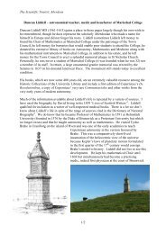
lumen, where bacteria populations grow and the digestive material is contained.
Figure 2-1: Gut structure.
From research of Salmonella Typhimurium behaviour [1, 4-5], the areas of interest are the intestinal
lumen, where the bacteria populations reside, and what the papers refer to as the “membrane”,
which I interpret to refer to the other layers.
In the large intestine alone there are five sections, the ascending, transverse, descending and
sigmoid colons and the rectum. The lumen medium in first two sections, known collectively as the
proximal colon, is liquid and has a pH of around 5-7 [6], whereas the lumen in the distal colon, which
includes the descending and sigmoid colons and the rectum [7], tends to be more solid and have a
pH of 7 or higher [6].
10

Salmonella Typhimurium uses type three secretion systems (see “Biological Background-
Salmonella”) to penetrate the “membrane”. As the mucosal layer is the first barrier round the
lumen, I assume this is where penetration begins.
The mucosa has various specific and non-specific defences. The specific defences include
immunoglobulin-A, part of the complement system (see Immune Response) and T cell populations
[3]. The non-specific defences consist of other innate immune system mechanisms such as
macrophages and other antigen presenting cells [3]. There are also barrier mechanisms; a viscous
mucin barrier and a saliva barrier [3]. These barriers not only provide potentially hostile
environments for some bacteria (the saliva barrier is alkaline), but also have very tight cell
structures, which blocks the translocation of bacteria and the quick turnover of the content of the
mucosal barrier means any bacteria in the barrier won’t be in the same place for long [3].
When considering the defences presented by the mucosal layer, it will be assumed that the
pathogens targeting the tissue will have mechanisms to overcome these barriers. The variation in
the lumen density is of limited importance to the model, however it will govern the diffusion and
movement of nutrients through the environment, which is important as bacteria are attracted to
and require these nutrients to survive. The pH of the environment is one of the controlling factors
with regards to the composition and growth dynamics of the gut bacterial flora [6] and will therefore
need to be considered.
2.2 Native flora composition
The subsections of the intestines have different population levels of different bacteria. The small
intestine contains very little bacteria due to the composition of the lumen medium, which is mostly
acid, bile and pancreatic secretion [8], making it hard for any bacteria to thrive. The large intestine
however has very large populations of various bacteria, with some reaching concentrations of up to
10 12 cells per gram of luminal content [8]. These populations vary as well, with higher populations in
the proximal colon [6].
The variation in species of bacteria in the human body is extensive, with an estimated 400 different
species in the colon alone [6]. The main bacteria in the colon are Bacteroides, Bifidobacterium
bifidum, Coliforms, Lactobacillus, Escherichia Coli, Clostridium, Streptococci, Staphylococcus aureus,
Spirochetes and Enterococcus faecalis [9-12].
Roughly 99.9% of the colonic bacteroides, and 30% of the total gut flora, are anaerboes [6, 13] and
are made up of just four species B. thetaiotaomicron, B. vulgatus, B. distasonis and B. fragilis. It is
suggested that they are the key anaerobes in health and disease [11, 13] and there are
approximately 10 11 bacteroides per frame of lumen medium in the colon [10]. The level of
bifidobacterium varies between 10 10 and 10 11 per gram of luminal medium an adult colon [9-10].
The population densities of Lactobacillus, Streptococci, Coliforms, Escherichia Coli and Enterococcus
faecalis vary between 10 6 and 10 8 per gram of luminal medium [9-10]. The Clostridium population is
just over 10 3 [10]. Staphylococcus aureus forms approximately 24x10 3 per gram of faecal material,
this is a negligible population level when compared to Coliforms, Streptococci and Lactobacillus,
whose populations in the same experiments ranged from 24,000x10 3 to 58,000x10 3 [14].
Populations of Spirochetes are also low [14].
11

2.3 Salmonella
Salmonella heterogeneously expresses both type three secretion systems (TTSS) and flagella. The
type three secretion systems are what allow the salmonella pathogens to penetrate the mucosa
layer of the gut and attack the tissue [15]. During experiments [1], the TTSS were focused on as the
trait effected by phenotypic noise and causing self-destructive cooperation. The results of the
experiment showed that 15% of the final pathogen population in the gut lumen were phenotypically
TTSS-1 + (expressed the type three secretion systems) and nearly 100% of the bacteria in the gut
tissue were TTSS-1 + , while the all or the majority of the bacteria remaining in the gut lumen were
found to express TTSS-1 - (did not express the type three secretion systems). It was also found that
the intensity of the inflammation increased as the number of bacteria capable of expressing the
TTSS-1 + phenotype increased. The high concentration of bacteria with the TTSS-1 + phenotype in the
gut tissue indicates that it is an important factor for allowing the invasion of the tissue. However,
the paper [1] also states that there are likely to be other factors which are important for tissue
invasion.
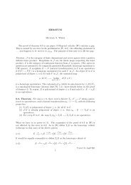
Type three secretion systems refer to a dynamic whereby, when a salmonella population infects a
host, some of that population inject various effectors into the membrane layer, which causes it to
engulf the pathogen [4]. Once a pathogen has made host cell contact, it begins injecting the effector
pool within a few seconds. As the effectors are injected, the host begins to ruffle and engulf the
pathogen and as this happens, the injection process accelerates as more TTSS-1 injectors are
activated. Salmonella typhimurium pathogens require roughly 80 to 200 seconds to deplete their
pool of effectors [4]. The ruffling begins approximately 20 seconds after a pathogen has docked with
the host membrane [16] and halts between 30 and 60 minutes after the invasion is complete [4].
Figure 2-2: Salmonella TTSS-1 injection and consequential engulfment.
Once the salmonella pathogen has been engulfed by the host, the TTSS-1 process finishes and TTSS-2
process begins. TTSS-2 is the process the pathogen undergoes after it has been engulfed and it
involves injecting further effectors, in order to prevent destruction of the pathogen in its new
environment. Once the pathogen has been engulfed by a host cell, it begins replicating in that cell
[4] and eventually induces apoptosis (see “2.5 Cell Life Cycle”) in the cell, which is apparent 2 hours
after infection of the cell [17]. The survival and ability to thrive of salmonella pathogens within a
host cell depends on the type of cell. The cells are normally macrophages, but the ability of the
pathogen to control the cell and grow depends on where that macrophage originated [18].
Schlumberger and Hardt [4], also mention that there are many unknowns with regards to this
behaviour of salmonella pathogens. The questions noted are: “Are all the TTSS-1 effectors injected
at the same time or is there a hierarchy of injection?”, “How do local effector concentrations change
12

over time?”, “How does this affect local concentrations of signalling molecules within the host cell?”
and “how do these signalling cascades cooperatively lead to responses such as engulfment?”
Modelling possible answers to these questions would be interesting, though, in order to answer the
protein/molecule level questions, one would need to focus more on a molecular level model (as
opposed to the cellular level model I will be creating). However, the model will provide various
sacrificing mechanics, so the timing of sacrifices can be explored.
2.4 Factors affecting bacteria
As previously mentioned, the pH of the environment affects the bacteria. There are many other
factors, falling into the categories of physiochemical, host-bacteria interactions and microbemicrobe
interactions. The pH level is one of the four physiochemical factors, the other three being
nutrient supply, oxidation-reduction potential and oxygen tension [6]. In addition to these factors,
the temperature of the environment also has a large influence on bacterial growth and survival [19-
20].
The pH and nutrient levels both have a large effect on the population counts of bacteria as nutrients
are required for growth and duplication and a suitable pH is required for survival. As previously
mentioned, the pH of the intestine is maintained at 5-7 in the proximal colon and at 7 or higher in
the latter sections [6], mediated by secretions from other organs and by bacteria [10]. The level of
nutrients is dependent on what the host consumes and how much of the nutrients are absorbed in
previous parts of the digestive system.
Oxygen tension refers to the level of oxygen in a medium. Salyers AA. states that if oxygen is
present in the digestive medium then colonic bacteria will not grow [11], this has been supported by
experimental data [19, 21]. However, the reference works do show that some of the bacteria can
survive some exposure to oxygen. The fact that the bacteria does not thrive in oxygen leads me to
believe that it is normally not present and is therefore not relevant to the model, unless some other
problem with the host exists.
Oxidation-reduction potential is a measure of the potential of a species to acquire additional
electrons. Studies show that growth of anaerobic bacteria is only slightly affected by this factor [21].
Although the paper only looks at one of the four specific key types of bacteria of the colon, B.
fragilis, it shows similar results for all three of the anaerobic bacteria tested. I will assume that the
other anaerobic bacteria behave in a similar manner and therefore this factor will not be considered
important for this model.
The host-bacteria interactions which control the gut bacteria composition are saliva, bile, gastric
secretion, pancreatic secretion and immune systems. Saliva, bile, gastric secretions and pancreatic
secretions all have a large effect on the small intestine environment, preventing substantial bacterial
growth [6, 8]. In the more intensely populated large intestine, there is only the saliva barrier, which
forms part of the mucosa layer of the gut. However, the environment will still be influenced by the
elements affecting the small intestine lumen medium as it will eventually flow into the large
intestine. The immune properties of the gut mucosal layer have been mentioned and more
information on the immune system function follows this section.
13

The microbe-microbe interactions affecting colonic bacteria composition are bacteriophages,
bacteriocines and toxic metabolites. Bacteriophages are viruses which attack bacteria. For the
purposes of the model, these will also be omitted from the model as they are external influences not
normally found in the environment. One definition of toxic metabolites is “potentially harmful
chemicals produced through normal function” [22]. As this factor falls under microbe-microbe
interactions, I will assume that it refers to toxic metabolites produced by the bacteria. This makes
toxic metabolites very similar to bacteriocines, which are chemicals produced by bacteria to inhibit
the growth of related or similar bacteria. Bacteriocines and toxic metabolites will be important in
the model, if various types of native microflora are to be individually represented.
2.5 Cell life cycle
Organisms can be made up of either a single cell or multiple cells. Single cell organisms are called
prokaryotes and salmonella and most of the native microflora in the human gut are prokaryote
organisms. Multiple cell organisms are called eukaryotes, which is what all more complex organisms
are, ranging from yeasts, such as Candida Albicans, to human beings.
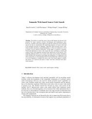
All prokaryotic cells (which the native bacteria and salmonella pathogen are), follow a very simple
life cycle of growth, DNA synthesis and cytokinesis. During the growth stage, the cell performs its
normal tasks and gains energy. The second stage, synthesis, is when a cell begins to duplicate its
DNA strands and otherwise prepare for cell division. The final stage, cytokinesis is when the cell
actually divides, producing a new cell. In microbiology, the generation time of a cell is the period of
time between two cell divisions, the duplication time is how long it takes an entire population to
double. Figure 2-3 shows the life cycle and gives an idea of the time span of each stage. It should be
noted that the rate of division is not constant, with most bacteria moving through a lag phase,
where little division occurs and, if conditions are favourable, enter the exponential phase where cell
division increases dramatically.
Division
Synthesis
.
Figure 2-3: Prokaryote Life Cycle.
There are two ways in which a cell can die. The first is necrosis, which occurs when a cell becomes
damaged in some way or cannot get the nutrients it requires to survive. The second is apoptosis,
which is also known as programmed cell death and occurs generally for the benefit of the organism
the cell is a part of. It can be triggered by the cell itself, surrounding tissue or an immune system cell
and is normally induced when a cell becomes irreparably damaged (e.g. DNA damage or viral
infection).
In order to move and therefore gain the nutrients they require, bacteria have string-like flagella.
They can use these to propel themselves forward, by counter-clockwise rotation or, rotate them
clockwise, causing a “tumble” and therefore a direction change. As bacteria near chemo-attractants,
.
.
Growth
14

such as its food source, swimming becomes more regular than tumbling and vice-versa. This
variation in swimming/tumbling frequency helps keep bacteria in areas with higher nutrient
concentrations.
2.6 Immune response
The immune system consists of various types of cells, each acting independently on simple, local
rules [23]. It has a series of complementary natures, which are self/non-self recognition,
innate/acquired immunity and cell-mediated/humoral immunity [24].
The higher level defences of the immune system consist of skin, sneezing, acidic compounds
generated by the body on skin and hair follicles also provide general ways to expel or destroy
bacteria. The more interesting of these higher-level systems, with regards to this project, are the
sticky mucus in the respiratory and gastrointestinal tract, which can trap many micro organisms.
Also, the normal floras which inhabit the body are of interest as they will work to destroy any other
bacteria which try to occupy the same ecological niche in the body as they are.
The only cellular agents of the innate and active immune systems which are important for selfdestructive
cooperation and type three secretion systems are the macrophages, which pathogens
occupy after penetrating the intestinal membrane. However, this portion of a pathogen’s existence
will not be considered for simplicity.
As part of the innate immune response, macrophages release various inflammatory mediators,
which work to kill the cause of the immune reaction and alert other immune cells to the detection of
a problem [25]. In the early stages, the release of mediators such as leukotrienes, prostaglandins
and histamine is stimulated by infection or injury. As these mediators bind to receptors on the
endotherial cells (which line the capillaries), the cells begin to contract, making it easier for
leukocytes (white blood cells) to perform extraversion (move through the capillary “walls”). A full
list of inflammatory response functions and chemical mediators can be seen in table 2-1.
15

FUNCTION MEDIATORS
Increased vascular permeability of small blood
vessels
Histamine, Serotonin, Bradykinin,
C3a, C5a, PGE2, LTC4, LTD4,
Prostacyclins, Activated Hagerman factor,
High-molecular-weight kininogen fragments,
Fibrinopeptides.
Vasoconstriction TXA2, LTB4, LTC4, LTD4, C5a, N-formyl peptides
Smooth muscle contraction C3a, C5a, Histamine, LTB4, LTC4, LTD4, TXA2,
Serotonin, PAF, Bardykinin
Increased endothelial cell stickiness IL-1, TNF-α , MCP, endotoxin, LTB4
Mast cell degranulation C5a, C3a
Phagocytes
Stem cell proliferation IL-3, G-CSF, GM-CSF, M-CSF
Recruitment from bone marrow CSFs, IL-1
Adherence/aggregation iC3b, IgG, Fibronectine, Lectins
Chemotaxis C5a, LTB4, IL-8 (and other chemokines), PAF,
Histamine, Laminin, N-formyl peptides, Collagen
fragments, Lymphocyte-derived chemotactic
factor, Fibrinopeptides
Lysosomal granule release C5a, IL-8, PAF, most chemoattractants,
phagocytosis
Production of reactive oxygen intermediaries C5a, TNF-α, PAF, IL-8, Phagocytic particles, IFN-γ
increases Fc receptor expression
Granuloma formation IFN-γ, TNF-α, PGE2, IL-6
Pyrogens IL-1, TNF-α, PGE2, IL-6
Pain PGE2, Bradykinin
Table 2-1: Inflammatory response functions and mediators (information from the work of V Stvrtinova et al.
[26]).
The inflammatory response will continue until the invader is destroyed. In the case of salmonella,
the invaders would be the cooperative pathogens who are attacking the tissue. T-helper cells are
responsible for mediating the end of the immune response. All cells involved in the immune process
are “programmed” to die, unless they receive signals from other cells to stay alive. It is the T-helper
cells that emit these “stay alive” signals. This method of cell regulation is called apoptosis.
In terms of the salmonella infection, the main point of interest is the self-cooperative and
destructive behaviour exhibited by some members of the invading population, which induces an
inflammatory immune response in the host [1]. This inflammatory response has been shown to
benefit the invading population, due to environmental changes suppressing the native microbe
populations [1, 5]. However, as is shown above, the inflammatory response alone is a very
complicated process and therefore it is likely only a partial or simulated model of this response will
be included in the model.
16

2.7 Environment and bacteria data
I will now outline the test values I will use for the biological properties in the model. The figures
below are what I am considering the biological norm. As you will notice, I am lacking some data for
certain bacteria in the colon, which is because I simply could not find the data. A lot of the data
below also don’t refer to the bacteria’s behaviour in the colon or gastric juices specifically, so I had
to generalise based on the information I could find. I am not convinced these values will provide an
accurate simulation of the infection dynamics, as bacteria behave differently with the slightest
environmental change, be it pH, temperature, nutrient level or even what is providing the nutrients.
However, these values do provide a good starting point for defining a range of native bacteria and
the salmonella pathogens.
Normal colon temp: ~36 o C. The reference, [27], actually states these as the rectal temperature,
however, from the values I found, this is the closest body region temperatures I found.
Feverous colon temp: High of 39.4 o C [28]
Normal colon pH: 5 - 7+ [6]
Cooperator injection activation: A few seconds [4]
Cooperator effector pool depletion: Between 80 and 200 seconds [4]
Host membrane ruffling: Begins approx 20 seconds after injection starts, ends 30-60 minutes after
invasion is completed.
Infected host cell apoptosis: Less than 2 hours after infection.
Salmonella generation time: ~31 minutes (derived from data from [29-30])
Salmonella pH: Survives between 3.8 and 9.5. Optimum pH is between 7 and 7.5 [31-32].
Salmonella temperature tolerance: Survives between 7 o C and 49.5 o C, but below 15 o C, growth rate is
greatly slowed. Optimum temperature is 35 o C - 37 o C [32].
Bacteroides
B. thetaiotaomicron generation time: ~52 minutes [33] (average)
B. vulgatus generation time: ~53 minutes [33] (average)
B. distasonis generation time: ~83 minutes [33] (average)
B. fragilis generation time: ~32 minutes [33] (average)
Bacteroide pH: Survives in pH levels above ~6 [33]. The paper, [33], also shows increased growth as
the pH increases up to 6.7. As the maximum pH of the colon (as mediated by the body) is just over 7
[4], I will assume that the native flora will continue to increase in growth rate until around 9 and
above 5.5. The optimal pH will be considered to be 6.7.
Bacteroide temperature tolerance: The work of Hoffmann and Justesen [19] indicate that in certain
substances, the bacteroides seem to survive longer in low temperature conditions, decreasing as the
temperature rises. However, Hagen et al. [34], show that in other substances, the survival rate at
certain temperatures can vary greatly. As there is a tremendous amount of variation and I am unure
of the relation of any of the substances used in the experiments to the colon lumen medium, I will
assume a survival between 3 o C and 41 o C. Also, as bacteroides thrive in the colon environment, I will
assume an optimal growth temperature of 36 o C.
Bifidobacterium bifidum generation time: ~98 minutes (derived from [35])
Bifidobacterium bifidum pH: Optimal ~6.75 [36]. Survives between 2 and 9 [36].
Bifidobacterium bifidum temperature tolerance: Optimum ~39 o C and Survives between 20 o C and
45 o C [36].
17

Escherichia Coli generation time: ~29 minutes (average value from data in [30])
Escherichia Coli pH: Optimal 6-7 [37].
Escherichia Coli temperature tolerance: Survives between 7-8 o C and 46 o C. Optimal 37 o C [37].
Clostridium perfringens generation time: ~20 minutes (from data in [38-39]).
Clostridium perfringens pH: Optimal is between 6.0 and 7.0 [39].
Clostridium perfringens temperature tolerance: Survives between 12 o C – 50 o C, optimum
temperature is between 43 o C and 47 o C [39].
18

3. Related Work
I have taken some time to examine some existing biological systems models and simulators. The
purpose of looking at these existing related systems is to see how others have approached modelling
biological systems and cell interactions, with the goal of implementing some of the features of my
own model in a similar fashion and also providing insights into other features which I may not have
otherwise considered.
The existing systems I found tend to focus on immune system simulation. Though my project is
focussed more on bacteria population dynamics, the cell interaction processes and how actions are
determined will still be applicable. Additionally, some of the systems focussed on simulating
immune responses to specific pathogens, which could also provide some useful information on
pathogen simulation.
CAFISS
CAFISS (complex adaptive framework for immune system simulation) is a Java program, developed
by Joc Cing Tay and Atul Jhavar, which uses complex adaptive systems (CAS), developed by John
Holland, and some features of cellular automata, genetic algorithms and Holland classifier systems.
It has been implemented in an event driven and distributed manner, with each agent having its own
processing thread [23]. The implementation described in this paper, [23], is designed specifically to
simulate the immune response to HIV.
One of the main motivating factors of this system appears to be to observe the feasibility and
effectiveness of using complex adaptive systems, specifically Holland classifier model, to model
biological systems, instead of just ordinary differential equations or cellular automata. A classifier is
a simple if-then rule and the classifier system is designed to learn these rules over time, guiding its
performance. The agents of the system receive environment information, process it using a rule
base, then act. The rules are weighted using algorithms, based on performance. The rules and their
strengths are not global, but specific to each agent in the system.
CAFISS uses a grid structure to represent the body, with each grid location containing a number of
cells. These cells can be different and all express autonomous behaviours. Then, over time, viral
cells are added to grid locations at random and the two cell types then compete to destroy one
another. The specifics of the interactions and dynamics of this competition are unknown, though
they probably emulate the active immune system behaviours.
The distributed nature of the system is interesting as it gives each agent the ability to process its
behaviours independently and maintains the immune system property of no central control and also
eliminates global times steps. Another point of interest is the apparent disregard for simulating the
environment. The grid like structure gives some boundaries for cell locations, but is not
representative of any particular environment, suggesting that the focus of the model is solely on the
immune system – pathogen interactions, almost completely ignoring other body functions and
native agents who may influence the model. However, even with these omissions, which I would
assume would greatly affect the behaviour of the system, when the results of testing were
compared to actual biological data, they were found to be reasonably accurate and the authors state
that the system shows promise for CAS biological systems models [23].
19

IMMSIM and Variants
The original IMMSIM program was written in ALP2, by Philip E. Seiden, which meant there is no
scope for dynamic memory allocation and limited the simulation to small scales [23]. The system
was re-implemented in C by F. Castiglione and had parallel computing features added. The parallel
nature indicates that C-IMMSIM also adheres to the decentralised nature of the immune system. As
mentioned before, IMMSIM focuses on the active immune response and more specifically, the
humoral response, though the system is designed in such a way that the immune reactions to
different pathogens can be simulated.
One of the most interesting features of IMMSIM, is the bit string representation of receptors. A B
cell, for example, would have its receptor represented by a bit string and a MHC II molecule,
represented in the same way [40]. The receptor would match the pathogen whose presenting
molecule is the complement of the receptor bit string, or close to it using some affinity metric. This
bit string representation of receptors and molecules was first applied by Seiden and Celada [23] in
the original IMMSIM and provides an accurate simulation of self/non-self discrimination. The
technique has been used by many other systems [23, 40].
The method used to determine the actions of agents is also interesting. Instead of rules being
chosen based strictly upon states, a set of possible actions for each agent is generated each cycle
and then a single action chosen using probabilities. This provides a more random, though still rule
based, expression of behaviours.
The system also uses a grid structure for the environment, though the grid is hexagonal, which
allows agents to move to 6 possible locations instead of 4, as it would be for a square grid.
Increasing the degrees of movements gives a more accurate representation of the infinite degrees of
movement available to the cells in reality. The environment, as with CAFISS, does not seem to
adhere to any specific body region, with the various cells being “injected” into cells, as opposed to
realistic simulation of cell movement e.g. immune system agents moving from capillaries to tissue
etc, but again has very positive testing results and has been used to investigate various biological
interactions [40].
SIMMUNE and CyCells
These two systems are very similar in that they attempt to create more general models of cell and
molecule interactions [40], allowing users to define behaviours at both levels. Both models are
implemented on a 3 dimensional grid, though SIMMUNE also allows the user to define
compartments of the grid to represent different parts of the environment and which cells can move
between the compartments and at what rate. This flexibility of defining the molecule and cell
interactions means that the systems can be used for more than just immune system simulation [41].
I am unsure how much CyCells allows user customisation of the environment, but due to its
generalised nature and the possibility of it being used to model more than immune system
responses [40, 42], it is very likely that some kind of customisation of the environment is possible.
The actions of cells in SIMMUNE are determined using what they call “cellular stimulus response
mechanisms” [41]. These are effectively series of if-then statements, with cells performing actions
when certain conditions needed to trigger that action are met. The conditions part of the
action/decision process consists of one or more conditions linked with logical AND or AND NOT and
the action part consists of one or more actions [41]. Cell actions in CyCells operate in a fairly similar
20

way, using a “sense-process-act” model for cell behaviours [40, 42]. This model for cell actions is
made possible by CyCells approach to the immune system modelling, continuously representing
molecular concentrations and having cells react to and modify those concentrations [42].
The interesting feature of these models is the method of decision making for cells, which seems to
work on the sense-process-act model in both systems. Although this behaviour model is not ideal
for all cell behaviours, such as apoptosis, it will be useful to implement a similar system for
determining agent movement, effecter secretion by salmonella agents and other similar processes.
Innate Immune Response (NetLogo simulation)
This model of the innate response was created by Gary An and simulates the interface between the
endothelial cells that line capillaries, and blood-borne inflammatory cells and mediators of the
immune response. The model is freely available online from the NetLogo website.
NetLogo restricts the simulation to a 2 dimensional grid. The model has a series of variables
assigned to each patch, each representing one of the immune system mediators, however, the
author admits that the actions of these mediators is incomplete. To simulate infections and injuries,
the model uses patch variables and cellular automata techniques.
The agents in the model consist of endotherial cells, neutrophils, monocytes and macrophages.
These all react to the mediator concentrations on the patches. This is similar to the sense-processact
model used in other biological systems models, though it appears there is no separation of sense
and act behaviours, i.e. a single cell will sense then act, then next cell etc.
BacSim
BacSim is an agent based model of bacterial population growth. It models the growth dynamics at
the cellular level, with each of the cells being an individual agent and operating on a 2D plane, which
is coated in some kind of nutrient source for the bacteria agents [43].
Some of the most interesting aspects of the BacSim model are the details on how they handled
certain biological functions. For example, the rate at which a cell consumes the nutrients it uptakes,
is constant, with the growth rate, being a function of that consumption rate, the rate of nutrient
uptake (which is proportional to cell surface area) and some maximum growth rate. Also, the
diffusion mechanism for nutrient spread through the environment is of interest. A second-order
approximation is used with weighting applied to the nine cells, based on nutrient concentration,
involved in the diffusion shown in figure 3-1. [43]
1 4 1
4 -20 4
1 4 1
Figure 3-1: Diffusion weights in BacSim.
Kreft et al. [43] also cite the work of Donachie, which states that the triggering of DNA replication
(DNA synthesis) in a cell occurs at masses which are multiples on one mass [44]. As the mass of a
cell is relative to the resources it consumes, this makes it clear that there is a direct correlation
between nutrient level and cell division.
21

4. Approach
Biologists and mathematicians normally use ordinary differential equations are used to model
biological systems, which give empirical data describing a host-pathogen interaction and outcomes
of the interactions. The use of ordinary differential equations is useful for this purpose as a lot is
known about them and how they behave and they require few parameters [45].
However, ordinary differential equations do not account for spatial information, which means they
assume that populations are homogenous and distributed equally across the simulation space, an
assumption which could heavily influence the outcome of the simulation [45]. To account for this
weakness, partial differential equations can be used. However, as the equations get more
complicated, this and other advantages of partial differential equations quickly become
overshadowed by the disadvantage of the complexity.
The main problem with these approaches is that they only provide data for a generalised, average
situation. This is because they don’t take into account the individuality of the agents involved in the
system (pathogens, native floras, immune system agents etc) or the spatial information.
In an attempt to address these issues, John Von Neumann and Stanislaw Ulam introduced agent
based modelling as an approach to simulating biological systems [45]. As they were specifically
designed for implementing biological systems, many successful systems, for teaching and research
purposes, have been completed in the past using agent based modelling techniques [23, 41, 45-48].
Agent based models are stochastic models which can be used to describe populations of interacting
agents using simple rules, which dictate the behaviour of those agents. As each agent responds
individually to changes in the environment (or other cues), allowing emergent behaviours to
develop, so the simulations become more valuable for studying autonomous systems. Additionally,
the rules of agent based models tend to relate to the language used to describe the model, so it is
easier to relate agent based models with the real world than it is mathematical models.
The weakness of agent based modelling lies in translating the results into natural language. When
using differential equations, the worst case scenario would be a large set of complicated equations,
but the equations could be reorganised into a more meaningful manner. With agent based
modelling, many of the intricacies of the system lie in the code and implementation strategy, which
could be overlooked when translating the results into words or trying to explain any emergent
behaviours [45].
In order to create an agent based model, an object oriented approach would be required in order to
create separate classes for each agent and therefore define individual behaviours, properties and
variables (for flags e.g. if an invading agent has been marked by the immune system). There are
many object oriented languages available, but I already have considerable knowledge of Java and I
don’t believe learning other languages would provide any benefits which would outweigh the time
spent doing so.
In addition to the option of using Java to program the model from scratch, there are tools designed
specifically for creating agent based models such as NetLogo and SeSAm. These tools provide an
interface for creating agents and environments. This means that instead of writing a complete class
for each agent, it would be done automatically when a new type of agent is defined, although there
22

are libraries, such as SWARM, which provide frameworks for agent based modelling in object-C and
Java, the modelling tools also provide built in visualisation functionality. These visualisation
functionalities are the main reason I am considering using NetLogo or SeSAm as I have limited
knowledge of graphics programming, even in Java, though my experience is sufficient to know that
creating a suitable visualisation of the model would be a time consuming process. As this project is
not an exercise in graphics programming, I wish to limit the time spent on such periphery coding,
especially when sufficient systems already exist.
I have used NetLogo before, so if an agent based modelling tool was to be used, I would probably
opt for it. I have taken a look at SeSAm and it provides some good interface tools for creating
agents, with states and rules represented in a UML style diagram, as opposed to the code-based
approach of NetLogo. Although this is probably a very useful feature for the less computer-oriented
individual, I have a good programming background so it doesn’t present that much of an advantage.
The use of SeSAm is further disadvantaged by the fact that I would need to learn the rest of the
interface too, such as programming the environment and agent reactions.
An unfortunate result of using one of these agent based modelling tools is that my control over the
basic interactions and data processing will be limited. For example, when looking into existing
biological systems models, it appears that the developers attempted to perform the decision making
for cells and once all agents had decided on an action, perform those actions stochastically. I know
NetLogo provides stochastic mechanisms when iterating through agents, though separating decision
making and action performing may be complex and could lead to messy code. This is made more
likely by the fact that NetLogo code is created in one file. Careful planning and thorough
commenting will be needed to maintain readability.
Should Java or some other object oriented be used, multi threaded programming techniques could
be implemented to provide stochastic action performing. The separating decision making from
action performing would still require the code to be written in a specific way, so there would be no
difference in work required to implement that feature. Using Java would also allow the creation of
separate classes and the implementing of certain processes in those classes, making clear code
maintenance easier. Portability of the code is equal as NetLogo is Java implemented and allows the
model to be exported as a Java applet.
When all of the above is considered, I believe a NetLogo implementation of the model would be the
best option.
23

5. Required Behaviour
Table 5-1 shows a list of requirements and the priorities I have assigned to them. Although this is a
requirements list, some design decisions were made so I have also included notes explaining how
the decisions I made lead to the priorities some requirements have been assigned or how the
decisions lead to the existence of the requirement.
Ref. Description Priority Notes
1 Environment
1.1 Proportional representation of lumen
and membrane.
HIGH
1.2 Gut lumen
1.2.1 Nutrient level HIGH
1.2.2 pH level HIGH
1.2.3 Influence on pH from previous areas of HIGH
digestive system
1.2.4 Nutrient diffusion MED
1.2.5 pH diffusion MED
1.2.6 Flushing
1.2.6.1 Remove percentage of bacteria
population in lumen per flush
MED
1.2.6.2 Diffuse nutrients MED
These requirements would provide a
basic simulation of a flush.
1.2.6.3 Diffuse pH MED
1.3 Membrane Layer
1.3.1 Ability to block bacteria HIGH
1.3.2 pH Level MED Although the pH level in the mucosa
barrier provides a hostile environment
for bacteria, none of the bacteria will
enter the area in the model. The pH of
the membrane layer will be used solely
to influence the pH of the lumen.
2 Bacteria
2.1 General Behaviours
2.1.1 Movement towards high nutrient
HIGH
2.1.2
concentrations
pH control (through secretions) MED
2.2 Individual Cell Growth Dynamics
2.2.1 Growth rate (cell size) relative to
nutrient uptake rate
HIGH
2.2.2 Nutrient uptake rate HIGH
2.2.3 Temperature affect on growth and
survival
HIGH
2.2.4 pH affect on growth and survival HIGH
2.3 Population Dynamics
2.3.1 Division mediated by cell size (growth) HIGH
2.3.2 Death by necrosis HIGH
2.3.3 Death by apoptosis HIGH
24

2.3.4 Cell death creates additional nutrients
for other cells
2.4 Native Microflora
2.4.1 Representation of generic native flora,
with varying properties.
2.4.2 Inflammation affect on growth and
survival
2.5 Salmonella Typhimurium
2.5.1 Representation of pathogens with type
three secretion systems
2.5.2 Representation of pathogens without
type three secretion systems
2.5.3 Dynamics for pathogens with TTSS
penetrating the membrane
2.5.4 Time scale dynamics of TTSS pathogen
mucosa invasion
2.5.5 Inflammatory response triggered when
TTSS pathogens interact with
membrane
2.5.6 Removal of salmonella TTSS-1
pathogens once invasion of membrane
is complete
3 Immune system
3.1 Inflammatory response affect on
environment temperature
3.2 Specific modelling of inflammatory
response dynamics
4 Visualisation
MED
HIGH It would be ideal to vary the properties
and numbers of native microflora in a
way that accurately represents the
average populations of certain
bacteria in the gut lumen; however,
due to lack of data, this is not possible.
HIGH
HIGH
HIGH
HIGH
HIGH
HIGH
HIGH
HIGH
LOW
4.1 Visualisation of lumen and membrane HIGH
4.2 Visualisation of native microflora and
pathogens
HIGH
4.3 Visual indication of inflammation HIGH
4.4 Visualisation of nutrient levels in lumen MED
4.5 Visualisation of pH levels in lumen MED
4.6 Visual engulfment of pathogens when
TTSS-1 effectors are injected
LOW
Table 5-1: Required model behaviours and their priorities.
25

6. The Model
The following section outlines the basic program flow and the equations and representations that
will be used to model and provide visualisation of a salmonella typhimurium infection. Also included
are some base values, based on my research, which will provide initial parameters for the behaviour
of the model.
6.1 Interface
The interface has been designed with NetLogo in mind as the implementation method. The reason
NetLogo has to be considered is because it only allows one interface screen, no tabs or other forms
of separating interface components are available. In addition, many interface components cannot
be resized to take up less space and if they were, the labels indicating the function of the component
would be illegible.
In light of these facts, the interface will undoubtedly take up more space than most displays will be
able to show at one time. So, I decided the best approach would be to group together input and
output regions, attempting to allow easy viewing of the visualisation, alongside any graphs and
empirical data outputs and basic model controls (stop/start etc). This will make controlling and
observing the results of the model easier. The fact that most of the parameters will be out of view
while the visualisation is in view is justified as it is unlikely they will need to be changed while the
model is running.
6.2 Program flow
The flow of the program is not especially important due to the way I intend to enable the adding of
bacteria and pathogens. That is, no bacteria agents will be present at the beginning of the
simulation, which will allow the nutrient and pH concentrations in the environment to settle, based
on the rules I specify. This means that the whether the environment and agents are updated first
should not have a large affect on the model as it would only be of significance on the first cycle of
the simulation, should the bacteria be present on that cycle.
A single simulation cycle will represent 6 seconds. This value was chosen as it provides nice intervals
for minutes (10 cycles = 1 minute) and hours (600 cycles = 1 hour) and still maintains a reasonable
speed in terms of actions of the model (bacterial movement etc). Figures 6-1 to 6-4 show the flow of
the program and what the stages will involve.
26

Pause
simulation
Update pH
levels
Initialise global
variables
Figure 6-1: Setup procedure.
Interruptible Region
Check halting
conditions
Resume
Figure 6-2: Main simulation cycle.
Update nutrient
concentrations
Figure 6-3: “Update Environment” stages.
Move agents Consume
nutrients
Check for and initiate new
sacrifices among pathogens
Figure 6-4: “Update agents” stages.
Draw
environment
Update data
outputs
Initial
Entry
Update
environment
Update sacrifice
processes
Initialise
environment
Update
visualisation
Update inflammation
and temperature
Check for
deaths
Update agents
Check for
divisions
Check for and
perform flushing
27

6.3 Environment
Lumen and membrane
The requirements state that a representation of the lumen and membrane is needed to provide
areas for the bacteria to perform the actions required for the simulation. The environment is to be
represented in a 2D grid structure. The 2D nature is inaccurate in terms of reality; however, time
scale limitations mean that a 3D implementation is simply not feasible and many other systems have
implemented biological models on 2D grids with a high level of success. Each location in the
environment grid will contain agents and have “type”, “ph level” and “nutrient level” properties.
The “type” property will state whether the cell is part of the lumen or membrane, allowing detection
of borders for controlling agent behaviour. The “ph level” and “nutrient level” properties will allow
controlling of those environment factors.
In order to prevent all agents moving to and occupying a single grid location, which would be
unrealistic, each grid location will be restricted to containing 2 bacterial agents. This means a certain
grid size is needed in order to accommodate the agents in the model, however, the number of
agents cannot be controlled as they divide and die based on behaviour and environment properties.
The size of the grid will be approximately 150x80 cells, giving a rectangular grid area which provides
a large number of cells for bacteria to occupy.
It will be necessary to represent the layers so that sufficient space is available to allow the agents to
function. To that end, the majority of the environment space will be devoted to the lumen area.
The membrane layer will be represented as a layer surrounding the lumen, sufficiently large to allow
visualisation of salmonella pathogen’s type three secretions and invasion process and the pathogen
growth dynamics in the area. I have decided not to implement any representation of the tissue layer
as it would only be required for specific modelling of inflammatory response agents. The
inflammatory response will instead be modelled in a more arbitrary fashion, according to data given
in the paper by Ackermann et al. [1]. The exact method of implementing this dynamic will be
explained later.
Membrane (Mucosa)
Lumen
Figure 6-5: Environment representation.
Flow
28

Grid locations just off the in-flow end of the environment will be assigned random nutrient
concentrations between the maximum and minimum values used to initialise the environment.
This will help ensure a replenishment of the nutrient levels in the model.
As every grid location is affected by and affects its neighbouring locations in terms of pH and
nutrient level, I have decided that the new levels for each grid location on each simulation cycle will
all be calculated based on the existing values. Once all new levels have been calculated, the entire
grid will be updated with the new values.
When the model is initialised, the nutrient level of patches will be 0. As the model runs, nutrients
will be diffused into the environment. Because of this, the model will have to run a few cycles
before bacteria can be added to give the environment time to settle. The pH levels of patches will
be initialised to random values between 6 and 8.
As both nutrients and pH levels are going to be grid location variables, creating a visual
representation for both simultaneously would be difficult. Instead, I intend to implement colour
scaling, which will allow visualisation of one of pH or nutrient level at any one time. Interface
options will allow the user to change which property is being visualised.
Flushing
Flushing dynamics will imitate the effects of the host excreting waste and will occur at regular
intervals. The intervals will be determined by two user defined values, specifying the minimum and
maximum time between flushes. The exact values to be used for my experiments will be obtained
through testing; though will likely begin at around 2 hour intervals (1200 cycles).
When a flush occurs, a proportion of the bacteria in the simulation will be removed at random. The
size of this proportion will be a simulation parameter, adjusted during trial and error testing once
implementation is complete to find a suitable value.
In addition to removing some the agents, several pH and nutrient diffusion operations will be run, in
order to alter nutrient distribution and simulate the lumen medium being moved through the
digestive tract. Again, the number of diffusions to be performed will be determined through trial
and error testing, though the initial value will be such that the number of diffusions is equal to the
number of columns in the environment grid, therefore diffusing across the entire environment.
6.4 Bacteria
Movement
In order to grow and survive, the bacteria in the model will need to find and consume nutrients. In
reality, cells are attracted to certain chemo-attractants, which for bacteria are energy sources.
Bacteria movement consists of either moving their flagella to swim in the direction they are facing or
rotate and change direction, both actions requiring one “stroke” of the flagella. These two actions
will be considered to be the possible “move” actions. Based on this information, for every
simulation cycle, the code will find the neighbouring patch to each bacteria agent, which has the
highest nutrient concentration. The bacteria will then rotate to face or move to this patch.
31

without major performance issues. So, I decided to proportionately represent the bacterial agents,
but in lower numbers. However, this means that it will not be possible to represent Escherichia Coli
or Clostridium perfringens due to the proportional populations being so low. In order to still provide
a good range of native microflora, I will implement the capacity for 5 types of natives, which will
represent the four main bacteroide strains and Bifidobacterium Bifidum.
The invasion of Salmonella Typhimurium will be initiated using an interface control, so the pathogens
will not be present from the start of the simulation. The reason for this is to give the native
population levels a chance to settle to the environment capacity, which will change from the given
default numbers depending on the model parameters that affect the growth of the bacteria. The
number of pathogens to be created when invasion is initiated will be a model variable specified by
the user and the percentage of that population expressing TTSS will be a percentage specified by the
user, though initial values I will use will be between 20% and 40%, based on research by
Schlumberger and Hardt [4].
6.5 Self-destructive cooperation
Pathogen Behaviour
The self-destructive nature of the pathogens is a result of the salmonella pathogens, which express
type three secretions systems, penetrating the mucosa layer. As it is uncertain what triggers the
invasion action [4], I will implement several methods which could be the case.
The first two methods are suggested by Schlumberger and Hardt [4] and they are that the pathogens
sacrifice simultaneously or by some kind of hierarchy structure, however, whether this is a one-byone
hierarchy or if many pathogens sacrifice at the same level of the hierarchy is unclear, so I will
implement solutions for both approaches, creating a model parameter for limiting the maximum
number of sacrifices for each stage of the hierarchy.
The third of the methods, suggested by Ackermann et al. [1], is to have the sacrifices based on
probability, with each pathogen having a different floating point number, which will be generated
when the pathogen is created between 0.001 and a maximum value, specified as a model
parameter. Random thresholds will be generated on each cycle (between 0 and 100) of the
simulation for each pathogen. If the generated number is less than the pathogen’s value, that
pathogen will begin sacrificing.
The method of my own is to have sacrifices based on the pathogen’s location, so that when they
happen to move past the membrane layer, they will attach and begin invasion.
Once a pathogen is triggered to begin invasion of the membrane, it will take the most direct route to
the closest mucosa layer area. This behaviour is based on an assumed chemo-attractant which
draws the pathogen to the area. Once it reaches the mucosa area, it will wait a single cycle before
initiating injection of effectors. The injection process, as I have already mentioned, takes between
80 and 200 seconds, in terms of the model, this is approximately between 13 and 33 simulation
cycles. The actual time taken by each individual pathogen will be a random value between these
limits.
The membrane invasion behaviour reduces the pathogen population in the gut environment, as the
pathogens are either destroyed by the immune response in the membrane once they invade (if they
35

concentration of 0. Finally, as the nutrient depletion rate of the bacteria are all to be kept the same
and no death dynamics are needed, this factor was also excluded.
The initial populations were obtained by selecting a bacteroide population which, when proportional
levels of bifidobacterium and salmonella pathogens were added, lead to a total agent count of
around 5000.
Results
Figure 7-1: Designed system, visualisation output.
As can be seen in figure 7-1, the bacteria move towards the edges of the simulation, which has a
detrimental effect on the population dynamics.
The pH diffusion almost works as intended, although, as can be seen in figure 7-2, the alkaline
influence from the membrane gives a curve at the top end of the lumen (see highlighted area). This
is caused by the fact that the top-left grid location is influenced by the random lumen pH, meaning
the pH level is more acidic, which has occurred due to coding error. As we move further to the right
of the model, the grid locations get a diffused value of the initial, more acidic pH, but an alkaline
value (from the membrane) between the same random values as was applied to the top-left grid
location, allowing it a greater influence.
Figure 7-2: pH levels with no bacteria.
39

Figure 7-3: pH levels with bacteria (bacteria are hidden)
Figure 7-3 shows the pH concentrations of the grid locations with bacteria present. In order to make
the difference clearer, I disabled visualisation of the bacteria agents. As can be seen, the agents
have an influence on the environment pH, with the average pH of the environment falling from
around 7 with no bacteria to around 6.7 with the bacteria present. The bacterial influence on the
environment pH seems to lower the average pH to almost exactly their optimum pH levels. The
research I conducted did show that the average pH of the colon is in the region of 6-8, making 6.7 an
acceptable level.
Experiment 1-1– Nutrients
In order to solve the nutrient problem, I initially tried different diffusion methods, removing
backwash or simply moving all the nutrient concentrations along the environment, with no diffusion,
just simulating flow. None of these amendments helped and the reason for this occurred to me
while performing various experiments. The bacteria are attracted to high nutrient concentrations,
but after a certain number of cycles, they will have consumed the nutrients in the centre of the
model and the bacteria closer to the left hand side will be absorbing the new nutrients as they enter
the model. This means that concentrations in the middle area of the model will decrease rapidly and
only be replenished by low concentrations of nutrients, which are not consumed by the bacteria to
the left. Eventually, the bacteria will all clump as close to the left of the model as they can, where
the high nutrient concentrations are and consume all the nutrients before they diffuse past the mass
of bacteria.
As the issue is related to the flow dynamic I implemented, it seems the only way to avoid this issue
will be to assign random nutrient values across the model and replenish those values at regular
intervals, thus removing the flow. Nutrient concentrations will now be initialised at random values
between a minimum and maximum, set as model parameters and replenished at regular cycle
intervals, by taking a random value between the minimum and maximum concentration and then
reducing that value to a percentage of it. This percentage factor will also be available as a model
parameter, which can be adjusted for best effect.
40

In addition, diffusion will need to be un-weighted, that is, each grid location will have to diffuse
equally to all of its neighbours. The new diffusion grid is shown in experiment figure 7-4 and shows
a simple diffusion, whereby each grid location maintains 20% of its current nutrients and disperses
the remaining 80% between the 8 neighbouring grid locations. The values in the grid are again
percentages of the nutrients in the centre grid location.
10 10 10
10 20 10
10 10 10
Figure 7-4: New nutrient diffusion percentages.
This new treatment of nutrients also means that flushing has to be changed. It used to use the
diffusion function, which relied on nutrients being introduced at the borders of the model. As
nutrients are no longer introduced in this manner, flushing will now constitute of assigning new
random nutrient concentrations across the environment and running the basic diffusion outlined
above.
For this experiment, the same parameters as outline above were used. Two new parameters were
added to control the new nutrient system. Those are “Replenish-Nutrients-Every-N-Ticks”, which
was set to 100 and “Replenish-Nutrient-Percentage-Factor”, set to 10%. The reason for setting the
replenish interval to 100 is simply that replenishing the nutrients by a small amount every 10
minutes seems reasonable. Due to the way flush cycles are detected, a flush always occurs on the
first cycle of the simulation, meaning that nutrient levels are initialised and diffused. Because of this,
I allowed one cycle to run before adding the agents to the simulation.
Figure 7-5: Visualisation with new nutrient dynamics
41

Figure 7-6: Average nutrient concentration, with new
nutrient dynamics with flushing enabled.
Figure 7-5 shows that the new nutrient dynamics solves the problem of the bacteria bunching
together at one side of the environment. However, due to the lack of information found on nutrient
distribution, it is hard to determine whether or not the new dynamic is accurate. Based on my own
assumptions, there are two possibilities. It could be considered reasonably accurate, if we assume
that the model is focussed on a single environmental niche, where separate groups of the bacteria
would not develop, a behaviour which is observed in most experiments relating to bacterial growth,
though those experiments were not analysed at a level where each individual bacteria cell could be
seen. However, if we assume that we are at the level where groups of bacteria would form, then the
nutrients are too evenly distributed in the model, preventing the simulation of environmental
niches. It makes sense to assume state that the model represents only a single ecological niche as
we can see individual cells, however it was not designed with that in mind.
Figure 7-6, the average nutrient concentration in the lumen medium over time, shows a steady
decrease in the nutrients as the bacteria consume them. The graph also shows that the new flushing
mechanic completely resets the nutrient concentration of the environment. This resetting of
nutrient levels appears unrealistic, but when we consider what flushing is simulating, the movement
of digestive medium through the environment, it may be considered fairly accurate because,
although nutrients are removed during this process, the host will consume more nutrients and those
will eventually be passed to the colon. Also, the nutrient values introduced are random, so different
nutrient levels are introduced on each flush. Therefore, if the initial nutrient concentration of the
environment is considered to be that just after new nutrients are introduced, the mechanic seems
quite reasonable.
The new nutrient diffusion and replenishment values, although biologically debateable, provide a
stable situation for bacterial agents to operate and will therefore be used for the experiments later.
42

Experiment 1-2- pH
In order to solve the pH issue, I created a special case check for the top left of the model, whereby if
the current column is 0 and the lumen row is row 4 or lower, the random pH influence uses the
membrane range instead of the lumen range to determine a random value. For this experiment, the
model parameters specified at the beginning of this section and the modifications for experiment 1-
1 have been used.
Figure 7-7: pH levels with no bacteria and new diffusion.
Figure 7-7 shows the pH levels of the model with no bacterial agents present. As can be seen, the
pH gradient from top to bottom appears more accurate, with the alkaline membrane influence
forming no curve from left-to right. This indicates that the random influence values for the top 5
rows (rows 0 – 4) of the model adhere more to what the rest of the model predicts and therefore
seem more accurate and will be used for the experiment phase.
7.2 Phase 2 – Bacteria Population Dynamics
This phase is to ensure that bacteria population proportions do not fluctuate too much when there is
no inflammation to assist the pathogens. Also, the experiments will ensure that the bacteria growth
patterns follow known patterns. This will involve trial and error testing, adjusting the maintenance
rates for the bacterium. For these experiments, all varieties of bacterial agents will be added and
their population monitored for the duration of the model is running. In order to get accurate
population counts over time, sacrificing of pathogens and inflammation are disabled.
Inputs
Model runtime: 5500 cycles (approx 9.1 hours)
Visualisation Parameters
Env-Visualistion-Mode – Nutrient Concentration
showPathogens – On
showBacteroides – On
showBifidobacterium – On
Environment Parameters
Env-Base-Temperature – 36
Initial-Env-Nutrient-Concentration-Min – 0
Native Parameters
Initial-Bacteroide-Pop – 3000
Initial-Bifidobacterium-Pop – 1948
Initial-Native-Nutrient-Concentration-Min – 40
Initial-Native-Nutrient-Concentration-Max – 100
BFragilis-Base-Uptake – 0.87
BDistasonis-Base-Uptake – 0.335
BThetaiotaomicron-Base-Uptake – 0.534
BVulgatus-Base-Uptake – 0.525
43

Initial-Env-Nutrient-Concentration-Max – 100
Replenish-Nutrients-Every-N-Ticks – 100
Replenish-Nutrient-Percentage-Factor – 10%
Flushing Parameters
Enable-Flushing – On
Min-Cycles-Before-Flush – 1050
Max-Cycles-Before-Flush – 1500
Percentage-Bacteria-Removed-On-Flush – 20%
Diffusions-On-Flush – 80
Shared Bacteria Parameters
Leave-Percent-Nutrients-On-Death – 10%
Run-Apoptosis-Every-N-Ticks – 600
Apoptosis-Probability – 1%
Bacteria-Effect-On-pH – 0.10
Bifidobacterium-Base-Uptake – 0.2835
BFragilis-Maintenance – 0.225
BDistasonis- Maintenance – 0.075
BThetaiotaomicron- Maintenance – 0.125
BVulgatus- Maintenance – 0.125
Bifidobacterium- Maintenance – 0.05
Pathogen Parameters
Initial-Pathogen-Pop – 83
Percentage-Expressing-TTSS1 – 30%
Initial-Pathogen-Nutrient-Concentration-Min –
40
Initial-Pathogen-Nutrient-Concentration-Max –
100
Pathogen-Base-Uptake – 0.9
Pathogen-Maintenance – 0.225
Sacrifice-Method – Probability Based
Sacrifice-Probability – 1%
Maximum-Pathogens-In-Hierarchy-Level – 1
The initial maintenance rates being used are not based on any biological fact. They exist solely to
ensure that when no more nutrients are available, the bacterial agents will eventually perish, so I
tried to make the maintenance rates proportional to the base nutrient uptake rate of each agent.
Results
Figure 7-8: Population levels over time.
Figure 7-8 shows the population levels over the 5500 cycle period and also shows that there are
some definite issues with the way the model works. The first and most obvious indication of this is
the shape of the lines. Some kind of “up-and-down” dynamic in the populations is to be expected as
they exceed numbers which the environment can support. However, it is a fact that bacteria tend
towards a common growth pattern, which is divided into four phases. The first is a “lag phase”, then
the “exponential growth” phase occurs. Then the exponential growth slows as the population
reaches maximum capacity in its environment, creating a “stationary phase”. Finally, the bacteria
enter a “logarithmic decline” phase, when the death rate exceeds growth rate. Figure 7-9 shows this
dynamic. Unfortunately, this dynamic is clearly not the case in the model.
44

Figure 7-9: Bacteria growth phases, sourced from the work
of Laura Daum [50].
Another issue is that the bifidobacterium population vastly outnumbers the others. This is accurate
in comparison to the pathogen population, but the bacteroide population should stay above the
bifidobacterium population. I believe this issue is related to the varying maintenance rates assigned
to the bacteria. As the bacteroides have larger maintenance rates, when the nutrient level drops too
low, they lose nutrients a lot faster than bifidobacterium.
The final problem is that the entire pathogen population died at around 1000 cycles, equating to
approximately 1 hour 40 minutes. Without any external influences (such as immune response) this
should not occur. I think this is a combination of the high maintenance rate and low initial
population level of the pathogens.
Experiment 2-1- Equal maintenance rates
This first experiment iteration is designed to see whether giving all the bacterial agents equal
maintenance rates will help keep the population levels more equal. The following changes to the
inputs were made for this experiment:
Native Parameters
BFragilis-Maintenance – 0.05
BDistasonis- Maintenance – 0.05
BThetaiotaomicron- Maintenance – 0. 05
BVulgatus- Maintenance – 0. 05
Bifidobacterium- Maintenance – 0.05
Pathogen Parameters
Pathogen-Maintenance – 0. 05
The new maintenance rate chosen was based on the lowest uptake rate, that of bifidobacterium, to
ensure that it does not exceed that uptake rate and prevent the bifidobacterium population from
growing at all.
45

Figure 7-10: Population levels over time, equal
maintenance rates.
Figure 7-10 shows that the equal maintenance rates seem to serve the bacteroide and pathogen
populations well. This is most likely because the maintenance rate is so much lower than the uptake
rate and I suspect that the majority of the bacteroide population is that of B.Fragilis, whose uptake
rate is the highest. In order to verify this suspicion, I added a new plot to the model and ran the
same experiment again.
Figure 7-11: Bacteroide population distribution.
Figure 7-11 confirms my suspicions and the results shown in both figures 7-10 and 7-11 indicate the
need for a proportional maintenance rate.
Experiment 2-2- Proportional maintenance rates
Figure 7-12 (below) shows population levels and bacteroide population proportions, using
proportional maintenance rates. The maintenance rates used were obtained by dividing the uptake
rates by a common factor of 8. The experiment was run three times to account for any random
effects caused by chance which drastically affect the population levels. For example a flush could
eliminate the bacteria with the highest nutrient counts, or closest to dividing, causing a large dip in
the population level. The new maintenance rates are as follows:
46

A
B
C
Native Parameters
BFragilis-Maintenance – 0.10875
BDistasonis- Maintenance – 0.041875
BThetaiotaomicron- Maintenance – 0.06675
BVulgatus- Maintenance – 0.065625
Bifidobacterium- Maintenance – 0.0354375
Pathogen Parameters
Pathogen-Maintenance – 0.1125
Figure 7-12: Population levels and bacteroide population proportions over time, using maintenance rates equal
to uptake rates divided by 8.
The results of this experiment show that, for the most part, the population levels behave as
expected. The exception is experiment A, where the Bifidobacterium population completely died off
and, somehow, the B.Vulgatus population gained the majority proportion of the bacteroide
population. Besides that the results look good, the pathogens survive, but cannot thrive due to the
competition and the different bacteroides obtain proportional population levels, which relate to
47

their generation times. The only concern I have is that in all three experiments, the bifidobacterium
population falls and will presumably, eventually reach 0. This suggests that the bifidobacterium in
the model require a slightly tweaked maintenance rate in order to have a chance of survival.
It should also be noted that the growth curves of the bacteria still do not entirely follow that which is
expected. There is evidence of lag, exponential growth and stationary phases, but the flushing
dynamic removes proportions of the population before the logarithmic decline can occur, if it will at
all. Experiment 2-4 will observe the effects of removing the flushing dynamic from the model so that
it can be better determined if the growth dynamics of the model follow that which is expected.
Experiment 2-3- Tweaked Bifidobacterium maintenance rate
The following three sets of results were performed using the exact same values as above, but with
the bifidobacterium maintenance rate tweaked slightly in order to better match it to the bacteria
growth curve which is expected. A maintenance rate of 0.03 was obtained after trial-and-error
testing, for which I gradually reduced the maintenance rate until the bifidobacterium population
grew, but not so much that it dominated the environment completely.
A B
Figure 7-13: Population levels over time, with modified Bifidobacterium maintenance rate.
The three experiment outputs in figure 7-13 show that the modified maintenance rate of 0.3 for
Bifidobacterium allows the population to maintain itself at a reasonable level, without heavily
affecting population distribution between the three types of bacteria in the model.
C
48

2800
Cycles
- 4hrs
40min
(aprx)
5500
Cycles
– 9hrs
7min
(aprx)
Experiment 2-4- Population graph without flushing
The purpose of this experiment is to see how closely the model follows the expected bacterial
growth curve. In order to achieve this, flushing was disabled. Apart from flushing being disabled,
the experiment inputs are the same as the experiment above. It should be noted that because
flushing no longer diffuses the nutrient concentrations on the first cycle of the simulation, I ran the
simulation for 10 cycles before adding bacterial agents. This means that the first replenishment
cycle will be offset by 9 (normally, it is offset by 1 as the first cycle runs).
Figure 7-14: Average nutrient concentration, population levels and bacteroide population distributions at 2800
and 5500 cycles.
Figure 7-14, showing various graphs at 2800 and 5500 cycles, indicates that the bacteria do follow
the population curve as expected, but only when one observes the general population level graph.
The Bacteroides form an almost exact replica of the graph until around 2000 cycles, when the
population starts to fall very slowly. I predict this population level will eventually settle. The
Bifidobacterium population seems to reach the settlement phase and then, very slowly reduce in
numbers. However, if we look at the population levels graph at 5500 cycles, we can see the
population of bacteroides is beginning to rise, probably due to the falling number of bacteroides and
pathogens. The pathogens did not perform well in this experiment, in terms of survivability.
However, the first section of the population levels graph shows they make a small exponential
growth, settle and then logarithmically die to the point where the population is wiped out.
In conclusion for this experiment, I am confident in saying that all but the Bifidobacterium
performed exactly as expected, though even the Bifidobacterium are only lacking in the logarithmic
decline phase, which I believe can be explained by the reduced maintenance rate I applied in order
to allow the population to function properly with flushing enabled. This indicates that perhaps the
maintenance rate should be raised slightly, however, if we take a look at the Bacteroide population
distribution, we see that B.Fragilis is the only bacteroide to follow the bacterial growth graph in full.
As all bacteroides maintenance rates follow the “1/8 th of uptake rate” formula, I cannot conclude
that the amended maintenance rate of the Bifidobacterium is the problem, but perhaps the lower
maintenance rates provide better long-term survival when the nutrient level drops.
49

7.3 Phase 3 – Effect of Temperature and Inflammation on Bacteria
Populations
This experiment phase is designed to observe how much of an effect each of temperature, pH and
inflammation has on the bacteria populations in the model. While performing these experiments,
flushing will not be enabled, though normal nutrient dynamics will be preserved. In addition, the
temperature, pH and inflammation values will be artificially modified and there will be no recovery
mechanism.
As all bacterial agents in the model follow the same equations for temperature and pH influence on
nutrient uptake and pathogens are unaffected by inflammation, the experiments will be performed
with only the native microflora.
When analysing the results of the following experiments, the population graphs in figure 7-13
(Experiment phase 2, Experiment 2-3) will be used as a control.
Inputs
Model runtime: 1800 cycles (3 hours) to allow bacteria levels to settle
1200 cycle intervals (2 hours) increasing temperature, pH or inflammation gradually.
Visualisation Parameters
Env-Visualistion-Mode – Nutrient Concentration
showPathogens – On
showBacteroides – On
showBifidobacterium – On
Environment Parameters
Env-Base-Temperature – 36
Initial-Env-Nutrient-Concentration-Min – 0
Initial-Env-Nutrient-Concentration-Max – 100
Replenish-Nutrients-Every-N-Ticks – 100
Replenish-Nutrient-Percentage-Factor – 10%
Flushing Parameters
Enable-Flushing – On
Min-Cycles-Before-Flush – 1050
Max-Cycles-Before-Flush – 1500
Percentage-Bacteria-Removed-On-Flush – 20%
Diffusions-On-Flush – 80
Shared Bacteria Parameters
Leave-Percent-Nutrients-On-Death – 10%
Run-Apoptosis-Every-N-Ticks – 600
Apoptosis-Probability – 1%
Bacteria-Effect-On-pH – 0.10
Native Parameters
Initial-Bacteroide-Pop – 3000
Initial-Bifidobacterium-Pop – 1948
Initial-Native-Nutrient-Concentration-Min – 40
Initial-Native-Nutrient-Concentration-Max – 100
BFragilis-Base-Uptake – 0.87
BDistasonis-Base-Uptake – 0.335
BThetaiotaomicron-Base-Uptake – 0.534
BVulgatus-Base-Uptake – 0.525
Bifidobacterium-Base-Uptake – 0.2835
BFragilis-Maintenance – 0.10875
BDistasonis- Maintenance – 0.041875
BThetaiotaomicron- Maintenance – 0.06675
BVulgatus- Maintenance – 0.065625
Bifidobacterium- Maintenance – 0.03
Pathogen Parameters
Initial-Pathogen-Pop – 83
Percentage-Expressing-TTSS1 – 30%
Initial-Pathogen-Nutrient-Concentration-Min –
40
Initial-Pathogen-Nutrient-Concentration-Max –
100
Pathogen-Base-Uptake – 0.9
Pathogen-Maintenance – 0.1125
Sacrifice-Method – Probability Based
Sacrifice-Probability – 1%
Maximum-Pathogens-In-Hierarchy-Level – 1
50

1800
Cycles
3000
Cycles
4200
Cycles
5400
Cycles
6600
Cycles
Results
Max Bacteroide Population: 6210, Max Bifidobacterium Population: 3110,
Inflammation: 0, Temperature: 36
Max Bacteroide Population: 5740, Max Bifidobacterium Population: 3020,
Inflammation: 2, Temperature: 36.524
Max Bacteroide Population: 5270, Max Bifidobacterium Population: 3320,
Inflammation: 4, Temperature: 37.048
Max Bacteroide Population: 3970, Max Bifidobacterium Population: 3610,
Inflammation: 6, Temperature: 37.572
Max Bacteroide Population: 2960, Max Bifidobacterium Population: 4980,
Inflammation: 8, Temperature: 38.096
51

7800
Cycles
9000
Cycles
Max Bacteroide Population: 1300, Max Bifidobacterium Population: 6070,
Inflammation: 10, Temperature: 38.62
Max Bacteroide Population: 650, Max Bifidobacterium Population: 5530,
Inflammation: 12, Temperature: 39.144
Figure 7-15: Population, Bacteroide population distribution and inflammation/temperature graphs, increasing
inflammation by 2 every 1200 cycles until a level of 12 is reached, showing the effects of inflammation and
temperature, which is relative to inflammation, on the populations.
The graphs in figure 7-15 show some positive results in terms of the model behaving as it was
designed. Firstly, the temperature of the environment is clearly relative to inflammation, as the
inflammation level was artificially increased, the temperature rose in equal amounts at the same
time. Secondly, the increase in inflammation and temperature reduced the overall bacteria
population from around 9320 (after 1800 cycles with no inflammation) to a level of 6180 (after 9000
cycles with a final inflammation score of 12). As pathogens are not affected by inflammation in the
model, should they be added, I would assume that they would consume more of the free nutrients
as the bacteroides die, than the Bifidobacterium, who seem to have thrived during inflammation
without the presence of pathogens. I believe the Bifidobacterium faired a lot better because their
maximum temperature tolerance is higher (45 o C) than that of bacteroides (41 o C) and their optimum
temperature is 39 o C, which is approximately the maximum fever temperature.
52

1800
Cycles
9000
Cycles
Max Bacteroide Population: 6280, Max Bifidobacterium Population: 3090,
Max Pathogen Population: 0 (160 added this cycle), Inflammation: 0, Temperature: 36
Min Bacteroide Population: 0, Min Bifidobacterium Population: 450,
Max Pathogen Population: 5130, Inflammation: 12, Temperature: 39.144
Figure 7-16: Population, Bacteroide population distribution and inflammation/temperature graphs, increasing
inflammation by 2 every 1200 cycles until a level of 12 is reached, showing the effects of inflammation and
temperature, which is relative to inflammation, on the populations with pathogens.
Figure 7-16 shows the same set of graphs given in the above experiment, but with pathogens
included. I decided only to include the graphs after 1800 cycles and at the end of the experiment
(9000 cycles, with inflammation increases at the same intervals). The purpose of performing this
additional experiment was to confirm that the pathogen population will benefit from the effects of
inflammation. 160 pathogen agents were added to the simulation after the initial 1800 cycles, which
should have given the native bacteria population time to settle and the number also represents a
proportional level, as the other populations approximately doubled in number.
As can be seen, the pathogen population benefits from inflammation. The fact that bacteroide and
bifidobacterium populations are either declining rapidly or completely dead is possibly an indication
that the effects of inflammation are too extreme. However, as the key dynamic of inflammation
providing benefit to the pathogen is evident, the model will be left as-is for further experiments.
To add further user control over the model, I have decided to add settings for controlling the time
until recovery from inflammation.
7.4 Phase 4 – Experimenting with different sacrificing mechanics
Throughout all of the other experiment phases, I have been trying to refine the model and ensure it
runs in a stable and expected manner. For this final experiment phase, I will use the different
sacrificing mechanics I have implemented and see what effect each has on the bacteria populations
in the model, examining rate of inflammation and growth/decline of the bacteria populations.
For these experiments, the model will have all behaviours enabled and the simulation will be run for
1800 cycles (3 hours) to allow the native bacteria populations to settle, then the pathogens will be
added. The model will then be run for a further 57600 cycles (4 days). The population pathogen
53

population level will be checked every 14400 cycles (24 hours), comparing proportional increase to
experimental data produced by Stecher et al. [5].
Although exact figures cannot be read from the results in the paper, it is clear there is, on average, a
reduction in the population between days one and two, with the initial population being between
approximately 9.2 and 9.7 log cfu/gram (colony forming units per gram) and the population at day
two ranging between 9 and 9.7 log cfu/gram. From day two to three, the population sees a slight
increase in range, though averages the same as day two (day three population ranges between 8.8
and 9.8 log cfu/gram) and at day four there is, on average, an increase in the pathogen population,
with the range being between 9.4 and 10.3 log cfu/gram. The values I have given are rough
estimates based on the intestinal content box plot (see figure 3) in the paper by Stecher et al.
Another factor obtained through the experiments by Stecher et al. is that after 4 days somewhere
between 88 and 100 percent of the total bacteria were salmonella pathogens (see figure 2-A in the
work of Stecher et al.) [5], so 57600 cycles after the infection has been initiated, I will see if the
pathogen population level in the model reflects this.
Inputs
Model runtime: 1800 cycles (3 hours) to allow bacteria levels to settle
57600 cycles (4 days)
Visualisation Parameters
Env-Visualistion-Mode – Nutrient Concentration
showPathogens – On
showBacteroides – On
showBifidobacterium – On
Environment Parameters
Env-Base-Temperature – 36
Initial-Env-Nutrient-Concentration-Min – 0
Initial-Env-Nutrient-Concentration-Max – 100
Replenish-Nutrients-Every-N-Ticks – 100
Replenish-Nutrient-Percentage-Factor – 10%
Min-Cycles-Before-Inflammation-Recovery – 300
Min-Cycles-Before-Inflammation-Recovery – 600
Flushing Parameters
Enable-Flushing – On
Min-Cycles-Before-Flush – 1050
Max-Cycles-Before-Flush – 1500
Percentage-Bacteria-Removed-On-Flush – 20%
Diffusions-On-Flush – 80
Shared Bacteria Parameters
Leave-Percent-Nutrients-On-Death – 10%
Run-Apoptosis-Every-N-Ticks – 600
Apoptosis-Probability – 1%
Bacteria-Effect-On-pH – 0.10
Native Parameters
Initial-Bacteroide-Pop – 3000
Initial-Bifidobacterium-Pop – 1948
Initial-Native-Nutrient-Concentration-Min – 40
Initial-Native-Nutrient-Concentration-Max – 100
BFragilis-Base-Uptake – 0.87
BDistasonis-Base-Uptake – 0.335
BThetaiotaomicron-Base-Uptake – 0.534
BVulgatus-Base-Uptake – 0.525
Bifidobacterium-Base-Uptake – 0.2835
BFragilis-Maintenance – 0.10875
BDistasonis- Maintenance – 0.041875
BThetaiotaomicron- Maintenance – 0.06675
BVulgatus- Maintenance – 0.065625
Bifidobacterium- Maintenance – 0.03
Pathogen Parameters
Initial-Pathogen-Pop – 83*
Percentage-Expressing-TTSS1 – 30%
Initial-Pathogen-Nutrient-Concentration-Min –
40
Initial-Pathogen-Nutrient-Concentration-Max –
100
Pathogen-Base-Uptake – 0.9
Pathogen-Maintenance – 0.1125
Sacrifice-Method – VARIABLE**
Sacrifice-Probability – VARIABLE**
Maximum-Pathogens-In-Hierarchy-Level –
VARIABLE**
54

*will be adjusted, from 83, to a number relative to the population levels of native bacteria after 1800
cycles (the time when the pathogens will be added). This number will be calculated by taking the
average percentage increase of bacteroide and bifidobacterium populations and applying that
percentage increase to the original, proportional value of 83.
**These inputs will vary depending on the experiment. The values used will be specified under each
experiment heading.
Results
Simultaneous Sacrificing
A
B
C
Sacrifice-Method – Simultaneous, Sacrifice-Probability – N/A, Maximum-Pathogens-In-Hierarchy-Level – N/A
Bacteroide
Population
Bifidobacterium
Population
Pathogen
Population
Cooperative
Pathogen
Population
Start of
Infection
(1800 cycles)
1 Day Post
Infection
(16200 cycles)
2 Days Post
Infection
(30600 cycles)
3 Days Post
Infection
(45000 cycles)
4879 15 0 0 0
2407 2523 748 287 111
4 Days Post
Infection
(59400 cycles)
116 3751 ˄ 4160 ˄ 4409 ˄ 5347 ˄ (98%)
34 0 0 0 0
Sacrifice-Method – Simultaneous, Sacrifice-Probability – N/A, Maximum-Pathogens-In-Hierarchy-Level – N/A
Bacteroide
Population
Bifidobacterium
Population
Pathogen
Population
Cooperative
Pathogen
Population
Start of
Infection
(1800 cycles)
1 Day Post
Infection
(16200 cycles)
2 Days Post
Infection
(30600 cycles)
3 Days Post
Infection
(45000 cycles)
5452 9 0 0 0
2370 3891 800 323 106
4 Days Post
Infection
(59400 cycles)
127 4655 ˄ 4920 ˄ 5428 ˄ 4912 ˅ (98%)
38 0 0 0 0
Sacrifice-Method – Simultaneous, Sacrifice-Probability – N/A, Maximum-Pathogens-In-Hierarchy-Level – N/A
Bacteroide
Population
Bifidobacterium
Population
Pathogen
Population
Cooperative
Pathogen
Population
Start of
Infection
(1800 cycles)
1 Day Post
Infection
(16200 cycles)
Table 7-1: Simultaneous sacrificing experiment population figures.
2 Days Post
Infection
(30600 cycles)
3 Days Post
Infection
(45000 cycles)
5800 0 0 0 0
2599 3092 840 342 90
4 Days Post
Infection
(59400 cycles)
135 4417 ˄ 5456 ˄ 4679 ˅ 5216 ˄ (98.3%)
40 0 0 0 0
55

Location Based Sacrificing
A
B
C
Sacrifice-Method – Location Based, Sacrifice-Probability – N/A, Maximum-Pathogens-In-Hierarchy-Level – N/A
Bacteroide
Population
Bifidobacterium
Population
Pathogen
Population
Cooperative
Pathogen
Population
Start of
Infection
(1800 cycles)
1 Day Post
Infection
(16200 cycles)
2 Days Post
Infection
(30600 cycles)
3 Days Post
Infection
(45000 cycles)
6113 0 0 0 0
2719 2539 810 273 107
4 Days Post
Infection
(59400 cycles)
142 4649 ˄ 4036 ˅ 4222 ˄ 4220 ˉ (97.5%)
42 886 598 428 436 (10.3%)
Sacrifice-Method – Location Based, Sacrifice-Probability – N/A, Maximum-Pathogens-In-Hierarchy-Level – N/A
Bacteroide
Population
Bifidobacterium
Population
Pathogen
Population
Cooperative
Pathogen
Population
Start of
Infection
(1800 cycles)
1 Day Post
Infection
(16200 cycles)
2 Days Post
Infection
(30600 cycles)
3 Days Post
Infection
(45000 cycles)
4901 0 0 0 0
2351 2351 753 253 49
4 Days Post
Infection
(59400 cycles)
117 3899 ˄ 4659 ˄ 6071 ˄ 3488 ˅ (98.6%)
35 859 681 813 433 (12.4%)
Sacrifice-Method – Location Based, Sacrifice-Probability – N/A, Maximum-Pathogens-In-Hierarchy-Level – N/A
Bacteroide
Population
Bifidobacterium
Population
Pathogen
Population
Cooperative
Pathogen
Population
Start of
Infection
(1800 cycles)
1 Day Post
Infection
(16200 cycles)
Table 7-2: Location based sacrificing experiment population figures.
2 Days Post
Infection
(30600 cycles)
3 Days Post
Infection
(45000 cycles)
5387 0 0 0 0
2364 2213 571 205 71
4 Days Post
Infection
(59400 cycles)
123 3891 ˄ 3864 ˉ 4789 ˄ 4775 ˉ (98.5%)
37 841 655 713 590 (12.2%)
56

Hierarchy Based Sacrificing
A
B
C
Sacrifice-Method – Hierarchy Based, Sacrifice-Probability – N/A, Maximum-Pathogens-In-Hierarchy-Level – 1
Bacteroide
Population
Bifidobacterium
Population
Pathogen
Population
Cooperative
Pathogen
Population
Start of
Infection
(1800 cycles)
1 Day Post
Infection
(16200 cycles)
2 Days Post
Infection
(30600 cycles)
3 Days Post
Infection
(45000 cycles)
5868 6 0 0 0
2611 2845 828 318 116
4 Days Post
Infection
(59400 cycles)
135 3430 ˄ 3479 ˉ 4720 ˄ 3602 ˅ (97%)
41 0 0 0 0
Sacrifice-Method – Hierarchy Based, Sacrifice-Probability – N/A, Maximum-Pathogens-In-Hierarchy-Level – 5
Bacteroide
Population
Bifidobacterium
Population
Pathogen
Population
Cooperative
Pathogen
Population
Start of
Infection
(1800 cycles)
1 Day Post
Infection
(16200 cycles)
2 Days Post
Infection
(30600 cycles)
3 Days Post
Infection
(45000 cycles)
5398 12 0 0 0
2463 2255 894 332 114
4 Days Post
Infection
(59400 cycles)
125 3674 ˄ 5237 ˄ 4377 ˅ 5593 ˄ (98%)
36 0 0 0 0
Sacrifice-Method – Hierarchy Based, Sacrifice-Probability – N/A, Maximum-Pathogens-In-Hierarchy-Level – 10
Bacteroide
Population
Bifidobacterium
Population
PATHOGEN
POPULATION
Cooperative
Pathogen
Population
Start of
Infection
(1800 cycles)
1 Day Post
Infection
(16200 cycles)
2 Days Post
Infection
(30600 cycles)
3 Days Post
Infection
(45000 cycles)
5714 0 0 0 0
2648 2311 789 413 97
4 Days Post
Infection
(59400 cycles)
135 3278 ˄ 4250 ˄ 5249 ˄ 4201 ˅ (97.7%)
41 0 0 0 0
Table 7-3: Hierarchy based sacrificing experiment population figures.
57

Probability Based Sacrificing
A
B
C
Sacrifice-Method – Probability Based, Sacrifice-Probability – 1, Maximum-Pathogens-In-Hierarchy-Level – N/A
Bacteroide
Population
Bifidobacterium
Population
Pathogen
Population
Cooperative
Pathogen
Population
Start of
Infection
(1800 cycles)
1 Day Post
Infection
(16200 cycles)
2 Days Post
Infection
(30600 cycles)
3 Days Post
Infection
(45000 cycles)
5153 7 0 0 0
2411 2756 990 308 135
4 Days Post
Infection
(59400 cycles)
122 3616 ˄ 4710 ˄ 4795 ˉ 5015 ˄ (97.4%)
37 0 0 0 0
Sacrifice-Method – Probability Based, Sacrifice-Probability – 0.5, Maximum-Pathogens-In-Hierarchy-Level – N/A
Bacteroide
Population
Bifidobacterium
Population
Pathogen
Population
Cooperative
Pathogen
Population
Start of
Infection
(1800 cycles)
1 Day Post
Infection
(16200 cycles)
2 Days Post
Infection
(30600 cycles)
3 Days Post
Infection
(45000 cycles)
4855 6 0 0 0
2381 2637 978 339 114
4 Days Post
Infection
(59400 cycles)
116 3286 ˄ 5332 ˄ 4806 v 6508 ˄ (98.3%)
35 0 0 0 0
Sacrifice-Method – Probability Based, Sacrifice-Probability – 0.005, Maximum-Pathogens-In-Hierarchy-Level –
N/A
Start of 1 Day Post 2 Days Post 3 Days Post 4 Days Post
Infection Infection Infection Infection Infection
(1800 cycles) (16200 cycles) (30600 cycles) (45000 cycles) (59400 cycles)
Bacteroide
Population
6273 0 0 0 0
Bifidobacterium
Population
2705 2610 978 373 96
Pathogen
Population
142 3938 ˄ 4673 ˄ 5018 ˄ 4947 ˅ (98.1%)
Cooperative
Pathogen
Population
41 778 705 606 455 (9%)
Table 7-4: Probability based sacrificing experiment population figures.
58

The results for simultaneous sacrificing (table 7-1) show that the mechanic does not adhere to the
experimental results obtained by Stecher et al. None of the three tests show the same population
dynamics expressed by the pathogen population in reality and although the final percentage of
pathogens in the total bacteria population does fall within the expected range, the percentages are
all around 98%, the upper end of the average percentage population.
Additionally, the results show that all of the cooperative pathogens sacrifice themselves within the
first 24 hours of infection. This means the pathogens gain a quick, but brief advantage over the
native bacteria, allowing them to quickly grow in number and suppress the native microflora.
However, it also means that this sacrificing mechanic does not allow survival of the cooperative
phenotype, making the mechanic unsustainable from an evolutionary standpoint. Having said that,
the cooperative phenotype could survive if some of the cooperative pathogens are flushed before
they sacrifice, allowing them to re-coup in numbers before infecting another host.
The results of location based sacrificing (table 7-2) again show the final proportion of pathogens to
be on the upper end of the average percentage observed in the biological experiments, ranging
between 97.5% and 98.6%. Also, the population dynamics of the pathogens are still not an exact
match to the results found in biological experiments and though experiment A is the only time the
pathogen population showed a decrease between days 1 and 2, the population seems to average
out after that, with no significant rise or fall occurring.
Despite the shortcomings in terms of population dynamics, location based sacrificing does provide
the cooperative pathogens a chance persist in the host environment, which is due to the low chance
of coming into the contact with the membrane. The percentage of the population the pathogens
occupy is in line with experiments conducted by Ackermann et al. [1], who stated final co-operators
in the lumen to be around 15%. Although this in-vitro result was obtained after only 12 hours the
percentage of pathogens in the population is still between 12% and 14% after 24 hours in the model.
The results of hierarchy based sacrificing (table 7-3) are similar to those obtained using simultaneous
sacrificing in terms of a comparison to actual experiments by Stecher et al. in that they do not follow
the population dynamics, the final percentage of pathogens in the final population is high (between
97% and 98%) and the co-operators all sacrifice themselves within the first 24 hours. Varying the
number of pathogens in each hierarchy level and therefore how many can begin sacrificing at any
one time, does not seem to affect the outcome over 24 hours periods.
The final sacrificing mechanic is that of probability based on numbers, effectively producing purely
stochastic sacrifices. The results in table 7-4 show this method gives similar population dynamics to
simultaneous and hierarchy based sacrificing, however, test C shows that if a low enough probability
is used, the co-operators can maintain their population and the results are more similar to those
produced by location based sacrificing. This is due to the fact that both location based and low value
probability based sacrifice methods have a very low chance of producing a sacrifice and therefore
give the populations time to grow.
59

Experiment 4-1- Further examination of location based sacrificing
When all the results of the initial sacrifice method experiments are considered, the outcome is not
very encouraging in terms of the validity of the model. In order to further investigate what is
actually occurring when the model is running, I will perform another simulation run, monitoring
more than just the population dynamics over time, allowing me to see what effect inflammation is
having, how the level changes and how it affects temperature.
Sacrifice-Method – Location Based, Sacrifice-Probability – N/A, Maximum-Pathogens-In-Hierarchy-Level – N/A
Start of
Infection
(1800 cycles)
1 Day Post
Infection
(16200 cycles)
2 Days Post
Infection
(30600 cycles)
3 Days Post
Infection
(45000 cycles)
4 Days Post
Infection
(59400 cycles)
Bacteroide
Population
5465 0 0 0 0
Bifidobacterium
Population
2471 1870 435 143 50
Pathogen
Population
129 4869 4695 5417 3694
Cooperative
Pathogen
Population
39 1130 858 743 414
Influencing
Sacrifices
0 26 16 12 10
Inflammation 1.986 3.011 2.565 2.406 2.331
Temperature 36.520 36.789 36.672 36.630 36.611
Table 7-5: Location based sacrificing experiment raw data
Figure 7-17: Influencing sacrifices, inflammation and temperature levels over time.
The results shown in table 7-5 and the graphs in figure 7-17 provide further insight into the dynamics
of the model. The low probability of coming in contact with the lumen limits the number of
pathogens whose sacrifice can influence the environment at any one time. This means that
inflammation is always at a low level and as temperature has been programmed to be relative to
inflammation, a fever temperature is never reached.
This leads me to believe that some of the assumptions I made when designed the model have cause
some fundamental flaws. I assumed that the inflammation against number of TTSS-1 + pathogens
plot (figure 2-D) in the paper by Ackermann et al [1] showed the number of sacrifices which were
required to cause a given level on inflammation, whereas it seems it could be more accurate to
assume that, given a certain number of TTSS-1 + pathogens in the lumen, a number of sacrifices occur
60

which causes a given level of inflammation, not necessarily requiring all of those pathogens to
sacrifice.
Another problem highlighted by the results of this experiment is that a constant, low level of
inflammation over a prolonged period of time causes the death of all native bacteria (although the
Bifidobacterium population never completely dies in any of the experiments, it shows a continuous
decline in most). This shows that although the effect of inflammation on nutrient uptake was based
on the assumption that at an inflammation level of 13 on the scale given by Ackermann et al. means
that native bacteria cannot survive, this, in combination with temperature, pH, maintenance rates
and competition for nutrients, means that even the small modifier, e.g. an inflammation level of 3 or
lower, prevents the native bacteria from persisting in the environment.
Experiment 4-2- Altering temperature dynamic
As mentioned in the discussion of experiment 4-1, the assumption that temperature is linked to
inflammation is clearly wrong. To rectify this, I will alter the model so a fever temperature is
imposed as soon as pathogens are present in the model and remains until they are eliminated. The
fever temperature will be a parameter the user can set, as I have assumed the high fever
temperature is proportional to the initial environment temperature, which is also a model
parameter.
In order to observe the effects of this change, I will run the model for 1800 cycles, to allow the
native populations to settle, then add pathogens and run the model for a further 3700 cycles, giving
a total run time of 5500 cycles or 9.1 hours, as with the short-time experiments above. Additionally,
sacrificing will be disabled as I wish to look at the effect of temperature alone. With the exception of
the “Sacrifice-Method” parameter being set to “None” and the new parameter “Env-Fever-
Temperature” being set to “39.4”, the inputs will remain the same as previous experiments in this
section.
Results
Figure 7-18: Population graph with new
temperature dynamic.
Figure 7-18 shows that the new temperature method has a severe effect on the Bacteroide
population. This is because the Bacteroides have the lowest, high-end temperature tolerance at
41 o C, compared to Bifidobacterium tolerance of 45 o C and the Salmonella tolerance of 49.5 o C.
61

The black line running vertically in the graph shows the point at which the pathogens were added.
As can be seen, the Bacteroides take a while to begin the massive decrease in population and it
appears to occur after a flush event. This indicates that the decline in Bacteroide population is not
only due to the effect on the uptake of the Bacteroides, but also due to the other agents consuming
the majority of the nutrients, as their uptake rates are not so adversely affected by the temperature
increase.
The population dynamics without sacrificing are, as was to be expected, very different from those
obtained in experiment 2-3 (under section 7.2) with the alteration to handling fever temperature.
As for realism of the model in this state, I cannot say. It is entirely possible that a portion of the
native population is completely wiped out during infection and later replenished, from previous
areas in the digestive tract, once the infection has been defeated. However, as I said I cannot be
certain of this fact and time does not allow me to investigate the matter further.
Experiment 4-3- Implementing a lag phase
I will now investigate the possibility of adding a lag phase to the sacrificing dynamic of the
Salmonella pathogens. The motivation for doing this is the work of Ackermann et al. [1], which
states that a population with members who exhibit self-destructive cooperative behaviour, will first
grow to the capacity of the host, before the cooperative members begin to sacrifice. Additionally,
the experimental data produced by Stecher et al. [5], shows that on average, there is a drop in the
level of pathogens over the first day of their experiments. This in-vitro drop in pathogen population
could be explained by the initial pathogen population added, along with the pre-existing native
bacteria, being unsustainable by the host, though it could also be attributed to the pathogen
population adjusting to their new environment.
For the purposes of this model, I will follow the information provided be Ackermann et al. and
prevent sacrificing until the pathogens reach a steady capacity. This will be achieved by dynamically
detecting a prolonged stationary phase (low population level fluctuation) during runtime. Model
parameters will include the period of time for a certain population to be sustained and the
maximum variation in population count over that period.
In order to determine suitable parameters for the model inputs that will be used, I will run the
model for several 7200 cycle (12 hour) periods with pathogens, recording the exact pathogen
population on every cycle. Then, using the population graph output, I will look at the length of the
stationary phases and the fluctuation in population during those phases. The inputs for this will be
as they were in experiment 4-2.
62

Population Variation (+/-) Period (cycles)
0 569
3 547
10 769
11 965
13 858
15 722
18 1088
19 1035
20 736
29 721
37 586
37 807
41 1211
44 1101
Table 7-6: Population variation during and total duration of
stationary periods, over 4 runs and sorted by variation.
Table 7-6 shows the duration of stationary periods and the population variations during those
periods from the simulation runs conducted for this experiment. For the duration parameter, the
average duration is 837 cycles. This value is clearly too high, a point illustrated by the fact that if it
was applied in each of the above cases, sacrificing would only commence in 6 of the 14 cases. Using
the data in table 7-6, a duration of 700 cycles would be suitable, allowing sacrificing to begin in 11 of
the 14 cases.
For the population variation, we can see the highest variation is 44 members. In the code, I will
need to allow for rise and fall in population count by this value, however a variation of 44 is not too
high as, after the initial growth phase, the pathogen population is usually around 700-1000.
In order to test the effects of the lag phase, I will run the model twice using simultaneous sacrificing.
For one run, I will disable the feature and for the second, I will enable it with the inputs discussed
above. The other model inputs will remain as they are for other tests in this section (7.4), with the
“Sacrifice-Method” set to “Simultaneous”.
63

Figure 7-19: Difference in sacrifice timing, with
and without stationary growth phase detection.
The top graph in figure 7-19 shows the sacrifices over time without the new stationary growth
detection, while the lower graph has the new dynamics enabled. As can be seen, the new dynamic
delays sacrificing by a significant period of time and although it does not delay it to a level that
would create a dip in pathogen population over a period of 24 hours, it is effective in creating lag
period.
Experiment 4-4- Enabling persistence of cooperative agents
The intention of these experiments is to add probability of mutation among the pathogen
population. The justification for doing this is that, in the paper by Ackermann et al. [1], mutation
dynamics are indicated to be possible through mathematical proof. They state that each pathogen
has a probability to sacrifice and depending on where that probability lies on scale of 0 to 1 and
where specific boundaries exist on that same scale, defectors (pathogens who do not express the
TTSS-1 phenotype) can produce co-operators, both defectors produce co-operators and cooperators
produce defectors or neither. While probability to sacrifice, q, is less than q1, defectors
mutate into co-operators. While q lies between q1 and q2, both co-operators and defectors mutate.
While q is less than q2, the cooperative population enters “fixation”, which means it begins to
dominate the population. Finally, when q equal to q3, we have an evolutionary stable state where
little mutation occurs. The boundary equations are shown below (equations 9-11).
64

The value for N was found by averaging the total number of pathogens at the stationary phase of the
growth curve, when no sacrificing took place. It was found to be 1230. M, the initial number of
pathogens varies in the model, but generally falls within the range of 125 – 140 when the model is
run for 1800 cycles (as was done when finding the N value) before adding pathogens, so a value of
around 132 could be assigned. w, as mentioned before, was taken to be the base inflammation
caused by infection, so, 1.5.
Applying these values to the equations by Ackermann et al. [1] resulted in negative probability
boundaries. The reason for this is that the b value being used is lower than the w value. This
indicates that further investigation into interpreting where the equation parameters would come
from is needed, as, although I did my best based on information provided by the information in the
paper by Ackermann et al. I could not replicate the math in my model.
Despite these issues, I still think that mutation of pathogenic agents is a good way to proceed. So,
the approach I will take will be to allow the user to select what mutations can occur (defector to cooperator,
both defector to co-operator and co-operator to defector, or none) and the probability of
mutation occurring. These options will allow the user to alter the mutation dynamics on the fly as
the model can be paused, the settings altered and the model resumed. This is far from ideal, but it
will allow mutation and also give the user the ability to control the mutation.
66

Inputs
There are a couple of things to note with regards to the inputs for the mutation parameters. First,
the type of mutation allowed will be restricted to two way mutation, that is co-operators and
defectors can mutate into each other. This is to keep maintain fairness during the simulation and
can be further justified due to the one way mutation (defectors to co-operators only) only exists for
a small range of probabilities [1]. Second, the probability to mutate will be kept at a low value as
mutation, although possible, is still rare [2].
Model runtime: 1800 cycles (3 hours) to allow bacteria levels to settle
57600 cycles (4 days)
Visualisation Parameters
Env-Visualistion-Mode – Nutrient Concentration
showPathogens – On
showBacteroides – On
showBifidobacterium – On
Environment Parameters
Env-Base-Temperature – 36
Initial-Env-Nutrient-Concentration-Min – 0
Initial-Env-Nutrient-Concentration-Max – 100
Replenish-Nutrients-Every-N-Ticks – 100
Replenish-Nutrient-Percentage-Factor – 10%
Min-Cycles-Before-Inflammation-Recovery – 300
Min-Cycles-Before-Inflammation-Recovery – 600
Flushing Parameters
Enable-Flushing – On
Min-Cycles-Before-Flush – 1050
Max-Cycles-Before-Flush – 1500
Percentage-Bacteria-Removed-On-Flush – 20%
Diffusions-On-Flush – 80
Shared Bacteria Parameters
Leave-Percent-Nutrients-On-Death – 10%
Run-Apoptosis-Every-N-Ticks – 600
Apoptosis-Probability – 1%
Bacteria-Effect-On-pH – 0.10
Native Parameters
Initial-Bacteroide-Pop – 3000
Initial-Bifidobacterium-Pop – 1948
Initial-Native-Nutrient-Concentration-Min – 40
Initial-Native-Nutrient-Concentration-Max – 100
BFragilis-Base-Uptake – 0.87
BDistasonis-Base-Uptake – 0.335
BThetaiotaomicron-Base-Uptake – 0.534
BVulgatus-Base-Uptake – 0.525
Bifidobacterium-Base-Uptake – 0.2835
BFragilis-Maintenance – 0.10875
BDistasonis- Maintenance – 0.041875
BThetaiotaomicron- Maintenance – 0.06675
BVulgatus- Maintenance – 0.065625
Bifidobacterium- Maintenance – 0.03
Pathogen Parameters
Initial-Pathogen-Pop – 83*
Percentage-Expressing-TTSS1 – 30%
Initial-Pathogen-Nutrient-Concentration-Min –
40
Initial-Pathogen-Nutrient-Concentration-Max –
100
Pathogen-Base-Uptake – 0.9
Pathogen-Maintenance – 0.1125
Sacrifice-Method – Simultaneous
Sacrifice-Probability – N/A
Maximum-Pathogens-In-Hierarchy-Level – N/A
Mutations-Allowed – Defector Cooperator
Mutation-Probability – VARIABLE**
*will be adjusted, from 83, to a number relative to the population levels of native bacteria after 1800
cycles (the time when the pathogens will be added). This number will be calculated by taking the
average percentage increase of bacteroide and bifidobacterium populations and applying that
percentage increase to the original, proportional value of 83.
**These inputs will vary depending on the experiment. The values used will be specified under each
experiment heading.
67

Results
Simultaneous Sacrificing
A
B
C
Sacrifice-Method – Simultaneous, Sacrifice-Probability – N/A, Maximum-Pathogens-In-Hierarchy-Level – N/A,
Mutation-Probability – 1
Start of
Infection
(1800 cycles)
Bacteroide
Population
Bifidobacterium
Population
Pathogen
Population
Cooperative
Pathogen
Population
Influencing
Sacrifices
1 Day Post
Infection
(16200 cycles)
2 Days Post
Infection
(30600 cycles)
3 Days Post
Infection
(45000 cycles)
5496 0 0 0 0
2372 0 0 0 0
4 Days Post
Infection
(59400 cycles)
121 4360 ˄ 4260 ˉ 4304 ˉ 4760 ˄ (100%)
36 0 0 0 11
0 0 0 0 11
Inflammation 1.986 1.986 1.986 1.986 2.368
Sacrifice-Method – Simultaneous, Sacrifice-Probability – N/A, Maximum-Pathogens-In-Hierarchy-Level – N/A,
Mutation-Probability – 5
Start of
Infection
(1800 cycles)
Bacteroide
Population
Bifidobacterium
Population
Pathogen
Population
Cooperative
Pathogen
Population
Influencing
Sacrifices
1 Day Post
Infection
(16200 cycles)
2 Days Post
Infection
(30600 cycles)
3 Days Post
Infection
(45000 cycles)
5972 0 0 0 0
2688 0 0 0 0
4 Days Post
Infection
(59400 cycles)
139 4599 ˄ 5142 ˄ 4352 ˅ 3544 ˅ (100%)
42 26 0 0 2
0 24 0 0 0
Inflammation 1.986 2.916 1.986 1.986 1.986
Sacrifice-Method – Simultaneous, Sacrifice-Probability – N/A, Maximum-Pathogens-In-Hierarchy-Level – N/A,
Mutation-Probability – 10
Start of
Infection
(1800 cycles)
Bacteroide
Population
Bifidobacterium
Population
Pathogen
Population
Cooperative
Pathogen
Population
Influencing
Sacrifices
1 Day Post
Infection
(16200 cycles)
2 Days Post
Infection
(30600 cycles)
3 Days Post
Infection
(45000 cycles)
5746 0 0 0 0
2635 0 0 0 0
4 Days Post
Infection
(59400 cycles)
135 5332 ˄ 4268 ˅ 4409 ˉ 5433 ˄ (100%)
41 14 6 100 174
0 14 1 49 169
Inflammation 1.986 2.485 2.018 4.281 29.67
Table 7-7: Raw data results of simultaneous sacrificing with various mutation probabilities.
68

Hours Bacteroide Bifidobacterium Pathogen Cooperative Pathogen Influencing Inflammation
Population Population Population Population Sacrifices
0 4889 2446 120 36 0 0
1 5152 2803 117 34 0 1.986
2 2675 3060 225 62 0 1.986
3 1796 5802 674 208 0 1.986
4 542 6852 1192 382 0 1.986
5 62 11360 1175 375 0 1.986
6 0 9174 998 316 0 1.986
7 0 10876 982 310 5 2.084
8 0 0 1558 122 96 9.227
9 0 0 5001 302 280 175.234
10 0 0 6655 237 230 78.234
11 0 0 6300 0 0 1.986
12 0 0 2852 0 0 1.986
Table 7-8: Hourly data outputs with simultaneous sacrificing and a mutation probability of 10, over 12
hours after infection.
Table 7-7 shows the results of applying two-way mutation to simultaneous sacrificing over a period
of 4 days. From the results, it appears that with mutation operating on co-operators and defectors,
a rather high rate of mutation is required (somewhere between 1 in 20 and 1 in 10). Tough the
definition of “rare” is not specified by Ackermann et al., probabilities in this range seem slightly too
frequent.
The mutation dynamic has produced a sequence of pathogen population levels which match the
experimental data obtained by Stecher et al., with day 1-2 showing a decrease, day 2->3 showing a
near-equal level and day 3->4 showing an increase, illustrated by the results of experiment C, using a
mutation rate of 1 in 10. However, these could be chance values as the results do not observe the
dynamics continuously, just taking the population levels at 24 hour intervals. Additionally,
experiment C shows a final inflammation of 29.67, which is way off the scale suggested by Ackerman
et al. and suggests that a cap is needed to restrict inflammation to a maximum level of 13.
Another factor these experiments show is the complete destruction of all native bacteria after the
first 24 hour period. The destruction of the bacteroide population can be attributed to the base
inflammation and fever temperature, as was observed in experiment 4-2. The desctruction of the
bifidobacterium is made apparent by the data in table 7-8, which shows the same information given
in table 7-7, but over a single 12 hour period at 1 hour intervals. From this data we can see that as
soon as the inflammation level reached a high level, the bifidobacterium were quickly eliminated.
Additionally, the results in table 7-8 again highlight the need for an inflammation limit.
One possible cause of this destruction of natives is that the effects of temperature and inflammation
are too great, giving pathogens to much of an advantage. This flaw would be caused by my
assumptions based on the biological data, specifically, that the maximum temperature tolerance
means that the bacteria cannot survive at all (as opposed to just being disadvantaged). A second
possibility is that the time scale is not accurate in terms of the rate of temperature and inflammation
increasing.
This complete destruction of natives is inaccurate, a claim based on the experimental data produced
by Stecher et al. (Figure 2-A) [5], which shows that approximately 6% of the bacteria population after
5 days was made up of native agents. A possible solution would be to act on the first cause
69

suggested above and reduce the effects of each individual factor affecting nutrient uptake rate of
bacteria. A second approach could be to add more native bacteria during flush cycles, simulating the
flow of bacteria with the lumen medium as it enters the model environment, though based on what
I have observed during previous experiments, I am fairly sure the added bacteria would die off
quickly due to the large number of competitors there is likely to be at the time they are introduced.
Hours Bacteroide Bifidobacterium Pathogen Cooperative Pathogen Influencing Inflammation
Population Population Population Population Sacrifices
0 5776 2670 136 41 0 0
1 4462 2171 115 33 0 1.986
2 3039 3988 443 134 0 1.986
3 1147 5192 590 186 0 1.986
4 427 6533 1265 398 0 1.986
5 17 11011 1235 389 0 1.986
6 0 8578 1064 190 163 13
7 0 8386 4270 281 248 13
8 0 6536 6279 261 190 13
9 0 1069 6311 17 17 2.607
10 0 834 4933 0 0 1.986
11 0 819 4820 0 0 1.986
12 0 639 3648 0 0 1.986
Table 7-9: Hourly data outputs with simultaneous sacrificing, a mutation probability of 10 and
inflammation cap of 13. Period covers 12 hours after infection.
Table 7-9 shows the results of the same experiment performed to obtain the results in table 7-8, but
with the inflammation cap of 13 in place. The cap has vastly improved the results in terms of native
survival and also shows that inflammation still provides a large benefit for pathogens, with a large
decrease in bifidobacterium population, followed by an increase in pathogen population.
70

8. Discussion and Future Work
I believe that this project has been quite successful as the model created is flexible and the
parameters now affect the behaviour of the system as was intended (after refining certain aspects).
This flexibility in parameters allows users to observe the affects of altering certain values, though
these mainly affect bacterial growth, with only a few parameters allowing alterations to the
sacrificing dynamics. However, I have made as many of the sacrificing parameter as possible
available for user definition.
Additionally, the model provides a good starting point in terms of creating a realistic simulation of a
Salmonella Typhimurium infection. The initial experiments showed that the environment dynamics
provide a functional representation of the colon and allow the bacteria to grow, however there is
still scope for making these dynamics more realistic. This is highlighted by my having to remove the
constant flow dynamics in the nutrients, which I believe is something that the real colon would
show. In order to achieve further realism, more in-vitro biology experiments are needed to analyse
the behaviour of nutrients and pH in the colon in reality and this is, unfortunately, a very difficult
thing to do.
In terms of bacterial growth patterns, the model again provides a reasonable representation.
Experiment phase 2 shows that the patterns closely represent the growth patterns of bacteria, as
observed in various in-vitro experiments, under normal conditions. The main concerns I still have in
this area are the effects of temperature, inflammation and pH on the bacteria and the maintenance
rates. With regards to temperature and pH, it is possible that the influences these factors have on
the bacteria in the model are still too high, cause by the tolerance levels being too restrictive.
However, based on the biological data I found, they are as best I could conceive.
The investigation of sacrificing methods has not been very revealing in terms of determining how it
could work in reality, although that could be attributed to many factors including the assumptions I
have made and the lack of biological knowledge with regards to the colon environment and bacteria
properties. Despite these issues, the model did reveal some interesting behaviours. Without any
mutation, the pathogen population requires a low probability to sacrifice (be that by strict
probability values, or location based methods) in order to allow the persistence of the sacrificing
phenotype within the population. However, with the addition of mutation, the simultaneous
sacrificing and hierarchy based sacrificing also become viable methods.
I believe the next steps would be to, first, continue trying to bring the model closer to reality in
terms of the environment and bacteria properties, which would provide more accurate and
therefore more useful results. However, as I have already mentioned, achieving some of this would
require in-vitro biology experimentation in order to obtain specific data. Once the model has
reached a point where it is as close to biological fact as possible, it would be interesting to
implement actual immune system dynamics, such as providing a representation of the mediating
factors of inflammation and other innate and active immune system features and the reactions of
existing agents to these features. This would increase the autonomy of the model, again possibly
providing more useful data in terms of what is governing the sacrificing behaviour of the cooperative
pathogens in real life.
71

It would also be beneficial to further consult a biologist and see what data would be useful to obtain
from such a model. As I created the model, I simply created outputs that I thought would be useful
and I am fairly confident that the population graph and raw data outputs fit the bill. However, I may
have overlooked some other data which a specialist might want to observe and I also may have
included outputs which provide no insightful data and sever only to clutter the interface.
Stepping back from the model itself and taking a look at the implementation method, I think that
NetLogo provided suitable functionality for creating the model in terms of its ability to handle
multiple agents and the environment behaviours. However, there are some restrictions within
NetLogo which suggest it probably wasn’t the best implementation method. For example, the
graphs produced, although providing a good overview of the plotted data, do not give any numerical
values when they are exported and even within the NetLogo environment, reading accurate values
from the graphs is difficult. I know there are Java packages which allow graphs to be easily plotted
and added to an interface and it may have been a better method.
Another factor which indicates that Java may have been a better option is that the visualisation that
NetLogo provides and one of the main deciding factors in using NetLogo, does not seem very useful
form a biological point-of-view now I have seen what it produces. With so many agents, the area
becomes very crowded and it is hard to track an individual and observe the behaviour. However, the
visualisation was very useful when testing the model, especially when I observed the “bunching up”
of bacteria in experiment phase 1. I believe it is unlikely I would have noticed this behaviour had I
relied on pure data outputs.
As a final note, I personally found the experience very valuable. It introduced me to a subject area I
very much enjoy and has given me an insight into the difficulty of modelling biological systems,
which are very complex and have little known about them. Additionally, my lack of consultation
with biologists has highlighted the benefit of inter-disciplinary teams as having the knowledge of
someone who works in the field of microbiology would have meant I could avoid some of the more
naïve assumptions and saved some time during the experimentation phase.
72

9. References
1. Martin Ackermann, B.S., Nikki E. Freed, Pascal Songhet, Wolf-Dietrich Hardt & Michael
Doebeli, Self-destructive cooperation mediated by phenotypic noise. Nature, 2008. 454: p.
987-990.
2. Doebeli, M., Agent based model of self-destructive cooperation, M. Carrie, Editor. 2010.
3. JA Jankowski, R.A.G., NA Wright, Maintenance of normal intestinal mucosa: function,
structure, and adaptation. Gut, 1994. 35(1).
4. Markus C Schlumberger, W.-D.H., Salmonella type III secretion effectors: pulling the host
cell's strings. Current Opinion in Microbiology, 2006. 9: p. 46-54.
5. Stecher B, R.R., Walker AW, Westendorf AM, Barthel M, et al., Salmonella enterica Serovar
Typhimurium Exploits Inflammation to Compete with the Intestinal Microbiota. PLoS Biology,
2007. 5(10).
6. unkown, The normal gut flora. 2005, University of Glasgow.
7. Hana Strul, R.K., Moshe Leshno, Aharon Halak, Markus Jakubowicz, Moshe Santo, Mark
Umansky, Haim Shirin, Ya'ara Degani, Miri Revivo, Zamir Halpern, and Nadir Arber,
Prevalence Anatomic Location of Colorectal Adenoma and Cancer: Patients and Methods.
The American Journal of Gastroenterology, 2006. 101(2): p. 255-262.
8. Francisco Guarner, J.-R.M., Gut flora in health and disease. The Lancet, 2003. 360: p. 512-
519.
9. J A A Hoogkamp-Korstane, J.G.E.M.L., J H Marcelis, H den Daas-Slagt, N M de Vos,
Composition and ecology of the human intestinal flora. Antonie van Leeuwenhoek, 1979. 45:
p. 35-40.
10. WasaMedicals. The composition of the intestinal microflora. 2006 22/02/2010]; Available
from: www.wasamedicals.com.
11. Salyers, A.A., Bacteriodes of the Human Lower Intestinal Tract. Annual Review of
Microbiology, 1984. 38: p. 293-313.
12. Todar, K., The Normal Bacterial Flora of Humans, in Todar's Online Textbook of Bacteriology.
2008.
13. Sears, C.L., A dynamic partnership: Celebrating our gut flora. Anaerobe, 2005. 11(5): p. 247-
251.
14. J VAN HOUTE, R.J.G., Studies of the cultivable flora of normal human feces. Antonie van
Leeuwenhoek, 1966. 32: p. 212-222.
15. Hans-Willi Mittrucker, S.H.E.K., Immune response to infection with Salmonella typhimurium
in mice. Journal of Leukocyte Biology, 2000. 67: p. 457-463.
16. MC Schlumberger, A.M., K Ehrbar, B Winnen, I Duss, B Stecher, WD Hardt, Real-time imaging
of type III secretion: Salmonella SipA injection into host cells. Proc Nati Acad Sci, 2005. 102: p.
12548-12553.
17. DM Monack, B.R., AE Hromockyj, S Falkow, Ssalmonella typhimurium invasion induces
apoptosis in infected macrophages. Proc.Natl. Acad. Sci. USA, 1996. 93: p. 9833-9838.
18. NA Buchmeier, F.H., Intracellular Survival of Wild-Type Salmonella typhimurium and
Macrophage-Sensitive Mutants in Diverse Populations of Macrophages. Infection and
Immunity, 1989. 57(1): p. 1-7.
19. S. Hoffmann, T.J., Effect of Temperature, Humidity and Exposure to Oxygen on the Survival of
Anaeorbic Bacteria. Journal of Medical Microbiology, 1980. 13(4): p. 609-612.
20. H.J.K Goodman, E.S., D.R. Woods, Heat shock stress in Bacteroides fragilis. Archives of
Microbiology, 1985. 142: p. 362-364.
21. Allyn W P, I.L.B., Oxidation-reduction potentials in relation to the growth of an aerobic form
of bacteria. Journal of Bacteriology, 1931.
22. unkown. Glossary: Commonly Used Terms Found in Medical Literature. Deep Brain
Stimulation 2004-2007 24/02/2010]; Available from: http://www.dbsstn.org/glossary4.php.
73

23. Joc Cing Tay, A.J. CAFISS: A Complex Adaptive Framework for Immune System Simulation. in
ACM symposium on applied computing. 2005.
24. Bugl, P., Immune System. 2001, University of Hartford.
25. Parham, P., The Immune System. 3 ed. 2009: Garland Science.
26. V Stvrtinova, J.J., I Hulin, Inflammation and Fever, in Pathophysiology principles of diseases.
1995.
27. Wong, L., Temperature of a Healthy Human (Body Temperature), in The Physics Factbook, G.
Elert, Editor.
28. M Dias, B.A., H Pinto, B Rekha, Salmonella enterica serotype dublic bacteraemia mimicking
enteric fever. Indian J Med Microbiol, 2009. 27: p. 365-367.
29. N. O. KJELDGAARD, O.M., M. SCHAECHTER, The Transition Between Different Physiological
States During Balanced Growth of Salmonella typhimurium. Journal of General Microbiology,
1958. 19: p. 607-616.
30. M. SCHAECHTER, J.P.W., J. R. HOOD, A. L. KOCH, Growth, Cell and Nuclear Divisions in some
Bacteria. Journal of General Microbiology, 1981. 29: p. 421-434.
31. unkown, Salmonellosis (Public Health Concerns for the Farm Family and Staff), in Chronicle
Online. 1998, Cornell University.
32. unkown, Microbial Data Sheets: Non-typhoid Salmonellae. 2001, New Zealand Food Safety
Authority.
33. A. Eley, D.G., F. O'Grady, Comparative growth of bacteroides species in various anaerobic
culture media. Journal of Medical Microbiology, 1985. 19: p. 195-201.
34. JC Hagen, W.W., T Hashimoto, Effect of Temperature on Survival of Bacteroides fragilis
subsp. fragilis and Escherichia coli in Pus. Journal of Clinical Biology, 1977. 6(6): p. 567-570.
35. BL Ventling, V.M., Growth Characteristics of Bifidobacteria in Ultrafiltered Milk. Journal of
Dairy Science, 1993. 76(4): p. 962-971.
36. B Biavati, M.V., S Torriani, V Bottazzi, Bifidobacteria: history, ecology, physiology and
applications. Annals of Microbilogy, 2000. 50: p. 117-131.
37. unkown, Microbial Data Sheets: Escherichia Coli 0157:H7. 2001, New Zealand Food Safety
Authority.
38. V K Juneja, R.C.W., H M Marks, O P Snyder, Predictivemodel for growth of Clostridium
perfringens at temperatures applicable to cooling of cookedmeat. Food Microbiology, 1999.
16: p. 335-349.
39. unkown, Microbial Data Sheets: Clostridium Perfringens. 2001, New Zealand Food Safety
Authority.
40. S Forrest, C.B., Computer Immunology. Communications of the ACM, 2006. 40(10): p. 88-96.
41. M Meier-Schellersheim, G.M., SIMMUNE, a tool for simulating and analyzing Immune
System behaviour. Arxiv preprint cs/9903017, 2008.
42. N Fachada, V.L., A Rosa, Agent based modelling and simulation of the immune system: a
review, in 13th Portuguese Conference on Artificial Intelligence. 2007: Guimarães Portugal.
43. J-U Kreft, G.b., JWT Wimpenny, BacSim, a simulator for individual-based modelling of
bacterial colony growth. Microbiology, 1998. 144: p. 3275-3287.
44. Donachie, W., Relationship between cell size and time of initiation of DNA replication.
Nature, 1968. 219: p. 1077-1079.
45. Amy L. Bauer, C.A.A.B., Alan S. Perelson, Agent-based modelling of host-pathogen systems:
The successes and challenges. Information Sciences, 2008. 179(10): p. 1379-1389.
46. M Bernaschi, F.C., Design and implementation of an immune system simulator. Computers in
Biology and Medicine, 2001. 31: p. 303-331.
47. N yee-key Li, S.W., K Ravin, Y Vodovotz, Agent-based simulation of urinary tract infection
leading to renal scarring. Journal of Critical Care, 2007. 22(4): p. 336.
48. Y Pechersky, K.R., V Nesdore, Q Mi, Y Vodovotz, Agent-based simulation of bacterial sepsis: a
teaching tool for science students. Journal of Critical Care, 2007. 22(4): p. 336-337.
74

49. Ophardt, C.E., Acids and Bases - pH, in Virtual Chembook. 2003, Elmhurst College.
50. Daum, L., Growth and Mineralization Characteristics of Toluene and Diesel-Degrading
Bacteria From Williams Refinery Groundwater ASHSSS Advisor Resources, 2004.
75

A. User Guide
Contents
1. Introduction ....................................................................................................................... 77
2. Installing and Running the Model ........................................................................................ 77
2.1 System Requirements ................................................................................................................. 77
2.2 Installing the Model .................................................................................................................... 77
2.3 Running the Model ..................................................................................................................... 78
3. Using the Model ................................................................................................................. 79
3.1 Setting environment parameters ................................................................................................ 80
3.1.1 Initial environment settings ................................................................................................. 80
3.1.2 Runtime environment behaviour ......................................................................................... 80
3.1.3 Flushing ................................................................................................................................ 81
3.2 Controlling runtime duration ...................................................................................................... 81
3.3 Visualisation and run speed ........................................................................................................ 82
3.4 Setting agent parameters ........................................................................................................... 83
3.4.1 Agent behaviour ................................................................................................................... 83
3.4.2 Agent properties .................................................................................................................. 83
3.5 Adding agents ............................................................................................................................. 84
3.6 Setting sacrificing parameters .................................................................................................... 84
3.7 Reading and interpreting outputs ............................................................................................... 85
3.7.1 Data output area .................................................................................................................. 85
3.7.2 Interpreting the visualisation ............................................................................................... 85
76

1. Introduction
The model which this guide accompanies aims to simulate the dynamics of a Salmonella
Typhimurium infection of the human colon. It allows users to modify parameters and view what
effect they have on the population dynamics of the infection over a period of time. The key point of
interest in the model is the ability of Salmonella to exploit inflammation in order to gain an
advantage over the native bacteria populations when colonising the environment.
This guide aims to provide information to users of the model, allowing them to use the model in its
current state and conduct experiments of their own. For information on modifying the behaviour of
the model, please consult the maintenance manual.
2. Installing and Running the Model
2.1 System Requirements
The only requirement for running the system is to download and install the NetLogo multi-agent
modelling system. The program is freely available from “http://ccl.northwestern.edu/netlogo/”.
Requirements for running NetLogo can be found on this website. The model was created using
NetLogo version 4.1. If you have a different version of the program, some features may not work
correctly, however, the model can still be loaded. NetLogo will present you with a message,
informing you that different version of the program was used to create the model. First, try
bypassing the message by clicking “Continue”. If you experience problems later, you can attempt
translation of the model by following the “Transition Guide”, however, performing such
amendments will require programming knowledge. For information on the program structure and
code, please refer to the maintenance manual.
As NetLogo is a Java program itself, it should be possible to install and run the model on UNIX or MS
Windows based systems, however, issues may arise from running on a UNIX based system as the
model was created and tested using MS Windows.
Although NetLogo is the only actual requirement for the model, due to the large number of agents
which can be active at any one time in the model, it is recommended that you use a high-end
computer to run the simulations. To provide an example of run-times, the machine used to test the
model had a 2.6GHz processor and 4GB of memory. A 59000 cycle simulation (5 days of simulated
time) on this machine, with no visualisation options enabled (increasing performance) took 2.5-3
hours to complete.
2.2 Installing the Model
The model is distributed as a gzip compressed tarball file. Within this archive is a single .nlogo file,
which is a NetLogo model, which can be loaded and run using NetLogo. The process of extracting
the model varies between different operating systems.
UNIX-based operating system
To extract the archive on a UNIX-based operating system, you can either use the GUI interface of the
operating system (if one exists) and simply double click the “carrie_martin.tar.gz” archive and
extract the tarball from the gzip archive and then extract the .nlogo file from the tarball.
77

If you cannot extract the file in this way, you will need to open a terminal window and navigate to
the directory where the archive is stored. Then enter the following two lines to extract the .nlogo
file from its compressed state:
$ gunzip carrie_martin.tar.gz
$ tar xf carrie_martin.tar
MS Windows operating system
In order to install on a MS Windows system, you will first need to download and install an archiving
program capable of extracting the archive. For this, I would recommend 7Zip (available from:
www.7-zip.org). Once you have an archiving program installed, follow the instructions for that
application. If you are using 7Zip’s graphical interface, this involves simply double clicking
“carrie_martin.tar.gz” and extracting the tarball from the gzip archive to a directory and then
extracting the .nlogo file from the tarball archive.
2.3 Running the Model
Once you have installed NetLogo and extracted the model, running the model is a case of double
clicking the “SalmonellaSimulation.nlogo” file. If the .nlogo file extension is not associated with
NetLogo by your operating system, you may need to set up the association the same way you would
for any other file (normally by browsing for the NetLogo.exe, which is found in the NetLogo
installation directory).
If the association is not set up and you don’t know how to set the association, you can load the
model in the following way. First, run the NetLogo program by clicking a shortcut to or on the actual
NetLogo.exe. Once NetLogo has loaded, select “File” then “Open”, navigate to the
“SalmonellaSimulation.nlogo” file, highlight it and then select “Open”.
Once the model is loaded, you should be presented with a screen similar to that shown in figure A-1.
You may see more or less of the model controls depending on the resolution of your display.
Figure A-1: Main NetLogo interface with “SalmonellaSimulation.nlogo” model
loaded.
78

3. Using the Model
The following section intends to guide you around the model’s interface, explaining the controls and
parameters. Figure A-2 shows the complete model interface, with the controls in highlighted
sections, separated by what aspects of the model they relate to.
The section highlighted in red shows the main model controls, used to setup and run the model, add
agents and control the speed. The green section highlights the visualisation controls. The purple
section highlights environment parameters and flushing controls. The yellow section contains the
bacteria parameters and the blue section highlights the data output area.
Figure A-2: Model interface with common controls separated into highlighted sections.
79

When the model first loads, the first step you will need to take to run the model is to press the
“Setup” button, found to the far left of the main controls area (red). This will initialise the global
model parameters and draw the environment visualisation in the visualisation window (the box in
the green area) and initialise the environment grid locations.
3.1 Setting environment parameters
3.1.1 Initial environment settings
The model parameters which control the default environment values are all found under the
“Environment Parameters” heading in the section of the interface highlighted by the purple box in
figure A-2. The “Env-Base-Temperature” input box allows you to change the temperature of the
environment under normal conditions. By default, this is set to 36, which is approximately the
normal colon temperature. Beside the base temperature input box is the “Env-Fever-Temperature”
input box. This allows you to determine what temperature the environment rises to when
pathogens are present. The environment will remain at this fever temperature until all pathogens
are eliminated.
The other controls which relate to default environment parameters are “Initial-Env-Nutrient-
Concentration-Min” and “Initial-Env-Nutrient-Concentration-Max”. These two sliders range from 0
to 100 and control the range of initial nutrient concentrations of grid locations in the environment,
with each grid location being assigned a nutrient concentration between the two values specified
here. These sliders also determine the nutrient concentration range used to assign new nutrient
concentrations to grid locations on during a flush. Please note that these sliders should not be set to
equal values and the “Initial-Env-Nutrient-Concentration-Max” slider must have a higher value than
the “Initial-Env-Nutrient-Concentration-Min” slider. If either of these conditions is not met, the
model will freeze.
The initial pH level of the environment cannot be set using model parameters. They will always
initialise to levels between 6 and 8 in the lumen (green area in the visualisation window) and 7 and 9
in the membrane (pink area in the visualisation window). If you wish to alter these values, please
consult the maintenance manual.
3.1.2 Runtime environment behaviour
As the model runs, the environment will replenish nutrients, recover from inflammation and
undergo flushing. The rate at which nutrients are replenished can be set using the “Replenish-
Nutrients-Every-N-Ticks” input box under “Environment Parameters”, found in the section of the
interface highlighted by the purple box. The value in this box will tell the model to perform
replenishment every time the number of cycles specified transpires. For example, if the value is set
to 100, the model will replenish nutrients on cycle 100, 200, 300 etc.
When replenishing nutrients, the model will add a percentage of the current nutrient concentration
of a grid location, to that grid location. The percentage added is determined by the value of the
slider “Replenish-Nutrient-Percentage-Factor”, which is found just below the “Replenish-Nutrients-
Every-N-Ticks” input box. To further illustrate this behaviour, if the value of the slide is set to ‘10’,
then each grid location in the environment will be set to its current nutrient concentration plus 10%
of that concentration when the number of cycles specified in “Replenish-Nutrients-Every-N-Ticks”
80

have elapsed, for example, a grid location with a nutrient concentration of 50 will be increased to
55.
Another environment factor during runtime is inflammation. Inflammation is increased by
pathogens sacrificing and inducing inflammation. The two input boxes under the “Environment
Parameters” heading labelled “Min-Cycles-Before-Inflammation-Recovery” and “Max-Cycles-Before-
Inflammation-Recovery” allow you to set the range of time before the environment recovers from
the inflammation caused by a particular sacrifice action. To further explain these parameters, each
pathogen has a property which determines how long after sacrificing that sacrifice action is
considered by the model to contribute to inflammation. When the pathogen sacrifices, this property
is set to a value equal to the number of cycles that have already transpired plus a random value
between “Min-Cycles-Before-Inflammation-Recovery” and “Max-Cycles-Before-Inflammation-
Recovery”. Once the model reaches the cycle which is equal to the property of a pathogen, that
pathogen is removed from the model and no longer contributes to inflammation.
3.1.3 Flushing
The final environment factor which affects the model during runtime is a flushing event. Flushing is
designed to represent the passage of material through the digestive tract and can be toggled on or
off using the “Enable-Flushing” switch under the “Flushing Parameters” heading, which can be found
in the section highlighted in purple. If flushing is enabled, a flush will occur at regular cycle intervals,
which range between the values specified in the “Min-Cycles-Before-Flush” and “Max-Cycles-Before-
Flush” input boxes. The behaviour of this parameter is similar to that of inflammation recovery,
except it relates to flushing not inflammation.
There are two main events when a flush occurs. First, the nutrient concentration and pH level of
grid locations in the environment are reset to similar values as are attained when the “Setup” button
is pressed. The same input parameters that are used in setup are again used for flushing, so “Initial-
Env-Nutrient-Concentration-Min” and “Initial-Env-Nutrient-Concentration-Max “. Again, pH levels
cannot be set. Once new levels are assigned to grid locations, several diffusion cycles are run to
allow the levels to distribute. The number of diffusion cycles executed on a flush event can be set
using the “Diffusions-On-Flush” input box.
The second event that occurs during a flush is that a percentage of the bacteria population are
removed from the model. This is to simulate those bacteria agents being “washed” away with the
lumen material. To change the percentage of bacteria removed during a flush event, simply move
the “Percentage-Bacteria-Removed-On-Flush” to the desired level. This slider can be found under
“Flushing Parameters” in the purple highlighted section as seen in figure A-2.
3.2 Controlling runtime duration
Before adding any agents to the model, it is recommended that you let the model run for a short
period in order to let the nutrient concentrations and pH levels of the environment settle. If flushing
is enabled, a single cycle should suffice as a flush will be preformed, which will reset and diffuse the
nutrient and pH of the model. To run a single cycle, press the “Go Once” button, found in the main
controls area (red). If flushing is not enabled, it is necessary to run several cycles. To run the model
for a limited number of cycles, simply enter the number of cycles into the “Halt-On-Cycle” input box
and press “Go”, both of these controls can be found in the main controls area. While the model is
81

unning, the “Go” button will remain depressed, the model can be stopped at any time by pressing
the “Go” button again. Figure A-3 shows what the button looks like when the model is running and
stopped.
STOPPED RUNNING
Figure A-3: Go button states.
The “Halt-On-Cycle” input box is very useful if you wish to run the model for a set period of time.
Each cycle of the model relates to around 6 seconds of real time, therefore 10 cycles is equal to 1
minute and 600 cycles is equal to 1 hour. So, if you want to run the model for 12 hours, you can
enter 7200 into this input area and the model will stop on that cycle. Remember, if you want to run
the model for 12 hours post-infection, you will have to add the number of cycles the model has
already run for allowing the environment and native bacteria to settle (if you have chosen to do
this). If you want the model to run indefinitely, simply enter a ‘0’ into the “Halt-On-Cycle” input box.
50-100 cycles should be sufficient to allow nutrient concentration and pH levels to settle, however it
is best to check the distribution of nutrients and pH using the visualisation options.
3.3 Visualisation and run speed
In order to change the visualisation options between nutrient concentration and pH level, use the
“Env-Visualisation-Mode” drop down list and select either one. Changing this option will switch the
model visualisation between nutrient concentration and pH level, which are indicated on the
visualisation using a scaled green colour. The higher the level of pH or nutrients on a grid location in
the environment, the brighter the grid location will become. pH level ranges between completely
black at a pH of 5 and white at a pH of 10, while nutrient concentration ranges between black at 0
and white at 100.
If, while running the model, you find that the pace is too slow there are a number of options
available. First, there is the speed slider, built into NetLogo. This slider is positioned at the topmiddle
portion of the main controls (red) area of the interface, on the NetLogo tool bar. Moving the
slide to the right will increase the speed and moving it left will decrease the speed.
Should the fastest speed made available by this slider still be insufficient, the run speed can be
further increased by removing visualisation of certain agents, or stopping visualisation updates
altogether. To remove specific bacteria types from the model, you can use the “showPathogens”,
“showBacteroides” and “showBifidobacterium” toggle switches. These switches are found to the
right side of the main visualisation window in the visualisation (green) section of the interface. If the
model is paused, you will need to run at least one more cycle before the visualisation is updated
with changes to these switches. It should also be noted that removing certain agents can be useful if
you wish to focus your observations on one specific type of bacteria.
In order to disable visual updates altogether, you can uncheck the “view updates” check box, which
is found to the right of the speed slider mentioned earlier (top-middle of the main controls (red)
section of the interface).
82

3.4 Setting agent parameters
3.4.1 Agent behaviour
There are various parameters which determine the behaviour of bacteria agents in the model.
Under the “Shared Bacteria Parameters” heading, found in the section highlighted in yellow in figure
A-2, there are 3 main operations that can be controlled. First, the slider labelled “Leave-Percent-
Nutrients-On-Death” allows you to set the percentage of a bacteria’s nutrient concentration it will
leave behind when it dies.
The next main model operation controlled in this section is apoptosis. In order to simulate
programmed cell death, each bacteria agent has an X/100 chance of dying. The value of X is set
using the “Apoptosis-Probability” slider. The check for deaths by apoptosis occurs every time the
number of cycles specified in the input box labelled “Run-Apoptosis-Every-N-ticks” elapses.
The final slider under the “Shared Bacteria Parameters” heading allows you to control how much an
individual bacteria agent can increase/decrease the pH level of a grid location by every cycle. The
range of the slider is between 0 and 1 with an accuracy of 2 decimal places. To illustrate the effect
of this slider, if it is set to ‘0.10’, then every bacteria on a given grid location will increase or decrease
the pH level of that location by ‘0.10’. Whether an agent increases or decreases the pH level is
dependent on whether the pH level of the grid location is higher or lower than the optimal pH of the
agent.
Next we will cover pathogen mutation. There are two controls which affect mutation “Mutations-
Allowed” and “Mutation-Probability”, both found at the bottom of the “Pathogen Parameters”
section in the yellow area. “Mutations-Allowed” allows you to select the type of mutation that can
occur, the options are “Defector -> Cooperator”, which allows defector pathogens, that is pathogens
which are not of the phenotype TTSS-1 + and therefore not sacrifice, to divide and produce pathogens
which do express that phenotype. The second option is “Defector Cooperator”, which allows
mutations both ways and the final option is “None”, which does not allow any mutation to occur.
The slider, “Mutation-Probability” allows you to set the chance that mutation will occur. The slider
ranges between 0 and 100, a random number will be generated between these values if mutation is
allowed and if the generated number is less than the value of the “Mutation-Probability” slider,
mutation will occur.
3.4.2 Agent properties
When agents are added to the model, they are initialised with a nutrient concentration. In order to
provide some variance between different agents, the nutrient concentration level is set to a value
between a range. The range is controlled by the sliders “Initial-Native-Nutrient-Concentration-Min”
and “Initial-Native-Nutrient-Concentration-Max” sliders for native bacteria (found under the “Native
Bacteria Parameters” heading) and “Initial-Pathogen-Nutrient-Concentration-Min” and “Initial-
Pathogen-Nutrient-Concentration-Max” sliders for pathogens (found under “Pathogen Parameters”).
Agents also have an uptake rate and maintenance rate. The “XX-Base-Uptake” input boxes for the
various bacteria agents set the uptake rate of a bacteria agent of size ‘1’, which is considered to be
the base size of a bacterial agent. To illustrate how this size relates to the bacteria behaviour, as the
83

acteria consume nutrients, they grow in size, increasing to a maximum size of ‘2’, at which point
they begin preparing for division. As an agent grows in size, the nutrient uptake rate is increased,
due to the increased surface area. When a bacteria agent divides, its current nutrient level is divided
between it and the new agent it spawns, reducing the nutrient concentration back to below ‘2’, at
which point it will start to grow again.
The “XX-Maintenance” input boxes specify the rate at which the various bacteria agents consume
nutrients in order to survive. The maintenance rate also increases, relative to the size of an agent.
3.5 Adding agents
Once the environment has settled the bacteria agents can be added to the simulation. It is
recommended to add the native bacteria agents first and allow the population levels to settle before
beginning the infection, unless you wish to observe what happens with specific population levels of
native bacteria and pathogens, though in this case it is best to adjust the environment parameters
until the model can only maintain the number of natives you desire. To add the native bacteria
agents, press the “Add Natives” button in the main controls area (red). To add pathogens to the
model, press the “Begin Infection” button, also found in the main controls area.
The native bacteria population levels, for respective stains, can be set using the “Initial-Bacteroide-
Pop” and “Initial-Bifidobacterium-Pop” input boxes, found under the “Native Parameters” heading in
the bacteria parameters (yellow) section of the interface. The pathogen population level is set using
the “Initial-Pathogen-Pop” input box, found under “Pathogen Parameters” in the same interface
section. The default native bacteria population levels are scaled, but proportional levels of the
different bacteria as they are found in reality. The pathogen population level however defaults to a
proportional value based on specific experiments. The final control relating to bacteria populations
is found under the “Pathogen Parameters” heading and is labelled “Percentage-Expressing-TTSS1”.
This slider controls what percentage of the pathogen population will express the TTSS-1 phenotype
and therefore be able to sacrifice and increase inflammation.
3.6 Setting sacrificing parameters
As the model runs, any pathogens which express the TTSS-1 + phenotype will have a chance to
sacrifice themselves. The chance is based on the sacrifice method selected and the values of
parameters which affect that selected method. Before sacrificing can commence however, the
pathogens will need to grow to the capacity of the model. To control this, the model uses the
“Duration-Of-Stationary-Phase” and “Population-Variation-During-Stationary-Phase” parameters,
found at the bottom of the “Pathogen Parameters” section. The “Duration-Of-Stationary-Phase”
determines how long the pathogen population must remain within the range defined by
“Population-Variation-During-Stationary-Phase”. Once initial growth has been detected (that is the
pathogen population grows past the initial population value), the model will begin counting cycles
for the purpose of detecting a stationary phase. Once a stationary phase has been detected,
sacrificing begins. If you do not wish to use this delay, simply set the “Duration-Of-Stationary-Phase”
to a low value e.g. “1”.
There are four sacrifice mechanics built into the model including “Simultaneous”, “Hierarchy Based”,
“Probability Based” and “Location Based”. The method can be selected using the “Sacrifice-Method”
84

drop-down list, which is found under the “Pathogen Parameters” heading in the section highlighted
by the yellow box in figure A-2.
If “Simultaneous” sacrificing is selected, all of the TTSS-1 + pathogens will sacrifice immediately.
“Hierarchy Based” sacrificing means that only a certain number of pathogens can begin sacrificing at
any one time and no other pathogens can begin sacrificing until all pathogens in the previous level of
the hierarchy have finished invading the membrane. The maximum number of pathogens in each
hierarchy level can be set using the “Maximum-Pathogens-In-Hierarchy-Level” input box. The model
will allow a number of pathogens to begin sacrificing, equal to a random value between 1 and the
value specified.
“Probability Based” sacrificing is completely stochastic. When pathogens are added to the model,
each cooperative pathogen is given a sacrifice probability, which ranges between 0.001 and the
value set in the “Sacrifice-Probability” input box. Every cycle of the model, a random floating-point
number is generated between 0 and 100 and if the pathogen’s sacrifice probability is greater than
the generated number, it will begin sacrificing.
The final sacrificing method, “Location Based”, operates by beginning a sacrifice only if a pathogen
moves next to the membrane through normal behaviour.
3.7 Reading and interpreting outputs
3.7.1 Data output area
The data output area of the model is highlighted by blue box in figure A-2, under the title “Monitors
and Plots” on the interface. The 10 boxes at the top give various raw data outputs, which update
every cycle of the simulation. These outputs can be divided into two sections.
On the left you can see the average nutrient concentration and pH level of all the lumen patches in
the environment, the number of sacrifices which are currently influencing inflammation in the
environment and the current inflammation level and temperature of the environment.
The output boxes to the right show the population levels of the agents in the model and also show
what proportion of the pathogen population are co-operators and defectors (express TTSS-1
secretion systems or not).
Below the input boxes are 5 line graphs showing the population levels of the different bacteria types
over time, the population levels of the 4 types of Bacteroide agents, showing the proportion of the
total Bacteroide population over time. These first two plots are titled “Population Levels” and
“Bacteroide Population Distribution”. Additionally, there are graphs showing the total number of
sacrifices which influence environment inflammation over time (“Total Influencing Sacrifices over
Time”) and the total inflammation and temperature, showing how they relate, over time
(“Inflammation and Temperature”). The final graph, titled “Average Nutrient Concentration” shows
the average nutrient concentration over time.
3.7.2 Interpreting the visualisation
The visualisation window is in the visualisation area, highlighted by the green box in figure A-2. As
mentioned earlier in this guide, the visualisation has two main areas. The largest area, coloured
85

green, represents the lumen of the colon. This is the area bacteria populate. The shade of individual
grid locations in this area will scale from completely black to white based on the nutrient
concentration or pH level, depending on visualisation mode setting (see “3.3 Visualisation and run
speed”) of the location. The smaller, pink area represents the colon membrane. This is the area
which TTSS-1 + pathogens infiltrate to cause inflammation.
The bacteria agents are represented by different coloured dots. The red dots represent the
Bacteroide agents in the model, the blue dots show the Bifidobacteria agents, the yellow dots show
the TTSS-1 - pathogens and the cyan dots represent the TTSS-1 + pathogens.
86

B. Maintenance Manual
Contents
1. Introduction ....................................................................................................................... 88
2. Program flow and code ....................................................................................................... 88
3. Global definitions ............................................................................................................... 89
4. Setup methods ................................................................................................................... 92
5. Go (main loop) methods ..................................................................................................... 92
6. Environment methods ........................................................................................................ 93
6.1 Update environment pH and Update environment nutrients .................................................... 93
6.2 Other environment methods ...................................................................................................... 93
7. Agent methods ................................................................................................................... 94
7.1 Shared agent methods ................................................................................................................ 94
7.2 Native agent methods ................................................................................................................. 95
7.3 Pathogen agent methods ............................................................................................................ 95
8. Function methods ............................................................................................................... 96
9. Monitor methods ............................................................................................................... 96
87

1. Introduction
The model, Salmonella Simulation, aims to provide a biologically accurate simulation of the colon
environment, the native bacteria in that environment and the infection dynamics and inflammation
exploitation of invading Salmonella typhimurium. The aim of this manual is to provide you with the
information you will need to understand the program and how to modify it to improve current
behaviour or add new behaviour.
The program was created using the NetLogo agent based modelling system. The program can be
downloaded freely from “http://ccl.northwestern.edu/netlogo/” and is the only requirement for
modifying and running the simulation. This guide assumes you have knowledge of the NetLogo
development environment and NetLogo coding. Please check the URL provided for requirements for
running NetLogo itself and further guides on using the NetLogo modelling system.
The user guide which accompanies the model provides instructions on extracting and running the
model from the “carrie_martin.tar.gz” archive it is distributed in.
2. Program flow and code
The code for the model can be divided into 5 stages. First, there is the “Setup” stage, which is
responsible for initialising global model variables and the NetLogo visualisation window. This stage
is executed only once per simulation run. The other 6 stages form the main iteration of the program
during runtime and include updating the environment, agents, visualisation and raw data outputs.
Figure B-1 shows the order of the model stages, along with other program states and how they can
be entered into.
Pause
simulation
Interruptible Region
Check halting
conditions
Resume
Figure B-1: Main simulation cycle.
Update data
outputs
Setup
Update
environment
Update
visualisation
Update agents
88

Although the above diagram suggests an automatic transition from the setup phase to the main
iteration (highlighted by the “Interruptible Region” box), the program will not progress until the user
presses the “Go” button on the interface of the model.
The model code has been separated using comment lines, in order to group common methods
together based on what they affect or by their purpose. The groups in the code include “Global
Definitions”, “Setup Methods”, “Go (Main Loop) Methods), “Update Environment pH”, “Update
Environment Nutrients”, “Other Environment Methods”, “Shared Agent Methods”, “Native Agent
Methods”, “Pathogen Agent Methods”, “Function Methods” and “Monitor Methods”. The following
sections of this manual will follow these section headings and describe the purpose of the methods
contained within each section. This will hopefully provide you with the information you need to
modify the behaviour of the model.
3. Global definitions
This first section of the code serves to define certain aspects of the model and import any code
extensions that are required. In terms of the model itself, the important functions of this section are
defining the types of agents in the model and assigning them specific properties, assigning
properties to the environment and also defining the global variables of the model.
The model currently defines three agent types and those are “Pathogens”, “Bacteroides” and
“Bifidos” (bifidobacterium) agents.
The code then assigns properties to the agents. The properties shared by all of the agents are
created within the “turtles-own” code block. These properties include those common to all
bacteria such as generation time, nutrient uptake rate, current nutrient concentrations, current
action etc. The properties are separated within the code block by those which are static (under the
“properties” comment in the code) and those which are variable (under the “variables” comment in
the code) in order to assist in maintenance and readability.
The properties which are specific to one type of agent are specified under “type-own” code blocks
(for example “pathogens-own”). At present, only pathogen agents have unique properties which
help control the sacrificing mechanics and effects.
Next, the environment patches are setup (for definition and description of a ‘patch’, please refer to
the NetLogo user guide). Again, these properties are separated by those which are static and
variable and are set similarly to the way agent properties are set, containing them within a
“patches-own” code block.
Finally, this section of the code defines the global variables for the model. These include some
additional environment properties, which are not specific to each individual patch and other
variables which are used to aid in the functionality of the model. The purpose of each variable is
evident from its name or is explained in comment lines in the code itself, though table C-1 lists all
variables and what purpose they sever in the model.
89

Shared bacteria properties (turtles-own)
generationTime This variable states how many cycles if takes for a bacteria
agent to grow, perform DNA synthesis and divide. It is used
after an agent has finished the growth phase of the cell life
cycle and begins synthesis. A number of cycles equal to half
the value of this variable must transpire, simulating DNA
synthesis, before division occurs.
baseNutUptake The base nutrient uptake rate of the agent. Defined for each
agent type by the user on the model interface.
maintenanceRate The maintenance rate of the agent. This maintenance rate
simulates the required nutrients in order for a bacteria cell to
survive. Defined for each agent type by the user on the model
interface.
optPH The optimal pH for the agent. This is used when determining
the bacterial influence on the pH of an environment patch. If
the patch’s current pH is lower than this value, the bacteria
will increase the pH and vice-versa. Meant to simulate
bacterial secretions which affect their environment.
bNutCon The current nutrient concentration for the agent. As the agent
consumes nutrients (every cycle), this value increases. When
this value reaches 0, the agent will die.
action The current action being carried out by the agent. Possible
actions are listed in table B-2 along with what it means and
whether it is specific to a certain agent type.
cyclesOnAction The number of cycles an agent has spent on the action
currently being performed. This is used to control sacrificing,
for example, the time spent injecting TTSS-1 effectors.
Pathogen specific properties (pathogens-own)
sacrificeProb This is used for “Probability Based” sacrificing and holds the
number which the randomly generated threshold must be
lower than in order for this pathogen to begin sacrificing.
influenceUntilTick This is used to control inflammation recovery. When a
pathogen sacrifices, this property will be set to the number of
cycles that have already transpired in the model, plus a
random value between a range set by the user on the
interface. Once this value is reached in cycles, the pathogen’s
sacrifice no longer contributes to environment inflammation.
Location specific environment properties (patches-own)
envArea This variable will be set to either “Lumen” or “Membrane” and
is used to detect the border between the regions and control
agent movements. For example, agents cannot move outside
the Lumen area unless they are sacrificing pathogens. Or, with
“Location Based” sacrificing, this variable is used to detect if a
pathogen is bordering the membrane.
pNutCon The nutrient concentration of the environment patch.
pPh The pH level of the environment patch.
Global environment properties (globals)
membraneSize Controls the number of rows the membrane area takes up in
90

the model.
envTemp The temperature of the environment.
envInflam The inflammation level of the environment.
nextFlushCycle Controls when the next flush will occur. The value is set to the
current number of cycles that have transpired plus a random
value between a range specified by the user on the model
interface after a flush occurs.
Other global variables (globals)
cols Array of arrays of integers (2D array), equal in size to the
number of environment patches, used for updating pH and
nutrient levels.
pathogensSacrificed Keeps track of the number of pathogen sacrifices which are
currently influencing inflammation level for inflammation
calculation.
stationaryPeriodDeteced? Indicates whether a stationary period has been detected.
Used to control sacrificing beginning.
stationaryPeriodDuration Counter, which tracks how many cycles the pathogen
population has stayed within the range defined by the user.
Used for discovering stationary periods and beginning
sacrifices.
popCountStartStationaryPeriod Records the pathogen population level at the start of the last
“stationaryPeriodDuration” count. Used to ensure pathogen
population stays within the range defined by the user.
Table B-1: Agent properties, environment properties and global variables.
Action Description
Growing Indicates that the agent is currently just moving around the environment
consuming nutrients in preparation for DNA synthesis.
Synthesis Indicates that the agent has consumed enough nutrients for division and is
synthesising DNA.
Sacrificing Indicates that a cooperative pathogen (TTSS-1 + ) is moving towards the
membrane to begin the invasion process.
WaitingToInject Indicates that a cooperative pathogen (TTSS-1 + ) has reached the membrane
and is used to simulate the slight delay before injection actually begins.
Injecting Indicates that a cooperative pathogen (TTSS-1 + ) has begun injecting TTSS-1
effectors into the membrane and is in the process of being engulfed.
InMembrane Indicates that a cooperative pathogen (TTSS-1 + ) has been fully engulfed by
the membrane layer.
Table B-2: List of possible agent actions.
91

4. Setup methods
This section of the code deals with resetting and initialising the model. The main setup method is
called simply “Setup” and performs the resetting, initialisation of main global variables and calls two
additional methods “drawEnv” and “initEnv”.
If you wish to alter the size of the visualisation area of the model, you may wish to change the value
of the “membraneSize” variable, which determines how many rows are used to represent the
membrane area on the visualisation. You will have to change the size of the arrays used to update
the environment patch pH and nutrient levels, which can be updated by changing the initialisation of
the “cols” variable.
The “drawEnv” method contains the code which will colour the patches in the environment to
represent the lumen or membrane area. The only reason to change this method would be to change
the colour scheme of the model, or, add additional colours if you wish to add further environment
regions.
The “initEnv” method initialises both the patch-specific and global environment properties. The
first part deals with the global properties, setting the temperature (“envTemp”) to the base
temperature set by the user on the interface, inflammation (“envInflam”) to 0 and the next flush
cycle (“nextFlushCycle”) to 0. Setting “nextFlushCycle” to 0 means that a flush will occur on the
first cycle of the model, which helps to distribute pH levels and nutrients before agents are added.
After the first cycle, this variable is set to value between the range defined by the user plus the
current simulation cycle and determines when the next flush event will occur. The method then sets
patch-specific properties, including what environment area they represent, their pH levels and
nutrient concentrations.
5. Go (main loop) methods
This group of methods constitute the main simulation loop. The first method, called “Go”, is
repeatedly called by the “Go” and a single time by the “Go Once” buttons on the interface. It checks
for halting conditions, updates the cycle counter and calls other methods within the “Go methods”
group, which update the environment (“updateEnvironment”), agents (“updateAgents”),
visualisation (“updateVisualisation”) and plots (“updatePlots”). Only the graph (plot) outputs
require updating through coding as NetLogo handles updating of raw data outputs.
The “updateEnvironment” method contains code to replenish nutrient levels (based on the
replenishment rate specified by the user on the model interface) and determine whether a flush is
to be executed. It also calls the methods in the “Update Environment Ph” section to calculate and
set pH levels, the “Update Environment Nutrients” section to calculate and set nutrient
concentrations and methods in the “Other Environment Methods” section, which are responsible for
updating inflammation, temperature and for performing flush events.
“updateAgents” is the method responsible for calling methods in the “Shared Agent Methods” and
“Pathogen Agent Methods” sections to update agent states. It also contains code to update the
number of cycles an agent has spent on a particular action.
92

The “updateVisualisation” method does not call any additional methods, but contains code to
update aspects of the visualisation which NetLogo does not handle automatically. First, the colour
scaling of the patches which constitute the lumen area is updated, based on the nutrient or pH level
(depending on the visualisation mode setting on the interface), scaling the brightness of the colour
depending on the ranges specified in this method. Secondly, it enables or disables the built-in agent
property “hidden?” which shows or hides agents. This property is switched for different agent types
depending on how the switches are set on the model interface.
The final method, “updatePlots”, calls a series of methods from the “Monitor Methods” section of
the code. The methods called update the graphs on the interface with the relevant values for the
current cycle.
6. Environment methods
6.1 Update environment pH and Update environment nutrients
The methods in these sections are responsible for calculating and updating the pH and nutrient
levels of individual environment patches (“calculateNewEnvironmentPh”/
“calculateNewEnvironmentNutrientConcentration” and “updateEnvironmentPh”/”
updateEnvironmentNutrientConcentration” respectively). The second of these sets of methods
is relatively simple, just iterating through the “cols” 2d array, updating the actual environment
patches in the model, with the values calculated in the “calculateNewEnvironmentX” methods.
The “calculateNewEnvironmentX” methods are the most complex in terms of coding and have a
significant impact on performance. The reason is that the methods iterate through the “cols” array,
which is an array of arrays and was initialised in this way because NetLogo does not support multidimensional
arrays. Additionally, the array is very large, with a separate entry for every patch in the
lumen area of the model.
As mentioned, the methods iterate through the “cols” array, calculating and storing the new pH
and nutrient concentration values for the patches. The values are first calculated and placed into
this array so the new levels do not affect the calculation of levels for the patches calculated
subsequently. The methods generate random values or use existing values for the patches which
form the border of the lumen area.
These methods are fundamental in controlling flow of the nutrients and pH levels through the model
and also controlling the influence from surrounding lumen areas and the membrane.
6.2 Other environment methods
This section of the code contains two methods, “updateEnvironmentInflammation” and “flush”.
The first of these methods is responsible for updating the number of sacrifices which can currently
influence inflammation, checking the “influenceUntilTick” property of cooperative pathogens
and checking if the number of cycles that has transpired is equal to or exceeds that value. The
method also calculates the level of inflammation itself, based on the number of influencing sacrifices
and also sets the temperature of the environment.
93

The “flush” method is responsible for executing the events that take place when a flush event is
initiated. The first action it takes is to remove a percentage of the bacteria population of the model.
Which individual bacteria cells are removed is pseudo-random, with pathogens that have “latched”
onto the membrane by inserting their TTSS injectors being the only agents exempt from flushing.
The percentage removed is set by the model user on the interface.
Once the bacteria have been removed, the resets the nutrient concentrations of all patches in the
model to values between a range set by the user. This is the same way that the nutrient
concentrations are initially set by the model when it is first setup.
The next action executed by this method is that of running diffusion cycles. This is to ensure that the
new nutrient levels are “washed” together similar to the way they would be in the real colon, as the
new nutrient concentrations are meant to simulate new digested material flowing into the
environment. The number of diffusion cycles run on a flush event is set by the user, using the input
box on the model interface.
The final action the “flush” method performs is to calculate when the next flush will occur.
7. Agent methods
7.1 Shared agent methods
The methods in this section are utilised when determining the behaviour of all agents in the model.
The first of the methods in this section is the “moveAgents” method, which iterates through every
agent in the model, checks for the highest nutrient concentration of the patch the agent is currently
occupying and the eight surrounding patches. Once the highest nutrient concentration is found, the
agent either rotates to face that patch, or, if it is already facing the correct direction, moves toward
the patch as long as there are less than 2 agents already occupying that patch.
This behaviour is common to all agents whose action is either that of “Growing” or “Synthesis”. If
an agent has “Sacrificing” as their current action, it will move toward the membrane. When a
sacrificing agent reaches the membrane, it has its action set to “WaitingToInject”.
The next shared agent method is “consumeNutrients”. This method updates an agent’s nutrient
concentration, removes the consumed nutrients from the patch the agent is currently occupying and
finally updates the size of the agent based on the new nutrient concentration of that agent.
When calculating the gain from nutrient consumption on the patch, the method first calculates the
affecting factors. Those factors include the concentration of nutrients on the patch (“conFactor”),
the temperature of the environment compared to the optimal, minimum and maximum survival
temperature of the bacteria (“tempFactor”), the pH level of the patch they are currently occupying
compared to the optimal pH of the agent type (“pHFactor”) and finally, the inflammation factor
(“infFactor”). These factors are then used, in conjunction with the base uptake rate and
maintenance rate of the bacterial agent to calculate the “amount” of nutrients consumed.
The third and fourth methods in this section “checkDeaths” and “killAgent” deal with checking for
and executing the deaths of agents. “checkDeaths” deals with agent deaths due to lack of nutrients
or apoptosis (programmed cell death). Death due to lack of nutrients only occurs when an agent’s
94

nutrient level falls to 0. Death by apoptosis is purely based on chance. The probability of a death by
apoptosis for an individual agent is set by the user. When an agent dies by either method, the
“killAgent” method is used to handle the death, by removing the agent from the simulation and
leaving behind a percentage of the nutrients that agent currently had. This percentage is also set by
the model user.
The last method in this section, called “checkDivisions”, is responsible for checking for and
performing cell division. The method simply iterates through all agents on the “Synthesis” action
and checks if they have spent a number of cycles on this action which is equal to half their
generation time. If they have, a new agent is spawned and the nutrient concentration of the parent
agent is divided between the parent and the child. Both agents are then reset in terms of size, have
their actions set to “Growing” and then go on to behave as normal. When a cooperative pathogen
divides, the new agent will have a different sacrifice probability than the parent (this is only relevant
if “Probability Based” sacrificing is used). The final responsibility of this method is that of controlling
mutation. Depending on the type of mutation allowed by the user, pathogens will produce mutated
offspring when they divide based on a probability to mutate, also set by the user.
7.2 Native agent methods
There is only one method in this section of the code. The “addNatives” method is responsible for
adding native agents to the model when the “Add Natives” button is pressed by the user. The
number of agents added is defined by the user, with the bacteroide population being divided by the
four types of bacteroide simulated in the model. Each type of agent has a different generation time,
optimal pH, base uptake rate, maintenance rate etc. The generation time and optimal pH are set in
this method using explicit values, which were determined through research. The base uptake rate
and maintenance rate values are set by the user of the model.
7.3 Pathogen agent methods
The first method found in this group is called “stationaryPeriodDetection”. This method is
responsible for detecting the end of the initial lag phase in pathogen growth and then continuously
checking the pathogen population to see if it stays within the range defined by the input parameter
“Population-Variation-During-Stationary-Phase” for a duration defined by “Duration-Of-
Stationary-Phase”. The purpose of this method is to check a stationary phase in the pathogen
growth and then allow sacrificing to begin, as the pathogen population should reach the full capacity
before beginning sacrifices.
The second method in this group, called “beginInfection”, adds pathogens to the simulation and is
called when the user presses the “Begin Infection” button on the interface. The first thing the
method does is determine the number of cooperative pathogens within the pathogen population.
To do this, it uses the initial pathogen population and percentage co-operators inputs, set by the
user. It then creates a number of pathogens, with a sacrifice probability of 0, equal to the requested
initial pathogen population minus the calculated number of co-operators, thus, adding defector
pathogens to the model. It then creates a number of pathogens equal to the number of calculated
co-operators, with a random sacrifice probability, adding co-operators. The sacrifice probability
property of a pathogen agent is used to determine whether it is a co-operator or not.
95

The third method in this group is called “beginNewSacrifices”. Depending on the sacrifice method
selected by the user, this method iterates through all of the cooperative pathogens checking for the
criteria which will initiate a sacrifice action and begins the sacrifice if they are met.
The final method in this group is called “checkInjectionProgress” and is responsible for checking
and updating the progress of a sacrificing pathogen, once it has begun the “WaitingToInject”
action. The first part of this method simply checks to see if a pathogen has spent 2 cycles (12
seconds) waiting to inject, which simulates the short period before a pathogen actually begins
injecting TTSS-1 effectors. The second part checks if sufficient time has elapsed since the
“Injecting” action began. Once the required number of cycles has transpired, the pathogen is
moved “out of the way”, to the top-left corner of the visualisation window, hidden and has its action
set to “InMembrane”, indicating that it is a co-operator who has invaded the membrane.
Additionally, the “influenceUntilTick” property is set for that pathogen, indicating on which cycle
the environment will be said to have recovered from the inflammation caused by that pathogen’s
invasion.
8. Function methods
The single method in this section, “randomFloatMinMax”, was created as NetLogo did not have the
ability to generate a random value between two given values built-in. The function simply takes two
numbers and returns a random floating point value between the given minimum and maximum
values.
9. Monitor methods
The final section of the code contains 8 methods, which are used to either update the output graphs
or calculate other data outputs to either be displayed or used in the calculation of further data
outputs. The methods in this section are fairly self-explanatory from their names and descriptions in
the code, with the first 5 being responsible for updating the various graphs and the last three
calculating data values.
96