SECTION 8.2 TWO-DIMENSIONAL FIGURES - Cengage Learning
SECTION 8.2 TWO-DIMENSIONAL FIGURES - Cengage Learning
SECTION 8.2 TWO-DIMENSIONAL FIGURES - Cengage Learning

You also want an ePaper? Increase the reach of your titles
YUMPU automatically turns print PDFs into web optimized ePapers that Google loves.
304150_ch_08_02.qxd 1/16/04 6:06 AM Page 508<br />
508 CHAPTER 8 / Geometry as Shape<br />
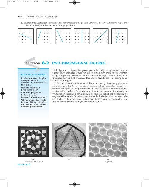
b. On each of the Geoboards below, make a line perpendicular to the given line. Develop, describe, and justify a rule or procedure<br />
for making sure that the two lines are perpendicular.<br />
<strong>SECTION</strong> <strong>8.2</strong> <strong>TWO</strong>-<strong>DIMENSIONAL</strong> <strong>FIGURES</strong><br />
WHAT DO YOU THINK?<br />
• In what ways are triangles<br />
and quadrilaterals<br />
different? In what ways are<br />
they alike?<br />
• How are circles and<br />
polygons related?<br />
• Can every polygon be<br />
broken down into<br />
triangles? Why or why not?<br />
• Why do we use two words<br />
to name different triangles,<br />
but only one word to name<br />
different quadrilaterals?<br />
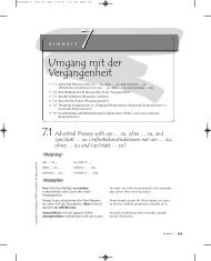
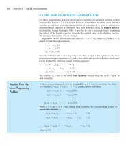
Think of geometric figures that people generally find pleasing, such as those in<br />
Figure 8.45. What words would you use to explain why these objects are interesting<br />
or appealing? When you look at the various objects and pictures, what<br />
similarities do you see between certain objects and shapes—for example, triangles<br />
and hexagons?<br />
When we discuss similarities and differences in my class, many geometric<br />
terms emerge in the discussion. Some students talk about similar shapes—for<br />
example, hexagons in honeycombs and snowflakes, squares in some pictures,<br />
and triangles in others. Some students observe that many of the shapes are<br />
symmetric. In explaining similarities, some students talk about the angles, the<br />
length of sides, or the fact that some figures look similar. Many students observe<br />
that even the more complex shapes can be seen as being constructed from<br />
simpler shapes, such as triangles and quadrilaterals.<br />
(a) (b) (c)<br />
Carpenter’s Wheel quilt Honeycomb<br />
FIGURE 8.45
304150_ch_08_02.qxd 1/16/04 6:06 AM Page 509<br />
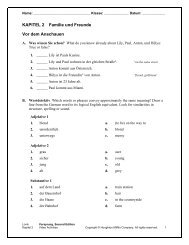
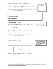
(d)<br />
lamp post<br />
FIGURE 8.45 (continued)<br />
(e)<br />
snowflake<br />
In a few moments, you will begin a systematic exploration of geometric<br />
shapes. Before you do, let us examine a very important framework for understanding<br />
the development of children’s geometric thinking. This model was developed<br />
by Pierre and Dina van Hiele-Geldorf in the late 1950s and is widely<br />
used today. Essentially, the van Hieles found that there are levels, or stages, in<br />
the development of a person’s understanding of geometry. 2<br />
Level 1: Reasoning by resemblance<br />
At this level, the person’s descriptions of, and reasoning about, shapes is<br />
guided by the overall appearance of a shape and by everyday, nonmathematical<br />
language. For example, “This is a square because it looks like one.” Students<br />
at this level may be made aware of the various properties of geometric objects (for<br />
example, that a square has four equal sides), but such awareness can be overridden<br />
by other factors. For example, if we turn a square on its side, the student may insist<br />
that it is no longer a square but now is a diamond.<br />
Level 2: Reasoning by attributes<br />
Section <strong>8.2</strong> / Two-Dimensional Figures 509<br />
(f)<br />
Native American basket weaves<br />
Source: LeRoy Appleton, American Indian Design<br />
and Decoration (New York: Dover, 1950).<br />
At this level, the person can go beyond mere appearance and recognize and describe<br />
shapes by their attributes. A student at this level, seeing the figure above,<br />
can easily classify it as a quadrilateral because it has four sides. However, a student<br />
at this level does not regularly look at relationships between figures. A student<br />
who argues that a figure “is not a rectangle because it is a square” is<br />
reasoning at this level.<br />
2 My writing of this section has been informed by Thomas Fox’s “Implications of Research on<br />
Children’s Understanding of Geometry” in the May 2000 issue of Teaching Children Mathematics,<br />
pp. 572–576.
304150_ch_08_02.qxd 1/16/04 6:06 AM Page 510<br />
510 CHAPTER 8 / Geometry as Shape<br />
INVESTIGATION<br />
8.5<br />
FIGURE 8.46<br />
8.7<br />
Level 3: Reasoning by properties<br />
At this level, the student sees the many attributes of shapes and the relationships<br />
between and among shapes. A student at this level can see that the square<br />
and rhombus have many properties in common, such as opposite sides parallel,<br />
all four sides congruent, and diagonals that bisect each other and are perpendicular.<br />
This enables the student to understand that a square is simply a<br />
rhombus with one additional property—all the angles are right angles.<br />
Level 4: Formal reasoning<br />
Students at this level can understand and appreciate the need to be more systematic<br />
in their thinking. When solving a problem or justifying their reasoning,<br />
they are able to focus on mathematical structures.<br />
The investigations in the text and the accompanying explorations have<br />
been designed to be consistent with this approach. Accordingly, as you are<br />
working in this chapter, reflect on your own thinking. Are you looking at the<br />
problem only on a vague, general level? Are you fixated on just one attribute?<br />
Are you seeing relationships among triangles, among quadrilaterals? As you<br />
move from what to why, are you able to move from solving a problem by random<br />
trial and error to being more systematic and careful in your approach?<br />
With this model in mind, let us begin our exploration of shapes with an investigation<br />
my students have found to be both fun and powerful. Even more<br />
important than knowing the names of all these different shapes will be knowing<br />
their properties and the relationships between and among the shapes. It<br />
is this knowledge that is used by artists, engineers, scientists, and all sorts of<br />
other people.<br />
Recreating Shapes from Memory<br />
For this investigation, you will want to have a pencil and an eraser.<br />
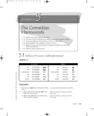
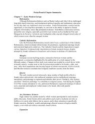
A. Look at Figure 8.46 for about 1 second. Then close the book and draw<br />
Figure 8.46 from memory.<br />
Check the picture again for 1 second. If your drawing was<br />
incomplete or inaccurate, change your drawing so that it is accurate.<br />
Check the picture again for 1 second. Keep doing this until your drawing<br />
is complete and accurate.<br />
Now go back and try to describe your thinking processes as you tried<br />
to re-create the figure. From an information processing perspective, your<br />
eyes did not simply receive the image from the paper; your knowledge<br />
of geometry helped determine how you saw the picture. What did you<br />
hear yourself saying to help you remember the picture? Then read<br />
on. . . .<br />
DISCUSSION<br />
Some students see a diamond and 4 right triangles. Other students see a large<br />
square in which the midpoints of the sides have been connected to make a new<br />
square inside the first square. Yet other students see four right triangles that<br />
have been connected by “flipping” or rotating them.
304150_ch_08_02.qxd 1/16/04 6:06 AM Page 511<br />
FIGURE 8.47<br />
FIGURE 8.48<br />
FIGURE 8.49<br />
FIGURE 8.50<br />
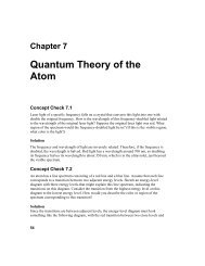
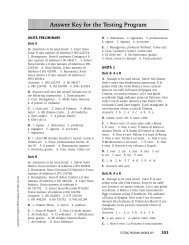
B. Now look at Figure 8.47 for several seconds. Then close the book and try<br />
to draw it from memory. As before, check the picture again for a few<br />
seconds. If your drawing was incomplete or inaccurate, fix it. Keep doing<br />
this until your drawing is complete and accurate. Then go back and<br />
describe the thinking processes you engaged in as you tried to re-create<br />
the figure. . . .<br />
DISCUSSION<br />
Section <strong>8.2</strong> / Two-Dimensional Figures 511<br />
This figure was more complex. Some students see a whole design and try to remember<br />
it.<br />
Some decompose the design into four black triangles and four rectangles as<br />
shown in Figure 8.48.<br />
The figure can also be seen as being composed of 9 squares, which can also<br />
be seen in Figure 8.48. The four corner squares have been cut to make congruent<br />
right triangles. Each of the other four squares on the border has been cut<br />
into two congruent rectangles.<br />
Some students re-created this figure by seeing a whole square and then<br />
looking at what was cut out (see Figure 8.49). That is, they saw that they needed<br />
to cut out each corner, and they saw that they needed to cut out a rectangle<br />
on the middle of each side. Finally, they remembered to cut out a square in the<br />
center.<br />
When I did this exercise myself, I saw a “square race track” with a similar<br />
pattern on each corner (Figure 8.50).<br />
This is a famous quilting pattern called the Churn Dash. When people<br />
made their own butter, the cream was poured into a pail called a churn. Then<br />
the churner rolled a special pole back and forth with his or her hands. At the<br />
end of the pole was a wooden piece called a dash, which was shaped like the<br />
figure you saw. If you make many copies of this pattern and put them together,<br />
you can see what a Churn Dash quilt looks like.<br />
There are several implications for teaching from this investigation. How a<br />
person re-creates the figure is related to the person’s spatial-thinking preferences<br />
and abilities. Different people “see” different objects. That is, not everyone<br />
sees the figure in the same way. Although there are differences in how<br />
people re-create the figure, very few people can re-create the figure without<br />
doing some kind of decomposing—that is, without breaking the shape into<br />
smaller parts. Being able to do this depends partly on spatial skills and partly<br />
on being able to use various geometric ideas (congruent, triangle, square, rectangle)<br />
at least at an intuitive level.<br />
Although some people manage to live happy, productive lives at the lowest<br />
van Hiele level, an understanding of basic geometric figures and the relationships<br />
among them is often helpful in everyday life (for example, in home<br />
repair projects and quilting) and in many occupations. Now that your interest<br />
in geometric figures has been piqued by this investigation and the pictures at<br />
the beginning of the section, let us examine the characteristics and properties of<br />
basic geometric shapes.<br />
Before we examine specific kinds of polygons, beginning with triangles, the<br />
following investigation will serve to “open your thinking”—to get you to look<br />
at polygons not only through the zoom lens, which reveals specific properties
304150_ch_08_02.qxd 1/16/04 6:06 AM Page 512<br />
512 CHAPTER 8 / Geometry as Shape<br />
INVESTIGATION<br />
8.6<br />
and definitions, but also through the wide-angle lens, in which you see all the<br />
attributes. For example, a person is not just a person. She might be a mother, a<br />
sister, a daughter, a scientist, a Democrat, and so on. Should you become a<br />
friend of this person, you come to know her many facets. Similarly, if you become<br />
a “friend” of shapes, you come to know the many “sides” of the shapes<br />
with which you are working.<br />
Look at the polygons in<br />
Figure 8.51. Think of all the<br />
attributes, all the characteristics,<br />
anything about the polygons<br />
that might be important to state<br />
or measure. Write down your<br />
list before reading on. . . .<br />
DISCUSSION<br />
All the Attributes<br />
FIGURE 8.51<br />
As you compare the following lists to yours, read actively. If you made the<br />
same observation, did you use the same wording? If not, do you understand<br />
the wording here? If you missed one of these attributes, why? Do you understand<br />
it now? Are there other attributes that you noticed?<br />
First figure Second figure<br />
6 sides 6 sides<br />
Top and bottom sides parallel to each other Top and bottom sides parallel to each other<br />
All three pairs of opposite sides parallel<br />
Concave Convex<br />
2 sets of congruent sides 4 congruent sides; the other pair is also congruent<br />
2 acute angles, 2 right angles, 2 reflex angles 4 obtuse angles, 2 right angles<br />
3 pairs of congruent angles Opposite angles congruent<br />
1 line of reflection symmetry No reflection symmetry<br />
No rotation symmetry 12-turn<br />
rotation symmetry<br />
Does not tessellate Tessellates<br />
A key idea here is to realize that there are lots of attributes and that knowing<br />
these attributes and combinations of attributes of a shape helps chemists<br />
and physicists to understand the behavior of a molecule or shape; helps<br />
builders to know which shapes work together better either in terms of structure<br />
and strength or in terms of appearance; and helps artists and designers to make<br />
designs that are the most appealing. As you read on, think of multiple attributes<br />
and of attributes that different objects have in common.
304150_ch_08_02.qxd 1/16/04 6:06 AM Page 513<br />
INVESTIGATION<br />
8.7<br />
■ Language ■<br />
8.8<br />
What other words might you<br />
use to describe the<br />
intersecting and not<br />
intersecting subsets?<br />
Some students use the<br />
phrase “trace over,” and others<br />
talk about figures that “run<br />
over themselves” or “cross<br />
themselves.” Other students<br />
talk about the set of figures<br />
that contain two smaller<br />
regions within each figure.<br />
Classifying Figures<br />
Before we examine and classify important two-dimensional shapes, we first<br />
need to investigate the kinds of possible two-dimensional shapes. Although<br />
most of elementary students’ exploration of two-dimensional figures will<br />
involve polygons and circles, it is important to know that these figures<br />
represent just a small subset of the kinds of figures that mathematicians<br />
study. Both circles and polygons are curves. A mathematical curve can be<br />
thought of as a set of points that you can trace without lifting your pen or<br />
pencil. If you watch young children making drawings, you discover that they<br />
make all sorts of curves!<br />
As you might expect, if we look at any set of curves, there are many<br />
ways to classify them. As I have done throughout this book, rather than<br />
giving you the major classifications, I will engage you in some thinking<br />
before presenting them. Look at the 13 shapes in Figure 8.52 and classify<br />
them into two or more groups so that each group has a common<br />
characteristic. Do this in as many different ways as you can, and then<br />
read on. . . .<br />
1 2 3 4 5 6 7<br />
8 9 10 11 12 13<br />
FIGURE 8.52<br />
DISCUSSION<br />
One way to sort the figures is shown below. How would you describe the figures<br />
in set A and the figures in set B? Do this before reading on. . . .<br />
Set A<br />
Set B<br />
Section <strong>8.2</strong> / Two-Dimensional Figures 513<br />
The figures in set A are said to be simple curves. We can describe simple<br />
curves in the following way: A figure is a simple curve if we can trace the figure<br />
in such a way that we never touch a point more than once. If you look at<br />
the figures in set A, you can see that they all have this characteristic; and all the<br />
figures in set B have at least one point where the pencil touches twice, no matter<br />
how you trace the curve.
304150_ch_08_02.qxd 1/16/04 6:06 AM Page 514<br />
514 CHAPTER 8 / Geometry as Shape<br />
CLASSROOM CONNECTION<br />
Using the terms developed in<br />
this investigation, how would<br />
you classify dot-to-dot pictures?<br />
Now look at the curves in sets C and D. How would you describe the figures<br />
in set C and the figures in set D? Do this before reading on. . . .<br />
Set C<br />
Set D<br />
The figures in set C are said to be closed curves. We can describe closed<br />
curves in the following way: A figure is a closed curve if we can trace the figure<br />
in such a way that our starting point and our ending point are the same. If<br />
you look at the figures in set C, you can see that they all have this characteristic;<br />
and no matter how you try, you cannot trace the figures in set D with the<br />
same starting and ending point.<br />
Now look at the curves in sets E, F, and G. How would you describe the figures<br />
in set E, the figures in set F, and the figures in set G? Do this before reading<br />
on. . . .<br />
Set E<br />
Set F<br />
Set G<br />
These three sets are interesting for two reasons. First, these sets are likely to<br />
be generated in the classroom—both your classroom and the elementary classroom.<br />
Second, the language used to describe the three sets poses a challenge,<br />
for most people describe the figures in set E as consisting only of curvy lines,<br />
the figures in set F as consisting only of straight line segments, and the figure<br />
in set G as having both curvy and straight line segments. The challenge here is<br />
that when mathematicians use the word curve, this word encompasses both<br />
curvy and straight line segments—a curve is a set of points that you can trace<br />
without lifting your pen or pencil. There is nothing wrong with students’ use<br />
of the terms curvy and straight. What is important is the realization that we are<br />
using the words curve and curvy in different ways. We do this all the time in<br />
everyday English. Recall the various uses of the word hot in Chapter 1: ”It sure<br />
is a hot day.” “I love Thai food because it is hot.” “This movie is really hot!”<br />
Most of our investigations of curves will focus on simple closed curves.<br />
Looking at the descriptions above, try to define the term simple closed curve before<br />
reading on. . . .<br />
We will define a simple closed curve as a curve that we can trace without<br />
going over any point more than once while beginning and ending at the same<br />
point. The set of polygons is one small subset of the set of simple closed curves.<br />
At this point, you might want to do the following activity with another<br />
student.<br />
• Draw a simple closed curve.<br />
• Draw a simple open curve.
304150_ch_08_02.qxd 1/16/04 6:06 AM Page 515<br />
■ History ■<br />
Generally, when a theorem<br />
is named after a person, it<br />
is named after the person<br />
who first proved the theorem.<br />
In this case, Jordan’s proof<br />
was found to be incorrect, but<br />
the theorem is still named<br />
after him!<br />
• Draw a nonsimple closed curve.<br />
• Draw a nonsimple open curve.<br />
Exchange figures with another student. Do you both agree that each of the<br />
other’s drawings matches the description? If so, move on. If not, take some time<br />
to discuss your differences.<br />
There is an important mathematical theorem known as the Jordan curve<br />
theorem, after Camille Jordan: Any simple closed curve partitions the plane into<br />
three disjoint regions: the curve itself, the interior of the curve, and the exterior<br />
of the curve. See the examples in Figure 8.53.<br />
Exterior<br />
Interior<br />
FIGURE 8.53<br />
I know that many students’ reaction to this theorem is “Why do we need to<br />
prove something that is so obvious?” As mentioned before, being critical (“to<br />
examine closely”) is an attitude that I invite. In the examples in Figure 8.53, deciding<br />
whether a point is inside or outside is easy. However, look at Figure 8.54.<br />
Although this figure is a simple closed curve, it is a rather complicated figure,<br />
and such complicated shapes are encountered in some fields of science. Is<br />
point A inside or outside? How would you determine this? Think before reading<br />
on. . . .<br />
FIGURE 8.54<br />
Section <strong>8.2</strong> / Two-Dimensional Figures 515<br />
A<br />
Exterior<br />
Interior<br />
(a) (b)<br />
Some wag once remarked that mathematicians are among the laziest<br />
people on earth because they are always looking for shortcuts and simpler<br />
ways to solve problems. Thus you may be wondering whether someone has
304150_ch_08_02.qxd 1/16/04 6:06 AM Page 516<br />
516 CHAPTER 8 / Geometry as Shape<br />
CLASSROOM CONNECTION<br />
The active and curious reader<br />
here might realize that this<br />
procedure might have<br />
applications for solving mazes,<br />
and there is a branch of<br />
mathematics that does analyze<br />
mazes. Another active and<br />
curious reader might realize<br />
and/or remember that most<br />
children enjoy the challenge of<br />
solving mazes.<br />
TABLE <strong>8.2</strong><br />
Number<br />
of sides Name<br />
3 sides Triangle<br />
4 sides Quadrilateral<br />
5 sides Pentagon<br />
6 sides Hexagon<br />
7 sides Heptagon<br />
8 sides Octagon<br />
n sides n-gon<br />
8.9<br />
found an easier way to solve these problems. Indeed, someone has. I can use<br />
the shape in Figure 8.55 to illustrate the method. Start at a point that is clearly<br />
outside the shape and draw a line segment connecting that point to the point<br />
you are looking at; it helps if you pick an outside point so that the line segment<br />
will cross the curve in as few points as possible. Each time you cross a point,<br />
it’s like a gate—if you were outside, you are now inside; if you were inside, you<br />
are now outside. Thus it is a relatively simple matter to determine that point B<br />
is inside the curve.<br />
FIGURE 8.55<br />
Now go back to the first shape to see whether point A is inside or outside.<br />
As an active reader you will want to work on the figure to verify to your satisfaction<br />
that the method just described really does work.<br />
Polygons<br />
We are now ready to begin our exploration of polygons, which can be defined<br />
as simple closed curves composed only of line segments. Thus the simple<br />
closed curve in Figure 8.53(a) is not a polygon, whereas the simple closed curve<br />
in Figure 8.53(b) (which looks like the state of Nevada) is a polygon. On any<br />
polygon, the point at which two sides meet is called a vertex, the plural of<br />
which is vertices. The line segments that make up the polygon are called sides.<br />
The word polygon has Greek origins: poly-, meaning “many,” and -gon,<br />
meaning “sides.” You are already familiar with many kinds of polygons. Just as<br />
we found in Chapter 2 that the names we give numbers have an interesting history,<br />
so do the names we give to polygons. The most basic naming classification<br />
involves the number of sides (see Table <strong>8.2</strong>).<br />
Now that we have a good general definition of the term polygon, we can<br />
spend time examining triangles, quadrilaterals, and a few specific kinds of<br />
polygons.<br />
Triangles<br />
B<br />
Triangles are found in every aspect of our lives—in buildings, in art, in science<br />
(see Figures 8.56 and 8.57). They are truly “building-block” shapes. Every bicycle<br />
I have seen has triangles. Bridges will always contain triangles. If you
304150_ch_08_02.qxd 1/16/04 6:06 AM Page 517<br />
INVESTIGATION<br />
8.8<br />
look at the skeleton of buildings, and the scaffolding around the building, you<br />
will always see triangles. Why? Rather than give you the answer, we will use<br />
the next investigation to think about this question.<br />
FIGURE 8.56 FIGURE 8.57<br />
Why Triangles Are So Important<br />
Cut some strips of paper from a file folder or other stiff material. Punch a<br />
hole in the ends and use paper fasteners (improvise if you need to; for<br />
instance, you can use paper clips). Make one triangle and one quadrilateral,<br />
as shown in Figure 8.58. It need not be an equilateral triangle or a square.<br />
What do you see? . . .<br />
DISCUSSION<br />
FIGURE 8.58<br />
Section <strong>8.2</strong> / Two-Dimensional Figures 517<br />
As you saw, the triangle won’t move—we call it a rigid structure. However, the<br />
quadrilateral does move; it is not stable. Make another strip and connect two<br />
nonadjacent vertices of your quadrilateral. What happens now? It will remain<br />
in the shape. If it is a square, it will remain a square; if it is a parallelogram, it<br />
will remain a parallelogram. This is because the addition of that diagonal actually<br />
created two triangles, which, as you have found, are rigid structures. The<br />
next time you walk about campus and about town, look for triangles. You will<br />
suddenly see them everywhere!<br />
As you already know, there are many kinds of triangles. A crucial goal of<br />
the next investigation is for your own understanding of triangles to become<br />
more powerful. Thus, as always, please do the investigation, rather than just<br />
reading through it quickly because “I already know this stuff.”
304150_ch_08_02.qxd 1/16/04 6:06 AM Page 518<br />
518 CHAPTER 8 / Geometry as Shape<br />
INVESTIGATION<br />
8.9<br />
Classifying Triangles<br />
You will find nine triangles in Figure 8.59. Copy them and cut them out, and<br />
then separate them into two or more subsets so that the members of each<br />
subset share a characteristic in common. Can you come up with a name for<br />
each subset? What names might children give to different subsets? Do this in<br />
as many different ways as you can before reading on. . . .<br />
FIGURE 8.59<br />
DISCUSSION<br />
STRATEGY 1: Consider sides<br />
One way to classify triangles is by the length of their sides: all three sides having<br />
equal length, two sides having equal length, no sides having equal length.<br />
There are special names for these three kinds of triangles.<br />
• If all three sides have the same length, then we say that the triangle is<br />
equilateral.<br />
• If at least two sides have the same length, then we say that the triangle is<br />
isosceles.<br />
• If all three sides have different lengths—that is, no two sides have the same<br />
length—then we say that the triangle is scalene.<br />
Which of the triangles in Figure 8.59 are scalene? Which are isosceles?<br />
Which are equilateral?<br />
STRATEGY 2: Consider angles<br />
We can also classify triangles by the relative size of the angles—that is, whether<br />
they are right, acute, or obtuse angles. This leads to three kinds of triangles:<br />
right triangles, obtuse triangles, and acute triangles.<br />
• We define a right triangle as a triangle that has one right angle.<br />
• We define an obtuse triangle as a triangle that has one obtuse angle.<br />
• We define an acute triangle as a triangle that has three acute angles.<br />
Many students see a pattern: A right triangle has one right angle, an obtuse<br />
triangle has one obtuse angle, yet an acute triangle has three acute angles. What<br />
was the pattern? Why doesn’t it hold? Think before reading on. . . .
304150_ch_08_02.qxd 1/16/04 6:06 AM Page 519<br />
FIGURE 8.60<br />
■ Mathematics ■<br />
Did you notice the geometric<br />
balance in Figure 8.61, which<br />
represents the Cartesian<br />
product of the two sets of<br />
triangles?<br />
CLASSROOM CONNECTION<br />
Some students have told me<br />
that this investigation is huge<br />
for them, because they had<br />
never thought about<br />
organization and classification<br />
with respect to triangles.<br />
Triangles just were!<br />
The key to this comes from looking at the triangles from a different perspective:<br />
Every right triangle has exactly two acute angles, and every obtuse triangle<br />
has exactly two acute angles; thus a triangle having more than two acute<br />
angles will be a different kind of triangle. This perspective is represented in<br />
Table 8.3. Does it help you to understand better the three definitions given above?<br />
TABLE 8.3<br />
STRATEGY 3: Consider angles and sides<br />
This naming of triangles goes even further. What name would you give to the<br />
triangle in Figure 8.60?<br />
This triangle is both a right triangle and an isosceles triangle, and thus it is<br />
called a right isosceles triangle or an isosceles right triangle. How many possible<br />
combinations are there, using both classification systems? Work on this<br />
before reading on. . . .<br />
There are many strategies for answering this question. First of all, we find<br />
that there are nine possible combinations (see Figure 8.61). We can use the idea<br />
of Cartesian product to determine all nine. That is, if set S represents triangles<br />
classified by side, S {Equilateral, Isosceles, Scalene}, and set A represents triangles<br />
classified by angle, A {Acute, Right, Obtuse}, then S A represents<br />
the nine possible combinations.<br />
FIGURE 8.61<br />
However, not all nine combinations are possible. For example, any equilateral<br />
triangle must also be an acute triangle. (Why is this?) Therefore, “equilateral<br />
acute” is a redundant combination. However, it is possible to have scalene<br />
triangles that are acute, right, and obtuse. Similarly, we can have isosceles triangles<br />
that are acute, right, and obtuse.<br />
Name the two triangles in Figure 8.62. Then read on. . . .<br />
FIGURE 8.62<br />
Equilateral<br />
Isosceles<br />
Scalene<br />
Section <strong>8.2</strong> / Two-Dimensional Figures 519<br />
First angle Second angle Third angle Name of triangle<br />
Acute Acute Right Right triangle<br />
Acute Acute Obtuse Obtuse triangle<br />
Acute Acute Acute Acute triangle<br />
Acute<br />
Right<br />
Obtuse
304150_ch_08_02.qxd 1/16/04 6:06 AM Page 520<br />
520 CHAPTER 8 / Geometry as Shape<br />
INVESTIGATION<br />
8.10<br />
8.10<br />
Both are obtuse, isosceles triangles. The orientation on the left is the standard<br />
orientation for isosceles triangles. Any time we position a triangle so that<br />
one side is horizontal, we call that side the base. As stated at the beginning of<br />
this chapter, students often see only one aspect of a triangle; for example, they<br />
see the triangle at the left as isosceles but not also obtuse, and they see the triangle<br />
at the right as obtuse but not also isosceles.<br />
CLASSROOM CONNECTION<br />
Children’s development of triangles is fascinating. In several studies, children were<br />
given many shapes and asked to identify the shapes. Young children tend to<br />
identify the equilateral triangle in the “standard” position (base parallel to the<br />
bottom of the page) as a “true” triangle. They will often reject triangles such as the<br />
ones below because they are too pointy or turned upside down. Recall level 1 in<br />
the van Hiele model. One of my all-time favorite examples occurred when a firstgrader<br />
was given the pattern shown in Figure 8.63 and was asked to continue the<br />
FIGURE 8.63<br />
pattern. After studying the pattern, she said, “Triangle, triangle, wrong triangle,<br />
triangle, triangle, wrong triangle, triangle. . . . The next shape is a right triangle!” 3 It<br />
is important to note that this child was doing wonderful thinking—she was seeing<br />
patterns, and she was looking at attributes, and she was at the beginning of her<br />
understanding of triangles.<br />
As mentioned earlier, one of the new NCTM process standards is representation.<br />
As I have also mentioned earlier, one definition of understanding has to<br />
do with the quantity and quality of connections the learner can make within<br />
and between various ideas. In this case, a new representation of the relationship<br />
between and among triangles will help to deepen your understanding.<br />
More of these problems can be found in Exploration 8.13. These diagrams are<br />
also being used more and more in elementary schools because of their tremendous<br />
potential to help children see more relationships and connections.<br />
Triangles and Venn Diagrams<br />
Recall our work with Venn diagrams in Chapter 2. Venn diagrams can help<br />
us to understand how concepts are and are not related. Let us take two<br />
kinds of triangles: right triangles and isosceles triangles. Draw several right<br />
triangles and draw several isosceles triangles. Which of these triangles could<br />
be placed in both categories? That is, which are right triangles and also<br />
3 From “Shape Up!” by Christine Oberdorf and Jennifer Taylor-Cox, published in the February 1999<br />
issue of Teaching Children Mathematics, pp. 340–345.
304150_ch_08_02.qxd 1/16/04 6:06 AM Page 521<br />
■ Mathematics ■<br />
Interestingly, all right isosceles<br />
triangles have the same shape.<br />
That is, if you found the ratio<br />
of lengths of the sides of two<br />
right isosceles triangles,<br />
converted this to a percent,<br />
placed the larger one on a<br />
copy machine, and entered<br />
that percent in the reduction<br />
button, the smaller triangle<br />
would come out. We will<br />
explore this notion of<br />
similarity in Section 9.3.<br />
isosceles triangles? Make a Venn diagram that illustrates the relationships<br />
between the right and isosceles triangles, and place each triangle in the<br />
appropriate region of the diagram.<br />
Now draw several acute triangles and draw several equilateral triangles.<br />
Which of these triangles could be placed in both categories? How are these<br />
triangles related to each other? Make a Venn diagram that illustrates the<br />
relationships between the acute and equilateral triangles, and place each<br />
triangle in the appropriate region of the diagram.<br />
DISCUSSION<br />
When we have two groups of objects and look at how they are related, there are<br />
three possible relationships. They may be disjoint—each object is in one or the<br />
other group; there may be overlap—some objects are in both groups; or one<br />
group may be a subset of the other. Each of these relationships (remember the<br />
van Hiele levels) is represented with a different diagram, as shown in Figure 8.64.<br />
FIGURE 8.64<br />
Look at your Venn diagrams and think of what you just read. Do you want<br />
to change your diagrams? If you couldn’t make the Venn diagrams because you<br />
just didn’t understand the question, can you do so now? Do this before reading<br />
on. . . .<br />
Because some triangles are both right and isosceles, those triangles can be<br />
placed in the center, showing that they belong to both sets (see Figure 8.65). Because<br />
equilateral triangles can contain only acute angles, all equilateral triangles<br />
are acute triangles. Hence the equilateral triangles are in a ring that is<br />
inside the ring that represents acute triangles.<br />
FIGURE 8.65<br />
Right ∆<br />
Isosceles ∆<br />
Section <strong>8.2</strong> / Two-Dimensional Figures 521<br />
Acute ∆<br />
Equilateral ∆
304150_ch_08_02.qxd 1/16/04 6:06 AM Page 522<br />
522 CHAPTER 8 / Geometry as Shape<br />
FIGURE 8.66<br />
Triangle Properties<br />
You probably remember that the sum of the measures of the angles in any<br />
triangle is 180 degrees. How could you convince someone who does not<br />
know that?<br />
This is a case in which the van Hiele levels are instructive. A level 2 activity<br />
would be to have the students measure and add the angles in several triangles.<br />
If their measuring was relatively accurate, one or more students would<br />
see the pattern and offer a hypothesis that the sum is always 180.<br />
An example of a level 3 activity, which I recommend if you have never<br />
done it, is to cut off the three corners of a triangle as in Figure 8.66 and then put<br />
the three corners together. What do you see?<br />
An example of a level 4 activity would be a formal proof.<br />
Special Line Segments in Triangles<br />
There are four special line segments that have enjoyed tremendous influence<br />
in Euclidean geometry: angle bisector, median, altitude, and perpendicular<br />
bisector.<br />
A median is a line segment that connects a vertex to the midpoint of the opposite<br />
side.<br />
In triangle SAT (Figure 8.67), TR is a median. Hence SR RA.<br />
T<br />
FIGURE 8.67<br />
An angle bisector is a line segment that bisects an angle of a triangle.<br />
In triangle ABC (Figure 8.68), AD is an angle bisector. Hence, mBAD <br />
mDAC.<br />
A<br />
S<br />
B<br />
FIGURE 8.68<br />
R A<br />
A perpendicular bisector is a line that goes through the midpoint of a side<br />
and is perpendicular to that side. In triangle PEN (Figure 8.69), MX is a per-<br />
i<br />
D<br />
C
304150_ch_08_02.qxd 1/16/04 6:06 AM Page 523<br />
FIGURE 8.71<br />
FIGURE 8.72<br />
pendicular bisector of side PN, because M is the midpoint of PN and MX is perpendicular<br />
to PN.<br />
FIGURE 8.69<br />
An altitude is a perpendicular line segment that connects a vertex to the<br />
side opposite that vertex. In some cases, as in SAT in Figure 8.70, we need to<br />
extend the opposite side to construct the altitude.<br />
In triangle ABC (Figure 8.70), BF is an altitude. Hence, mBFA <br />
mBFC 90.<br />
In triangle STA, TP is an altitude. Hence, mTPA 90.<br />
A<br />
FIGURE 8.70<br />
B<br />
F<br />
P<br />
Section <strong>8.2</strong> / Two-Dimensional Figures 523<br />
E<br />
M<br />
C P<br />
Many students have trouble with the idea of an altitude being outside the<br />
triangle. This happens when we have an obtuse triangle oriented with one side<br />
of the obtuse angle as the base of the triangle. If you are having trouble connecting<br />
the definition of altitude in these situations, I recommend the following:<br />
Trace the triangle and cut it out. Stand it up so that SA is on the plane of your<br />
desk and T is above that plane. Now draw a line from T that goes “straight<br />
down.” What do you notice?<br />
If triangle STA were large enough so that you could stand with your head<br />
at point T, the length of line segment TP would tell you how tall you were!<br />
T<br />
After reading the preceding discussion, a skeptical reader might ask, “So<br />
what? What is the value of these line segments, other than to mathematicians?”<br />
One response is that there is practical value, and another response is that there<br />
are some really cool relationships here. Let me explain.<br />
The segment with the most practical value is the median. The point where<br />
all three medians meet is called the centroid and is the center of gravity of the<br />
triangle (see Figure 8.71). That is, if you found this point, made a copy of the<br />
triangle with wood, and placed the triangle on a nail at that point, the triangle<br />
would balance. Center of gravity is related to balance and is an important concept<br />
in the design of many objects—cars, furniture, and art, to mention just a few.<br />
The point where the three perpendicular bisectors meet is called the circumcenter<br />
(see Figure 8.72). It turns out that this point is equidistant from each<br />
of the three vertices of the triangle. Thus you can draw a circle so that all three<br />
vertices of the triangle lie on the circle and the rest of the triangle is inside the<br />
circle. We say that the circle circumscribes the triangle.<br />
X<br />
S<br />
N<br />
A
304150_ch_08_02.qxd 1/16/04 6:06 AM Page 524<br />
524 CHAPTER 8 / Geometry as Shape<br />
FIGURE 8.73<br />
FIGURE 8.74<br />
8.11<br />
The point where the three angle bisectors meet is called the incenter (see<br />
Figure 8.73). It turns out that this point is equidistant from each of the three<br />
sides of the triangle. Thus you can draw a circle so that the circle touches (is tangent<br />
to) each of the three sides of the triangle; in this case, the circle is inside the<br />
triangle. We say that the circle is inscribed in the triangle.<br />
The point where the three altitudes meet is called the orthocenter (see Figure<br />
8.74). The orthocenter has connections to other geometric ideas. For example,<br />
there is a connection between the construction of a parabola and the<br />
orthocenter of a triangle.<br />
There are two amazing things about these line segments. The first is that in<br />
any triangle there are three medians, three perpendicular bisectors, three angle<br />
bisectors, and three altitudes. In each case, the three line segments will always<br />
meet at a single point—they are concurrent. That is, the three medians will always<br />
meet at one point in any triangle, the three perpendicular bisectors will<br />
always meet at one point in any triangle, and so on. Now, except for the case of<br />
the equilateral triangle, these points are not the same point. In fact, in a scalene<br />
triangle, the four points are all different. However (and this is the other cool<br />
thing), there is a relationship among the centroid, circumcenter, and the orthocenter.<br />
In any triangle, they are collinear! Do you understand this? Figure 8.75<br />
illustrates this fact, which Leonard Euler first discovered. We even call the line<br />
containing these three points an Euler line. If you are curious, you can type in<br />
these terms on a search engine. You will even find websites that have interactive<br />
features allowing you to see the situations where these four points are distinct<br />
but collinear and the situations where they converge into one point.<br />
Congruence<br />
C<br />
A<br />
B<br />
FIGURE 8.75<br />
A - centroid<br />
B - circumcenter<br />
C - orthocenter<br />
As you have seen from your geometry explorations, questions sometimes arise<br />
about whether two figures are “the same” or not. Such observations and questions<br />
deal with the idea of congruence.<br />
At an informal level, we can say that two figures are congruent if and only<br />
if they have the same shape and size. An informal test of congruence is to see<br />
whether you can superimpose one figure on top of the other. This is closely connected<br />
to how children initially encounter the concept and is related to the dictionary<br />
definition: “coinciding exactly when superimposed.” 4 That is, if one<br />
figure can be superimposed over another so that it fits perfectly, then the two<br />
figures are congruent.<br />
Formally, we say that two polygons are congruent if and only if all pairs of<br />
corresponding parts are congruent. In other words, in order for us to conclude<br />
that two polygons are congruent, two conditions have to be met: (1) Each corresponding<br />
pair of angles have the same measure and (2) each corresponding<br />
pair of sides have the same length. We use the symbol to denote congruence.<br />
For example, in Figure 8.76, triangle CAT and triangle DOG are congruent<br />
iff C D, A O, T G, CA DO, AT OG, and TC GD.<br />
4 Copyright © 1996 by Houghton Mifflin Company. Reproduced by permission from The American<br />
Heritage Dictionary of the English Language, Third Edition.
304150_ch_08_02.qxd 1/16/04 6:06 AM Page 525<br />
INVESTIGATION<br />
8.11<br />
C<br />
A<br />
FIGURE 8.76<br />
Section <strong>8.2</strong> / Two-Dimensional Figures 525<br />
T D<br />
The notions of congruent and equal are related concepts. We use the term<br />
congruence when referring to having the same shape, and we use the term equal<br />
when referring to having the same numerical value. Thus we do not say that<br />
two triangles are equal; we say that they are congruent. Similarly, when we<br />
look at line segments and angles of polygons, we speak of congruent line segments<br />
and congruent angles. However, when we look at the numerical value of<br />
the line segments and angles, we say that the lengths of two line segments are<br />
equal and that the measures of two angles are equal.<br />
Congruence is a big idea, both in geometry and beyond the walls of the<br />
classroom. Many important properties and relationships come from exploring<br />
congruence. The following investigations (and the related explorations) will<br />
help move your understanding of congruence to higher van Hiele levels, from<br />
the “can fit on top,” geometric reasoning by resemblance, to understanding that<br />
all corresponding parts are congruent, to geometric reasoning by attributes, to<br />
geometric reasoning by properties, which we shall examine now.<br />
■ Outside the Classroom ■<br />
When do we need congruence in everyday life or in work situations? Take a few<br />
minutes to think about this before reading on. . . .<br />
Congruence is important in manufacturing; for example, the success of<br />
assembly-line production depends on being able to produce parts that are<br />
congruent. Henry Ford changed our world by conceiving of making cars not one<br />
at a time but as many sets of congruent parts. For example, the left front fender of<br />
a 2003 Dodge Caravan is congruent to the left front fender of any other 2003<br />
Dodge Caravan. One of the differences between a decent quilt and an excellent<br />
one is being able to ensure that all the squares are congruent. This is quite<br />
difficult when using complex designs. Most of the manipulatives teachers use with<br />
schoolchildren (Pattern Blocks, unifix cubes, Cuisenaire rods, and fraction bars)<br />
have congruent sets of pieces.<br />
Congruence with Triangles<br />
For this you need a protractor and a compass, although you can improvise<br />
without them. Do both questions on a blank sheet of paper. First, see how<br />
many different triangles you can make that have the following attributes:<br />
The base is 50 millimeters (mm). The angle coming from the left side of the<br />
base is 30°, and the side coming from the left side of the base is 30 mm.<br />
Second, see how many different triangles you can make that have the<br />
following attributes: The base is 30 mm. The angle coming from the left side<br />
of the base is 30°, and the side coming from the right side of the base is<br />
25 mm. Do this before reading on. . . .<br />
O<br />
G
304150_ch_08_02.qxd 1/16/04 6:06 AM Page 526<br />
526 CHAPTER 8 / Geometry as Shape<br />
■ Language ■<br />
Some books define a trapezoid<br />
as having exactly one pair of<br />
parallel sides. I have spoken<br />
with many mathematicians<br />
about this particular<br />
definition—some prefer the<br />
definition used here and some<br />
prefer the other one. There is<br />
no right answer, but rather<br />
reasons behind each one.<br />
There are two reasons why I<br />
use the definition given here.<br />
First, I would find it odd to<br />
define an isosceles triangle as<br />
having at least two congruent<br />
sides but then a trapezoid as<br />
having exactly one set of<br />
parallel sides. If we are going<br />
to say a trapezoid has exactly<br />
one pair of parallel sides, then<br />
an isosceles triangle should<br />
have exactly two congruent<br />
sides. There are reasons why<br />
isosceles is defined the way it<br />
is, reasons beyond the scope<br />
of this book, but I am<br />
persuaded by parallel usage<br />
here. Second, defining<br />
trapezoid this way enables us<br />
to represent relationships<br />
among quadrilaterals in a<br />
more elegant way.<br />
DISCUSSION<br />
There is only one triangle that can be drawn in the first case. However, in the<br />
second case, there are two possible triangles. Thus there is not enough information<br />
about the triangle to specify exactly one triangle (see Figure 8.77).<br />
30 mm<br />
30° 30°<br />
FIGURE 8.77<br />
In Section 8.1, we said that two points determine a line; here, we are looking<br />
at what determines a triangle. This notion of determining or specifying is important<br />
in mathematics, both for congruence (When are two figures congruent?)<br />
and for definitions (How much do we need to specify to determine a shape?)<br />
For example, we can define a rectangle as a quadrilateral with four equal<br />
angles. Now a rectangle has many more properties than four congruent angles.<br />
However, mathematicians have discovered that this information—quadrilateral,<br />
four congruent angles—is sufficient so that only rectangles can be drawn<br />
that meet that criteria. Thus the notion of “determines” is an important one<br />
in mathematics. In elementary school we do not get terribly technical, but that<br />
is not the same as saying we just have fun and play around. When we ask<br />
children to explore well-focused questions, their understanding of shapes and<br />
relationships between and among shapes and their ability to see and apply<br />
properties can grow tremendously. When this happens, high school mathematics<br />
makes much more sense!<br />
Quadrilaterals<br />
50 mm A B<br />
We found that we could describe different kinds of triangles by looking at their<br />
angles or by looking at relationships among their sides. With quadrilaterals,<br />
which have one more side, new possibilities for categorization emerge: parallel<br />
sides, adjacent vs. opposite sides, relationships between diagonals, and the notion<br />
of concave and convex. Thus, how we go about naming and classifying<br />
quadrilaterals is not the same as how we name and classify triangles.<br />
In this book, we will define the following kinds of quadrilaterals:<br />
• A trapezoid (Figure 8.78) is defined<br />
as a quadrilateral with at least one<br />
pair of parallel sides.<br />
• A parallelogram (Figure 8.79) is<br />
defined as a quadrilateral in which<br />
both pairs of opposite sides are<br />
parallel.<br />
• A kite (Figure 8.80) is defined as a<br />
quadrilateral in which two pairs of<br />
adjacent sides are congruent.<br />
C<br />
FIGURE 8.78<br />
FIGURE 8.79<br />
FIGURE 8.80<br />
D
304150_ch_08_02.qxd 1/16/04 6:06 AM Page 527<br />
■ Outside the<br />
Classroom ■<br />
How many of each kind of<br />
quadrilateral can you find in<br />
everyday life?<br />
• A rhombus (Figure 8.81) is defined<br />
as a quadrilateral in which all sides<br />
are congruent.<br />
• A rectangle (Figure 8.82) is defined<br />
as a quadrilateral in which all<br />
angles are congruent.<br />
• A square (Figure 8.83) is defined as<br />
a quadrilateral in which all four<br />
sides are congruent and all four<br />
angles are congruent.<br />
An active reader may have noted that there are many other possible categories<br />
of quadrilaterals. For example, there are many different quadrilaterals<br />
that have at least one right angle or exactly three congruent sides. Just as we<br />
called the triangle with no sides congruent a scalene triangle, we could call a<br />
quadrilateral with no sides congruent a scalene quadrilateral. If we have names<br />
for quadrilaterals with two pairs of adjacent sides congruent and quadrilaterals<br />
with two pair of opposite sides congruent, why stop there? The primary reason<br />
why we have names for the quadrilaterals described above is that these are<br />
the sets that mathematicians have found interesting, and specifying other<br />
groups didn’t lead to anything beyond those groups; it just stopped, like a road<br />
that went nowhere. For example, we could define a rightquad as a quadrilateral<br />
with at least one right angle, and there are many different-looking quadrilaterals<br />
that would be rightquads. However, there is no name for this set of<br />
quadrilaterals because examining them as a class wasn’t found to be useful.<br />
That is, it didn’t lead to practical applications or to other discoveries.<br />
Diagonals One characteristic of all polygons with more than three sides is<br />
that they have diagonals. The more sides in the polygon, the more diagonals.<br />
This term is probably familiar to most readers. However, before reading the<br />
definition of diagonal below, stop and try to define the term yourself so that<br />
it works for all polygons, not just squares and other quadrilaterals. Then read<br />
on. . . .<br />
A diagonal is a line segment that joins two nonadjacent vertices in a<br />
polygon.<br />
Figure 8.84 shows two different diagonals. One of the exercises will ask you<br />
to find patterns to determine the number of diagonals in any polygon.<br />
FIGURE 8.84<br />
Section <strong>8.2</strong> / Two-Dimensional Figures 527<br />
FIGURE 8.81<br />
FIGURE 8.82<br />
FIGURE 8.83<br />
Angles in quadrilaterals We know that the sum of the measures of<br />
the angles of any triangle is 180 degrees. Will the sum of the measures of the<br />
four angles of any quadrilateral also be equal to one number, or will there be
304150_ch_08_02.qxd 1/16/04 6:06 AM Page 528<br />
528 CHAPTER 8 / Geometry as Shape<br />
Q<br />
U<br />
4<br />
3<br />
1<br />
2<br />
FIGURE 8.85<br />
5<br />
D<br />
INVESTIGATION<br />
8.12<br />
6<br />
A<br />
8.12<br />
different numbers for different quadrilaterals? What do you think? What could<br />
you do to check your hypothesis? Once you believe that your hypothesis is<br />
true, how could you prove it? Think before reading on. . . .<br />
It turns out that for any quadrilateral, the sum of the measures of the four<br />
angles is 360 degrees. The following discussion is an informal presentation of<br />
one proof. If we draw a generic quadrilateral QUAD and one diagonal, as in<br />
Figure 8.85, what do you notice that might be related to this proof?<br />
If you see two triangles and connect this to your knowledge that the sum<br />
of the measures of the angles of a triangle is 180 degrees, you have the key to<br />
the proof. That is, you can conclude that the sum of all six angles must be<br />
360 degrees. However, these six angles are equivalent to the four angles of the<br />
quadrilateral!<br />
Quadrilaterals and Attributes<br />
Look at the three quadrilaterals below. Think about their various attributes.<br />
Recall Investigation 8.6. Now answer the following question: Which two of<br />
the quadrilaterals in Figure 8.86 are most alike and why? Do your thinking<br />
and write your response before reading on. . . .<br />
DISCUSSION<br />
FIGURE 8.86<br />
It is questions like this that help children, and adults, to move up the van Hiele<br />
levels. A good case can be made for different answers. Let us begin by simply<br />
listing various attributes.<br />
1 pair of sides 2 pairs of sides 2 pairs of sides<br />
1 pair parallel sides 0 parallel sides 0 parallel sides<br />
2 right angles 1 right angle 0 right angles<br />
1 obtuse angle 2 obtuse angles 0 obtuse angles<br />
1 acute angle 1 acute angle 3 acute angles<br />
0 reflex angles 0 reflex angles 1 reflex angle<br />
convex convex concave<br />
This list reflects various attributes on which we focused: congruence, parallel,<br />
angles, and shape (convex and concave, which will be formally defined<br />
soon). On the one hand, the two figures at the right are both kites and therefore<br />
“belong” together under that name. On the other hand, the two figures on the<br />
left are both convex and both have right angles, so there is much in common<br />
between the two of them also.<br />
One of the most puzzling aspects of how mathematics has generally been<br />
taught is how much of it is simply learning and reciting facts and theorems that<br />
other people have learned. We ask our students to study mathematics, but we<br />
rarely let them do mathematics. If we were to teach art this way, students would
304150_ch_08_02.qxd 1/16/04 6:06 AM Page 529<br />
INVESTIGATION<br />
8.13<br />
FIGURE 8.88<br />
learn techniques and be tested on how well they understood those techniques,<br />
but they would never get to do art. Most of the various groups advocating<br />
change in how mathematics is learned want to present students with problems<br />
where solving the problem means not simply applying an algorithm they have<br />
learned but, rather, involves what we call mathematical thinking. I have sought<br />
to give the activities in Explorations this flavor. It is more difficult to incorporate<br />
this “doing mathematics” flavor into the textbook, but the discussion of most<br />
investigations illustrates different solution paths to counter the widely held<br />
misconception that there is “one best way.” To a greater degree than many of<br />
the investigations in the text, the investigation that follows has this flavor of<br />
doing mathematics.<br />
Challenges<br />
This investigation brings together the notion of attributes and the notion of<br />
determinism (e.g., two points determine a line), which are two of the big<br />
ideas of geometric thinking. How many different kinds of quadrilaterals can<br />
you make that have exactly two adjacent right angles? Play around with this<br />
for a while on a piece of paper. Sketch different quadrilaterals that have<br />
exactly two adjacent right angles. What do you see? Can you make any<br />
conjectures? Can you prove them? Use whatever tools are available. As you<br />
do, try to push yourself beyond random trial and error to being more<br />
systematic, to thinking “What would happen if,” to looking at your solutions<br />
to see what they have in common. . . .<br />
DISCUSSION<br />
Figure 8.87 shows three of many possibilities.<br />
FIGURE 8.87<br />
Section <strong>8.2</strong> / Two-Dimensional Figures 529<br />
What do they all have in common besides two adjacent right angles? Think<br />
before reading on. . . .<br />
They all have two parallel sides. That means they are trapezoids. A curious<br />
reader might now be asking whether it is possible not to get a trapezoid. What<br />
do you think? How might you proceed, rather than just using random trial and<br />
error? Think before reading on. . . .<br />
If you took high school geometry, you might be remembering a theorem<br />
that said something like this: If two lines form supplementary interior angles<br />
on the same side of a transversal, then the lines are parallel. When we limit our<br />
investigation to two adjacent right angles, we make two interior angles that are<br />
also supplementary. Thus we know that the opposite sides of this quadrilateral<br />
must be parallel. Hence the condition of adjacent right angles determines a<br />
trapezoid. Although we can vary the height of the figure and the lengths of the<br />
opposite sides, we can get only trapezoids. Figure 8.88 illustrates this.
304150_ch_08_02.qxd 1/16/04 6:06 AM Page 530<br />
530 CHAPTER 8 / Geometry as Shape<br />
INVESTIGATION<br />
8.14<br />
8.13<br />
CLASSROOM CONNECTION<br />
The act of classifying is one of<br />
the big ideas of mathematics<br />
and is found in every branch<br />
and at every level of<br />
instruction. It begins with<br />
attribute blocks and materials<br />
with preschool children.<br />
Materials such as buttons can<br />
be sorted, using more than one<br />
attribute, in many different<br />
ways (the shape of the button,<br />
the number of holes, the color,<br />
and so on). Plastic rings, large<br />
enough to hold many objects,<br />
are used to create Venn<br />
diagrams.<br />
What if you make a quadrilateral where the two right angles are not adjacent<br />
to each other, but opposite each other? Is it possible to have a concave<br />
quadrilateral with two right angles? These questions will be left as exercises.<br />
A critical reader might be thinking this is just an exercise for students.<br />
Mathematicians don’t do this kind of stuff. But we do! A great deal of mathematics<br />
has been developed by mathematicians asking and exploring questions<br />
like “I wonder whether this is possible?” and “I wonder what would happen<br />
if. . . .” In Chapter 9, I will talk more about a housewife who became intrigued<br />
by the question of under what conditions a pentagon would tessellate. Her<br />
work was noticed by a mathematician who encouraged her, and the work she<br />
did made a significant contribution to the field of tessellations. My belief is that<br />
if you experience the doing of mathematics in this course, you will do this with<br />
your children, who will then retain the love of numbers and shapes that they<br />
almost universally bring to kindergarten and first grade!<br />
We used Venn diagrams to deepen our understanding of triangles in Investigation<br />
8.10. We will do so again with quadrilaterals.<br />
Relationships Among Quadrilaterals<br />
Consider the Venn diagram and set of quadrilaterals shown in Figure 8.89.<br />
What attributes do all of the quadrilaterals in the left ring have? What<br />
attributes do all of the quadrilaterals in the right ring have? By the nature of<br />
Venn diagrams, the quadrilaterals in the middle section have attributes of<br />
both right and left.<br />
DISCUSSION<br />
FIGURE 8.89<br />
There are a number of ways to answer the question. Let us begin at the most<br />
descriptive level.<br />
In the left ring, all of the shapes have four right angles, they all have opposite<br />
sides congruent, and they all have opposite sides parallel. Some students<br />
state it slightly differently, saying that the shapes all have two pairs of congruent<br />
sides and two pairs of parallel sides.<br />
In the right ring, all the shapes also have opposite sides congruent and opposite<br />
sides parallel. Another attribute they possess is that all four sides are<br />
congruent. The shape that is in the center, by definition, must have the attributes<br />
of both rings—four right angles and four congruent sides.<br />
There is a name for figures that are in both rings—squares.<br />
There is a name for figures that are in the left ring—rectangles.<br />
There is a name for figures that are in the right ring—rhombi.
304150_ch_08_02.qxd 1/16/04 6:06 AM Page 531<br />
Using set language from Chapter 2, we say that squares are the intersection<br />
of rectangles and rhombi. Some students will have noticed that all of these<br />
shapes are parallelograms. Thus we could actually add another ring encircling<br />
all the shapes in Figure 8.89. That is, all rectangles are parallelograms, all<br />
rhombi are parallelograms, and all rhombi are parallelograms.<br />
Relationships Among Quadrilaterals<br />
It turns out that we can view the set of quadrilaterals in much the same way<br />
we view a family tree showing the various ways in which individuals are related<br />
to others. Figure 8.90 shows one of many ways to represent this family<br />
tree for quadrilaterals. Take a few moments to think about this diagram and to<br />
connect it to what you know about these different kinds of quadrilaterals. Write<br />
a brief description. Does it make sense? Does it prompt new discoveries in your<br />
mind?<br />
More<br />
specific<br />
FIGURE 8.90<br />
Kite<br />
Rhombus<br />
Section <strong>8.2</strong> / Two-Dimensional Figures 531<br />
Quadrilateral<br />
Square<br />
Trapezoid<br />
Parallelogram<br />
Rectangle<br />
More<br />
general<br />
One way to interpret this diagram is to say that any figure contains all of<br />
the properties and characteristics of the ones above it. The quadrilateral at the<br />
top represents those quadrilaterals that have no equal sides, no equal angles,<br />
and no parallel sides; this is analogous to the scalene triangle. The kite and the<br />
trapezoid represent two constraints that we can make: two pairs of congruent,<br />
adjacent sides or one pair of sides parallel. If we take a kite and require all four<br />
sides to be congruent, we have a rhombus. If we take a trapezoid and require<br />
both pairs of opposite sides to be parallel, we have a parallelogram. If we require<br />
the angles in a parallelogram to be right angles, we have a rectangle. If we<br />
require all four sides of a parallelogram to be congruent, we have a rhombus.<br />
Both the rhombus and the rectangle can be transformed into squares with one<br />
modification—requiring the rhombus to have right angles or the rectangle to<br />
have congruent sides. A key point is to begin to see connections and relationships<br />
among figures. Many students find, in this course, that their picture of
304150_ch_08_02.qxd 1/16/04 6:06 AM Page 532<br />
532 CHAPTER 8 / Geometry as Shape<br />
4 ≅ sides<br />
4 ≅ angles<br />
Rhombus Square Rectangle<br />
FIGURE 8.91<br />
■ Language ■<br />
Your instructor might have<br />
had you explore the definition<br />
of convex in Exploration 8.9.<br />
You may be surprised to know<br />
that there are multiple ways to<br />
view this idea. A common<br />
alternative to the definition<br />
given at the right is that a<br />
figure is convex if and only if it<br />
has no reflex angles. First<br />
make sure you understand the<br />
definition. Do you see the<br />
equivalence of the two<br />
definitions? Do you like one<br />
better than the other? Once<br />
again, mathematics is not as<br />
cut and dried as many people<br />
believe!<br />
A<br />
E<br />
D<br />
B<br />
C<br />
FIGURE 8.93<br />
geometry changes from looking like a list of definitions and properties to looking<br />
more like a network with connections among the various figures. This<br />
quadrilateral family tree can also help students to realize why mathematics<br />
teachers say that a square is a rectangle and it is a rhombus: It has all the properties<br />
of each! In everyday language, we say that a square is a special kind of<br />
rhombus and a special kind of rectangle. In mathematical language, we say that<br />
the set of squares is a subset of the set of rhombuses and a subset of the set of<br />
rectangles. The Venn diagram in Figure 8.91 illustrates this relationship.<br />
Convex Polygons<br />
Another concept that emerges with polygons having four or more sides is the<br />
idea of convex. Before reading on, look at the two sets of polygons in Figure<br />
8.92, convex and concave (not convex). Try to write a definition for convex.<br />
Then read on. . . .<br />
Convex<br />
Concave<br />
FIGURE 8.92<br />
For many students, defining convex is much like defining balls and strikes<br />
in baseball. As one umpire once said, “I knows it when I sees it.” Many students<br />
focus on the word concave and say that the figure has at least one part that is<br />
caved in. Such a description is acceptable at level 1 on the van Hiele model, but<br />
we need a definition that is not as vague as “caved in.”<br />
Examine the following definition to see whether it makes sense. Think before<br />
reading on. . . .<br />
A polygon is convex if and only if the line segment connecting any two<br />
points in the polygonal region lies entirely within the region.<br />
If a polygon is not convex, it is called concave or nonconvex.<br />
Looking at diagonals is an easy way to test for concave and convex. If<br />
any diagonal lies outside the region, then the polygon is concave. In polygon<br />
ABCDE in Figure 8.93, the diagonal AD lies outside the region.<br />
Other Polygons<br />
Although most of the polygons we encounter in everyday life are triangles and<br />
quadrilaterals, there are many kinds of polygons with more than four sides.<br />
Stop for a moment and think of examples, both natural and human-made objects.<br />
Then read on. . . .
304150_ch_08_02.qxd 1/16/04 6:06 AM Page 533<br />
FIGURE 8.94<br />
All of the figures in Figure 8.94 are polygons.<br />
Section <strong>8.2</strong> / Two-Dimensional Figures 533<br />
• The stop sign is an octagon—an eight-sided polygon.<br />
• The common nut has a hexagonal shape—a six-sided polygon.<br />
• The Pentagon in Washington has five sides.<br />
Let us examine a few important aspects of polygons with more than<br />
four sides.<br />
First, we distinguish between regular and nonregular polygons. What do<br />
you think a regular pentagon or a regular hexagon is? How might we define it?<br />
Think about this and write down your thoughts before reading on. . . .<br />
A regular polygon is one in which all sides have the same length and all<br />
interior angles have the same measure.<br />
What do we call a regular quadrilateral? What about a regular triangle?<br />
Is it possible for a regular polygon to be concave?<br />
Think about these questions before reading on. . . .<br />
A regular quadrilateral is called a square. A regular triangle is called an<br />
equilateral triangle. A regular polygon cannot be concave.<br />
A critical reader might be wondering whether you can have a polygon—<br />
let’s say a pentagon—where all the sides have the same length but not all the<br />
angles have the same measure. And what about the converse: Can you have a<br />
pentagon where all the angles have the same measure but not all the sides have<br />
the same length? What do you think? This will be left as an exercise.
304150_ch_08_02.qxd 1/16/04 6:07 AM Page 534<br />
534 CHAPTER 8 / Geometry as Shape<br />
INVESTIGATION<br />
8.15<br />
Sum of the Interior Angles of a Polygon<br />
We found that the sum of the degrees of the interior angles of any triangle is<br />
180, and the sum for any quadrilateral is 360. What do you think is the sum<br />
of the interior angles of a pentagon? Can you explain your reasoning? Can<br />
you find a pattern in this progression that will enable you to predict the sum<br />
of the interior angles of any polygon—for example, one with 10 sides or<br />
with 100 sides? Work on this before reading on. . . .<br />
DISCUSSION<br />
From Table 8.4, many students can see that the sum increases by 180 each time<br />
but cannot come up with the general case. The solution to this question comes<br />
from connecting the problem-solving tool of making a table to the seeing of<br />
patterns to seeing “increases by 180” as equivalent to “these are multiples<br />
of 180.” We can represent this equivalent representation in a fourth column<br />
that contains 180, 2 180, 3 180, and so on. What do you see now? Then read<br />
on. . . .<br />
TABLE 8.4<br />
Sides Sum Reasoning<br />
3 180<br />
4 360 Increases by 180 each time<br />
5 540<br />
6 720<br />
The number we multiply 180 by is 2 less than the number of sides in the<br />
polygon. Therefore, the sum of the angles of a polygon having n sides will be<br />
equal to n 2180.<br />
The next step is to ask why. That is, this investigation takes an unproved<br />
hypothesis that the sum will increase by 180 degrees each time we add a side.<br />
If that hypothesis is true, then it follows that the sum for any polygon will be<br />
180n 2, but why is this true? What do you think? That question will be left<br />
as an exercise.<br />
There are two kinds of angles that we will add to our consideration. We<br />
have spoken of interior angles; we can also speak of exterior angles. Draw what<br />
you think would be the exterior angles of the polygons in Figure 8.95. Then<br />
read on. . . .
304150_ch_08_02.qxd 1/16/04 6:07 AM Page 535<br />
■ Mathematics ■<br />
If you thought all mathematics<br />
proofs were like the twocolumn<br />
proofs in high school<br />
geometry, you were mistaken.<br />
Many, many mathematical<br />
proofs are fun and based on<br />
common sense that is<br />
accessible to all people!<br />
FIGURE 8.97<br />
FIGURE 8.95<br />
This is one of those cases where mathematics is counterintuitive. An exterior<br />
angle is an angle formed by a side of the polygon and the extension of the<br />
side adjacent to that side. Now go back and see whether you can draw the exterior<br />
angles for the two polygons. How many exterior angles does a polygon<br />
have? Then, and only then, look below. . . .<br />
C<br />
W<br />
FIGURE 8.96<br />
O<br />
Section <strong>8.2</strong> / Two-Dimensional Figures 535<br />
The diagrams in Figure 8.96 illustrate the exterior angles. As you may have<br />
guessed, there is an exterior angle associated with each interior angle.<br />
The sum of the interior angles of a polygon is 180n 2. What do you<br />
think is the sum of the exterior angles of a polygon? . . .<br />
Amazingly, the sum of the exterior angles of any polygon is 360 degrees.<br />
You can see the proof for yourself by placing a pencil on vertex C of the triangle<br />
above. Now “walk” the pencil around the triangle. That is, move it to vertex O,<br />
now rotate the pencil so you are pointing toward W; note that the amount of<br />
turn is exactly the exterior angle at O. Now walk the pencil to W. Turn the pencil<br />
at W so you are pointing toward C; again, the amount of turn is equal to the<br />
exterior angle at W. Finally walk to C and turn to face O. You find that the pencil<br />
has made one complete turn. Do the same with quadrilateral PONY. Once<br />
again, you find you make one complete turn.<br />
All polygons have interior and exterior angles. When we focus on regular<br />
polygons, there is an additional kind of angle. A central angle of a regular polygon<br />
consists of a vertex at the center of the polygon and the two sides connecting<br />
the center to adjacent vertices of the polygon (see Figure 8.97). The size of<br />
the central angle is not difficult to determine if you recall that one complete<br />
turn around a point is equal to 360 degrees. The measure of the central angle of<br />
a regular n-gon (a polygon with n sides) is equal to 360n degrees. This and<br />
other theorems developed in this section are used to advance our understanding<br />
of the structure of geometry, which is then used by people in various fields.<br />
For example, graphic artists use their sense of geometric structure to make very<br />
beautiful and intricate designs, both on everyday objects like fabric and posters<br />
and as pieces of art.<br />
P<br />
Y<br />
O<br />
N
304150_ch_08_02.qxd 1/16/04 6:07 AM Page 536<br />
536 CHAPTER 8 / Geometry as Shape<br />
X<br />
Y<br />
C<br />
A<br />
B<br />
FIGURE 8.99<br />
P<br />
D<br />
Q<br />
Curved Figures<br />
There is one more class of two-dimensional geometric figures that we need to<br />
discuss: those figures that are composed of curves that are not line segments.<br />
How many words do you know that describe such shapes? Think and then<br />
read on. . . .<br />
There are many such geometric figures—for example, circle, semicircle,<br />
spiral, parabola, ellipse, hyperbola, and crescent (see Figure 8.98).<br />
FIGURE 8.98<br />
In this course, we will focus on the simplest of all curved geometric figures:<br />
the circle. Stop for a moment to think about circles. How would you define a<br />
circle? Try to do so before reading on. . . .<br />
A circle is the set of points in a plane that are all the same distance from a<br />
given point, the center.<br />
You are probably familiar with the following basic vocabulary for circles.<br />
In Figure 8.99, C is the center of the circle.<br />
The line segment is called a radius, the plural of which is radii.<br />
The line segment is called a diameter.<br />
The line segment is called a chord.<br />
The line which intersects the circle only at point D, is called a tangent.<br />
An arc is any part of a circle. We use two letters to denote an arc if the arc<br />
is less than half of the circle. However, for larger arcs, we use three letters. Do<br />
you see why?<br />
We do this to distinguish between the arc at the left in Figure 8.100<br />
and the arc at the right ABD because both of them have points A and D as<br />
endpoints.<br />
<br />
AD<br />
,<br />
PQ<br />
<br />
i CA<br />
AB<br />
XY<br />
,<br />
X<br />
Y<br />
C<br />
A<br />
B<br />
FIGURE 8.100<br />
D<br />
On the basis of these descriptions and your previous experience with<br />
circles, try to write a definition for each of these terms. Then compare your definitions<br />
with the ones below. . . .<br />
X<br />
Y<br />
C<br />
A<br />
B<br />
D
304150_ch_08_02.qxd 1/16/04 6:07 AM Page 537<br />
■ History ■<br />
For many hundreds of years,<br />
algebra and geometry were<br />
developed for the most part<br />
separately. It was in the 1600s<br />
that René Descartes began the<br />
mathematical work of<br />
connecting geometry to<br />
algebra.<br />
INVESTIGATION<br />
8.16<br />
A radius of a circle is any line segment that connects a point on the circle<br />
to the center.<br />
A diameter of a circle is any line segment that connects two points of the<br />
circle and also goes through the center of the circle.<br />
A chord is any line segment that connects two points of the circle. Thus, a<br />
diameter is also a chord.<br />
A tangent line intersects a circle at exactly one point.<br />
An arc is a subset of a circle—that is, a part of a circle.<br />
Coordinate Geometry<br />
Section <strong>8.2</strong> / Two-Dimensional Figures 537<br />
We have explored some of the territory of two-dimensional geometry. There is<br />
so much more! Most of our focus has been on polygons, especially triangles and<br />
quadrilaterals. We hope your understanding has moved to higher levels in the<br />
van Hiele model. One of the themes of this book is multiplicity—multiple solution<br />
paths to most problems, multiple connections between and among ideas,<br />
and multiple ways of representing many ideas. One of the most powerful ways<br />
to illustrate the value of multiplicity is through coordinate geometry. Up<br />
to now, all of our exploration has been without coordinates—that is, we have<br />
simply used sketches of geometric figures. Let us look at what is added when<br />
we place the figures in a coordinate plane.<br />
A brief review of the Cartesian coordinate system<br />
Any point on a plane can be represented by an ordered pair. The first number<br />
represents the point’s horizontal distance from the center of the coordinate<br />
plane, which is called the origin and is denoted by the ordered pair 0, 0. The<br />
second number represents the point’s vertical distance from the origin. At some<br />
time during the development of mathematics, mathematicians adopted the<br />
convention that right is positive, left is negative, up is positive, and down is<br />
negative.<br />
As we noted at the beginning of this chapter, a powerful contribution of the<br />
Greeks was to move us from the how to the why. In this chapter, we have examined<br />
some geometric proofs, and you have explored proofs in Explorations.<br />
It turns out that some geometric proofs that are very difficult in “normal” representation<br />
are actually quite simple with coordinate geometry. Before we get<br />
to some proofs, let us do one investigation to review your skills with the coordinate<br />
system.<br />
What Are My Coordinates?<br />
First, let’s play a game. I’m thinking of a rectangle. Three of its coordinates<br />
are 3, 5, 7, 5, and 3, 10. What is the fourth coordinate? Do this yourself<br />
before reading on. . . .
304150_ch_08_02.qxd 1/16/04 6:07 AM Page 538<br />
538 CHAPTER 8 / Geometry as Shape<br />
(3, 10)<br />
(3, 5) (7, 5)<br />
FIGURE 8.101<br />
INVESTIGATION<br />
8.17<br />
c<br />
a<br />
FIGURE 8.104<br />
b<br />
DISCUSSION<br />
Using their basic understanding of the properties of<br />
rectangles and their intuitive, visual understanding of<br />
the coordinate plane (see Figure 8.101), most people<br />
will deduce that the fourth coordinate is 7, 10.<br />
Now, let us look at how to make this pattern even<br />
more obvious. Let us move the parallelogram so that<br />
the bottom left vertex is at the origin (see Figure 8.102).<br />
That is, we will move the whole rectangle 3 units to the<br />
left and 5 units down. In Chapter 9, we will call this a<br />
3, 5 translation. Now what are the coordinates of<br />
the rectangle? Find this before reading on. . . .<br />
With this strategic placement of the coordinates, the assertion that either<br />
the x values or the y values are the same is even easier to see.<br />
We need to develop one more idea before we jump more deeply into coordinate<br />
geometry, and that is to learn how to find the distance between two<br />
points on the coordinate plane. If you took geometry in high school, you probably<br />
memorized this formula. However, if you read this carefully, you will find<br />
that it doesn’t have to be memorized. Although it is not simple, it is not hard to<br />
understand.<br />
Understanding the Distance Formula<br />
Let us consider two random points on the<br />
plane: Y x1, y1 and S x2, y2. If we consider<br />
the line segment connecting these two<br />
points to be the hypotenuse, we can draw the<br />
two sides of the triangle (see Figure 8.103).<br />
What must be the coordinates of the third<br />
vertex, E? Remember the discussions in this<br />
chapter about determinism—in this case,<br />
both the x and y values of the third vertex are<br />
determined. Think before reading on. . . .<br />
DISCUSSION<br />
(0, 5) (4, 5)<br />
(0, 0) (4, 0)<br />
FIGURE 8.102<br />
S(x 2 , y 2 )<br />
Y(x 1 , y 1 ) E( , )<br />
FIGURE 8.103<br />
The coordinates of that third vertex are Do you see why? If not, recall<br />
that this vertex is the same horizontal distance from the origin as the top vertex;<br />
thus it has the same x value. Similarly, it is the same height above the origin<br />
as the left vertex; thus it has the same y value.<br />
Now we can apply the Pythagorean formula: c a This formula<br />
simply says that in any right triangle, the length of the hypotenuse is equal to<br />
the square root of the sum of the squares of the two sides.<br />
If this seems a bit overwhelming, look at Figure 8.104 and connect it to Figure<br />
8.103. That is, in order to find the distance from Y to S, we have to find the<br />
distance from Y to E and the distance from E to S. Then we will square those<br />
distances, add them, and take the square root.<br />
But the distance from Y to E is easy because it’s a horizontal line. It is just<br />
the difference between the x values—that is, x2 x1. Similarly, the distance<br />
from E to S is the difference between the y values—that is, y2 y1. 2 b2 x2, y1. .
304150_ch_08_02.qxd 1/16/04 6:07 AM Page 539<br />
INVESTIGATION<br />
8.18<br />
Section <strong>8.2</strong> / Two-Dimensional Figures 539<br />
Thus the distance from Y to S, substituting our distances into the Pythagorean<br />
theorem must be x2 x1 Phrased in English, if we square the x distance and the y distance, add<br />
them, and take the square root, we have the distance between any two points.<br />
Now we are ready for one of the proofs. Recall that a parallelogram is defined<br />
as a quadrilateral in which opposite sides are parallel. Using only this<br />
knowledge, we can prove that the opposite sides of a parallelogram must be<br />
congruent.<br />
2 y2 y12 .<br />
The Opposite Sides of a Parallelogram<br />
Are Congruent<br />
Let us begin by sketching a<br />
parallelogram on the<br />
coordinate plane (see<br />
Figure 8.105). Since the<br />
opposite sides are parallel<br />
and since, from an algebraic<br />
perspective, parallel lines<br />
have the same slope, we<br />
know that the slopes of the<br />
N (a, b)<br />
A (d, b)<br />
opposite sides are equal. P (0, 0)<br />
L (c, 0)<br />
Thus, if we place one vertex<br />
at the origin and the next<br />
FIGURE 8.105<br />
vertex at c, 0, we have one side lying on the x axis. Because we know that<br />
PL and NA must be parallel, we can draw NA parallel to the x axis. Thus, if<br />
we let N be represented as the point a, b, we know that the y coordinate of<br />
A must also be b. Do you see why?<br />
DISCUSSION<br />
If not, recall that slope is the ratio of rise to run. That is,<br />
We know that the slope of PL is 0. Thus the slope of NA must also be zero. If<br />
both N and A have the same y coordinate, b, then the slope is<br />
Because PLAN is a parallelogram, the other two sides must also be parallel—that<br />
is, they must have the same slope. Let us first determine the slope of<br />
AL and PN.<br />
The slope of PN is<br />
b 0 b<br />
The slope of AL is <br />
d c d c<br />
What does this tell us about the relationship among a, d, and c?<br />
.<br />
b 0 b<br />
<br />
a 0 a .<br />
y2 y1 .<br />
x2 x1 b bd a 0.<br />
It means that since the two lines have to have the same slope and thus be<br />
parallel, d c must be equal to a. That is, a d c, which is equivalent to<br />
d a c.<br />
We can now substitute a c for d and have the new representation of the<br />
coordinates of the points of the parallelogram (see Figure 8.106).
304150_ch_08_02.qxd 1/16/04 6:07 AM Page 540<br />
540 CHAPTER 8 / Geometry as Shape<br />
INVESTIGATION<br />
(y 1 , y 1 )<br />
8.19<br />
FIGURE 8.107<br />
(y 2 , y 2 )<br />
FIGURE 8.106<br />
Next we must prove that the lengths of opposite sides are equal. Let’s begin<br />
with the easier case, the horizontal sides. The distance from P to L is c 0; that<br />
is, it is c. The distance from N to A is a c a c.<br />
What about the distance from P to N and from L to A? Using the distance<br />
formula from Investigation 8.17, we can find the length of PN—that is, the distance<br />
between P and N.<br />
Now, we find the distance from L to A.<br />
Because the two distances are the same, the lengths of the two line segments<br />
are congruent. Therefore, we have proved that the opposite sides of a<br />
parallelogram are the same length.<br />
Midpoints of Any Quadrilateral<br />
Now let us investigate one of my favorite theorems in geometry. I want you<br />
to see it first; then we will prove it. On a blank piece of paper, draw a<br />
quadrilateral, any quadrilateral. Find the midpoints of each side. I<br />
recommend using the metric side of your ruler. If you don’t have a ruler, you<br />
can still find the midpoints. Do you see how? . . . Yes, you can fold the paper<br />
to find the midpoints of each side. Now make a new quadrilateral by<br />
connecting the four midpoints consecutively. What do you see?<br />
Do another one. This time, make a scalene quadrilateral—no congruent<br />
sides, no parallel sides. What you just observed will always happen. That is,<br />
in all cases, you will wind up with a parallelogram. Now, let’s prove that.<br />
DISCUSSION<br />
P (0, 0)<br />
N (a, b)<br />
L (c, 0)<br />
PN a 0 2 b 0 2 a 2 b 2<br />
A (a + c, b)<br />
LA a c c 2 b 0 2 a 2 b 2<br />
Before we can do the proof, we simply need to know how to find the midpoint<br />
of a line segment. In this case, the theorem makes intuitive sense, and I will<br />
simply present it. The midpoint of the line segment connecting points<br />
and shown in Figure 8.107, is That is, it is the average<br />
(mean) of the x values and of the y values.<br />
We will prove the theorem for all quadrilaterals. As we saw from the<br />
quadrilateral hierarchy, once we prove a theorem for one quadrilateral, it is true<br />
x1 x2 ,<br />
2<br />
y x1, y1 1 y2 x2, y2, 2<br />
.
304150_ch_08_02.qxd 1/16/04 6:07 AM Page 541<br />
for all quadrilaterals below that quadrilateral. Because we are dealing with any<br />
quadrilateral, we cannot assume any properties—congruence or parallel. Thus<br />
we will set one vertex at the origin 0, 0 and one vertex on the x axis a, 0. Then<br />
the other vertices are at arbitrary points b, c and d, e. See Figure 8.108.<br />
FIGURE 8.108<br />
We will label the original quadrilateral HORS and the quadrilateral formed<br />
by the midpoints CANT.<br />
Using the midpoint formulas, we determine the coordinates of the midpoints<br />
and then connect them. We now need to show that the opposite sides<br />
must be parallel—that is, that they have the same slope.<br />
Let us begin with CA and TN.<br />
c<br />
0<br />
2<br />
Slope of CA <br />
a b a<br />
<br />
2 2<br />
A little algebra makes this next step much easier. If we multiply the top and<br />
bottom of this expression by 2, we don’t change the value.<br />
Doing this, we have<br />
Slope of CA <br />
Now for TN.<br />
d e T( , )<br />
H<br />
(0, 0)<br />
e c e<br />
<br />
2 2<br />
Slope of TN <br />
b d d<br />
<br />
2 2<br />
If we multiply the top and bottom of this expression by 2, we have<br />
Slope of TN <br />
2<br />
O(d, e)<br />
2<br />
b + d e + c N( , )<br />
C<br />
a<br />
( , 0)<br />
c 0 c<br />
<br />
a b a b<br />
e c e c<br />
<br />
d b d b<br />
Section <strong>8.2</strong> / Two-Dimensional Figures 541<br />
2<br />
2<br />
2<br />
R(b, c)<br />
a + b c A( , )<br />
S<br />
(a, 0)<br />
Thus we have shown that the slope of CA cb and that the slope of<br />
TN cb. That is, these two line segments are parallel.<br />
By a similar means, we can show that the slope of CT and the slope of AN<br />
are equal.<br />
2<br />
2
304150_ch_08_02.qxd 1/16/04 6:07 AM Page 542<br />
542 CHAPTER 8 / Geometry as Shape<br />
EXERCISES <strong>8.2</strong><br />
1. Write down all the attributes of each of the figures.<br />
a. b. c.<br />
2. In each case below, which two figures are most alike? Explain<br />
your reasoning.<br />
a.<br />
b.<br />
c.<br />
3. Describe all the geometric shapes you see in the quilt designs<br />
below:<br />
a. b.<br />
c.<br />
Thus we have proved that if you take the midpoints of any quadrilateral<br />
and connect them in turn, you will always get a parallelogram. To prove that<br />
by other means is much more tedious and difficult.<br />
There is much more to coordinate geometry! We will revisit coordinate<br />
geometry in Chapter 9, and you will find coordinate geometry in the upper<br />
grades of elementary school!<br />
Fool’s Puzzle<br />
Diamonds in the Sky<br />
Source: Jinny Beyes, The Quilter’s Album of Blocks & Borders<br />
(Delaplane, VA.: EPM Publications, Inc., 1986) p. 185.<br />
4. Look at the shape at the right.<br />
a. What do you see? (This is<br />
an open-ended question.)<br />
b. Select several nonsimple<br />
shapes. Name them and<br />
justify each name. For example,<br />
are the quadrilaterals<br />
in each of the four<br />
corners kites or do they<br />
just look like kites?<br />
5. Name at least six different polygons that you can see in<br />
this shape. Trace and number each shape.<br />
6. Try to make each figure on Geoboard Dot Paper and on<br />
Isometric Dot Paper. If you can make the figure, do so<br />
and explain why your figure is an example of the specified<br />
triangle or quadrilateral. If you cannot make it, explain<br />
why you think it is impossible to make the figure<br />
on that type of grid. Your reasoning needs to be based on<br />
properties and attributes (see the van Hiele discussion),<br />
as opposed to, for example, “It’s a right triangle because<br />
it looks like a right triangle.”<br />
a. acute scalene triangle<br />
b. right isosceles triangle<br />
c. obtuse isosceles triangle<br />
d. equilateral triangle<br />
e. trapezoid<br />
f. kite
304150_ch_08_02.qxd 1/16/04 6:07 AM Page 543<br />
g. parallelogram<br />
h. rectangle<br />
i. rhombus<br />
j. square<br />
k. square with no sides parallel to the sides of the paper.<br />
7. For each figure below, write “polygon” or “not a polygon.”<br />
If it is a polygon, also write “convex” or “concave.”<br />
(a) (b) (c)<br />
(d) (e)<br />
8. The definition of a regular polygon states that all sides<br />
have the same length and all interior angles have<br />
the same measure. Why is the second part of the definition<br />
necessary? That is, why can’t we just say that a polygon<br />
is a regular polygon if all the sides are the same<br />
length?<br />
9. How many different quadrilaterals can you make that<br />
have at least one pair of adjacent congruent sides? Sketch<br />
and label your figures. For example, you can make many<br />
different trapezoids, but they are all trapezoids. See the<br />
figures below.<br />
10. a. Is this figure a kite? Why or why not?<br />
b. Is this figure a rectangle? Why or why<br />
not?<br />
c. Is this figure an isosceles triangle? Why<br />
or why not?<br />
11. Write directions for making the figures following. Following<br />
your directions, the reader should be able to<br />
make the same figure.<br />
Section <strong>8.2</strong> / Two-Dimensional Figures 543<br />
a. b. c.<br />
d. e. f.<br />
12. In each case below, determine whether the two figures<br />
are congruent only by using your mind. That is, you cannot<br />
trace one figure and see whether it can be superimposed<br />
on the other figure. Describe your reasoning—that<br />
is, how you arrived at your conclusion.<br />
a. Below are two parallelograms made on a Geoboard.<br />
b. Below are two figures made with tangram pieces.<br />
c. Below are two pairs of hexominoes.<br />
(1) (2)<br />
13. Describe all quadrilaterals that have these characteristics.<br />
If there is more than one, say so.<br />
a. A quadrilateral with opposite sides parallel<br />
b. A quadrilateral with 4 right angles<br />
c. A quadrilateral with all sides equal<br />
d. A quadrilateral in which the diagonals bisect each<br />
other<br />
e. A quadrilateral in which the diagonals are congruent<br />
f. A quadrilateral in which adjacent angles are congruent<br />
g. A quadrilateral in which opposite angles are equal<br />
h. A quadrilateral in which no sides are parallel<br />
i. A quadrilateral with 4 congruent sides and 2 pairs of<br />
congruent angles
304150_ch_08_02.qxd 1/16/04 6:07 AM Page 544<br />
544 CHAPTER 8 / Geometry as Shape<br />
j. A quadrilateral with 4 congruent angles and 2 pairs of<br />
congruent sides<br />
14. Draw each of the following or briefly explain why such<br />
a figure is impossible.<br />
a. An isosceles trapezoid<br />
b. A concave quadrilateral<br />
c. A curve that is simple and closed but not convex<br />
d. A nonsimple closed curve<br />
e. A concave equilateral hexagon<br />
f. A concave pentagon having three collinear vertices<br />
g. A pentagon that has 3 right angles and 1 acute<br />
angle<br />
15. In each case, explain and justify your answer—that<br />
is, indicate why you think there are none, just one, or<br />
many.<br />
a. How many different hexagons can you draw that<br />
have all sides equal?<br />
b. How many different hexagons can you draw that<br />
have all sides equal but not all angles equal?<br />
c. How many different hexagons can you draw that<br />
have exactly 2 right angles?<br />
d. How many different hexagons can you draw that<br />
have exactly 3 right angles?<br />
e. How many different hexagons can you draw that<br />
have exactly 4 right angles?<br />
f. How many different hexagons can you draw that<br />
have exactly 5 right angles?<br />
g. Can you make a trapezoid with no obtuse angles?<br />
h. How many different kinds of quadrilaterals can you<br />
make that have exactly two opposite right angles?<br />
i. Can you make a concave quadrilateral with exactly<br />
2 right angles?<br />
j. Can you make a concave pentagon with exactly<br />
2 right angles?<br />
16. Use a Venn diagram to represent the relationship<br />
between:<br />
a. scalene and obtuse triangles.<br />
b. equilateral and isosceles triangles.<br />
c. parallelograms and rectangles.<br />
d. rectangles, rhombi, and squares.<br />
17. Write in the labels for each set in the problems below.<br />
Justify your choice. Add at least one new figure to one of<br />
the regions.<br />
a.<br />
b.<br />
18. Show that the family tree for quadrilaterals also holds<br />
for the characteristics of the diagonals.<br />
19. In this section, we found that we could name some quadrilaterals<br />
in terms of their “ancestors.” For example, we<br />
could say that a rhombus is a parallelogram with four<br />
equal sides. What other quadrilaterals could we describe<br />
in terms of their ancestors?<br />
20. Draw a triangle. Find the midpoints of each side. Connect<br />
those points. What is the relationship between the<br />
new triangle and the original triangle? Prove it.<br />
21. Take a blank piece of paper. Fold it in half and then fold<br />
it in half again. Draw a scalene triangle and then cut it<br />
out. You should now have four congruent triangles. For<br />
each of the following questions, explain your reasoning.<br />
a. Put these triangles together to make a large triangle.<br />
b. Is there only one way or are there different ways?<br />
c. How could you prove that the new triangle is actually<br />
a triangle, as opposed to a figure that is almost a<br />
triangle?<br />
d. Does the new large triangle have anything in common<br />
with the original triangle?<br />
22. What is the relationship between the number of sides<br />
in a polygon and the total number of diagonals in that<br />
polygon?<br />
23. Prove that the sum of the interior angles of any polygon<br />
is equal to 180n 2, where n represents the number of<br />
sides in the polygon.<br />
24. Describe all possible combinations of angles in a quadrilateral<br />
(for example, acute, acute, acute, obtuse). Briefly<br />
summarize methods you used other than random trial<br />
and error.<br />
25. Trace this circle following #26 onto a blank sheet of paper.<br />
Describe as many ways as you can for finding the center<br />
of the circle. In each case, explain why the method works.<br />
26. Trace the circle onto a blank sheet of paper. After cutting<br />
out the circle and finding the center, fold the paper so<br />
that the top point of the circle just touches the center of<br />
the circle. Fold the circle again so that another point on<br />
the circle just touches the center and the two folds meet<br />
at a point. The two folds will be congruent. Fold the<br />
circle one more time so that your three folds will all be<br />
congruent. What kind of triangle has been created inside<br />
the circle? Prove that you will get this kind of triangle by<br />
making these three folds.
304150_ch_08_02.qxd 1/16/04 6:07 AM Page 545<br />
27.A 3RIT is a figure made from 3 right isosceles triangles.<br />
On the left are two examples of RITs, and on the right are<br />
two figures that are not RITs.<br />
3 RIT<br />
3 RIT<br />
NOT<br />
3 RIT<br />
NOT<br />
3 RIT<br />
a. Write a definition of 3RIT.<br />
b. Find as many different 3RITs as you can. Sketch (or<br />
tape, or glue) them on a separate piece of paper.<br />
c. Are the two 3RITs at<br />
the right different or<br />
not? Explain why you<br />
believe they are (or<br />
are not) different.<br />
d. Find as many 4RITSs as you can.<br />
28. Make as many different hexiamonds as you can. A hexiamond<br />
is made by joining six equilateral triangles—<br />
when a side is connected, a whole side connects to a<br />
whole side. Briefly (in two or three sentences) describe<br />
your method(s) for generating as many shapes as possible.<br />
Describe any method(s) other than random trial and<br />
error; there are many different ways to be systematic.<br />
Cut your hexiamonds out and tape them to a piece of<br />
paper. (There are more than 9 and fewer than 16.)<br />
29. Find the following points on a sheet of graph paper:<br />
A3, 5 B5, 5 C5, 5 D 2, 5<br />
E2, 5 F0, 5 G0, 3 H 3, 3<br />
Now connect the points in order. What do you see?<br />
30. Find the distance between the pairs of points:<br />
a. 2, 3 and 5, 7<br />
b. 4, 7 and 10, 10<br />
31. Find the midpoints of the line segments connecting these<br />
pairs of points:<br />
a. 0, 4 and 4, 10 b. 3, 4 and 7, 12<br />
Section <strong>8.2</strong> / Two-Dimensional Figures 545<br />
32. a. Three vertices of a kite are 6, 8,<br />
9, 11 and 12, 8.<br />
What are the coordinates of the fourth vertex?<br />
b. The two vertices that form the base of an isosceles triangle<br />
are 5, 3 and 2, 3. What are the coordinates<br />
of the other vertex?<br />
c. The coordinates of the endpoints of the hypotenuse of<br />
a right triangle are 7, 5 and 3, 1. Find the other vertex.<br />
There are two possible solutions.<br />
d. Three vertices of a parallelogram are 0, 0, 4, 0, and<br />
0, 6. Find the fourth vertex. There are three possible<br />
solutions.<br />
e. A rectangle is oriented so that its sides form vertical<br />
and horizontal lines. Two coordinates of a rectangle<br />
are 3, 2 and 7, 6. Do you have enough information<br />
to determine the other two coordinates? If so,<br />
find them. If not, explain why not and describe what<br />
information you would need (for example, a third coordinate,<br />
the length of one side, the relative location<br />
of one of the points).<br />
e. Make up a problem similar to the ones above and<br />
solve it.<br />
33. We can play a variation of a child’s game called “What<br />
am I?” that I will call “Where am I?”<br />
a. I am a square. The intersection of my two diagonals<br />
lies at the point 3, 3, and the length of each of my<br />
sides is 6. My sides form horizontal and vertical lines.<br />
Where am I?<br />
b. I am an isosceles triangle. The midpoint of my base is<br />
the point 7, 2, my base forms a horizontal line, and<br />
my vertex is at the point 7, 9. Oh, I almost forgot<br />
to tell you. I am upside down. Where am I?<br />
c. I am a right, isosceles triangle. I have an area of<br />
50 square units. The coordinates of the vertex at<br />
which the two sides meet is 0, 0 and my sides form<br />
horizontal and vertical lines. Do you have enough information<br />
to determine the other two coordinates? If<br />
so, find them. If not, explain why not and describe<br />
what information you would need.<br />
d. Make up a problem similar to the ones above and<br />
solve it.<br />
34. Determine the coordinates of<br />
the vertices of tangram pieces if<br />
the bottom left-hand corner is<br />
at the origin and if the length of<br />
each side of the square is 8.<br />
35. Determine the coordinates of<br />
the vertices of the following<br />
quilt pattern.