Freshwater Inflows to Texas Bays and Estuaries: Ecological

FRESHWATER INFLOWS TO TEXAS BAYS AND ESTUARIES: 

ECOLOGICAL RELATIONSHIPS AND METHODS FOR 

DETERMINATION OF NEEDS 

Edited by 

William L. Longley 

Texas Water Development Board 

1700 N. Congress Ave. 

Austin, TX 78711-3231 

Bay and Estuary Study Project Directors 

Gary L. Powell 


1700 N. Congress Ave. 

Austin, TX 78711-3231 

and 

Albert W. Green 

Texas Parks and Wildlife Department 

4200 Smith School Road 

. Austin, TX 78744 

Published by 

.; Texas Water Development Board . 

Austin, TX. 

Printed by 

Texas Parks and Wildlife Department 

Austin, TX 

This study was supported by 

General Revenue funding from the 

Texas Legislature, and the Research and Planning 

Fund managed by the Texas Water Development Board

. , 

.,. 

.. 

-, , '

ii 

, . 

"'. 

.'" 

i.

Number 

6.8.4 

6.8.5 

6.8.6 

6.8.7 

7.1.1 

7.12 

7.1.3 

7.1.4 

7.2.1 

7.2.2 

7.2.3 

7.2.4 

7.2.5 

7.2.6 

7.3.1 

7.3.2 

7.3.3 

7.3.4 

7.3.5 

Equations with statistics for spotted seatrout harvest from four bays along the Texas Coast 

relating fishery harvests to combined freshwater inflows from all contributing river and coastal 

drainage basins :.......... 206 

Equations with statistics for blue crab harvest from four bays along the Texas Coast relating 

fishery harvests to seasonal combined freshwater inflows from all contributing river and coastal 

drainage basins 208 

Equations with statistics for white shtimp harvest from four bays along the Texas Coast relating 

fishery harvests to combined freshwater inflows from all contributing river and coastal drainage 

basins 210 

Equations with statistics for offshore shrimp harvest relating fishery harvests to seasonal combined 

freshwater inflows from all contributing river and coastal drainage basins 213 

Combined inflows by month for the Guadalupe Estuary during the period 1941 through 

1987 ;.................... 219' 

Guadalupe Estuary monthly freshwater inflow statistics, 1941 to 1987 221 

Mean, median, and standard deviation ofinflows by month for the Guadalupe Estuary, 1941 

to 1987 ; 221 

Trend a,nalysis ofmontWy inflows to the Guadalupe Estuary, the Guadalupe River at Victoria 

(USGS station 08176500), arid the San Antonio River at Goliad (USGS station 08188500) 222 

Average nutrient concentrations in regions and bays ofthe Guadalupe Estuary; :............. 225, 

Water qualiry trends in bays ofthe Guadalupe Estuary and in the lower Guadalupe and San 

Antonio rivers for the 1968 to 1989 period of record 228 

Average dissolved inorganic and total nitrogen among inflow quantity categories (summed 

30-day inflows) with Kruskal-Wallis test (H) for equality of means :.............................. 228 

Average dissolved orthophosphate and total phosphate among inflow quantity categories 

(summed 30-day inflows) with Kruskal-Wallis test (H) for equality of means 229 

Average total organic carbon among inflow quantity categories (summed 30-day inflows) with 

Kruskal-Wallis test (H) for equality ofmeans 230 

Trends in nutrient loading to the Guadalupe Estuary, 1968 to 1987, from gaged sources 231 

1984 monthly tidal inflows, outflows, and net flows at Guadalupe Estuary exchange points, 232 

1987 monthly tidal inflows, outflows, and net flows at Guadalupe Estuary exchange points, 233 

Water balance summary for the Guadalupe Estuary, including tidal exchanges derived from 

simulation for years 1984 and 1987 234 

1984 monthly total nitrogen balance terms for the Guadalupe Estuary 235 

1987 monthly total nitrogen balance terms for the Guadalupe Estuary 236 

xxvii

Number 

8.2.4 Historical annual fishery harvests ftom 1962 through 1987 285 

8.2.5 Mean, median, 1984, and 10th percentile monthly combined inflows for the Guadalupe 

. Estuary :...................................................... 286 

8.2.6 Bounds on seasonal inflows 286 

8.2.7 Salinity bounds for upper San Antonio Bay 286 

8.2.8 Salinity bounds for lower San Antonio Bay 286 

8.3.1 Monthly inflows and harvests for ten cases at 50% salinity probability 288 

8.3.2 Monthly inflows and harvests for ten cases at 57% salinity probability 289 

8.3.3 Two optimal solutions at the peaks ofthe estuarine performance curves 290 

8.3.4 Historical average salinities and predicted salinity ofthe two optimal solutions 292 

8.4.1 1984 observed salinities and monthly inflow volumes 304 

8.4.2 Partial listing ofthe meteorological input data used for 1984 simulation, precipitation, 

evaporation, wind speed, and wind direction ,.................................................. 305 

8.4.3 1984, optimal, and minimum monthly inflows 319 

8.4.4 Ranges ofsimulated salinities from TXBLEND in the three areas from which the inflow-salinity 

regression equation data was taken 320 

9.2.1 Status ofdata files and information other than policy decisions needed to apply method to other 

Texas estuaries 333 

9.2.2 Summary ofanalyses ofcoastal fisheries harvests 337 

9.2.3 Species with mean catch per unit effort O!: 1.0 and % ofsample O!: 25% 339 

xxix

xxx 

f .., ,:'

Toe 

TP 

TPWD 

TWC 

·TWDB 

USFWS 

USGS 

yr 

0/00 

total organic carbon 

total phosphorus 

Texas Parks and Wildlife Deparrment 

Texas Water Commission 


U.S. Fish and Wildlife Service 

U.S. Geological Survey 

year 

parts per thousand (salinity) 

xxxii

Multiply 

Length: 

Area: 

Volume: 

Flow: 

Weight: 

centimeters (cm) 

inches 

feet (ft) 

kilometers (km) 

meters (m) 

miles (mi) 

acres 

acres 

hectares (ha) 

square feet (ft2) 

square kilometers (km2) 

square miles (mi 2 ) 

acre-feet (acre-ft) 

acre-feet 

acre-feet 

cubic feet (ft3) 

cubic meters (m3) 

cubic meters 

gallons (gal) 

liters (I) 

acre-feet per day (acre-ft/d) 

acre-feet per day . 

cubic feet per second (cfs) 

cubic meters per second (m3/s) 

million gallons per day (mgd) 

million gallons per day 

grams (gm) 

kilograms (kg) 

metric tons (t) 

metric tons 

ounces (oz) 

pounds (lb) 

short tons (ton) 

Temperature: 

Celsius degrees (oq 

Fahrenheit degrees COF) 

CONVERSION TABLE 

By 

0.3937 

2.54 

0.3048 

0.6214 

3.281 

1.609 

43,560 

0.4047 

10,000 

0.0929 

0.3861 

2.590 

43,560 

1,233.4819 

325,851.445 

0.02832 

0.0008110 

35.31 

3.785 

0.2642 

0.5041667 

0.325851445 

1.983471 

70.0626 

0.04381 

3.0688832 

0.03527 

2.205 

2,205.0 

1.102 

283.5 

0.4536 

0.9070 

1.8 * (oq + 32 

5/9 * (OF - 32) 

xxxiii 

To Obtain 

inches 

centimeters 

meters 

miles 

feet 

kilometers 

square feet 

hectares 

square meters 

square meters 

square miles 

square kilometers 

cubic feet 

cubic meters 

gallons 

cubic meters 

acre-feet 

cubic feet 

liters 

gallons 

cubic feet per second 

million gallons per day 

acre-feet per day 


cubic meters per second 


ounces 

pounds 

pounds 

short tons 

milligrams 

kilograms 

metric tons 

Fahrenheit degrees 

Celsius degrees

ent, and sediment loading regime in the bay that maintains 

an ecologically sound environment for these plants and 

animals. In 1985. the Legislature appropriated 5% of the 

annual firm yield to the Department for releases specifically 

for bays and estuaries from any reservoir built with state 

financial participation within the lOO-river-mile region. 

The firm yield ofa reservoir is that amount ofwater that can 

be diverted from the reservoir during the critical drought of 

.record without incurring a shortage. The firm yield is 

calculated using a computer model to simulate reservoir 

operations assuming historical inflows. 

11 

To achieve the legislative goal, the state agency staffs 

cooperativelydetermined that itwas necessary to: investigate 

the relationships between inflow and saliniry, nutrient, and 

sediment loading; determine the conditions required for an 

ecologicallysoundenvironment; andprepare analytical methods 

that could be used in quantifYing freshwater inflow 

needs. Eight specific study objectives were defined and five 

additional objectives were identified that must be fulfilled 

before the analytical methods can become operational.

3.0 BACKGROUND 

CHAPTER 3: ANALYTICAL APPROACH 

Prerequisites for the Analytical Procedure 

An essential task ofthe bay and estuary studies was to 

prepare an analytical procedure that estimates the quantity 

and timing offreshwater inflows to maintain an ecologically 

soundenvironmentso productivityoftarget species is maintained. 

This procedure had to satisfy several requirements: 

Provide quantitative results. The procedure must 

provide quantitative estimates· of inflow volumes. The 

TNRCC must make decisions about quantities ofwater that 

applicants propose to divert from rivers and streams. Ultimately, 

the TNRCC must compare the amount of water 

thatwill be diverted with the average stream flow, anddecide 

whether the amount ofwater remaining afrer diversion and 

the temporal pattern of inflow is sufficient to maintain an 

ecologicallysoundenvironment and bay productivity. Only 

quantitative results will provide the information needed for 

inflow management decisions. 

Give inflow estimates appropriate for management 

actions. Some ofthe inflow needs offish, shellfish, and other 

target species are related to osmotic:; requirements or preferences 

during particular stages of the organisms' life cycles; 

other inflow needs may be related to environmental cues, 

nutrient demands, or other requirements that are not well 

understood. Many target species have life cycles ofa year or 

less; some fish and shellfish live for several years but have 

reproductive cycles timed to particular periods of the year. 

Since the inflow requirementsofthese organisms differ from 

season to season or month to month, the inflow estimates 

from the analytical procedure must be more detailed than 

simply annual inflow volumes. Monthly or bimonthly 

inflow volumes are an appropriate time scale for specifYing 

inflows to satisfY the physiological and ecological needs of 

the organisms. 

13 

Historical data on stream flow, precipitation, and 

ungaged runoff are available on a daily basis, and are easily 

summed to monthly totals. Permits for diversions already 

use monthly and daily volumes or flow rates in specifYing 

permissible diversion quantities; self-reporting data from 

permittees on return flow and diversions are monthlyvalues: 

Since the regulatory mechanisms and management informa-· 

tion for controlling inflows already operate on a monthly 

time frame, and monthly inflowvolumes are appropriate for 

satisfying the physiological and ecological needs ofthe target 

species, the analytical procedure should provide monthly 

estimates for inflow management. 

Supply attainable inflow estimates. Inflow is largely 

dependent on rainfall throughout a river basin; rainfall is not 

under human control. The estimated inflow volumes from 

the analytical procedure must be appropriate for the river 

basin and estuary system being studied. It would make no 

sense to require inflows greater than normally occur as 

shown by naturalized streamflow records (the natural flows 

if diversions and return flows did not exist); rainfall could 

not deliver these quantities even if all human uses were 

suspended. 

Approximately 6.5 million acre-fr offresh water was 

diverted from streams flowing to Texas estuaries in 1980 

(TDWR 1984}-about 15% of the average runoff carried 

by streams that flow to Texas estuaries. This was the year of 

highest surface-water use on record; it has declined since 

1980 due to a significant reduction in irrigation. Under 

average conditions, existing impoundments and diversions 

upstream ofestuaries capture only a small proportion ofthe 

streamflow to thecoast; duringdrought years, theamountof 

the streamflow reaching the esniaries will be reduced due to 

decreased runoffand increases in diversion, impoundment, 

and evaporation. Consequently, the monthly inflow patterns 

computed by the analytical procedure must, to a great 

extent, reflect the basin's historical streamflow pattern since

.... 

n1 

:::iE 

c: 

::J 

J 

Month 

') 

Estuary 

E! Sabine-Neches 

• Trinity-San Jacinto 

• Lavaca-Colorado 

., Guadalupe 

II Mission-Aransas 

E! Nueces 

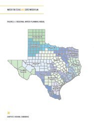
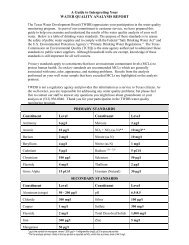
Figure 4.1.8. Monthly average inflows from 1941-1987 fot the Nueces, Mission-Aransas, Guadalupe, Lavaca 

Colorado, Trinity-San Jacinto, and Sabine-Neches estuaries. 

Figure 4.1.9. Relative fte·quency of monthly freshwater inflows to the Nueces, Mission-Aransas, Guadalupe, 

Lavaca-Colorado, Trinity-San Jacinto, and Sabine-Neches estuaries, where relative frequency is the ratio ofnumb 

er ofoccurrences offlow within the given range normalized by the maximum number ofoccurrences found in all 

ranges. 

31 

Cl 

::J 

« 

0 

W 

en 

t> 

o

Mid Corpus 

Christi Bay 

Figure 4.1.13. Saliniry measurement sires in rheNueces. Missi0'l-Aransas.Guadalupe. Lavaca-Colorado. T riniry- 

San Jacinto. and Sabine-Neches estUaries. . . ..' 

35·

Nueces 

30 

20 

10 

-e-- tbices Bay 

-..- . Mid CC Bay 

-:-e--- Redlish Bay 

--...- Nav.1t. sa 

J FMAMJJASOND J FMAMJJASOND 

Month 

Figure '4.1.17. Monthly salinity distribution for sires in the Nueces; Mission·-AransaS. Guadalupe, Uvaca 

Colorado, Trinity-San Jacinto, and Sabine-Neches estuaries, 

38

HIGH-INFLOW CONDITIONS 

LAVACA-COLORADO ESTUARY 

TRINITY-SAN JACINTO ESTUARY 

TP concentrations (mg/I) . 

LOW-INFLOW CONDITIONS 

LAVACA-COLORADO ESTUARY 

TRINITY-SAN JACINTO ESTUARY 

Figure 4.2.4. Average disrriburions of rotal phosphorous concentrations (mgll) in the Lavaca-Colorado and 

Trinity-San Jacinto estuaries during periods of high and low inflows. 

44 

RIVER

clear decrease in suspended sediment load that has continued 

through 1986. Other rivers show changes in suspended 

sediment load that do not appear to be related to human 

activities. The Lavaca, Guadalupe, and San Antonio rivers 

displayed significant changes in sediment loading in 1958, 

at the end ofa prolonged drought. The decreased sediment 

load is still evident. The Nueces River had a substantial 

decrease in suspended sediment load beginning in 1972. 

The decrease, following the largest annual inflow on record 

in 1971, was still obvious in 1986. 

Recent studies have documented reductions in the 

N ueces and Trinity delta areas that are most likely related to 

reservoir construction. Reductions in the Lavaca Delta are 

.probably not reservoir-related, and changes in the Guadalupe 

Delta seem to be parr of the normal delta constructiondestruction 

cycle. While we can relate inflow and sediment 

load quantitatively, we have only a qualitative understanding 

of the relationship between sediment loading and the 

building of deltas or maintenance of bay-borrom bathymetry. 

71

Table 5.1.1. Major categoties ofphytoplankton common in Texas estuaries, ranked by 

ordet of imponance. 

Estuary Upper bay Lower bay Reference 

Sabine-Neches greens diatoms TDWR (l981e) 

diatoms greens 

blue-greens 

Trinity- diatoms TDWR (l982b) 

San Jacinto greens 

blue-greens 

Lavaca- cryptophytes Gilmore et al. (1976), 

Colorado greens Jones et al. (1986) 

diatoms 

Guadalupe cryptophytes Matthews et aI. (1975) 

greens 

diatoms 

Mission- blue-greens diatoms Holland et al. (1975) 

Aransas greens dinoflagellates 

greens 

Nueces blue-greens diatoms Holland et al. (1975) 

diatoms dinoflagellates 

Laguna Madre diatoms diatoms TDWR (1983) 

dinoflagellates greens 

5.1 ESTUARINE PHYTOPLANKTON, PRIMARY 

PRODUCTMTY, AND FRESHWATER INFLOWS 

Introduction 

The production of biomass by phytoplankton (suspended 

micro-algae) inhabiting the estuaries is a major 

source oforganic material entering the estuarine food chain. 

This section describes current information on phytoplankton 

in Texas estuaries, the importance oftheir productivity, 

and how the phytoplankton are influenced by environmental 

factors including the quality and quantity of freshwater 

inflows. 

Plankton Groups and Biomass 

Composition. The phytoplankton comprise a diverse' 

assemblage of algal species, sizes, and shapes, with various 

capacities for photosynthetic conversion of sunlight and 

dissolved nutrients into organic matter. Marine species and 

freshwater species mix in the estuaries. The relative composition 

of these species in a bay varies seasonally, to some 

extent, and as the salinity gradient changes. For the purpose 

ofassessing the general character ofestuarine primaty production, 

phytoplankton species are often grouped by major 

taxonomic divisions. The relative importance of these 

74 

groups may indicate the ecological health and functioning of 

the system, how accessible the production is to consumers, 

and whether the system may be dominated by marine or 

freshwater species. 

Table 5.1.1 presents an overview ofthe predominant 

phytoplankton groups in each estuary, summarized ftom the 

references listed. The table illustrates only the most general 

level ofcontrast. However, differences in relative dominance 

ofphytoplankton groups amongthe estuaries may determine 

which pathways are most important in moving the 

photosynthetic carbon into higher trophic levels. Diatoms, 

for example, are generally considered a more available food 

source for zooplankton than blue-green or many green algae 

(Ryther and Officer 1981). Marine diatoms are more 

prevalent in the bays ofthe lower coast than in the other bays, 

and are generally most prevalent in the portions ofthe bays 

proximal to the barrier islands. Therefore, phytoplankton 

productivity. in these bays contribute directly to the 

zooplankton link in the food chain. Freshwater algal species 

may dominate the upper bays during times ofhigh inflow. 

Because some freshwater phytoplankton species are not the 

preferred food ofzooplankton, they may enter the estuarine 

food chain through benthic filter feeders, rather than through 

the planktonic food chain.

captured and held at 30%0 for three weeks to acclimate to 

laboratory conditions: Then the saliniry was altered in steps 

of5%0 per day so that four saliniry groups were established 

in holding tanks, 10,20,35, and 450/00. Temperature and 

photoperiod were chosen to reflect spring conditions, and 

samples were taken at the end of 30 and 60 days. The 

experimental design included replicate tanks for error analysis. 

Thomas and Boyd sampled gonadal steroids (estradiol 

and testosterone), made histological examinations of gonadal 

tissue, and used a gonadosomatic index (GSI), which 

is the ratio ofthe gonad weight to the bodyweight expressed 

. as a percent, to evaluate reproductive status. 

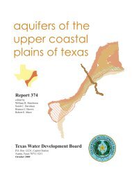
Figure 6.5.1 compares gonadosomatic indexes in successive 

30-day periods for spotted seatrout. The ratio ofthe 

gonadosomatic index for animals after 30days and the index 

for control animals (collected before the acclimation period) 

shows that initial ovarian development is sensitive to accli- 

. mation saliniry. Ovarian growth was highest for animals 

held at 350/00, followed in order by 45,20, and 100/00. The 

GSI for females held at 350/00 at the end of 30 days was 

significantly higher than the control GSI. 

In the next 30-day period, seatrout held at 100/00 did 

not survive through the end ofthe experiment. The relative 

ovarian growth for fish held at 20,35, and 450/00 was very 

similar, however, and was lower in the second 30-dayperiod 

than in the first 30days (Figure 6.5.1). Attheendof60 days, 

GSI's of both the 35 and 450/00 females were significantly 

higher than GSI's offemales from the corresponding salinities 

at the end ofthe first 30 days. 

Similar results were demonstrated by the gonadal 

steroid measurements, with 350/00 fish having the highest 

levels ofboth estradiol and testosterone. In relative terms, 

the changes in ovarian growth and gonadal steroids for the 

holding salinities were greater for the first 30-day period 

than for the second 30-day period. In addition, microscopic 

examination of ovaries showed that 350/00 females had a 

higher proportion of ooeytes developing into eggs than 

females held at the other salinities. Thus, fecundiry 0050/00 

females was higher than for the other saliniry groups due to 

greater ovarian growth and greater development ofooeytes 

into eggs. 

Thomasand Boyd concluded thatovarian growth and 

endocrine function in female spotted seatrout is significantly 

altered over the saliniry range of20 to 450/00, although 

the greatest saliniry effect appears to be in the early period of 

ovarian development. Salinities of 350/00 appeared to be 

optimal, while lower salinities (200/00 or less) suppressed 

ovarian growth and caused more reproductive interference 

than higher salinities (450/00). Theyalso looked at the effects 

ofsalinity on male spotted seatrout reproduction but con- 

6 

(J) 

Q) 

x 5 

Q) 

"0 

.!: 4 

OU 

o+" 

.- ell 

roE 

167 

3 

II: 0 (J) 

0 2 

"0 ell 

c: 

00> 

• 10 %0 

1ZI 20%0 

El 35 %0 

EJ 45%0 

o Growth in first 30 days Growth in second 30 days 

(30-day GSI/control GSI) (60-day GSI/30-day GSI) 

30-day 

Figure 6.5.1. Ratio ofthe gonadosomatic index at the end ofthe 30-day 

growth period with the gonadosomatic index from the beginning of the 

period, showing the relative amount ofgrowth ofthe ovaries compared to 

the body weight for spotted seatrour; the four bars on the left show the 

relative ovarian growth under four salinity regimes during the first 30 days 

of gonadal development; the three bars on the right show rhe relative 

ovarian growth during the next 30 days, before spawning; females held at 

100/00 did not survive the, second 30-day period (data from Thomas and 

Boyd 1989). 

cluded that it was not significantly changed over the 20 to 

450/00 salinity range. 

Atlantic croaker. Thomas and Boyd (1989) did 

similar studies with Atlantic croaker. Animals were held for 

three weeks at 300/00; then, salinities offive groups ofanimals 

were adjusted over a 10-day period to 5, 15, 25, 35, and 

450/00. Photoperiod and temperature were selected to simulate 

fall conditions. The experiments, first done in 1987, 

were repeated in 1988; samples were taken 22 to 25 days 

after the holding salinities were established. Thomas and 

Boyd noted that they were unable to capture croaker in the 

earliest stages ofovarian development for a direct comparison 

with seatrout; in 1987, the croaker ovaries were in a more 

advanced stage ofrecrudesence (ovarian development) at the 

beginning of the experiment than for the spotted seatrout 

experiments. 

In 1987, there were no significant differences among 

the fish held at different salinities for GSI (Figure 6.5.2) or 

for the gonadal steroids testosterone and estradiol. In the 

1988 experiments, however, GSI was significantly lower for 

fish held at 25 and 450/00 than for those held at 5 and 350/00 

(Figure 6.5.2). Estradiol levels and the proportion ofoocytes 

that would develop into eggs were lower for high-holding 

salinities than for low-holding salinities. 

Thomas and Boyd concluded that ovarian development 

in croaker in the last three to· four weeks prior to 

spawning is relatively insensitive to different salinities in the 

5 to 350/00 range. Holding tank salinities of450/00 may result

I' . 

Antecedent (lag) period ,in: years 

Harvest, Black drum. 

I Harvest I Red drum 

I Harvest· . Seatrout 

Harvest .Eastern oyster 

Harvest Blue crab 

Harvest .Brown, pink, and 

white shrimp 

.Harvest 

year 

Figure 6.8.3. Alignment of independent and dependent variables in (he fisheries analyses. 

,196

Table 7.6.6. (continued) Mean catch per sample for organisms caught in upper (area I). mid (area 2). and lower (area 3) San Antonio Bay and Espiritu Santo Bay (area 4) by TPWD Coastal Fisheries Monitoring Program. 

Area Scientific Name Common Name 

M 

Gillnet 

SE n M 

Mean (M), standard error (SE), and sample size (n) Percent ofsamples 

Trawl 

SE n M 

Bag seine 

SE n 

Oyster dredge 

M SE n· 

GilInet 

Trawl Bag 

seine 

4 . Carcharhinus kucas Bull shark 0.82 0.11 313 31.3 

2 Carcharhinus /imbatus . Blacktip shark 0.00 0.06 262 0.38 

3 Carcharhinus /imbatus Blacktip shark 0.00 0.06 298 0.34 

4 Carcharhinus /imbatus Blacktip shark 0.02 0.01 313 1.60 

3 Carcharhinus p/umbeus Sandbar shark 0.03 0.02 298 0.67 

4 Carcharhinus p/umbeus Sandbar shark 0.00 0.06 313 0.32 

1 

2 

3 

4 

4 

Chaetodipterus faber 




Chasmodes bosfjuianus 

Atlantic spadefish 




Striped blenny 

0.01 

O.ol 

0;00 

0.08 

0.12 69· 

0.12 262 

0.06 298 

0.02 313 

0.01 

0.01 

0.00 

0.01 

0.00 

0.G5 

825 

348 

348 

0.01 

0.00 

0.00 

0.04 

544 

544 

1.45 

Q.38 

0.34 

5.43 

0.36 

0.86 

0.29 

0.37 

0.18 

3 Chelonia mydAs Green sea turtle 0.00 0.06 298 0.34 

N 

'" 

4 

4 

2 

Chilomycterus schoepfi 

Chione canu//ata 

Chloroscombrus chrysurus 

Srriped burrfish 

Cross-barred venus 

Atlantic bumper 

0.00 

0.01 

0.05 348 

0.01 402 

0.01 0.10 103 

0.29 

0.50 

0.97 

00 3 

4 

1 

2 

3 

4 

3 

2 

3 

4 

2 

3 

4 

1 

2 

3 

4 

1 

2 

3 

4 

1 

2 

3 

4 

2 

4 

1 



CitharichthYllpilopterus 

CitharichthYl spilopterus 

CitharichthYl Ipilopterul 

CitharichthYl spilopterus 

Class Osteichthyes 

.Class Polychaeta 

Class Polychaeta 

,Class Polychaeta 

.C/ibanarius vittatul 

C/ibanarius vittatus 

.C/ibanarius vitlatus 

Table 7.6.6. (continued) Mean catch per sample for organisms caught in upper (area 1), mid (area 2), and lower (area 3) San Antonio Bay and Espiritu Santo Bay (area 4) by TPWD Coastal Fisheries Monitoring Program. 

Area Scientific Name Common Name 

M 

Gillnet 

SE n M 

Mean (M), standard error (SE), and sample size (n) Percent ofsamples 

Trawl 

SE n M 

Bag seine 

SE n M 

Oyster dredge 

SE n 

Gillnet 

Trawl Bag 

seine 

3 Sciamops ocellatus Red drum 7.51 0.54 298 . 0.01 0.00 825 0.53 0.09 '456 83.6 0.61 16.4 

4 Sciamops ocellatus Red drum 10.7 0.62 313 0.00 O.os 348 0.67 0.12 544 91.4 0.29 19.5 

4 Scomberomorus cavalla King mackerel 0.00 0.04 544 0.18 

2 Scomberomorus maculatus Spanish mackerel 0.05 0.74 262 '0.38 

4 Scomberomorus maculatus Spanish mackerel 0.01 0.01 313 0.00 0.04 544 0.96 0.18 

2 Selme utapinnis Atlantic moonfish 0.00 0.05 402 0.25 

3 Seune. utapinnis Atlantic moonfish 0.00 0.03 825 0.12 

4 Seune utapinnis Atlantic moonfish 0.08 0.03 348 3.45 

2 Selme vomer Lookdown 0.00 0.05 402 0.25 

3 

4 

Seune vomer 

Seune vomer 

Lookdown 

Lookdown 0.02 0.01 313 

0.00 

0.G3 

0.03 825 

0.01 348 0.64 

0.12 

2.30 

N 

C\ 

'-l 

4 

4 

2 

3 

4 

4 

4 

1 

2 

3 

4 

2 

3 

4 

3 

4 

1 

2 

3 

4 

Sicyonia brevirostris 

Sicyonia dorsalis 

Sphoeroitks parvus 



Sphomitks spmgleri 

Sphyrna lewini 

Sphyrna tiburo 




Squilla empusa 



Stelljftr lanceolatus 

Stelljftr lanceolatus 

Stomolophus mekagris 

.Stomolophus mekagris 

Stomolophus meuagris 

Stomolophus meleagris 

Rock shrimp 

Lesser rock shrimp 

Least puffer 

Least puffer 

Least puffer 

Bandtail puffer 

Scalloped hammerhead 

Bonnethead 

Bonnethead 

Bonnethead 

Bonnethead 

Mantis shrimp 

Mantis shrimp 

Mantis shrimp 

Star drum 

Star drum 

Cabbagehead 

Cabbagehead 

. Cabbagehead 

Cabbagehead 

0.01 

0.81 

0.12 

0.48 

0.00 

O.oI 

0.12 69 

0.81 262 

0.05 298 

0.13 313 

0.06 298 

O.oI 313 

0.00 

0.06 

0.12 

0.05 

0.00 

0.00 

0.00 

0.01 

0.04 

0.03 

4.79 

2.03 

0.25 

O.os 348 

0.02.402 

0.G3 825 

0.02 348 

0.05 348 

0.05 348 

0.00 402 

O.oI 825 

0.01 348 

0.02 825 

2.29 402 

0.45 825 

0.09 348 

0.00 

0.09 

0.35 

0.G9 

0.00 

0.31 

0.22 

0.18 

0.00 

0.04 

0.04 

0.15 

0.05 

0.04 

0.28 

1.91 

0.15 

0.09 

544 

78 

456 

544 

544 

65 

78 

456 

544 

0.03 

0.0.1 

0.53 

0.10 

349 

103 

1.45 

0.76 

4.03 

14.4 

0.34 

0.64 

0.29 

3.73 

5.58 

4.31 

0.29 

0.29 

0.50 

0.85 

2.87 

0.48 

8.71 

12 

6.32 

0.18 

7.69 

7.89 

2.94 

0.18 

3.08 

1.28 

0.88 

0.18 

0.29 

0.97 

2 Strongylura marina Atlantic needldish 0.01 0.01 262 0.G3 0.02 78 0.76 2.56 

3 Strongylura marina Atlantic needlefish 0.00 0.06 298 0.06 0.02 456 0.34 3.73 

4 Strongylura marina Atlantic needlefish 0.00 0.06 313 0.08 0.04 544 0.32 2.21 

2 Suborder Reptanria Suborder reptantia 0.00 0.05 402 . '0.25 

4 _Suborder Reptantia Suborder reptantia 0.00 0.04 544 . 0.18 

2 Symphurus plagiusa Blackcheek ronguefish 0.01 0.01 402 1.00 

3 Symphurus plagiusa Blackcheek tonguefish 0.01 0.00 825' 0.03 O.oI 456 1.21 (.54 

4 Symphurus plagiusa . Blackcheek tonguefish 0.01-. O.oI 348 0.G3 0.01 544 0.86 2.39 

1 Syngnathus florid/It Dusky pipefish 0.02 '0.12 65 1.54 

3 Syngnathus fIoridae Dusky pipefish 0.00 . 0.05 456 0.22 

.4 Syngnathus fIoridae Dusky pipefish 0.00 0.04 544 0.18 

2 Syngnathus Iouisianae Chain pipefish . 0.00. 0.10 402 0.25 

Oyster 

dredge 

.;4

Table 7.6.6. (concluded) Mean catch per sample for organisms caught in upper (area I), mid (area 2), and lower 5area 3) San Antonio Bay and Espiritu Santo Bay (area 4) by TPWD Coastal Fisheries Monitoring Program. 

. .. 

Area Scientific Name 

Common Name· 

Mean (M), standard error (SE), and saO!ple size en) Percent ofsamples 

Gillnet Trawl Bag seine Oyster dredge Gill- Trawl Bag Oyster 

net seine dredge 

M SE n M SE n M SE n M SE n 

3 Syngnathus u,';isianae Chain pipefish 0.00 0,03 825 0.01 0.19 456 0.12 0.22 

4 

2 

Syngnathus u,uisianae 

Syngnathus scovelli 

Chain pipefish 

Gulf pipefish 0,02 0.01 402 

0.01 

0.06 

0.01 

0.03 

544 

78 O.oI 0.11 349 1.00 

0.92 

5.13 0.29 

3 Syngnathus scovelli Gulfpipefish 0.01 0.00 825 0.06 0.02 456 0.61 4.82 

4 Syngnathus scovelli Gulf pipefish 0.09 0.02 544 5.51 

3 SynoJus foetms Inshore Iizardfish 0.01 0.00 825 0.02 0.01 456 1.09 1.32 

4· SynoJus foetens Inshore lizardfish 0.01 0.01 348 0.01 0.00 544 1.15 0.92 

2 Thais haemastoma Florida rock shell 0.00 0.05 402 0.25 

4 Thais haemastoma Florida rock shell 0.01 0.01 348 0.01 0.10 103 1.15 0.97 

3 Touuma caro/inmse Arrow shrimp 0.00 0.05 456 0.22 

2 Trachinotus caro/inus Florida pompano 0.02 0.02 262 0.76 

3 

4 

Trachinotus ca"ro/inus 

Trachinotus caro/inus 

Florida pompano 

FlorIda pompano 

0,03 

0.08 

0.01 298 

0,02 313 0,02 0.01 544 

2.01 

5.43 1.10 

4 Trachinotus fakatus Permit 0.02 0.01 313 0.96 

to.> 

0\ 

00 

3 

3 

Trachinotus goodei 

Trachypmaeus simi/is 

Palometa 

Yellow rough-necked 

shrimp 

0.00 0.06 298 

0.00 0.03 825 

0.34 

0.12 

3 Trachypmaeus sp. Trachypeneid 0.00 0.03 825 0.12 

'2 

3 

4 

I 

2 

.3 

4 

I 

Trichiurus kpturus 

Trichiurus kpturus 

Trichiurus /epturus 

Trinectes maculatus 


Trinectn maculatus 


Tursiopi truncatus 

Atlantic cutlassfisn 

Atlanticcutlassfish 

Atlantic cutlassfish 

Hogchoker 

Hogchoker 

Hogchoker 

Hogchoker 

Atlantic bottlenose 

dolphin 

0.04 

0.03 . 

0.06 

0.04 

O.oI 

, , 

0.02 69 

0.01 262 

0.01 298 

0.01 313 

0.12 69 

0.00 

0.01 

0.08 

0.11 

0.11 

0.06 

0.03. 

0.05 402 

0.00 825 

0.02 348 

0.07 66 

0,02 402 

O.oI 825 

0.01 348 

0.06 

O.oI 

0.01 

0.04 

0.01 

0.01 

78 

456 

544 

4.35 

2.29 

6.04 

2.88 

1.45 

0.25 

0.97 

4.60 

4.55 

6.97 

4.36 

2.30 

3.85 

0.66 

1.10 

3 

4 

Urophycis floriJana 

UrophycisfloriJana 

Southern hake 

Southern hake 

0.01 

0.03 

0.00 825 

0.01 348 

1.21 

2.01

276

( 1 fps: ) 

Figure 8.4.3. Simulated velocity vectors for the Three-Bay Model at OOOOhr on June 28, 1984; arrow 

indicates a velocity of 1 ftls. 

296

( 1 fps: ) 4329HOURS 

Figure 8.4.6. Simulated velocity vectors for the Three-Bay Model at 0900 hr on June 28,1984; arrow 

indicates a velocity of 1ftls. . '. ., 

299

( 1 fps: ) 4335HOURS 

Figure 8.4,8, Simulatcdvelocity vect()ts for the Three-Bay Model at 1500hr on June 28. 1984; arrow 

indicates a velocity of 1 ft/s. 

301

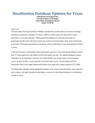
Three Bay System: 1984 simulation 

Figure 8.4.16. IsoilaJinesof,the sim$tedsalinitf from the Three-Bay Model for March 1984. 

309 

MONTH: 3

Thl'ee Boy ,Systerr,: 1984 simulation tv10f'1TH: 4 

. Figure 8.4.17. lsohalines of me simiilated salinity from the Three-Bay Model for April 1984. 

310

Three Boy System: 1984 simulation 

Figure 8.4.20. Isohalines ofthe simulate4 salinity from the Three-Bay Model for.July 1?84. 

313 

MONTH: 7 

,I

._-.,...----------------_.__._------ 

Three Bay SysterT1: 1984 sirnulation MONTH: 8 

Figure 8.4.21. lsohalines of the simulated salinity froll! the Three-Bay Model for Augusr 1984. 

314

.' 

Three ,Boy System: 1984 simulation MONTH:' 10 

Figurc 8.4.23. lsohalincs ofthc simulatcd salinity from thc Thrc';-Bay Model for October 1984. 

316

Three Boy System: 1984 simulation 

Figure 8.4.24. Isohalines ofthe simulated salinity.from the Three-Bay Model for November 1984. 

'317 

MONTH: 1 1

in lower San Antonio Bay. The salinity limits in the upper 

bay and in Espiritu Santo Bay did not control inflow 

amounts. 

Inflow requirements ranged from 0.9 to 1.5 million 

acre-fr/yr, depending on the species and weightings among 

the species. This is halfto two-thirds ofthe inflow requirements 

that were determined in previous srudies that were 

based on productivity maintenance goals. The miriimum 

inflow requirement (0.9 million acre-fr/yr) from this analysis 

is about 50% greater thanwas calculated by anoth.er study 

that was based only on viability limits ofestuarine organ 

Isms. 

323 

Circulation andsalinity modeL This section has also 

presented results ofa simulation ofcirculation and salinity 

conditions in the Guadalupe Estuary from the TXBLEND 

Model. The salinity values calculated by the model are 

reasonable and the general patterns ofsalinity'distribution 

are consistent with measurements taken there. In general, 

the results from the TXBLEND Model" using optimal inflows 

show thatsalinities in the zones used for the regressions 

do not substantially exceed the salinity bounds that were set 

for the TXEMP Model analysis.

this model to these dynamic constituents, however, data is 

needed on the rates of biological and chemical processes 

which affeer these materials. 

There may be a role for the optimization approach 

developed here to address future water quality concerns. 

There are trade-offs to the estuary in a future scenario of 

higher rates of nutrient loading which may come with 

increased urbanization'ofestuarine shores. Increased nutrient 

loading may bring positive increases in produerivity to 

some estuaries. However, increased nutrient loading also 

may increase risks of the development of anoxic areas, red 

tide blooms, or other problems. How these risks weigh 

against the possible increased produerivitydepends on many 

faerors, including rates ofwater exchange, seasonality, and 

faerors which limit the biological community. The framework 

ofthe TXEMP Model is uniquelysuited to incorporate 

in a quantitative way our knowledge ofthe interaerions of 

these various faerors. Water quality standards and productivity 

measures could also be included as targets or controlling 

parameters. Relationships between loading rates and 

prediered dissolved oxygen concentrations or other parameters 

could be used as constraints. It is possible to envision 

theapplicationofthis model towaterqualityconcerns in this 

way. However, to make it work, more detailed knowledge 

, is required ofthe best way to express relationships between 

nutrient loading, pollutantconcentrations, and the behavior 

ofthe estuarine ecosystem. 

Conclusion 

The models and methods needed to use the analytical 

procedure to determine freshwater inflow requirements 

have been developed. Most of the information about the 

hydrology of inflowing waters and fishery equations is also 

available. The models ofcirculation and conservative transport 

for several estuaries need to be calibrated, and the 

nutrient budgets using cumulative flows from these models 

must still be prepared. Analyses ofsediment requirements 

for the bay systems other than the Guadalupe Estuary will 

have to be done on a case-by-case basis, probably aimed at 

determining sediment requirements for maintaining delta 

wetlands. 

Several enhancements to the method were discussed 

including improved primary produerivity relationships and 

the addition of benthic produerivity and water quality 

components. Because the analytical procedure is somewhat 

modular, incremental improvements to the analytical procedure 

as well as new features can be added easily at any time. 

Some ofthe techniques and analyses can be applied to other 

important problems such as the responses ofecosystems to 

unusual occurrences or deleterious changes from major 

pollutantspills, eutrophication,ortoxic algae blooms. There 

may be concern over the length oftime required for a bay to 

flush out a pollutant, or the question might be whether 

Currents will sweep a red tide bloom into a bay. The 

morphometry of passes, the orientation of ship channels, 

and the volume of freshwater inflows all influence the 

exchange between major secondary and tertiary bays and the 

circulation of fresh and salty water within the bays. The 

models presented here provide a way ofcombining information 

on manyaspects ofestuaryhydrodynamics, movements 

of materials, and ecological processes. 

9.3 POUCY DECISIONS THAT MUST BE MADE 

TO APPLY THE METHODOLOGY 

Introduction 

In response to statute direerives for studies on the 

effeers of freshwater inflows, state scientists and engineers 

have developed a comprehensive database and methodology 

for estimating the freshwater inflow needs ofTexas bays and 

estuaries. Since freshwater inflows affeer' our estuarine 

(tidal) systems at all basic levels of interaction-physical, 

chemical, and biological effeers--the new method was designed 

to include at least the minimum needs for each 

functional level. It also incorporates a technique for optimizing 

the freshwater inflow needs across all levels ofinteraerion 

to maintain the ecological integrity ofthese valuable 

coastal environments. 

The TXEMPModeL The TXEMP Model was cooperatively 

developed and tested with the Center for Research 

in Water Resources at The University ofTexas at Austin. It 

allows use ofa multiobjeerive approach to solving the inflow 

problem and incorporates the statistical uncertainty ofcorrelated 

relationships between freshwater inflows and resulting 

bay salinities and fisheries harvests. This is a real 

advancement in this type of solution technique. Model 

results are displayed as "performance curves" like the illustrative 

examples shown in Figure 9.3.1. From these performance 

curves, decision-makers can select the point that best 

balances the needs of man and the environment for the 

benefit ofall Texans. As a final check, the freshwater inflow 

needs calculated by the TXEMP Model are incorporated 

, into the TXBLEND hydrodynamic model to evaluate the 

overall effeers on bay circulation and salinity patterns. 

342 

Policy decisions and 11Ulnagement objectives. While 

the logic and equations ofthe optimization model are built 

on scientific and engineering analyses, application of the 

model requires the mathematical expression ofall operative 

constraints, limits, and state resource management objectives. 

Decisions about these objeerives are in the realm of 

public policy, more than science and engineering. They are

346

Espey, Huston & Associates, Inc. 1986. Water availability study for the Guadalupe and San Antonio river basins. Repon 

to San Antonio River Authority, Guadalupe River Authority, and City of San Antonio, by Espey, Huston &. 

Associates, Austin, TIC. DocUment No. 85580. 

Eczold, D.J., and J.Y. Christmas. 1977. A comprehensive summary ofthe shrimp fishery ofthe GulfofMexico, United 

States: a regional management plan. GulfCoast Res. Lab. Tech. Rep. Ser. No.2. 20 pp. 

Etzold, D.J., and J.Y. Christmas. 1979. A Mississippi marine finfish management plan. Mississippi-Alabama Sea Grant 

Consonium. MASGP-78-046. 

, 

Ewald, J.J. J 965. The laboratoty rearing ofpink shrimp, Penaros duorarum Burkenroad. Bull. Mar. Sci. 15:436-449. 

Fable, W.A., Jr., T.D. Williams, and e.R.Arnold. 1978. Description ofreared eggs and young larvae ofthe sponed seatrout, 

Cynoscion nebulosus. U.S. Natl. Mar. Fish. Servo Fish. Bull. 76:65-71. 

Failing, M.S. 1969. Comparison ofTrinity River terraces and gradients with other Texas Gulfcoast rivers. Pages 85-92 

in R.R. Lankford and J.J. W. Rogers, eds. Holocene geology ofthe Galveston Bay area. HOlLsron Geological Society, 

Delta Study Group. .. 

Farley, O.H. 1963-1969. Texas landings: annual summary, 1962-1968. Bureau of Commercial Fisheries, U.S. 

Depanmentofthe Interior, and Texas Parks and Wildlife Depanment. Current Fisheries Statistics Nos. 3309, 3627 

revised, 3901,4156,4529,4675, and 4962. 

Farley, a.H. 1970-1978. Texas landings: annual summary, 1969-1976. National Marine Fisheries Service, U.S. 

DepartmemofCommerce, and Texas Parks and Wildlife Department. Current Fisheries Statistics Nos. 5232, 5616, 

5923,6124,6423,6723,6923, and 7223. . 

Farrell, R. 1980. Methods for classifYing changes in environmental conditions. Tech. Rep. VRF-EPA7.4-FR80-1. Vector 

Research, Inc. Ann Arbor, MI. 

* Fensenmaier, D.R., T. Ozuna, Jr., S. Urn, L.L. Jones, W.S. Roehl, RQ. Guajardo, and A.S. Mills. 1987. Regional and 

statewide economic impacts ofspon fishing, other recreational activities, and commercial fishing associated with 

·major bays and estuaries of the Texas Gulf coast. Repon to Texas Water Development Board, by Depanment of· 

Recreation and Parks and Department ofAgricultural Economics, Texas A&M University, College Station, TX. 

Execl!tive summary + 6 regional repons. . 

Finucane, J.H., L.A. Collins, and L.E. Barger. 1978. Spawning ofthe striped mullet (Mugil aphalus) in the nonhwestern 

Gulf of Mexico. Nonheast GulfSci. 2(2):148-150. 

Fisher, T.R., L.W. Harding, Jr., D.W. Stanley, and L.G. Ward. 1988. Phytoplankton, nutrients, and turbidity in the 

Chesapeake, Delaware, and Hudson estuaries. Estuarine Coastal Shelf Sci. 27:61-93. 

Fisher, W.L. 1969. Facies characterization ofGulfcoast basin delta systems, with some Holocene analogues. GulfCoast 

Associarion of Geological Societies Transactions 19:239-261. 

Fisher, W.L., ].H. McGowen, L.F. Brown, Jr., and e.G. Groat. 1972. Environmental geologic atlas ofthe Texas coastal 

zone-Galveston-Houston area. Bureau ofEconomic Geology, University ofTexas at Austin, Austin, TX. 91 pp. 

+ 9 plates. 

Fleeger, J.W., W.B. Sikora, and J.P. Sikora. 1983. Spatial and long-term temporal variation ofmeiobenthic-hyperbenthic 

copepods in Lake Ponchanrain, Louisiana. Estuarine Coastal Mar. Sci. 16:441-453. 

Flint, R.W. 1984. Phytoplankton production in the Corpus Christi Bay Estuary. Contrib. Mar. Sci. 27:65-83. 

356

Hildebrand, RH., and G. Gunter. 1953.. Correlation of rainfall with Texas catch of white shrimp, Penaeus seti/er:us 

(Linnaeus). Trans. Am. Fish. Soc. 82:151-155. 

Hines, S.D., H.A. Debaugh, Jr., and L.E. Hickman, Jr. 1987. Population dynamics and habitat partitioning by size and 

sex and molt stage ofblue crabs, Callinectes sapidus, in a sub-estuary ofcentral Chesapeake Bay. Mar. Ecol. Prog. Ser. 

36:55-64. . 

Hirsch, R.M., }.M. Slack, and R.A. Smith. 1982. Techniques of trend analysis for monthly water quality data. Water 

Resour. Res. 18:107-121. 

Hjort, J. 19 j 4. Fluctuations in the great fisheries ofnorthern Europe viewed in the light ofbiologic;U research. Rapp. P.- 

V. Reun. Cons. Int. Explor. Mer. 20: 1-228. . 

Hoese, H.D. 1960. Biotic changes in a bay associated with the end ofa drought. Limnol. Oceanogr. 5(3}:326-336. 

Hofsrerrer, R.P. 1959. The Texas oyster fishery. Texas Parks and Wildlife Department, Austin, TX. Bulletin No. 40 

(revised 1964). 36 pp. 

.Hofsterrer, R.P. 1977. Trends in population levels ofthe American oyster, Crassostrea virginica (Gmelin), on public reefs 

in Galveston Bay, Texas. Coastal Fisheries Branch, Texas Parks and Wildlife Department, Austin, TX. Pub. No. 

24. 90 pp. 

Hofstetter, R.P. 1983. Oyster population trends in Galveston Bay, 1973-1978. Coastal Fisheries Branch, Texas Parks and 

Wildlife Department, Austin, TX. Management Data Series No. 51. 

Holcomb, H.W.,Jr. 1970. An ecological study ofthe gulfmenhaden (Brevoortiapatronw) in a low-salinity estuary in Texas. 

M.S. Thesis. Texas A&M University, College Station, TX. 47 pp. . 

Hobon, G.F. 1974. Metabolic cold adaptation ofpolar fishes: fact or artifact? Physiol. Zoo!' 47: 137-152. 

Holland, J.S., D.V. Aldrich, and K. Strawn. 1971. Effects oftemperature and salinity on growth, food conversion, survival 

and temperature resistence ofjuvenile blue crabs, Callinectes sapidus Rathbun. Texas A&M Univ. Sea Gtant Pub!. 

TAMU-SG-71-222. 166 Pl" 

'" Holland, J.S., N.J. Maciolek, R.D. Kalke, L. Mullins, and C.H. Oppenheimer. 1973a. A benthos and plankton study of 

the Corpus Christi, Copano and Aransas bay systems I. Report on rhe methods used and data collecred during the 

period September, 1972 - June, 1973. Report ro Texas Water Development Board, by Marine Science Insticure, 

. University ofTexas at Austin, Port Aransas, TX. 220 Pl" 

*' Holland, J.S., N.J. Maciolek, R.D. Kalke, L. Mullins, and C.H. Oppenheimer. 1974. A benthos and plankton study of 

the Corpus Christi, Copano and.A..ransas bay systems II. Report on data collected during the period]uly, 1973 - April, 

1974. Report to Texas Water Development Board, by Marine Science Institute, University ofTexas at Austin, Port 

Aransas, TX. 121 Pl" . 

'" Holland, J.S., N.]. Maciolek, R.D. Kalke, L. Mullins, andC.H. Oppenheimer. 1975. A benthos and plankron study of 

the Corpus Christi, Copano andAransas bay systems III. Report on data collected during the period July, 1974 - May, 

1975 and summary of the ·three-year project. Report to Texas Water Development Board, by Marine Science 

Institute, University ofTexas at Ausrin, Pon Aransas, TX. 174 Pl" 

Holland, J.S., N.J. Maciolek, and C.H. Oppenheimer. 1973b. Galveston Bay benthic coinmunitystructure as an indicator 

ofwater quality. Contrib. Mar. Sci. 17:169-188. 

Holley, E.R. 1991. Sediment transport in the lower Guadalupe and San Antonio rivers. Center for Research in Water 

Resources, University ofTexas at Austin, Austin, TX. Technical Memorandum 91-1. 

361

Menzel, R W., N.C. Hulings, and RR Hathaway. 1966. Oyster abundance in Apalachicola Bay, Florida, in relation to 

biotic associations influenced by salinity and other factors. GulfRes. Rep. 2:73-96. 

Mercer, L.P. 1984. A biological and fisheries profile of red drum, Sciaenops oce/latus. Repon to V.S. Department of 

Commerce, National Marine Fisheries Service, by North Carolina DepartmentofNatural Resources, Morehead City, 

NC. 90 pp. 

Miglarese, J.V., and M.H. Shealy, Jr. '1982. Seasonal abundance ofAtlantic croaker (Micropogonias undulatus) in relation 

to bottom salinity and temperature in South Carolina estuaries. Estuaries 5(3):216-223. 

Millikin, M.R., and A.B. Williams. 1984. Synopsis ofbiological data on the blue crab, Callinectes sapidus Rathbun. NOAA 

. Tech. Rep. NMFS 1. 39 pp. 

Milliman, J.D., and R.H. Meade. 1983. Worldwide delivery ofriver sediments to the oceans. Journal ofGeology 91 (1): 1 

21. 

Minello, T.]., and R.J. Zimmerman. 1983. Fish predation on juvenile brown shrimp, Penaeus aztecus Ives: the effect of 

simulated Spanina structure on predation rates. J. Exp. Mar. Bio!. Eco!. 72:211-231. 

Minello, TJ., and R.]. Zimmerman. 1985. Differential selection for vegetative structure between juvenile brown shrimp 

(perzaeus aztecus) and white shrimp (P. setiftrus), and implications in predator-prey relationships. Estuarine Coastal 

ShelfSci. 20:707-716. 

Minello, TJ., R.]. Zimmerman, and P. Barrick. 1990. Experimental studies on selection for vegetative structure by penaeid 

shrimp. National Marine Fisheries Service, U.S. Department of Commerce. Technical Memorandum NMFS 

SEFC-237. 30 pp. 

Minello, TJ., R]. Zimmerman, and TE. Czapla. 1989. Habitat-related differences in diets ofsmall fishes in Lavaca Bay, 

Texas, 1985-1986. National Marine Fisheries Service, U.S. Department ofCommerce. Technical Memorandum 

NMFS-SEFC-236. 16 pp. . 

. Minello, T]., RJ. Zimmerman, and E.X. Maninez. 1987. Fish predation on juvenile brown shrimp, Penaeus aztecus: 

Effects of turbidity and substratum on predation rates. U.S. Natl. Mar. Fish. Servo Fish. Bull. 85:59-70. 

Monaco, M.E., T.E. Czapla, D.M. Nelson, and M.W. Pattillo. 1989. NOAA's estuarine living marine resources project: 

distribution and abundance of fishes and invertebrates in Texas estuaries. National Oceanic and Atmospheric 

Administration, U.S. Depanmenr of Commerce. 107 pp. 

.. Montagna, P.A., and RD. Kalke. 1989a. A synoptic comparison ofbenthic communities and processes in the Guadalupe 

and Lavaca-T res Palacios estuaries, Texas. Repon to Texas Water Development Board, .by Marine Science Institute, 

University ofTexas at Austin, Pon Aransas, TX. 35 pp. . 

.. Montagna, P.A., and R.D. Kalke. 1989b. The effect offreshwater inflow on meiofaunal and macrofauna] populations in 

San Antonio, Nueces, and Corpus Christi bays, Texas. Repon to Texas Water Development Board, by Marine 

Science Institute, University ofTexas at Austin, Pon Aransas, TX. 34 pp. 

Montagna, P.A., and R.D. Kalke. 1992. The effect offreshwater inflow on meiofaunal and macrofaunal populations in the 

Guadalupe and Nueces estuaries, Texas. Estuaries 15:307-326. 

.. Montagna, P.A., and W.B. Yoon. 1989. The effect offreshwater inflow on meiofaunal consumption ofsediment bacteria 

and microphytobenthos in San Antonio Bay, Texas. Repon toTexas Water Development Board, by Marine Science 

Institute, University ofTexas at Austin, Pon Aransas, TX. 27 pp. 

369

Parker,].C 1970. Distribution ofjuvenile brown shrimp (Pmaeusaztecus Ives) in Galveston Bay, Texas, as related to cenain 

hydrographic features and salinity. Contrib. Mar. Sci. 15:1-12. 

Parker, J.C 1971. The biology ofspot, Leiostomus xanthurus Lacepede, and the Atlantic croaker, Micropogon uiuJulatus 

(Linnaeus), in two GulfofMexico nursety areas. Texas A&M University. Sea Grant Publ. TAMU-SG-71-210. 

* Parker, P.L., KH. Dunton, R.S. Scalan, and R.K Anderson. 1989. Final integrated repon, stable isotope component. 

Repon to Texas Water Development Board, by Marine Science Institute, University ofTexas atAustin, PonAransas, 

TX. 20 pp. + 26 figs. 

Parker, R.H. 1955. Changes in the invenebrate fauna, apparently anributable to salinity changes, in the bays ofCentral 

Texas. Journal ofPaleont. 29:193-211. 

Parker, R.H. 1959. Macroinvenebrate assemblages ofCentral Texas coastal bays and Laguna Madre. Am. Assoc. Petrol. 

Geol. Bull. 43:2100-2166. 

Pearson, J.C 1929. Natural history and conserVation ofredfish and other commercial sciaenids on the Texas coast. Bull. 

U.S. Bur. Fish. 4:129-214. 

Pearson, J.C 1948. FJuctuations in the abundance ofthe blue crab in Chesapeake Bay. U.S. Fish WildL Servo Res. Rep. 

No. 14. 26 pp. 

Perez-Farfame, I. 1969. Western Atlantic shrimps ofthe genus Penaeus. U.S. Fish Wildl. Servo Fish. Bull. 67(3):461-591. 

Perez-Farfante, I. 1988. Illustrated key (0 penaeid shrimps ofcommerce in the Americas. NOAA Tech. Rep. NMFS 64. 

32 pp. 

Perret, W.S., W.R. Latapie, J.F. Pollard, N.R. Mock, G.B. Adkins,'W.]. Gaidry, and C]. White. 1971. Fishes and 

invenebrates collected in trawl and seine samples in Louisiana estuaries. Section I. Pages 39-105 in Cooperative Gulf 

ofMexico estuarine inventory and study. Phase IV. Biology. Louisiana Wildlife and Fisheries Commission, Baron 

Rouge, LA. 175 pp. 

Perret, W.S., J.E.Weaver, R.O. Williams, P.L. Johansen, T.D. McIlwain, R.C Raulerson, and W.M. Tatum. 1980. 

Fishery profiles of red drum and sponed seatrout. GulfStates Mar. Fish. Comm. Rep. 6. 60 pp. 

.Peters, KM., and R.H. McMichael, Jr. 1987. Early life history ofthe red drum, Sciaenops oce/latus (Pisces: Sciaenidae), 

in Tampa Bay, Florida. Estuaries lO(2}:92-107. 

Peterson, G.W. 1984. Distribution, relative abundance, and habitat preference ofjuvenile sponed seatrout and red drum 

in Caminada Bay estuary, Louisiana. Coastal Ecology and Fisheries Institute, Louisiana State Universiry, Baton 

Rouge, LA. 33 pp. (Manuscript) 

Peus, G., and I. Foster. 1985. Rivers and landscape. Edward Arnold, Baltimore, MD. 274 pp. 

Phillips, R.C i 960. Observations on rhe ecology and distribution ofthe Florida seagrasses. Fla. Board Conserv. Mar. Lab. 

Prof. Pap. Ser. 2:1-72. 

Pierce, M.E., andJ.T. Conover. 1954. Astudy ofthe growth ofoysters under different ecological conditions in.Grear Pond. 

BioI. Bull. (Woods Hole) 107:318. (Abstract) 

Polgar, T.T., 1.K Summers, R.A. Cummins, K.A. Rose, and D.G. Heimbuch. 1985. Investigation ofrelationships among 

pollutant loa;dings and fish stock levels in northeastern estuaries. Estuaries.8(2A):125-135. 

372

Schwam, F.J. 1981. Effects offreshwater runoffon fishes occupying the freshwater and estuarine coastal watersheds of 

North Carolina. Pages 282-294 in RD. Cross and D.LWilliams, eds. Proceedings ofthe National Symposium on 

Freshwater Inflow to Estuaries. Vol. I. U.S. Fish Wildl. Servo BioI. Servo Program FWS/OBS-81-04. 

Schwartz, F.J., W.T. Hogarth, and M.P. Weinstein. 1982. Marine and freshwater fishes of Cape Fear Estuary, North 

Carolina, and their distribution in relation to environmental factors. Brimleyana 7: 17-37. 

Seagle, J.H. 1969. Food habits of spotted seatrout (Cynoscion nebulosus Cuvier) frequenting turtle grass (Thalassia 

testudinum Konig) beds in Redfish Bay, Texas. TAIUS 1:58-63. 

Searcy, J.K., and CH. Hardison. 1960. Double-mass curves. U.S. Geological Survey Water Supply Paper 1541 :31-66. 

Seitzinger, S.P. 1988. Denitrification in freshwater and coastal marine ecosystems: Ecological and geochemical 

significance. Limnol. Oceanogr. 33(4):702-724. 

Sen, P.K. 1968. On a class of aligned rank order tests in two-way layouts. Ann. Math. Statist. 39: 1115-1124. 

Seneca, E.D. 1974. Germination and seedling response ofAdantic and Gulfcoast populations ofSpartina aitemij1om. Am. 

. . J. Bot. 61 (9):987.. 

Sharp, .I.H., ).R. Pennock, T.M. Church, J.M. Tramontano, and LA. Cifuentes. 1984. The estuarine interaction of 

nutrients, organics, and metals: a case study in the Delaware Estuary. Pages 241 - 260 in V.R. Ktnnedy, ed. The 

estuary as a filter. Academic Press, New York, NY. 511 pp. 

Shaw, R.F., J.H. Cowan, Jr., and T.L. Tillman. 1985. Distribution and density of Brevooftia pammus (gulf menhaden) 

eggs and larvae in the continental shelfwaters ofwestern Louisiana. Bull. Mar. Sci. 36(1):96-103. 

Shaw, S.P., and CG. Fredine. 1956. Wetlands ofthe United States; their extent and their value to waterfc)wl and other 

wildlife. U.S. Fish Wildl. Servo Circ. 39. 67 pp. 

Shea, G.B., G.B. Mackiernan, L.C.Athanas, and D.F. Bleil. 1980. Chesapeake Bay low-flow study: biora assessment. Phase 

I final'report to U.S. Army Corps ofEngineers, by Western Ecosysrems Technology, Laurel, MD. Vol. I and II, 326 

pp.; Vol. III, 202 pp. 

Shenker, J.M., and).M. Dean. 1979. The utilization ofan intertidal salt marsh by larval and juvenile fishes: abundance, 

diversiry, and temporal variation. Estuaries 2: 154-163. 

Shepard, F.P. 1953. Sedimentation rates in Texas esmaries and lagoons. Am. Asoc. Pet. Geo!. Bull. 37: 1919-·193 Lt. 

Shepard, F.P., and D.G. Moore. 1960. Bays ofthe central Texas coast. Pages 117-152 in F.P. Shepard, F.B. Phleger, and 

T.tL van Andel, eds. Recent sediments northwest GulfofMexico. A symposium ofthe l\mer. Petrol. Inst., 1951 

1958. A.mer. Assoc. Perrol. Geo!., Tulsa, OK. 

Simmons, E.G. 1951. Fish trap investigation. Tex, Game Fish Comm., Mar. Lab. Ann. Rep. 1950-1951:! -23. 

Simmons, E.G. 195'7. Ecological survey of the upper Laguna Madre ofTexas. Publ. Inst. Mar. Sci. Univ. Tex. 4:156 

200. 

Sirr.mons, E.G., and).P. Breuer. 1962. A study ofredtlsh, Sciaenops oce/latus Linnaeus and black drum, Pogonias cromis 

Linnaeus. Publ. Inst. Mar. Sci. Univ. Tex. 8:184-211. 

Simmons, E.G., and H.D. Hoese. 1959. Studies on the hydrography and fish migrations ofCedar Bayou, a natural tidal 

inlet on the central Texas coast. Publ. Inst. Mar. Sci. Univ. Tex. 6:56-80. 

376

Texas Department ofWater Resources. 1980b. Guadalupe Estuary: a studyofthe influence offreshwater inflows. LP-l07. 

Austin, TX. 344 pp. 

TexaS Department of Water Resources. 1981a. Guadalupe Estuary: an analysis of bay segment boundaries, physical 

characteristics, and nutrient processes. LP-76. Austin, TX. 74 pp. 

Texas Department ofWater Resources. 1981 b. Lavaca-T res Palacios Estuary: an analysis of bay segment boundaries, 

physical characteristics, and nutrient processes. LP-78. Austin, TX. 73 pp. 

Texas Department ofWater Resources. 1981c. Nueces and Mission-Aransas estuaries: a studyofthe influence offreshwater 

inflows. LP-108. Austin, TX. 381 pp. 

Texas Department ofWater Resources. 1981 d. T riniry-San Jacinto Estuary: a study ofthe influence offreshwater inflows. 

LP-l13. Austin, TX. 491 pp. 

Texas Department ofWater Resources. 1981 e. Sabine-Neches Estuary: a study ofthe influence offreshwatet inflows. LP 

116.. Austin, TX. 213 pp. 

Texas D·epartment of Water Resources. 1982a. Nueces and Mission-Aransas estuaries: an analysis of bay segment 

boundarieS, physical characteristics, and nutrient processes. LP-83. Austin, TX. 73 pp. 

Texas DepartmentofWater Resources. 1982b. T riniry-San Jacinto Estuary: an analysis ofbaysegment boundaries, physical 

characteristics·, and nutrient processes. LP-86. Austin, TX. 77 pp. 

Texas Department ofWater Resources. 1982c. The influence offreshwater inflows upon the major bays and estuaries of 

rhe Texas Gulf coast: executive summary. LP-115 (second edition). Austin, TX. 53 pp. + 6 appendices. 

Texas Department ofWater Resources. 1982d. The influence offreshwater inflows upon the major bays and estuaries of 

. the Texas Gulf coast, execurive summary. Austin, TX. LP-115. 103 pp. 

Texas Department ofWater Resources. 1983. Laguna Madre Estuary: a study ofthe influence offreshwater inflows. LP 

182. Austin, TX. 286 pp. 

Texas Department 6fWater Resources. 1984. Water for Texas: a comprehensive plan for· the future. GP-4-1. Austin, TX. 

71 pp. + technical appendix. 

Texas Parks and Wildlife Department. 1988. Texas wetlands plan. Addendum to the 1985 Texas Outdoor Recreation 

Plan. Austin,TX. 35 pp. 

Texas Parks and Wildlife Department. 1990a. Marine resource monitoring manual: 1990. Coastal Fisheries Branch, 

Austin, TX. 116 pp. 

Texas Parks and Wildlife Department. 1990b. Welder Flats coastal preserve baseline studies report. Resource Protection 

Division. Austin, TX. 

Texas Parks and Wildlife Department. 1991. A plan for Texas wildlife: 1990-1995. Fish and Wildlife Division. Austin, 

TX. 

T e:::as Water Development Board. 1968. The Texas water plan. Second printing. Austin, TX. 207 pp. 

Texas Water Development Board. 1974. Supplemental studies: environmental impact ofstage l, Palmetto Bend Reservoir 

project. Appendix E. Additional considerations relative to the environmental impact ofthe Palmetto Bend Reservoir 

project, Texas. Systems Engineering Division. Austin, TX. 104 pp. 

380

Freshwater Inflows to Texas Bays and Estuaries: Ecological

You also want an ePaper? Increase the reach of your titles

Delete template?

Save as template?