Handbook of Propagation Effects for Vehicular and ... - Courses

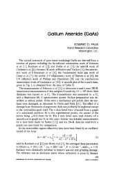
A2A-98-U-0-021 (APL)
EERL-98-12A (EERL)
December 1998
Handbook of
Propagation Effects for
Vehicular and Personal Mobile
Satellite Systems
Overview of Experimental and Modeling Results
Julius Goldhirsh *
and
Wolfhard J. Vogel #
* THE JOHNS HOPKINS UNIVERSITY, APPLIED PHYSICS LABORATORY
11100 JOHNS HOPKINS ROAD, LAUREL, MARYLAND 20723-6099
# THE UNIVERSITY OF TEXAS AT AUSTIN
ELECTRICAL ENGINEERING RESEARCH LABORATORY
10100 BURNET ROAD, AUSTIN, TEXAS 78758

Acknowledgements
This work was performed under JPL Contract No. 960204 for The Johns
Hopkins University, Applied Physics Laboratory and JPL Contract No.
956520 for The University of Texas at Austin, Electrical Engineering
Research Laboratory.

Table of Contents
1 Introduction _______________________________________________________ 1-4
1.1 Background _________________________________________________________ 1-4
1.2 Overview of Chapters in Revised Text ___________________________________ 1-5
1.3 Mobile Satellite Handbook on the Web___________________________________ 1-8
2 Attenuation Due to Trees: Static Case __________________________________ 2-1
2.1 Background _________________________________________________________ 2-1
2.2 Attenuation and Attenuation Coefficient at UHF___________________________ 2-1
2.3 Single Tree Attenuation at L-Band ______________________________________ 2-4
2.4 Attenuation through Vegetation: ITU-R Results ___________________________ 2-5
2.5 Distributions of Tree Attenuation at L-Band and K-Band ___________________ 2-6
2.6 Seasonal Effects on Path Attenuation ____________________________________ 2-8
2.7 Frequency Scaling Considerations______________________________________ 2-11
2.8 Conclusions and Recommendations_____________________________________ 2-15
2.9 References _________________________________________________________ 2-16
3 Attenuation Due to Roadside Trees: Mobile Case _________________________ 3-1
3.1 Background _________________________________________________________ 3-1
3.2 Time-Series Fade Measurements ________________________________________ 3-1
3.3 Extended Empirical Roadside Model ____________________________________ 3-4
3.4 Validation of the Extended Empirical Roadside Shadowing Model___________ 3-12
3.5 Attenuation Effects of Foliage _________________________________________ 3-19
3.6 Frequency Scaling Considerations______________________________________ 3-24
3.7 Comparison of EERS Model with Other Empirical Models _________________ 3-25
3.8 Conclusions and Model Recommendations_______________________________ 3-32
3.9 References _________________________________________________________ 3-33
4 Signal Degradation for Line-of-Sight Communications ____________________ 4-1
4.1 Background _________________________________________________________ 4-1
4.2 Multipath for a Canyon and Hilly Environments __________________________ 4-2
4.3 Multipath Due to Roadside Trees _______________________________________ 4-6
4.4 Multipath at 20 GHz Near Body of Water - Low Elevation Angle Effects ______ 4-8
4.5 Multipath Versus Driving Directions ___________________________________ 4-10
4.6 Empirical Multipath Model ___________________________________________ 4-13
4.7 Summary and Recommendations ______________________________________ 4-14
4.8 References _________________________________________________________ 4-15
5 Fade and Non-Fade Durations and Phase Spreads________________________ 5-1
5.1 Background _________________________________________________________ 5-1
5.2 Concept of Fade and Non-Fade Durations ________________________________ 5-1
5.3 Fade Durations Derived from Measurements in Australia ___________________ 5-3
5.4 Fade Duration Measurements in Central Maryland ________________________ 5-6
5.5 Fade Duration Distributions at Higher Elevation Angles ____________________ 5-7
i

5.6 Summary of Fade Duration Results______________________________________ 5-8
5.7 Cumulative Distributions of Non-Fade Durations: Australian Measurements__ 5-10
5.8 Cumulative Distributions of Non-Fade Duration: Central Maryland _________ 5-11
5.9 Cumulative Distributions of Phase Fluctuations: Australian Measurements ___ 5-11
5.10 Summary and Recommendations ____________________________________ 5-14
5.11 References _______________________________________________________ 5-14
6 Polarization, Antenna Gain and Diversity Considerations __________________ 6-1
6.1 Background _________________________________________________________ 6-1
6.2 Depolarization Effects_________________________________________________ 6-1
6.3 Distributions from Low- and High-Gain Receiving Antennas ________________ 6-2
6.4 Fade Reduction Due to Lane Diversity ___________________________________ 6-4
6.5 Antenna Separation Diversity Gain______________________________________ 6-7
6.6 Satellite Diversity____________________________________________________ 6-12
6.7 Conclusions and Recommendations_____________________________________ 6-16
6.8 References _________________________________________________________ 6-16
7 Investigations from Different Countries _________________________________ 7-1
7.1 Background _________________________________________________________ 7-1
7.2 Measurements in Australia_____________________________________________ 7-1
7.3 Belgium (PROSAT Experiment) ________________________________________ 7-6
7.4 Measurements in Canada ______________________________________________ 7-6
7.5 Measurements in England _____________________________________________ 7-8
7.6 France and Germany: European K-Band Campaign ______________________ 7-13
7.7 Measurements in Japan ______________________________________________ 7-14
7.8 Measurements Performed in the United States ___________________________ 7-16
7.9 Summary Comments and Recommendations_____________________________ 7-26
7.10 References _______________________________________________________ 7-27
8 Earth-Satellite Propagation Effects Inside Buildings ______________________ 8-1
8.1 Background _________________________________________________________ 8-1
8.2 Satellite Radio Reception Inside Buildings from 700 MHz to 1800 MHz________ 8-2
8.3 Slant-Path Building Penetration Measurements at L- and S-Band ___________ 8-12
8.4 Slant-Path Building Attenuation Measurements from 0.5 to 3 GHz __________ 8-21
8.5 Building Attenuation at UHF, L- and S-Band Via Earth-Satellite Measurements8-29
8.6 Attenuation of 900 MHz Radio Waves by Metal Building __________________ 8-31
8.7 Summary and Concluding Remarks ____________________________________ 8-31
8.8 References _________________________________________________________ 8-34
9 Maritime-Mobile Satellite Propagation Effects ___________________________ 9-1
9.1 Introduction _________________________________________________________ 9-1
9.2 Early Multipath Experiments __________________________________________ 9-1
9.3 Characteristics of Multipath Fading Due to Sea Surface Reflection ___________ 9-3
9.4 Model of Fade Durations Due to Sea Reflections __________________________ 9-13
9.5 Multipath from Rough Seas and Frequency Dependence on Multipath Fading_ 9-20
9.6 Other Maritime Investigations_________________________________________ 9-22
9.7 Summary and Recommendations ______________________________________ 9-23
9.8 References _________________________________________________________ 9-24
ii

10 Optical Methods for Assessing Fade Margins ___________________________ 10-1
10.1 Background ______________________________________________________ 10-1
10.2 General Methodology ______________________________________________ 10-2
10.3 Skyline Statistics of Austin and San Antonio, Texas _____________________ 10-3
10.4 Clear, Shadowed and Blocked Propagation States ______________________ 10-5
10.5 Urban Three-State Fade Model (UTSFM) _____________________________ 10-8
10.6 Estimation of Urban Fading for the Globalstar Constellation _____________ 10-9
10.7 Statistics of Potentially Visible Satellites in Various States_______________ 10-11
10.8 Satellite Diversity ________________________________________________ 10-13
10.9 Summary Comments and Recommendations__________________________ 10-17
10.10 References ______________________________________________________ 10-18
11 Theoretical Modeling Considerations__________________________________ 11-1
11.1 Background ______________________________________________________ 11-1
11.2 Background Information Associated with Model Development____________ 11-2
11.3 Empirical Regression Models________________________________________ 11-4
11.4 Probability Distribution Models ____________________________________ 11-10
11.5 Geometric Analytic Models ________________________________________ 11-23
11.6 Summary and Recommendations ___________________________________ 11-30
11.7 References ______________________________________________________ 11-31
12 Summary of Recommendations_______________________________________ 12-1
12.1 Introduction (Chapter 1) ___________________________________________ 12-1
12.2 Average Foliage Attenuation Due to Trees: Static Case (Chapter 2)________ 12-1
12.3 Attenuation Due to Roadside Trees: Mobile Case (Chapter 3)_____________ 12-2
12.4 Signal Degradation for Line-of-Sight Communications (Chapter 4) ________ 12-5
12.5 Fade and Non-Fade Durations and Phase Spreads (Chapter 5)____________ 12-6
12.6 Polarization, Antenna Gain and Diversity Considerations (Chapter 6) _____ 12-8
12.7 Investigations from Different Countries (Chapter 7) ___________________ 12-11
12.8 Earth-Satellite Propagation Effects Inside Buildings (Chapter 8) _________ 12-13
12.9 Maritime-Mobile Satellite Propagation Effects (Chapter 9)______________ 12-15
12.10 Optical Methods for Assessing Fade Margins for Shadowing, Blockage, and Clear
Line-of-Sight Conditions (Chapter 10)______________________________________ 12-18
12.11 Theoretical Modeling Considerations (Chapter 11) ____________________ 12-20
Index
iii

Chapter 1
Introduction

Table of Contents
1 Introduction ________________________________________________________ 1-1
1.1 Background _________________________________________________________ 1-1
1.2 Overview of Chapters in Revised Text ___________________________________ 1-1
1.2.1 Chapter 2: Attenuation Due to Trees: Static Case _______________________________ 1-1
1.2.2 Chapter 3: Attenuation Due to Roadside Trees: Mobile Case ______________________ 1-2
1.2.3 Chapter 4: Signal Degradation for Line-of-Sight Communications _________________ 1-2
1.2.4 Chapter 5: Fade and Non-Fade Durations and Phase Spreads______________________ 1-3
1.2.5 Chapter 6: Polarization, Antenna Gain, and Diversity Considerations _______________ 1-3
1.2.6 Chapter 7: Investigations from Different Countries _____________________________ 1-3
1.2.7 Chapter 8: Earth-Satellite Propagation Effects Inside Buildings (NEW)_______________ 1-3
1.2.8 Chapter 9: Maritime-Mobile Satellite Propagation Effects (NEW) ___________________ 1-4
1.2.9 Chapter 10: Optical Methods for Assessing Fade Margins for Shadowing, Blockage and
Clear Line-of-Sight Conditions (NEW) _______________________________________________ 1-4
1.2.10 Chapter 11: Theoretical Modeling Considerations ______________________________ 1-4
1.2.11 Chapter 12: Recommendations for Further Investigations ________________________ 1-5
1.3 Mobile Satellite Handbook on the Web___________________________________ 1-5
1.3.1 Contents on the Home Page________________________________________________ 1-5
1.3.2 From Table of Contents to Viewing a Chapter Text _____________________________ 1-6
1.3.3 Downloading a Chapter into a PDF File for Printout or Saving into a File____________ 1-6
1.3.4 Communicating with the Authors ___________________________________________ 1-6
1-i

Chapter 1
Introduction
1.1 Background
This handbook is a revision of NASA Reference Publication 1274 entitled, “Propagation
Effects for Land Mobile Satellite Systems: Overview of Experimental and Modeling
Results,” by Goldhirsh and Vogel. The revised text contains pertinent features of the
original document plus updates of experiments and models available since 1992 dealing
with propagation effects for earth-satellite scenarios. Additional topics that have reached
an appropriate level of maturity are also described. These include optical means to
establish propagation statistics, propagation effects on satellite paths reaching inside
buildings and marine-satellite propagation. To streamline the reading and the acquisition
of information, each chapter contains its own table of contents, table of figures, listing of
tables, recommendations, and references. The chapters are written such that they are selfcontained
requiring little or no searching for information in other chapters. The
following paragraphs give a brief overview of the contents of each of the chapters with
new information denoted by (NEW). Also presented is a step-by-step procedure for
accessing this text on the World Wide Web and interacting with the authors.
1.2 Overview of Chapters in Revised Text
1.2.1 Chapter 2: Attenuation Due to Trees: Static Case
This chapter deals with propagation effects caused by trees derived from stationary
measurements. It presents values of attenuation coefficients and path attenuations
associated with single trees of different “types.” Largest and average values measured
are given for frequencies at UHF (870 MHz) and L-Band (1.6 GHz). Plots of attenuation
coefficient versus frequency are presented covering the frequency range of 30 MHz
through 3 GHz corresponding to ground-to-ground measurements through woodland,
forest or jungle over paths of 100 m or more (NEW). Cumulative distributions of
attenuation at L-Band and K-Band (19.6 GHz) are presented for Pecan trees “with” and

1-2
Propagation Effects for Vehicular and Personal Mobile Satellite Systems
“without” leaves (NEW). Formulations are presented giving the attenuation versus
elevation angle at UHF (870 MHz) and L-Band with and without leaves. Frequency
scaling formulations are given for intervals between UHF (870 MHz) and L-Band,
L-Band (1 GHz) and S-Band (4 GHz), and L-Band (1.6 GHz) and K-Band (19.6 GHz)
(NEW).
1.2.2 Chapter 3: Attenuation Due to Roadside Trees: Mobile Case
Measurements and empirical models are examined in this chapter for earth-satellite
scenarios in which a vehicle is driven along tree-lined roads and where the signal
degradation is primarily due to attenuation from tree canopies. Examples of time-series
of attenuation and phase at L-Band (1.5 GHz) and K-Band (20 GHz) are presented (NEW).
An Extended Empirical Roadside Shadowing model is characterized with a step-by-step
procedure for implementation (NEW). This model was adopted by the International
Telecommunication Union Radio Communication Sector (ITU-R). It extends the
previous empirical roadside shadowing model as follows: (1) It provides frequency
scaling from UHF (870 MHz) to K-Band (20 GHz), (2) it enables elevation angle scaling
from 7° to 80°, and (3) it may be applied to percentage ranges from 1% to 80%.
Probability distributions of attenuations for measurements in Central Maryland,
Australia, Texas, Washington State, and Alaska are compared with the distributions
derived from the EERS model (NEW). Comparisons are also made with measurements
made by the European Space Agency (ESA) (NEW). An equal probability formulation for
attenuation by trees with and without foliage at K-Band (20 GHz) is presented and
validated using an independent set of measurements (NEW). Other empirical models are
presented and compared with the EERS model (NEW). These include the Modified
Empirical Roadside Shadowing (MERS), Empirical Fading Model (EFM), and the
Combined Empirical Fading Model (CEFM). An examination of the ITU-R Fade Model
at elevations above 60° is also examined (NEW).
1.2.3 Chapter 4: Signal Degradation for Line-of-Sight Communications
Mobile satellite signal degradation is examined for a geometry in which line-of-sight
communications are maintained with minimal shadowing and where signal variability is
due to multipath from the ground, roadside trees, utility poles, hills, mountains, or a
nearby body of water. Cumulative distribution models are given for canyon
measurements at UHF (870 MHz) and L-Band (1.5 GHz) at elevations of 30° and 45°,
hilly environments at L-Band at elevations of 7° to 14° (NEW), and roadside trees at UHF
and L-Band at 30°, 45°, and 60°. Cumulative fade distributions at K-Band (20 GHz)
associated with multipath due to reflections from a nearby body of water and from dry
land at 8° elevation for various vehicle orientations are described (NEW). Cumulative
fade distributions at K-Band (20 GHz and 18.7 GHz) due to multipath for various
pointing aspects relative to the satellite location and tree-line geometries are given (NEW).
An empirical multipath model of the cumulative fade distribution was developed
representing the median of 12 multipath distributions at frequencies from 870 MHz to
20 GHz and elevation angles from 8° to 60° (NEW). The model covers a percentage range
of 1% to 50%.

Introduction 1-3
1.2.4 Chapter 5: Fade and Non-Fade Durations and Phase Spreads
Fade duration distributions for tree-lined roads at L-Band (1.5 GHz) are presented.
Dependence of fade duration distributions at L-Band on elevation angle for
measurements in the United States and Europe are described (NEW). The ITU-R model
describing the cumulative distribution of fade duration is given and compared with
measurements (NEW). Non-fade durations for tree-lined road scenarios are characterized
for L-Band. Dependence of non-fade duration distributions as a function of elevation
angle is examined (NEW). Phase fluctuation distributions for “moderate” and “extreme”
shadowing” conditions are presented and a corresponding model is given.
1.2.5 Chapter 6: Polarization, Antenna Gain, and Diversity Considerations
Fade effects at L-Band (1.5 GHz) and UHF (870 MHz) are related to depolarization,
antenna gain, lane changing, antenna space diversity, and satellite path diversity (NEW).
A curve and corresponding formulation describing the cross-polarization isolation at
L-Band (1.5 GHz) versus the co-polarization fade level is presented for a roadside tree
environment. An example describing the effects on fade distributions is reviewed when
high and low gain antennas are used for a tree-lined environment. The effects of fade
reduction (or enhancement) achieved by “changing lanes” are described and a “fadereduction”
formulation is given for elevation angles of 30°, 45°, and 60° for UHF
(870 MHz) and L-Band (1.5 GHz). A model for diversity improvement factor is
presented at L-Band (1.5 GHz). (This quantity is the ratio of the single terminal
probability to the joint probability for a given spacing at a given fade margin.) Diversity
gain (tree-lined roads) versus antenna spacing from 1 to 10 m is presented. Diversity
gains at L-Band for expressway driving in Japan for antenna separations of 5 m and 10 m
are reviewed (NEW). Single and joint fade distributions are presented associated with
switching communications to different satellites in a given constellation such that smaller
fading is experienced (NEW). These satellite diversity distributions were based on
simulations employing optical measurements of the skyline. Direct satellite diversity
measurements of single and joint fading distributions at S-Band (2 GHz) employing
NASA’s Tracking and Data Relay Satellite System (TDRSS) are described (NEW).
1.2.6 Chapter 7: Investigations from Different Countries
A compendium of measured cumulative fade distributions for Land-Mobile-Satellite
System (LMSS) is presented. The different measurement campaigns’ frequency,
elevation angle, 1% and 10% fades, environment, and associated reference is tabulated
(NEW). A brief background description associated with each of these measurements is
given and the corresponding cumulative fade distributions are presented for frequencies
of UHF (870 MHz) through K-Band (20 GHz) and elevation angles from 8° to 80° (NEW).
1.2.7 Chapter 8: Earth-Satellite Propagation Effects Inside Buildings (NEW)
This new chapter describes propagation effects for the case in which transmissions
originate from a satellite and receiver measurements are made inside various building
types. Relative signal losses associated with spatial, temporal, and frequency intervals
are described. Signal level variation with frequency is characterized over a frequency

1-4
Propagation Effects for Vehicular and Personal Mobile Satellite Systems
interval of 700 MHz to 1.8 GHz, 1.6 GHz, and 2.5 GHz. Cumulative fade distributions at
these frequencies are characterized. The efficacy of space and frequency diversity
interior to buildings is examined. Bandwidth distortion is considered.
1.2.8 Chapter 9: Maritime-Mobile Satellite Propagation Effects (NEW)
Multipath fading from the ocean is characterized when low gain antennas are used for
low-elevation angle marine-satellite scenarios. An overview of early multipath ship-tosatellite
fade measurements at various frequencies ranging from 240 MHz to 30 GHz is
reviewed. Characteristics of specular and diffuse multipath fading due to sea surface
reflections are examined. Models are presented giving the fading depth versus the
elevation angle at various probability levels. Fade duration models are also presented.
Dependence of the model values on significant wave height and frequencies ranging from
1 GHz to 10 GHz is examined.
1.2.9 Chapter 10: Optical Methods for Assessing Fade Margins for Shadowing,
Blockage and Clear Line-of-Sight Conditions (NEW)
This new chapter deals with single and joint earth-satellite fade distributions derived from
the photographing of roadside images of the skyline and analyzing the ambient scene in
terms of (1) clear line-of-sight with multipath reflections, (2) shadowed state, and (3)
blocked state. The general methodology of making such measurements is described and
examples of skyline statistics are presented. The formulations for “clear,” shadowed,”
and “blocked” propagation states are presented. Parameter values for earth-satellite
measurements at L-Band (1.5 GHz) for urban Japan are given. Cumulative fade
distributions are derived from these formulations and compared with a measured
distribution. Probability distributions for a series of elevation angles are presented for
elevation angles ranging from 7° to 82°. Single and joint cumulative fade distributions
are derived from a simulated constellation of satellites for urban areas of London, Tokyo,
and Singapore. Statistics of potentially visible satellites in various states given a
constellation are derived. Diversity gains are derived for “combining” and “handoff”
diversity modes.
1.2.10 Chapter 11: Theoretical Modeling Considerations
In this chapter are reviewed the elements of diffuse and specular scattering. Density
functions used in propagation modeling are examined. These include Nakagami-Rice,
Rayleigh, and lognormal density functions. The theoretical models examined are (1) Loo
Distribution, (2) Lutz Total Shadowing Model, (3) Lognormal Shadowing, and (4)
Simplified Lognormal Shadowing. Models are also considered associated with “fade
state transitions.” In particular, 2-state and 4-state Markov models are characterized.
Geometric analytic models associated with signal and multiple point scatterers are
presented. Recommendations regarding the efficacy of each of the models are made
throughout the chapter.

Introduction 1-5
1.2.11 Chapter 12: Recommendations for Further Investigations
In this chapter are reviewed the gaps in our understanding of propagation effects vis-à-vis
present and projected scenarios for mobile-satellite scenarios. These scenarios include
land (mobile and personal), marine, and aeronautical to satellite scenarios for
geostationary and orbiting constellations. Recommendations are made for further
investigations to fill the indicated gaps.
1.3 Mobile Satellite Handbook on the Web
It is the author’s intention to make this handbook fully accessible via the World Wide
Web, both as a service to the users, but also to facilitate feedback for improvements and
revisions.
A step-by-step procedure is provided for accessing the individual handbook chapters
already on the world-wide-web, downloading these chapters onto your personal
computer, printing them in a paper format and saving them to a file. As mentioned, this
handbook is a revision of NASA Reference Publication 1274 that may be also accessed
and downloaded from the “home” page whose address is given in the following
paragraph.
1.3.1 Contents of the Home Page
The “home page” may be attained after dialing the web address
http://www.utexas.edu/research/mopro/index.html titled “Propagation Effects/MSS.”
The home page contains linkages to a number of locations. From top to bottom, these
include
• Home pages of NASA, APL, EERL, and JPL by clicking appropriate icon
• Submission of e-mail messages to the authors by clicking e-mail addresses under
the individual author’s name
• Previous publication (NASA Reference Publication 1274) obtained by clicking
the blue report at center-left
• Table of contents of revised document by clicking “Table of Contents,”
• Glossary of terms and abbreviations (under construction) by clicking “Glossary
of Terms and Abbreviations,”
• Paper copy of individual chapters obtained by clicking “How to Get a Paper
Copy,”
• Submittal of your comments to authors by clicking “Your Feedback,” and
• A short biography of the authors by clicking “The Authors.”

1-6
Propagation Effects for Vehicular and Personal Mobile Satellite Systems
1.3.2 From Table of Contents to Viewing a Chapter Text
Clicking “Table of Contents” links the user to a listing of chapters. The chapter titles
displayed as links are those available on the web and ready for downloading. Clicking on
the title link may access the Table of Contents for any particular chapter. As an example,
by clicking on Chapter 10 (Optical Methods for Assessing Fade Margins), we link to the
corresponding Table of Contents for Chapter 10. Any of the chapter sections listed in the
table of contents may be viewed by clicking on the desired section title. For example,
clicking the title for Section 10.2 (General Methodology) links only to this section, which
may be saved or printed. One may also link to a particular figure or reference by clicking
on a particular figure number or reference (shown as link). For example, clicking on
“Figure 10.1” results in the display of Figure 10.1, and clicking on the reference “Vogel
and Hong, 1988” links to the corresponding entry in the list of references. Both the
figure and the listing of references are capable of being printed out in this mode.
1.3.3 Downloading a Chapter into a PDF File for Printout or Saving into a File
One may download an Adobe PDF version of each chapter for off-line browsing or
printing by clicking “How to Get a Paper Copy” in the home page. This will link to
another page enabling you to download the Adobe Acrobat software. Assuming Acrobat
is already loaded onto the personal computer, one may download Chapter 10 (for
example) by clicking on its chapter title. After the chapter is downloaded, it may be
printed or saved to a file in your personal computer.
1.3.4 Communicating with the Authors
The reader may send a message to the authors by clicking “Your Feedback” or by
clicking the authors email addresses given as links at the top of the home page. The
authors encourage comments regarding errors in the text or suggested subjects to be
included in a follow-up edition of this handbook.

Chapter 2
Attenuation Due to Trees:
Static Case

Table of Contents
2 Attenuation Due to Trees: Static Case ___________________________________ 2-1
2.1 Background _________________________________________________________ 2-1
2.2 Attenuation and Attenuation Coefficient at UHF___________________________ 2-2
2.3 Single Tree Attenuation at L-Band ______________________________________ 2-4
2.4 Attenuation through Vegetation: ITU-R Results ___________________________ 2-5
2.5 Distributions of Tree Attenuation at L-Band and K-Band ___________________ 2-6
2.6 Seasonal Effects on Path Attenuation ____________________________________ 2-8
2.6.1 Effects of Foliage at UHF _________________________________________________ 2-8
2.6.2 Effects of Foliage at L-Band ______________________________________________ 2-10
2.6.3 Effects of Foliage at K-Band ______________________________________________ 2-10
2.7 Frequency Scaling Considerations______________________________________ 2-11
2.7.1 Scaling between 870 MHz and L-Band______________________________________ 2-11
2.7.2 Scaling between 1 GHz and 4 GHz _________________________________________ 2-12
2.7.3 Scaling between L-Band and K-Band _______________________________________ 2-14
2.8 Conclusions and Recommendations_____________________________________ 2-15
2.9 References _________________________________________________________ 2-16
Table of Figures
Figure 2-1: LMSS propagation path shadowed by the canopies of one or two trees in which the
attenuation path length is relatively well defined. .......................................................................... 2-1
Figure 2-2: Low elevation propagation through a grove of trees giving rise to ambiguity in
attenuation path length.................................................................................................................. 2-2
Figure 2-3: Attenuation coefficients as described by the ITU-R for both "short paths” (square
points) and "long path" (solid and dashed lines and diamond point at 10 GHz) scenarios. .............. 2-6
Figure 2-4: Cumulative distributions at L-Band (1.6 GHz) and K-Band (19.6 GHz). The cases
considered are: (A) K-Band Pecan in leaf, (B) K-Band Magnolia (evergreen), (C) K-Band
Pecan without leaves, (D) L-Band Pecan in leaf, (E) L-Band Pecan without leaves, (F) K-Band
unobstructed line-of-sight............................................................................................................. 2-7
Figure 2-5: Configuration showing the approximate dimensions of the Callery Pear tree and the
relative location of the receiver. All dimensions are expressed in meters....................................... 2-8
Figure 2-6: Static tree attenuation versus elevation angle at 870 MHz for the Callery Pear tree
configuration in Figure 2-5. Triangles represent the full-foliage case, diamonds the no-foliage
case.............................................................................................................................................. 2-9
Figure 2-7: Comparison of measured (solid curves) and predicted (dashed) attenuation distributions
at 19.6 GHz corresponding to foliage and non-foliage cases. ....................................................... 2-12
2-i

Figure 2-8: Ratio of Attenuations versus frequency using different frequency scaling criteria
normalized to 1 GHz. The solid curve corresponds to (2-7), the dashed curve to (2-8) and the
dot-dashed curve to (2-9)............................................................................................................ 2-13
Figure 2-9: Frequency scaling of attenuation distribution of measured L-Band (1.6 GHz) to S-Band
frequencies using different criteria. Also shown is measured S-Band distribution........................ 2-13
Figure 2-10: Cumulative distributions at L (1.6 GHz; curve A) and K (19.6 GHz curve B) derived
from measurements. Curves C, D, and E are the frequency scaled distributions (L to K)
derived employing (2-9), (2-7), and (2-8), respectively................................................................ 2-15
Table of Tables
Table 2-1: Summary of Single Tree Attenuations at f = 870 MHz.........................................................2-3
Table 2-2: Attenuation coefficient and average attenuations at 1.6 GHz of the different tree types..........2-5
Table 2-3: Median and 1% attenuation and attenuation coefficients at K- and L-Band............................2-7
2-ii

Chapter 2
Attenuation Due to Trees: Static Case
2.1 Background
A typical scenario in which fading occurs is depicted in Figure 2-1, which shows a
vehicle receiving satellite transmissions. The vehicle, which has an antenna mounted on
its roof, is presumed to be at a distance of 10 to 20 m from the roadside trees, and the
path to the satellite is generally above 20° in elevation. The antenna is to some extent
directive in elevation such that multipath from lower elevation (i.e., near zero degrees and
below) is filtered out by the antenna gain pattern characteristics. Although there may
exist multipath contributions at various azimuths, shadowing from the canopies of one or
two trees give rise to the major attenuation contributions. That is, the signal fade for this
case is due primarily to scattering and absorption from both branches and foliage where
the attenuation path length is the interval within the first few Fresnel zones intersected by
the canopies.
Figure 2-1: LMSS propagation path shadowed by the canopies of one or two trees in
which the attenuation path length is relatively well defined.
This geometry is in contrast to the configuration in which the transmitter and receiver are
located near the ground and propagation takes place through a grove of trees as shown in

2-2
Propagation Effects for Vehicular and Personal Mobile Satellite Systems
Figure 2-2. The attenuation contribution for this configuration is a manifestation of the
combined absorption and multiple scattering from the conglomeration of tree canopies
and trunks. For this case, an estimation of the attenuation coefficient from attenuation
measurements requires knowledge of the path length usually estimated to be the “grove
thickness.” This thickness may encompass a proportionately large interval of nonattenuating
space between the trees. Hence attenuation coefficients as derived for groves
of trees may underestimate the attenuation coefficient vis-à-vis those derived for path
lengths intersecting one or two contiguous canopies for LMSS scenarios as shown in
Figure 2-1. This chapter deals primarily with characterizing the path attenuation through
tree canopies pertaining to the scenario of Figure 2-1, although attenuation coefficients
associated with that of Figure 2-2 are briefly characterized in Section 2.4.
Figure 2-2: Low elevation propagation through a grove of trees giving rise to ambiguity
in attenuation path length.
Static measurements of attenuation due to isolated trees for LMSS configurations have
been systematically performed at UHF, L-Band, S-Band and or K-Band by Benzair et al.
[1991], Butterworth [1984a; 1984b], Cavdar et al. [1994], Vogel and Goldhirsh [1994;
1993; 1986], Vogel et al. [1995], Ulaby et al. [1990], and Yoshikawa and Kagohara
[1989].
2.2 Attenuation and Attenuation Coefficient at UHF
For those cases in which shadowing dominates, the attenuation primarily depends on the
path length through the canopy, and the density of foliage and branches in the first
Fresnel region along the line-of-sight path. The receiver antenna pattern may also
influence the extent of fading or signal enhancements via the mechanism of multipath
scattering from surrounding trees or nearby illuminated terrain. An azimuthally omnidirectional
antenna is more susceptible to such multipath scattering than a directive
antenna. Nevertheless, the authors found through measurements and modeling
considerations for LMSS scenarios, the major fading effects are a result of the extent of
shadowing along the line-of-sight direction.
In Table 2-1 is given a summary of the single tree attenuation results at 870 MHz
based on the measurements by the authors [Vogel and Goldhirsh, 1986; Goldhirsh and
Vogel, 1987] who employed remotely piloted aircraft and helicopter transmitter
platforms. The attenuations were calculated by comparing the power changes for a
configuration in which the receiving antenna (on the roof of a van) was “in front of” and

Attenuation Due to Trees: Static Case 2-3
“behind” a particular tree. The former and latter cases offered non-shadowed and
maximum shadowing conditions, respectively, relative to the line of sight propagation
path from the transmitter on the aircraft to the stationary receiver. During each flyby, the
signal levels as a function of time were expressed in terms of a series of median fades
derived from the 1024 samples measured over one second periods. The attenuation
assigned to the particular flyby was the highest median fade level observed at the
measured elevation angle. It may be deduced that the motion of the transmitter aperture
and the receiver’s sampling rate of 1024 samples per second resulted in more than 200
independent samples averaged each second. This sample size is normally adequate to
provide a well-defined average of a noisy signal. The individual samples from which the
median was derived over the one-second period were observed to fluctuate on the
average ±2 dB about the median due to the influence of variable shadowing and
multipath.
Table 2-1: Summary of Single Tree Attenuations at f = 870 MHz.
Tree Type
Attenuation (dB) Attenuation Coefficient (dB/m)
Largest Average Largest Average
Burr Oak* 13.9 11.1 1.0 0.8
Callery Pear 18.4 10.6 1.7 1.0
Holly* 19.9 12.1 2.3 1.2
Norway Maple 10.8 10.0 3.5 3.2
Pin Oak 8.4 6.3 0.85 0.6
Pin Oak* 18.4 13.1 1.85 1.3
Pine Grove 17.2 15.4 1.3 1.1
Sassafras 16.1 9.8 3.2 1.9
Scotch Pine 7.7 6.6 0.9 0.7
White Pine* 12.1 10.6 1.5 1.2
Average 14.3 10.6 1.8 1.3
RMS 4.15 2.6 0.9 0.7
The first column in Table 2-1 lists the trees examined where the presence of an asterisk
corresponds to results of measurements at Wallops Island, VA in June 1985 (remotely
piloted aircraft), and the absence of the asterisk represents measurements in central MD
in October 1985 (helicopter). During both measurement periods, the trees examined were
approximately in full foliage conditions. The second and third columns labeled “Largest”
and “Average” represent the largest and average values, respectively, of attenuation (in
dB) derived for the sum total of flybys for that particular tree. The fourth and fifth
columns denote the corresponding attenuation coefficients derived from the path length
through the canopy. The path length was estimated from measurements of the elevation
angle, the tree dimensions, and the relative geometry between the tree and the receiving
antenna height. The dependence of the attenuation on elevation angle is described in
Section 2.6. We note that the attenuations from Pin Oak as measured at Wallops Island
(with asterisk) is significantly larger than that measured in central Maryland (without

2-4
Propagation Effects for Vehicular and Personal Mobile Satellite Systems
asterisk) because the former tree had a significantly greater density of foliage over
approximately the same path length interval. This result demonstrates that a description
of the attenuation from trees for LMSS scenarios may only be handled employing
statistical processes.
Butterworth [1984b] performed single tree fade measurements at 800 MHz
(circularly polarized transmissions) at seven sites in Ottawa, Canada over the path
elevation interval 15 o to 20 o . The transmitter was located on a tower and receiver
measurements were taken at a height of 0.6 m above the ground. Measurements were
performed from April 28 to November 4, 1981 covering the period when leaf buds started
to open until after the leaves had fallen from the trees. A cumulative distribution of
foliage attenuation readings covering a 19 day period in June 1981 was noted to be
lognormal, where the fades exceeded 3 and 17 dB for 80% and 1% of the measured
samples, respectively. The median attenuation was approximately 7 dB with an
approximate median attenuation coefficient of 0.3 dB/m (24 m mean foliage depth). The
average attenuation coefficient of Butterworth is smaller than those measured by the
authors in central Maryland and Virginia. The disparity between these results may be
due to differences in the methods of averaging, the heights of the receiver and the
interpretation of the shadowing path length as previously described.
2.3 Single Tree Attenuation at L-Band
Single tree attenuation measurements at 1.6 GHz were conducted in Turkey between
April and September of 1993 by Cavdar et al. [1994]. The transmitter was placed atop a
building and the receiver antenna was located on top of a mobile unit which positioned
itself at different locations in the shadowed region of a number of trees.
Table 2-2 gives the total path attenuation and attenuation coefficients for a series of
trees. The average attenuation and attenuation coefficient are similar at UHF (Table 2-1)
to their respective values at L-Band (Table 2-2), although their respective RMS values
are significantly different.

Attenuation Due to Trees: Static Case 2-5
Table 2-2: Attenuation coefficient and average attenuations at 1.6 GHz of the different
tree types.
Tree Type
Average
Attenuation (dB)
Attenuation
Coefficient
(dB/m)
Willow 10.45 1.1
Pine 18.0 1.8
Linden 9.1 1.4
European Alder 7.0 1.0
Acacia 6.75 0.9
Poplar 3.5 0.7
Elm 9.0 1.2
Hazelnut 2.75 1.1
Maple 16.25 1.25
White Spruce 20.1 1.75
Laurel Cherry 12.0 2.0
Plane 16.9 1.35
Fir 12.75 1.5
Fruit 9.6 1.2
Average 11.0 1.3
RMS 5.1 0.35
2.4 Attenuation through Vegetation: ITU-R Results
The ITU-R [1994] designates attenuation through vegetation in terms of ground-toground
measurements over paths of approximately 100 m or more, in woodland, forest or
jungle with antenna heights of 2-3 m above the ground with only part of the ray passing
through the foliage as designated in Figure 2-2. Attenuation corresponding to this
scenario is referred to as “long path.” A “short-path attenuation” scenario is also
designated corresponding to short ground-to-ground or slant-path measurements through
the foliage of individual trees with foliage depths of no more than 10-15 m as shown in
Figure 2-1. Figure 2-3 gives the attenuation coefficient in dB/m versus frequency for
both the short-path (squares) and long-path (solid and dashed curves and diamond at
approximately 10 GHz). As mentioned, the long-path results show attenuation
coefficients significantly smaller than the short path results. Short-path attenuation
coefficients between 1 and 2 dB/m are generally indicated at frequencies between
approximately 1 and 4 GHz consistent with the results of Table 2-1 and Table 2-2.

2-6
Attenuation Coefficient (dB/m)
1E+1
8
6
4
2
1E+0
8
6
4
2
1E-1
8
6
4
2
1E-2
8
6
4
1E-3
2
Short Path Data
V
H
Propagation Effects for Vehicular and Personal Mobile Satellite Systems
Long Path
2 4 6 8 2 4 6 8 2 4 6 8 2 4 6 8
1E+1 1E+2 1E+3 1E+4 1E+5
Frequency (MHz)
Figure 2-3: Attenuation coefficients as described by the ITU-R for both "short paths”
(square points) and "long path" (solid and dashed lines and diamond point at 10 GHz)
scenarios.
2.5 Distributions of Tree Attenuation at L-Band and K-Band
Static tree attenuation measurements at L- (1.6 GHz) and K-Band (19.6 GHz) were
executed in Austin, Texas [Vogel and Goldhirsh, 1993; 1994]. The trees sampled were
Pecan (deciduous) and Magnolia (evergreen). The L-Band measurements were
performed in December 1990 and July 1991 during which times the sampled Pecan tree
was “without foliage” and in “full foliage,” respectively. The transmitter was placed atop
a 20 m tall tower and the receiving antenna was mounted on a motorized positioner
placed within the geometric shadow zone of each tree. The antenna was moved slowly
over a horizontal distance of several meters, and the received power was sampled every
0.1 s for about 100 s. The K-Band measurements were performed in March and May,
1993 employing the same approximate geometry. These months also correspond to
periods in which the Pecan tree was without leaves and in full foliage, respectively. The
receiving antenna was hand-held and moved horizontally over a distance of several
meters, first in the shadow of the same Pecan tree, and then in the shadow of the nearby
Magnolia tree. Quadrature detector receiver voltages were sampled at a 1000 Hz rate for
several minutes. The path lengths within the Pecan and Magnolia crowns were on
average 9 m and 4.5 m, respectively. The clear line-of-sight reference signal levels were
determined for all cases by moving the receiver to an equi-distant position where the
signal path was unobstructed.

Attenuation Due to Trees: Static Case 2-7
Resulting cumulative fade distributions are given in Figure 2-4 for cases in which
the canopy optically shadowed the line-of-sight path between the transmitter and the
receiver (curves A through E). Also given, as a reference, is the distribution for the
unobstructed K-Band line-of-sight case (curve F). In Table 2-3 is given a summary of the
total attenuation and attenuation coefficient for the median (50%) and 1% cases for the
different frequencies and tree scenarios characterized in Figure 2-4. The elevation angles
for the K and L-Band measurements relative to the Pecan tree were approximately 26°
and 30°, respectively.
Table 2-3: Median and 1% attenuation and attenuation coefficients at K- and L-Band.
Tree Condition Percentage
Percentage of Locations >Abscissa
Clear LOS Median 0.5
Total Fade (dB) Attenuation Coefficient (dB/m)
L-Band K-Band L-Band K-Band
1% 2.6
Bare Pecan Median 10.3 6.9 1.1 0.75
1% 18.4 25.0 2.0 2.8
Pecan in leaf Median 11.6 22.7 1.3 2.5
1% 18.6 43.0 2.1 4.8
Magnolia Median 19.6 4.4
(evergreen) 1% 39.6 8.8
100
9
8
7
6
5
4
3
2
10
9
8
7
6
1
5
4
3
2
F
E
D
C
0 5 10 15 20 25 30 35 40
Fade (dB)
Figure 2-4: Cumulative distributions at L-Band (1.6 GHz) and K-Band (19.6 GHz). The
cases considered are: (A) K-Band Pecan in leaf, (B) K-Band Magnolia (evergreen),
(C) K-Band Pecan without leaves, (D) L-Band Pecan in leaf, (E) L-Band Pecan without
leaves, (F) K-Band unobstructed line-of-sight
B
A

2-8
2.6 Seasonal Effects on Path Attenuation
2.6.1 Effects of Foliage at UHF
Propagation Effects for Vehicular and Personal Mobile Satellite Systems
It is observed from the configuration of Figure 2-1, that at smaller elevation angles, the
path length through the canopy will increase. Likewise, it is expected that the attenuation
will also increase assuming the path cuts through the canopy. Single tree attenuation
measurements for 870 MHz at different elevation angles were performed in central-
Maryland in October 1985 and in March 1986 for a Callery Pear tree employing a
helicopter as the transmitter platform [Goldhirsh and Vogel, 1987]. The approximate
geometry of the tree and relative location of the receiving antenna is given in Figure 2-5.
Figure 2-6 shows the corresponding results for the two seasons during which the tree was
in full foliage (October) and without leaves (March). Also shown are the linear fits for
each of the sets of data points.
Antenna
Position
2.4
17.6
6.6
11.2
13.8
2
45 °
To Helicopter
30 °
Figure 2-5: Configuration showing the approximate dimensions of the Callery Pear tree
and the relative location of the receiver. All dimensions are expressed in meters.

Attenuation Due to Trees: Static Case 2-9
Tree Attenuation (dB)
20
18
16
14
12
10
8
6
4
2
0
0 5 10 15 20 25 30 35 40 45
Path Elevation Angle (deg)
Figure 2-6: Static tree attenuation versus elevation angle at 870 MHz for the Callery Pear
tree configuration in Figure 2-5. Triangles represent the full-foliage case, diamonds the
no-foliage case.
The linear best fits in Figure 2-6 may be described as follows:
for 15 o < θ

2-10
Propagation Effects for Vehicular and Personal Mobile Satellite Systems
This results suggests that the predominant attenuation at 870 MHz arises from the tree
branches via the mechanism of absorption and the scattering of energy away from the
receiver. The conclusion that the wood part of the tree is the major contributor to
attenuation has also been substantiated at UHF for the mobile case (Chapter 3). The
above results are limited to elevation angles above approximately 15°. At smaller angles,
the path may pass through the bottom part of the canopy. More complicated scenarios
may result in which there may be multiple tree effects as depicted in Figure 2-2 or terrain
blockage may arise. The lower angle limit for mobile scenarios is broached in Chapter 3.
2.6.2 Effects of Foliage at L-Band
Upon analyzing the data points at equal probability levels for the L-Band distributions
with and without foliage (curves D and E of Figure 2-4), we observed that the percent
difference in fades between the foliage relative to the no-foliage cases for the Pecan tree
ranged from approximately 15% at 70% probability to 1% at 1% probability with an
average percent difference of approximately 7% (average fade difference = 0.8 dB). The
linear least square relation with a standard error of 0.1 dB relating the attenuation with
foliage to that with no foliage is given by,
for 9 dB < A(no foliage) < 18 dB
A ( full foliage)
= 2.
33 + 0.
9A(
no foliage)
(2-4)
Here again, we observe that the major contribution due to attenuation is the wood part of
the tree. Since the tree configurations, tree types, and foliage path lengths were different
for the Callery Pear sampled at UHF and the Pecan tree sampled at L-Band, no inference
should be made as to the frequency relationships pertaining to foliage versus no-foliage
fading.
2.6.3 Effects of Foliage at K-Band
Curves B and C in Figure 2-4 give the distributions for the attenuation with and without
foliage, respectively. The following formulation relates the attenuation for the foliage
case versus the no-foliage case:
for 5 dB < A(no foliage) < 25 dB (static case)
A ( foliage)
+
)
c
= a bA(
no foliage
(2-5)
where the coefficients a, b, and c are given by
a =
b =
c =
0.
351
6.
8253
0.
5776
(2-6)
Although the above formulation was derived from a mobile run of a street lined with a
high density of Pecan trees in Austin, Texas, it appears to give predictions (dashed
curves) which agree quite well with the static runs (solid curves) as shown in Figure 2-7.

Attenuation Due to Trees: Static Case 2-11
The range of no-foliage attenuations shown in the line preceding (2-5) corresponds to the
static attenuation measurement range depicted in Figure 2-7.
2.7 Frequency Scaling Considerations
2.7.1 Scaling between 870 MHz and L-Band
Ulaby et al. [1990] measured the attenuation properties at 50° elevation associated with
transmission at 1.6 GHz through a canopy of red pine foliage in Michigan at both
horizontal and vertical polarizations. The path length through the canopy was
approximately 5.2 m and the average attenuations measured at horizontal and vertical
polarizations were 9.3 and 9.2 dB. Their measurements gave rise to an average
attenuation coefficient of approximately 1.8 dB/m. Combining this result at L-Band with
the average value of 1.3 dB/m at UHF given in Table 2-1, the frequency scaling
formulation found applicable between UHF (870 MHz) and L-Band (1.6 GHz) assuming
a full foliage scenario is given by
f
2
A ( f2
) = A(
f1)
(2-7)
f1
where A(f1 ) and A(f2 ) are the equal probability attenuations expressed in dB at the
indicated frequencies between 870 MHz and 1.6 GHz. This expression was found also to
be applicable for frequencies between UHF and S-Band for mobile scenarios as discussed
in Chapter 3.

2-12
Percentage of Distance Fade > Abscissa
100
9
8
7
6
5
4
3
2
10
9
8
7
6
5
1
4
3
2
Propagation Effects for Vehicular and Personal Mobile Satellite Systems
Predicted
Foliage
No Foliage
0 5 10 15 20 25 30 35 40 45
Fade (dB)
Figure 2-7: Comparison of measured (solid curves) and predicted (dashed) attenuation
distributions at 19.6 GHz corresponding to foliage and non-foliage cases.
2.7.2 Scaling between 1 GHz and 4 GHz
Benzair et al. [1991] performed static attenuation measurements on a mature deciduous
tree in full foliage at a series of frequencies between 1 and 4 GHz at an elevation angle of
approximately 45°. They found the attenuation coefficient to obey the following
expression.
For 1 GHz ≤ f ≤ 4 GHz
0.
61
MEL = 0. 79 f
(2-8)
where f is the frequency in GHz and MEL (mean excess loss) represents the mean
attenuation coefficient in dB/m. This expression (normalized to 1 GHz) is plotted in
Figure 2-8 (dashed curve) with other frequency scaling curves. In Figure 2-9, the various
frequency-scaling criteria are also applied to the measured L-Band distribution and
compared with the measured S-Band distribution as measured by Vogel et al. [1995].
The three frequency scaling techniques are shown to give similar results over the
indicated frequency ranges.

Attenuation Due to Trees: Static Case 2-13
Ratio of Attenuations
3.0
2.5
2.0
1.5
1.0
0.5
0.0
Formulation
Ratio to 0.5
Ratio to 0.61
Exponential
1 2 3 4
Frequency (GHz)
Figure 2-8: Ratio of Attenuations versus frequency using different frequency scaling
criteria normalized to 1 GHz. The solid curve corresponds to (2-7), the dashed curve to
(2-8) and the dot-dashed curve to (2-9).
Percentage of Distance > Abscissa
100
9
8
7
6
5
4
3
2
10
9
8
7
6
5
1
4
3
2
Measured L-Band
Measured S-Band
Frequency Scaling Case
Square Root
Ratio to 0.61
EERS Scaling
0 2 4 6 8 10 12 14 16 18 20 22 24 26 28 30 32
Fade (dB)
Figure 2-9: Frequency scaling of attenuation distribution of measured L-Band (1.6 GHz)
to S-Band frequencies using different criteria. Also shown is measured S-Band
distribution.

2-14
2.7.3 Scaling between L-Band and K-Band
Propagation Effects for Vehicular and Personal Mobile Satellite Systems
A frequency scaling formulation which extends between L- and K-Band for the static
case and also applicable for the mobile case has been derived by the authors [Vogel and
Goldhirsh, 1993] and is given by
where
⎧ ⎡ 0.
5 0.
5 ⎫
⎪ ⎛ 1 ⎞ ⎛ 1 ⎞
⎤
⎪
A ( f2
) = A(
f1)
exp⎨b⋅⎢
− ⎥⎬
⎪⎩
⎢
⎜
⎟
⎜
⎟
(2-9)
⎥
⎣
⎝ f1
⎠ ⎝ f2
⎠
⎦⎪⎭
b = 1.5 (2-10)
and where A(f1 ) and A(f2 ) are the attenuations in dB at frequencies f1 and f2 (in GHz).
Figure 2-10 shows a comparison of L- (1.6 GHz; curve A) and K-Band (19.6 GHz; curve
B) cumulative fade distributions calculated from static measurements of a Pecan tree in
full leaf. Curves C, D, and E are the frequency scaled distributions (L to K) derived
employing (2-9), (2-7), and (2-8), respectively.
The transmitters at L- and K-Bands were placed atop a 20 m tower and the receiver
systems were located within the geometric shadow zone of the tree where the elevation
angle was approximately 30 o [Vogel and Goldhirsh, 1993]. The vertical scale represents
the percentage of optically shadowed locations over which the abscissa fade was
exceeded. Curve C represents the application of (2-9), D makes use of (2-7) and E was
derived applying (2-8) on the L-Band curve at equal probability values. The frequency
scaling formulation shows agreement to within a few dB for percentages between 2% and
20% for the static case. The formulations (2-7) and (2-8) are shown to give excessive
fades and are not applicable at K-Band. In the paper by Vogel and Goldhirsh [1993], a
multiplying constant of b = 1.173 was given as being applicable at the median fade level
(i.e., P = 50%). The constant as given by (2-10) is the suggested value for the static case
as it gives good agreement over the dominant part of the fade distribution curve B in
Figure 2-10. Hence, (2-9) is also the same frequency scaling formulation for the mobile
scenario case.

Attenuation Due to Trees: Static Case 2-15
Percentage of Distance > Abscissa
100
9
8
7
6
5
4
3
2
10
9
8
7
6
5
1
4
3
2
A
B
0 5 10 15 20 25 30 35 40 45 50 55 60
Fade (dB)
Figure 2-10: Cumulative distributions at L (1.6 GHz; curve A) and K (19.6 GHz curve
B) derived from measurements. Curves C, D, and E are the frequency scaled
distributions (L to K) derived employing (2-9), (2-7), and (2-8), respectively.
2.8 Conclusions and Recommendations
C
1. The average single tree attenuation at UHF (870 MHz) is 10.6 dB (2.6 dB RMS)
(Table 2-1).
2. The average single tree attenuation at L-Band (1.6 GHz) is 11 dB (5.1 dB RMS)
(Table 2-2).
3. The median single tree attenuation at K-Band (20 GHz) is 23 dB (Table 2-3).
4. The recommended frequency scaling formulation pertaining to single trees in full
foliage at frequencies between UHF (870 MHz) and K-Band (20 GHz) is given by
0.
5
0.
5
⎪
⎧ ⎡⎛
1 ⎞ ⎛ 1 ⎞ ⎤⎪
⎫
A ( f2
) = A(
f1)
exp⎨b⎢
⎜
⎟ − ⎜
⎟ ⎥⎬
(2-11)
⎪⎩
⎢⎣
⎝ f1
⎠ ⎝ f2
⎠ ⎥⎦
⎪⎭
D
E

2-16
Propagation Effects for Vehicular and Personal Mobile Satellite Systems
where A(f1 ), A(f2 ) are the respective equal probability attenuations (dB) at
frequencies f1, f2 (in GHz).
5. The dominant contributor to attenuation is the wood part of the tree at frequencies
between UHF (870 MHz) and S-Band (4 GHz). For example, foliage has been found
to introduce approximately 35% additional attenuation at UHF (Equation (2-3) and
15% at L-Band (Figure 2-4).
6. At K-Band (20 GHz), the wood and leaf parts of the tree are both important showing
increases due to foliage ranging from 2 to 3 times the attenuation (Figure 2-7).
2.9 References
Benzair, B., H. Smith, and J. R. Norbury, [1991], “Tree Attenuation Measurements at
1-4 GHz for Mobile Radio Systems, Sixth International Conference on Mobile Radio
and Personal Communications, 9-11 December, London, England, pp. 16-20. (IEE
Conference Publication No. 351).
Butterworth, J. S. [1984a], “Propagation Measurements for Land-Mobile Satellite
Systems at 1542 MHz,” Communication Research Centre Technical Note 723,
August. (Communication Research Centre, Ottawa, Canada.)
Butterworth, J. S. [1984b], “Propagation Measurements for Land-Mobile Satellite
Services in the 800 MHz,” Communication Research Centre Technical Note 724,
August. (Communication Research Centre, Ottawa, Canada.)
Cavdar, I. H., H. Dincer, and K. Erdogdu [1994], “Propagation Measurements at L-Band
for Land Mobile Satellite Link Design,” Proceedings of the 7th Mediterranean
Electrotechnical Conference, April 12-14, Antalya, Turkey, pp. 1162-1165.
Goldhirsh, J. and W. J. Vogel [1987], “Roadside Tree Attenuation Measurements at UHF
for Land-Mobile Satellite Systems,” IEEE Transactions on Antennas and
Propagation, Vol. AP-35, pp. 589-596, May.
ITU-R [1994] (International Telecommunication Union, Radio Communications Study
Groups), “Propagation Data Required for the Design of Earth-Space Land Mobile
Telecommunication Systems,” Recommendation ITU-R PN.681-1, International
Telecommunication Union, ITU-R Recommendations, 1994 PN Series Volume,
Propagation in Non-Ionized Media, pp. 203-204.
Ulaby, F. T., M. W. Whitt, and M. C. Dobson [1990], “Measuring the Propagation
Properties of A Forest Canopy Using A Polarimetric Scatterometer,” IEEE
Transactions on Antennas and Propagation, Vol. AP-38, No. 2, pp. 251-258, Feb.
Vogel, W. J. and J. Goldhirsh [1994], “Tree Attenuation at 20 GHz: Foliage Effects,”
Presentations of the Sixth ACTS Propagation Studies Workshop (APSW VI),
Clearwater Beach, Florida, November 28-30, pp. 219-223. (Jet Propulsion
Laboratory Technical Report, JPL D-12350, California Institute of Technology,
Pasadena, California.)
Vogel, W. J., G. W. Torrence, and H. P. Lin [1995], “Simultaneous Measurements of Land
S-Band Tree Shadowing for Space-Earth Communications,” IEEE Transactions
on Antennas and Propagation, Vol. AP-43, pp. 713-719, July

Attenuation Due to Trees: Static Case 2-17
Vogel, W. J. and J. Goldhirsh [1993], “Earth-Satellite Tree Attenuation at 20 GHz:
Foliage Effects,” Electronics Letters, Vol. 29, No. 18, 2nd September, 19, pp. 1640-
1641.
Vogel, W. J., and J. Goldhirsh [1986], “Tree Attenuation at 869 MHz Derived from
Remotely Piloted Aircraft Measurements, IEEE Transactions on Antennas and
Propagation, Vol. AP-34, No. 12, pp. 1460-1464, Dec.
Yoshikawa, M. and M. Kagohara [1989], “Propagation Characteristics in Land Mobile
Satellite Systems,” 39th IEEE Vehicular Technology Conference, pp. 550-556, 1-3
May.

Chapter 3
Attenuation Due to
Roadside Trees:
Mobile Case

Table of Contents
3 Attenuation Due to Roadside Trees: Mobile Case __________________________ 3-1
3.1 Background _________________________________________________________ 3-1
3.2 Time-Series Fade Measurements ________________________________________ 3-1
3.3 Extended Empirical Roadside Model ____________________________________ 3-4
3.3.1 Background ____________________________________________________________ 3-4
3.3.2 EERS Formulation_______________________________________________________ 3-5
3.3.3 Step by Step Implementation of the EERS Model_______________________________ 3-8
3.3.4 Example Plots __________________________________________________________ 3-9
3.4 Validation of the Extended Empirical Roadside Shadowing Model___________ 3-12
3.4.1 Central Maryland at L-Band ______________________________________________ 3-12
3.4.2 Australian Fade Distributions at L-Band_____________________________________ 3-13
3.4.3 Austin, Texas at K-Band _________________________________________________ 3-14
3.4.4 Low Angle Measurements in Washington State at L-Band_______________________ 3-15
3.4.5 Low Elevation Angle Measurements at K-Band in Alaska _______________________ 3-15
3.4.6 K-Band Measurements in Central Maryland__________________________________ 3-16
3.4.7 Comparison with ESA K-Band Measurements ________________________________ 3-18
3.5 Attenuation Effects of Foliage _________________________________________ 3-19
3.5.1 K-Band Effects ________________________________________________________ 3-19
3.5.2 UHF (870 MHz) _______________________________________________________ 3-23
3.6 Frequency Scaling Considerations______________________________________ 3-24
3.7 Comparison of EERS Model with Other Empirical Models _________________ 3-25
3.7.1 Modified Empirical Roadside Shadowing Model (MERS) _______________________ 3-25
3.7.2 Empirical Fading Model (EFM) ___________________________________________ 3-27
3.7.3 Combined Empirical Fading Model (CEFM) _________________________________ 3-28
3.7.4 ITU-R Fade Model at Elevation Angles above 60°_____________________________ 3-30
3.7.5 Comparative Summary of Model Limits_____________________________________ 3-32
3.8 Conclusions and Model Recommendations_______________________________ 3-32
3.9 References _________________________________________________________ 3-33
Table of Figures
Figure 3-1: Time-series of 1.5 GHz fade (top) and phase (bottom) over a one second period at a
sampling rate of 1 KHz. Measurements were taken of transmissions from MARECS-B2 at 22°
elevation along an open road near Bismarck, North Dakota........................................................... 3-2
Figure 3-2: Time-series of 1.5 GHz fades (top) and phases (bottom) over a one second period at a
sampling rate of 1 KHz. Measurements were taken of transmissions from MARECS-B2 at 40°
elevation along a highway with roadside trees in central Maryland where the satellite line-ofsight
was shadowed. ..................................................................................................................... 3-3
3-i

Figure 3-3: Relative K-Band signal time-series of maximum, minimum, and average levels for a
10 minute run (approximately 10 km) along a road lined with evergreen trees in Bastrop,
Texas in February 1994. ............................................................................................................... 3-4
Figure 3-4: Cartoon depicting the mechanism by which the fades are statistically invariant at angles
smaller than 20° (down to 7°). At angles smaller than 20°, Earth-satellite paths tend to fall
below the canopy of nearby trees but intersect more distant tree canopies...................................... 3-8
Figure 3-5: Family of cumulative fade distribution curves derived from the extended empirical
roadside shadowing model (EERS) at UHF (870 MHz). The curve labeled “ ≤ 20deg
” is
applicable at angles smaller than 20 degrees as described in the text.............................................. 3-9
Figure 3-6: Family of cumulative fade distribution curves derived from the extended empirical
roadside shadowing model (EERS) at L-Band (f = 1.5 GHz). ...................................................... 3-10
Figure 3-7: Family of cumulative fade distribution curves derived from the extended empirical
roadside shadowing model (EERS) at S-Band (3 GHz)................................................................ 3-10
Figure 3-8: Family of cumulative fade distribution curves derived from the extended empirical
roadside shadowing model (EERS) at K-Band (f = 20 GHz)........................................................ 3-11
Figure 3-9: L-Band (1.5 GHz) fade values exceeded versus elevation angle for a family of fixed
percentages using the EERS model. ............................................................................................ 3-11
Figure 3-10: Comparison of EERS (solid black curve) model distribution with cumulative
distributions for eight runs in central Maryland at 1.5 GHz and elevation angle of 45°................. 3-12
Figure 3-11: Comparison of Australian fade distribution with EERS model at elevation angle of 51°
at a frequency of 1.55 GHz. ........................................................................................................ 3-13
Figure 3-12: Distribution (solid) from ACTS 20 GHz measurements made in Bastrop, Texas at an
elevation angle of 54.5°. The dashed curve represents the corresponding EERS model. .............. 3-14
Figure 3-13: Cumulative fade distribution (solid curve) derived from L Band (1.5 GHz)
measurements in Washington State over an approximate 16 km stretch of road (elevation =
7°). The dashed curve corresponds to the EERS model distribution. ........................................... 3-15
Figure 3-14: K-band (20 GHz) distributions (elevation = 8°) derived from ACTS measurements in
Alaska. The solid red curve is the EERS model distribution........................................................ 3-16
Figure 3-15: Plots of K-Band (20 GHz) cumulative fade distributions from measurements in central
Maryland at elevation angle of 39°.............................................................................................. 3-17
Figure 3-16: Measured cumulative distributions for tree shadowed environments at 18.7 GHz and
elevation angle of 32.5°, where the satellite azimuth was 90° relative to the driving direction
[Murr et al., 1995]. The dashed curved represents the EERS model. ........................................... 3-18
Figure 3-17: Minimum, maximum, and average fades over 1 second interval at 20 GHz for a treelined
run in Austin, Texas during February 6, 1994. Deciduous trees (Pecan) were devoid of
leaves......................................................................................................................................... 3-20
Figure 3-18: Minimum, maximum, and average fades over 1 second intervals at 20 GHz for a treelined
run in Austin, Texas during May 2, 1994. Trees (Pecan) were in full foliage. ..................... 3-20
Figure 3-19: Cumulative distributions at K-Band (20 GHz) for foliage and no-foliage runs in
Austin, Texas. ............................................................................................................................ 3-21
Figure 3-20: Measured and predicted levels of "foliage" versus "no-foliage" fades at 20 GHz. ............. 3-21
Figure 3-21: Independent validation of "no-foliage" versus "foliage" prediction formulation (3-15)
employing static measurements in Austin, Texas at 20 GHz. Solid curves represent
measurements made during different seasons and dashed curves are the predicted levels.............. 3-22
Figure 3-22: Cumulative fade distributions at L-Band (1.5 GHz) in central-Maryland during various
seasons....................................................................................................................................... 3-24
3-ii

Figure 3-23: Fade distributions at L-Band, S-Band and UHF measured by Bundrock and Harvey
[1988] (solid curves). The open circular and solid circular points represent the ERS and the
EERS frequency scaling estimates, respectively. ......................................................................... 3-25
Figure 3-24: Comparison of EERS model (solid) with MERS (dashed) results at L-Band (1.5 GHz). ... 3-26
Figure 3-25: Comparison of various models at 60° elevation with EERS (solid) at 1.5 GHz. ................ 3-28
Figure 3-26: Comparison of EERS model (solid) with CEFM model (dashed) results at L-Band (1.5
GHz).......................................................................................................................................... 3-29
Figure 3-27: EFM and MERS model values at 70° and 80° elevations at L-Band (1.5 GHz)................. 3-29
Figure 3-28: Cumulative distributions at 80° for frequencies of 1.6 and 2.6 GHz. ................................ 3-31
Figure 3-29: Fade versus elevation angle at L-Band (1.5 GHz) with ITU-R extension to 90°................ 3-31
Table of Tables
Table 3-1: Listing of parameter values of α( P), β( P), γ(
P ) in Equation (3-7). .................................3-7
Table 3-2: Fades exceeded at elevations of 60° and 80°. ...................................................................... 3-30
Table 3-3: Summary of empirical models and their domains of validity. .............................................. 3-32
3-iii

Chapter 3
Attenuation Due to Roadside Trees: Mobile
Case
3.1 Background
In this chapter we examine measurements and empirical models associated with landmobile
satellite signal attenuation for scenarios in which a vehicle is driven along treelined
roads, where signal degradation is predominantly due to absorption and scatter from
tree canopies. Various models are compared with one another and with distributions
derived directly from measurements. In particular, we examine the Empirical Roadside
Shadowing Model (ERS) [ITU-R, 1994, Goldhirsh and Vogel, 1992; Vogel et al., 1992],
Extended Empirical Roadside Shadowing Model (EERS) [Goldhirsh and Vogel;
1995a, 1995b], Empirical Fading Model (EFM) [Parks et al., 1993a], the Combined
Empirical Fading Model (CEFM) [Parks et al., 1993a], and the Merged Empirical
Roadside Shadowing Model (MERS) [Sforza et al.; 1993a; 1993b].
3.2 Time-Series Fade Measurements
In the analysis of times-series roadside fades for Land-Mobile-Satellite Service (LMSS)
scenarios, the attenuation levels are represented by the dB ratio of the non-shadowed
power received under conditions of negligible multipath relative to the shadowed levels.
Figure 3-1 and Figure 3-2 are examples of relative power measurements depicting
nominal characteristics of fading and phase variations for non-shadowed and shadowed
line-of-sight cases, respectively. These measurements were performed by Vogel and
Goldhirsh [1995] in Bismarck, North Dakota and in central-Maryland where L-Band
transmissions (1.5 GHz) emanating from the MARECS B-2 satellite were received at
elevation angles of 22° (Figure 3-1) and 40° (Figure 3-2). The fluctuations due to
receiver noise were within 1 dB (RMS). The non-shadowed environment (Figure 3-1)
may be characterized as an open rural road and the shadowed case (Figure 3-2) a treelined
highway where the line-of-site path was obstructed by the roadside trees.

3-2
Propagation Effects for Vehicular and Personal Mobile Satellite Systems
In Figure 3-1, fluctuations in the relative power (±1 dB) and in phase (±15°) are due
to both system noise and to a small extent multipath. Nominally, peak-to-peak variations
of less than 5 dB of power and 25° of phase may arise from multipath for non-shadowed
cases. The shadowed case (Figure 3-2) has fades that are highly variable with
fluctuations exceeding 15 dB. Some of these deep fades are also accompanied by rapid
phase shifts. Time-series of fade and phase of the above types were obtained for various
LMSS scenarios and environments and corresponding cumulative distributions were
derived as described in the following paragraphs.
Relative Power (dB)
Phase (deg)
5
0
-5
-10
-15
-20
180
135
90
45
0
-45
-90
-135
-180
0.0 0.1 0.2 0.3 0.4 0.5 0.6 0.7 0.8 0.9 1.0
Time (s)
0.0 0.1 0.2 0.3 0.4 0.5 0.6 0.7 0.8 0.9 1.0
Time (s)
Figure 3-1: Time-series of 1.5 GHz fade (top) and phase (bottom) over a one second
period at a sampling rate of 1 KHz. Measurements were taken of transmissions from
MARECS-B2 at 22° elevation along an open road near Bismarck, North Dakota.

Attenuation Due to Roadside Trees: Mobile Case 3-3
Relative Power (dB)
Phase (deg)
5
0
-5
-10
-15
-20
180
135
90
45
0
-45
-90
-135
-180
0.0 0.1 0.2 0.3 0.4 0.5 0.6 0.7 0.8 0.9 1.0
Time (s)
0.0 0.1 0.2 0.3 0.4 0.5 0.6 0.7 0.8 0.9 1.0
Time (s)
Figure 3-2: Time-series of 1.5 GHz fades (top) and phases (bottom) over a one second
period at a sampling rate of 1 KHz. Measurements were taken of transmissions from
MARECS-B2 at 40° elevation along a highway with roadside trees in central Maryland
where the satellite line-of-sight was shadowed.
We show in Figure 3-3 an example of the variability of the minimum, maximum, and
average fades over an approximate 10 minute period (approximately 10 km) pertaining to
20 GHz measurements of transmissions from the Advanced Communications Technology
Satellite (ACTS) in Bastrop, Texas. The tree genus was predominantly Loblolly Pine
(evergreen tree) and the elevation angle was approximately 55°. The central, red curve
corresponds to the average signal level of 1000 samples taken over a one-second period
(1 KHz sampling rate). The upper and lower curves correspond to the maximum and
minimum signal level values obtained from the 1000 samples measured each second,
respectively. Maximum values of three to four dB relative to the non-shadowed line-ofsight
case arise because of constructive interference caused by multipath scatter by the
foliage and branches. Large signal-level-drops to –20 dB and lower are due
predominantly to canopy attenuation. The cumulative distribution for this run is
described in Section 3.4.3 (Figure 3-12).

3-4
Relative Signal Level (dB)
5
0
-5
-10
-15
-20
-25
-30
Maximum
Average
Minimum
Propagation Effects for Vehicular and Personal Mobile Satellite Systems
0 1 2 3 4 5 6 7 8 9 10
Time from Start of Run (min)
Figure 3-3: Relative K-Band signal time-series of maximum, minimum, and average
levels for a 10 minute run (approximately 10 km) along a road lined with evergreen trees
in Bastrop, Texas in February 1994.
3.3 Extended Empirical Roadside Model
3.3.1 Background
The empirical roadside shadowing (ERS) model gives estimates of cumulative fade
distributions due to roadside trees:
• over the frequency range UHF (870 MHz) through S-Band (3 GHz),
• elevation angles to the satellite from 20° to 60°, and
• percentages from 1% to 20% [Goldhirsh and Vogel, 1992; Vogel et al., 1992;
Vogel and Goldhirsh, 1990].
This model has been adopted as a recommendation of the ITU-R [1994]. The extended
empirical roadside shadowing model (EERS) enhances the ERS model in the following
ways:
• It may be used for elevation angles as low as 7°,
• it includes the frequency of 20 GHz, and
• it may be applied at a percentage range of 1% to 80% [Goldhirsh and Vogel,
1995a].
This model has been validated at UHF (870 MHz), L-Band (1.5 GHz), S-Band (3 GHz),
and K-Band (20 GHz). It is offered as a candidate formulation at frequencies in-between

Attenuation Due to Roadside Trees: Mobile Case 3-5
3 GHz and 20 GHz and at higher frequencies (e.g., 30 GHz) until data becomes available
for validation. This revised model was adopted by the ITU-R in 1997 [ITU-R, 1997].
The ERS model was derived from the median of cumulative UHF and L-Band fade
distributions systematically obtained from helicopter-mobile and satellite-mobile
measurements in central Maryland. The measurements were made over approximately
600 km of driving distance comprising path elevation angles of 21°, 30°, 45° and 60°.
The 21° case was executed employing the geostationary satellite MARECS-B2 [Vogel
and Goldhirsh, 1990], whereas the measurements for the other angles were obtained
employing a helicopter as the transmitter platform [Goldhirsh and Vogel, 1987; 1989].
The configuration corresponds to a shadowing condition in which the helicopter flew
parallel to the moving vehicle and the propagation path was approximately normal to the
line of roadside trees (e.g., azimuth of the satellite relative to the vehicle direction was
90°). Tree heights ranged from approximately 5 to 30 m. The satellite path directions
were such that these were also predominantly along 90° shadowing orientation, although
some of the roads sampled had a number of bends in them and deviations from this aspect
did arise. The measurements were performed on two-lane highways (one lane in each
direction), and a four-lane highway (two lanes in each direction), where the roadside trees
were primarily of the deciduous variety. In order to assess the extent by which trees
populate the side of the road, a quantity called percentage of optical shadowing (POS)
was defined. This represents the percentage of optical shadowing caused by roadside
trees at a path angle of 45° for right side of the road driving, where the path is to the right
of the driver and the vehicle is in the right lane. The POS values for the roads driven
were predominantly between 55% and 75% implying tree populations of at least these
amounts.
In deriving the EERS model, use was made of the original previously developed
body of data at UHF and L-Band in central Maryland as well as more recent developed
databases. These correspond to mobile L-Band measurements of transmissions from
MARECS B-2 in the western United States [Vogel and Goldhirsh, 1995], static K-Band
(20 GHz) measurements in Austin, Texas [Vogel and Goldhirsh, 1993a; 1993b], and
mobile K-Band measurements employing transmissions from ACTS [Goldhirsh and
Vogel, 1995a; 1995b]. These latter measurements were performed during the first six
months of 1994 during which a series of four 20 GHz mobile-ACTS campaigns were
executed. The campaigns were performed in central Maryland (March, elevation = 39°),
Austin, Texas (February and May, elevation = 55°) and Fairbanks, Alaska and environs
(June, elevation = 8°). The mobile measurements in Austin, Texas during February and
May enabled a determination of 20 GHz fading probability distributions for no-foliage
and foliage conditions, respectively.
3.3.2 EERS Formulation
In the following paragraphs is given an overview of the EERS formulation followed by
examples of its validation.
For 20% ≥ P ≥ 1% and 20°≤ θ
≤ 60°

3-6
Propagation Effects for Vehicular and Personal Mobile Satellite Systems
0.
5
⎪
⎧
0.
5
⎡⎛
1 ⎞ ⎛ 1 ⎞ ⎤⎪
⎫
A(
P,
θ , f ) = A(
P,
θ , f L ) exp⎨1.
5⋅
⎢ ⎜
⎟ − ⎜ ⎟ ⎥⎬
(3-1)
⎪⎩ ⎢⎣
⎝ f L ⎠ ⎝ f ⎠ ⎥⎦
⎪⎭
and for 80% ≥ P > 20% and 20°≤ θ ≤ 60°
⎛ 80 ⎞
ln⎜
⎟
( , , ) ( 20%,
, )
⎝ P
A P θ f = A θ f
⎠
ln( 4)
(3-2)
where A( P, θ , f ) is the attenuation (in dB) at the frequency f (in GHz) exceeded at P (in
%) which represents the percentage of the driving distance for an Earth-satellite path
angle θ (in degrees), and A( P, θ , f L ) is the corresponding attenuation (in dB) at f L =
1.5 GHz. The attenuation is defined relative to non-shadowed and negligible multipath
conditions.
The L-Band attenuation at f L = 1.5 GHz (i.e., A( P, θ , f L ) ) for 20% ≥ P ≥ 1% and
20°≤ θ ≤ 60°
is given by
where
and where
A( P,
θ, fL
) = −M
( θ ) ln( P)
+ N ( θ )
(3-3)
M ( θ ) + cθ
2
= a + bθ
(3-4)
N ( θ ) = dθ
+ e
(3-5)
a =
b =
c =
e =
3.
44
0.
0975
−0.
002
d = −0.
443
34.
76
(3-6)
In Equation (3-3), P is in %, θ is in degrees, f is in GHz, and A( P, θ , f L ) is in dB.
Substituting (3-4) through (3-6) into (3-3), A( P, θ , f L ) may alternately be expressed by
A( P,
θ , fL
)
+ P θ
2
= α(
P)
+ β ( P)
θ γ ( )
(3-7)
where α( P), β( P), γ(
P ) are tabulated in Table 3-1 for a series of fixed percentages in the
interval between 1% and 80%.

Attenuation Due to Roadside Trees: Mobile Case 3-7
Table 3-1: Listing of parameter values of α( P), β( P), γ(
P ) in Equation (3-7).
Percentage, P α( P) β( P) γ( P)
1 34.7600 -0.4430 0.0
2 32.3756 -0.5106 1.3863X10 -3
5 29.2235 -0.5999 3.2189X10 -3
10 26.8391 -0.6675 4.6052X10 -3
20 24.4547 -0.7351 5.9915X10 -3
30 17.3022 -0.5201 4.2391X10 -3
40 12.2273 -0.36754 2.9957X10 -3
50 8.2910 -0.2492 2.0313X10 -3
60 5.0748 -0.1525 1.2433X10 -3
70 2.3556 -7.0805X10 -2
80 0.0 0.0 0.0
5.7711X10 -4
For the case in which 20° > θ ≥ 7°
, the distribution derived using the formulations () or
(3-7) is first calculated at θ = 20 ° . This distribution for θ = 20 ° is subsequently assumed
to be invariant at the smaller elevation angles. That is,
for 80% ≥ P ≥ 1% and 20° > θ ≥ 7°
A ( P,
θ , f ) = A(
P,
20°
, f ) . (3-8)
Equation (3-8) implies that the probability distributions at elevation angles smaller than
20° are the same as those at 20°. Extending the model to elevation angles smaller than
20° is a complex task for the following reasons: (1) The EERS model tacitly assumes
that the canopies of single trees shadow the Earth-satellite path. At lower angles, there
may be a greater likelihood that the path cuts the canopies of multiple trees or multiple
tree trunks. (2) At smaller angles, there may also be a greater likelihood that the terrain
itself blocks the Earth-satellite path creating high attenuation. (3) Ground multipath may
also influence the distribution considerably. Based upon empirical experience for cases
where the above caveats did not arise, it has been found that with good approximation the
EERS model at 20° elevation is representative of results at 7° or 8°. The rationale for this
assumption is characterized in Figure 3-4. At 20° elevation, the Earth-satellite path is
already passing through the lower part of the tree canopies. Reducing the path elevation
angle is likely to result in attenuation caused by tree trunks that may tend to mitigate the
signal degradation. On the other hand, attenuation effects may increase because of fading
from those tree canopies that are further offset from the road (as was the case in Alaska).
The combination of these two effects generally results in the median fade statistics to be
relatively invariant to angles below 20°, although larger deviations about the median are
expected because of the breakdown of the aforementioned underlying assumptions.

3-8
Propagation Effects for Vehicular and Personal Mobile Satellite Systems
20 o
P(θ) = P(20 ο ) 20 o > θ > 7 o
Figure 3-4: Cartoon depicting the mechanism by which the fades are statistically
invariant at angles smaller than 20° (down to 7°). At angles smaller than 20°, Earthsatellite
paths tend to fall below the canopy of nearby trees but intersect more distant tree
canopies.
3.3.3 Step by Step Implementation of the EERS Model
We presume that it is desired to determine the percentage P of distance traveled over
which a fade is exceeded for a LMSS tree-shadowing scenario at frequency f (in GHz)
and elevation angle to the satellite θ (in degrees). We present here the step-by-step
approach of determining this distribution using the EERS model given by () through
(3-8). Initially, consider the angular interval 60°≥ θ ≥ 20°
. We will return to the
extension of the formulation outside these angle bounds shortly.
Step 1: Calculate the fade distribution at fL = 1.
5 GHz , valid for percentages of distance
traveled of 20% ≥ P ≥ 1% , at the desired path elevation angle, 60°≥ θ ≥ 20°
:
where
A( P,
θ, fL
) = −M
( θ ) ln( P)
+ N ( θ )
(3-9)
2
M ( θ ) = 3.
44 + 0.
0975θ
− 0.
002θ
(3-10)
N ( θ ) = −0.
443θ
+ 34.
76
(3-11)
Step 2: Convert the fade distribution at fL = 1.
5 GHz , valid for 20% ≥ P ≥ 1% , to the
desired frequency, f (GHz), where 0. 8 GHz ≤ f ≤ 20 GHz .
0.
5
⎪
⎧
0.
5
⎡⎛
1 ⎞ ⎛ 1 ⎞ ⎤⎪
⎫
A(
P,
θ , f ) = A(
P,
θ , f L ) exp⎨1.
5⋅
⎢ ⎜
⎟ − ⎜ ⎟ ⎥⎬
(3-12)
⎪⎩
⎢⎣
⎝ f L ⎠ ⎝ f ⎠ ⎥⎦
⎪⎭
Step 3: Scale the fade distribution to percentages of distance traveled 80% ≥ P > 20% :
θ

Attenuation Due to Roadside Trees: Mobile Case 3-9
⎛ 80 ⎞
ln⎜
⎟
( , , ) ( 20%,
, )
⎝ P
A P θ f = A θ f
⎠
ln( 4)
(3-13)
Step 4: For path elevation angles in the range 20° > θ ≥ 7°
, the fade distribution is
assumed to have the same value as at θ = 20 ° :
A ( P,
θ , f ) = A(
P,
20°
, f )
(3-14)
In Section 3.7.4, a methodology is outlined for extending the EERS model at L- and
S-Bands to elevation angles greater than 60°.
3.3.4 Example Plots
Applying the above steps, we show plotted in Figure 3-5 to Figure 3-8 a family of curves
describing the cumulative fade distributions at UHF (870 MHz), L-Band (1.5 GHz),
S-Band (3.0 GHz), and K-Band (20 GHz). In Figure 3-9 is given the fade exceeded
versus elevation angle for a family of constant percentages at L Band using (3-7) and the
constants in Table 3-1. These curves may be used for establishing fade-margin design
criteria for LMSS scenarios.
Percent of Distance the Fade > Abscissa
100
10
1
f = 870 MHz
60 55 50 45 40 35 30 25 <
= 20°
0 2 4 6 8 10 12 14 16 18
Fade (dB)
Figure 3-5: Family of cumulative fade distribution curves derived from the extended
empirical roadside shadowing model (EERS) at UHF (870 MHz). The curve labeled
“ ≤ 20deg
” is applicable at angles smaller than 20 degrees as described in the text.

3-10
Percent of Distance the Fade > Abscissa
100
10
1
Propagation Effects for Vehicular and Personal Mobile Satellite Systems
f = 1.5 GHz
60 55 50 45 40 35 30 25 <
= 20°
0 2 4 6 8 10 12 14 16 18 20 22 24 26
Fade (dB)
Figure 3-6: Family of cumulative fade distribution curves derived from the extended
empirical roadside shadowing model (EERS) at L-Band (f = 1.5 GHz).
Percent of Distance the Fade > Abscissa
100
10
1
f = 3 GHz
60 55 50 45 40 35 30 25 <
= 20°
0 2 4 6 8 10 12 14 16 18 20 22 24 26 28 30 32 34 36 38
Fade (dB)
Figure 3-7: Family of cumulative fade distribution curves derived from the extended
empirical roadside shadowing model (EERS) at S-Band (3 GHz).

Attenuation Due to Roadside Trees: Mobile Case 3-11
Percent of Distance the Fade > Abscissa
100
10
1
f = 20 GHz
60 55 50 45 40 35 30 25 <
= 20°
0 5 10 15 20 25 30 35 40 45 50 55 60 65
Fade (dB)
Figure 3-8: Family of cumulative fade distribution curves derived from the extended
empirical roadside shadowing model (EERS) at K-Band (f = 20 GHz).
Fade Exceeded (dB)
30
28
26
24
22
20
18
16
14
12
10
8
6
4
2
0
1%
2%
5%
10%
20%
30%
50%
f = 1.5 GHz
10 15 20 25 30 35 40 45 50 55 60
Path Elevation Angle (deg)
Figure 3-9: L-Band (1.5 GHz) fade values exceeded versus elevation angle for a family
of fixed percentages using the EERS model.

3-12
Propagation Effects for Vehicular and Personal Mobile Satellite Systems
3.4 Validation of the Extended Empirical Roadside Shadowing Model
3.4.1 Central Maryland at L-Band
In Figure 3-10 is shown a comparison of the above EERS model at 1.5 GHz for
distributions derived from measurements in Central Maryland using a helicopter as the
transmitter platform for an elevation angle of 45° [Goldhirsh and Vogel, 1989]. Shown
are eight cumulative distributions corresponding to eight runs with different scenarios
pertaining to three roads in central Maryland. The first legend item refers to the EERS
model curve (solid black line) which is shown to approximate the median of the
distributions whose fade values at any given probability are within ±5 dB of the measured
distributions. The next item in the legend refers to Route 295 driving south (295 S), right
lane driving (RL), with the helicopter on the right (HR). The other items in the legend
have analogous definitions. Sets of other distributions were derived for elevation angles
of 20°, 45°, and 60° with similar results associated with the EERS model [Goldhirsh and
Vogel, 1995b].
Percentage of Distance Fade > Abscissa
100
9
8
7
6
5
4
3
2
10
9
8
7
6
5
1
4
3
2
Legend
EXTENDED ERS
295 S, RL, HR
295 N, RL, HR
295 S, LL, HR
295 N, LL, HR
108 SW, HL
108 NE, HL
32 N, HL
32 S, HL
0 2 4 6 8 10 12 14 16 18 20 22 24 26 28 30
Fade (dB)
Figure 3-10: Comparison of EERS (solid black curve) model distribution with
cumulative distributions for eight runs in central Maryland at 1.5 GHz and elevation
angle of 45°.

Attenuation Due to Roadside Trees: Mobile Case 3-13
3.4.2 Australian Fade Distributions at L-Band
In Figure 3-11 is shown a comparison of the EERS model with measurements made in
Australia by the authors at 1.55 GHz [Vogel et al., 1992]. The Australian cumulative
distribution reflects measurements made over a distance of 403 km comprising 15
individual runs in the Sydney region using the Japanese ETS-V geostationary satellite.
The elevation angle to the satellite was 51°. Two major vegetation zones were traversed;
forests along the coastal roads and woodlands further inland. Forests ranged from dry
sclerophyll, in which the crowns of contiguous trees did not touch each other to tropical
rain-forests, in which the leafy crowns of the trees intermingled. The dominating tree
genus in the forests was Eucalyptus. Other than tree types, general similarities existed
between the roads traveled in Australia and those in central Maryland (e.g., tree heights,
POS, setbacks). Shown also is the EERS model at 51°. We note that the maximum
difference between the two distributions is less than 2 dB, which occurs at 14%. The
differences reduce monotonically above and below this percentage.
Percentage of Distance Fade > Abscissa
100
9
8
7
6
5
4
3
2
10
9
8
7
6
5
1
4
3
2
Distribution
Australia (ETS-V)
EERS Model
0 1 2 3 4 5 6 7 8 9 10 11 12 13 14
Fade Depth (dB)
Figure 3-11: Comparison of Australian fade distribution with EERS model at elevation
angle of 51° at a frequency of 1.55 GHz.

3-14
3.4.3 Austin, Texas at K-Band
Propagation Effects for Vehicular and Personal Mobile Satellite Systems
In Figure 3-12 is shown a K-Band (20 GHz) distribution (elevation angle = 55°) for an
approximate 10 km run along an evergreen (Loblolly Pine) tree-lined road in Bastrop,
Texas derived from the ACTS campaign. This distribution corresponds to the fade timeseries
plot in Figure 3-3 and was alluded to in Section 3.2. The Earth-satellite paths cut
the line of roadside trees on average at an angle of 57°. The population of trees was in
excess of 55%, and there were considerable segments of road where the trees formed a
tunnel with branches and foliage overhead. Also shown plotted is the EERS model
(dashed curve). We note that the EERS model underestimates the fade by at most 5 dB
for probabilities between 1% and 20%. This deviation is within the variability expected
in comparing the EERS model with measured distributions as exemplified for L-Band in
Figure 3-10. The underestimation of the EERS model at the smaller probabilities is most
likely caused by the prevalence of foliage tunnels giving a greater likelihood of fading at
the higher elevation angles.
Percentage of Distance Fade > Abscissa
100
9
8
7
6
5
4
3
2
10
9
8
7
6
5
1
4
3
2
Distribution Type
Bastrop Run (Extreme Shadowing)
EERS
0 2 4 6 8 10 12 14 16 18 20 22 24 26 28
Fade Depth (dB)
Figure 3-12: Distribution (solid) from ACTS 20 GHz measurements made in Bastrop,
Texas at an elevation angle of 54.5°. The dashed curve represents the corresponding
EERS model.

Attenuation Due to Roadside Trees: Mobile Case 3-15
3.4.4 Low Angle Measurements in Washington State at L-Band
In Figure 3-13 is shown an L-Band (1.5 GHz) cumulative fade distribution corresponding
to a tree-lined road along an approximate 16 km stretch of road in Washington State
(elevation angle = 7°), where the satellite path was orthogonal to the line of trees [Vogel
and Goldhirsh, 1995]. Also plotted (dashed curve) is the EERS model employing the
assumption that the 20° fade is the same as that at 7° as described by (3-8). The EERS
distribution agrees with the measured distribution to within 2 dB for percentages smaller
than 10% and larger than 50%, and is within 5 dB for the other percentage levels. The
above deviations are comparable to those obtained when comparing the ERS model with
L-Band distributions from multiple runs in central Maryland (Figure 3-10).
Percentage of Distance Fade > Abscissa
100
9
8
7
6
5
4
3
2
10
9
8
7
6
5
1
4
3
2
Distribution Type
Wash. State (Low Elev.)
EERS
0 2 4 6 8 10 12 14 16 18 20 22 24 26
Fade (dB)
Figure 3-13: Cumulative fade distribution (solid curve) derived from L Band (1.5 GHz)
measurements in Washington State over an approximate 16 km stretch of road
(elevation = 7°). The dashed curve corresponds to the EERS model distribution.
3.4.5 Low Elevation Angle Measurements at K-Band in Alaska
In Figure 3-14 are shown a set of K-Band distributions (elevation = 8°) derived from
ACTS measurements in Alaska corresponding to different roads in which the Earthsatellite
path was orthogonal to the line of roadside trees. Also shown is the EERS

3-16
Propagation Effects for Vehicular and Personal Mobile Satellite Systems
model. We note that the EERS model maintains its median characteristic, although the
variability about the median is large. The low angle distributions are shown to vary
considerably because of the reasons enumerated in Section 3.3.2, with the high
probability fades caused by terrain blockage and multiple trees along the Earth-satellite
path.
Percentage of Distance Fade > Abscissa
100
9
8
7
6
5
4
3
2
10
9
8
7
6
5
1
4
3
2
Extended ERS
0 5 10 15 20 25 30 35 40 45 50 55
Fade (dB)
Figure 3-14: K-band (20 GHz) distributions (elevation = 8°) derived from ACTS
measurements in Alaska. The solid red curve is the EERS model distribution.
3.4.6 K-Band Measurements in Central Maryland
In Figure 3-15 are shown several plots which validate elements of the EERS model. The
solid curve to the left (with circled points) represents the measured distribution derived
from ACTS 20 GHz measurements in March 1994 for Route 108 (traveling south-west)
for the case in which the deciduous trees were without leaves. For this case, the satellite
was on the left and the Earth-satellite path frequently cut the line of roadside trees at or
near orthogonal angles. Shown also (green solid line) is the distribution derived by
applying the foliage adjustment formulation described in the next section. This adjusted
distribution thus represents a predictor of the full foliage case. Also shown is the EERS

Attenuation Due to Roadside Trees: Mobile Case 3-17
distribution at K-Band (dashed curve). We observe that the EERS distribution deviates
from the adjusted measured distribution by less than 5 dB.
The red dot-dashed curve in Figure 3-15 was derived from previous L-Band
helicopter measurements in June 1987 [Goldhirsh and Vogel, 1989] employing the
following procedures: (1) Distributions were examined which corresponded to the same
scenario as for the K-Band measurements; namely, the vehicle was traveling in the
southwest direction and the helicopter was on the left, (2) a resultant 39° distribution was
derived by interpolating the 45° and the 30° distributions at L-Band, and (3) the L-Band
distribution was extended to K-Band employing the frequency scaling factor given by the
exponential term in (3-1). We note that relatively close agreement exists between the
adjusted distribution (based on helicopter measurements; dot-dashed curve), the foliage
adjusted ACTS distribution (right solid curve), and the EERS model (dashed curve)
[Goldhirsh and Vogel, 1995a; 1995b].
Percentage of Distance Fade > Abscissa
100
9
8
7
6
5
4
3
2
10
9
8
7
6
5
1
4
3
2
ACTS Meas. (No Foliage)
ACTS (Foliage Scaled)
Helo Meas. (Freq. Scaled)
EERS
0 5 10 15 20 25 30 35 40 45
Fade Depth (dB)
Figure 3-15: Plots of K-Band (20 GHz) cumulative fade distributions from measurements
in central Maryland at elevation angle of 39°.

3-18
Propagation Effects for Vehicular and Personal Mobile Satellite Systems
3.4.7 Comparison with ESA K-Band Measurements
We compare here EERS model distributions at 18.7 GHz with measured distributions by
Murr et al. [1995] obtained in a series of campaigns supported by the European Space
Agency (ESA). The campaigns used a radiating source on board the geostationary
satellite Italsat F1 [Paraboni and Giannone, 1991] and a mobile van with a tracking
antenna [Joanneum Research, 1995]. The elevation angles were between 30° and 35° and
a number of runs in four European countries were executed for different driving
directions relative to the satellite position. In Figure 3-16 are shown two measured
distributions (solid curves) made along tree shadowed roads in Munich, Germany [Murr
et al., 1995]. Also shown is the corresponding EERS model distribution (dashed curve).
We note that the two measured distributions generally flank the EERS model between
percentage values of 5% to 30% with fade deviations in excess of 10 dB occurring at
percentages smaller than 5%. Murr et al. [1995], in these measurements, found that a 90°
relative satellite azimuth scenario did not always represent a worst case fading situation.
Some distributions showed larger fades at the 45° relative satellite azimuths. This was
explained as follows: For some 90° cases, the Earth-satellite path encountered clear
spaces between adjacent trees giving rise to minimal fade conditions during the
corresponding time intervals. On the other hand, at 45°, the tree canopies overlapped and
the incidence of optically non-shadowed Earth-satellite path scenarios was not as
prevalent as for the 90° case. Hence the 45° case sometimes gave rise to longer periods
with extended shadowing.
Percentage of Distance Fade > Abscissa
100
9
8
7
6
5
4
3
2
10
9
8
7
6
5
1
4
3
2
Distribution Type
ESA Measurements
EERS
0 5 10 15 20 25 30 35 40 45 50
Fade (dB)
Figure 3-16: Measured cumulative distributions for tree shadowed environments at 18.7
GHz and elevation angle of 32.5°, where the satellite azimuth was 90° relative to the
driving direction [Murr et al., 1995]. The dashed curved represents the EERS model.

Attenuation Due to Roadside Trees: Mobile Case 3-19
3.5 Attenuation Effects of Foliage
3.5.1 K-Band Effects
Measurements made in Austin, Texas during February and May when the trees were
without and with leaves, respectively, enabled a “foliage’’ adjustment model to be
developed. The formulation relates equal probability attenuation (dB) corresponding to
“foliage” and “no-foliage” cases at K-Band and is given by
and where
A ( Foliage)
+
)
C
= a bA(
No Foliage
(3-15)
a = 0. 351
b = 68253 . , (3-16)
c = 05776 .
1 ≤ A( No Foliage)
≤ 15 dB and (3-17)
8 ≤ A( Foliage)
≤ 32 dB . (3-18)
This formulation was derived from “no-foliage” and “foliage” mobile measurements
made during February and May of 1994, respectively, in Austin, Texas during the ACTS
campaigns. The time-series signal level characteristics for these two cases are shown in
Figure 3-17 and Figure 3-18, where the measurements were made along a one kilometer
segment of a street heavily populated with Pecan trees. Shown are the minimum,
maximum, and average signal levels over one second periods for a sampling rate of
1 KHz. The corresponding cumulative fade distributions are shown in Figure 3-19 where
the dashed and solid curves correspond to the “no-foliage” and “foliage” cases. The
direction of travel for these runs was approximately orthogonal to the satellite pointing
direction. The optical blockage to the satellite during the full foliage period was
estimated to be well in excess of 55%. Performing a least square fit associated with equal
probability levels of the attenuation for the two curves in Figure 3-19, the formulation
(3-15) was derived. A comparison of the measured and predicted levels describing the
foliage versus no foliage fades is given in Figure 3-20. The predicted curve (dashed) is
shown to agree to within a fraction of a dB up to fades (with foliage) of approximately
38 dB.

3-20
Relative Signal Level (dB)
5
0
-5
-10
-15
-20
-25
-30
-35
-40
Maximum
One-Minute Avg.
Minimum
Propagation Effects for Vehicular and Personal Mobile Satellite Systems
0 10 20 30 40 50 60 70 80 90 100 110 120 130
Time From Run Start (s)
Figure 3-17: Minimum, maximum, and average fades over 1 second interval at 20 GHz
for a tree-lined run in Austin, Texas during February 6, 1994. Deciduous trees (Pecan)
were devoid of leaves.
Relative Signal Level (dB)
5
0
-5
-10
-15
-20
-25
-30
-35
-40
Maximum
One-Second Avg.
Minimum
0 10 20 30 40 50 60 70 80 90 100 110 120
Time From Run Start (s)
Figure 3-18: Minimum, maximum, and average fades over 1 second intervals at 20 GHz
for a tree-lined run in Austin, Texas during May 2, 1994. Trees (Pecan) were in full
foliage.

Attenuation Due to Roadside Trees: Mobile Case 3-21
Probability Attenuation Exceeds the Abscissa (dB)
100
9
8
7
6
5
4
3
2
10
9
8
7
6
5
1
4
3
2
K-Band Distribution
Foliage (5/2/94)
No Foliage (2/16/94)
0 5 10 15 20 25 30 35 40
Fade Depth (dB)
Figure 3-19: Cumulative distributions at K-Band (20 GHz) for foliage and no-foliage
runs in Austin, Texas.
Fade With Foliage (dB)
50
45
40
35
30
25
20
15
10
5
Distribution Type
Measured
Predicted
0 2 4 6 8 10 12 14 16 18 20 22 24
Fade Without Foliage (dB)
Figure 3-20: Measured and predicted levels of "foliage" versus "no-foliage" fades at
20 GHz.

3-22
Propagation Effects for Vehicular and Personal Mobile Satellite Systems
Figure 3-21 represents an independent validation of the above foliage formulation for a
set of static measurements at f = 19.6 GHz in Austin, Texas pertaining to a Pecan tree in
full foliage and the same tree devoid of leaves [Vogel and Goldhirsh, 1993a]. The
resulting distributions calculated from measurements correspond to the left and right
solid curves, respectively. The dashed curves represent the predicted levels using the
formulation given by (3-15). That is, the dashed curve on the right is the predicted level
of A(Foliage) where equal probabilities of the measured A(No Foliage) as given by the
left solid curve was injected into (3-15). The left dashed curve represents the predicted
levels of the A(No Foliage), where the measured levels of A(Foliage) as given by the
right solid curve values were injected into (3-15). The formulation (3-15) generally
produces agreement to within 1 dB or smaller over most of the indicated static probability
range.
Percentage of Distance Fade > Abscissa
100
9
8
7
6
5
4
3
2
10
9
8
7
6
5
1
4
3
2
Predicted
No Foliage
Foliage
0 5 10 15 20 25 30 35 40 45
Fade (dB)
Figure 3-21: Independent validation of "no-foliage" versus "foliage" prediction
formulation (3-15) employing static measurements in Austin, Texas at 20 GHz. Solid
curves represent measurements made during different seasons and dashed curves are the
predicted levels.

Attenuation Due to Roadside Trees: Mobile Case 3-23
3.5.2 UHF (870 MHz)
In Chapter 2 it was shown that a 35% increase in the dB attenuation was experienced at
870 MHz when comparing attenuation from trees having no foliage and those having
foliage (winter versus summer) for the static measurement case. This case corresponded
to a configuration in which the vehicle was stationary and the propagation path
intersected the canopy. Seasonal measurements employing a helicopter as the transmitter
platform were also performed by the authors for the dynamic case in which the vehicle
traveled along a tree-lined highway in Central Maryland (Route 295) along which the
propagation path was shadowed over approximately 75% of the road distance [Goldhirsh
and Vogel, 1987; 1989]. Cumulative fade distributions obtained from measurements in
October 1985 (trees with leaves) and in March 1986 (trees without leaves) are shown in
Figure 3-22. The results demonstrate the following:
At f = 870 MHz, 1% ≤ P ≤ 80% :
A ( full foliage)
= 1.
24A(
no foliage)
(3-19)
Equation (3-19) states that over the percentage range from 1% to 80% of the seasonal
cumulative distributions, there is an average increase of 24% (at equal probability values)
in the dB fade of trees with leaves relative to trees with no leaves. The dB error
associated with the above formulation over this percentage range for the curves in Figure
3-22 is less than 0.2 dB. The percentage fade increase (seasonal) for the dynamic case
(24%) is less than that for the static case (35%) because the former case represents a
condition in which the optical path is always shadowed, whereas the dynamic case has
associated with it measurements between trees.
The question arises “Why is there a small difference between the “foliage” and “nofoliage”
distributions at UHF (e.g. 24% change), whereas at K-Band, there is a large
change between the distributions for these two scenarios (e.g., two to three times)?” This
question may be answered as follows: The major contributor due to tree attenuation at the
UHF frequency (wavelength of approximately 35 cm) for trees without leaves are the
branches, since the separation between contiguous branches along the path are generally
smaller than 35 cm. That is, since the branch separation is generally smaller than a
wavelength at UHF, no substantial difference exists between the “leaf” and “no-leaf”
cases as both scenarios result in attenuating environments. On the other hand, because
the K-Band measurements have an associated wavelength of 1.5 cm, the separation
between branches for the “no leaf” case is generally larger than this dimension resulting
in a smaller relative fading condition. On the other hand, the “full blossom” case is
highly attenuating at K-Band because of the continuous blockage caused by the high
density of leaves.

3-24
Percentage of Distance Fade > Abscissa
100
9
8
7
6
5
4
3
2
10
9
8
7
6
5
1
4
3
2
March, 1986
Propagation Effects for Vehicular and Personal Mobile Satellite Systems
October, 1985
0 1 2 3 4 5 6 7 8 9 10 11 12 13 14 15 16
Fade Depth (dB)
Figure 3-22: Cumulative fade distributions at L-Band (1.5 GHz) in central-Maryland
during various seasons.
3.6 Frequency Scaling Considerations
The frequency scaling formulation applied to the ERS model is applicable between UHF
(870 MHz) and S-Band (3 GHz) and is given by
for 1% ≤ P ≤ 30% and 870 MHz ≤ f ≤ 3 GHz :
f
A f A fL
dB
f
) ( ) ( = , (3-20)
L
where fL = 1.
5 GHz and where A ( f ) is the attenuation expressed in dB at the frequency
f (expressed in GHz). The frequency scaling in the EERS model is given by exponent
factor in (3-1).
Figure 3-23 depicts a comparison using both frequency scaling formulations and the
measurements of Bundrock and Harvey [1988]. The open circled points correspond to
the formulation (3-20) and the solid points represent the formulation (3-1) with A( f L)
corresponding to the L-Band frequency (1.55 GHz) and attenuation values of Bundrock
and Harvey. That is, the estimated points shown were derived from the middle curve
corresponding to the L-Band measured distribution. Since both scaling methods give
approximately similar results, it is suggested that (3-1) be used for simplicity over the

Attenuation Due to Roadside Trees: Mobile Case 3-25
entire frequency range (up to 20 GHz), although both are applicable between UHF and
S-Band.
Percentage of Distance Fade > Abscissa
100
9
8
7
6
5
4
3
2
10
9
8
7
6
5
1
4
3
2
0.893 GHz
Frequency Scaling Case
1.55 GHz
ERS Scaling
EERS Scaling
2.66 GHz
0 2 4 6 8 10 12 14 16 18 20
Fade Depth (dB)
Figure 3-23: Fade distributions at L-Band, S-Band and UHF measured by Bundrock and
Harvey [1988] (solid curves). The open circular and solid circular points represent the
ERS and the EERS frequency scaling estimates, respectively.
3.7 Comparison of EERS Model with Other Empirical Models
3.7.1 Modified Empirical Roadside Shadowing Model (MERS)
This model is an outgrowth of campaigns carried out by the European Space Agency
(ESA) [Jongejans et al., 1986] and is described by Sforza et al. [1993a; 1993b] and Butt
et al. [1995]. It is called the Modified Empirical Roadside Shadowing (MERS) and is
representative of mobile-satellite attenuation from deciduous trees corresponding to POS
values from 35% to 85%. The formulation has the same form as the ERS model (3-3)
and is given by
where
A ( P,
θ ) = −M
( θ ) ln( P)
+ N ( θ ) , (3-21)

3-26
and where
1
2
Propagation Effects for Vehicular and Personal Mobile Satellite Systems
2
M ( θ ) = a1θ
+ a2θ
+ a3
, (3-22)
2
N(
θ ) = bθ
+ b θ + b
a
a
a
b
b
b
1
2
3
1
2
3
= 1117 . Χ10
= −0.
0701
= 61304 .
= 0. 0032
= −0.
6612
= 37. 8581
−4
3
(3-23)
In the above, A( θ, P)
is the L-Band (1.5 GHz) fade in dB, P is the percentage of fade
exceeded applicable in the range 1% to 30%, and θ is the elevation angle (in degrees)
valid from 20° to 80°. In Figure 3-24, the above MERS formulation is compared with the
EERS model at 30°, 45°, and 60°. The two models at the different angles generally agree
with one another to approximately 1 dB at the equal percentage levels. The 60° MERS
distribution appears shifted to the right relative to the EERS model by approximately
1 dB. Although the above formulation is described for L-Band, it may be used for
S-Band frequencies applying the frequency scaling relation (3-20) [Butt et al., 1995].
Percentage of the Time Fade > Abscissa
100
9
8
7
6
5
4
3
2
10
9
8
7
6
5
1
4
3
2
60°
45°
30°
0 2 4 6 8 10 12 14 16 18 20 22 24
Fade Depth (dB)
Figure 3-24: Comparison of EERS model (solid) with MERS (dashed) results at L-Band
(1.5 GHz).

Attenuation Due to Roadside Trees: Mobile Case 3-27
3.7.2 Empirical Fading Model (EFM)
This model was derived from measurements made by the Centre for Satellite Engineering
at the University of Surrey, UK. It is based on simultaneous measurements at L, S, and
Ku bands at the higher elevation angles from 60° to 80° [Butt et al., 1993; 1995]. This
model also has a form similar to the ERS model (3-3) and is given by
with
A ( P,
θ , f ) = −M
ln( P)
+ N
(3-24)
M = −0.
029θ
+ 0.
182 f
N = −0.
129θ
+ 1.
483 f +
+
6.
315
21.
374
(3-25)
and where A( P, θ , f ) is the attenuation (in dB) at the percentage P (in %) valid from 1%
to 20%, θ is the elevation angle (in degrees) applicable from 60° to 80°, and the
frequency f (in GHz) may be applied in the range 1.3 GHz to 10.4 GHz. The
multiplying constants on the right hand side of M in (3-25) are the negative of those
presented by Butt et al. [1993, 1995] because M in (3-24) is preceded by a negative sign
to maintain consistency with the EERS model. (Their multiplying coefficient was
positive). Figure 3-25 shows a comparison of the above model distribution at 60°
elevation with those corresponding to the EERS, MERS, and CEFM (to be described
shortly). It is interesting to note that the other three models cluster about one another,
whereas the EFM model deviates considerably from the grouping; especially at
percentages smaller than 5%.

3-28
Percentage of the Time Fade > Abscissa
100
9
8
7
6
5
4
3
2
10
9
8
7
6
5
1
4
3
2
Propagation Effects for Vehicular and Personal Mobile Satellite Systems
Model
EERS
MERS
EFM
CEFM
0 2 4 6 8 10 12 14 16 18
Fade Depth (dB)
Figure 3-25: Comparison of various models at 60° elevation with EERS (solid) at
1.5 GHz.
3.7.3 Combined Empirical Fading Model (CEFM)
The Combined EFM (CEFM) model extends the above high elevation angle results with
those contained in the ERS model. It is described by Parks et al. [1993a] and Butt et al.
[1995] and is given as follows:
with
A ( P,
θ , f ) = −M
ln( P)
+ N , (3-26)
M = −0.
002θ
2
+ 0.
15θ
+
N = −0.
33θ
+ 1.
5 f +
27.
2
0.
2
f
+
0.
7
, (3-27)
and where the units are the same as described previously. This formulation may be
applied in the angular range 20° to 80°, over the frequency interval from 1.3 GHz to
3 GHz, and percentage range from 1% to 20%. Here again, the constants in M are the
negative of those presented by Parks et al. [1993a; 1993b] because a negative sign
precedes M in (3-26). The CEFM distributions are shown plotted at L-Band (1.5 GHz) in
Figure 3-26 (dashed curves) and are compared with the EERS model (solid curves) at
30°, 45°, and 60°. Agreement at the three angles is generally within 1 dB.
In order to obtain a handle on the behavior of the distributions at the higher
elevation angles (above 60 ° ), we show plotted the distributions for the MERS and CEFM
models in Figure 3-27 at 70 ° and 80 ° . The MERS model at the higher elevation angles is

Attenuation Due to Roadside Trees: Mobile Case 3-29
shown to exhibit more self-consistency, whereas the CEFM model distributions are noted
to cross over at approximately 10%.
Percentage of the Time Fade > Abscissa
100
9
8
7
6
5
4
3
2
10
9
8
7
6
5
1
4
3
2
60°
45°
30°
0 2 4 6 8 10 12 14 16 18 20 22 24
Fade Depth (dB)
Figure 3-26: Comparison of EERS model (solid) with CEFM model (dashed) results at
L-Band (1.5 GHz).
Percentage of the Time Fade > Abscissa
100
9
8
7
6
5
4
3
2
10
9
8
7
6
5
1
4
3
2
80°
Model Type
70°
CEFM
MERS
0 1 2 3 4 5 6 7 8
Fade Depth (dB)
Figure 3-27: EFM and MERS model values at 70° and 80° elevations at L-Band
(1.5 GHz).

3-30
Propagation Effects for Vehicular and Personal Mobile Satellite Systems
3.7.4 ITU-R Fade Model at Elevation Angles above 60°
The ITU-R has recommended that for elevation angles greater than 60°, the ERS model
be linearly interpolated with the fade values listed in Table 3-2 (at 80°) and plotted in
Figure 3-28 for the frequencies of 1.6 GHz or 2.6 GHz at the indicated percentages [ITU-
R, 1994]. The tabulated values in the right two columns of Table 3-2 were derived from
measurements described by Smith et al. [1993]. We have extended this methodology
below to apply to the formulation (3-1) employing the following steps:
1. Apply equation (3-1) at the frequency of 1.6 GHz and 2.6 GHz at an elevation angle
of 60° (values in the second and third columns).
2. Linearly interpolate between the fade calculated for an angle of 60° and the fade for
an elevation angle of 80° provided in Table 3-2 (second and fourth columns) at
1.6 GHz.
3. Linearly interpolate between the value calculated for an angle of 60° and the fade
values for an elevation angle of 80° provided in Table 3-2 at 2.6 GHz (third and fifth
columns) only for percentages of 15% and smaller.
4. Linearly interpolate between the values in the fourth and fifth columns in Table 3-2
and a value of zero at 90° to arrive at fade levels at elevation angles between 80 ° and
90 ° .
The above methodology is self-consistent at 1.5 GHz for percentages between 1% and
30% in that the 60° elevation fade values derived from the EERS model are larger than
the respective tabulated 80° fade values at the same percentages. On the other hand, this
is not the case at 2.6 GHz for percentages of 20% and larger (see columns three and five
of Table 3-2 showing values with *). It is therefore suggested that at 2.6 GHz the above
methodology be used at percentages of 15% and smaller as stated in Step 3 above. In
Figure 3-29 is shown plotted the L-Band (1.5 GHz) fade exceeded versus elevation angle
showing linear interpolation of fades between angles 60° and 90°.
Table 3-2: Fades exceeded at elevations of 60° and 80°.
Percentage, P
EERS Fade (dB) at
Elevation = 60°
Fade (dB) at
Elevation = 80°
f = 1.6 GHz f = 2.6 GHz f = 1.6 GHz f = 2.6 GHz
1 8.2 11.0 4.1 9.0
5 4.8 6.5 2.0 5.2
10 3.4 4.5 1.5 3.8
15 2.6 3.4 1.4 3.2
20 1.9 2.6* 1.3 2.8*
30 1.4 1.8* 1.2 2.5*

Attenuation Due to Roadside Trees: Mobile Case 3-31
Percentage of Time Fade > Abscissa
100
9
8
7
6
5
4
3
2
10
9
8
7
6
5
1
4
3
2
Frequency
1.6 GHz
2.6 GHz
0 1 2 3 4 5 6 7 8 9 10
Fade Depth (dB)
Figure 3-28: Cumulative distributions at 80° for frequencies of 1.6 and 2.6 GHz.
Fade Exceeded (dB)
30
28
26
24
22
20
18
16
14
12
10
8
6
4
2
0
1%
2%
5%
10%
20%
30%
50%
10 15 20 25 30 35 40 45 50 55 60 65 70 75 80 85 90
Path Elevation Angle (deg)
Figure 3-29: Fade versus elevation angle at L-Band (1.5 GHz) with ITU-R extension to
90°.

3-32
3.7.5 Comparative Summary of Model Limits
Propagation Effects for Vehicular and Personal Mobile Satellite Systems
In Table 3-3 is given a comparative summary of the above competing models and their
domains of validity. The EERS model covers a wider range of percentages than the other
models (1% to 80%) and includes angles as low as 7°. The other models are limited to
20° elevation. It also covers the greatest range of frequencies (e.g., 0.87 to 20 GHz). The
EERS model limitation vis-à-vis the other models is that it does not include elevation
angles greater than 60°. The ITU-R model extends the EERS model from 60° to 90° at
1.6 GHz and 2.6 GHz. The EFM, CEFM, and MERS models include elevation angles up
to 80°.
Table 3-3: Summary of empirical models and their domains of validity.
Model Name
Percentage
Range (%)
Elevation Angle
Range (deg)
Frequency Range
(GHz)
EERS 1-80 7-60 0.87-20
ERS 1-20 20-60 0.87-3
Reference
Goldhirsh and Vogel
[1995a], ITU-R [1997]
Goldhirsh and Vogel
[1992], ITU-R [1994]
ITU-R 1-30 60-90 1.6-2.6 ITU-R [1997]
EFM 1-20 60-80 1.3-10.4 Parks et al. [1993a]
MERS 1-30 20-80 1.5-2.6 Sforza et al. [1993a]
CEFM 1-20 20-80 1.5-2.6 Butt et al. [1995]
3.8 Conclusions and Model Recommendations
The following is recommended:
1. In the elevation angle interval between 20° to 60°, the EERS model should be
executed as outlined in Section 3.3.2 using the step by step approach in Section 3.3.3.
The ITU-R angle extension procedure from 60° to 90° may be used at 1.6 GHz and
2.6 GHz as outlined in Section 3.7.4. The MERS model (Equation (3-21) and Figure
3-24) and the CEFM model (Equation (3-26) and Figure 3-26) show relatively small
differences with the EERS model in the angular range 20° to 60°.
2. For elevation angles between 7° and 20° the EERS model should continue to be
employed in the absence of any direct measurements. The model provides a median
of measured distributions at the smaller angles, but the deviation from the measured
levels may be significantly larger than 5 dB at equal probability levels because of
terrain blockage and multiple canopy tree-shadowing. Where direct measurements
exist, these should be substituted for the model.

Attenuation Due to Roadside Trees: Mobile Case 3-33
3.9 References
Bundrock, A. and Harvey, R. [1988], “Propagation Measurements for an Australian Land
Mobile Satellite System,” Proceedings of International Mobile Satellite Conference,
Pasadena, CA, pp. 119-124.
Butt, G., B. G. Evans, M. Parks [1995], “Modeling the Mobile Satellite Channel for
Communication System Design,” Ninth International Conference on Antennas and
Propagation,” 4-7 April, 1995, pp. 387-393.
Butt, G., B. G. Evans, M. Richharia [1993], “Results of Multiband (L, S, Ku Band
Propagation Measurements for High Elevation Angle Land Mobile Satellite
Channel,” Eighth International Conference on Antennas and Propagation, 30
March-2 April, 1993, Herriot-Watt University, U.K., pp. 796-799 (Institution of
Electrical Engineers, London, Conference Publication 370.)
Goldhirsh, J. and W. J. Vogel [1995a], “An Extended Empirical Roadside Shadowing
Model for Estimating Fade Distributions from UHF to K Band for Mobile Satellite
Communications,” Space Communications (Special Issue on Satellite Mobile and
Personal Communications), Vol. 13, No. 3 (IOS Press).
Goldhirsh, J. and W. J. Vogel [1995b], “Extended Empirical Roadside Shadowing Model
from ACTS Mobile Measurements,” Proceedings of the Nineteenth NASA
Propagation Experimenters Meeting (NAPEX XIX) and the Seventh Advanced
Communications Technology Satellite (ACTS) Propagation Studies Workshop
(APSW VII), Fort Collins, Colorado, June 14-16, pp. 91-101. (JPL Publication 95-
15, Jet Propulsion Laboratory, California Institute of Technology, Pasadena,
California.)
Goldhirsh, J., W. J. Vogel, and G. W. Torrence [1995], “Mobile Propagation
Measurements in the U.S. at 20 GHz Using ACTS,” International Conference on
Antennas and Propagation (ICAP ‘95), Vol. 2, Conference Publication No. 407,
Eindhoven, The Netherlands, pp. 381-386.
Goldhirsh, J., W. J. Vogel, and G. W. Torrence [1994], “ACTS Mobile Propagation
Campaign,” Proceedings of the Eighteenth NASA Propagation Experimenters
Meeting (NAPEX XVIII) and the Advanced Communications Technology Satellite
(ACTS) Propagation Studies Miniworkshop, Vancouver, British Columbia, June 16-
17, 1994, pp. 135-150. (JPL Publication 94-19, Jet Propulsion Laboratory, California
Institute of Technology, Pasadena, California.)
Goldhirsh, J. and W. J. Vogel [1992], “Propagation Effects for Land Mobile Satellite
Systems: Overview of Experimental and Modeling Results,” NASA Reference
Publication 1274, (Office of Management, Scientific and Technical Information
Program), February.
Goldhirsh, J. and W. J. Vogel [1989], “Mobile Satellite System Fade Statistics for
Shadowing and Multipath from Roadside Trees at UHF and L Band,” IEEE
Transactions on Antennas and Propagation, Vol. AP-37, No. 4, April, pp. 489-498.
Goldhirsh, J. and W. J. Vogel [1987], “Roadside Tree Attenuation Measurements at UHF
for Land-Mobile Satellite Systems,” IEEE Transactions on Antennas and
Propagation, Vol. AP-35, pp. 589-596, May.

3-34
Propagation Effects for Vehicular and Personal Mobile Satellite Systems
ITU-R [1994] (International Telecommunication Union, Radio Communication Study
Groups), “Propagation Data Required for the Design of Earth-Space Land Mobile
Telecommunication Systems,” Recommendation ITU-R PN.681-1, International
Telecommunication Union, ITU-R Recommendations, 1994 PN Series Volume,
Propagation in Non-Ionized Media, pp. 358-365.
ITU-R [1997] (International Telecommunications Union, Radio Communication Study
Groups, “Revision of Recommendation ITU-R P.681,” Document 3M/3 - February.
Joanneum Research [1995], “Land Mobile Satellite Narrowband Propagation Campaign
at Ka Band,” Final Report W.O. #4, ESTEC Contract 9949/92/NL, January.
Jongejans, A., A. Dissanayake, N. Hart, H. Haugli, C. Loisy, and R. Rogard [1986],
“PROSAT-Phase 1 Report,” European Space Agency Tech. Rep. ESA STR-216,
May. (European Space Agency, 8-10 Rue Mario-Nikis, 75738 Paris Cedex 15,
France.)
Murr, F., B. Arbesser-Rastburg, S. Buonomo, Joanneum Research [1995], “Land Mobile
Satellite Narrowband Propagation Campaign at Ka Band,” International Mobile
Satellite Conference (IMSC ’95), Ottawa, Canada, pp. 134-138.
Paraboni, A. and B. Giannone, [1991], “Information for the participation to the
ITALSAT Propagation Experiment,” Politecnico di Milano Report 91.032.
Parks, M. A. N., G. Butt, and B. G. Evans [1993a], “Empirical Models Applicable to
Land Mobile Satellite System Propagation Channel Modeling,” Colloquium on
Communications Simulation and Modeling Techniques, London, England, pp. 12/1-
12/6. (The Institution of Electrical Engineers, Savoy Place, London, WC2R OBL,
UK.)
Parks, M. A. N., G. Butt, B. G. Evans, M. Richharia [1993b], “Results of Multiband (L,
S, Ku Band) Propagation Measurements and Model for High Elevation Angle Land
Mobile Satellite Channel,” Proceedings of XVII NAPEX Conference, June 14 th -15 th ,
Pasadena, California, pp. 193-202. (JPL Publication 93-21; Jet Propulsion
Laboratory, California Institute of Technology, Pasadena, California.)
Sforza, M., S. Buonomo, J. P. V. Poiares Baptista [1993a], “Global Coverage Mobile
Satellite Systems: System Availability versus Channel Propagation Impairments,”
IMCS ’93, June, pp. 361-372.
Sforza, M. and S. Buonomo [1993b], “Characterization of the LMS Propagation Channel
at L- and S- Bands: Narrowband Experimental Data and Channel Modeling,”
Proceedings of XVII NAPEX Conference, June 14 th -15 th , Pasadena, California, pp.
183-192. (JPL Publication 93-21; Jet Propulsion Laboratory, California Institute of
Technology, Pasadena, California.)
Smith, H., J. G. Gardiner, and S. K. Barton [1993], “Measurements on the Satellite-
Mobile Channel at L & S Bands,” Proceedings of the Third International Mobile
Satellite Conference (IMSC ’93), June 16-18, Pasadena, California, pp. 319-324.
Vogel, W. J., G. W. Torrence, and J. Goldhirsh [1994], “ACTS 20 GHz Mobile
Propagation Campaign in Alaska,” Presentations of the Sixth ACTS Propagation
Studies Workshop,” Clearwater Beach, Florida, November 28-30, pp. 283-294. (JPL
Technical Report JPL D-12350, December 1994, Jet Propulsion Laboratory,
California Institute of Technology, Pasadena, California.)

Attenuation Due to Roadside Trees: Mobile Case 3-35
Vogel, W. J. and J. Goldhirsh [1993a], “Earth-Satellite Tree Attenuation at 20 GHz:
Foliage Effects,” Electronics Letters, Vol. 29, No. 18, 2nd September, 19, pp.
1640-1641.
Vogel, W. J. and J. Goldhirsh [1995], “Multipath Fading at L Band for Low Elevation
Angle, Land Mobile Satellite Scenarios,” IEEE Journal on Selected Areas in
Communications, Vol. 13, No. 2, February, pp. 197-204.
Vogel, W. J. and J. Goldhirsh [1993b], “Tree Attenuation at 20 GHz: Foliage Effects,”
Proceedings of the Seventeenth NASA Propagation Experimenters Meeting (NAPEX
XVII) and the Advanced Communications Technology Satellite (ACTS) Propagation
Studies Miniworkshop,” Pasadena, California, June 14-15, pp. 219-223. (JPL
Publication 93-21, Jet Propulsion Laboratory, California Institute of Technology,
Pasadena, California.)
Vogel, W. J., J. Goldhirsh, and Y. Hase [1992], “Land-Mobile-Satellite Fade
Measurements in Australia,” AIAA Journal of Spacecraft and Rockets, Vol. 29, No.
1, Jan-Feb, pp. 123-128.
Vogel, W. J. and J. Goldhirsh [1990], “Mobile Satellite System Propagation
Measurements at L Band Using MARECS-B2,” IEEE Transactions on Antennas and
Propagation, Vol. AP-38, No. 2, February, pp. 259-264.

Chapter 4
Signal Degradation for
Line-of-Sight
Communications

Table of Contents
4 Signal Degradation for Line-of-Sight Communications _____________________ 4-1
4.1 Background _________________________________________________________ 4-1
4.2 Multipath for a Canyon and Hilly Environments __________________________ 4-2
4.2.1 Canyon Environment_____________________________________________________ 4-2
4.2.2 Hilly Terrain ___________________________________________________________ 4-5
4.3 Multipath Due to Roadside Trees _______________________________________ 4-6
4.4 Multipath at 20 GHz Near Body of Water - Low Elevation Angle Effects ______ 4-8
4.5 Multipath Versus Driving Directions ___________________________________ 4-10
4.6 Empirical Multipath Model ___________________________________________ 4-13
4.7 Summary and Recommendations ______________________________________ 4-14
4.8 References _________________________________________________________ 4-15
Table of Figures
Figure 4-1: Illustration of multipath scenario showing direct ray and reflected ray from nearby
mountainside arriving at receiving antenna.................................................................................... 4-1
Figure 4-2: Best-fit power curves (Table 4-2) of formulation (4-1) for line-of-sight distributions in
which non-shadowed multipath fading dominates for mountainous terrain..................................... 4-4
Figure 4-3: Comparison of multipath fading for several well defined low-elevation angle scenarios
in western United States [Vogel and Goldhirsh, 1995]................................................................... 4-6
Figure 4-4: Best fit exponential cumulative fade distributions of the formulation (4-2) for line-ofsight
propagation in which multipath fading dominates for tree-lined roads. .................................. 4-8
Figure 4-5: Multipath distributions for over-water and dry land scenarios at 20 GHz in vicinity of
Fairbanks, Alaska. Elevation angle to satellite was 8°................................................................... 4-9
Figure 4-6: Fade distributions due to multipath and shadowing in central Maryland at 20 GHz.
Curves 1 and 2 represent primarily multipath, other curves correspond to varying degrees of
tree shadowing from canopies devoid of foliage.......................................................................... 4-11
Figure 4-7: Relative azimuths of mobile-satellite path and driving direction for Route 295 (four-lane
highway with two lanes in each direction)................................................................................... 4-11
Figure 4-8: Cumulative fade distributions from measurements made in Germany at 18.7 GHz in a
tree-shadowed environment at elevation angles 30°-35°. The curve labeled 0° orientation is
representative primarily of line-of-sight multipath. The other indicated orientation angles are
the driving azimuths relative to the satellite [Murr et al., 1995].................................................... 4-12
Figure 4-9: Comparison of line-of-sight multipath distributions for different scenarios and
frequencies with single empirical multipath model (EMM) distribution (thick curve without
data points)................................................................................................................................. 4-14
4-i

Table of Tables
Table 4-1: Summary of experimental parameters for canyon measurements [Vogel and Goldhirsh,
1988]. .......................................................................................................................................... 4-3
Table 4-2: Coefficients a, b in formulation (4-1) describing best fit cumulative fade distributions for
multipath in mountainous terrain................................................................................................... 4-5
Table 4-3: Coefficients u v
, in formulation (4-2) describing best fit exponential cumulative fade
distributions for multipath associated with tree-lined roads............................................................ 4-7
4-ii

Chapter 4
Signal Degradation for Line-of-Sight
Communications
4.1 Background
This chapter broaches the question, “What is the LMSS signal degradation for a
configuration in which line-of-sight communications are maintained with negligible
shadowing in an environment where multipath is prevalent?” The multipath environment
may consist of roadside trees, utility poles, hills and mountains, the ground, or a body of
water. This question was, in part, addressed through the implementation of a series of
experiments by the authors in central Maryland [Goldhirsh and Vogel, 1989], northcentral
Colorado [Vogel and Goldhirsh, 1988], western United States [Vogel and
Goldhirsh, 1995], and Alaska [Vogel et al., 1994] at UHF (870 MHz), L-Band (1.5 GHz),
and K-Band (20 GHz).
Reflected Ray
Direct Ray
Figure 4-1: Illustration of multipath scenario showing direct ray and reflected ray from
nearby mountainside arriving at receiving antenna.
A typical multipath scenario is one in which direct signals are received at the same time
as indirect ones which arrive at the antenna via scattering from nearby trees, utility poles,
other structures, the side of a mountain, or a nearby body of water. The sum total of

4-2
Propagation Effects for Vehicular and Personal Mobile Satellite Systems
received signals may add constructively or destructively resulting in signal enhancement
or fade. An example scenario is illustrated in Figure 4-1. The received power is a
manifestation of the phasor sum of the direct transmission and the combined indirect
voltage levels. These depend upon the scattering cross sections of the multipath
reflectors, their number, and their relative distances to the antenna, the received field
polarizations, and the receiving antenna gain pattern, which may be influenced by a
vehicle roof.
4.2 Multipath for a Canyon and Hilly Environments
4.2.1 Canyon Environment
The results described here were obtained by the authors from LMSS line-of-sight
measurements in canyon passes in north central Colorado [Vogel and Goldhirsh, 1988].
The transmitter was on a helicopter which, for each run, flew behind a receiving mobile
van and maintained a relatively fixed distance and path depression angle relative to the
receiving antenna. The radiating antennas on the helicopter transmitted simultaneous
L-Band (1.5 GHz) and UHF (870 MHz) CW signals. Simultaneous LMSS measurements
were made at L-Band and UHF. The experimental parameters are summarized in Table
4-1. The receiving antennas were located on the roof of a van (2.4 m above the ground)
where the pattern functions were nominally omni-directional in azimuth with a 3 dB
beamwidth in elevation between 15° and 75°. Below 15°, the antenna gain function
dropped off rapidly and any multipath arriving via scattering from surfaces near or below
the horizontal were diminished by the pattern by at least 10 dB.
For each of the canyon roads driven, the wall facets were highly variable in height,
orientation, foliage overlay, and distance from the roads. The mountain walls consisted
of randomly oriented facets of rocks with protruding patches of trees. The roads through
the canyons made many twists and turns, offering highly variable aspects to the multipath
illumination scene. Such a scenario was considered as a worst case for multipath.

Signal Degradation for Line-of-Sight Communications 4-3
Table 4-1: Summary of experimental parameters for canyon measurements
[Vogel and Goldhirsh, 1988].
Characteristic L-Band UHF
Source Platform
Antenna Type Spiral/Conical Microstrip
Polarization Right-hand Circular
Antenna Beamwidths 60°
Platform Type Bell Jet Ranger Helicopter
Receiver Platform
Antenna Type Crossed Drooping Dipoles
Polarization Right-hand Circular
Height of Antenna (m) 2.4
Beamwidth 60° (15° to 75°)
Detection Bandwidth (Hz) 400
Sampling Rate (KHz) 1
Frequencies (GHz) 1.502 0.870
Signal Data Recorded Quadrature Detected
Outputs
Power
Other Data Recorded Elapsed Time, Vehicle Speed
Figure 4-2 shows four cumulative fade distributions depicting “least square power curve
fits” for the above described multipath scenarios at frequencies of 870 MHz and 1.5 GHz
and path elevation angle 30° and 45°. Each curve was derived from a subset of four runs
taken in two canyon passes (Boulder and Big Thompson Canyons); a run representing
measurements where the vehicle traveled up or down a canyon pass at a particular path
elevation angle to the transmitter. The resultant curves correspond to a combined driving
distance of 87 km through canyon passes. Each of the best fit power curves agree with
the measured cumulative distribution data points to within 0.1 dB rms. As mentioned,
simultaneous measurements at L-Band and UHF were made for each run.

4-4
Percentage of Distance Fade > Abscissa
10
1
9
8
7
6
5
4
3
2
1.5 GHz, 45°
870 MHz, 45°
Propagation Effects for Vehicular and Personal Mobile Satellite Systems
1.5 GHz, 30°
870 MHz, 30°
0 1 2 3 4 5 6 7 8 9 10
Fade Depth (dB)
Figure 4-2: Best-fit power curves (Table 4-2) of formulation (4-1) for line-of-sight
distributions in which non-shadowed multipath fading dominates for mountainous terrain.
The distributions may be expressed by
for P = 1 to 10 %
P
−b
= aA , (4-1)
where P is the percentage of distance the fade A (in dB) is exceeded, and where the
values of a, b are tabulated in Table 4-2 at the two frequencies and elevation angles of
30° and 45°. Equation (4-1) and the values in Table 4-2 have been adopted as a
multipath model for mountainous terrain by the ITU-R [1994, 1997].

Signal Degradation for Line-of-Sight Communications 4-5
Table 4-2: Coefficients a, b in formulation (4-1) describing best fit cumulative fade
distributions for multipath in mountainous terrain.
Frequency Elevation = 30° Elevation = 45°
(GHz) a b dB Range a b dB Range
0.870 34.52 1.855 2-7 31.65 2.464 2-4
1.5 33.19 1.710 2-8 39.95 2.321 2-5
Figure 4-2 shows that over the percentage range of 1% to 10%, the fades due to multipath
vary between 2 and 5 dB at 45° and 2 and 8 dB at 30° elevation. The higher frequency
(L-Band) exhibits slightly larger fades that are generally within 1 dB or less relative to
UHF. The slightly larger fades at L-Band might be attributed to the small amount of tree
fading that may have been present. There may also have been a presence of more
reflecting facets on the canyon walls with sizes comparable to 20 cm (L-Band) or larger
than does exist for the UHF case (34 cm). Such facets (L-Band case) would offer larger
cross sections (Mie scattering) than facets whose dimensions were small relative to a
wavelength (UHF case) where Rayleigh scattering is applicable. Larger fades at the 30°
elevation relative to 45° may be attributed to some tree shadowing. It also may be
attributed to the fact that multipath is dominated by illuminated surfaces closer to the
vehicle; this implies lower reflecting heights and more shallow elevation angles.
4.2.2 Hilly Terrain
Multipath fading at 1.5 GHz for low elevation angles and unshadowed line-of-sight
propagation in hilly terrain was characterized by the authors [Vogel and Goldhirsh,
1995]. The receiving van employed a tracking helix antenna with beamwidths in the
principal planes of approximately 36° (i.e., ± 18° about the geometric axis). CW signals
from INMARSAT’s geostationary satellite MARECS B-2 were received at elevation
angles ranging from 7° to 14° for measurements made in Utah, Nevada, Washington and
Oregon.
Distributions corresponding to measurements for several well-defined scenarios
were executed and the results are given in Figure 4-3. Curve 1 (elevation = 14°)
represents a nine-minute distribution for the case in which the vehicle was standing in an
open area with minimal nearby terrain features. It therefore may be considered to
represent a “benchmark” where minimal propagation effects are combined with the
stability of the system dependent upon the receiver noise, and the transmitter and receiver
gain changes. It is observed that the fade level is less than 1 dB at 1% probability. Curve
2 (elevation = 14°) represents a reference for the vehicle in motion (12 minute run) in a
flat open terrain. In additions to effects described for the static case, signal fluctuations
caused by antenna tracking errors may also have been introduced here. For the open field
measurements, fades of less than 2 dB are experienced at the 1% probability. Curve 3
(labeled best aspect) corresponds to the scenario in which the line-of-sight was
orthogonal to the driving direction. This distribution (17 minute run at 14° elevation)
corresponds to the case in which the satellite and reflecting surfaces are on the same side
of the vehicle (labeled “Best Aspect”). On the other hand, Curve 4 (10 minute run at
elevation = 10°) corresponds to the case in which the satellite was (on average) ahead of

4-6
Propagation Effects for Vehicular and Personal Mobile Satellite Systems
the vehicle and the straight four-lane divided highway approached chains of hills through
a flat, wide valley. Because the road itself was rolling (e.g., sinusoidal), it may be
reasoned that a greater likelihood exists for specular scattering from reflecting surfaces
on the mountainous terrain in front of the vehicle than does exist for the case in which the
satellite and scatterers are to the side of the vehicle. For the former case (labeled “worst
aspect”), multipath levels approaching 7 dB were experienced for 1% of the driving
distance.
Percentage of Distance Fade > Abscissa
100
9
8
7
6
5
4
3
2
10
9
8
7
6
5
1
4
3
2
System
Flat Terrain
1 2 3 4
Hilly, Best Aspect
Hilly, Worst Aspect
0 1 2 3 4 5 6 7 8 9 10
Fade (dB)
Figure 4-3: Comparison of multipath fading for several well defined low-elevation angle
scenarios in western United States [Vogel and Goldhirsh, 1995].
4.3 Multipath Due to Roadside Trees
Similar types of line-of-sight measurements were performed by the authors in central
Maryland along tree lined roads [Goldhirsh and Vogel, 1989] as were described for the
mountainous terrain case in Section 4.2. That is, repeated measurement runs at 30°, 45°,
and 60° were implemented with the helicopter following the vehicle and cumulative
distributions were derived at both UHF and L-Band. The distributions were observed to
be relatively insensitive to path elevation. The three runs were combined into one

Signal Degradation for Line-of-Sight Communications 4-7
distribution at each frequency comprising 75 km of driving. The resultant distributions
were found to follow an exponential form given by,
for P = 1 to 50%
P = u exp( −vA)
, (4-2)
where P is the percentage distance traveled in which the fade A is exceeded, and u, v are
tabulated in Table 4-3. The corresponding distributions are plotted in Figure 4-4.
Equation (4-2) and the corresponding values in Table 4-3 have been adopted by the ITU-
R [1994, 1997] as a model for multipath caused by canopies from roadside trees.
Table 4-3: Coefficients u, v in formulation (4-2) describing best fit exponential
cumulative fade distributions for multipath associated with tree-lined roads.
Frequency (GHz) u v Fade Range (dB)
0.870 125.6 1.116 1-4.5
1.5 127.7 0.8573 1-6
The fades at the two frequencies fit an exponential function from 1 dB (at an exceedance
of 40% to 50%) to approximately 4.5 to 6.0 dB (at an exceedance of 1%). A slight
dependence is exhibited due to frequency with L-Band giving approximately 1.5 dB
greater fades at 1%. The indicated best-fit exponential curves were found to agree with
each of the original measured cumulative distributions to within 0.2 dB. Fading due to
multipath is presumed to emanate from scattering off tree canopies that reradiate, more or
less, isotropically in elevation angle. Such an explanation is consistent with the fact that
the distributions were relatively insensitive to path elevation angle in the angular interval
between 30° and 60°.
Enhanced fading due to multipath effects are expected for antennas pointed at lower
elevation angles (e.g., 5° to 20°) where scattering from tree canopies and trunks, other
vehicles, and the road itself may be received with smaller antenna gain filtering.

4-8
Percentage of Distance Fade > Abscissa
100
9
8
7
6
5
4
3
2
10
9
8
7
6
5
1
4
3
2
870 MHz
Propagation Effects for Vehicular and Personal Mobile Satellite Systems
1.5 GHz
0 1 2 3 4 5 6 7 8 9 10
Fade Depth (dB)
Figure 4-4: Best fit exponential cumulative fade distributions of the formulation (4-2) for
line-of-sight propagation in which multipath fading dominates for tree-lined roads.
4.4 Multipath at 20 GHz Near Body of Water - Low Elevation Angle
Effects
As mention in Section 4-3, it is expected that the multi-path fading effects should be
more pronounced at lower elevation angles where forward scattering from the ground is
more likely. Low elevation angle (e.g., 8°) mobile satellite measurements were executed
by the authors at 20 GHz in Alaska employing transmissions from the Advanced
Communications Technology Satellite (ACTS) [Goldhirsh et al., 1994]. The extent to
which ground reflections are important at low elevation angles depends on the location of
the antenna on the vehicle’s roof relative to the satellite azimuth location, as well as the
type of ground (e.g., dry versus wet ground). Cumulative fade distributions
corresponding to various multipath (not shadowed) line-of-sight scenarios are given in
Figure 4-5. These distributions were derived from measurements employing a tracking
antenna located on the rear of the roof of a van, where the antenna beamwidth was 27°.

Signal Degradation for Line-of-Sight Communications 4-9
Percentage of Time Fade > Abscissa
100
9
8
7
6
5
4
3
2
10
9
8
7
6
5
1
4
3
2
1 2 3 4 5
[1] Open Field
[2] Parallel A
[3] Perpendic. A
[4] Parallel B
[5] Perpendic. B
0 2 4 6 8 10 12 14 16 18 20
Fade (dB)
Figure 4-5: Multipath distributions for over-water and dry land scenarios at 20 GHz in
vicinity of Fairbanks, Alaska. Elevation angle to satellite was 8°.
Curve 1 was obtained from measurements obtained in an open dry field in Fairbanks,
Alaska where the vehicle was moving slowly. This distribution shows a maximum fade
level due to multipath of approximately 3 dB at 1% probability. For this situation, the
small contribution due to multipath is from diffuse scattering from a ground having a low
reflection coefficient. On the other hand, the other four curves were obtained when the
vehicle was parked near a body of water (Tanana River), and the earth-satellite path was
directed over the water in front of the vehicle. Each curve corresponds to a different
vehicle orientation vis-à-vis the earth satellite path. Curve 2 labeled as “Parallel A”
represents the scenario in which the front of the vehicle was facing the satellite. On other
hand, Curve 4 labeled as “Parallel B” corresponds to the configuration in which the rear
of the vehicle was facing the satellite. Curve 3 labeled as “Perpendicular A” represents
the case in which one side of the vehicle was facing the satellite, and Curve 5 denoted as
“Perpendicular B” corresponds to the scenario in which the other side of the vehicle was
facing the satellite. Although the vehicle was stationary for each orientation, the tracking
antenna was in slight motion as it was continuously tracking the satellite position. Hence,
the multipath scene was in a constant state of change simulating vehicle motion. These
measurement runs individually ranged from 2 to 5 minutes, and the antenna pointing
varied within ± 5° of true line of sight (well within the antenna beamwidth of ± 13.5°)

4-10
Propagation Effects for Vehicular and Personal Mobile Satellite Systems
during this time. The most benign of the near-water multipath distributions is given by
Curve 2, which shows a maximum fade of 5 dB at 1%. As mentioned, this orientation
(Parallel A) was such that vehicle was facing the satellite and the antenna was located at
the rear of the vehicle. Hence, the vehicle shielded reflections from the body of water
mitigating multipath effects. On the other hand, when the vehicle’s rear was facing the
satellite (Curve 4 and Parallel B), relatively large multipath fading is observed. For this
case, minimal shielding by the vehicle occurred. For this case, fading as high a 13 dB
existed at 1% probability. Perpendicular orientation also offers an aspect with minimal
roof shielding. Perpendicular B case shows the largest multipath fading of 14 dB at 1%.
It is conjectured that the distributions for the two perpendicular cases are not similar
because the vehicle was located at different relative positions relative to the surrounding
scene for these cases.
4.5 Multipath Versus Driving Directions
Figure 4-6 shows eight distributions derived from measurements corresponding to
different driving scenarios for three roads in central-Maryland during the 20 GHz ACTS
mobile-propagation campaign [Goldhirsh et al., 1994]. The measurements associated
with these distributions were performed in March (1994) during which time the
deciduous trees were devoid of leaves. For the Route 295 driving measurements, the
earth-satellite path was slightly to the right of the driver traveling south and to the left of
the driver traveling north as shown in the sketch of Figure 4-7. Hence, for the condition
in which the vehicle is driven south, less shadowing should be expected in the left lane
(as shown) vis-à-vis the right lane. The low fades associated with the distributions of
Curves 1 and 2 correspond to the above cases (left lane traveling south and right lane
traveling north). Signal degradation for these cases is caused by multipath as is evident
from the relative low fade values associated with the distributions. Curves 3 and 4 in
Figure 4-6 correspond to the geometry in which the vehicle is closer to the line of
roadside trees where the likelihood for shadowing and tree attenuation is more
pronounced. Curves 5 to 8 represent distributions for other directions and other roads in
which the shadowing aspect is more pronounced. It is apparent from the highly variable
fade levels in Figure 4-6, for the same geographic location, the driving direction relative
to the vehicle-satellite bearing plays a significant role in establishing the level of fading.

Signal Degradation for Line-of-Sight Communications 4-11
Percent. of Dist. Fade > Abscissa
100
9
8
7
6
5
4
3
2
10
9
8
7
6
5
1
4
3
2
1 2 3 4
5 6 7 8
Road Traveled
[1] 295 N. Rt. Lane
[2] 295 S. Left Lane
[3] 295 N. Left Lane
[4] 295 S. Rt. Lane
[5] 32 North
[6] 32 South
[7] 108 West
[8] 108 East
0 2 4 6 8 10 12 14 16 18 20 22 24 26 28 30
Fade Depth, dB
Figure 4-6: Fade distributions due to multipath and shadowing in central Maryland at
20 GHz. Curves 1 and 2 represent primarily multipath, other curves correspond to
varying degrees of tree shadowing from canopies devoid of foliage.
ACTS
295 S
295 N
Figure 4-7: Relative azimuths of mobile-satellite path and driving direction for
Route 295 (four-lane highway with two lanes in each direction).

4-12
Propagation Effects for Vehicular and Personal Mobile Satellite Systems
Another example showing multipath fade levels at K-Band (18.7 GHz) in a roadside tree
environment, when the satellite was directly in front of or behind the moving vehicle, is
shown in Figure 4-8 as the curve labeled 0° orientation. The other curves in this figure
show distributions for tree lined scenarios in which the orientation of the earth-satellite
path relative to the vehicle direction was 45° and 90°. These curves, also alluded to in
Chapter 7, were derived from measurements in Germany employing a tracking antenna
on a mobile van. This effort was commissioned by the European Space Agency
employing Italsat F1 as the radiating source platform [Joanneum Research, 1995;
Paraboni and Giannone, 1991]. It is clear that the fading for the 0°-orientation case was
primarily due to multipath although some tree shadowing effects may have existed near
the 1% fade level.
Percentage of Time Fade > Abscissa
100
9
8
7
6
5
4
3
2
10
9
8
7
6
5
1
4
3
2
Orientation
45°
90°
0 2 4 6 8 10 12 14 16 18 20 22 24 26 28 30 32 34 36
Fade Depth (dB)
Figure 4-8: Cumulative fade distributions from measurements made in Germany at
18.7 GHz in a tree-shadowed environment at elevation angles 30°-35°. The curve labeled
0° orientation is representative primarily of line-of-sight multipath. The other indicated
orientation angles are the driving azimuths relative to the satellite [Murr et al., 1995].
0°

Signal Degradation for Line-of-Sight Communications 4-13
4.6 Empirical Multipath Model
We have observed that a large variability of multipath fading occurred for different road
scenarios, frequencies, and elevation angles. Nevertheless, the range of attenuation
values at the different percentages is sufficiently small to enable development of a single
empirical model. The model proposed here, called Empirical Multipath Model (EMM),
represents the median of 12 multipath distributions previously considered here at
frequencies from 870 MHz to 20 GHz and elevation angles from 8° to 60°. This model
encompasses the following measurement scenarios: (1) Canyons at 870 MHz and
1.5 GHz for 30° and 45° elevations, (2) rolling hills and mountains at 1.5 GHz for 10°
and 14° elevations, (3) roadside tree measurements at 870 MHz and 1.5 GHz for 30° to
60° elevations, (4) roadside tree measurements at 20 GHz for 38° elevation, (5) open
fields and near-water (with vehicle shielding) at 20 GHz for elevation of 8°. The
resultant model is given by, for A between 1 and 4.6 dB
where
P = u exp( −vA)
, (4-3)
u = 94.37, v = 0.9863, (4-4)
and where P is the percentage of distance driven over which the attenuation A (dB) is
exceeded assuming only multipath conditions. The range of P covered by the above
interval of A is between 1% to 50%. A comparison of the EMM model distribution with
the above mentioned 12 distributions is given in Figure 4-9 (solid line with no data
points). For probabilities of 2% and greater, the model distribution is approximately
within ±1.5 dB of the measured distributions and at 1%, it is within ±3 dB. The
distributions having high fade values at the lower percentages (e.g., 1%) might also
include some shadowing effects. In employing (4-3) at the lower elevation angles (e.g.,
8°), the model does not include multipath for over-water scenarios unless the vehicle roof
shields the multipath ray. At the higher elevation angles (e.g., above 20°), it is assumed
the antenna pattern rejects reflections from the ground.

4-14
Percentage of Distance or Time the Fade > Abscissa
100
9
8
7
6
5
4
3
2
10
9
8
7
6
5
1
4
3
2
Propagation Effects for Vehicular and Personal Mobile Satellite Systems
Distribution Type
Empirical Multipath Model
Canyon-870 MHz, 45 o
Canyon-1.5 GHz, 45 o
Canyon-870 MHz, 30 o
Canyon-1.5 GHz, 30 o
Roadside Trees-1.5 GHz, 30 o - 60 o
Roadside Trees-870 MHz, 30 o - 60 o
Near Water-20 GHz, 8 o
Open Field-20 GHz, 8 o
Roadside Trees-20 GHz 38 o (295 S)
Roadside Trees-20 GHz, 38 o (295 N)
Hilly (Worst Aspect)-1.5 GHz, 14 o
Hilly (Best Aspect)-1.5 GHz, 10 o
0 1 2 3 4 5 6 7 8 9 10
Fade (dB)
Figure 4-9: Comparison of line-of-sight multipath distributions for different scenarios
and frequencies with single empirical multipath model (EMM) distribution (thick curve
without data points).
4.7 Summary and Recommendations
Several models have been described giving the relationship between percentage of
distance traveled and attenuation. The different models pertain to various multipath
scenarios where the mechanism of fading is caused by the direct signal and an interfering
multipath signal being received at the antenna as shown in Figure 4-1. The models
considered here are: (1) Mountainous terrain at 870 MHz and 1.5 GHz for 30° and 45°
elevation angles (see Equation (4-1)) and Table 4-2) [ITU-R, 1994; 1997]. (2) Roadside
tree measurements at 870 MHz and 1.5 GHz for elevation angles between 30° and 60°
(see Equation (4-2)) and Table 4-3). Models pertaining to (1) and (2) are ITU-R
recommendations [ITU-R, 1994: 1997]. (3) The Empirical Multipath Model (EMM) is
given by (4-3) and (4-4) and shown in Figure 4-9. Unlike the previous models described,
the new empirical relationship covers elevation angles between 8° and 60° and
frequencies between 870 MHz and 20 GHz and is representative of all terrain. The one
exception corresponds to the scenario where the vehicle is in proximity to a body of

Signal Degradation for Line-of-Sight Communications 4-15
water and the elevation angle and antenna beamwidths are such that rays within the main
beam may reflect from the water and are not obstructed by the vehicle. This scenario at
the 1% probability level gave fades at 20 GHz which ranged from 8 dB to 14 dB (Figure
4-5).
The EMM is representative of the median of 12 measured distributions
encompassing the above described scenarios and falls within ±1.5 dB of the measured
distributions at 2% probability and greater. At 10% and greater, the model values fall
within ±1 dB. The engineer may conveniently employ this single exponential expression
with the caveat that it is in agreement with the measured distributions to within the stated
dB variations.
4.8 References
Goldhirsh, J., W. J. Vogel, and G. W. Torrence [1994], “ACTS Mobile Propagation
Campaign,” Proceedings of the Eighteenth NASA Propagation Experimenters
Meeting (NAPEX XVIII) and the Advanced Communications Technology Satellite
(ACTS) Propagation Studies Miniworkshop, Vancouver, British Columbia, June 16-
17, pp. 135-150. (Jet Propulsion Laboratory Publication JPL 94-19, August 1, 1994,
California, Institute of Technology, Pasadena, California.)
Goldhirsh, J. and W. J. Vogel [1989], “Mobile Satellite System Fade Statistics for
Shadowing and Multipath from Roadside Trees at UHF and L-band,” IEEE
Transactions on Antennas and Propagation, Vol. AP-37, No. 4, pp. 489-498, April.
ITU-R [1994] (International Telecommunication Union, Radio Communication Study
Groups), “Propagation Data Required for the Design of Earth-Space Land Mobile
Telecommunication Systems,” Recommendation ITU-R PN.681-1, International
Telecommunication Union, ITU-R Recommendations, 1994 PN Series Volume,
Propagation in Non-Ionized Media, pp. 358-365.
ITU-R [1997] (International Telecommunications Union, Radio Communication Study
Groups, “Revision of Recommendation ITU-R P.681,” Document 3M/3 - February.
Joanneum Research [1995], “Land Mobile Satellite Narrowband Propagation Campaign
at Ka-Band,” Final Report W.O. #4, ESTEC Contract 9949/92/NL, January.
Murr, F., B. Arbesser-Rastburg, S. Buonomo, Joanneum Research [1995], “Land Mobile
Satellite Narrowband Propagation Campaign at Ka-Band,” International Mobile
Satellite Conference (IMSC ’95), Ottawa, Canada, pp. 134-138.
Paraboni, A. and B. Giannone, [1991], “Information for the participation to the
ITALSAT Propagation Experiment,” Politecnico di Milano Report 91.032.
Vogel, W. J. and J. Goldhirsh [1995], “Multipath Fading at L-Band for Low Elevation
Angle, Land Mobile Satellite Scenarios,” IEEE Journal on Selected Areas in
Communications, Vol. 13, No. 2, February, pp. 197-204.
Vogel, W. J, G. W. Torrence and J. Goldhirsh [1994], “ACTS 20 GHz Mobile
Propagation Campaign in Alaska,” Presentations of the Sixth ACTS Propagation
Studies Workshop (APSW VI), Sheraton Sand Key Resort, Clearwater Beach,
Florida, November 28-30, pp. 283-294. (Jet Propulsion Laboratory Publication JPL-

4-16
Propagation Effects for Vehicular and Personal Mobile Satellite Systems
D-12350, December 1994, California, Institute of Technology, Pasadena,
California.)
Vogel, W. J. and J. Goldhirsh [1988], “Fade Measurements at L-band and UHF in
Mountainous Terrain for Land Mobile Satellite Systems,” IEEE Transactions on
Antennas and Propagation, Vol. AP-36, No. 1, pp. 104-113, June.

Chapter 5
Fade and Non-Fade
Durations and Phase
Spreads

Table of Contents
5 Fade and Non-Fade Durations and Phase Spreads_________________________ 5-1
5.1 Background _________________________________________________________ 5-1
5.2 Concept of Fade and Non-Fade Durations ________________________________ 5-1
5.3 Fade Durations Derived from Measurements in Australia ___________________ 5-3
5.3.1 Experimental Aspects ____________________________________________________ 5-3
5.3.2 Fade Duration Model_____________________________________________________ 5-3
5.4 Fade Duration Measurements in Central Maryland ________________________ 5-6
5.5 Fade Duration Distributions at Higher Elevation Angles ____________________ 5-7
5.6 Summary of Fade Duration Results______________________________________ 5-8
5.7 Cumulative Distributions of Non-Fade Durations: Australian Measurements__ 5-10
5.8 Cumulative Distributions of Non-Fade Duration: Central Maryland _________ 5-11
5.9 Cumulative Distributions of Phase Fluctuations: Australian Measurements ___ 5-11
5.10 Summary and Recommendations ____________________________________ 5-14
5.11 References _______________________________________________________ 5-14
Table of Figures
Figure 5-1: Idealized scenario showing line of roadside trees (top) and relative signal levels
(bottom) for the case in which a vehicle receiving satellite signals drives parallel to the
roadside trees and the line-of-sight ray to the satellite intersects the tree canopies. ......................... 5-2
Figure 5-2: Best fit exponential fade distributions of the form (5-3) derived from measurements in
south-eastern Australia along road types classified as “moderate” and “extreme.”
Measurements were made at L-Band (1.5 GHz) at an elevation of 51°. Also shown is the
EERS model distribution. ............................................................................................................. 5-4
Figure 5-3: Best fit lognormal distribution (5-1) of fade duration distances for a 5-dB threshold.
The distribution (1.5 GHz, elevation = 51°) encompasses road types which exhibit “moderate”
and “extreme” shadowing and is plotted against logarithmic scales................................................ 5-6
Figure 5-4: Fade durations (1.5 GHz) at elevation angles of 30°, 45°, and 60° for tree-lined road in
central-Maryland [Goldhirsh and Vogel, 1989]. The probability is conditioned to a 5 dB fade
threshold. ..................................................................................................................................... 5-7
Figure 5-5: Fade duration distributions at 1.3 GHz derived from measurements of Sforza and
Buonomo [1993] in North Yorkshire, U.K. for a “wooded” environment....................................... 5-8
Figure 5-6: Fade durations from different investigations (Figure 5-3 through Figure 5-5) shown
together........................................................................................................................................ 5-9
Figure 5-7: Best fit power curves (5-6) showing non-fade duration distributions for a 5 dB threshold
for road types which exhibit “moderate” and “extreme” shadowing............................................. 5-11
5-i

Figure 5-8: Best polynomial fit (5-8) cumulative phase distribution for “extreme” and “moderate”
road types and 5 dB fade threshold (f = 1.5 GHz and elevation = 51°). ........................................ 5-13
Table of Tables
Table 5-1: Best fit exponential cumulative fade distribution parameters u, v from (5-3) derived from
measurements on roads exhibiting “extreme” and “moderate” shadowing for a path elevation
angle of 51°.................................................................................................................................. 5-5
Table 5-2: RMS deviations relative to the log normal fit of the fade duration distribution given by
(5-1) with α, σ given by (5-4) and (5-5) for various runs exhibiting moderate and extreme
shadowing as shown in Figure 5-1. ............................................................................................... 5-5
Table 5-3: Summary of distance durations at probabilities of 50% and 10% for a fade threshold of 5-
6 dB at L-Band for various investigations. .................................................................................... 5-9
Table 5-4: Non-fade duration regression values of β , γ satisfying the power expression (5-6) at a
5 dB threshold for road types exhibiting “moderate” and “extreme” shadowing at a path
elevation angle of 51° (f = 1.5 GHz). .......................................................................................... 5-10
Table 5-5: Listing of polynomial coefficients characterizing phase fluctuation distributions of the
form (5-8) for road types exhibiting “moderate” and “extreme” shadowing and a 5 dB fade
threshold. ................................................................................................................................... 5-12
5-ii

Chapter 5
Fade and Non-Fade Durations and Phase
Spreads
5.1 Background
It is important to know the length of time an LMSS channel is available and unavailable
without interruption for optimally designing communication systems that handle coded
messages over defined bandwidths. Receivers designed by communication engineers
may, for example, be equipped with a digital soft-decision modem and a powerful
forward error correcting code implemented with a convolution coder and Viterbi decoder.
To optimally design such receivers, which have only two states, good or bad, knowledge
of the statistics associated with durations of fades that fall below and above defined
attenuation thresholds is required. In order to implement proper designs of demodulators
for coded data, it is also important to have knowledge of the phase fluctuations during
conditions of fading arising due to multipath and shadowing.
Fade duration results for tree-lined roads at L-Band were derived by the authors from
measurements in Central Maryland [Goldhirsh and Vogel; 1989] and southeastern
Australia [Hase et al.; 1991]. The former measurement campaign was implemented
employing a helicopter as the transmitter platform, and the latter, the Japanese ETS-V
geostationary satellite [Vogel et al., 1992]. During the latter campaign, phase
fluctuations were also measured and associated statistics described [Hase et al., 1991].
Sforza and Buonomo [1993] have reported other fade duration results for tree-lined
roads.
5.2 Concept of Fade and Non-Fade Durations
A simplified scenario describing the mechanism of fade and non-fade durations is given
in Figure 5-1. It shows (a) a series of trees aligned along the side of a road (top), and (b)
idealized relative signal levels received from a satellite versus the distance the vehicle
travels parallel to the line of roadside trees (bottom). We assume in this figure that the

5-2
Propagation Effects for Vehicular and Personal Mobile Satellite Systems
line of sight between the mobile and the satellite intersects the canopy of the respective
tree over the spatial intervals dd1, dd2 … ddN, and that the non-intersecting intervals are
nfd1, nfd2, … nfdN. It is also assumed (as an example) that the signal level falls and
remains below the indicated relative threshold of -5 dB during each intersection of the
line-of-sight ray and the canopy. Given a knowledge of the vehicle speed at any instant
of time, the distance durations over which the 5 dB attenuation is exceeded (i.e., dd1, dd2,
… ddN) may be calculated, and density and cumulative distributions determined subject to
the condition that the fade exceeds 5 dB. Distributions for the non-fade durations (i.e.,
nfd1, nfd2, … nfdN) may also be calculated for the condition that the fade is smaller than
5 dB. In this manner, conditional fade and non-fade distance duration distributions may
be determined. This normalized representation may then be converted to time duration
distributions by division of the vehicle speed. It is apparent that the fade duration
distributions will be dependent upon the canopy dimensions of the individual trees, the
density of foliage, the vehicle offset from the trees, the elevation angle of the line-of-sight
ray to the satellite and the tree heights.
0
-5
dB
nfd1 nfd2 nfd3
dd1 dd2 dd3 dd4
Distance Traveled (m)
Figure 5-1: Idealized scenario showing line of roadside trees (top) and relative signal
levels (bottom) for the case in which a vehicle receiving satellite signals drives parallel to
the roadside trees and the line-of-sight ray to the satellite intersects the tree canopies.

Fade and Non-Fade Durations and Phase Spreads 5-3
5.3 Fade Durations Derived from Measurements in Australia
5.3.1 Experimental Aspects
Measurements performed in south-eastern Australia received left-hand circularly
polarized CW transmissions radiated from the Japanese ETS-V satellite at a frequency of
1.5 GHz (elevation to satellite = 51°). The in- and quadrature-phase detector voltages
(noise bandwidth = 1 kHz) as well as the output from a power detector with pre-detection
bandwidth of 200 Hz were recorded at a 1 kHz rate. The receiver antenna was comprised
of a crossed drooping dipole antenna having 4 dB gain, an azimuthally omni-directional
radiation pattern, and a relatively flat elevation pattern over the beamwidth from 15° to
75°.
Fade duration results were derived by analyzing the average of two consecutive
1 millisecond samples. All fade and non-fade durations were expressed in units of
traveled distance (m) for which the fades were continuously exceeded or were less than
thresholds ranging from 1 to 8 dB. As mentioned, the distance durations may be
converted to time durations by dividing the former by the speed (which was usually in
the range from 5 to 25 m/s).
The phase data were extracted from the quadrature detected signals with the low
frequency components, due primarily to oscillator drift and Doppler shift changes,
rejected by digital filtering. Roadside obstacles and scatterers therefore caused the phase
shifts measured.
5.3.2 Fade Duration Model
Hase et al. [1991] described the following results, which represent recommendations by
the ITU-R [1994]. Fade durations derived from the Australian measurements were with
good accuracy observed to follow the lognormal distribution.
For dd ≥ 0. 02 m
1 ⎧ ⎡(ln
dd − ln ⎤⎫
P( FD > dd| A > Aq ) = ⎨ − erf ⎢
⎥⎬
2 ⎩ ⎣
⎦⎭
1
α
, (5-1)
2σ
where P( FD > dd| A > Aq) represents the probability that the fade duration FD exceeds
the duration distance dd under the condition that the attenuation A exceeds Aq. Also, erf
is the error function, σ is the standard deviation of ln(dd), and ln(α ) represents the
mean value of ln(dd). The left-hand expression (5-1) was estimated by computing the
percentage number of “duration events” which exceed dd relative to the total number of
events for which A > Aq. An event of duration distance dd occurs whenever the fade
crosses a threshold level A q and persists “above that level” for the driving distance dd. A
desired expression is the joint probability that FD exceeds dd and A exceeds Aq. This is
given by

5-4
Propagation Effects for Vehicular and Personal Mobile Satellite Systems
P ( FD > dd,
A > Aq
) = P(
FD > dd | A > Aq
) P(
A > Aq
) , (5-2)
where P(A > Aq) is the is the absolute probability that the fade exceeds the threshold Aq.
Cumulative fade distributions P(A > Aq) are described in Figure 5-2 for road-types whose
degrees of shadowing are classified as “extreme” and “moderate.” These distributions
are described by the “best fit” exponential
P( A > Aq
) = u exp( −vAq
) , (5-3)
where P is the percentage of the distance driven over which the fade Aq (in dB) is
exceeded. The parameters u and v are tabulated in Table 5-1 along with the RMS
deviations of the measured distributions relative to the best fit curves. Also plotted in
Figure 5-2 is the EERS model that shows general agreement with the “moderate”
distribution to within approximately 2 dB over the indicated percentage range.
Percentage of Distance Fade > Abscissa
100
9
8
7
6
5
4
3
2
10
9
8
7
6
5
1
4
3
2
EERS Model
Moderate
Extreme
2 3 4 5 6 7 8 9 10 11 12 13 14 15
Fade Depth (dB)
Figure 5-2: Best fit exponential fade distributions of the form (5-3) derived from
measurements in south-eastern Australia along road types classified as “moderate” and
“extreme.” Measurements were made at L-Band (1.5 GHz) at an elevation of 51°. Also
shown is the EERS model distribution.

Fade and Non-Fade Durations and Phase Spreads 5-5
Table 5-1: Best fit exponential cumulative fade distribution parameters u, v from (5-3)
derived from measurements on roads exhibiting “extreme” and “moderate” shadowing
for a path elevation angle of 51°.
Road Type u v RMS (dB) Fade Range (dB)
Moderate 17.57 0.2184 0.1 2 … 13
Extreme 95.78 0.1951 0.3 2 … 15
For the case in which there was a 5 dB fade threshold, fade duration measurements
executed on three roads (two moderate and one extreme) exhibited values of α and σ in
(5-1) which were nearly identical for the individual runs. The resultant “best fit”
regression values are given by
α = 0.
22
(5-4)
σ = 1.
215
(5-5)
In Table 5-2 are shown RMS deviations relative to the log normal fit of (5-1) with values
of α, σ given by (5-4) and (5-5) for a fade duration threshold of 5 dB for various runs
exhibiting moderate and extreme shadowing. The RMS deviations relative to the
lognormal fit (5-1) for both the “moderate” and “extreme” shadowing levels are noted to
be smaller than 20%. In Figure 5-3 is plotted (5-1) with parameters (5-4) and (5-5)
versus logarithmic scales (for convenience in reading).
The fact that a single set of values of α, σ may be applied to the “moderate” and
“extreme” road-types suggests that whenever a fade is encountered which exceeds 5 dB,
the physical characteristics of the trees which create the fades are the same. In other
words, the different roads are distinguished by the frequency with which tree shadowing
is encountered. Once encountered, the shadowing duration characteristics are similar.
Table 5-2: RMS deviations relative to the log normal fit of the fade duration distribution
given by (5-1) with α, σ given by (5-4) and (5-5) for various runs exhibiting moderate
and extreme shadowing as shown in Figure 5-1.
Shadowing Level RMS Deviation (%) Distance (km)
Moderate (Run 1) 16.4 33.0
Moderate (Run 2) 18.0 8.1
Extreme 13.6 2.4

5-6
Percentage of Fade Durations > Abscissa
100
9
8
7
6
5
4
3
2
10
9
8
7
6
5
1
4
3
2
Propagation Effects for Vehicular and Personal Mobile Satellite Systems
2 4 6 8 2 4 6 8 2 4 6 8
0.01 0.10 1.00 10.00
Fade Duration Distance (m)
Figure 5-3: Best fit lognormal distribution (5-1) of fade duration distances for a 5-dB
threshold. The distribution (1.5 GHz, elevation = 51°) encompasses road types which
exhibit “moderate” and “extreme” shadowing and is plotted against logarithmic scales.
5.4 Fade Duration Measurements in Central Maryland
Goldhirsh and Vogel [1989] have also compiled fade duration statistics from 1.5 GHz
measurements in central Maryland for angles of 30°, 45° and 60° for 5 dB and 10 dB
thresholds. The duration distributions (5 dB threshold) shown in Figure 5-4 exhibit a
slight elevation angle dependence. For example, the 30° fade duration is approximately
twice that for the 60° case. The increased duration distance at the smaller elevation
angles is consistent with the fact that at the lower elevation angles the line-of-sight path is
likely to be shadowed over longer distances for each tree canopy than at the higher
elevation angles.

Fade and Non-Fade Durations and Phase Spreads 5-7
Probability that Duration > Abscissa
100
9
8
7
6
5
4
3
2
10
9
8
7
6
5
1
4
3
2
Elevation Angle
30°
45°
60°
2 3 4 5 6 7 8 9 2 3 4 5 6 7 8 9
0.1 1.0 10.0
Duration Distance (m)
Figure 5-4: Fade durations (1.5 GHz) at elevation angles of 30°, 45°, and 60° for treelined
road in central-Maryland [Goldhirsh and Vogel, 1989]. The probability is
conditioned to a 5 dB fade threshold.
5.5 Fade Duration Distributions at Higher Elevation Angles
Sforza and Buonomo [1993] derived fade duration distributions at 1.3 GHz from aircraft
measurements executed in North Yorkshire, UK at elevation angles of 40°, 60° and 80°
for a “wooded” environment with percentage of optical shadowing (POS) varying
between 35% and 85%. In Figure 5-5 are shown fade duration distributions for these
elevation angles and a fade threshold of 6 dB. These distributions were converted from a
time duration abscissa to the shown distance duration distribution employing their stated
average vehicle speed of 8.6 m/s. As in Figure 5-4, an elevation angle dependence is
exhibited for each of the distributions.

5-8
Percentage of Fade Durations > Abscissa
100
9
8
7
6
5
4
3
2
10
9
8
7
6
5
1
4
3
2
Propagation Effects for Vehicular and Personal Mobile Satellite Systems
Elevation Angle
40°
60°
80°
2 4 6 8 2 4 6 8
0.01 0.10 1.00
Fade Duration Distance (m)
Figure 5-5: Fade duration distributions at 1.3 GHz derived from measurements of Sforza
and Buonomo [1993] in North Yorkshire, U.K. for a “wooded” environment.
5.6 Summary of Fade Duration Results
In Figure 5-6 are shown the above described duration distributions given in Figure 5-3
through Figure 5-5. In Table 5-3 are summarized the 50% and 10% probability values of
the durations for the various curves. It is noted in Figure 5-6 that the Central Maryland
fade durations at 30°, 45° and 60° are in close proximity to the ITU-R model results
derived from the Australian database at 51°. The roadside tree conditions for these
databases were, in general, similar. On the other hand, the duration results from England
give significantly smaller fade durations. These results suggest that the canopy
dimensions, tree heights and foliage densities were also significantly different. The
median and 10% time durations may be determined by dividing the values in Table 5-3
by the appropriate vehicle speed. For example, the ITU-R model gives median and ten
percentile time durations of 8.8 ms and 41.6 ms, respectively, assuming a vehicle speed
of 25 m/s (approximately 55 miles/h).

Fade and Non-Fade Durations and Phase Spreads 5-9
Percentage of Fade Durations > Abscissa
100
9
8
7
6
5
4
3
2
10
9
8
7
6
5
1
4
3
2
Distribution Type
Central MD 30°
Central MD 45°
Central MD 60°
ITU-R
England 40°
England 60°
England 80°
2 4 6 8 2 4 6 8 2 4 6 8
0.01 0.10 1.00 10.00
Fade Duration Distance (m)
Figure 5-6: Fade durations from different investigations (Figure 5-3 through Figure 5-5)
shown together.
Table 5-3: Summary of distance durations at probabilities of 50% and 10% for a fade
threshold of 5-6 dB at L-Band for various investigations.
Distribution
Duration Distance
dd (m)
P = 50% P = 10%
Elevation
(°)
Tree
Shadowing
ITU-R 0.22 1.04 51 Moderate to
Extreme
Central MD 0.22 1.26 30 POS=75%
0.15 0.83 45
0.12 0.59 60
England 0.05 0.25 40 POS=35% to
85%
0.04 0.13 60
0.02 0.05 80

5-10
Propagation Effects for Vehicular and Personal Mobile Satellite Systems
5.7 Cumulative Distributions of Non-Fade Durations: Australian
Measurements
As mentioned in Section 5.2, a “non-fade duration” event of distance duration dd is
defined as the distance over which the fade levels are persistently smaller than a
prescribed fade threshold. In the example previously portrayed in Figure 5-1, the nonfade
durations distributions are derived through analysis of nfd1, nfd2, nfd3, … for the
condition that the fade is smaller than the 5 dB threshold. The authors employing the
Australian database in an analogous fashion as described above for the “fade duration”
case performed a non-fade duration analysis. The measured data were noted to fit the
power expression
−γ
P( NFD > dd | A < Aq
) = β ( dd)
, (5-6)
where P(NFD > dd| A < Aq) is the percentage probability that a continuous non-fade
distance NFD exceeds the duration distance dd (in m) given the condition that the fade is
smaller than the threshold Aq. The values of the parameters β , γ in the formulation
(5-6) are listed in Table 5-4 for road types exhibiting “moderate” and “extreme”
shadowing assuming a 5 dB fade threshold. A single best-fit power curve has been
derived for the two “moderate” runs. In Figure 5-7 are plotted the best fit curves (5-6) for
the moderate and extreme road type values of β , γ given in Table 5-4. We note nonfade
durations of 3.5 m and 0.22 m at the 10% and 90% levels, respectively, for the
“moderate” case, and 1.2 m and 0.18 m, respectively for the “extreme” case. The model
(5-6) and values β , γ in Table 5-4 were adopted by the ITU-R as the recommended
formulations describing the non-fade duration distributions for the “moderate” and
“extreme” fade cases [ITU-R, 1994].
Employing an analogous expression to (5-2), the joint absolute probability of exceeding a
non-fade duration distance dd for which the fade is smaller than Aq is given by
P( NFD > dd, A < Aq ) = P( NFD > dd| A < Aq ) P( A < Aq
) , (5-7)
where the first right hand factor is given by (5-6) and the second factor is obtained from
1 - P(A>Aq) using (5-3).
Table 5-4: Non-fade duration regression values of β , γ satisfying the power
expression (5-6) at a 5 dB threshold for road types exhibiting “moderate” and “extreme”
shadowing at a path elevation angle of 51° (f = 1.5 GHz).
Shadowing Level β γ % RMS Deviation Distance (km)
Moderate (Run 1) 20.54 0.58 33.3 33.0
Moderate (Run 2) 20.54 0.58 20.5 8.1
Extreme 11.71 0.8371 9.3 2.4

Fade and Non-Fade Durations and Phase Spreads 5-11
5.8 Cumulative Distributions of Non-Fade Duration: Central Maryland
Also shown plotted in Figure 5-7 are 1.5 GHz non-fade duration distributions derived
from helicopter measurements in central Maryland for elevation angles of 30°, 45° and
60° [Goldhirsh and Vogel, 1989]. It is noted that these distributions generally flank the
interval of durations derived employing the Australian measurements (51° elevation)
between the “extreme” and “moderate” cases. At the 10% probability, the 60° central
Maryland distribution coincides with the “moderate” case and the 30° distribution is
close to the “extreme” distribution. Close agreement between the above curves also
exists at the median level.
Percentage of Non-Fade Durations > Abscissa
100
9
8
7
6
5
4
3
2
10
9
8
7
6
5
1
4
3
2
Extreme
Central MD
Distribution
Moderate
30°
45°
60°
2 3 5 2 3 5 2 3 5 2 3 5
0.1 1.0 10.0 100.0 1000.0
Non-Fade Duration Distance (m)
Figure 5-7: Best fit power curves (5-6) showing non-fade duration distributions for a
5 dB threshold for road types which exhibit “moderate” and “extreme” shadowing.
5.9 Cumulative Distributions of Phase Fluctuations: Australian
Measurements
Through further analysis of the Australian data base, phase time-series were obtained
from measured I and Q components after variations due to Doppler and oscillator drifts
were eliminated using a high pass filter [Hase et al., 1991]. Conditional cumulative

5-12
Propagation Effects for Vehicular and Personal Mobile Satellite Systems
phase distributions were derived for each of the road-types described above. The
condition for these distributions was that the fade exceed attenuation thresholds levels
ranging between 2-8 dB.
The “best fit” phase fluctuation distributions were found with good accuracy to follow a
fifth order polynomial over a percentage exceedance range of 1% to 90% having the form
6
∑
i=
1
i−1
i−1
P( φ > φ | A > A ) = a φ , (5-8)
u
q
where (5-8) may be read as the probability that the phase φ (degrees) exceeds the
threshold level φ u given a fade A (dB) exceeds the threshold level Aq. In Table 5-5 is
given a listing of the values of the polynomial coefficients ai at the threshold fade level
of 5 dB for the “extreme” and “moderate” road types (Figure 5-2). The corresponding
phase fluctuation distributions are given in Figure 5-8.
Table 5-5: Listing of polynomial coefficients characterizing phase fluctuation
distributions of the form (5-8) for road types exhibiting “moderate” and “extreme”
shadowing and a 5 dB fade threshold.
Road Type Polynomial Coefficients
α o α1 α 2 α 3 α 4 α 5
Moderate 56.51 -6.516 7.325x10 -2
Extreme 54.23 -4.242 -1.0897x10 -2
2.380x10 -2
6.425x10 -3
2.059x10 -4
2.082x10 -5
-3.985x10 -5
-4.258x10 -6
Over the range 5% to 95% in Figure 5-8, the phases are within ± 15° relative to the
median for both the “moderate” and “extreme” cases. The indicated “best fit”
polynomials agreed with the individual measured distributions to within 15% RMS.

Fade and Non-Fade Durations and Phase Spreads 5-13
Percentage of Phase > Abscissa
100
90
80
70
60
50
40
30
20
10
0
Extreme
Moderate
-30 -25 -20 -15 -10 -5 0 5 10 15 20 25 30
Phase (°)
Figure 5-8: Best polynomial fit (5-8) cumulative phase distribution for “extreme” and
“moderate” road types and 5 dB fade threshold (f = 1.5 GHz and elevation = 51°).
For the “moderate” runs, cumulative distributions of phases over the probability range
1% to 90% were found to be minimally dependent on fade thresholds from 2 to 8 dB.
We define the “phase spread” as the maximum phase difference (at equal probability)
between the individual distributions for the different fade thresholds. A phase spread of
less than 5° was noted for the “moderate” case over the range of distributions having fade
thresholds 2 to 8 dB. For the “extreme” case, an approximate 20° phase spread (or less)
was noted within the 1% and 99% levels over the fade threshold level from 2 to 8 dB.
Based on the above results, it would appear the influence of phase fluctuations on
demodulation techniques at the elevation angle considered (e.g., 51°) is minimal and that
LMSS channel characteristics can be estimated without considering phase. At lower
elevation angles (e.g., between 5° and 20°), greater multipath may be prevalent,
increasing the phase fluctuation spread and potentially enhancing the impact on digital
communications.

5-14
5.10 Summary and Recommendations
Propagation Effects for Vehicular and Personal Mobile Satellite Systems
The recommended fade duration distribution is given by (5-1) and plotted in Figure 5-3
for L-Band frequencies and a 5 dB threshold fade [ITU-R, 1994]. This relation may be
used for moderate elevation angles ranging from 30° to 60° and roadside tree conditions
corresponding from moderate to severe tree shadowing having percentage of optical
shadowing levels (POS) of 55% to 75%. The corresponding median and 10% distance
durations are 0.22 m and 1.04 m, respectively.
The recommended non-fade duration distribution is given by (5-6) and plotted in
Figure 5-7 for “moderate” and “extreme” shadowing conditions. These are applicable for
the same conditions described above for the fade duration distributions. The parameters
of (5-6) are tabulated in Table 5-4. Non-fade duration distances are 3.5 m and 0.22 m for
the 10% and 50% levels, respectively, associated with the “moderate” tree shadowing
case, and 1.2 m and 0.18 m for the “extreme” shadowing case. The “extreme” and
“moderate” non-fade duration distributions were similar to the “non-fade” duration
distributions measured in central Maryland at 30° and 60°, respectively.
Equation (5-8) and Figure 5-8 for the “moderate” and “extreme” road shadowing
conditions, respectively, give the phase fluctuation distribution. Over the range 5% to
95%, the phases are within ± 15° relative to the median. Hence, the influence of phase
fluctuations on demodulation techniques at the elevation angle considered (e.g., 51°) is
minimal and LMSS channel characteristics can be estimated without considering phase.
At lower elevation angles (e.g., smaller than 20°), this may not be the case.
5.11 References
Butt, G., M., A. N. Parks, and B. G. Evans [1995], “Narrowband and Wideband
Characterisation of Satellite Mobile/PCN Channel,” International Mobile Satellite
Conference, IMSC ’95, Ottawa, Ontario, Canada, pp. 128-133.
Goldhirsh, J. and W. J. Vogel [1989], “Mobile Satellite System Fade Statistics for
Shadowing and Multipath from Roadside Trees at UHF and L-Band,” IEEE
Transactions on Antennas and Propagation, Vol. 37, No. 4, April, pp. 489-498.
Hase, Y., W. J. Vogel, and J. Goldhirsh [1991], “Fade-Durations Derived from Land-
Mobile-Satellite Measurements in Australia,” IEEE Transactions on
Communications, Vol. 39, No. 5, May, pp. 664-668.
ITU-R [1994], “Propagation Data Required for the Design of Earth-Space Land Mobile
Telecommunication Systems,” Recommendation ITU-R PN.681-1, pp. 358-365.
Sforza, M. and S. Buonomo [1993], “Characterisation of the LMS Propagation Channel
at L- and S-bands: Narrowband Experimental Data and Channel Modelling,”
Proceedings of the Seventeenth NASA Propagation Experimenters Meeting (NAPEX
XVII) and the Advanced Communications Technology Satellite (ACTS) Propagation
Studies Miniworkshop, Pasadena, California, June 14-15, 1993 (JPL Publication 93-
21, August 1, 1993, F. Davarian; Editor).

Fade and Non-Fade Durations and Phase Spreads 5-15
Vogel, W. J., J. Goldhirsh, and Y. Hase [1992], “Land-Mobile Satellite Fade
Measurements in Australia,” AIAA Journal of Spacecraft and Rockets, Vol. 29, No.
1, Jan-Feb, pp. 123-128.

Chapter 6
Polarization, Antenna Gain
and Diversity
Considerations

Table of Contents
6 Polarization, Antenna Gain and Diversity Considerations ___________________ 6-1
6.1 Background _________________________________________________________ 6-1
6.2 Depolarization Effects_________________________________________________ 6-1
6.3 Distributions from Low- and High-Gain Receiving Antennas ________________ 6-2
6.4 Fade Reduction Due to Lane Diversity ___________________________________ 6-4
6.5 Antenna Separation Diversity Gain______________________________________ 6-7
6.5.1 Joint Probabilities _______________________________________________________ 6-8
6.5.2 Diversity Improvement Factor, DIF _________________________________________ 6-8
6.5.3 Diversity Gain _________________________________________________________ 6-10
6.5.4 Space Diversity for Expressway and Trunk Road Driving in Japan ________________ 6-11
6.6 Satellite Diversity____________________________________________________ 6-12
6.6.1 Background ___________________________________________________________ 6-12
6.6.2 Cumulative Distributions_________________________________________________ 6-12
6.6.3 Satellite Diversity Gain __________________________________________________ 6-13
6.6.4 Satellite Diversity Measurements at S-Band Employing TDRSS __________________ 6-14
6.7 Conclusions and Recommendations_____________________________________ 6-16
6.8 References _________________________________________________________ 6-16
Table of Figures
Figure 6-1: Cross polarization isolation (CPI) as a function of co-polarization fade at equiprobability
levels.......................................................................................................................... 6-2
Figure 6-2: Fades measured by high- and low-gain systems at equi-probability levels............................ 6-4
Figure 6-3: Mobile satellite scenario showing larger intersecting path length through tree canopy for
inner lane driving relative to the outer lane case. ........................................................................... 6-5
Figure 6-4: Fade reduction due to switching lanes at 870 MHz versus equi-probability attenuation at
the indicated path elevation angles................................................................................................ 6-6
Figure 6-5: Fade reduction due to switching lanes at 1.5 GHz versus equi-probability attenuation
(inner lane) at the indicated path elevation angles.......................................................................... 6-6
Figure 6-6: Single and joint probability fade distributions for mobile communications operating in a
space diversity mode with antennas separated by the distance, d.................................................... 6-9
Figure 6-7: Diversity Improvement Factor (DIF) as a function of fade depth for a family of antenna
separation distances...................................................................................................................... 6-9
Figure 6-8: Diversity gain versus antenna separation distance for a family of single terminal fade
levels.......................................................................................................................................... 6-10
Figure 6-9: Cumulative fade distributions at L Band (f ≈ 1.6 GHz) for the simulated Globalstar
constellation with combining diversity for Tokyo, Japan [Vogel, 1997, Akturan and Vogel,
1997]. ........................................................................................................................................ 6-13
6-i

Figure 6-10: Path diversity gains at f ≈ 1.6 GHz derived from distributions for the simulated
Globalstar constellation with combining diversity and handoff for Tokyo, Japan [Vogel, 1997;
Akturan and Vogel, 1997]........................................................................................................... 6-14
Figure 6-11: Single and joint probabilities for “clear”, “shadowed” and “blocked” scenarios derived
employing S-Band (f = 2 GHz) TDRSS measurements [Vogel, 1997].......................................... 6-15
Table of Tables
Table 6-1: Summary of pertinent antenna characteristics [Vogel et al., 1992]......................................... 6-3
Table 6-2: Coefficients of the fade reduction formulation at f = 870 MHz.............................................. 6-7
Table 6-3: Coefficients of the fade reduction formulation at f = 1.5 GHz. .............................................. 6-7
Table 6-4: Single terminal fade distribution and diversity gain values for Japan roads, Ryuko and
Saruwatari [1991]....................................................................................................................... 6-11
6-ii

Chapter 6
Polarization, Antenna Gain and Diversity
Considerations
6.1 Background
This chapter reviews a number of L-Band and UHF propagation effects associated with
land-mobile propagation scenarios. These include fading effects related to:
(1) depolarization, (2) antenna gain, (3) lane changing, (4) antenna space diversity, and
(5) satellite diversity. A number of the effects examined were derived from
measurements by Vogel et al. [1992], Akturan and Vogel [1997], Vogel [1997],
Goldhirsh and Vogel [1987; 1989], and Ryuko and Saruwatari [1991].
6.2 Depolarization Effects
By making repeated measurements with co- and cross-polarization at 1.5 GHz for
selected runs (elevation = 51°) during an Australian campaign, equi-probability “crosspolar
isolation levels, CPI” were determined by Vogel et al. [1992]. The cross
polarization isolation is defined as
COPS(
P)
CPI ( P)
= , (6-1)
CRPS(
P)
where COPS(P) and CRPS(P) represent the co-polarization and cross-polarization signal
levels at the equi-probability value P. The CPI (in dB) is plotted in Figure 6-1 and was
found to follow the linear relation
CPI = −1
. 605A
+ 18.
94 , (6-2)
where A is the co-polarized fade (in dB) with a range between 0 and 11.8 dB.

6-2
Propagation Effects for Vehicular and Personal Mobile Satellite Systems
The RMS deviation between the “best-fit linear” relation (6-2) and the data points for the
corresponding runs was 0.4 dB. We note from the plot in Figure 6-1 that the isolation
severely degrades as a function of fade level. For example, an approximate 11 dB
isolation is observed at a 5 dB fade. This result suggests that the simultaneous
employment of co- and cross-polarized transmissions in a “frequency re-use” system is
implausible because of the poor isolation due to multipath scattering into the crosspolarized
channel. Although the instantaneous isolation is poor, polarization diversity
may nevertheless be helpful in reducing the statistical interference between two satellite
systems that manage to share the same frequency band by employing code-division
multiple access (CDMA). In that case, one system’s signals contribute to the other’s
noise. Cross-polarizing the alternate system would tend to reduce the noise at the victim
satellite reverse-link receiver while the alternate system’s mobile earth terminals are in a
clear line-of-sight condition. Estimating the net benefits of such a scheme is not
straightforward, however, because the impact of power control has to be factored in.
Cross Polarization Isolation, CPI (dB)
20
18
16
14
12
10
8
6
4
2
0
0 1 2 3 4 5 6 7 8 9 10 11 12
Fade Level (dB)
Figure 6-1: Cross polarization isolation (CPI) as a function of co-polarization fade at
equi-probability levels.
6.3 Distributions from Low- and High-Gain Receiving Antennas
During the Australian campaign by Vogel et al. [1992], a number of repeated runs were
executed in which high- and low-gain antennas were employed. The characteristics of
these antennas are given in Table 6-1. Figure 6-2 shows a plot of the high gain receiver

Polarization, Antenna Gain and Diversity Considerations 6-3
fade versus the low gain fade over the low gain fade interval of 0 to 15 dB. The data
points were found to follow the linear relation
A ( HG)
= 1.
133⋅
A(
LG)
+ 0.
51,
(6-3)
where A(HG) and A(LG) represent the high and low gain fades (in dB), respectively.
Agreement between relation (6-3) and the data points for A(HG) is within 0.2 dB RMS.
Table 6-1: Summary of pertinent antenna characteristics [Vogel et al., 1992].
Characteristic Low Gain High Gain
Type Crossed Drooping Dipoles Helix
Gain (dB) 4 14
Nominal Pattern (El.) 15°-70° 45° (Principal Planes)
Nominal Pattern (Az.) omni-directional 45°
Polarization LHCP or RHCP RHCP or LHCP
The high-gain antenna system consistently experienced slightly more fading than the
low-gain system. For example, at 3 and 14.5 dB (of low-gain fades), the high gain fades
were 4 and 17 dB, respectively, which represents 33% and 17% increases. This slight
increase in attenuation for the high-gain case occurs because less average power is
received via multipath from surrounding obstacles as the associated antenna beam is
narrower. In contrast, the azimuthally omni-directional low gain antenna receives more
scattered multipath contributions resulting in an enhanced average received power. It
should be emphasized that negligible ground specular backscatter was received by either
antenna because of the gain filtering characteristics at low elevation angles. The slight
increase of signal for the lower gain azimuthally omni-directional antenna came from
diffuse scatter from surrounding tree canopies. It is important to note that because the
high-gain antenna has 10 dB more gain associated with it, the net power received by it is
still significantly higher than that received for the low-gain case. Even at the 15 dB fade
level (low-gain receiver system), the net received power for the high gain mode is larger
by 7.5 dB.
Mayer [1996] examined the effects of antenna gains for low elevation angle
measurements (8°) at 20 GHz in Alaska through measurement and analysis of
transmissions from the Advanced Communications Technology Satellite (ACTS). He
compared clear line-of-sight multipath effects for aperture antennas with gains of
approximately 16 dB, 22 dB, and 28 dB. Because of the low elevation angle, ground
multipath is more likely for the lower gain antennas. The 28 dB gain antenna clearly
showed the smallest clear line-of-sight multipath fading, giving magnitudes between 1 to
2 dB. The smaller fading is due to reduced specular scattering from the road. This
compares to multipath fading of approximately 10 dB for the lowest gain antenna.
However, tracking of the satellite with the higher gain antenna was found to be more
difficult. Tracking errors for the higher gain antenna was found to result in substantial
fading of the satellite signals vis-à-vis the lower gain antenna.

6-4
High-Gain Antenna Fade (dB)
18
17
16
15
14
13
12
11
10
9
8
7
6
5
4
3
2
1
0
Measured
Propagation Effects for Vehicular and Personal Mobile Satellite Systems
Equal Values
0 1 2 3 4 5 6 7 8 9 10 11 12 13 14 15
Low-Gain Antenna Fade (dB)
Figure 6-2: Fades measured by high- and low-gain systems at equi-probability levels.
6.4 Fade Reduction Due to Lane Diversity
We examine the extent by which fades are reduced (or increased) when switching lanes
for LMSS configurations. Figure 6-3 shows vehicles on the inner and outer lanes,
respectively, where the satellite is to the side and the propagation path passes through the
tree canopy on the side of the road. We note that the path length through the canopy is
greater when the vehicle is closest to the tree line (inner lane). Switching lanes from the
inner to the outer lanes should therefore produce a fade reduction. The authors measured
this effect at UHF (870 MHz) [Goldhirsh and Vogel, 1987], and L-Band (1.5 GHz)
[Goldhirsh and Vogel, 1989]. Repeated measurements were executed employing a
helicopter as the transmitter platform, and corresponding cumulative fade distributions
were derived for inner and outer lane scenarios at fixed path elevation angles of 30°, 45°,
and 60°. To characterize the increase in signal power by switching from the inner to the
outer lanes, a quantity known as the “fade reduction, FR” was defined. This quantity is
obtained is obtained by taking the difference between equi-probability fade values from
distributions pertaining to inner and outer lane driving.

Polarization, Antenna Gain and Diversity Considerations 6-5
Figure 6-3: Mobile satellite scenario showing larger intersecting path length through tree
canopy for inner lane driving relative to the outer lane case.
The fade reductions at UHF and L-Band are plotted in Figure 6-4 and Figure 6-5
respectively, for the indicated elevation angles as a function of the maximum fade as
derived for inner lane driving. These curves fit the third order polynomial expressed as
2
3
FR = a + a A + a A + a A , (6-4)
o
1 2
3
where FR (in dB) represents the fade reduction obtained by switching from the inner to
the outer lanes (Figure 6-3) and A represents the maximum fade (in dB) derived for the
inner lane driving scenario. The coefficients in (6-4) are tabulated in Table 6-2 and Table
6-3 for the UHF and L-Band frequencies, respectively. The “best fit polynomials” agree
with the FR values derived from the measured distributions to within 0.1 dB RMS.

6-6
Fade Reduction (dB)
6
5
4
3
2
1
0
Propagation Effects for Vehicular and Personal Mobile Satellite Systems
60°
45°
30°
0 2 4 6 8 10 12 14 16 18 20
Maximum Fade (dB)
Figure 6-4: Fade reduction due to switching lanes at 870 MHz versus equi-probability
attenuation at the indicated path elevation angles.
Fade Reduction (dB)
10
9
8
7
6
5
4
3
2
1
0
60°
45°
30°
2 4 6 8 10 12 14 16 18 20 22 24 26
Maximum Fade (dB)
Figure 6-5: Fade reduction due to switching lanes at 1.5 GHz versus equi-probability
attenuation (inner lane) at the indicated path elevation angles.

Polarization, Antenna Gain and Diversity Considerations 6-7
Table 6-2: Coefficients of the fade reduction formulation at f = 870 MHz.
El. Angle (°) a0 a1 a2 a3 dB Range
30 -5.020 x 10 -3
0.3354 -2.439 x 10 -2
45 -0.8193 0.8430 -5.758 x 10 -2
60 -0.2305 0.2288 6.773 x 10 -2
Table 6-3: Coefficients of the fade reduction formulation at f = 1.5 GHz.
7.764 x 10 -4
1.222 x 10 -3
-3.608 x 10 -3
El. Angle (°) a0 a1 a2 a3 dB Range
30 0.3181 0.26153 -1.573x 10 -2
45 -1.073 0.8816 -4.651 x 10 -2
60 -8.127 x 10 -2
0.2044 5.781 x 10 -2
3.734 x 10 -4
7.942 x 10 -4
-2.235 x 10 -3
It is interesting to note that larger fade reductions occur at the greater elevation angles.
This arises because at the larger angles, a change of lanes may radically alter the earthsatellite
path from a shadowed to a non-shadowed state. At the lower elevation angles,
this change of state becomes less likely. It is noted from Figure 6-5 that the L-Band fade
is reduced from 10 dB to approximately 8 dB, 6 dB, and 4.5 dB at 30°, 45°, and 60°,
respectively. At UHF (Figure 6-4), the 10 dB fade is reduced to 8 dB, 7 dB, and 5 dB at
30°, 45°, and 60°, respectively.
6.5 Antenna Separation Diversity Gain
A space diversity simulation has been carried out employing the database corresponding
to 400 km of roadside tree shadowing measurements taken during the Australian
campaign [Vogel et al., 1992]. Space diversity operation for LMSS configurations may
be envisaged by the scenario of two spaced antennas mounted atop a vehicle where each
antenna is fed to a separate receiver system. Because the signal levels at the two
antennas are expected to be different at any instant of time, rapid switching between the
two receiver outputs followed by subsequent processing should enable the larger signal to
be accessed. Such a system should therefore require smaller fade margins for the same
“signal access distance” than single terminal systems. The “signal access distance”
represents that distance over which the received signal level operates within the designed
fade margin.
Questions addressed here are: (1) what is the increase in “signal access distance” as
a function of antenna spacing along the driving direction, and (2) what is the
improvement in terms of reduced fading (enhanced signal) for a given “signal access
distance” as a function of antenna spacing? The first question is addressed employing the
concept of “diversity improvement factor, DIF” and the second “diversity gain, DG”,
both of which are characterized in the following paragraphs.
2-20
2-12
2-11
3-25
3-17
3-15

6-8
6.5.1 Joint Probabilities
Propagation Effects for Vehicular and Personal Mobile Satellite Systems
In Figure 6-6 are shown a family of cumulative fade distribution functions derived from
the above mentioned simulation. The curve labeled d = 0 represents the single terminal
cumulative fade distribution corresponding to data acquired from over 400 km of driving
in Australia. The curves labeled d = 1 to 10 m represent the individual joint probability
cumulative fade distribution for the indicated antenna separations (in the direction of
vehicle motion). Such a distribution represents the joint probability that two antennas
spaced a distance d mutually exceed the abscissa value of fade. Finally, the curve labeled
“independent fading” corresponds to the joint distribution of two links with single
terminal fading, assuming that the two are independent. We note that the joint
probabilities tend to coalesce with increasing antenna separation at about 2/3 the dBdistance
to the independent fading case. That is, the fade distributions for 8 m and 10 m
separations have insignificant differences.
6.5.2 Diversity Improvement Factor, DIF
The DIF is defined as
Po ( A)
DIF( A, d)
= , (6-5)
P ( A)
d
where P0(A) represents the single terminal probability distribution at the fade depth A,
and Pd(A) represents the joint probability distribution for an antenna spacing d assuming
the same attenuation A is exceeded. These probabilities may be obtained from Figure 6-
6.
Employing the above results, a least square estimate of DIF was derived given by,
[ 0.
2 ln( ) 0.
23]
DIF ( A,
d)
= 1+
A d + , (6-6)
where d is the antenna separation expressed in m and A is the fade depth in dB. In Figure
6-7 are plotted a family of curves of DIF as a function of fade depth for antenna
separations between 1 and 10 m. We note, for example, that DIF(8,1) ≈ 3. This implies
that when the antennas are separated 1 m, the distance over which the signal is received
above noise is three times greater for diversity operation relative to the single terminal
case assuming an 8 dB fade margin. At the larger separations for any given fade depth,
the rate at which DIF increases is shown to diminish rapidly.

Polarization, Antenna Gain and Diversity Considerations 6-9
Percentage of Distance Fade > Abscissa
100.0
8
6
4
2
10.0
8
6
4
2
1.0
8
0.1
6
4
2
Independent
Fading
d = 0 m
d = 1 m
d = 10, 8, 4, 2 m
0 1 2 3 4 5 6 7 8 9 10 11 12 13 14
Fade Depth (dB)
Figure 6-6: Single and joint probability fade distributions for mobile communications
operating in a space diversity mode with antennas separated by the distance, d.
Diversity Improvement Factor
15
14
13
12
11
10
9
8
7
6
5
4
3
2
1
0
10 m
8 m
4 m
2 m
1 m
0 1 2 3 4 5 6 7 8 9 10 11 12 13 14 15 16 17 18 19 20
Fade Depth (dB)
Figure 6-7: Diversity Improvement Factor (DIF) as a function of fade depth for a family
of antenna separation distances.

6-10
6.5.3 Diversity Gain
Propagation Effects for Vehicular and Personal Mobile Satellite Systems
Diversity gain is a concept defined by Hodge [1978] for an earth-satellite
communications system involving two spaced antennas operating in a diversity mode in
the presence of precipitation. This concept may also be applied to antennas separated
atop a vehicle for LMSS scenarios. The diversity gain is defined as the fade reduction
experienced while operating in the diversity mode at a given fade margin. It is equal to
the difference in fades between the single terminal and joint probability distributions at a
fixed probability level. For example, from Figure 6-6 we note that the diversity gain at a
probability of 1% for a 1 m antenna separation is 4 dB. Hence, while the single terminal
operation at 1% probability will experience a 12 dB fade, the diversity pair for a 1 m
separation will experience only an 8 dB fade.
In Figure 6-8 are plotted the diversity gains versus antenna separations for a family
of single terminal fade levels. Each single terminal fade uniquely defines a probability
level. For example, an 8 dB fade occurs at a probability level of 3% as is noted from
Figure 6-6 (for d = 0). Figure 6-8 shows that for any given fade margin, the effect of the
antenna separation is dramatic the first 2 meters, whereas at larger spacing, relatively
little additional fade reduction ensues.
Diversity Gain (dB)
8
7
6
5
4
3
2
1
0
14 dB
12 dB
10 dB
8 dB
6 dB
4 dB
3 dB
2 dB
1 dB
1 2 3 4 5 6 7 8 9 10
Antenna Separation, d (m)
Figure 6-8: Diversity gain versus antenna separation distance for a family of single
terminal fade levels.

Polarization, Antenna Gain and Diversity Considerations 6-11
6.5.4 Space Diversity for Expressway and Trunk Road Driving in Japan
Ryuko and Saruwatari [1991] describe 1.5 GHz cumulative fade distributions derived
from road measurements in Japan using the Japanese Engineering Test Satellite V
(ETS-V) as the transmitter platform. Using these measurements, joint probability
distributions were calculated as a function of antenna spacing on the roof of a mobile
vehicle. Measurements were made on roads labeled “expressways” and “trunk roads.”
The “expressways” in Japan run through mountainous areas and have many overpasses
with local roads. The “trunk roads” are not as wide and run through urban areas. The
major fading for “expressway” measurements was observed to depend primarily on the
density of overpasses. On the other hand, tall buildings primarily cause “trunk road”
fades. Table 6-4 summarizes the fading and diversity gain results for the Kan-etsu
Expressway and the trunk road which correspond to measurements at an elevation angle
of 46° to 47°. The Kan-etsu Expressway has a total length of 150 km between Tokyo and
Yuzawa. The trunk road runs alongside the Kan-etsu Expressway, passes through local
urban areas, suburbs, farming areas and has many bridge crossings for pedestrians.
Pedestrian-bridge crossings, tall buildings, trees, utility poles and road signs caused
fading for this road. Since this route runs approximately in the same direction as the
satellite path, fading along other trunk roads not so favored by direction is expected to be
more severe. The expressway case shows that a diversity gain of 4 dB exists at the 1%
probability level. Negligible diversity gain differences exist when the antenna spacing is
increased from 5 m to 10 m over the percentage interval shown. The trunk road exhibits
similar results at the higher percentages. At the 0.5% fade (13 dB), diversity gains of
5 dB and 8 dB occur at an antenna spacing of 5 m and 10 m, respectively.
Table 6-4: Single terminal fade distribution and diversity gain values for Japan roads,
Ryuko and Saruwatari [1991].
Road Type
Single Terminal
Diversity
Gain for Given
Antenna Separation
(dB)
Prob (%) Fade (dB) d = 5 m d = 10 m
Expressway 2.0 3 1 1
1.0 6 4 4
0.5 14 11 11.5
Trunk Road 2.0 3 1 1
1.0 6 3 4
0.5 13 5 8

6-12
6.6 Satellite Diversity
6.6.1 Background
Propagation Effects for Vehicular and Personal Mobile Satellite Systems
Akturan and Vogel [1997] and Vogel [1997] describe a method by which they derive
single and joint probability distributions and diversity gains associated with
communications employing multiple satellites. The method consists of: (1) video
recording hemispherical images of the surrounding environment through a fisheye lens
mounted atop a mobile vehicle or photographing still images of the surrounding
environment through a fisheye lens held head-high, (2) performing image analysis of
sequences of the hemispherical scenes, (3) simulating a constellation of “potentially
visible satellite” locations for the particular region of the world and different times of the
day, (4) extracting “path-state” information associated with the line-of-sight for each
“potentially visible satellite” (e.g., clear, shadowed, or blocked) for different times of the
day for each scene, (5) injecting the “path-state” information into an appropriate density
distribution model, and (6) computing single and joint cumulative distributions associated
with different satellite-look scenarios. Details concerning the density function models for
the different path states are described in Chapter 10.
6.6.2 Cumulative Distributions
Figure 6-9 depicts a series of L-Band distributions (f ≈ 1.6 GHz) for different diversity
scenarios to the satellite for urban Japan, assuming a simulated “Globalstar” constellation
of 48 satellites [Schindall, 1995]. In deriving the distributions given in Figure 6-9, 236
images were combined with approximately 1000 independent constellation snapshots
encompassing a 24 hour period (for each image). Hence, an equivalence of 236,000 sets
of path states went into the database, where approximately 50% of the time three
satellites were potentially visible. The distribution labeled “Highest Satellite” represents
the distribution associated with the satellite having the greatest elevation angle. This
distribution was derived under the condition that the mobile antenna transmits to or
receives radiation from a different satellite position every time a new satellite achieves
the highest elevation angle, independent of azimuth. The highest elevation path may not
necessarily have a “clear” path state. That is, depending upon the scene at the time, it
may be representative of a “blocked” path state. The distribution labeled “Best Satellite”
is also derived from multiple satellites where the antenna is pointed to the satellite giving
the smallest fade.
In calculating this distribution, a decision for “best satellite” was made
approximately every 20 seconds before “hand-over” was potentially executed. The
distribution labeled “2 Best Satellites” represents the joint distribution associated with the
two satellites giving jointly the “smallest fades”. At any instant of time, different pairs of
satellites may fall under the “2 Best Satellite” category. The distributions labeled “3 Best
Satellites” and “4 Best Satellites” are analogously defined. The above joint distributions
were derived assuming “combining diversity” where the signals received are “added,” as
opposed to “hand-off” where the satellite with the “highest” signal is processed. It is
apparent that each of the above distributions is calculated from many different satellites
at variable elevation and azimuth angles. Using the “Highest Satellite” distribution as the

Polarization, Antenna Gain and Diversity Considerations 6-13
reference, the fade is considerably reduced by switching to the other diversity modes.
For example, at the 20% probability, a 17 dB fade for the highest satellite may be
compared to 6 dB for the “Best” satellite scenario, giving rise to an 11 dB diversity gain
at that probability. We note that the higher diversity combinations (e.g., 2, 3, and 4 Best
Satellites) do not significantly contribute to an increased diversity gain at percentages
greater than 20%. Figure 6-9 shows that using the “3 Best Satellite” diversity mode, 1%
probability gives rise to a 20 dB fade margin for an urban environment. This
substantially high fade may preclude voice communications for urban environments at
small probabilities even with satellite diversity.
Probability P (%)
98
95
90
80
70
60
50
40
30
20
10
5
2
1
Satellite Scenario
Highest Satellite
Best Satellite
2 Best Satellites
3 Best Satellites
4 Best Satellites
-5 0 5 10 15 20 25 30 35
Fade (dB) Exceeded at Probability P
Figure 6-9: Cumulative fade distributions at L Band (f ≈ 1.6 GHz) for the simulated
Globalstar constellation with combining diversity for Tokyo, Japan [Vogel, 1997,
Akturan and Vogel, 1997].
6.6.3 Satellite Diversity Gain
Figure 6-10 depicts the diversity gains for the distributions given in Figure 6-9 associated
with the “combining diversity” mode. Also shown are the diversity gain results
associated with the “hand-off” mode as defined above. For any fixed probability, these
two processing modes differ by approximately 1 dB (at most), but also note that any

6-14
Propagation Effects for Vehicular and Personal Mobile Satellite Systems
implementation losses have been neglected. All diversity gains are shown to have a peak
at approximately 20% probability.
Diversity Gain (dB)
15
14
13
12
11
10
9
8
7
6
5
4
3
2
1
0
50
40
30
3 Best Satellites
Diversity Type
Combining
Handoff
20 10
Probability (%)
4 Best Satellites
2 Best Satellites
5
Best Satellite
Figure 6-10: Path diversity gains at f ≈ 1.6 GHz derived from distributions for the
simulated Globalstar constellation with combining diversity and handoff for Tokyo,
Japan [Vogel, 1997; Akturan and Vogel, 1997].
6.6.4 Satellite Diversity Measurements at S-Band Employing TDRSS
Direct orbital satellite mobile measurements were conducted by Vogel [1997] employing
a portable satellite receiver with a prototype personal antenna system using NASA’s
Tracking and Data Relay Satellite System (TDRSS). During three occasions, NASA
made available two TDRSS satellites for diversity measurements at ~2 GHz. The
receiver recorded simultaneously the signals from the two satellites located at different
azimuth and elevation angles. The mobile earth station (MES) was hand-carried to
several typical environments in Austin, Texas during the spring-summer period when the
deciduous trees were in full bloom. Figure 6-11 shows single and joint distributions for
three path states which are characterized as follows for the specific environments
considered: (1) “clear” denotes an open field with unobstructed line-of-sight paths to both
satellites, (2) “shadowed” denotes walking in the vicinity of a grove of tall and thin
deciduous trees, and (3) “blocked” denotes walking on the grounds of an apartment
complex with multiple three-story buildings set at various angles. The azimuths and
elevation pairs to the satellites denoted as T7 and T1 were respectively, 248°, 24° and
2
1

Polarization, Antenna Gain and Diversity Considerations 6-15
146°, 49°. Hence, these satellites were separated in azimuth and elevation by 102° and
25°, respectively.
Probability (%)
99
98
95
90
80
70
60
50
40
30
20
10
5
2
1
Shadowed
Blocked
Clear
TDRS Satellite
T7 (24 o El, 248 o Az)
T1 (49 o El, 146 o Az)
Max. of T1 and T7
-4 -2 0 2 4 6 8 10 12 14 16 18 20 22 24 26 28 30
Fade Exceeded at Probability (dB)
Figure 6-11: Single and joint probabilities for “clear”, “shadowed” and “blocked”
scenarios derived employing S-Band (f = 2 GHz) TDRSS measurements [Vogel, 1997].
The joint distributions in Figure 6-11 correspond to the “hand-off” mode (maximum of
two satellite signals). Fading for the “clear” case at the smaller percentages is a result of
ground specular reflections and shadowing by the head. At the 1% level, the joint
distribution is shown to reduce the fade margin from a maximum of approximately 6 dB
to 2 dB. The “blocked” distributions show smaller fading than the “shadowed” case for
the following reasons. The “blocked” environment distribution is in part representative
of an “on” or “off” switch where the line of sight is either “not blocked” or “blocked,”
respectively. In addition, this distribution also includes diffraction and multipath from
the buildings, and some shadowing from a few trees. The distribution is therefore
strongly dependent upon the density and height of the structures. On the other hand, the
shadowed distribution represents an almost continuum of tree fading measured inside a
grove; especially relative to the T7 satellite. The diversity gains at 1% from the
“shadowed” and “blocked” environments are noted to range from 8 to 13 dB and 8 to
10 dB, respectively. These diversity gains have similar magnitudes to those calculated
employing the optical measurements described in the previous section.

6-16
6.7 Conclusions and Recommendations
Propagation Effects for Vehicular and Personal Mobile Satellite Systems
The following salient conclusions and recommendations are based on the results of this
chapter.
1. Simultaneous employment of co- and cross-polarized transmissions in a “frequency
re-use” system should not be used except to potentially help isolate different CDMA
systems because of the potential for poor isolation caused by multipath scattering into
the cross-polarized channel (Figure 6-1).
2. Where ground multipath effects do not arise, small equi-probability fade differences
of 1 to 2 dB may occur (at L-Band) for mobile antennas having different antenna
gains (Figure 6-2). At low elevation angles where ground multipath effects may
arise, higher gain antenna has been found to substantially reduce fading by as much
as 10 dB at 20 GHz.
3. Changing lanes may substantially reduce the equi-probability fading because of the
shortening of the path length through roadside tree canopies (Figure 6-3). At a 10 dB
fade at UHF and L-Band, lane changing has been found to reduce the equi-probability
fade for 60° elevation by approximately 5 dB (Figure 6-4 and Figure 6-5). Equation
(6-4) gives a model describing the reduced fading at equi-probability levels, where
the coefficients are summarized in Table 6-2 and Table 6-3.
4. For a 5 m separation between antennas and single antenna fades of 3 dB and 6 dB,
diversity gains at L-Band (based on simulations using measurements made in
Australia) are approximately 1.5 dB and 3.5 dB (Figure 6-8). These results are within
0.5 dB of those derived from measurements made in Japan (Table 6-4).
5. Satellite diversity measurements at L-Band for urban areas gave rise to diversity gains
as high as 14 dB for percentages as low as 1% (Figure 6-10). Nevertheless, even
applying diversity gain methods, fade margin levels have been found to exceed 17 to
20 dB at the 1% probability (Figure 6-9 and Figure 6-11). Such high fade margins for
urban areas may preclude direct earth-satellite voice communications that require
near instantaneous two-way responses.
6.8 References
Akturan, R. and W. J. Vogel [1997], “Path Diversity for LEO Satellite-PCS in the Urban
Environment,” IEEE Transactions on Antennas and Propagation,” Vol. 45, No. 7,
July, pp. 1107-1116.
Goldhirsh, J. and W. J. Vogel [1987], “Roadside Tree Attenuation Measurements at UHF
for Land-Mobile Satellite Systems,” IEEE Transactions on Antennas and
Propagation, Vol. 35, No. 5, May, pp. 589-596.
Goldhirsh, J. and W. J. Vogel [1989], “Mobile Satellite System Fade Statistics for
Shadowing and Multipath from Roadside Trees at UHF and L-Band,” IEEE Trans.
Antennas Propagation, Vol. AP-37, No. 4, April, pp. 489-498.
Hodge, D. B. [1978], “Path Diversity for Earth-Space Communication Links,” Radio
Science, Vol. 13, No. 3, pp. 481-487.

Polarization, Antenna Gain and Diversity Considerations 6-17
Mayer, C. E. [1996], “Multipathing Effects on a Low Elevation Angle Mobile
Experiment at KA-Band,” USNC/URSI Radio Science Meeting, July 21-26, p. 232.
Ryuko, H. and T. Saruwatari [1991], “Propagation Characteristics for Land Mobile
Satellite Systems in 1.5 GHz Band,” Journal of the Communications Research
Laboratory, Vol. 38, No. 2, July, pp. 295-302.
Schindall, J. [1995], “Concept and Implementation of the Globalstar Mobile Satellite
System,” Proceedings of the Fourth International Mobile Satellite Conference,
Ottawa, Canada, June 6-8, pp. A-11 to A-22.
Vogel, W. J. [1997], “Satellite Diversity for Personal Satellite Communications -
Modeling and Measurements,” Proceedings of the Tenth International Conference
on Antennas and Propagation,” Publication #436, Edinburgh, UK, 14-17 April, pp.
269-272.
Vogel, W.J., J. Goldhirsh, and Y. Hase [1992], “Land-Mobile-Satellite Fade
Measurements in Australia,” AIAA Journal of Spacecraft and Rockets, Vol. 29,
No. 1, Jan-Feb, pp. 123-128.

Chapter 7
Investigations from
Different Countries

Table of Contents
7 Investigations from Different Countries __________________________________ 7-1
7.1 Background _________________________________________________________ 7-1
7.2 Measurements in Australia_____________________________________________ 7-1
7.3 Belgium (PROSAT Experiment) ________________________________________ 7-6
7.4 Measurements in Canada ______________________________________________ 7-6
7.5 Measurements in England _____________________________________________ 7-8
7.6 France and Germany: European K-Band Campaign ______________________ 7-13
7.7 Measurements in Japan ______________________________________________ 7-14
7.8 Measurements Performed in the United States ___________________________ 7-16
7.9 Summary Comments and Recommendations_____________________________ 7-26
7.10 References _________________________________________________________ 7-27
Table of Figures
Figure 7-1: Cumulative fade distributions at various elevation angles obtained by Bundrock and
Harvey [1989] for Melbourne, Australia at 1.55 GHz for a tree lined road having an 85% tree
density. ........................................................................................................................................ 7-4
Figure 7-2: Cumulative fade distributions at UHF, L-Band, and S-Band obtained by Bundrock and
Harvey [1989] for Melbourne, Australia at an elevation angle of 45° for a tree-lined road with
85% tree density........................................................................................................................... 7-5
Figure 7-3: Measurements in Australia at 40° and 51° elevation at 1.55 GHz for tree-line roads
[Vogel et al., 1992]....................................................................................................................... 7-5
Figure 7-4: Fade distribution at 1.5 GHz derived from measurements at 26° elevation in Belgium in
a hilly region with bare trees [Jongejans et al., 1986]..................................................................... 7-6
Figure 7-5: Cumulative fade distribution at UHF (870 MHz) in Ottawa, Ontario, Canada derived
from helicopter measurements in a rural region (35% woodland) [Butterworth, 1984b].................. 7-7
Figure 7-6: Cumulative fade distribution at L-Band (1.5 GHz) in Ottawa, Ontario, Canada obtained
from MARECS A satellite measurements in indicated regions at 19° elevation [Butterworth,
1984a].......................................................................................................................................... 7-8
Figure 7-7: Fade distributions (L-Band) for tree shadowed environments in England for different
elevation angles [Renduchintala et al., 1990; Smith et al., 1990].................................................... 7-9
Figure 7-8: Distributions from L-Band measurements (1.6 GHz) at various elevation angles for treelined
road [Smith et. al, 1993]....................................................................................................... 7-9
Figure 7-9: Distributions from S-Band measurements (2.6 GHz) at various elevation angles for treelined
road [Smith et. al, 1993]..................................................................................................... 7-10
7-i

Figure 7-10: Fade distributions at 60° for wooded environment in England at L-Band (1.3 GHz),
S-Band (2.5 GHz), and Ku-Band (10.4 GHz) [Butt et al., 1992]................................................... 7-11
Figure 7-11: Fade distributions at 80° for wooded environment in England at L-Band (1.3 GHz) and
Ku-Band (10.4 GHz) [Butt et al., 1992]. ...................................................................................... 7-11
Figure 7-12: Fade distributions at 60° for suburban environment in England at L-Band (1.3 GHz),
S-Band (2.5 GHz), and Ku-Band (10.4 GHz) [Butt et al., 1992]................................................... 7-12
Figure 7-13: Fade distributions at 80° for suburban environment in England at L-Band (1.3 GHz)
and S-Band (2.5 GHz), and Ku-Band (10.4 GHz) [Butt et al., 1992]............................................. 7-12
Figure 7-14: Cumulative fade distributions from measurements made in France at 18.7 GHz in a
tree-shadowed environment at elevation 30° … 35°. The indicated angles are the driving
direction azimuths relative to the satellite [Murr et al., 1995]....................................................... 7-13
Figure 7-15: Cumulative fade distributions from measurements made in Germany at 18.7 GHz in a
tree-shadowed environment at elevation 30° … 35°. The indicated angles are the driving
direction azimuths relative to the satellite [Murr et al., 1995]....................................................... 7-14
Figure 7-16: Extremes of eight measured distributions in Japan at 1.5 GHz in elevation angle range
40° to 50° in Japan [Obara et al., 1993]....................................................................................... 7-15
Figure 7-17: Fade distributions at L-Band for two expressways and an "old road" in Japan [Ryuko
and Saruwatari, 1991]................................................................................................................. 7-16
Figure 7-18: Cumulative distributions at UHF (870 MHz) for elevation angle = 30° from mobile
measurements made with a helicopter transmitter platform along eight roads in central
Maryland [Goldhirsh and Vogel, 1989]. Solid curve is EERS prediction..................................... 7-17
Figure 7-19: Cumulative distributions at UHF (870 MHz) for elevation angle = 45° from mobile
measurements made with a helicopter transmitter platform along eight roads in central
Maryland [Goldhirsh and Vogel, 1989]. Solid curve is EERS prediction..................................... 7-18
Figure 7-20: Cumulative distributions at UHF (870 MHz) for elevation angle = 60° from mobile
measurements made with a helicopter transmitter platform along eight roads in central-
Maryland [Goldhirsh and Vogel, 1989]. Solid curve is EERS prediction..................................... 7-18
Figure 7-21: Cumulative distributions for eight roads in central Maryland at 1.5 GHz and 21°
elevation obtained from measurements with MARECS B-2. Solid curve is EERS model
prediction [Goldhirsh and Vogel, 1995]. ..................................................................................... 7-19
Figure 7-22: Cumulative distributions for eight roads in central Maryland at 1.5 GHz and 30°
elevation obtained from measurements employing a helicopter transmitter platform. Solid
curve is EERS model prediction [Goldhirsh and Vogel, 1995]..................................................... 7-19
Figure 7-23: Cumulative distributions for eight roads in central Maryland at 1.5 GHz and 45°
elevation obtained from measurements employing a helicopter transmitter platform. Solid
curve is EERS model prediction [Goldhirsh and Vogel, 1995]..................................................... 7-20
Figure 7-24: Cumulative distributions for eight roads in central Maryland at 1.5 GHz and 60°
elevation obtained from measurements employing a helicopter transmitter platform. Solid
curve is EERS model prediction [Goldhirsh and Vogel, 1995]..................................................... 7-20
Figure 7-25: Fade-time series for Pasadena 33 km run [Vaisnys and Vogel, 1995]............................... 7-21
Figure 7-26: Cumulative distribution for Pasadena, California 33 km run [Vaisnys and Vogel,
1995]. ........................................................................................................................................ 7-22
Figure 7-27: Cumulative fade distributions at 2.09 GHz for tree-lined roads at two locations in the
United States derived from spread spectrum transmissions [Jenkins et al., 1995].......................... 7-23
Figure 7-28: Curves labeled 1 and 3 correspond to Category II and curves labeled 4 and 5 represent
Category III (defined in text) [Rice et al., 1996]. Curve 2 presented by Gargione et al. [1995],
7-ii

was derived from measurements over a series of roads that encircled the Rose Bowl in
Pasadena, California................................................................................................................... 7-24
Figure 7-29: Measured distribution in central Maryland at 20 GHz for deciduous trees without
leaves (dashed) and foliage predicted distribution (solid) [Goldhirsh and Vogel, 1995]................ 7-25
Figure 7-30: Measured cumulative fade distribution at 20 GHz (Bastrop, Texas; elevation = 54.5°).
Dashed curve represents EERS prediction................................................................................... 7-25
Figure 7-31: Cumulative fade distributions at 20 GHz for roads in vicinity of Fairbanks, Alaska
(elevation = 8°). Solid curve extending to 50 dB is EERS prediction. ......................................... 7-26
Table of Tables
Table 7-1: Listing of measurement campaigns from different countries.................................................. 7-2
Table 7-2: Summary of information derived from Table 7-1 sorted in terms of frequency and
elevation angle. .......................................................................................................................... 7-27
7-iii

Chapter 7
Investigations from Different Countries
7.1 Background
The results described here provide a compendium of measured cumulative fade
distributions for LMSS geometries pertaining to significant experiments in various
countries. We emphasize distributions associated with rural and suburban regions as
opposed to measurements in urban environments. In comparing the results of the
different investigations, the reader should be cognizant of the fact that the various
experiments were conducted at a variety of elevation angles and bearings to the source.
The diverse geographic regions (e.g., wooded, forest, rural, mountainous, highways) also
have associated with them dissimilar conditions of foliage density along the propagation
path, and variable distances between vehicle and foliage line. Many of the distributions
presented here have been extracted from their publication plots and have been re-plotted
consistent with the scales considered in this text; namely; the fade (in dB) along the
abscissa and the percentage of distance exceeded (or percentage probability) along the
ordinate. In the re-plotting of curves, accuracy to within ± 0.5 dB has been maintained.
Table 7-1 summarizes the pertinent mobile satellite measurement investigations. Also
given in these tables are the nominal fade values at the 1% and 10% levels (to the nearest
0.5 dB), the referenced figure numbers in this chapter, the type of environment, and the
corresponding publication reference. It is apparent from the wide variance of fades in
these tables (at any given frequency), that elevation angle and environment play
important roles in the determination of LMSS attenuation. Table 7-2 (at the end of this
chapter) summarizes the results of Table 7-1 by combining environments for given
elevation angle and frequency intervals.
7.2 Measurements in Australia
Bundrock and Harvey [1989] reported on cumulative fade distributions obtained on
typical double-lane roads in Melbourne, Australia. Messmate (stringy-bark) Eucalyptus
trees approximately 15 m high lined the road and measurements were made over sections

7-2
Propagation Effects for Vehicular and Personal Mobile Satellite Systems
of the road corresponding to tree densities of 35% and 85%. Systematic measurements
were made at varying elevation angles at simultaneous frequencies of 897 MHz, 1550
MHz, and 2660 MHz employing a helicopter as the transmitter platform and a receiver
system in a mobile van. Figure 7-1 represents a set of cumulative fade distributions for
the 85% tree density case at a frequency of 1550 MHz for elevation angles of 30°, 45°,
and 60°. Figure 7-2 shows the distributions for the 85% tree density case at the three
frequencies considered for the 45° elevation.
Vogel et al. [1992] also measured cumulative fade distributions in Australia
employing the ETS-V and INMARSAT-Pacific geostationary satellites as transmitter
platforms, where the nominal elevation angles were 51° and 40°, respectively (Figure 7-
3). The road types examined were tree-lined with tree populations exceeding 55%.
Table 7-1: Listing of measurement campaigns from different countries.
Country
f
(GHz)
Australia 1.55
Australia
Fade (dB)
El
(°) P = 1% P =
10%
30 17.5 11.5
45 14 9.5
60 12 7.5
0.893 11 7.5
1.55 45 14 9.5
2.66
Australia 1.55
17.5 11.5
40 15 6
51 12 3
Fig. Environment Reference
7-1
7-2
7-3
Belgium 1.5 26 20 7.5 7-4
Canada 0.87
Canada 1.5 19
England 1.6
England 1.6
England 2.6
5 > 30 21.5
15 18 7.5
20 13 5.5
7-5
Tree-lined road.
(Tree Density =
85%)
Tree-lined road.
(Tree Density =
85%)
Tree-lined road.
(Tree Density >55%)
Tree-lined road
(bare trees)
Woodlands,
(Tree Density =
35%)
21 10.5 Suburban
20 8 7-6 Rural/Forested
11 3.5
40 9 5.5
60 7 4
40 13 7
60 9 4
80 6 2
40 14 5.5
60 12 5
80 10.5 4.5
Rural/Farmland
7-7 Tree-lined road
Bundrock, 1989
Bundrock, 1989
Vogel et al., 1992
Jongejans et al.,
1986
Butterworth, 1984b
Butterworth, 1984a
Renduchintala et al.
1990, Smith et al.,
1990
7-8 Tree-lined roads Smith et al., 1993
7-9 Tree-lined roads Smith et al., 1993

Investigations from Different Countries 7-3
Country
England
England
England
England
f
(GHz)
Fade (dB)
El
(°) P = 1% P =
10%
1.3 18.5 7.5
2.5 60 22.5 9.0
10.4
28 18.5
1.3 8 3
80
10.4
24 10.5
1.3 16.5 5
2.5 60 18.5 6
10.4
27.5 13
1.3 12 2.5
2.5 80 16 6
10.4
France 18.7
Germany 18.7
Japan 1.5
30-
35
30-
35
40-
50
26 13
28 17 7-14
>35
28.5-
33
Fig. Environment Reference
7-10 Wooded Butt et al., 1992
7-11 Wooded Butt et al., 1992
7-12 Suburban Butt et al., 1992
7-13 Suburban Butt et al., 1992
7-15
26-32 1.5-20 7-16
Tree-lined
(45° and 90°
azimuth orientations)
Tree-lined
(45° and 90°
azimuth orientations)
Expressway driving
(mixed environment)
Japan 1.5 46 2.5-7 1-2 7-17 Expressway driving
United
States
United
States
United
States
United
States
United
States
United
States
0.87 30
0.87 45
0.87 60
1.5 21
1.5 30
1.5 45
14-20 6-10
15 7.5
7-15 2-5
10 4
3-12 2-5
5.5 2
>16
12 to
>16
25.5 15
18-25 8-13
21.5 11
10-20 3-10
15 6
7-18
7-19
7-20
7-21
7-22
7-23
Tree-lined roads
(tree density > 55%)
EERS Model
Tree-lined roads
(tree density > 55%)
EERS Model
Tree-lined roads
(tree density > 55%)
EERS Model
Tree-lined roads
(tree density > 55%)
EERS Model
Tree-lined road
(tree density >55%)
EERS Model
Tree-lined roads
(tree density > 55%)
EERS Model
Murr et al., 1995
Murr et al, 1995
Obara et al., 1993
Ryuko and
Saruwatari, 1991
Goldhirsh and
Vogel, 1989
Goldhirsh and
Vogel, 1989
Goldhirsh and
Vogel, 1989
Goldhirsh and
Vogel, 1995
Goldhirsh and
Vogel, 1995
Goldhirsh and
Vogel, 1995

7-4
Percentage of Distance Fade > Abscissa
Country
United
States
United
States
United
States
United
States
United
States
United
States
United
States
100
10
1
8
6
4
2
8
6
4
2
f
(GHz)
1.5 60
Propagation Effects for Vehicular and Personal Mobile Satellite Systems
Fade (dB)
El
(°) P = 1% P =
10%
5-15 2-7
8 3
Fig. Environment Reference
7-24
Tree-lined roads
(tree density > 55%)
EERS-Model
2.05 21 >30 14 7-26 Mixed environment
2.09
20 46
20 38
18 >15 >15
41 12 7
Goldhirsh and
Vogel, 1995
Vaisnys and Vogel,
1995
7-27 Tree-lined Jenkins et al., 1995
25 2 Suburban
8-27 1-8
7-28
Tree-Shadowed
>30
29 to
>30
Mixed
40 24
21 9
7-29
20 54.5 28 15 7-30
Tree-lined (trees
with foliage)
Tree-lined (trees
without foliage)
Tree-lined
(evergreen)
20 8 >25 >25 7-31 Tree-lined (Alaska)
Elevation Angle
60 deg
45 deg
30 deg
0 2 4 6 8 10 12 14 16 18 20
Fade Depth (dB)
Figure 7-1: Cumulative fade distributions at various elevation angles obtained by
Bundrock and Harvey [1989] for Melbourne, Australia at 1.55 GHz for a tree lined road
having an 85% tree density.
Rice et al., 1996
Gargione et al., 1995
Goldhirsh and
Vogel, 1995
Goldhirsh and
Vogel, 1995
Goldhirsh and
Vogel, 1995

Investigations from Different Countries 7-5
Percentage of Distance Fade > Abscissa
100
10
1
8
6
4
2
8
6
4
2
Frequency
893 MHz
1550 MHz
2660 MHz
0 2 4 6 8 10 12 14 16 18 20
Fade Depth (dB)
Figure 7-2: Cumulative fade distributions at UHF, L-Band, and S-Band obtained by
Bundrock and Harvey [1989] for Melbourne, Australia at an elevation angle of 45° for a
tree-lined road with 85% tree density.
Percentage of the Distance Fade > Abscissa
100
9
8
7
6
5
4
3
2
10
9
8
7
6
5
1
4
3
2
Elevation
0 2 4 6 8 10 12 14 16
Fade Depth (dB)
Figure 7-3: Measurements in Australia at 40° and 51° elevation at 1.55 GHz for tree-line
roads [Vogel et al., 1992].
40°
51°

7-6
7.3 Belgium (PROSAT Experiment)
Propagation Effects for Vehicular and Personal Mobile Satellite Systems
The PROSAT experiment was instituted by the European Space Agency (ESA) with the
objective to accelerate the development of LMSS in Europe [Jongejans et al., 1986].
This experiment involved seven ESA member states; namely Belgium, the Federal
Republic of Germany, France, Italy, Spain, the United Kingdom and Norway. The
MARECS B-2 satellite was used as the transmitter platform where transmissions were
executed at L-Band (1.5 GHz).
In Figure 7-4 is shown the cumulative distribution at 26° elevation for Belgium
obtained in January 1984 in a rural area. The area (Ardennes) was hilly and the roadside
was lined with bare trees [Jongejans et al., 1986].
Percentage of Distance Fade > Abscissa
100
10
1
8
6
4
2
8
6
4
2
0 2 4 6 8 10 12 14 16 18 20 22 24
Fade Depth (dB)
Figure 7-4: Fade distribution at 1.5 GHz derived from measurements at 26° elevation in
Belgium in a hilly region with bare trees [Jongejans et al., 1986].
7.4 Measurements in Canada
Canadians were pioneers in the implementation of fade measurements for mobile-satellite
system geometries [Butterworth and Matt, 1983; Huck et al., 1983; Butterworth 1984a,
1984b]. Butterworth [1984a, 1984b] describes roadside fade statistics measured at UHF
(870 MHz) and L-Band (1.5 GHz) in Ottawa, Ontario, Canada. Various transmitter
platforms were employed. These included a tower, a tethered balloon, a helicopter, and
the MARECS A satellite. Figure 7-5 shows UHF fade distributions at various elevation
angles as derived from helicopter measurements in June 1983 for a rural region in which
woodlands constituted 35% of the land area.

Investigations from Different Countries 7-7
Percentage of Distance Fade > Abscissa
100
10
1
8
6
4
2
8
6
4
2
Elevation Angle
20 deg
15 deg
5 deg
0 2 4 6 8 10 12 14 16 18 20 22 24 26 28 30
Fade Depth (dB)
Figure 7-5: Cumulative fade distribution at UHF (870 MHz) in Ottawa, Ontario, Canada
derived from helicopter measurements in a rural region (35% woodland) [Butterworth,
1984b].
In Figure 7-6 are shown three distributions obtained from the MARECS A satellite
transmissions at 1.5 GHz at a 19° elevation for suburban, and rural/farmland.
Butterworth characterized these regions as follows:
• Suburban: “an older suburban residential area consisting mainly of one and twostory
single-family dwellings.”
• Rural/Forested: “consisting of hilly terrain covered with immature timber of
mixed species, interspersed with occasional cleared areas. The route followed a
series of paved provincial highways with one lane for each traffic direction and with
gravel shoulders.”
• Rural/Farmland: “area consisting almost entirely of flat, open fields. About 5%
of this route ran through occasional wooded areas. The roads were paved county
roads with one lane for each traffic direction and with gravel shoulders.”

7-8
Percentage of Distance Fade > Abscissa
100
10
1
8
6
4
2
8
6
4
2
Propagation Effects for Vehicular and Personal Mobile Satellite Systems
Terrain Type
Rural/Farmland
Rural/Forested
Suburban
0 2 4 6 8 10 12 14 16 18 20 22
Fade Depth (dB)
Figure 7-6: Cumulative fade distribution at L-Band (1.5 GHz) in Ottawa, Ontario,
Canada obtained from MARECS A satellite measurements in indicated regions at 19°
elevation [Butterworth, 1984a].
7.5 Measurements in England
In Figure 7-7 are cumulative fade distributions obtained in England in typical, rural, tree
shadowed environments where all the trees had full leaf cover [Renduchintala et al.,
1990; Smith et al., 1990]. These results were derived from L-Band transmissions from an
antenna mounted on an aircraft and received by a mobile van. Figure 7-7 depicts the
distributions for a sequence of runs executed at the elevation angles of 40°, 60° and 80°.
As in the case of other investigations, the results demonstrate the strong dependence of
fades on elevation angle.
Smith et al. [1993] report on L- (1.6 GHz) and S-Band (2.6 GHz) measurements of fading
for mobile scenarios at the higher elevation angles also using an aircraft. Measurements
were made for urban, suburban, and tree shadowed environments. Shown in Figure 7-8
and Figure 7-9 are cumulative distributions for tree shadowed environments at L-Band
and S-Band, respectively. This environment was defined as follows:
• Tree Shadowed: “Mature deciduous trees of varying density and distance from the
road. Statistics are for a typical mix of composite cover.”

Investigations from Different Countries 7-9
Percentage of Distance Fade > Abscissa
100
10
1
8
6
4
2
8
6
4
2
Elevation Angle
80 deg
60 deg
40 deg
0 1 2 3 4 5 6 7 8 9 10
Fade Depth (dB)
Figure 7-7: Fade distributions (L-Band) for tree shadowed environments in England for
different elevation angles [Renduchintala et al., 1990; Smith et al., 1990].
Probability Fade > Abscissa (%)
100
9
8
7
6
5
4
3
2
10
9
8
7
6
5
1
4
3
2
Elevation Angle
0 1 2 3 4 5 6 7 8 9 10 11 12 13 14 15 16
Fade (dB)
Figure 7-8: Distributions from L-Band measurements (1.6 GHz) at various elevation
angles for tree-lined road [Smith et. al, 1993].
40°
60°
80°

7-10
Probability Fade > Abscissa (%)
100
9
8
7
6
5
4
3
2
10
9
8
7
6
5
1
4
3
2
Propagation Effects for Vehicular and Personal Mobile Satellite Systems
Elevation Angle
0 1 2 3 4 5 6 7 8 9 10 11 12 13 14 15 16
Fade (dB)
Figure 7-9: Distributions from S-Band measurements (2.6 GHz) at various elevation
angles for tree-lined road [Smith et. al, 1993].
Figure 7-10 shows distributions at 60° at L-Band (1.3 GHz ), S-Band (2.5 GHz) and
Ku-Band (10.4 GHz) for a wooded environment in England as measured using a
transmitter on a helicopter platform [Butt et al., 1992]. The measurements were executed
along a 7 km “heavily wooded” stretch of a B-type road (less than 4 m wide). Shown in
Figure 7-11 are 80° distributions at L-Band and Ku-Band. By way of contrast, Figure 7-
12 and Figure 7-13 show similar sets of curves for a “suburban environment.”
40°
60°
80°

Investigations from Different Countries 7-11
Percentage of Distance Fade > Abscissa
100
10
1
8
6
4
2
8
6
4
2
L-Band
S-Band
K u -Band
0 2 4 6 8 10 12 14 16 18 20 22 24 26 28 30
Fade Depth (dB)
Figure 7-10: Fade distributions at 60° for wooded environment in England at L-Band
(1.3 GHz), S-Band (2.5 GHz), and Ku-Band (10.4 GHz) [Butt et al., 1992].
Percentage of Distance Fade > Abscissa
100
10
1
8
6
4
2
8
6
4
2
L-Band
K u -Band
0 2 4 6 8 10 12 14 16 18 20 22 24 26 28 30
Fade Depth (dB)
Figure 7-11: Fade distributions at 80° for wooded environment in England at L-Band
(1.3 GHz) and Ku-Band (10.4 GHz) [Butt et al., 1992].

7-12
Percentage of Distance Fade > Abscissa
100
10
1
8
6
4
2
8
6
4
2
L-Band
Propagation Effects for Vehicular and Personal Mobile Satellite Systems
S-Band
K u -Band
0 2 4 6 8 10 12 14 16 18 20 22 24 26 28 30
Fade Depth (dB)
Figure 7-12: Fade distributions at 60° for suburban environment in England at L-Band
(1.3 GHz), S-Band (2.5 GHz), and Ku-Band (10.4 GHz) [Butt et al., 1992].
Percentage of Distance Fade > Abscissa
100
10
1
8
6
4
2
8
6
4
2
L-Band
S-Band
K u -Band
0 2 4 6 8 10 12 14 16 18 20 22 24 26 28 30
Fade Depth (dB)
Figure 7-13: Fade distributions at 80° for suburban environment in England at L-Band
(1.3 GHz) and S-Band (2.5 GHz), and Ku-Band (10.4 GHz) [Butt et al., 1992].

Investigations from Different Countries 7-13
7.6 France and Germany: European K-Band Campaign
The European Space Agency commissioned a mobile measurement campaign at
18.7 GHz in various types of environments in the Netherlands, France, Germany, and
Austria employing the Italsat F1 satellite as a radiating source platform [Murr et al.,
1995; Joanneum Research, 1995; Paraboni and Giannone, 1991]. The elevation angles
were 30° to 35° and the roads selected were such that the azimuth directions of driving
relative to the satellite were 0°, 45°, and 90°. A tracking receiver antenna (2.4°
beamwidth) mounted on the roof of a van was utilized in the measurement campaign.
Figure 7-14 shows three distributions at azimuths of 0°, 45°, and 90° where the
distributions at 45° and 90° coincide. It is interesting to note that although 0° azimuth
represents the condition that the satellite was either in front of or in back of the moving
vehicle, substantial fades may nevertheless result due to the possibility of overhanging
foliage or bends in the road. Figure 7-15 shows distributions for three tree-shadowed
cases corresponding to driving azimuths of 0°, 45°, and 90° in Germany. The
corresponding measurements were executed in dense needle-tree forests. It is interesting
to note that the 45° degree satellite orientation gave larger fades than the 90° case. This
may be explained by the fact that because of gaps between the trees greater visibility to
the satellite exists at 90° relative to the 45° case. At this latter azimuth, the canopies
obstructed gaps between the trees. This was not always the case as is exemplified by the
distributions shown in Figure 7-14 obtained for France in a deciduous tree forest. For
this case, the 45° and 90° distributions effectively coincide.
Percentage of Time Fade > Abscissa
100
9
8
7
6
5
4
3
2
10
9
8
7
6
5
1
4
3
2
Orientation
45° and 90°
0 2 4 6 8 10 12 14 16 18 20 22 24 26 28
Fade Depth (dB)
Figure 7-14: Cumulative fade distributions from measurements made in France at
18.7 GHz in a tree-shadowed environment at elevation 30° … 35°. The indicated angles
are the driving direction azimuths relative to the satellite [Murr et al., 1995].
0°

7-14
Percentage of Time Fade > Abscissa
100
9
8
7
6
5
4
3
2
10
9
8
7
6
5
1
4
3
2
Propagation Effects for Vehicular and Personal Mobile Satellite Systems
Orientation
0 2 4 6 8 10 12 14 16 18 20 22 24 26 28 30 32 34 36
Fade Depth (dB)
Figure 7-15: Cumulative fade distributions from measurements made in Germany at
18.7 GHz in a tree-shadowed environment at elevation 30° … 35°. The indicated angles
are the driving direction azimuths relative to the satellite [Murr et al., 1995].
7.7 Measurements in Japan
Obara et al. [1993] describe 1.5 GHz land mobile satellite measurements in Japan using
the Japanese ETS-V satellite as the transmitter platform. Employing a tracking antenna
system atop a van, a total distance of approximately 4000 km of primarily expresswaytype
environments was sampled, where the elevation angle ranged between 40° and 50°.
The shadowing environments were comprised of overpasses, tunnels, trees, buildings and
guideposts along the highways. These investigators derived 10 distributions
corresponding to different road measurements. Eliminating the upper and lower fade
extremes of their distributions, Figure 7-16 shows the resulting extreme distributions (of
the remaining eight). The distribution having the smaller fades shows a manifestation of
short period of extreme fades such as may be caused by signal blockage due to tunnels.
45°
90°
0°

Investigations from Different Countries 7-15
Probability (%) > Abscissa
100
9
8
7
6
5
4
3
2
10
9
8
7
6
5
1
4
3
2
Distribution Extremes
Upper Extreme
Lower Extreme
0 2 4 6 8 10 12 14 16 18 20 22 24 26 28 30 32
Fade Depth (dB)
Figure 7-16: Extremes of eight measured distributions in Japan at 1.5 GHz in elevation
angle range 40° to 50° in Japan [Obara et al., 1993].
Ryuko and Saruwatari [1991] and Saruwatari and Ryuko [1989] also describe a series of
LMSS measurements in Japan employing L-Band (1.5 GHz) transmissions from the
Japanese ETS-V satellite which were received by a moving van. Figure 7-17 shows three
distributions corresponding to an elevation angle of approximately 46°. The distributions
were derived from measurements executed on two expressways and one “old road”
running alongside one of the expressways (Kan-etsu). Both expressways traverse flat
areas, mountainous terrain, and have many two-level crossings with local roads. The
“old road” runs through local urban areas, suburbs, farms, with a number of bridge
crossings for pedestrians.

7-16
Percentage of Distance Fade > Abscissa
100
10
1
8
6
4
2
8
6
4
2
Propagation Effects for Vehicular and Personal Mobile Satellite Systems
Road Measured
Tomei (900 km)
Kan-Etsu (150 km)
Old Road (150 km)
0 1 2 3 4 5 6 7 8
Fade Depth (dB)
Figure 7-17: Fade distributions at L-Band for two expressways and an "old road" in
Japan [Ryuko and Saruwatari, 1991].
7.8 Measurements Performed in the United States
Early LMSS measurements were reported by Hess [1980] who received the vertically
polarized components of right hand circular transmissions at 860 MHz and 1550 MHz
from the ATS-6 geostationary satellite. Systematic fade measurements were obtained
with the receiver system on a moving van as a function of the local environment, vehicle
heading, frequency, elevation angle, and street side. Since the circularly polarized
transmissions were received with a vertical dipole, the measured signal levels were
susceptible to low elevation multipath scattering. Because the distributions described by
Hess mainly correspond to urban environments in Denver, his results will not be covered
here other than to point out that 25 dB fades were typical for the urban areas. Hess does
report, however, that of the measurements made in suburban and rural areas, typical fade
levels of 10 dB were measured.
As mentioned previously, systematic propagation measurements were made in the
United States by the authors over the period 1983 - 1994. For example, Figure 7-18
through Figure 7-20 show a series of eight measured distributions at UHF (870 MHz) for
different roads and driving scenarios in central Maryland at the respective elevation
angles of 30°, 45°, and 60° [Goldhirsh and Vogel, 1989]. These distributions were

Investigations from Different Countries 7-17
acquired employing a helicopter as the transmitter platform. In Figure 7-21 through
Figure 7-24 are given similar type distributions acquired at L-Band (1.5 GHz) [Goldhirsh
and Vogel, 1989; 1995]. In Figure 7-21, the MARECS B-2 geostationary satellite was
used as the transmitter platform (elevation = 21°), whereas the other figures were derived
from measurements using the helicopter transmitter platform. The legend information in
these figures has the following significance. The “star” curve in Figure 7-18 is denoted
by 295 S, RL, HR. These symbols represent the case in which the sampled route was 295
south (295 S), the vehicle was traveling in the right lane (RL), and the helicopter was to
the right of the driver (HR). The legend information for the other curves has analogous
definitions. The solid curve showing no data points in each of these figures corresponds
to the EERS model, which is approximately representative of the median of the measured
distributions. The variability of the measured distributions is noted to generally be within
± 5 dB vis-à-vis the EERS model.
Percentage of Distance Fade > Abscissa
100
9
8
7
6
5
4
3
2
10
9
8
7
6
5
1
4
3
2
Legend
295 S,RL,HR
295 N, RL, HR
295 S, LL, HR
295 N, LL, HR
108 SW, HL
108 NE, HL
32 N, HL
32 S, HL
EERS Predicted
0 2 4 6 8 10 12 14 16 18 20 22 24 26 28 30
Fade (dB)
Figure 7-18: Cumulative distributions at UHF (870 MHz) for elevation angle = 30° from
mobile measurements made with a helicopter transmitter platform along eight roads in
central Maryland [Goldhirsh and Vogel, 1989]. Solid curve is EERS prediction.

7-18
Percentage of Distance Fade > Abscissa
100
9
8
7
6
5
4
3
2
10
9
8
7
6
5
1
4
3
2
Propagation Effects for Vehicular and Personal Mobile Satellite Systems
Legend
295 S,RL,HR
295 N, RL, HR
295 S, LL, HR
295 N, LL, HR
108 SW, HL
108 NE, HL
32 N, HL
32 S, HL
EERS Predicted
0 2 4 6 8 10 12 14 16 18 20 22 24 26 28 30
Fade (dB)
Figure 7-19: Cumulative distributions at UHF (870 MHz) for elevation angle = 45° from
mobile measurements made with a helicopter transmitter platform along eight roads in
central Maryland [Goldhirsh and Vogel, 1989]. Solid curve is EERS prediction.
Percentage of Distance Fade > Abscissa
100
9
8
7
6
5
4
3
2
10
9
8
7
6
5
1
4
3
2
Legend
295S,RL, HR
295 N, RL, HR
295 S, LL, HR
295 N, LL, HR
108 SW, HL
108 NE, HL
32 N, HL
32 S, HL
EERS Predicted
0 2 4 6 8 10 12 14 16 18 20 22 24 26 28 30
Fade (dB)
Figure 7-20: Cumulative distributions at UHF (870 MHz) for elevation angle = 60° from
mobile measurements made with a helicopter transmitter platform along eight roads in
central-Maryland [Goldhirsh and Vogel, 1989]. Solid curve is EERS prediction.

Investigations from Different Countries 7-19
Percentage of Distance Fade > Abscissa
100
9
8
7
6
5
4
3
2
10
9
8
7
6
5
1
4
3
2
Legend
295 S, Rt Lane
295 N. Rt. Lane
295 S. Left Lane
295 N. Left Lane
108 SW
108 NE
32 N
32 S
EERS Predicted
0 2 4 6 8 10 12 14 16
Fade (dB)
Figure 7-21: Cumulative distributions for eight roads in central Maryland at 1.5 GHz and
21° elevation obtained from measurements with MARECS B-2. Solid curve is EERS
model prediction [Goldhirsh and Vogel, 1995].
Percentage of Distance Fade > Abscissa
100
9
8
7
6
5
4
3
2
10
9
8
7
6
5
1
4
3
2
Legend
295 S,RL,HR
295 N, RL, HR
295 S, LL, HR
295 N, LL, HR
108 SW, HL
108 NE, HL
32 N, HL
32 S, HL
EERS Predicted
0 2 4 6 8 10 12 14 16 18 20 22 24 26 28 30
Fade (dB)
Figure 7-22: Cumulative distributions for eight roads in central Maryland at 1.5 GHz and
30° elevation obtained from measurements employing a helicopter transmitter platform.
Solid curve is EERS model prediction [Goldhirsh and Vogel, 1995].

7-20
Percentage of Distance Fade > Abscissa
100
9
8
7
6
5
4
3
2
10
9
8
7
6
5
1
4
3
2
Propagation Effects for Vehicular and Personal Mobile Satellite Systems
Legend
295 S,RL,HR
295 N, RL, HR
295 S, LL, HR
295 N, LL, HR
108 SW, HL
108 NE, HL
32 N, HL
32 S, HL
EERS Predicted
0 2 4 6 8 10 12 14 16 18 20 22 24 26 28 30
Fade (dB)
Figure 7-23: Cumulative distributions for eight roads in central Maryland at 1.5 GHz and
45° elevation obtained from measurements employing a helicopter transmitter platform.
Solid curve is EERS model prediction [Goldhirsh and Vogel, 1995].
Percentage of Distance Fade > Abscissa
100
9
8
7
6
5
4
3
2
10
9
8
7
6
5
1
4
3
2
Legend
295 S, RL, HR
295 N, RL, HR
295 S, LL, HR
295 N, LL, HR
108 SW, HL
108 NE, HL
32 N, HL
32 S, HL
EERS Predicted
0 2 4 6 8 10 12 14 16 18 20 22 24 26 28 30
Fade (dB)
Figure 7-24: Cumulative distributions for eight roads in central Maryland at 1.5 GHz and
60° elevation obtained from measurements employing a helicopter transmitter platform.
Solid curve is EERS model prediction [Goldhirsh and Vogel, 1995].

Investigations from Different Countries 7-21
Vaisnys and Vogel [1995] report on measurements conducted on December 15 and 16,
1994 in Pasadena, California. A CW tone at 2.05 GHz emanating from the geostationary
Tracking and Data Relay Satellite System (TDRSS) satellite located at 171° West
resulted in an elevation of angle of 21°. One of the runs was comprised of a 33 km round
trip drive. It passed through a mixed environment consisting of buildings, trees, medium
width and wide four-lane streets with trees at varying distances from the roadway, two
tunnels, above street-level freeway with occasional overpasses, commercial areas, and
residential streets heavily shaded with trees. The fade-time series representation and
cumulative fade distribution for this run are given in Figure 7-25 and Figure 7-26,
respectively.
Signal Level Relative Clear Path - dBi
5
0
-5
-10
-15
-20
-25
-30
-35
One-Second
Interval
Maximum
Average
Minimum
9.7 9.8 9.9 10.0 10.1 10.2 10.3 10.4 10.5
Time - h
Figure 7-25: Fade-time series for Pasadena 33 km run [Vaisnys and Vogel, 1995].

7-22
Percentage of Distance Fade > Abscissa
100
9
8
7
6
5
4
3
2
10
9
8
7
6
5
1
4
3
2
Propagation Effects for Vehicular and Personal Mobile Satellite Systems
0 2 4 6 8 10 12 14 16 18 20 22 24 26 28 30
Fade Depth (dB)
Figure 7-26: Cumulative distribution for Pasadena, California 33 km run [Vaisnys and
Vogel, 1995].
Jenkins et al. [1995] received spread spectrum signals from the TDRSS F3 satellite
platform located at 61° W and determined cumulative fade distributions at 2.09 GHz for
various geographic locations in the western and southwestern United States. The
distributions were derived from amplitude measurements of the strongest return
observable within each averaged delay profile. Measurements in 21 representative
geographical locations in urban/suburban open plain, and forested areas were executed.
In Figure 7-27 are shown example distributions for tree lined roads at 18° elevation in
Sequoia National Park, California and at 41° elevation in Slidel, Louisiana. The very
different characteristics of these distributions are due to the influence of elevation angle
and the excessive shadowing and blockage at Sequoia National Park.

Investigations from Different Countries 7-23
Percentage of Time Fade > Abscissa
100
9
8
7
6
5
4
3
2
10
9
8
7
6
5
1
4
3
2
Location
Slidell, LS (41°)
Sequoia N.P., CA (18°)
0 2 4 6 8 10 12 14 16
Fade Depth (dB)
Figure 7-27: Cumulative fade distributions at 2.09 GHz for tree-lined roads at two
locations in the United States derived from spread spectrum transmissions [Jenkins et al.,
1995].
In Figure 7-28 are shown cumulative distributions derived from measurements at 20 GHz
(elevation angle = 46°) employing the Jet Propulsion Laboratory’s ACTS Mobile
Terminal (AMT) [Rice et al., 1996; Gargione et al., 1995]. The AMT is a “proof of
concept breadboard terminal” comprised of a tracking antenna system atop a van and is
being used to establish the operational capabilities of 20 GHz and 30 GHz mobile
communication systems [Abbe et al., 1996]. Rice et al. defined the road types over
which propagation measurements were made in the following way:
• Category II: “A broad suburban thoroughfare lined with trees and buildings. The
tree canopies cause intermittent blockage and the buildings are either too far
removed from the roadside or not tall enough to cause significant blockage.”
• Category III: “A small, two-lane roadway lined with trees and buildings. The tree
canopies often cover the entire roadway and buildings are close enough to
contribute to the fading process.”
The curves labeled 1 and 3 in Figure 7-28 correspond to the Category II and the curves
labeled 4 and 5 represent Category III. Curve 2, given by Gargione et al. [1995], was
derived from measurements over a series of roads that encircle the Rose Bowl in
Pasadena, California. The road types were characterized as being “surrounded by rolling
hills with substantial amounts of foliage.”

7-24
Probability (%) > Abscissa
100
9
8
7
6
5
4
3
2
10
9
8
7
6
5
1
4
3
2
1
Propagation Effects for Vehicular and Personal Mobile Satellite Systems
2
0 2 4 6 8 10 12 14 16 18 20 22 24 26 28 30
Fade Depth (dB)
Figure 7-28: Curves labeled 1 and 3 correspond to Category II and curves labeled 4 and
5 represent Category III (defined in text) [Rice et al., 1996]. Curve 2 presented by
Gargione et al. [1995], was derived from measurements over a series of roads that
encircled the Rose Bowl in Pasadena, California.
3
The dashed curve in Figure 7-29 represents a 20 GHz measured distribution obtained for
a tree-lined road in central Maryland in which the deciduous trees were without foliage
and where the tree population was in excess of 55% [Goldhirsh and Vogel, 1995]. This
distribution and others described in Figure 7-30 and Figure 7-31 were derived as part of a
mobile satellite propagation measurements campaign in the United States employing the
Advanced Communications Technology Satellite (ACTS) [Goldhirsh et al, 1995;
Goldhirsh and Vogel, 1994]. The solid curve in Figure 7-29 is the corresponding
distribution assuming the trees along the same road were in full foliage. This distribution
was derived employing a prediction methodology described in Chapter 3. The solid
curve in Figure 7-30 is a 20 GHz distribution at 55° elevation measured in Bastrop, Texas
along an approximate 10 km stretch of road. It was lined with evergreen trees where the
population was in excess of 55% and where there were segments along the road in which
the canopies of trees on both sides of the road formed a tunnel of foliage. The dashed
curve represents the predicted distribution obtained from the EERS model. Figure 7-31
shows a set of distributions measured in the vicinity of Fairbanks, Alaska along tree-line
roads where the elevation angle was 8°. A large variation in the distributions exists
because of the varying likelihood of terrain blockage and/or multiple foliage shadowing
along some of the roads.
4
5

Investigations from Different Countries 7-25
Percentage of Distance Fade > Abscissa
100
9
8
7
6
5
4
3
2
10
9
8
7
6
5
1
4
3
2
Tree Status
Foliage Extended
Measured - No Foliage
0 5 10 15 20 25 30 35 40 45
Fade Depth (dB)
Figure 7-29: Measured distribution in central Maryland at 20 GHz for deciduous trees
without leaves (dashed) and foliage predicted distribution (solid) [Goldhirsh and Vogel,
1995].
Percentage of Distance Fade > Abscissa
100
9
8
7
6
5
4
3
2
10
9
8
7
6
5
1
4
3
2
CFD at 20 GHz
Elev = 54.5°
Measurement
EERS Prediction
0 5 10 15 20 25 30
Fade Depth (dB)
Figure 7-30: Measured cumulative fade distribution at 20 GHz (Bastrop, Texas;
elevation = 54.5°). Dashed curve represents EERS prediction.

7-26
Percentage of Distance Fade > Abscissa
100
9
8
7
6
5
4
3
2
10
9
8
7
6
5
1
4
3
2
Propagation Effects for Vehicular and Personal Mobile Satellite Systems
Extended ERS
0 5 10 15 20 25 30 35 40 45 50 55
Fade (dB)
Figure 7-31: Cumulative fade distributions at 20 GHz for roads in vicinity of Fairbanks,
Alaska (elevation = 8°). Solid curve extending to 50 dB is EERS prediction.
7.9 Summary Comments and Recommendations
We emphasize here again that the extent of fading is dependent on frequency, elevation
angle, bearing to the satellite, the density of foliage cutting the earth-satellite path and the
offset of trees from the road. Also affecting the fading are scattering and blockage effects
from telephone poles, street signs, and underpasses. Table 7-1 demonstrates the wide
range of 1% and 10% attenuation levels. In Table 7-2 are culled the 54 measured
distribution entries in terms of frequency and elevation with the indicated fade ranges due
to the other causes mentioned above. The last column of this table represents the number
of entries obtained from Table 7-1 to arrive at the indicated quantities. The numbers in
parentheses correspond to the EERS values. Where angle and/or frequency ranges are
given, the EERS value is calculated at the lower elevation angle and larger frequency
(worst case). The system designer interested in selecting a design fade margin may use
the worst case fade or the mid-value depending upon the individual system constraints.
Alternate suggested fade margin levels may be obtained using the indicated EERS values
which are dominantly representative of roadside tree shadowing where the trees density
exceeds 55%.

Investigations from Different Countries 7-27
Table 7-2: Summary of information derived from Table 7-1 sorted in terms of frequency
and elevation angle.
f (GHz) El (°)
Fade
P = 1% P = 10%
0.87 5 >30 (18) 21.5 (10.5) 1
0.87 15-20 13-18 (18) 5.5-8 (10.5) 2
0.87 30 14-20 (15) 6-10 (7.5) 1
0.87-.893 45 7-15 (10.5) 2-7.5 (4) 2
0.87 60 3-12 (5.5) 2-5 (2.5) 1
1.5 19-26 11-21 (26) 3.5-16 (15.5) 5
1.5-1.55 30 17.5-25 (22) 8-13 (11) 2
1.5-1.6 40-50 2.5-32 (18) 1-20 (8) 7
1.3-1.6 50-60 5-18.5 (13) 2-7.5 (5) 7
1.3-1.6 80 8-12 2-3 3
2.05-2.09 18-21 >30 (31) >15 (18.5) 2
2.09-2.66 40-45 12-17.7 (22.5) 7-11.5 (10) 3
2.5-2.6 60 12-22.5 (11) 5-9 (10) 3
2.5-2.6 80 10.5-16 4.5-6 2
10.4 60 27.5-28 (17.5) 13-18.5 (7) 2
10.4 80 24-26 10.5-13 2
20 8 >25 (63) >25 (37) 1
18.7-20 30-38 21-40 (52) 9-33 (27) 4
20 46 8 to >30 (35) 2-30 (14.5) 3
20 54.5 28 (26) 15 (10) 1
7.10 References
Number
Abbe. S. B., M. J. Agan and T. C. Jedrey, [1996], “ACTS Mobile Terminal,”
International Journal of Satellite Communications, Vol. 14, No.3, pp.175-189.
Bundrock, A. and R. Harvey [1989], “Propagation Measurements for an Australian Land
Mobile Satellite System,” Australian Telecommunication Research, Vol. 23, No. 1
pp. 19-25.
Butt, G., B. G. Evans and M. Richharia [1992], “Narrowband Channel Statistics from
Multiband Propagation Measurements Applicable to High Elevation Angle Land-
Mobile Satellite Systems,” IEEE Journal on Selected Areas in Communications,
Vol. 10, No. 8, October, pp. 1219-1225.
Butterworth, J. S. [1984a], “Propagation Measurements for Land-Mobile Satellite
Systems at 1542 MHz,” Communication Research Centre Technical Note 723,
August. (Communication Research Centre, Ottawa, Canada.)

7-28
Propagation Effects for Vehicular and Personal Mobile Satellite Systems
Butterworth, J. S. [1984b], “Propagation Measurements for Land-Mobile Satellite
Services in the 800 MHz Band,” Communication Research Centre Technical Note
724, August. (Communication Research Centre, Ottawa, Canada.)
Butterworth, J. S. and E. E. Matt [1983], “The Characterization of Propagation Effects
for Land Mobile Satellite Services,” IEE 3 rd International Conference on Satellite
Systems for Mobile Communications and Navigation; Conference Publication
No. 222, London, U.K., June 7-9, pp. 51-54.
Gargione, F., B. Abbe, M. J. Agan, T. C. Jedrey and P. Sohn [1995], “Mobile
Experiments Using ACTS,” Space Communications (Special Issue on Satellite
Mobile and Personal Communications), Vol. 13, No. 3 (IOS Press), pp. 193-223.
Goldhirsh, J. and W. J. Vogel [1995], “An Extended Empirical Roadside Shadowing
Model for Estimating Fade Distributions from UHF to K-Band for Mobile Satellite
Communications,” Space Communications (Special Issue on Satellite Mobile and
Personal Communications), Vol. 13, No. 3 (IOS Press), pp. 225-237.
Goldhirsh, J., W. J. Vogel and G. W. Torrence, [1995], “Mobile Propagation
Measurements in the U.S. at 20 GHz Using ACTS,” International Conference on
Antennas and Propagation (ICAP 95), Vol. 2, Conference Publication No. 407,
Eindhoven, The Netherlands, pp. 381-386.
Goldhirsh, J. and W. J. Vogel [1994], “ACTS Mobile Propagation Campaign,”
Proceedings of the Eighteenth NASA Propagation Experimenters Meeting (NAPEX
XVIII) and the Advanced Communications Technology Satellite (ACTS) Propagation
Studies Miniworkshop, Vancouver, British Columbia, June 16-17, 1994, pp. 135-150
(JPL Publication 94-19, Jet Propulsion Laboratory, California Institute of
Technology, Pasadena, California.)
Goldhirsh, J. and W. J. Vogel [1989], “Mobile Satellite System Fade Statistics for
Shadowing and Multipath from Roadside Trees at UHF and L-Band,” IEEE
Transaction on Antennas and Propagation, Vol. 37, No. 4, April, pp. 489-497.
Hess, G. C. [1980], “Land-Mobile Satellite Excess Path Loss Measurements,” IEEE
Trans. On Vehicular Tech., Vol. VT-29, No. 2, May, pp. 290-297.
Huck, R. W., J. S. Butterworth and E. E. Matt [1983], “Propagation Measurements for
Land Mobile Satellite Services,” 33 rd IEEE Vehicular Technology Conference,
Toronto, pp. 265-268.
Jenkins, J. D., Y. Fan and W. P. Osborne [1995], “Channel Fading for Mobile Satellite
Communications Using Spread Spectrum Signaling and TDRSS,” Proceedings of the
Nineteenth NASA Propagation Experimenters Meeting (NAPEX XIX) and the
Seventh Advanced Communications Technology Satellite (ACTS) Propagation
Studies Workshop (APS VII), Fort Collins, Colorado, June 14-16, JPL Publication
95-15, pp. 147-158. (Jet Propulsion Laboratory, California Institute of Technology,
Pasadena, California.)
Joanneum Research [1995], “Land Mobile Satellite Narrowband Propagation Campaign
at Ka Band,” Final Report W.O. #4, ESTEC Contract 9949/92/NL, January.
Jongejans, A., A. Dissanayake, N. Hart, H. Haugli, C. Loisy and R. Rogard [1986],
“PROSAT-Phase 1 Report,” European Space Agency Tech. Rep. ESA STR-216, May.
(European Space Agency, 8-10 Rue Mario-Nikis, 75738 Paris Cedex 15, France.)

Investigations from Different Countries 7-29
Murr, F., B. Arbesser-Rastburg, S. Buonomo and Joanneum Research [1995], “Land
Mobile Satellite Narrowband Propagation Campaign at Ka Band,” Proc.
International Mobile Satellite Conference (IMSC ’95), Ottawa, Canada, pp. 134-138.
Obara, N., K. Tanaka, S. Yamamoto and H. Wakana [1993], “Land Mobile Satellite
Propagation Measurements in Japan Using ETS-V Satellite,” Proc. International
Mobile Satellite Conference (IMSC-93), Pasadena, CA, June 16-18, 1993, pp.313-
318.
Paraboni, A. and B. Giannone, [1991], “Information for the participation to the
ITALSAT Propagation Experiment,” Politecnico di Milano Report 91.032.
Renduchintala, V. S. M., H. Smith, J. G. Gardiner and I. Stromberg [1990],
“Communications Service Provision to Land Mobiles in Northern Europe by
Satellites in High Elevation Orbits - Propagation Aspects,” 40 th International
Conference on Vehicular Technology, May 6-9, Orlando, Florida (IEEE VTC ’90.)
Rice, M., J. Slack, B. Humphreys and D. S. Pinck, [1996], “K-Band Land-Mobile
Satellite Channel Characterization Using ACTS,” International Journal of Satellite
Communications, Vol. 14, No.3, pp. 283-296.
Ryuko, H. and T. Saruwatari [1991], “Propagation Characteristics for Land Mobile
Satellite Systems in 1.5-GHz Band,” Journal of the Communications Research
Laboratory, Vol. 38, No. 2, pp. 295-302, July.
Smith, H., J. G. Gardiner and S. K. Barton [1993], “Measurements on the Satellite-
Mobile Channel at L & S Bands,” Proceedings of the Third International Mobile
Satellite Conference, IMSC ’93, June 16-18, Pasadena, California, pp. 319-324.
Smith, H., V. S. M. Renduchintala and J. G. Gardiner [1990], “Assessment of the
Channel Offered by a High Elevation Orbit Satellite to Mobiles in Europe -
Narrowband Results, Wideband Experiments,” IEE Conference on Radio Receivers
and Associated Systems, Churchill College, Cambridge, UK.
Saruwatari, T. and H. Ryuko [1989], “Propagation Characteristics for Land Mobile
Satellite Systems in 1.5 GHz Band,” Proc. Of 1989 International Symposium on
Antennas and Propagation (ISAP ’89), Tokyo, Japan, pp. 769-772.
Vaisnys, A. and W. J. Vogel [1995], “Satellite and Terrestrial Narrow-Band Propagation
Measurements at 2.05 GHz,” Proceedings of the Nineteenth NASA Propagation
Experimenters Meeting (NAPEX XIX) and the Seventh Advanced Communications
Technology Satellite (ACTS) Propagation Studies Workshop (APS VII), Fort Collins,
Colorado, June 14-16. JPL Publication 95-15, pp. 179-193, (Jet Propulsion
Laboratory, California Institute of Technology, Pasadena, California.)
Vogel, W. J., J. Goldhirsh, and Y. Hase [1992], “Land-Mobile-Satellite Fade
Measurements in Australia,” AIAA Journal of Spacecraft and Rockets, Vol. 29, No.
1, Jan-Feb, pp. 123-128.
Vogel, W. J. and J. Goldhirsh [1990], “Mobile Satellite System Propagation
Measurements at L Band Using MARECS-B2,” IEEE Trans. Antennas Propagation,
Vol. AP-38, No. 2, February, pp. 259-264.

Chapter 8
Earth-Satellite Propagation
Effects Inside Buildings

Table of Contents
8 Earth-Satellite Propagation Effects Inside Buildings _______________________ 8-1
8.1 Background _________________________________________________________ 8-1
8.2 Satellite Radio Reception Inside Buildings from 700 MHz to 1800 MHz________ 8-2
8.2.1 Experimental Features ____________________________________________________ 8-2
8.2.2 Multipath Interference During Frequency and Position Sweep_____________________ 8-3
8.2.3 Time Delay Distributions _________________________________________________ 8-4
8.2.4 Cumulative Distributions of Signal Levels ____________________________________ 8-5
8.2.5 Frequency Dependence of Probability________________________________________ 8-8
8.2.6 Space Diversity Considerations_____________________________________________ 8-9
8.2.7 Bandwidth Distortion Considerations _______________________________________ 8-10
8.3 Slant-Path Building Penetration Measurements at L- and S-Band ___________ 8-12
8.3.1 Experimental Description ________________________________________________ 8-12
8.3.2 Stability of Measurement_________________________________________________ 8-13
8.3.3 Space Variability _______________________________________________________ 8-14
8.3.4 Frequency Variability ___________________________________________________ 8-18
8.4 Slant-Path Building Attenuation Measurements from 0.5 to 3 GHz __________ 8-21
8.4.1 Experimental Description ________________________________________________ 8-22
8.4.2 Average Signal Levels over Frequency Band and Positions ______________________ 8-22
8.4.3 Distance and Frequency Dependence _______________________________________ 8-24
8.4.4 Spatial Autocorrelation Characteristics ______________________________________ 8-25
8.4.5 Relative Signal Loss Versus Frequency______________________________________ 8-27
8.5 Building Attenuation at UHF, L- and S-Band Via Earth-Satellite Measurements8-29
8.5.1 Experimental Results____________________________________________________ 8-30
8.6 Attenuation of 900 MHz Radio Waves by Metal Building __________________ 8-31
8.7 Summary and Concluding Remarks ____________________________________ 8-31
8.7.1 Required Fade Margins __________________________________________________ 8-31
8.7.2 Fading Dependence on Frequency__________________________________________ 8-32
8.7.2.1 Small and Large Bandwidths Effects _____________________________________ 8-32
8.7.2.2 Cumulative Distribution Dependence on Frequency _________________________ 8-33
8.7.2.3 Distortion Due to Bandwidth ___________________________________________ 8-33
8.7.2.4 Frequency Correlation ________________________________________________ 8-33
8.7.3 Fading Effects Due to Antenna Position _____________________________________ 8-33
8.7.3.1 Antenna Spacing between Maximum and Minimum Signal Levels ______________ 8-33
8.7.3.2 Signal Variability Due to Antenna Positioning______________________________ 8-34
8.7.3.3 Spatial Decorrelation Distances _________________________________________ 8-34
8.7.4 Effects Caused by the Human Body ________________________________________ 8-34
8.8 References _______________________________________________________ 8-34
8-i

Table of Figures
Figure 8-1: Maximum and minimum relative signal levels (thin lines) in a composite vertical scan
of 80 cm and frequency sweep over the indicated frequency interval for Site 2. Thick curve
corresponds to fixed receiver antenna versus frequency example [Vogel and Torrence, 1993]........ 8-4
Figure 8-2: Approximate cumulative distributions of time delay at three locations. ................................ 8-5
Figure 8-3: Cumulative probabilities of relative signal level as a function of frequency for Site 2.
The database reflects measurements taken at 16 positions for 80 cm vertical scans at several
locations and seven bandwidths .................................................................................................... 8-6
Figure 8-4: Example cumulative distributions of relative signal loss for Site 2 based on model
described by (8-1) through (8-3). .................................................................................................. 8-9
Figure 8-5: Relative signal level versus vertical measurement distance at six frequencies spaced
approximately 5 MHz apart. (Site 2). .......................................................................................... 8-10
Figure 8-6: Standard deviation versus bandwidth for Site 4 for the “average” and “best” cases............. 8-11
Figure 8-7: Example of 50 s time series of relative signal level measured at the Commons for both
co-polarized and cross-polarized levels and fixed antenna positions............................................. 8-14
Figure 8-8: Received power levels at 1618 MHz and 2492 MHz inside the Commons. The copolarized
and cross-polarized levels are the upper and lower figures, respectively. The upper
traces represent L-Band (left scale) and lower traces S-Band (right scale).................................... 8-15
Figure 8-9: Summary of statistics at L- and S-Band giving median, 95%, and 5% levels of the
relative power losses inside the six buildings for the case in which the antennas were moved
horizontally over multiple 80 cm intervals. ................................................................................. 8-16
Figure 8-10: Cumulative probability distribution of signal level difference of the instantaneous
S-Band minus the L-Band powers. The indicated straight line implies a Gaussian distribution
with a mean and standard deviation of 1.9 dB and 7.2 dB, respectively........................................ 8-18
Figure 8-11: Relative power loss variation with frequency at L-Band (upper figure) and S-Band
(lower figure) for various mean power levels over the 160 MHz bandwidth................................. 8-19
Figure 8-12: Summary statistics giving the median, 95% and 5% levels of the mean fade slope
(upper figure) and the standard deviation of the fade slope (lower figure) at the various site
locations..................................................................................................................................... 8-21
Figure 8-13: Relative signal level statistics at each of the building locations. ....................................... 8-23
Figure 8-14: Relative signal level versus position at four frequencies in the Commons......................... 8-24
Figure 8-15: Relative signal level versus position at four frequencies in the House............................... 8-25
Figure 8-16: Spatial autocorrelation versus frequency at a lag of 50 cm for EERL................................ 8-26
Figure 8-17: The spatial autocorrelation at 1625 MHz versus distance lag in Commons, EERL, and
Farmhouse. The abscissa distance is the indicated number times 0.05 m..................................... 8-26
Figure 8-18: Dependence of relative signal level with frequency in the Farmhouse. The trend slope
is shown to be -0.006 dB per MHz.............................................................................................. 8-27
Figure 8-19: Summary of trend slope statistics in the six building........................................................ 8-28
Figure 8-20: The frequency autocorrelation at a fixed location in each building for frequency lags
from 0 to 20%. The lag of 10, for example, implies 10•0.002•f (MHz)........................................ 8-29
8-ii

Table of Tables
Table 8-1: Pertinent measurement system parameters of Vogel and Torrence [1993].............................. 8-2
Table 8-2: Site descriptions of indoor propagation measurements of Vogel and Torrence [1993]............ 8-3
Table 8-3: Mean and standard deviation of best fit Gaussian distributions for frequency and spatial
averaging. .................................................................................................................................... 8-7
Table 8-4: Relative median power levels over frequency interval 750 MHz to 1750 MHz. ..................... 8-7
Table 8-5: Best fit coefficients for the model cumulative distributions (8-1)........................................... 8-8
Table 8-6: Parameter values for standard deviation versus bandwidth as given by (8-4) and (8-5)......... 8-12
Table 8-7: Building characteristics and measurement parameters......................................................... 8-13
Table 8-8: Summary of medians of the relative signal loss inside the six buildings at L- (1618 MHz)
and S-Band (2492 MHz)............................................................................................................. 8-16
Table 8-9: Summary of statistics associated with spatial variations of L- (1618 MHz) and S-Band
(2492 MHz) co-polarized relative power levels during spatial scans inside buildings. .................. 8-17
Table 8-10: Summary of statistics associated with spatial variations of L- (1618 MHz) and S-Band
(2492 MHz) cross-polarized relative power levels during spatial scans inside buildings. .............. 8-17
Table 8-11: Statistics associated with power differences between co-polarized S-Band and L-Band
for spatial scans at each of the site locations................................................................................ 8-18
Table 8-12: Tabulation of standard deviation parameters in (8-7) for different site locations at Land
S-Band................................................................................................................................. 8-20
Table 8-13: Building names and pertinent characteristics..................................................................... 8-22
Table 8-14: Listing of the mean and standard deviations when relative signal loss is averaged over
position and frequency (0.5 to 3.0 GHz)...................................................................................... 8-23
Table 8-15: Median decorrelation distances at each building location. ................................................. 8-27
Table 8-16: Summary of median decorrelation bandwidths when all positions within each building
are considered. ........................................................................................................................... 8-29
Table 8-17: Average attenuation contributions at UHF, L, and S-Band [Wells, 1977]........................... 8-31
Table 8-18: Summary of relative power losses in terms of overall average of worst case fading (all
site average with exception of Site 6 for the first row). ................................................................ 8-32
Table 8-19: Summary of relative power losses in terms of worst site location. ..................................... 8-32
8-iii

Chapter 8
Earth-Satellite Propagation Effects Inside
Buildings
8.1 Background
Numerous investigations have been reported for the case in which both transmitter and
receiver were located within the same building [e.g., Fujimori and Arai, 1997; ITUR,
1995; Polydorou et al., 1995; Tang and Sobol, 1995, Wang et al., 1995, Seidel and
Rappaport, 1992, Bultitude et al., 1989; Rappaport, 1989]. Other experiments have been
conducted where the transmitter was placed outdoors to simulate antennas mounted close
to the ground radiating into nearby buildings [e.g., Cox et al., 1986, 1985, 1984; Hoffman
and Cox, 1982]. Few investigators have examined the propagation effects inside
buildings for the case in which transmissions originate from a satellite or a source
mounted on a platform simulating a satellite. Wells [1977] used transmissions from the
geostationary satellite ATS-6 at 860 MHz, 1.5 GHz and 2.6 GHz to determine the
average attenuation into wood-frame houses with and without brick veneer at various
elevation angles and frequencies. More recently, Vogel and Torrence [1993, 1995a,
1995b, 1995c] described the results of signal loss measurements made interior to a series
of buildings. The transmitting antenna was mounted on an outside tower that simulated a
satellite platform. The various frequencies considered ranged from 500 to 3000 MHz and
measurements of the relative signal losses were made to characterize the spatial,
temporal, and frequency variability. Although propagation effects similarities exist for
all of the above scenarios, this chapter is primarily concerned with the latter scenario;
namely that corresponding to a transmitter on a satellite platform or on a tower simulating
a satellite platform with reception measurements made within the building. For this
scenario, only results are considered in which outdoor obstacles do not obstruct the lineof-sight
path. The indoor results are also presented in the form of signal levels (in dB)
relative to those measured immediately outside the structure where an unobstructed lineof-sight
existed.

8-2
Propagation Effects for Vehicular and Personal Mobile Satellite Systems
8.2 Satellite Radio Reception Inside Buildings from 700 MHz to 1800 MHz
This section deals with the results of Vogel and Torrence [1993] who arrived at
propagation results for measurements inside six buildings comprised of brick, corrugated
sheet-metal, wood frame, mobile-home, and reinforced concrete-wall constructions.
Their investigation emphasized geostationary satellite transmissions associated with
direct broadcasting systems since their receiving antenna had a relatively narrow
beamwidth (90°) and was pointed along the line-of-sight to the transmitter. Such an
antenna experiences less multipath fading than one that has an azimuthally omnidirectional
gain characteristic.
8.2.1 Experimental Features
Swept CW signals from 700 MHz to 1800 MHz were radiated from an antenna located
on an 18 m tower attached to a van outside these buildings. The part of the receiver
system inside the buildings was comprised of the above described antenna on a linear
positioner located approximately 1.5 m above the ground and pointed towards the
transmitting antenna. Measurements were made for the case in which the receiver
antenna was sequentially moved in 5 cm steps (for a total of 80 cm) along any of the
three orthogonal directions. The receiver had a resolution bandwidth between 10 KHz
and 1 MHz, a carrier to noise ratio of 45 dB, and an overall measurement accuracy of
better than 0.5 dB. A summary of the experimental parameters is given in Table 8-1, and
a succinct description of each of the site locations (labeled Site 1 through Site 6) is given
in Table 8-2.
Table 8-1: Pertinent measurement system parameters of Vogel and Torrence [1993].
Characteristics Value
Frequency
Coverage, Δf 700 MHz to 1800 MHz in 1 s
Span 0 Hz to 1100 MHz
Resolution 10 KHz to 1 MHz
Amplitude
Transmitted Power 10 mw
Range 45 dB
Resolution 0.2 dB
C/N Ratio 64 to 45 dB over Δf
Error < 0.5 dB
Transmitter and Receiver Antennas
Type Cavity Backed Spiral
Polarization Right-hand Circular
Beamwidth 90° (3 dB)
Gain -2.5 to 4.5 dB over Δf
Elevation Angle (Receiving) 12° to 48°

Earth-Satellite Propagation Effects Inside Buildings 8-3
Table 8-2: Site descriptions of indoor propagation measurements of Vogel and Torrence
[1993].
Site # Description
1
2
3
4
5
6
A corner office (6 X 7 m) with two large windows in a single-story building.
Walls are of concrete-block masonry with the interior covered with
plasterboard. The ceiling is comprised of acoustic tiles suspended at a height of
3 m from metal hangers. A double-glazed optically reflective window is located
in the wall toward the transmitter. Roof is flat and consists of concrete panels
supported by steel beams. Room is furnished with wooden office furniture.
Also referred to as the EERL Building
A small room in another building (3 X 4 m) with two windows and construction
similar to Site 1. Room furnished with metal filing cabinets.
A 5 X 5 m corner foyer in another building where a large reflective glass door
encompasses half of one outside wall. The external walls are of concrete wall
construction, and internal walls have metal frames covered with plasterboard.
Also referred to as the Commons.
A 3 X 6 m shack with corrugated sheet-metal walls and roof on the outside and
plywood on the inside. It has one window on each of the two narrow sides and
a metal-covered door centered between two windows on one of the wide sides.
An 1870 vintage restored and furnished two-story house with wood siding. The
walls are filled with rock wool and covered with plasterboard on the interior and
wood siding on the exterior. The gabled roof is covered with wood shingles.
Measurements were made in two rooms on the ground floor and one room on
the second level. Also referred to as the Farmhouse.
A 12 X 2.4 m empty mobile trailer home with sheet-metal exterior and
aluminum frame windows with metal screens.
8.2.2 Multipath Interference During Frequency and Position Sweep
Elevation
Angle
27.5°
An example of maximum and minimum multipath interference (of relative signal level)
experienced inside Site 2 is given in Figure 8-1 for a composite frequency sweep and
vertical position scan near a window. The set of curves labeled maximum and minimum
were derived by executing a frequency sweep between 700 MHz to 1800 MHz for each
antenna position and culling out the maximum and minimum signal levels (upper and
lower traces) at each frequency. The center thick curve is an example of the signal
variability when the antenna position was fixed at an arbitrary position over the
frequency interval. The large variability of the signal due to receiver antenna position
and frequency changes demonstrates that multipath effects may be significant over the
indicated position and frequency intervals. For example, the minimum trace shows signal
levels which vary between -5 dB to smaller than -30 dB, the maximum trace shows signal
levels which vary between +2 dB and -9 dB, and the fixed antenna position trace shows a
variability between 0 to -30 dB.
18°
16°
25°
25°
45°

8-4
SIGNAL LEVEL (dB)
5
0
-5
-10
-15
-20
-25
-30
-35
Single Position
Minimum
Propagation Effects for Vehicular and Personal Mobile Satellite Systems
Maximum
700 800 900 1000 1100 1200 1300 1400 1500 1600 1700 1800
FREQUENCY (MHz)
Figure 8-1: Maximum and minimum relative signal levels (thin lines) in a composite
vertical scan of 80 cm and frequency sweep over the indicated frequency interval for
Site 2. Thick curve corresponds to fixed receiver antenna versus frequency example
[Vogel and Torrence, 1993].
8.2.3 Time Delay Distributions
Through the execution of a Fast Fourier Transform of the signal level over the frequency
interval examined, estimates of maximum multipath time delays were derived.
Cumulative distributions of these time delays are given in Figure 8-2 for three different
site locations. It is clear from this figure that 90% of the power have delays smaller than
20 ns, 30 ns, and 80 ns for Sites 2, 4, and 3, respectively, and more than 99% of the
power have associated delays smaller than 100 ns for Sites 2 and 4. These results were
consistent with power loss measurements employing a series of bandwidths between 1
and 90 MHz over the frequency interval from 700 to 1800 MHz in that negligible
bandwidth dependence was found in the loss statistics results.

Earth-Satellite Propagation Effects Inside Buildings 8-5
% POWER WITH DELAY < ABSCISSA
99.9
99.5
99.0
98.0
95.0
90.0
80.0
70.0
60.0
50.0
40.0
30.0
20.0
10.0
5.0
2.0
1.0
Small Room (Site 2)
Metal Shack (Site 4)
Foyer in Large Building (Site 3)
0 10 20 30 40 50 60 70 80 90 100
DELAY (ns)
Figure 8-2: Approximate cumulative distributions of time delay at three locations.
8.2.4 Cumulative Distributions of Signal Levels
Figure 8-3 gives the relative signal level versus frequency for a series of fixed
probabilities ranging from 1% to 99%. These statistics reflect a database of vertical and
horizontal scans at several locations within Site 2 and averaged over bandwidths of 1, 2,
5, 9, 18, 45, and 90 MHz. We note, for example, that 1% of the signal levels exceeded
0 dB at approximately 0.75 GHz to -4 dB at 1.75 GHz, whereas at the probability of 50%,
signal levels exceeded -5 to -14 dB at these respective frequencies. The general trend of
the probability contour is such that the losses increase with increasing frequency.

8-6
SIGNAL LEVEL (dB)
4
2
0
-2
-4
-6
-8
-10
-12
-14
-16
-18
-20
-22
-24
1%
10%
50%
90%
99%
Propagation Effects for Vehicular and Personal Mobile Satellite Systems
0.5 0.6 0.7 0.8 0.9 1.0 1.1 1.2 1.3 1.4 1.5 1.6 1.7 1.8 1.9 2.0
FREQUENCY (GHz)
Figure 8-3: Cumulative probabilities of relative signal level as a function of frequency
for Site 2. The database reflects measurements taken at 16 positions for 80 cm vertical
scans at several locations and seven bandwidths
The cumulative distributions of the relative dB signal losses were found to follow a
Gaussian distribution for the cases in which the loss values were binned for the composite
of values. The composite of values were obtained at the different frequencies and at the
different locations within a particular building (from 8 to 20 locations were considered
within a given building). In Table 8-3 are given the mean and standard deviations
associated with the best-fit Gaussian distributions for each of the sites (building
locations) at defined “average” and “best” cases. The “average” case was obtained by
taking the linear average loss over a series of bandwidths ranging from 1 MHz to 90 MHz
(1, 2, 5, 9, 15, 45, and 90 MHz) within each 100 MHz bin interval over the frequency
span 700 MHz to 1800 MHz. In determining the “average” the results were also
combined for each of 16 antenna positions (5 cm displacement per position) and at each
location within a given site (eight to twenty locations per site). The “best” case
corresponds to statistics associated with that location within the position scan that
resulted in the smallest losses. Site 6 showed the largest mean loss of approximately
-25 dB as this building was a mobile trailer with a sheet metal exterior and aluminum
frame windows having metal screens. At all other locations, the measurements of Vogel
and Torrence were obtained in a less severe attenuation environment. Neither Ricean nor

Earth-Satellite Propagation Effects Inside Buildings 8-7
Rayleigh distributions provided a better fit than the Gaussian distribution. Also given in
Table 8-3 are the overall averages (of the averages) including the worst site (Site 6) and
excluding it. It is noted, for example, that the average for all sites is 12.7 dB with a
standard deviation of 5.5 dB. When Site 6 is excluded, the overall average is 10.2 dB
with a standard deviation of 5.8 dB.
Table 8-3: Mean and standard deviation of best fit Gaussian distributions for frequency
and spatial averaging.
Site
Average Case Best Case
Mean (dB) STD (dB) Mean (dB) STD (dB)
1 -7.9 5.5 -4.2 4.2
2 -9.1 4.4 -5.4 4.2
3 -15.4 8.4 -9.7 6.7
4 -9.7 6.3 -5.2 4.9
5 -9.0 4.5 -5.4 3.7
6 -24.9 3.8 -19.8 3.4
Average (Sites 1 to 6) 12.7 5.5 8.3 4.5
Average (Sites 1 to 5) 10.2 5.8 6.0 4.7
Table 8-4 lists the median of the relative power levels at all the site locations for the
“average and “best” cases (defined previously) over the frequency interval 750 MHz to
1750 MHz. The smallest and largest median power levels are given over this frequency
for each of the cases as well as the overall averages “with” and “without” the worst case
Site 6 (last two rows). It is noted that Sites 3 and 6 had the most severe fading. Site 3
experienced more than 15 dB fading when the line-of sight path passed through a
reflective glass door. The overall averages of the largest fade medians are less than -
14.8 dB and -13 dB with and without Site 6.
Table 8-4: Relative median power levels over frequency interval 750 MHz to 1750 MHz.
Site #
Average Case (dB) Best Case (dB)
Smallest Largest Smallest Largest
1 -5 -11 -2 -6
2 -5 -14 -2 -5
3 -17 -18 -12 -13
4 -9 -11 -5 -6
5 -5 -11 -3 -5
6 -20 < -24 -16 -22
Average (1-6) -10.2

8-8
8.2.5 Frequency Dependence of Probability
Propagation Effects for Vehicular and Personal Mobile Satellite Systems
The dependence of exceedance probability on frequency (f) and relative signal loss (SL)
at frequencies from 750 MHz to 1750 MHz has been found to follow the least square
relation
where
P = α + β × f , (8-1)
α α + α × SL , (8-2)
= 0 1
β β + β × SL , (8-3)
= 0 1
and where α0, α1, β0, β1 are tabulated in Table 8-5 for the various site locations. Also
tabulated in Table 8-5 is the RMS error of P in percent. Example distributions are given
for Site 2 at 750 MHz, 1.25 GHz and 1.75 GHz in Figure 8-4.
Table 8-5: Best fit coefficients for the model cumulative distributions (8-1).
Site α0 α1 β0 β1
RMS Error
in P (%)
1 66.2 5.3 16.0 -0.54 4.0
2 74.1 7.0 20.3 -1.2 8.4
3 105.7 3.1 -7.8 -0.34 2.8
4 97.8 6.2 -3.8 -1.5 3.4
5 67.2 5.2 224.9 -0.1 6.1

Earth-Satellite Propagation Effects Inside Buildings 8-9
Probability that Relative Signal Level < Abscissa (%)
95.0
90.0
80.0
70.0
60.0
50.0
40.0
30.0
20.0
10.0
5.0
2.0
1.0
0.5
0.1
1.75 GHz
1.25 GHz
f = 750 MHz
-18 -16 -14 -12 -10 -8 -6 -4 -2
Relative Signal Level (dB)
Figure 8-4: Example cumulative distributions of relative signal loss for Site 2 based on
model described by (8-1) through (8-3).
8.2.6 Space Diversity Considerations
Vogel and Torrence measured the position spacing between the minimum (troughs) and
maximum (crests) signal levels for all buildings and found the median value to be
between 35 cm and 45 cm and to be independent of frequency. An example of power
level versus spacing at a series of six frequencies spaced 5 MHz apart is given in Figure
8-5. It is noted that the relative power loss varies approximately between 0 dB and
-30 dB from crest to trough. Taking averages over frequency of the distances between
signal minima and maxima, this distance was found to be Gaussian distributed with a
mean near 41 cm with a standard deviation of 17 cm. No significant differences were
observed for movement along the vertical or horizontal directions. The above results
suggest optimal separation distances of antennas when space diversity concepts are
employed.

8-10
Relative Signal Level (dB)
4
2
0
-2
-4
-6
-8
-10
-12
-14
-16
-18
-20
-22
-24
-26
-28
-30
-32
-34
Propagation Effects for Vehicular and Personal Mobile Satellite Systems
Frequency
725.3 MHz
729.7 MHz
735.2 MHz
739.6 MHz
745.1 MHz
749.5 MHz
0 10 20 30 40 50 60 70 80 90 100
Distance (cm)
Figure 8-5: Relative signal level versus vertical measurement distance at six frequencies
spaced approximately 5 MHz apart. (Site 2).
8.2.7 Bandwidth Distortion Considerations
At relative signal levels down to approximately -15 dB, the multipath delays tended to be
less than 100 ns consistent with the results in Figure 8-2. We may imply from this result
that contemplated systems with bandwidths of up to about 1 MHz should not be
adversely affected by signal distortion. Vogel and Torrence executed an investigation to
establish the expected levels of signal distortion one might encounter by examining the
losses at various bandwidths ranging from 2 MHz to 90 MHz. The signal distortion was
described in terms of the standard deviation of the deviations relative to the mean signal
loss at each bandwidth. Since the standard deviation was found to be frequency
insensitive, the results were combined over each frequency interval considered (e.g., 700
to 800 MHz, 800 to 900 MHz, … 1700 to 1800 MHz), and are shown plotted in Figure
8-6 for the “average” and “best” cases for Site 4. It is noted that at a 2 MHz bandwidth
the standard deviation is approximately 0.5 dB, whereas the deviations become
considerably larger at 90 MHz, ranging from 2.5 to 3.5 dB.

Earth-Satellite Propagation Effects Inside Buildings 8-11
Standard Deviation (dB)
4
3
2
1
0
Average Case
Best Case
2 3 4 5 6 7 8 9 2 3 4 5 6 7 8 9
1 10 100
Bandwidth (MHz)
Figure 8-6: Standard deviation versus bandwidth for Site 4 for the “average” and “best”
cases.
The standard deviation was found to follow the regression relations for each site as given
by:
Average Case
Best Case
STD = α log(BW )
(8-4)
STD γ
2
= β log( BW ) + (log( BW ))
(8-5)
where α, β, γ, are tabulated in Table 8-6 for the various site locations, STD is the
standard deviation given in dB, and BW is the bandwidth given in MHz (2 to 90 MHz).

8-12
Propagation Effects for Vehicular and Personal Mobile Satellite Systems
Table 8-6: Parameter values for standard deviation versus bandwidth as given by (8-4)
and (8-5).
Site
1 1.6 0.12 0.61
2 1.6 0.03 0.56
3 2.6 2.82 -0.31
4 1.7 0.42 0.42
5 1.4 -0.02 0.55
6 2.4 1.9 0.31
8.3 Slant-Path Building Penetration Measurements at L- and S-Band
In this section, we describe the results of another campaign of Vogel et al. [1995a, 1995b]
who executed L- and S-Band slant path fade measurements in six different buildings
employing a tower-mounted transmitter and a dual frequency receiver system. Separate
circularly polarized antennas were used at the receiving end of the link. The objective of
this set of measurements was to provide inside building signal loss information associated
with personal communications satellite design. In particular, the correlation of fading
inside buildings between frequencies near 1620 MHz and 2500 MHz was examined. The
measurements described in the previous section [Vogel and Torrence, 1993] were
targeted towards the application of broadcasting from geostationary satellites as they used
a relatively directive receiving antenna in their measurements. In the effort described
here, azimuthally omni-directional antennas were employed which interact to a greater
degree with the multipath environment.
8.3.1 Experimental Description
The measurement system is comprised of a single transmitting antenna located
approximately 20 m from the ground atop a tower mounted on a van. Transmissions
were executed in one of two modes. Mode 1 corresponded to the case in which
transmission occurred at simultaneous fixed frequencies of 1618 and 2492 MHz. Mode 2
corresponded to the case in which simultaneous radiation occurred at two swept
frequency ranges, namely, 1580-1780 MHz and 2330-2530 MHz. The L- and S-Band
receiving antennas were spaced 5 cm apart and both were mounted on a positioner
(described in the previous section) capable of automatically scanning either in the vertical
or horizontal at 5 cm increments over a range of 80 cm (16 positions). As mentioned, the
receiving antennas had patterns that were azimuthally omni-directional with a peak gain
at about 30° in elevation. When Mode 1 was selected, the processed outputs were
relative power level versus time for L- and S-Band with a time sampling rate of 100 Hz.
When Mode 2 was selected, processing resulted in frequency spectra over ±80 MHz
relative to the center frequencies of 1680 and 2430 MHz with about 1 MHz resolution
and obtained over a 0.1 s sweep duration. In this mode, 160 sample pairs for L- and
S-Band were saved to a computer file for every sweep lasting 0.1 s. Subsequent to the

Earth-Satellite Propagation Effects Inside Buildings 8-13
co-polarized measurements, the experimental procedures were repeated with crosspolarized
receiving antennas in order to establish the efficacy of frequency reuse
employing multiple polarizations.
Measurements were made into six different buildings during the Fall of 1994. The
names of these buildings, pertinent construction details, and the path elevation angles are
given in Table 8-7. EERL, The Commons, and the Farmhouse were previously referred
to by Vogel and Torrence [1993] (Section 8.2) as Sites 1, 3, and 5, respectively in Table
8-2.
The van with processing instrumentation and mounted tower was placed outside of
each of the buildings, and transmissions from the radiating antenna simulated those
emanating from a satellite. Each experiment included a calibration procedure during
which the co-polarized power level was measured outside the building. This co-polarized
power level was used as a relative reference (clear line-of-sight) of the power
measurement interior to the building.
Table 8-7: Building characteristics and measurement parameters.
Building
Name
Year of
Construction
Construction
Type
Roof
Type
Avg. El.(°)
Commons 1987 concrete tilt wall tar 16 16
EERL Office 1944 block brick tar 30 8.8
Farmhouse 1880 wood frame wood shingle 57 19.2
House 1958 wood frame composition 40 12
Motel 1980 brick composition 26 8
Store 1967 steel frame tar 37 16
8.3.2 Stability of Measurement
Distance
Meas. (m)
An example of a 50 second time series of power is given in Figure 8-7 for L- and
S-Bands for the Commons for both co-polarized and cross-polarized levels at fixed
antenna positions. The standard deviation for the case shown is less than 0.2 dB at
L-Band and S-Bands. Similar stability measurements were executed at the five other
sites and the overall average of the standard deviations was less than 0.5 dB at both
frequencies. This variability is a measure of the uncertainty in the measurements and
reflects system stability, possible transmitter motion, people motion, and ambient
interference.

8-14
Relative Signal Level (dB)
0
-5
-10
-15
-20
-25
S-Band Co-Polarization
S-Band Cross-Polarization
Propagation Effects for Vehicular and Personal Mobile Satellite Systems
L-Band Co-Polarization
L-Band Cross-Polarization
0 5 10 15 20 25 30 35 40 45 50
Relative Time (s)
Figure 8-7: Example of 50 s time series of relative signal level measured at the
Commons for both co-polarized and cross-polarized levels and fixed antenna positions.
8.3.3 Space Variability
Figure 8-8 illustrates the spatial variation of power levels received at 1618 and 2492 MHz
with co-polarized and cross-polarized antennas as a function of position inside the
Commons Building, and Figure 8-9 summarizes the statistics for the median, 5%, and
95% levels for all the site locations. Table 8-8 lists the median values for the L- and
S-Band frequencies as well as the overall average median at these wavelengths. Table 8-
9 and Table 8-10 also summarize the mean and standard deviation for the six site
locations for the co-polarized and cross-polarized cases, respectively. We note from
Table 8-8 and Table 8-9 that the overall average median and mean power levels show
1.0 dB and 0.5 dB larger fades at S-Band relative to L-Band. In fact, for some of the sites
the fading at L-Band is larger than at S-Band. We may conclude from these results that a
small difference in the fading exists at the two frequencies.
The relative attenuation at L- and S-Bands is complicated in that the fading into
buildings depends both on the absorption by building materials and the reflection and
scattering properties of the building skeleton and ambient obstacles. A steel mesh, for
example, may be less transmissive at the longer L-Band wavelength than at the shorter
S-Band wavelength, resulting in smaller attenuation for the latter. On average, the
overall mean powers (over all site locations) are -14.6 dB and -15.1 dB at L- and
S-Bands, respectively, with a standard deviation of 6.5 dB at both wavelengths. It is also
interesting to note that the power losses are for the most part uncorrelated, as the average
correlation coefficient is 0.28.

Earth-Satellite Propagation Effects Inside Buildings 8-15
L-Band Signal Level Relative to
Copolarized Clear Path (dB)
L-Band Signal Level Relative to
Copolarized Clear Path (dB)
0
-5
-10
-15
-20
-25
-30
-35
-40
-45
-50
-55
-60
-40
-1 2 5 8 11 14 17
0
-5
-10
-15
-20
-25
-30
-35
-40
-45
-50
-55
1618 MHz
2492 MHz
Position (m)
-60
-40
-1 2 5 8 11 14 17
Position (m)
1618 MHz
2492 MHz
20
15
10
5
0
-5
-10
-15
-20
-25
-30
-35
20
15
10
5
0
-5
-10
-15
-20
-25
-30
-35
S-Band Signal Level Relative to
Copolarized Clear Path (dB)
S-Band Signal Level Relative to
Copolarized Clear Path (dB)
Figure 8-8: Received power levels at 1618 MHz and 2492 MHz inside the Commons.
The co-polarized and cross-polarized levels are the upper and lower figures, respectively.
The upper traces represent L-Band (left scale) and lower traces S-Band (right scale).

8-16
Signal Level Relative to
Copolarized Clear Path (dB)
20
10
0
-10
-20
-30
-40
-50
-60
Co-Polarized Reception
L
S
L
Propagation Effects for Vehicular and Personal Mobile Satellite Systems
S L
S
L S
Frequency Band and Location
L
Non-Outlier Max...Min
95%...5%
Median
S L
Commons EERL Farmhouse House Motel Store
Figure 8-9: Summary of statistics at L- and S-Band giving median, 95%, and 5% levels
of the relative power losses inside the six buildings for the case in which the antennas
were moved horizontally over multiple 80 cm intervals.
Table 8-8: Summary of medians of the relative signal loss inside the six buildings at L-
(1618 MHz) and S-Band (2492 MHz).
Site
Median Fade (dB)
L-Band S-Band
Commons -18.6 -17.1
EERL -14.7 -15.1
Farmhouse -6.5 -7.5
House -9.1 -8.4
Motel -18.5 -19.7
Store -13.7 -19.2
Average -13.5 -14.5
The overall averaged cross-polarized relative power levels are only 2.3 and 1.6 dB
smaller than the corresponding co-polarized power levels at L- and S-Band, respectively
(Table 8-9 and Table 8-10). For example, the average relative cross-polarized power
levels at L- and S-Bands are -16.9 dB and -16.7 dB, whereas the average relative copolarized
levels are -14.6 dB and -15.1 dB. These results suggest that the isolation
between polarizations inside buildings is small, obviating the possibility of employing
intra-system frequency re-use for gaining additional spectral capacity, although not the
possibility of inter-system frequency re-use for achieving higher isolation between
different satellite communications systems.
S

Earth-Satellite Propagation Effects Inside Buildings 8-17
Table 8-9: Summary of statistics associated with spatial variations of L- (1618 MHz) and
S-Band (2492 MHz) co-polarized relative power levels during spatial scans inside
buildings.
Building
L-Band S-Band
Mean (dB) STD (dB) Mean (dB) STD (dB)
Correlation
Commons -19.9 8.1 -18.0 7.2 0.56
EERL -15.0 6.9 -15.6 6.9 0.34
Farmhouse -7.4 6.1 -7.9 7.1 0.28
House -10.6 5.7 -9.6 5.1 0.13
Motel -19.8 6.3 -20.1 5.6 0.05
Store -14.7 6.2 -19.5 7.3 0.34
Average -14.6 6.5 -15.1 6.5 0.28
Table 8-10: Summary of statistics associated with spatial variations of L- (1618 MHz)
and S-Band (2492 MHz) cross-polarized relative power levels during spatial scans inside
buildings.
Building
L-Band S-Band
Mean (dB) STD (dB) Mean (dB) STD (dB)
Correlation
Commons -16.0 6.1 -15.5 7.1 0.21
EERL -18.1 5.4 -16.0 5.4 0.01
Farmhouse -10.3 8.0 -11.6 8.7 0.54
House -16.2 5.6 -15.4 5.8 0.12
Motel -21.0 6.0 -19.8 5.1 0.16
Store -20.0 6.4 -22.0 6.0 0.15
Average -16.9 6.25 -16.7 6.35 0.20
Table 8-11 summarizes the statistics associated with the instantaneous differences in the
S-and L-Band powers received during the spatial scans at the various site locations. The
difference power level was found to be Gaussian distributed as depicted by the example
given in Figure 8-10. The mean difference indicates whether on average there is a bias of
the power levels at one frequency relative to the other. We note that on average, the bias
ranges from +1.9 dB for the Commons to -4.8 dB for the Store sites, with an overall
average bias of approximately -0.6 dB. For all sites, the standard deviations are
significantly larger than the respective means. The relative lack of correlation between
the instantaneous L- and S-Band fades suggests the difficulty of applying power control
to a link operating in this environment.

8-18
Propagation Effects for Vehicular and Personal Mobile Satellite Systems
Table 8-11: Statistics associated with power differences between co-polarized S-Band
and L-Band for spatial scans at each of the site locations.
Probability that P diff < Abscissa (%)
Building Mean Difference (dB) STD (dB)
Commons 1.9 7.2
EERL -0.6 7.9
Farmhouse -0.5 7.9
House 1.0 7.2
Motel -0.30 8.2
Store -4.8 7.8
Average -0.55 7.7
99.87
97.73
84.13
50.00
15.87
2.27
Normal Probability Plot of Signal Level Difference in Commons
P diff = P(S) - P(L); AVG=1.88 dB, STD=7.2 dB
0.13
-3
-20 -15 -10 -5 0 5 10 15 20
Difference Power (dB)
Figure 8-10: Cumulative probability distribution of signal level difference of the
instantaneous S-Band minus the L-Band powers. The indicated straight line implies a
Gaussian distribution with a mean and standard deviation of 1.9 dB and 7.2 dB,
respectively.
8.3.4 Frequency Variability
Rapid changes of the power with frequency occur only when the average power level is
comparable to the diffusely scattered power. This concept is illustrated in the frequency
scan example in Figure 8-11 which shows the power levels relative to the center
frequencies of 1680 MHz and 2430 MHz obtained at the EERL Building. Four cases
were selected from all positions, namely frequency scans with mean relative received
power levels of -20, -15, -10, and -5 dB. It is noted that when the mean signal level is
-5 dB, the variability of the signal level over the 160 MHz band is relatively small (e.g.,
-3 dB maximum and -10 dB minimum for both L- and S-Bands). On the other hand, the
3
2
1
0
-1
-2
Normalized Variate (std)

Earth-Satellite Propagation Effects Inside Buildings 8-19
-20 dB mean level shows signal loss deviations that are significantly larger over the
frequency scan (e.g., -12 dB maximum and -38 dB minimum at L-Band).
Signal Level Relative to
Copolarized Clear Path (dB)
Signal Level Relative to
Copolarized Clear Path (dB)
0
-5
-10
-15
-20
-25
-30
-35
-40
-45
-100 -80 -60 -40 -20 0 20 40 60 80 100
0
-5
-10
-15
-20
-25
-30
-35
-40
1610.0 MHz
1626.5 MHz
Mean= -20dB
Mean= -15dB
Mean= -10 dB
Frequency Relative to 1680 MHz (MHz)
Frequency Relative to 2430 MHz (MHz)
Mean= -20dB
Mean= -15dB
Mean= -10 dB
Mean= -5dB
Mean= -5dB
-45
-100 -80 -60 -40 -20 0 20 40 60 80 100
Figure 8-11: Relative power loss variation with frequency at L-Band (upper figure) and
S-Band (lower figure) for various mean power levels over the 160 MHz bandwidth.
An indicator of the frequency variability is the fade slope as a function of frequency
defined by
dS
FS = (dB/MHz), (8-6)
df
2500.0 MHz
2483.5 MHz

8-20
Propagation Effects for Vehicular and Personal Mobile Satellite Systems
where dS is the change in the received co-polarized power over the 1 MHz frequency
interval df. A regression expression has been established relating the standard deviation
of the fade slope to the mean signal level μSL over the frequency span for each of the
buildings at both L- and S-Band. This expression is given by given by
2
σ FS = a + bμSL
+ cμSL
, (8-7)
where a, b, c are tabulated in Table 8-12 for the L- and S-Band wavelengths. Summary
statistics describing the mean and standard deviation of the fade slopes at the various site
locations are given in Figure 8-12. It is noted from Figure 8-12 that the median fade
slopes (upper figure) varies between 0.5 and 1.3 dB/MHz and the corresponding median
standard deviations (lower figure) vary between 1.8 and 0.7 dB/MHz. We conclude from
these levels that for a resolution of 1 MHz the frequency distortion is expected to be
small over the frequency range 1680 to 2430 MHz.
Table 8-12: Tabulation of standard deviation parameters in (8-7) for different site
locations at L- and S-Band.
Location
L-Band S-Band
a b c a b c
Commons -0.589 -0.11 0.000 -0.52 -0.123 -0.001
EERL 0.323 0.038 0.004 0.296 0.027 0.003
Farm 0.298 -0.047 0.003 0.196 -0.014 0.003
House 0.169 -0.015 0.002 0.237 0.026 0.004
Motel 0.531 0.063 0.004 0.342 0.047 0.004
Store 0.379 0.008 0.004 0.549 0.057 0.004

Earth-Satellite Propagation Effects Inside Buildings 8-21
Mean Fade Slope (dB/MHz)
Standard Deviation of Fade Slope (dB/MHz)
1.6
1.4
1.2
1.0
0.8
0.6
0.4
0.2
0.0
2.5
2.0
1.5
1.0
0.5
0.0
Non-Outlier Max...Min
95%...5%
Median
Commons EERL Farm House Motel Store
Building
Non-Outlier Max...Min
95%...5%
Median
Commons EERL Farm House Motel Store
Building
Figure 8-12: Summary statistics giving the median, 95% and 5% levels of the mean fade
slope (upper figure) and the standard deviation of the fade slope (lower figure) at the
various site locations.
8.4 Slant-Path Building Attenuation Measurements from 0.5 to 3 GHz
In this section we describe the results of Vogel and Torrence [1995c] who executed a
comprehensive set of measurements in which they examined attenuation levels over
swept frequencies ranging from 500 MHz to 3000 MHz into a set of six buildings. These
results extend those of Vogel and Torrence [1993] who examined fading within buildings

8-22
Propagation Effects for Vehicular and Personal Mobile Satellite Systems
over the frequency range 700 MHz to 1800 MHz (described in Section 8.2). In the effort
described here, Vogel and Torrence used a similar experimental configuration employing
an antenna mounted on a tower which simulated transmissions from a satellite platform
and which radiated right hand circular polarization signals (RHCP). The receiving
antenna received RHCP over a beamwidth of 90° in both the vertical and horizontal
principal planes. As in the previous experiment, the receiving antenna inside each of the
buildings was located on a positioner that moved it in 5 cm increments over 16 spatial
positions (80 cm).
8.4.1 Experimental Description
The major components of the experiment of Vogel and Torrence were a 20 m crank-up
transmitter tower mounted on a van, a vector network analyzer (VNA), a personal
computer (PC), and a linear positioner. One of the two wideband antennas was mounted
atop the tower outside a building and the other at the positioner inside where the relative
signal levels (in dB) were determined. As previously described, the relative signal levels
were determined by comparing the levels measured interior to each of the buildings with
the reference levels measured for the unobstructed line-of-sight case outside. The PC
controlled the VNA and linear positioner, and stored the data from the VNA. The
relative signal frequency was swept between 500 MHz to 3000 MHz at 1 MHz
increments and the data were analyzed at a step bandwidth of 0.2% of the frequency. At
the low frequency end, the sampling increment was therefore 1 MHz (500 MHz x 0.002)
and at the high end it was 6 MHz (3000 MHz x 0.002). Measurements were made into
six different buildings during the Spring of 1995. The names of these buildings and
pertinent parameters are summarized in Table 8-13. The Commons, EERL, the
Farmhouse and the Motel were sites also used in the L- and S-Band investigations [Vogel
and Torrence, 1995a; 1995b] described in Section 8.3. Photographs of the exterior
buildings and floor layouts with measurement locations within each of the buildings
listed in Table 8-13 are given by Vogel and Torrence [1995c].
Table 8-13: Building names and pertinent characteristics.
Building Name
Year of
Construct.
Type
# of
Stories
Roof Type
Avg. El.
(°)
Commons Entry 1987 concrete wall 1 tar 18 7
EERL 1944 block brick 1 tar 38 6
No. of
Locat.
Farmhouse 1880 wood frame 2 metal 33 12
House 1976 wood frame 2 metal 41 10
MER 1992 glass, concrete 2 tar 26 9
Motel 1980 brick 2 composition 37 8
8.4.2 Average Signal Levels over Frequency Band and Positions
Figure 8-13 summarizes the overall relative signal loss results at the various building
locations. The mean, standard deviation, minimum and maximum values were obtained

Earth-Satellite Propagation Effects Inside Buildings 8-23
after averaging the signal loss over the frequency band at each position (e.g., average at
approximately 900 frequency values). The averages of these means were then taken over
all locations (e.g., 16 positions of positioner times number of locations within the
building as given in last column of Table 8-13). Table 8-14 lists the mean value and
standard deviations given in Figure 8-13. The overall average is shown to be -11.9 dB
with an average standard deviation of 7.4 dB (last row of table). The mean relative signal
losses vary between -5 dB (in Farmhouse) and -19.5 dB in the House. Although both
have metal roofs, the House also has an aluminum heat shield in all exterior walls. The
other four buildings fall into the range of approximately -9 dB to -13 dB. These results
also include data in which the receiving antenna was located in an open door or window
in sight of the transmitter.
Relative Signal Level (dB)
10
0
-10
-20
-30
-40
-50
COMMONS
EERL
FARMHOUSE
HOUSE
Building
MER
±1.96*Std. Dev.
±1.00*Std. Dev.
Mean
MOTEL
Figure 8-13: Relative signal level statistics at each of the building locations.
Table 8-14: Listing of the mean and standard deviations when relative signal loss is
averaged over position and frequency (0.5 to 3.0 GHz).
Site Mean (dB) Standard Deviation (dB)
Commons -13.2 10.0
EERL -9.2 6.9
Farmhouse -5.0 3.8
House -19.5 11.6
MER -11.5 5.4
Motel -13.1 6.6
Overall Average -11.9 7.4

8-24
8.4.3 Distance and Frequency Dependence
Propagation Effects for Vehicular and Personal Mobile Satellite Systems
Figure 8-14 shows an example describing the relative signal level versus position at four
frequencies extending over approximately 1 GHz to 3 GHz for the Commons. We note
the relative signal varies between -15 to -30 dB for scenarios in which the direct path
penetrates a concrete wall (e.g., 0 to 3 m). It increases to the range of -5 to +5 dB as the
antenna moves across the window area and ends up outside the open door (e.g., 4 to
5.5 m). By contrast, an extreme case is depicted in Figure 8-15 for the House that shows
levels ranging from -25 dB to -45 dB. These low fade levels are presumed to occur
because the construction includes a metal roof and a tight energy conserving aluminum
heat shield under the cedar exterior.
Relative Level (dB)
5
0
-5
-10
-15
-20
-25
-30
-35
-40
-45
2093 MHz
2992 MHz
0 1 2 3 4 5 6
Distance (m)
1023 MHz
1463 MHz
Figure 8-14: Relative signal level versus position at four frequencies in the Commons.

Earth-Satellite Propagation Effects Inside Buildings 8-25
Relative Level (dB)
5
0
-5
-10
-15
-20
-25
-30
-35
-40
-45
0 1 2
Distance (m)
1023 MHz
1463 MHz
2093 MHz
2992 MHz
Figure 8-15: Relative signal level versus position at four frequencies in the House.
8.4.4 Spatial Autocorrelation Characteristics
The autocorrelations were calculated at approximately 900 frequency samples for lags
from 0 m to 3.2 m. Figure 8-16 gives an example of the spatial autocorrelations versus
frequency for the EERL Building at a lag of 50 cm. The overall data do not exhibit a
clear frequency dependence in spite of the fact that the wavelength at 500 MHz is 60 cm
whereas it is only 10 cm at 3 GHz. The median value of the autocorrelations in Figure
8-16 is 0.37. The autocorrelation as a function of distance at 1625 MHz is plotted in
Figure 8-17 for the Commons, EERL, and the Farmhouse. In Table 8-15 are listed the
median decorrelation distances (i.e., distance at which autocorrelation equals 0.37) for
each of the building sites. It is noted that the overall average is 0.71 m.

8-26
Correlation Coefficient
1.0
0.9
0.8
0.7
0.6
0.5
0.4
0.3
0.2
0.1
Propagation Effects for Vehicular and Personal Mobile Satellite Systems
0.0
500 750 1000 1250 1500 1750 2000 2250 2500 2750 3000
Frequency (MHz)
Figure 8-16: Spatial autocorrelation versus frequency at a lag of 50 cm for EERL.
Correlation Coefficient
1.0
0.9
0.8
0.7
0.6
0.5
0.4
0.3
0.2
0.1
0.0
-0.1
0 2 4 6 8 10 12 14 16 18 20 22 24 26 28 30 32
Distance Lag (5 cm Increments)
COMMONS
EERL
FARMHOUSE
Figure 8-17: The spatial autocorrelation at 1625 MHz versus distance lag in Commons,
EERL, and Farmhouse. The abscissa distance is the indicated number times 0.05 m.

Earth-Satellite Propagation Effects Inside Buildings 8-27
Table 8-15: Median decorrelation distances at each building location.
Building Median Decorrelation Distance (m)
Commons 1.1
EERL 0.5
Farmhouse 0.85
House 0.55
MER 0.7
Motel 0.55
Overall Average 0.71
8.4.5 Relative Signal Loss Versus Frequency
An example of the trend of the relative signal loss versus frequency over the interval
500 MHz to 3000 MHz at a fixed location in the Farmhouse is given in Figure 8-18. The
trend slope of -0.006 dB/MHz is shown to exist over the frequency interval between
500 MHz and 3000 MHz. The trend slope should not be confused with the smaller scale
frequency slope FS given by (8-6) which characterizes the change of signal level per
MHz of bandwidth. The indicated trend slope in Figure 8-18 implies that over the
frequency interval of 2500 MHz (500 MHz to 3000 MHz) the attenuation trend is such
that the signal level is diminished by approximately 15 dB. An overall summary of the
trend slope statistics is given in Figure 8-19 where all positions within each building are
considered. We note that the Farmhouse represents an extreme case for the trend loss as
all the other sites have significantly smaller values.
Signal Level (dB)
-5
-10
-15
-20
-25
-30
-35
-40
y = -11.51 - 0.006*x
-45
500 750 1000 1250 1500 1750 2000 2250 2500 2750 3000
Frequency (MHz)
Figure 8-18: Dependence of relative signal level with frequency in the Farmhouse. The
trend slope is shown to be -0.006 dB per MHz.

8-28
Slope of Signal Level (dB/MHz)
0.006
0.004
0.002
0.000
-0.002
-0.004
-0.006
-0.008
-0.010
-0.012
COMMONS
EERL
Propagation Effects for Vehicular and Personal Mobile Satellite Systems
FARMHOUSE
HOUSE
Building
Figure 8-19: Summary of trend slope statistics in the six building.
MER
±1.96*Std. Dev.
±1.00*Std. Dev.
Mean
MOTEL
The autocorrelation of frequency variability reveals information regarding systems which
attempt to mitigate fading employing power control on the uplink (mobile to satellite) at
one frequency using knowledge of the fade on the downlink (satellite to mobile) at
another frequency. An example of the autocorrelation at a given receiver location is
plotted for each building in Figure 8-20. At 500 MHz, the lag of 10, for example, implies
a bandwidth separation of 10 x 0.002 x 500 MHz = 10 MHz. At 3000 MHz, the lag of 10
implies a bandwidth separation of 60 MHz. The lag of 10 gives an autocorrelation of
approximately 0.6 for the Farmhouse and 0.1 for the motel (extremes). Table 8-16
summarizes the median decorrelation bandwidths (decorrelation = e -1 = 0.37) when all
positions are accounted for within each of the buildings. The overall average of the
median decorrelation is 2.4% of the frequency for the case in which the farmhouse is not
included and 5.4% when the farmhouse is included.

Earth-Satellite Propagation Effects Inside Buildings 8-29
Autocorrelation Coefficient
1.0
0.9
0.8
0.7
0.6
0.5
0.4
0.3
0.2
0.1
0.0
-0.1
-0.2
0 10 20 30 40 50 60 70 80 90 100
Lag (0.2% of Frequency)
Commons
EERL
Farmhouse
House
MER
Motel
Figure 8-20: The frequency autocorrelation at a fixed location in each building for
frequency lags from 0 to 20%. The lag of 10, for example, implies 10•0.002•f (MHz).
Table 8-16: Summary of median decorrelation bandwidths when all positions within
each building are considered.
Building Median Decorrelation Bandwidth (% frequency)
Commons 2.0
EERL 3.6
Farmhouse 20.2
House 1.6
MER 1.2
Motel 3.8
Overall Average without Farmhouse 2.4
Overall Average with Farmhouse 5.4
8.5 Building Attenuation at UHF, L- and S-Band Via Earth-Satellite
Measurements
In this section are described building attenuation measurements at 860 MHz, 1550 MHz,
and 2569 MHz using the Application Technology Satellite No. 6 (ATS-6) as the radiating
platform [Wells, 1977]. Transmissions at each of the frequencies were right-hand
circularly polarized and the receiving antenna was a vertically polarized azimuthally
omni-directional conical monopole located above a short ground plane. Measurements
were made on several wood-frame siding houses and several wood frame brick-veneer
houses in five geographic locations. The elevation angles at these location were 36.1°

8-30
Propagation Effects for Vehicular and Personal Mobile Satellite Systems
(Duluth, MN), 42.3° (Boulder, CO), 44.7° (Kansas City, MO), 49.6° (Little Rock, AK),
and 55.4° (Houston, TX). A series of measurements were made at different locations
within each house (e.g., 16) and related to measurements made outside the house to
obtain the relative attenuation. The average attenuation and standard deviation for each
house were subsequently determined.
8.5.1 Experimental Results
Wells emphasizes in his results: (1) two building types; wood siding and brick veneer,
(2) two insulation types; ceiling, and ceiling and walls, and (3) two room exposure types;
one or more exposed walls and no exposed walls. An exposed wall implied that the lineof-sight
path passed through a single wall, whereas an unexposed wall scenario implied
that another room or another wall sheltered the wall. A four factor model including
frequency (4 levels), construction type (2 levels), insulation type (2 levels), and room
position (2 levels) was developed and summarized by the listing in Table 8-17.
To obtain the overall attenuation for a particular structure from Table 8-17, we
execute the following example steps: (1) The “Average Value” of 6.3 dB is added to
values described in subsequent steps. (2) For a frequency of 2.569 GHz, we add +1.16 dB
to the average value. (3) For a brick veneer construction, we add +0.58 dB. (4) For a
structure with insulation in both ceiling and walls, add +0.8 dB. (5) For a room with
unexposed walls, add +0.30 dB. The overall attenuation is 9.14 dB for the above
combination of effects. Wells culls out several “high attenuation” structures. These are
two mobile homes (average attenuation of 23.6 dB) and two wood frame houses with
interior walls and ceiling comprised of plasterboard backed with aluminum foil (average
attenuation of 17.1 dB). Wells also shows that no significant attenuation occurs as a
function of elevation angle.
Wells summarized the above results as follows: (1) On average, the signal level
varied by 0.6 dB as a function of position of a room within each house. (2) Houses
having brick veneer gave rise to a 1.2 dB higher attenuation than houses with wood
siding. (3) Insulation in ceiling and walls caused about 1.6 dB higher attenuation than
insulation in ceiling only. (4) Insulation and plasterboard with aluminum backing caused
attenuations between 14.6 to 22 dB. (5) The attenuation at 2.569 GHz was approximately
2.9 dB larger than at 860 MHz. (6) Horizontal polarization at 860 MHz gave
approximately 1.8 dB higher attenuation than vertical polarization.

Earth-Satellite Propagation Effects Inside Buildings 8-31
Table 8-17: Average attenuation contributions at UHF, L, and S-Band [Wells, 1977].
Parameter Characteristic Attenuation Contribution (dB)
Frequency
Construction
Insulation
Room Position
Overall Average 6.3 dB
2.569 GHz 1.16
1.550 GHz 0.39
0.860 GHz (V) -1.69
0.860 GHz (H) 0.14
Wood Siding -0.58
Brick Veneer 0.58
Blown-In Ceiling -0.80
Ceiling and Walls 0.80
Exposed Walls -0.30
No Exposed Walls 0.30
8.6 Attenuation of 900 MHz Radio Waves by Metal Building
Hoffman and Cox [1982] describe attenuation measurements within a highly attenuating
building in which the walls and roof were covered with corrugated overlapped steel
sheets. The building contained a double door with windows covered with a 2.5 cm wire
mesh. Secondary metal window screens (two in front) and metal screen doors also
existed. Four-1.2 m cube volumes were sampled within the building. Signals emanated
at 900 MHz from a vertically polarized corner reflector antenna. The antenna was
located on a line perpendicular to the front of the building and was at a height of 3 m
above the ground. The receiver antenna was a half-wavelength skirted coaxial antenna
mound vertically on a wooden scanning mechanism. Linear 1.2 m long scans were made
parallel to the front wall of the building at 0.9, 1.5, and 2.1 m heights. Attenuation
distributions were found to be approximately Rayleigh distributed with medians ranging
from 26 dB to 32 dB within small areas. The overall median attenuation for the entire
building was 29 dB.
8.7 Summary and Concluding Remarks
8.7.1 Required Fade Margins
Table 8-18 summarizes the levels of the relative power losses in terms of the overall
averages of the means, standard deviations and the medians for all sites investigated with
the exception that the results of Site 6 in the first row has not been included. (Note that
the references by Vogel and Torrence are denoted as V&T). This site (characterized in
Table 8-2 was considered an extreme attenuating environment and therefore is not
considered. The results in each row of Table 8-18 were culled from the listed tables

8-32
Propagation Effects for Vehicular and Personal Mobile Satellite Systems
(fourth column), and the originating reference is listed in the last column. Similar type
results are given in Table 8-19 for the site location with the highest fading (again with the
exception of Site 6 as mentioned above). We may conclude that; (1) fade margins of at
least 30 dB (e.g., mean loss plus two standard deviations) are required to achieve
relatively reliable communications for most cases vis-à-vis the overall average fading,
and (2) 40 dB are required for the worst case sites.
Table 8-18: Summary of relative power losses in terms of overall average of worst case
fading (all site average with exception of Site 6 for the first row).
Mean (dB)
Standard
Dev. (dB)
Median
Loss (dB )
-10.2 5.8 -13.0
-15.1 6.5 -14.5
Tables
Table 8-3,
Table 8-4
Table 8-9,
Table 8-8
Freq. Interval
(GHz)
Reference
0.7-1.8 V&T [1993]
1.6, 2.5
V&T
[1995a,b]
-11.9 7.4 Table 8-14 0.5-3.0 V&T [1995c]
-9.1 3.0 Table 8-17 0.86-2.57 Wells [1977]
Table 8-19: Summary of relative power losses in terms of worst site location.
Site
Mean
(dB)
Standard
Deviation
(dB)
Median
Loss
(dB )
Frequency
Interval
(GHz)
Reference
Commons -15.4 8.4 -18.0 0.7-1.8 V. &T. [1993]
Commons -19.9 8.1 -18.6 1.6, 2.5 V. & T. [1995a,b]
House -19.5 11.6 0.5-3.0 V. & T. [1995c]
8.7.2 Fading Dependence on Frequency
8.7.2.1 Small and Large Bandwidths Effects
The relative signal level may dramatically vary as the frequency is swept over intervals of
100 MHz due to multipath variability. An example of this variability is depicted by the
fixed position frequency sweep in Figure 8-1, where the signal varies from -25 dB to
0 dB over the frequency interval 900 MHz to 1000 MHz, respectively. On the other
hand, the trend fading over larger bands between 0.5 GHz to 3.0 GHz is generally small
when the short frequency scale fluctuations are averaged. It may be deduced from Figure
8-19, that for five of the six sites the fade increased by only 3 dB and less over a 1 GHz
frequency span. This fade increase is considered small compared to the smaller scale
variability of fading over 100 MHz as shown in Figure 8-18. Wells [1977] also showed
from direct earth-satellite measurements that small increases of the average fading
occurred over the frequency interval between 0.86 and 2.57 GHz. From Table 8-17, the
overall average fade increase over this band is indicated to be less than 3 dB.

Earth-Satellite Propagation Effects Inside Buildings 8-33
Vogel and Torrence [1995a, 1995b] have characterized the short-term frequency
variability as a function of the fade slope dS/df expressed in dB/MHz. This descriptor,
which characterizes the change in the received power level over a 1 MHz bandwidth, is
quantified in Figure 8-12. Values of the mean fade slopes range between 0.5 to
1.3 dB/MHz for the various building locations. These slopes should only be used over
bandwidths of approximately 1 MHz.
8.7.2.2 Cumulative Distribution Dependence on Frequency
Vogel and Torrence [1993] developed a model giving the frequency dependence on the
cumulative probability distribution of the relative signal loss for each of the sites. This
model is given by Equations (8-1) through (8-3) where tabulations of the indicated
coefficients are listed in Table 8-5.
8.7.2.3 Distortion Due to Bandwidth
Vogel and Torrence [1993] described the signal distortion in terms of the standard error
relative to the mean signal loss over bandwidths ranging from 2 MHz to 90 MHz. Figure
8-6 shows that at 2 MHz, the standard error is 0.5 dB whereas the deviations range from
2.5 to 3.5 dB at 90 MHz. These results imply that relatively small distortions of the
signal should be expected for bandwidths between 1 to 10 MHz. These results are
consistent with time delay calculations as given in Figure 8-2.
8.7.2.4 Frequency Correlation
The autocorrelation of the relative signal loss was described as a function of the lag in
frequency from 0 to 20% of the frequency (Figure 8-20) by Vogel and Torrence [1995c].
The median decorrelations (between 0.5 GHz and 3 GHz) were found to vary between
1.2 to 20.2% of the frequency with an overall average of 5.4%. Excluding the extreme
case (Farmhouse), the median decorrelation varied between 1.2% and 3.8% with an
overall average of 2.4% (Table 8-16). Such information is useful for establishing the
efficacy of uplink power control at one frequency given knowledge of the power at
another frequency.
8.7.3 Fading Effects Due to Antenna Position
8.7.3.1 Antenna Spacing between Maximum and Minimum Signal Levels
Vogel and Torrence [1993] determined the median antenna spacing between antenna
positions giving maximum and minimum relative signal levels. The median position was
found to be between 35 and 45 cm independent of frequencies between 0.7 and 1.8 GHz.
The example in Figure 8-5 shows signal variability approaching 30 dB over this position
interval. The spacing interval (between minima and maxima) was found to be Gaussian
distributed with a mean of approximately 41 cm and a standard deviation of 17 cm. This
mean distance suggests an optimum spacing that might be employed for space diversity
systems.

8-34
Propagation Effects for Vehicular and Personal Mobile Satellite Systems
8.7.3.2 Signal Variability Due to Antenna Positioning
Table 8-9 lists the standard deviations of the relative signal loss due to spatial variations
of 80 cm at L- and S-Bands (1618 MHz and 2492 MHz). The standard deviations vary
between 5.7 and 8.1 dB at L-Band with an overall average of 6.5 dB. At S-Band the
standard deviations vary between 5.1 dB and 7.3 dB with an overall average of 6.5 dB.
Figure 8-8 shows an example of the instantaneous spatial variability as a function of
location within a specific site (Commons). It is noted that within a 1 m interval,
fluctuations of the signal level of 20 dB are possible.
8.7.3.3 Spatial Decorrelation Distances
Autocorrelation calculations by Vogel and Torrence [1995c] were carried out for lags
between 0 to 3.2 m in the frequency interval between 0.5 to 3.0 GHz. The median
decorrelation distance varied between 0.5 m to 1.1 m with an overall average of 0.71 m,
(Table 8-15).
8.7.4 Effects Caused by the Human Body
Vogel and Torrence [1993] found in the frequency interval of 700 MHz to 1800 MHz,
that typically, people moving near the receiving antenna but outside the antenna Fresnel
region, produced variations of less than 0.5 dB. On the other hand, a person blocking the
transmission produced fades of 6 to 10 dB at an average location in the site rooms. The
ITU-R [1995] reports that at 1.7 GHz, a person moving into the line-of-sight path causes
6 to 8 dB attenuation in the received power level. When a hand-held terminal is used, the
proximity of the antenna to the user’s head and body affect the received signal level. For
example, at 900 MHz, measurements with a dipole antenna showed the received signal
strength to decrease in the vicinity of 4 to 7 dB when the terminal was held at the waist,
and 1 to 2 dB when the terminal was held against the head.
8.8 References
Bultitude, R. J. C., S. A. Mahmoud, W. A. Sullivan [1989], “A Comparison of Indoor
Radio Propagation Characteristics of 910 MHz and 1.75 GHz,” IEEE Journal of
Selected Areas in Communications, Vol. 7, No. 1, January, pp. 20-30.
Cox, D. C., R. R. Murray, H. W. Arnold, A. W. Norris, and M. F. Wazowics [1986],
“Cross-Polarization Coupling Measured for 800 MHz Radio Transmission In and
Around Houses and Large Buildings,” IEEE Transactions on Antennas and
Propagation, Vol. AP-34, No. 1. January, pp. 83-87.
Cox, D. C., R. R. Murray, and A. W. Norris [1984], “800 MHz Attenuation Measured in
and around Suburban Houses,” Bell Labs Tech. J., Vol. 63, pp. 921-954.
Cox, D. C., R. R. Murray, and A. W. Norris [1985], “Antenna Height Dependence of
800 MHz Attenuation Measured in Houses,” IEEE Transactions on Vehicular
Technology, Vol. VT-34, No. 2, May, pp. 108-115.

Earth-Satellite Propagation Effects Inside Buildings 8-35
Fujimori, K. and H. Arai [1997], “Polarization Characteristics Under Indoor Micro/Pico
Cell Environments,” 10th International Conference on Antennas and Propagation,
Edinburgh, UK, 14-17 April, Conference Publication No. 436, pp. 2.302-2.310.
Hoffman, H. H., and D. C. Cox [1982], “Attenuation of 900 MHz Radio Waves
Propagating into a Metal Building,” IEEE Transactions on Antennas and
Propagation, Vol. AP-30, No. 4, July, pp. 808-811.
ITU-R [1995], “Propagation Data and Prediction Models for the Planning of Indoor
Radiocommunications Systems and Radio Local Area Networks in the frequency
Range 900 MHz to 100 GHz,” International Telecommunications Union,
Radiocommunications Study Group, Document 3/2-E, 8 January, (Doc.
3K/TEMP/39(Rev.2).
Polydorou, A., G. Stratakos, C. Capsalis, and N. Uzunoglu [1995], “Comparative Study
of Millimeter Wave Propagation at 30 GHz and 60 GHz in Indoor Environment,”
International Journal of Infrared and Millimeter Waves, Vol. 16, No. 10, pp. 1845-
1862.
Rappaport, T. S. [1989], “Characterization of UHF Multipath Radio Channels in Factory
Buildings,” IEEE Transactions on Antennas and Propagation, Vol. 37, No. 8,
August, pp. 1058-1069.
Seidel, S. Y. and T. S. Rappaport [1992], “914 MHz Path Loss Prediction Models for
Indoor Wireless Communications in Multifloored Buildings,” IEEE Transactions on
Antennas and Propagation, Vol. 40, No. 2, February, pp. 209-217.
Tang, Y. and H. Sobol [1995], “Measurements of PCS Microwave Propagation in
Buildings,” Applied Microwave and Wireless, Winter, pp. 38-60.
Vogel, W. J., G. W. Torrence, and H. P. Lin [1995a], “Into Building Fading at L- and
S-Band For Satellite PCS,” Proc. of the 19 th NASA Propagation Experimenters
Meeting (NAPEX XIX) and the Seventh Advanced Communications Technology
Satellite (ACTS) Propagation Studies Workshop (APSW VII), (JPL Publication 95-
15), Fort Collins, Colorado, June 14-16. (Jet Propulsion Laboratory, California
Institute of Technology, Pasadena, California).
Vogel, W. J., G. W. Torrence, and H. P. Lin [1995b], “Slant-Path Building Penetration
Measurements at L- and S-Band, EERL Technical Report EERL-95-301, 23 March
(The University of Texas, Electrical Engineering Research Laboratory, 10100 Burnet
Road, Austin, Texas 78758).
Vogel, W. J. and G. W. Torrence [1995c], “Slant-Path Building Penetration
Measurements from 500 to 3000 MHz, EERL Technical Report EERL-95-10A, 30
October (The University of Texas, Electrical Engineering Research Laboratory,
10100 Burnet Road, Austin, Texas 78758-4497).
Vogel, W. J and G. W. Torrence [1993], “Propagation Measurements for Satellite Radio
Reception Inside Buildings,” IEEE Transactions on Antennas and Propagation, Vol.
41, No. 7, July, pp. 954-961.
Wang, L. Q., N. E. Evans, J. B. Burns, and J. G. W. Mathews [1995], “Fading
Characteristics of a 2.3 GHz Radio Telemetry Channel in a Hospital Building,”
Medical Engineering Physics, Vol. 17, No. 5., pp. 226-231.

8-36
Propagation Effects for Vehicular and Personal Mobile Satellite Systems
Wells, P. I. [1977], “The Attenuation of UHF Radio Signals by Houses,” IEEE
Transactions on Vehicular Technology, Vol. VT-26, No. 4, November, pp. 358-362.

Chapter 9
Maritime-Mobile Satellite
Propagation Effects

Table of Contents
9 Maritime-Mobile Satellite Propagation Effects_____________________________ 9-1
9.1 Introduction _________________________________________________________ 9-1
9.2 Early Multipath Experiments __________________________________________ 9-1
9.2.1 Ship to Satellite Fading Measurements _______________________________________ 9-1
9.2.2 Evolution of a Simplified Multipath Fading Prediction Model _____________________ 9-2
9.3 Characteristics of Multipath Fading Due to Sea Surface Reflection ___________ 9-3
9.3.1 Fundamental Concepts____________________________________________________ 9-3
9.3.2 Prediction Method of Karasawa and Shiokawa_________________________________ 9-6
9.3.3 Example Calculation _____________________________________________________ 9-8
9.4 Model of Fade Durations Due to Sea Reflections __________________________ 9-13
9.4.1 Example Calculation ____________________________________________________ 9-16
9.5 Multipath from Rough Seas and Frequency Dependence on Multipath Fading_ 9-20
9.5.1 Rough Sea Model ______________________________________________________ 9-20
9.5.2 Dependence on Frequency________________________________________________ 9-21
9.6 Other Maritime Investigations_________________________________________ 9-22
9.6.1 Experimental Measurements in Japan during 1980 and 1983 _____________________ 9-22
9.6.2 Extension of the Kirchhoff Classical Model __________________________________ 9-23
9.6.3 K/Ka-Band Maritime Experiments _________________________________________ 9-23
9.7 Summary and Recommendations ______________________________________ 9-23
9.7.1 Fading Depth Due to Sea Surface Reflections_________________________________ 9-23
9.7.2 Fading Depth Durations and Occurrence Intervals _____________________________ 9-24
9.7.3 Fading Depth Dependence on Frequency and Significant Wave Height_____________ 9-24
9.8 References _________________________________________________________ 9-24
Table of Figures
Figure 9-1: Fading depth versus total multipath power relative to the direct signal level for different
exceedance probabilities (of the incoherent level) based on the Nakagami-Rice distribution........... 9-5
Figure 9-2: Roughness parameter versus significant wave height (lower abscissa) and RMS wave
height (upper abscissa). ................................................................................................................ 9-6
Figure 9-3: Fading depth versus path elevation angle at different exceedance probabilities assuming
an antenna gain G0 = 0 dBi, 1.5 GHz and circular polarization..................................................... 9-10
Figure 9-4: Fading depth versus path elevation angle at different exceedance probabilities assuming
an antenna gain G0 = 5 dBi, 1.5 GHz, and circular polarization.................................................... 9-10
Figure 9-5: Fading depth versus path elevation angle at different exceedance probabilities assuming
an antenna gain G0 = 10 dBi, 1.5 GHz, and circular polarization.................................................. 9-11
Figure 9-6: Fading depth versus path elevation angle at different exceedance probabilities assuming
an antenna gain G0 = 15 dBi, 1.5 GHz, and circular polarization.................................................. 9-11
9-i

Figure 9-7: Fading depth versus path elevation angle at different exceedance probabilities assuming
an antenna gain G0 = 18 dBi, 1.5 GHz, and circular polarization.................................................. 9-12
Figure 9-8: Fading depth versus path elevation angle at different exceedance probabilities assuming
an antenna gain G0 = 20 dBi, 1.5 GHz, and circular polarization.................................................. 9-12
Figure 9-9: Fading depth versus path elevation angle at different exceedance probabilities assuming
an antenna gain G0 = 25 dBi, 1.5 GHz, and circular polarization.................................................. 9-13
Figure 9-10: Definitions of “fade duration” TD and “fade occurrence interval” TI. These are defined
at the signal level Rp that is exceeded P(%) of the time................................................................ 9-15
Figure 9-11: Spectral bandwidth f-10 of 1.5 GHz multipath fading due to sea surface reflection based
on a theoretical model [Karasawa and Shiokawa; 1984b]. The upper bound f-10U corresponds
to a significant wave height of 5 m, ship velocity of 20 knots, with a roll of 30°. The lower
bound f-10L corresponds to a significant wave height of 1 m, ship velocity of 0 knots, with 0°
roll. ............................................................................................................................................ 9-15
Figure 9-12: Bounds of mean fade occurrence interval TI (P)
for multipath fade exceedance
percentage P = 99% at L-Band. .................................................................................................. 9-17
Figure 9-13: Bounds of mean fade occurrence interval TI (P)
for multipath fade exceedance
percentage P = 95% at L-Band. .................................................................................................. 9-18
Figure 9-14: Bounds of mean fade occurrence interval TI (P)
for multipath fade exceedance
percentage P = 90% at L-Band. .................................................................................................. 9-18
Figure 9-15: Bounds of mean fade duration TD (P)
for multipath fade exceedance percentage P =
99% at L-Band. .......................................................................................................................... 9-19
Figure 9-16: Bounds of mean fade duration TD (P)
for multipath fade exceedance percentage P =
95% at L-Band. .......................................................................................................................... 9-19
Figure 9-17: Bounds of mean fade duration TD (P)
for multipath fade exceedance percentage P =
90% at L-Band. .......................................................................................................................... 9-20
Figure 9-18: Calculation of contours of fading depth at the 99% probability exceedance level for
variable frequencies and significant wave heights assuming an elevation angle of 5°, circular
polarization, antenna gain of 15 dBi, and wind-wave sea conditions are assumed dominant.
The region to the left of the dashed line corresponds to where the coherent and incoherent
components of multipath reflections may contribute.................................................................... 9-21
Figure 9-19: Fading depth versus significant wave height at 3 GHz, 5 GHz, and 10 GHz extracted
from Figure 9-18 in the region where incoherent multipath dominates......................................... 9-22
Table of Tables
Table 9-1: Fresnel reflection coefficient values of the sea at 1.5 GHz for various polarizations............... 9-9
Table 9-2: Parameters α, β at the given probabilities that fit (9-25) derived from the Nakagami-
Rice distribution........................................................................................................................... 9-9
Table 9-3: Values of parameters a, b, c for upper lower bounds of –10 dB spectral bandwidth (9-32)... 9-16
9-ii

Chapter 9
Maritime-Mobile Satellite Propagation
Effects
9.1 Introduction
Problems that may affect maritime-mobile satellite communications are
• blockage from ship-structures along the Earth-satellite path,
• multipath from ship structures
• multipath from the ocean at low grazing angles when low-gain antennas are used
• fading due to ionospheric or tropospheric scintillations at low elevation angles
• Faraday rotation effects
• tropospheric refractive effects at low elevation angles such as ducting.
This chapter deals primarily with multipath fading from the ocean when low gain
antennas are employed at low elevation angles for ship-satellite scenarios. The other
effects enumerated above are either beyond the scope of this text or are described
elsewhere.
9.2 Early Multipath Experiments
9.2.1 Ship to Satellite Fading Measurements
Early measurements of multipath effects at 1.5 GHz for ship to satellite communications
scenarios were reported by Fang et al. [1982a, b]. The measurements were executed with
a terminal on a ship transmitting to and receiving from the MARISAT F-1 satellite
located at 15°-west longitude (over the Atlantic Ocean). The antenna diameter was 1.2 m
(approximately 12° beamwidth) and the system G/T was –4 dB/K. Elevation angles

9-2
Propagation Effects for Vehicular and Personal Mobile Satellite Systems
ranged from 15° to 0°. Measurements were performed over a period 40 hours during
which the ship was en route from Norfolk, VA to Texas City, Texas. Time-division
multiplexing (TDM) carriers for Teletype and voice carriers for telephone and data
transmissions were monitored and analyzed. These signals were monitored at the shore
station, Southbury, Connecticut, and the ship terminal. The frequencies for these signals
were within 1.537 and 1.541 GHz. At satellite elevation angles below 2°, the mean
carrier reduction and peak-to-peak fluctuations were noted to be severe. For example,
down to two degrees, the peak-to-peak fluctuations of the carrier to noise ratio were
smaller than 4 dB. These fluctuations followed the two-component multipath model
from a calm sea relatively well after a 1-dB bias was added for gaseous fading. Below 2°
elevation, the peak-to-peak fluctuations increased to levels as high as 10 dB and deviated
considerably from the two-component multipath model. Cumulative signal distributions
relative to the mean values demonstrated that peak-to-peak fluctuations exceeded 10 dB
with a probability of 42% in the angular interval of 0.5-2°. The spectrum properties of a
10-minute sample at 2° elevation indicated the presence of turbulent-type scattering in the
troposphere or ionosphere. Measurements showed that in passing from 10° to 5°
elevation angle, a mean carrier to noise ratio drop of less than 2 dB was observed. The
maximum fade level at 5° caused by signal fluctuations was less than 6.5 dB 99% of the
time. On the other hand, at an elevation angle of 10°, the fading was less than 4.4 dB for
99% of the time.
9.2.2 Evolution of a Simplified Multipath Fading Prediction Model
A number of investigators have analyzed the characteristics of multipath fading due to
sea surface reflections. Karasawa and Shiokawa [1984a] applied the Kirchhoff
approximation theory and developed a model for the coherent and incoherent scattered
power as a function of sea surface conditions for L-Band. Using their developed model,
fade depths were determined as a function of elevation angle, wave height and antenna
gain. They showed that at an elevation angle of 5°, the fade depth under rough sea
conditions was dependent on small antenna gains and had little dependence on wave
height. For example, at 5° elevation and 99% of the time, the fade depth varied between
4.5 to 6.5 dB for an antenna gain of 20 dBi; (BW ≈ 17°, BW is the half power
beamwidth). The fade depth varied between 7 to 9 dB for an antenna gain of 15 dBi
(BW ≈ 30°) and 8 dB to 10.5 dB for an antenna gain of 10 dBi (BW ≈ 53°). These results
assume wave heights smaller than 4 m. In a later paper, Karasawa and Shiokawa [1986]
reported on a series of measurements using shore-to-shore, satellite-to-shore and satelliteto-ship
paths and antennas with gains from 13 dBi (BW = 37°) to 21 dBi (BW = 15°).
Based on these and other measurements and previously developed concepts, simplified
prediction models were developed by them [Karasawa and Shiokawa; 1988, 1987] and
adopted by the ITU-R [1994, pp. 352-354]. These simplified models are described in
Section 9.3.

Maritime-Mobile Satellite Propagation Effects 9-3
9.3 Characteristics of Multipath Fading Due to Sea Surface Reflection
9.3.1 Fundamental Concepts
We use here the developments of Karasawa and Shiokawa [1988] in describing
fundamentals of fading due to sea surface reflections. Their model adopted concepts
described by Sandrin and Fang [1986] who proposed a method for determining the fading
depth using a multipath power diagram as a function of antenna gain, elevation angle and
Nakagami-Rice statistics [ITU-R-1994, pp. 59-61]. Although the model of Karasawa and
Shiokawa was confirmed for circular polarization, it is believed also applicable for
horizontal and vertical polarizations with appropriate caveats.
Multipath reflections from the sea are comprised of “specular” and ”diffuse”
contributions, also referred to as “coherent” and “incoherent” components, respectively.
For calm seas, the specular component dominates but decreases rapidly for increasingly
rough seas. The total power received is obtained by combining the power contributions
of coherently scattered and incoherently scattered waves, and the direct wave component.
Under calm sea conditions, the forward-scattered wave is composed entirely of the
coherent component that can be estimated by
v ∗
2
PCO
= EiRDr
, (9-1)
where r E i is the incident wave vector and where i denotes either the horizontal or vertical
components (H,V) and * denotes the complex conjugate. That is,
v
E = ( E , E ) . (9-2)
i iH iV
Also, R is the Fresnel reflection coefficient matrix of the sea given by
⎛ RHH
RHV
⎞
R = ⎜ ⎟ , (9-3)
⎝ RVH
RVV
⎠
where for the calm sea case, RHV = RVH = 0. DR is the directivity of the antenna in the
direction of the specular reflection point and given by
D
R
D
=
D
⎛
⎜
⎝
H
V
⎞
⎟ . (9-4)
⎠
The intensity of the coherent and incoherent components depends on the roughness of the
sea expressed by the roughness parameter u given by
4π
u = ho
sin( θo
) , (9-5)
λ
where λ is the wavelength in m, θ o is the elevation angle to the satellite, h0 is the RMS
wave height in m related to the significant wave height H by

9-4
Propagation Effects for Vehicular and Personal Mobile Satellite Systems
ho = H 4 . (9-6)
The significant wave height is the average height of waves corresponding to the highest
one-third of the actual waves that pass a fixed point. When the sea is rough, the
incoherent and coherent components of the scattered powers, PI, PC may be expressed in
terms of the coefficients ηI ( u)
and ηC ( u)
defined such that
and
P ( u) = η ( u) P
2 (9-7)
I I CO
P ( u) = η ( u) P
2
C C CO
, (9-8)
where PCO is given by (9-1). The mean total power of the reflected waves is thus given
by
Pr CO
C I
2
2 2
2
( u)
= η ( u)
P with η = η ( u)
+ η ( u)
. (9-9)
The coherent component η C is related to the roughness parameter u by the relation
[Beckmann and Spizzichino, 1963],
η C
2
= exp( −u
/ 2 ) . (9-10)
For u > 1, Miller et al. [1984] showed the results to be consistent with the measurements
of Beard [1961] (for u up to 3) where η C is defined by
2 2
ηC = −u
Io u
exp( / 2) ( / 2 )
(9-11)
and where I0 is the zero-order modified Bessel function. Karasawa and Shiokawa
demonstrated from their measurements at 1.5 GHz using right-handed circular
polarization that
η
η
2
2
≈ η
≈ η
2
C
2
I
+ η
≈ 1
2
I
≈ 1
for
for
0 ≤ u < 2
. (9-12)
2 ≤ u ≤ 10
Combining (9-12) with (9-10) or (9-11) enables η I 2 to be explicitly expressed by
or
2
2
η = 1−
exp( −u
)
(9-13)
I
2
I
[ ] 2 2
2
exp( − / 2)
I ( / 2)
η = 1 −
u . (9-14)
u o

Maritime-Mobile Satellite Propagation Effects 9-5
The measurements of Karasawa and Shiokawa were sufficiently scattered such that they
fell within the bounds of both (9-13) and (9-14).
The level of the maximum coherent component PCO of the reflected wave may be
determined by varying the antenna height on board the ship during calm sea conditions.
By determining the level difference between the minimum and maximum signals (for a
calm sea), the intensity of the coherent component of the scattered wave relative to the
direct wave component can be evaluated. The intensity of the incoherent component of
the scattered wave may be obtained through the assumption that the incoherent signal
follows a Nakagami-Rice distribution. Figure 9-1 shows the relation between the fading
depth and the mean total multipath power relative to the direct signal power assuming
this distribution. Karasawa and Shiokawa [1984] define the “fading depth” as the dB
difference between the signal level of the direct incident wave and a threshold level that
the resultant signal level exceeds with a probability of P percent of the time. The
individual curves denote the indicated probability of exceeding the ordinate fading depth.
Shipborne experiments carried out by Karasawa and Shiokawa [1988] have corroborated
use of this distribution for values of u ≥ 2. As an illustration of the dependence of u on
wave-height, Figure 9-2 is a plot of u given by (9-5) versus the RMS wave height h
(upper abscissa) and significant wave height H (lower abscissa). We note that at θ o = 5°,
u ≥ 2 implies H > 1.5 m and h > 0.4 m.
Fading Depthl (dB)
6
4
2
0
-2
-4
-6
-8
-10
-12
1%
10%
50%
90%
99%
-20 -19 -18 -17 -16 -15 -14 -13 -12 -11 -10 -9 -8 -7 -6 -5
Relative Multipath Power Level (dB)
Figure 9-1: Fading depth versus total multipath power relative to the direct signal level
for different exceedance probabilities (of the incoherent level) based on the Nakagami-
Rice distribution.

9-6
Roughness Parameter, u (Rad)
28
26
24
22
20
18
16
14
12
10
8
6
4
2
0
Propagation Effects for Vehicular and Personal Mobile Satellite Systems
RMS Wave Height, h (m)
0.0 0.2 0.4 0.6 0.8 1.0 1.2 1.4 1.6 1.8 2.0 2.2 2.4
0 1 2 3 4 5 6 7 8 9 10
Signifcant Wave Height, H (m)
10°
9°
8°
7°
6°
5°
4°
El = 3°
Figure 9-2: Roughness parameter versus significant wave height (lower abscissa) and
RMS wave height (upper abscissa).
9.3.2 Prediction Method of Karasawa and Shiokawa
We describe here the prediction model of Karasawa and Shiokawa [1988] (also adopted
by the ITU-R [1994, pp. 352-354]) for evaluating the fading depth due to sea surface
multipath reflections. The individual steps in executing this model follow:
Step1: Confirm the applicable parameters for which the method is valid. These are:
• Frequency range from 1 to 2 GHz (nominal frequency is 1.5 GHz).
• Polarization is circular or horizontal. Vertical polarizations may be used for
elevation angles above 8°. Below 8°, noticeable errors may exist for vertical
polarization due to Brewster angle complications.
• Elevation angle θ o is within the interval given by

Maritime-Mobile Satellite Propagation Effects 9-7
3
o
BW
≤θ o ≤ . (9-15)
4
• The sea condition is such that the roughness parameter u defined as:
is given by
4π
u = h sin( θo
)
( -16
λ
2 ≤ u 10,
(9-17)
where λ is the wavelength in m, θ o is the elevation angle to the satellite, h0 is the RMS
wave height in m related to the significant wave height H by
ho = H 4 . (9-18)
Employing Figure 9-2, (9-17) implies for instance, at 5° elevation
1. 5 H 7.
3 or 0.
4 ho
1.
8 ( m)
≤ ≤
≤ ≤ . (9-19)
Step 2: Find the relative antenna gain Dr (in dB) in the direction of the specular reflection
point on the sea. The relative antenna gain is approximately given by
D r
−4
Go
/ 10 2
( ) r
= − 4 × 10 10 −1
θ , (9-20)
where G0 is the antenna gain in dBi (dB above isotropic), and
θ = 15 . θ
(9-21)
r o
when the beam center is in the direction of the satellite. The factor of 1.5 (as opposed to
2) is used since a significant portion of the multipath energy comes from the region
between the true specular reflection point and the horizon [Karasawa and Shiokawa,
1984a].
Step 3: Obtain the Fresnel reflection coefficient Rij (in dB), where i represents the
polarization of the incident wave and j is the polarization of the reflected wave. These
reflection coefficients are tabulated for the sea at 1.5 GHz in Table 9-1 for horizontal
polarization RHH, vertical polarization RVV, and circular polarization RCC. The Fresnel
reflection coefficients may also be calculated using the formulas of Beckmann and
Spizzichino [1963].
Step 4: Calculate the correction factor C θ in dB given by
and
Cθ = 0 dB for θo
≥ 7°
(9-22)

9-8
Cθ = ( θo
− 7)
/ 2 dB for θo
< 7°
Propagation Effects for Vehicular and Personal Mobile Satellite Systems
(9-23)
Step 5: Find the mean power of sea reflected waves Pr (in dB) relative to the direct
power. This is given by
Pr r ij
= D + R + C (dB) (9-24)
θ
Step 6: Find the fading depth A (relative to the direct power) from Figure 9-1 by setting
the multipath power calculated from (9-24) to the abscissa. Least square fits of the
individual curves in Figure 9-1 follow the form
⎛ Pr
⎞
A = α exp ⎜−
⎟ (dB), (9-25)
⎝ β ⎠
where the parameters α , β in (9-25) are tabulated in Table 9-2 for different exceedance
percentages.
In Figure 9-3 through Figure 9-9 are given the fading depths versus the elevation angle
for antenna gains of 0, 5, 10, 15, 18, 20, and 25 dBi, respectively. These curves were
derived executing the above-described steps at 1.5 GHz, assuming circular polarization.
9.3.3 Example Calculation
Consider the following example:
f
G
θ
o
= 1.
5GHz
o
= 10 dB
= 6
o
Polarization
= Circular
(9-26)
It is desired to find the signal level variation (relative to the direct power) at the 99%
exceedance probability level. For circular aperture antennas, the half power beamwidth
BW in (9-15) is approximately given by
BW = ρ Go 180
/ 20 (deg), (9-27)
10
where ρ is the antenna efficiency factor (between 0 and 1). Assuming a nominal value
of 0.6 for ρ , BW ≈ 44°. Hence (9-15) is satisfied. We tacitly assume the conditions
(9-16) and (9-17) are also satisfied. Injecting G0 = 10 dB and θ r = 1. 5,
θo
= 9°
into (9-5),
we obtain Dr = -0.29 dB. Substituting θ o = 6°
into (9-23) results in Cθ = −0. 5 dB. The
reflection coefficient for circular polarization is given by RCC = -6.19 dB from Table 9-1
at θ o = 6°
. Substituting the above values into (9-24) gives the mean power of sea
reflected waves Pr = -6.98 dB. Finally, substituting α = − 24. 8271, β = −6.
9088 from

Maritime-Mobile Satellite Propagation Effects 9-9
Table 9-2 (P = 99%) into (9-25) results in a fading depth relative to the direct signal of A
= -9.0 dB. Figure 9-1 at θ o = 6°
gives the same value for the fading depth at the 99%
level.
Table 9-1: Fresnel reflection coefficient values of the sea at 1.5 GHz for various
polarizations
Elevation, θ (deg)
Polarization
Horiz., R HH (dB) Vertical, R VV (dB) Circular R CC (dB)
1 -0.03 -2.86 -1.34
2 -0.06 -5.83 -2.52
3 -0.09 -9.05 -3.57
4 -0.12 -12.58 -4.52
5 -0.15 -16.01 -5.39
6 -0.18 -17.41 -6.19
7 -0.21 -16.01 -6.94
8 -0.24 -13.95 -7.64
9 -0.27 -12.19 -8.3
10 -0.30 -10.81 -8.92
11 -0.33 -9.7 -9.52
12 -0.36 -8.81 -10.09
13 -0.39 -8.07 -10.64
14 -0.42 -7.46 -11.16
15 -0.45 -6.93 -11.67
16 -0.48 -6.48 -12.17
17 -0.51 -6.09 -12.65
18 -0.54 -5.74 -13.12
19 -0.57 -5.44 -13.58
20 -0.60 -5.16 -14.03
Table 9-2: Parameters α, β at the given probabilities that fit (9-25) derived from the
Nakagami-Rice distribution.
Probability (%) α β
1 9.5414 -10.3467
10 6.7844 -9.0977
50 2.9286 -3.5705
90 -8.1119 -8.6521
99 -24.8271 -6.9088

9-10
Fading Depth (dB)
6
5
4
3
2
1
0
-1
-2
-3
-4
-5
-6
-7
-8
-9
-10
-11
-12
1%
10%
50%
90%
99%
Propagation Effects for Vehicular and Personal Mobile Satellite Systems
Gain = 0 dBi
F = 1.5 GHz
3 4 5 6 7 8 9 10 11 12 13 14 15 16 17 18 19 20
Path Elevation Angle to Satellite (deg)
Figure 9-3: Fading depth versus path elevation angle at different exceedance
probabilities assuming an antenna gain G0 = 0 dBi, 1.5 GHz and circular polarization.
Fading Depth (dB)
6
5
4
3
2
1
0
-1
-2
-3
-4
-5
-6
-7
-8
-9
-10
-11
-12
1%
10%
50%
90%
99%
Gain = 5 dBi
F = 1.5 GHz
3 4 5 6 7 8 9 10 11 12 13 14 15 16 17 18 19 20
Path Elevation Angle to Satellite (deg)
Figure 9-4: Fading depth versus path elevation angle at different exceedance
probabilities assuming an antenna gain G0 = 5 dBi, 1.5 GHz, and circular polarization.

Maritime-Mobile Satellite Propagation Effects 9-11
Fading Depth (dB)
6
5
4
3
2
1
0
-1
-2
-3
-4
-5
-6
-7
-8
-9
-10
-11
1%
10%
50%
90%
99%
Gain = 10 dBi
F = 1.5 GHz
3 4 5 6 7 8 9 10 11 12 13 14 15 16 17 18 19 20
Path Elevation Angle to Satellite (deg)
Figure 9-5: Fading depth versus path elevation angle at different exceedance
probabilities assuming an antenna gain G0 = 10 dBi, 1.5 GHz, and circular polarization.
Fading Depth (dB)
6
5
4
3
2
1
0
-1
-2
-3
-4
-5
-6
-7
-8
-9
-10
-11
1%
10%
50%
90%
99%
Gain = 15 dBi
F = 1.5 GHz
3 4 5 6 7 8 9 10 11 12 13 14 15 16 17 18 19 20
Path Elevation Angle to Satellite (deg)
Figure 9-6: Fading depth versus path elevation angle at different exceedance
probabilities assuming an antenna gain G0 = 15 dBi, 1.5 GHz, and circular polarization.

9-12
Fading Depth (dB)
6
5
4
3
2
1
0
-1
-2
-3
-4
-5
-6
-7
-8
-9
-10
-11
1%
10%
50%
90%
99%
Propagation Effects for Vehicular and Personal Mobile Satellite Systems
Gain = 18 dBi
F = 1.5 GHz
3 4 5 6 7 8 9 10 11 12 13 14 15 16 17 18 19 20
Path Elevation Angle to Satellite (deg)
Figure 9-7: Fading depth versus path elevation angle at different exceedance
probabilities assuming an antenna gain G0 = 18 dBi, 1.5 GHz, and circular polarization.
Fading Depth (dB)
6
5
4
3
2
1
0
-1
-2
-3
-4
-5
-6
-7
-8
-9
-10
1%
10%
50%
90%
99%
Gain = 20 dBi
F = 1.5 GHz
3 4 5 6 7 8 9 10 11 12 13 14 15 16 17 18 19 20
Path Elevation Angle to Satellite (deg)
Figure 9-8: Fading depth versus path elevation angle at different exceedance
probabilities assuming an antenna gain G0 = 20 dBi, 1.5 GHz, and circular polarization.

Maritime-Mobile Satellite Propagation Effects 9-13
Fading Depth (dB)
5
4
3
2
1
0
-1
-2
-3
-4
-5
-6
-7
-8
1%
10%
50%
90%
99%
Gain = 25 dBi
F = 1.5 GHz
3 4 5 6 7 8 9 10 11 12 13 14 15 16 17 18 19 20
Path Elevation Angle to Satellite (deg)
Figure 9-9: Fading depth versus path elevation angle at different exceedance
probabilities assuming an antenna gain G0 = 25 dBi, 1.5 GHz, and circular polarization.
9.4 Model of Fade Durations Due to Sea Reflections
Karasawa and Shiokawa [1987] analyzed multipath fading due to sea surface reflections
at L-Band (1.54 GHz) and determined mean values of fade durations TD and fade
occurrence intervals TI from the fading power spectrum. The fade duration TD is defined
as the time interval between the instant the signal amplitude falls below a particular level
and the instant it reaches that level again (Figure 9-10). The fade occurrence interval TI
is defined as the interval of time between the instant the signal intensity drops below a
specified level Rp to the instant it falls below that same level again (Figure 9-10). The
signal level Rp in Figure 9-10 is assigned the exceedance percentage P.
Karasawa and Shiokawa [1987] arrived at a simple model for the mean values of TD and
TI which was also adopted by the ITU-R [1994, pp. 354-356]. The mean value of the
fade occurrence interval at the fade exceedance percentage P is denoted by TI (P)
and
is given by
2
⎛ m(
P)
⎞
I ( P)
= T ( 50%)
exp⎜
⎟ , (9-28)
⎝ 2 ⎠
T I

9-14
Propagation Effects for Vehicular and Personal Mobile Satellite Systems
where T ( 50%)
is the mean value of the fade occurrence interval at the fade
I
exceedance percentage of 50% and m(P) is given by (9-31). The mean value of the fade
duration at the fade exceedance P or T D (P)
may be calculated by
⎛ P ⎞
D ( P)
= T ( P)
⎜1
− ⎟ . (9-29)
⎝ 100 ⎠
T I
The mean fade occurrence interval at P = 50% may be calculated using
3
TI ( 50%)
= , (9-30)
f
−10
where f-10 is called the “-10 dB spectral bandwidth.” This corresponds to the bandwidth
over which the power density decays to –10 dB relative to the peak power density
(characterized in Figure 9-11). The parameter m(P) in (9-28) is evaluated using the
following equations.
2
m(
P)
= 2.
33 − 0.
847α
− 0.
144α
− 0.
0657α
α =
log( 100
− P)
for
70%
≤ P ≤
3
99.
9%
(9-31)
The bandwidth f-10 was derived from a theoretical fading model of Karasawa and
Shiokawa [1984b] and is plotted as a function of elevation angle in Figure 9-11 at
1.5 GHz for two maritime conditions. The upper bound (denoted by f-10U) corresponds to
a significant wave height of 5 m, ship velocity of 20 knots, with a roll of 30°. The lower
bound (f-10L) corresponds to a significant wave height of 1 m, ship velocity of 0 knots,
with 0° roll. Least square fits of the lower and upper curves in Figure 9-11 have the form
⎛θ
o ⎞
f−10
U , L = a + bexp⎜
⎟ . (9-32)
⎝ c ⎠
The values of a,b,c are tabulated in Table 9-3 for the upper bound f-10U and lower bound
f-10L.

Maritime-Mobile Satellite Propagation Effects 9-15
Figure 9-10: Definitions of “fade duration” TD and “fade occurrence interval” TI. These
are defined at the signal level Rp that is exceeded P(%) of the time.
Spectral Bandwidth f -10 (Hz)
10.0
9
8
7
6
5
4
3
2
1.0
9
8
7
6
5
0.1
4
3
2
Upper Bound
Lower Bound
5 6 7 8 9 10 11 12 13 14 15
Elevation Angle (deg)
Figure 9-11: Spectral bandwidth f-10 of 1.5 GHz multipath fading due to sea surface
reflection based on a theoretical model [Karasawa and Shiokawa; 1984b]. The upper
bound f-10U corresponds to a significant wave height of 5 m, ship velocity of 20 knots,
with a roll of 30°. The lower bound f-10L corresponds to a significant wave height of 1 m,
ship velocity of 0 knots, with 0° roll.

9-16
Propagation Effects for Vehicular and Personal Mobile Satellite Systems
Table 9-3: Values of parameters a, b, c for upper lower bounds of –10 dB spectral
bandwidth (9-32).
f-10 a b c
Upper Bound
f-10U
Lower Bound
f-10L
-1140489.7 1140489.4 -2129739.7
9.4.1 Example Calculation
-0.99312632 0.97234278 -16.718273
It is desired to find the mean fade occurrence interval TI (P)
and the mean fade duration
TD (P)
under the following conditions:
and
P = 95% (9-33)
θ = 5°
. (9-34)
o
Step 1: Evaluate α and m(P).
Substitute P given by (9-33) into (9-31) and evaluateα and m(P). We obtain
α = 0 . 699,
m(
P)
= 1.
645 . (9-35)
Step 2: Evaluate the upper and lower bounds of the –10 dB spectral bandwidth f-10.
Substituting coefficients of Table 9-3 into (9-32) for θ o given in (9-34), we obtain
f . 378,
f = 0.
318
(9-36)
−10 U = 2 −10
L
Step 3: Evaluate the mean fade occurrence interval at P=50%.
Substituting (9-36) into (9-30), we obtain
T ( 50%)
= 0.
7285,
T ( 50%)
= 5.
4435 , (9-37)
I
U
I
L
where the subscripts U, L denote the upper and lower bounds of f-10 in (9-36),
respectively.
Step 4: Evaluate T ( 95%)
at the upper and lower bound of f-10.
I
Substituting T ( 50%)
given in (9-37) and m(P) given in (9-35) into (9-28),
I
TI U
I
L
( 95%)
= 2.
8s,
T ( 95%)
= 21.
1s
(9-38)

Maritime-Mobile Satellite Propagation Effects 9-17
Step 5: Evaluate T ( 95%)
at the upper and lower bounds of f-10.
D
Substituting (9-33) and (9-38) into (9-29),
TD U
D
L
( 95%)
= 0.
14s,
T ( 95%)
= 1.
05s
(9-39)
In Figure 9-12 through Figure 9-14 are given pairs of curves showing the spread of the
mean fade occurrence interval TI (P)
versus elevation angle at the aforementioned
maritime bounds for exceedance probabilities of multipath fading P of 99%, 95%, and
90%, respectively. In Figure 9-15 through Figure 9-17 are given analogous sets of curves
for the mean fade durations (P)
. Consistent with the fact that higher exceedance
T D
percentages imply greater multipath fading, the spread (difference between upper and
lower bound values for a fixed elevation angle) of the mean fade occurrence interval is
greater at the higher percentages (larger fades) and smaller at the lower percentages
(smaller fades). Analogously, the mean fade duration spread is smaller at the higher
percentages (greater fading) and larger at the smaller percentages (smaller fading).
Mean Fade Occurrence Interval, T I (sec)
85
80
75
70
65
60
55
50
45
40
35
30
25
20
15
10
5
0
Lower Bound f -10
Upper Bound f -10
P = 99%
5 6 7 8 9 10 11 12 13 14 15
Elevation Angle (deg)
Figure 9-12: Bounds of mean fade occurrence interval TI (P)
for multipath fade
exceedance percentage P = 99% at L-Band.

9-18
Mean Fade Occurrence Interval, T I (sec)
25
20
15
10
5
0
Lower Bound f -10
Propagation Effects for Vehicular and Personal Mobile Satellite Systems
Upper Bound f -10
P = 95%
5 6 7 8 9 10 11 12 13 14 15
Elevation Angle (deg)
Figure 9-13: Bounds of mean fade occurrence interval TI (P)
for multipath fade
exceedance percentage P = 95% at L-Band.
Mean Fade Occurrence Interval, T I (sec)
15
10
5
0
Lower Bound f -10
Upper Bound f -10
P = 90%
5 6 7 8 9 10 11 12 13 14 15
Elevation Angle (deg)
Figure 9-14: Bounds of mean fade occurrence interval TI (P)
for multipath fade
exceedance percentage P = 90% at L-Band.

Maritime-Mobile Satellite Propagation Effects 9-19
Mean Fade Duration, T D (sec)
1.0
0.9
0.8
0.7
0.6
0.5
0.4
0.3
0.2
0.1
0.0
Lower Bound f -10
Upper Bound f -10
P = 99%
5 6 7 8 9 10 11 12 13 14 15
Elevation Angle (deg)
Figure 9-15: Bounds of mean fade duration TD (P)
for multipath fade exceedance
percentage P = 99% at L-Band.
Mean Fade Duration, T D (sec)
1.1
1.0
0.9
0.8
0.7
0.6
0.5
0.4
0.3
0.2
0.1
0.0
Lower Bound f -10
Upper Bound f -10
P = 95%
5 6 7 8 9 10 11 12 13 14 15
Elevation Angle (deg)
Figure 9-16: Bounds of mean fade duration TD (P)
for multipath fade exceedance
percentage P = 95% at L-Band.

9-20
Mean Fade Duration, T D (sec)
1.3
1.2
1.1
1.0
0.9
0.8
0.7
0.6
0.5
0.4
0.3
0.2
0.1
0.0
Lower Bound f -10
Propagation Effects for Vehicular and Personal Mobile Satellite Systems
Upper Bound f -10
P = 90%
5 6 7 8 9 10 11 12 13 14 15
Elevation Angle (deg)
Figure 9-17: Bounds of mean fade duration TD (P)
for multipath fade exceedance
percentage P = 90% at L-Band.
9.5 Multipath from Rough Seas and Frequency Dependence on Multipath
Fading
9.5.1 Rough Sea Model
Karasawa et al. [1990] executed an analysis in which multipath fading from very rough
seas (with significant wave heights H greater than 3 m) is examined. They developed a
model that takes account of the effect of smaller-scale waves superimposed onto the
dominant wave. They make use of the fact that the spectrum of ocean waves caused by
wind may be approximated by the Pierson-Moskowitz spectrum [1964] and that ocean
waves have the characteristics of gravity waves. The RMS slope of the sea surface is
calculated and applied to a theoretical model for estimating fade depths. A series of
curves is presented of the 99 th percentile of fading depth versus significant wave height H
for the following combinations of antenna gain and elevation angle (15 dBi, 5°), (21 dBi,
5°), and (15 dBi, 10°). The analytically derived multipath fading for “wind-wave” and
“swell” conditions are compared with results derived from the experiments of Karasawa
et al. [1986]; Matsudo et al., [1987], and Ohmori et al. [1985]. They show that the fading
depth tends to reach a peak for H between 1 and 2 m. The multipath fading peaks are
approximately 8 dB, 5 dB, and 4 dB for the above combinations of antenna gain and
elevation angle, respectively, consistent with their wind-wave model. For larger H, the
multipath fading decreases slightly for wind-waves conditions and remains relatively

Maritime-Mobile Satellite Propagation Effects 9-21
unchanged for swell conditions. The multipath fading due to swell gives greater
contributions by as much as 4 dB, 2 dB, and 1 dB (for the different combinations of gain
and elevation angle) vis-à-vis the wind-wave contribution.
9.5.2 Dependence on Frequency
The analysis by Karasawa et al. [1990] alluded to above enable a computation of the
relation between frequency, significant wave height and fading depth. A set of fade
isopleths at the 99% probability exceedance level were calculated by them and have been
depicted in Figure 9-18 for an elevation angle of 5°, circular polarization, and antenna
gain of 15 dBi assuming wind-wave conditions [CCIR, 1990 (p.525-526)]. The left side
of the dashed line denotes the region where both coherent and incoherent multipath may
contribute whereas the right side of the dashed line is the region where the coherent
component is negligible.
In the region where incoherent multipath is dominant, (e.g., to the right of the dashed
line), the fading depth versus significant wave height decreases with increasing
significant wave height. This is evident in Figure 9-19, which represents a plot of fading
depth versus significant wave height at 10 GHz, 5 GHz, and 3 GHz extracted from the
curves of Figure 9-18.
Frequency (GHz)
10
9
1
8
7
6
5
4
3
2
6 dB
7 dB
7 dB
6 dB
5 dB
F d = 3 dB
4 dB
0.0 0.5 1.0 1.5 2.0 2.5 3.0
Significant Wave Height, H (m)
Figure 9-18: Calculation of contours of fading depth at the 99% probability exceedance
level for variable frequencies and significant wave heights assuming an elevation angle of
5°, circular polarization, antenna gain of 15 dBi, and wind-wave sea conditions are
assumed dominant. The region to the left of the dashed line corresponds to where the
coherent and incoherent components of multipath reflections may contribute.

9-22
Fade Depth (dB)
7.0
6.5
6.0
5.5
5.0
4.5
4.0
3.5
3.0
Propagation Effects for Vehicular and Personal Mobile Satellite Systems
f = 10 GHz
f= 5 GHz
f = 3 GHz
0.2 0.4 0.6 0.8 1.0 1.2 1.4 1.6 1.8 2.0 2.2 2.4 2.6
Significant Wave Height (m)
Figure 9-19: Fading depth versus significant wave height at 3 GHz, 5 GHz, and 10 GHz
extracted from Figure 9-18 in the region where incoherent multipath dominates.
9.6 Other Maritime Investigations
9.6.1 Experimental Measurements in Japan during 1980 and 1983
Ohmori et al. [1985] report on experimental results at sea shores at Wakasa Bay and
Echizen Cape in Fukui Prefecture, Japan in 1980 and 1983. In the 1980 experiment, L-
Band (1.54 GHz) and VHF (250 MHz) transmitter systems were placed at the top of a
300 m mountain (Mt. Tennou-san). The receiver was located on the shore (3800 m
distance) of an intervening body of water. The 1983 experiment involved reception of a
time-division-multiplexing carrier at 1.538 GHz radiated from the geostationary
INMARSAT satellite located above the India Ocean. In both experiments the elevation
to the radiating source was 5° and circular polarization was used. A wave rider buoy
measured the sea wave height. Measurements were performed by these investigators in
calm seas (RMS wave height h of approximately 0.06 m and rougher seas (h = 0.4 to 0.9
m). Cumulative fading distributions at L-Band (using a short backfire antenna) for
rougher sea conditions showed that 99%, 95%, and 90% of the times the fading signals

Maritime-Mobile Satellite Propagation Effects 9-23
were greater than –6 dB, -4 dB, and –3 dB, respectively for the case when h = 0.91 m.
There results showed that the fading depth peaked at h = 0.4 m and diminished slightly at
greater wave-heights.
9.6.2 Extension of the Kirchhoff Classical Model
Sobieski and Guissard [1993] extended the Kirchhoff classical approach for mobile
maritime satellite propagation using the boundary perturbation method (BPM) [Brown,
1980; Guissard and Sobieski, 1987]. They evaluated carrier to specular and carrier to
multipath ratios and compared these results with those derived by measurements and by
other models. Comparing their calculations with results from other measurement
campaigns, they obtained generally good agreement.
9.6.3 K/Ka-Band Maritime Experiments
Perrins and Rice [1997] describe shipboard measurements employing the Advanced
Communication Technology Satellite (ACTS) Mobile Terminal (AMT) [Abbe et al.,
1996]. The link was comprised of a ground terminal at the Jet Propulsion Laboratory in
Pasadena, California and the mobile terminal on board the USS Princeton in the eastern
Pacific Ocean (October 1996), where the ACTS steerable spot beam was employed. The
transmit gain of the AMT (30 GHz) is a minimum of 20 dBi with a 12° elevation
beamwidth for elevation angles between 30° and 60°. The receive gain at 20 GHz is a
minimum of 18.8 dBi over a 12° elevation beamwidth for elevation angles between 30°
and 60°. The minimum receive system G/T is better than –6 dB/K over the elevation
beamwidth. The AMT antenna is mechanically steerable in both azimuth and elevation.
Analysis of pilot tone data received by the AMT showed that negligible variations of the
signal arose due to ocean multipath. This is consistent with the relatively narrow
beamwidth (12°) and the fact that the elevation angle was always above 40°. During the
measurement campaign, six significant fades above 10 dB were noted. The deepest fades
(in excess of 30 dB) occurred just after the ship changed direction after a long turn;
suggesting the antenna tracker may have been the source of the fades [Perrins and Rice,
1997]. For the ship oriented azimuth angles associated with the maneuvers, the line-ofsight
was clear for elevation angles as low as 30°. Hence, it did not appear that
shadowing by the superstructure accounted for the observed fades.
9.7 Summary and Recommendations
9.7.1 Fading Depth Due to Sea Surface Reflections
Figure 9-3 through Figure 9-9 may be used to estimate the multipath fading depth at
L-Band (1 to 2 GHz) for the indicated exceedance percentages, antenna gain, and
elevation angle assuming circular polarization. These curves were generated using the
step by step procedure given by (9-15) through (9-21) for circular polarization.
Horizontal polarization may alternately be employed using the tabulations of Table 9-1.

9-24
Propagation Effects for Vehicular and Personal Mobile Satellite Systems
Vertical polarization may be employed at elevation angles above 8°. At lower angles,
errors due to Brewster angle effects may arise.
9.7.2 Fading Depth Durations and Occurrence Intervals
The procedures outlined by (9-28) through (9-32) may be employed to establish the
bounds of the mean fading occurrence interval and the mean fading depth for circular
polarization at L-Band. Figure 9-12 through Figure 9-14 depict the bounds for the mean
fading occurrence interval as a function of elevation angle at fade exceedance
percentages of 99%, 95%, and 90%, respectively. Figure 9-15 through Figure 9-17 give
the bounds for the mean fade duration intervals as a function of elevation angle at the
same percentages.
9.7.3 Fading Depth Dependence on Frequency and Significant Wave Height
Figure 9-18 and Figure 9-19 describe the dependence of fading at different frequencies as
a function of significant wave height. Figure 9-18 shows contours of fading depth
isopleths at frequencies ranging from 1 to 10 GHz and significant wave heights up to
3 m. Figure 9-19 gives the fading depths versus significant wave height at 3 GHz,
5 GHz, and 10 GHz derived from Figure 9-18.
9.8 References
Abbe, B., M. Agan, and T. Jedrey [1996], “ACTS mobile terminals,” International
Journal of Satellite Communications, Vol. 14, No. 3, pp. 175-190, January.
Beard, C. I. [1961], “Coherent and Incoherent Scattering of Microwaves from the
Ocean,” IEEE Transactions on Antennas and Propagation, Vol. AP-9, Sept.
Beckmann, P. and A. Spizzichino [1963], “The Scattering of Electromagnetic Waves
from Rough Surfaces,” Elmsford, NY: Pergamon.
Brown, G. S. [1980], “Backscattering from a Gaussian-distributed perfectly conducting
rough surface,” IEEE Transactions on Antennas and Propagation, Vol. AP-26, pp.
472-482, May (see correction in ibidem, Vol. AP-28, pp. 943-946, Nov. 1980).
CCIR [1990], “Propagation Data for Maritime Mobile-Satellite Systems for Frequencies
Above 100 MHz,” Reports of the CCIR, Annex to Volume V, Propagation in Non-
Ionized Media, Report 884-2, pp. 515-535. (International Radio Consultative
Committee, XVIIth Plenary Assembly, Dusseldorf, 1990; International
Telecommunications Union, Geneva, 1990).
Fang, D. J., F. T. Tseng and T. O. Calvit [1982a], “A Low Elevation Angle Propagation
Measurement of 1.5 GHz Satellite Signals in the Gulf of Mexico,” IEEE
Transactions on Antennas and Propagation, Vol. AP-30, No. 1, Jan., pp. 10-15.
Fang, D. J., F. T. Tseng, and T. O. Calvit [1982b], “A Measurement of the Marisat L-
Band Signals at Low Elevation Angles Onboard Mobil Aero,” IEEE Transactions on
Communications, Vol. COM-30, No. 2, Feb., pp. 359-365.

Maritime-Mobile Satellite Propagation Effects 9-25
Guissard, A. and P. Sobieski [1987], “An approximate model for the microwave
brightness temperature of the sea,” Int. J. Remote Sensing, Vol. 8, No. 11, pp. 1607-
1627, Nov.
ITU-R [1994], “Propagation Data Required for the Design of Earth-Space Maritime
Mobile Telecommunication Systems,” Recommendation 680-1, International
Telecommunication Union, ITU-R Recommendations, 1994 PN Series Volume,
Propagation in Non-Ionized Media.
Karasawa, Y. and T. Shiokawa [1984a] “Characteristics of L-Band Multipath Fading Due
to Sea Surface Reflection,” IEEE Transactions on Antennas and Propagation, Vol.
AP-32, No.6, June, pp. 618-623.
Karasawa, Y and T. Shiokawa [1984b], “Spectrum of L-band Multipath Fading Due to
Sea Surface Reflection,” Trans. IECE Japan, Vol. J67-B, No. 2 pp. 171-178.
Karasawa, Y., M. Yasunaga, S. Nomoto, and T. Shiokawa [1986], “On-board
experiments on L-band multipath fading and its reduction by use of the polarization
shaping method,” Trans. IECE Japan, Vol. E69, No. 2, pp. 124-131.
Karasawa, Y., and T. Shiokawa [1987] “Fade Duration Statistics at L-Band Multipath
Fading Due to Sea Surface Reflection,” IEEE Transactions on Antennas and
Propagation, Vol. AP-35, No.8, August, pp. 956-961.
Karasawa, Y. and T. Shiokawa [1988], “A Simple Prediction Method for L-Band
Multipath Fading in Rough Sea Conditions,” IEEE Transactions on
Communications, Vol. 36, No. 10, October, pp. 1098-1104.
Karasawa, Y., T. Matsudo, and T. Shiokawa, and T. Shiokawa [1990], “Wave Height and
Frequency Dependence of Multipath Fading Due to Sea Reflection in Maritime
Satellite Communications,” Electronics and Communications in Japan, Part 1, Vol.
73, No. 1, pp. 95-106.
Matsudo, M., Y. Karasawa, M. Yasunaga, and T. Shiokawa [1987], “Results of on-board
experiment for reduction technique of multipath fading due to sea surface reflection
(IV),” Paper of Tech. Group on Antennas and Propagation, IEICE Japan, Vol.
AP87-23.
Miller, A. R., R.M. Brown, and E. Vegh [1984], “New Derivation for the Rough Surface
Reflection Coefficient and for the Distribution of Sea-Wave Elevations,” IEE Proc.,
Vol. 131, Pt. H, pp. 114-115, April.
Ohmori, S., A. Irimata, H. Morikawa, K. Kondo, Y. Hase and S. Miura [1985],
“Characteristics of Sea Refection Fading in Maritime Satellite Communications,”
IEEE Transactions on Antennas and Propagation, Vol. AP-33, No. 8, August,
pp.838-845.
Pierson, W. J. and L. Moskowitz [1964], “A proposed spectral form for fully developed
wind seas based on the similarity theory of S. A. Kitaigorodskii,” Journal of
Geophysical Research, Vol. 69, No. 24, pp. 5181-5190.
Perrins, E., and M. Rice [1997], “Propagation Analysis of the ACTS Maritime Satellite
Channel,” Proceedings of the Fifth International Mobile Satellite Conference,
Pasadena, California, June 16-18, pp. 201-205.

9-26
Propagation Effects for Vehicular and Personal Mobile Satellite Systems
Sandrin, W. A., and D. J. Fang [1986], “Multipath Fading Characterization of L-Band
Maritime Mobile Satellite Links,” COMSAT Technical Review, CTR-86-306, Vol.
16, No. 2, Fall, pp. 319-338.
Sobieski, P. and A. Guissard [1993], “Sea Surface Scattering Calculations in Maritime
Satellite Communications,” IEEE Transactions on Communications, Vol. 41, No. 10,
October, pp. 1525-1533.

Chapter 10
Optical Methods for
Assessing Fade Margins

Table of Contents
10 Optical Methods for Assessing Fade Margins ____________________________ 10-1
10.1 Background ______________________________________________________ 10-1
10.2 General Methodology ______________________________________________ 10-2
10.3 Skyline Statistics of Austin and San Antonio, Texas _____________________ 10-3
10.4 Clear, Shadowed and Blocked Propagation States ______________________ 10-5
10.5 Urban Three-State Fade Model (UTSFM) _____________________________ 10-8
10.6 Estimation of Urban Fading for the Globalstar Constellation _____________ 10-9
10.6.1 Cumulative Fade Distributions for Urban Areas In Tokyo, London, and Singapore___ 10-10
10.7 Statistics of Potentially Visible Satellites in Various States_______________ 10-11
10.8 Satellite Diversity ________________________________________________ 10-13
10.8.1 Single and Joint Fade Distributions________________________________________ 10-13
10.8.2 Diversity Gain Versus Probability for Tokyo, London, and Singapore_____________ 10-16
10.9 Summary Comments and Recommendations__________________________ 10-17
10.10 References ______________________________________________________ 10-18
Table of Figures
Figure 10-1: Example of fisheye lens image in Austin, Texas.............................................................. 10-2
Figure 10-2: Skyline derived from image shown in Figure 10-1........................................................... 10-3
Figure 10-3: Skyline elevation angle histogram for San Antonio, Texas............................................... 10-4
Figure 10-4: The left set of curves denotes measured and modeled fade distributions in Japan (urban
regions) at 32° elevation and f = 1.5 GHz. The right-hand curves represent the fade
differences between the measured and modeled distributions at different percentages. ................. 10-7
Figure 10-5: Cumulative fade distributions at 1.5 GHz for a family of elevation angles for urban
Japan. Curves were derived using the UTSFM described in text. Indicated elevation angles
are centered within ± 2° intervals............................................................................................... 10-9
Figure 10-6: Cumulative fade distribution for Globalstar satellite constellation associated with
“highest” satellite diversity scenario. The path state vector components for London, Tokyo,
and Singapore are given in Table 10-5. ..................................................................................... 10-11
Figure 10-7: The joint probability for state mixtures of two, three, and four potentially visible
satellites assuming the Globalstar constellation for observations made in Tokyo........................ 10-12
Figure 10-8: The joint probability of state mixtures of two, three, and four potentially visible
satellites assuming the Globalstar constellation for observations made in London...................... 10-12
Figure 10-9: The joint probability of state mixtures for two, three, and four potentially visible
satellites assuming the Globalstar constellation for observations made in Singapore. ................. 10-13
10-i

Figure 10-10: Cumulative fade distributions for Tokyo, Japan at L-Band (1.5 GHz) for the
simulated Globalstar constellation. The joint distributions for multiple satellites correspond to
“combining diversity.”.............................................................................................................. 10-14
Figure 10-11: Cumulative fade distributions for London, England at L-Band (1.5 GHz) for the
simulated Globalstar constellation. The joint distributions for multiple satellites correspond to
“combining diversity.”.............................................................................................................. 10-15
Figure 10-12: Cumulative fade distributions for Singapore at L-Band (1.5 GHz) for the simulated
Globalstar constellation. The joint distributions for multiple satellites correspond to
“combining diversity.”.............................................................................................................. 10-16
Figure 10-13: Path diversity gains at 1.5 GHz derived from distributions for the simulated
Globalstar constellation with “combining” and “handoff” diversity for Tokyo, Japan................. 10-16
Figure 10-14: Path diversity gains at 1.5 GHz derived from distributions for the simulated
Globalstar constellation with “combining” and “handoff” diversity for Singapore...................... 10-17
Table of Tables
Table 10-1: Average skyline statistics for four locations derived by optical methods. ........................... 10-3
Table 10-2: Parameters associated with lognormal fits associated with histograms of the type given
in Figure 10-3and percent visibility above 10°. ........................................................................... 10-4
Table 10-3: Fade parameters of the three-state fade model................................................................... 10-6
Table 10-4: Tabulation of azimuth averaged values of C, S and B in (10-8) for different elevation
angle intervals for Tokyo, Japan. ................................................................................................ 10-8
Table 10-5: List of values of “path-state vector” components C, S, B for Globalstar constellation in
London, Tokyo, and Singapore. ................................................................................................ 10-10
10-ii

Chapter 10
Optical Methods for Assessing Fade Margins
10.1 Background
Until recently, several measurement methods were used by investigators for assessing
fade margins for the following types of land-mobile earth-satellite scenarios: (1)
propagation paths with clear line-of-sight in a multipath environment, (2) paths through
shadowing media such as canopies of trees, and (3) paths which are blocked by buildings
or structures. The methods involved radiation from transmitter platforms on towers,
aircraft, and satellites that are stationary and non-stationary. Although significant
information has been derived from these measurements as described in the other chapters
of this text, the methods are generally labor intensive and expensive as they require a
transmitter platform, vehicle tracking systems, and complex receiver/data acquisition
system which are frequency and bandwidth dependent. More recently, Akturan and
Vogel [1997] and Vogel [1997] describe a unique measurement technique for estimating
fade margins. The method involves photographing the roadside image of ambient
structures, image reduction and analysis, and application of existing models assuming a
known constellation of satellites. The methods involved in imaging, photographing, and
analyzing the ambient scene are also referred to in this chapter as “photogrammetry”.
The models are associated with scenarios pertaining to propagation for (1) clear line-ofsight
with multipath reflections, (2) the shadowed state [Loo, 1985], and (3) the blocked
state [Karasawa et al. 1995]. In this chapter we describe the various experiments,
methodologies for reduction and analysis, and subsequent results that have hitherto been
derived employing this optical method. The “shadowed state” is here defined as a
condition where propagation takes place over the first Fresnel zone through a medium
which attenuates the signal (such a tree canopy). The “blocked state” is defined as the
condition where the propagation path within the first Fresnel zone is completely
obstructed such as by a building or a mountain, and the mechanism of signal reception is
accomplished through diffraction and multipath.

10-2
10.2 General Methodology
Propagation Effects for Vehicular and Personal Mobile Satellite Systems
The method consists of the following steps: (1) Images seen through a fisheye lens are
photographed at potential user locations. (2) Clear, shadowed, or blocked path states are
extracted as a function of look angle. (3) Path states are combined for single or multiple
satellite scenarios with frequency-appropriate statistical fade models to predict fade
distributions and diversity performance as a function of elevation angle. Measurements
of optical brightness along the line-of-sight path have demonstrated a statistical link
between fading and optical intensity [Vogel and Hong, 1988]. The images are acquired
with a 35-mm camera with a fisheye lens having a full 90° field of view in elevation and
360° in azimuth. The camera may be mounted on a vehicle, hand carried, or fixed on a
tripod. A compass is used to align the top of each frame towards north. Resulting slides
are scanned into a personal computer and subsequently analyzed.
Figure 10-1 shows an example of a fish-eye lens image in an urban location in
Austin, Texas where the zenith is at the center [Akturan and Vogel, 1995]. The 24-bit
color image is reduced to an 8 bit gray-scale and it is unwrapped from a circular image
(zenith at center) to a rectangular one with the zenith at the top. An image histogram is
constructed based on the gray scale value of 32,400 pixels (360° azimuth times 90°
elevation, where each pixel size is 1° by 1°. The second derivative of the image
histogram, after filtering, is used to estimate the gray-level threshold value separating sky
and obstacles [Bovik, 1991]. A binary ski/no-sky image is subsequently produced and
used to calculate the elevation angle for each azimuth at which the sky becomes visible
(e.g., the skyline). The corresponding skyline of the unwrapped image of Figure 10-1 is
shown in Figure 10-2 with the abscissa representing the azimuth (relative to north at 0°)
and the ordinate is the corresponding elevation angle.
Figure 10-1: Example of fisheye lens image in Austin, Texas

Optical Methods for Assessing Fade Margins 10-3
Elevation (deg)
90
75
60
45
30
15
0
0 45 90 135 180 225 270 315 360
Azimuth (deg)
Figure 10-2: Skyline derived from image shown in Figure 10-1.
10.3 Skyline Statistics of Austin and San Antonio, Texas
Using the methodology described in Section 10-2, databases for four locations were
derived by Akturan and Vogel [1995a]. The locations consisted of a rural and suburban
area in Austin, Texas and central business districts in Austin and San Antonio, Texas.
For the rural case, 39 images were acquired along a sparsely tree-lined road at a spacing
of approximately one image per mile. In the suburb, 86 images were taken in a
neighborhood with single-family houses and relatively small trees. In the central
business district (CBD) of Austin and San Antonio, 106 and 96 images were obtained,
respectively. The mean, standard deviation, and the 90 th percentile (percentage of angles
below) elevation angles were averaged in each environment and are summarized in Table
10-1. A small difference exists between the results of the rural and suburban Austin
cases. Neither the suburban nor the rural environments had significant tree shadowing.
The suburb area was comprised of one- and two-story houses. The 90 th percentile of the
skyline elevation angle follows a normal distribution, except in the suburb. San Antonio
and Austin have similar skyline statistics for the central business district.
Table 10-1: Average skyline statistics for four locations derived by optical methods.
Location Mean Elevation (°) Stand. Dev. (°) 90% (Angles Below)
Rural Austin 5.3 3.7 10.9
Suburban Austin 7.4 5.8 16.6
Austin CBD 25.8 20.2 55.2
San Antonio CBD 27.7 18.1 53.5
As an example, the skyline histogram for the central business district of San Antonio is
given in Figure 10-3. This histogram follows with good approximation the log normal
fit,
( ln( θ / c)
μ )
⎡ 2
1 − − ⎤
f ( θ ) =
exp⎢
2 ⎥ , (10-1)
( θ / c)
σ 2π
⎢⎣
2σ
⎥⎦

10-4
Propagation Effects for Vehicular and Personal Mobile Satellite Systems
where θ is the elevation angle (°), μ and σ are the mean and standard deviation of
ln( θ c ) , respectively, and c is a scaling factor. The values of these parameters are
summarized in Table 10-2.
Probability Density (%)
12
10
8
6
4
2
0
Lognormal Fit
0 10 20 30 40 50 60 70 80 90
Elevation (deg)
Figure 10-3: Skyline elevation angle histogram for San Antonio, Texas.
Table 10-2: Parameters associated with lognormal fits associated with histograms of the
type given in Figure 10-3 and percent visibility above 10°.
Location Mean (μ) Stand. Dev. (σ ) c
Rural Austin 0.39 0.84 2.96 98%
Suburban Austin 0.44 0.80 2.81 95%
Austin CBD 1.74 1.52 3.13 77%
San Antonio CBD 2.30 1.75 4.46 68%
Percent Visibility
Above 10°
As an another example of the useful information that may be derived employing the
measurements described above, the last column in Table 10-2 gives the percent visibility
above 10° at the various locations. We note that in the central business district of Austin
and San Antonio, only 77% and 68% of the sky are visible above 10°, respectively. The
analysis was executed assuming the binary states “blocked” or “clear.” In the following
section, a methodology is given that includes multipath effects and shadowing.

Optical Methods for Assessing Fade Margins 10-5
10.4 Clear, Shadowed and Blocked Propagation States
Fading for mobile satellite communications can be modeled by assuming that distinct
signal level statistics pertain to three major propagation states, i.e., when the line-of-sight
is clear with multipath contributions, shadowing by foliage, and blocked by buildings.
Karasawa et al. [1994] fitted L-Band satellite fade data obtained in urban Japan at 32°
elevation to a cumulative probability distribution consisting of a weighted linear
combination of fading density functions developed by Rice, Loo, and Rayleigh. This
linear combination is expressed by
fν ( v) = C f Rice( v) + S f Loo( v) + B f Rayleigh(
v)
, (10-2)
where C, S, B are probabilities of clear, shadowed, and blocked states, and fv denotes the
probability density function (PDF) for the signal envelope. The Ricean density
distribution is given by
2 [ ] ( )
f ( v) = 2Kv exp − K( v + 1) I 2Kv
, (10-3)
Rice o
Loo’s density function [Loo, 1985] is given by
f Loo
( 20log(
z)
− m)
2
2 Kv 1
2 2
( v)
8.
686 exp
K(
v z ) I0
( 2Kvz
)dz
2
z
0
2
⎥ ⎥ ∞ ⎡
⎤
= ∫ ⎢−
− +
, (10-4)
π σ ⎢⎣
σ
⎦
and the Rayleigh density function is given by
2
f Rayleigh( v) = 2Kv
exp( −Kv
) , (10-5)
where ν is the received voltage relative to the clear path voltage, K is the ratio of the
direct power received to the multipath power, I 0( ν ) is the modified Bessel function with
argumentν , m is the mean of log(ν ) , and σ is the standard deviation of log(ν ) . It
should be noted that (10-2) does not account for any specular reflection or any building
diffracted power for blocked conditions.
Satellite beacon and photogrammetrically measured values of K for the three fade
states are tabulated in Table 10-3. Employing earth-satellite measurements at 1.5 GHz
and 32° elevation for urban Tokyo, Karasawa et al. [1994] estimated values of C, S, B of
0.55, 0.1, 0.35, respectively. The “path-state mixture vector” for this case is defined as
M =< 055 . , 01 . , 0. 35 > . (10-6)
For the fit using (10-6), the RMS fade prediction error over the 5% to 95% interval is 1.3
dB (3 rd column, last row in Table 10-3). The measured ( Δ ) and modeled (short dashed)
cumulative fade distributions (CDF) of Karasawa et al. [1994] are plotted in Figure 10-4.
Shown to the right of the distribution are error curves defined as the difference between
the measured and modeled dB values. A peak error of approximately 3 dB occurs at a

10-6
Propagation Effects for Vehicular and Personal Mobile Satellite Systems
probability of 34%. Also shown in Figure 10-4 is the “fitted” distribution (long-dashed
curve) based on the photogrammetrically measured path state mixture corresponding to
the measurements of Akturan and Vogel [1997], who found a path-state mixture vector of
M =< 051 . , 0. 07, 0. 42 > . (10-7)
To achieve a best fit, the values of the parameters of (10-2) through (10-5) were adjusted
(4 th column of Table 10-3) for the two most prevalent states (C and B). The “fitted”
three-state model gives a peak error of 2.5 dB (Figure 10-4) and an RMS error of 1.1 dB
over the 5% to 95% range.
Table 10-3: Fade parameters of the three-state fade model.
Fade State PDF
Type
Karasawa
[Karasawa et al.,
1994]
“Fitted”
3-State
Urban
3-State
C Rice
K 6.3 (8 dB) 5.9 (7.7 dB) 5.9 (7.7 dB)
S Loo
K
m
σ
20 (13 dB)
10 (10 dB)
2 (3 dB)
20 (13 dB)
10 (10 dB)
2 (3 dB)
B Rayleigh
K 100 (20 dB) 49 (16.9 dB)
B Loo
K
m
σ
20 (13 dB)
10 (10 dB)
2 (3 dB)
501 (27 dB)
100 (20 dB)
5.4 (7.3 dB)
RMS Error 1.3 dB 1.1 dB 0.5 dB

Optical Methods for Assessing Fade Margins 10-7
Probability P (%)
95
90
70
50
30
10
5
Satellite Beacon Measurement
Karasawa Three-State Model
"Fitted" Three-State Model
Urban Three-State Model (UTSFM)
-5 0 5 10 15 20 25
Fade (dB) Exceeded at Probability P
Figure 10-4: The left set of curves denotes measured and modeled fade distributions in
Japan (urban regions) at 32° elevation and f = 1.5 GHz. The right-hand curves represent
the fade differences between the measured and modeled distributions at different
percentages.
-4 -2 0 2 4
Error (dB)
In Figure 10-4, the major qualitative difference between the measured and the modeled
CDF is that the modeled CDFs are much flatter than the measured one in the fade range
from 3 to 13 dB. The terraced shape of the CDF has been observed on open rural
freeways, where the unobstructed line-of-sight and strong multipath sources are both
blocked at the same time by overpasses for a certain fraction of the distance. In this case,
it is appropriate to use the Rayleigh distribution to describe the blocked state. On the
other hand, when the signal is blocked in the urban environment, specular reflections
from nearby illuminated building surfaces and diffracted rays are likely to also be
received. To account for these effects, the distribution in the urban blocked state was
changed from Rayleigh to Loo using the values given in the last column of Table 10-3.
This CDF (solid curve) is plotted in Figure 10-4 and gives a peak error smaller than 1.5
dB (Figure 10-4) and a corresponding RMS error of 0.5 dB. At the terrace part of the
curve, the maximum error is approximately 0.5 dB.

10-8
10.5 Urban Three-State Fade Model (UTSFM)
Propagation Effects for Vehicular and Personal Mobile Satellite Systems
Employing concepts described in Section 10.4, an Urban Three-State Fade Model was
developed by Akturan and Vogel [1997]. This model, hereafter referred to by the
acronym UTSFM, has the form
fν ( ν, α ) = C( α ) f Rice( ν) + S( α ) f Loo( ν) + B( α) fLoo(
ν)
, (10-8)
where in (10-8) is the elevation angle. Using photogrammetric measurements in urban
Japan, henceforth generically referred to as “Tokyo” although other Japanese cities were
also involved, Akturan and Vogel [1997] have characterized C, S, B as a function of α .
These values, which have been averaged over the 360° azimuth, are tabulated in Table
10-4. In Figure 10-5 are plotted a family of CDF’s employing (10-8), the values in Table
10-4 at the mid-range of the angular intervals, and the parameters in the right-hand
column of Table 10-3. We note the dramatic effect elevation angle has on fade at any
given fixed exceedance probability level. For example, at the 10% level, the fades range
between approximately 6 dB at 82° and 28 dB at 7°. Between 12° and 67° at the 10%
level, the fade increases at a rate of approximately 0.2 dB per degree (e.g., from 15 dB to
25.5 dB). All the curves in Figure 10-5 contain a terraced shape region between
approximately 5 to 13 dB where a relatively small percentage change takes place. Such a
result indicates that increasing the fade margin beyond approximately 5 dB may not “pay
off” until 13 dB is exceeded. The curves in Figure 10-5 may be employed at any urban
location (for L-Band) under the assumption that the path-state mixture vector is given by
(10-7), implying the urban environment of Tokyo is similar to the urban location being
modeled.
Table 10-4: Tabulation of azimuth averaged values of C, S and B in (10-8) for different
elevation angle intervals for Tokyo, Japan.
Elevation Angle
Interval (°)
C S B
Elevation Angle
Interval (°)
C S B
0-4 0.02 0.03 0.95 45-49 0.67 0.05 0.27
5-9 0.07 0.06 0.86 50-54 0.72 0.05 0.23
10-14 0.17 0.08 0.75 55-59 0.76 0.04 0.20
15-19 0.28 0.08 0.64 60-64 0.80 0.03 0.17
20-24 0.37 0.08 0.56 65-69 0.83 0.03 0.14
25-29 0.44 0.07 0.48 70-74 0.86 0.03 0.11
30-34 0.51 0.07 0.42 75-79 0.89 0.02 0.09
35-39 0.58 0.06 0.36 80-84 0.92 0.02 0.06
40-44 0.63 0.06 0.31 85-89 0.93 0.02 0.06

Optical Methods for Assessing Fade Margins 10-9
Percentage of Locations Fade > Abscissa
99
98
95
90
80
70
60
50
40
30
20
10
5
2
1
7°
12°
22°
32°
42°
52°
62°
72°
82°
-5 0 5 10 15 20 25 30 35
Fade Depth (dB)
Figure 10-5: Cumulative fade distributions at 1.5 GHz for a family of elevation angles
for urban Japan. Curves were derived using the UTSFM described in text. Indicated
elevation angles are centered within ± 2° intervals.
10.6 Estimation of Urban Fading for the Globalstar Constellation
Akturan and Vogel [1997] and Vogel [1997] estimated urban fading for a real mobile
satellite system using azimuths and elevations for the Globalstar constellation [Schindall,
1995]. This constellation consists of 48 satellites orbiting in eight planes (six satellites
per plane) inclined at 52° with a period of 114 minutes. A satellite is said to be
potentially visible if the elevation angle is above 10°. The azimuths and elevations to
each satellite were calculated at 18-second intervals over a 24-hour period. In other
words a total of 4800 satellite constellations (24x3600/18) were considered for each
photogrammetric image. Since a total of 236 images were taken, the statistical database
in which the cumulative distributions were calculated is comprised of a sample size in
excess of 10 6 constellations (4800x236).

10-10
Propagation Effects for Vehicular and Personal Mobile Satellite Systems
10.6.1 Cumulative Fade Distributions for Urban Areas In Tokyo, London, and
Singapore
Assuming that the urban environment of Tokyo (mid-latitude ≈ 35.5°) is globally
representative and has similar skyline statistics as other urban areas, cumulative fade
distributions were derived for London, England having a higher latitude ( ≈ 51.5°) and
Singapore (Island of Singapore), at the equatorial latitude ( ≈ 1°). Based on
photogrammetric measurements and the known satellite constellations (of Globalstar), at
each of these locations the average state mixtures of the “highest” and “best” were
determined for all images and the entire period. The values of C, S, B are listed in Table
10-5 for both of these cases. The “highest” satellite configuration is a form of satellite
diversity where communications is sequentially switched (every 18 s in the case
considered here) to the satellite that gives the largest elevation angle of the earth-satellite
path; regardless of whether it is “blocked” or “shadowed.” The “best” satellite
configuration switches first to the satellite that has a “clear line-of-sight.” If such a
satellite does not exist in the constellation, switching takes place to a satellite that is
“shadowed.” If neither the “clear” or “shadowed” line of sight is available, then the lineof-sight
path is blocked.
Table 10-5: List of values of “path-state vector” components C, S, B for Globalstar
constellation in London, Tokyo, and Singapore.
Location
Highest Satellite Best Satellite
C S B C S B
London 0.689 0.086 0.225 0.817 0.081 0.102
Tokyo 0.583 0.103 0.314 0.782 0.095 0.124
Singapore 0.567 0.110 0.323 0.668 0.121 0.211
In Figure 10-6 are plotted the cumulative fade distributions for the “highest” satellite
cases for the above mentioned cities. The cumulative fade distribution for London shows
the smallest fades because the elevation angles to the satellites are generally greater. It is
noted that 15 dB is exceeded at 20% (London) to approximately 30% (Singapore and
Tokyo) of locations (or of time) for the “highest” satellite scenario.

Optical Methods for Assessing Fade Margins 10-11
Probability (%) Fade > Abscissa
99
98
95
90
80
70
60
50
40
30
20
10
5
2
1
London
Singapore
Cumulative Fade Distribution
For the Globalstar Constellation
Using the Highest Satellite
Tokyo
-5 0 5 10 15 20 25 30 35
Fade (dB)
Figure 10-6: Cumulative fade distribution for Globalstar satellite constellation associated
with “highest” satellite diversity scenario. The path state vector components for London,
Tokyo, and Singapore are given in Table 10-5.
10.7 Statistics of Potentially Visible Satellites in Various States
In order to establish a priori an optimum communications strategy for any given landmobile
satellite system, it is desirable to have knowledge of the statistics associated with
the “states” of the “potentially visible” satellites. In this section, we describe such a
statistic assuming the Globalstar system of satellites at the geographic locations of
Tokyo, London, and Singapore. As mentioned, “potentially visible” is defined as a
satellite at an elevation angle above 10°.
Figure 10-7 through Figure 10-9 are three-dimensional bar charts describing
satellite constellation and path-state mixture statistics for Tokyo, London, and Singapore,
respectively. The vertical scale signifies the joint probability (in percent) that the
indicated numbers of satellites are potentially visible with the shown state mixture. The
scale labeled “Mixed State” represents the various combinations of states for up to four
potentially visible satellites. For example, CCSB corresponds to the states clear, clear,
shadowed, and blocked for four potentially visible satellites. When three satellites are
potentially visible, we take the first three states; namely, clear, clear, and shadowed. For
the two-satellite case, this nomenclature implies the clear, clear state, and for one
satellite, it represents the clear state. The indicated “All” state denotes all the satellites

10-12
Propagation Effects for Vehicular and Personal Mobile Satellite Systems
that are potentially visible (satellites above 10°) regardless of the state. For example (for
London) shows there is zero probability that only one satellite is visible for any of the
states indicated. On the other hand, the probabilities are approximately 30%, 50%, and
20% that two, three, and four satellites are potentially visible, respectively. The joint
probabilities that one, two, three, and four satellites are potentially visible and that they
have clear states (i.e., CCCC) are approximately 0%, 10%, 5%, and 1%, respectively.
Joint Probability (%)
50
45
40
35
30
25
20
15
10
5
0
ALL
CCCC
CCCS
CCCB
CCSS
CCSB
CCBB
Mixed State
CSSS
CSSB
CSBB
CBBB
SSSS
SSSB
SSBB
SBBB
BBBB
=One
=Two
>=Four
=Three
Satellites
Visible
Figure 10-7: The joint probability for state mixtures of two, three, and four potentially
visible satellites assuming the Globalstar constellation for observations made in Tokyo.
Joint Probability (%)
50
45
40
35
30
25
20
15
10
5
0
ALL
CCCC
CCCS
CCCB
CCSS
CCSB
CCBB
Mixed State
CSSS
CSSB
CSBB
CBBB
SSSS
SSSB
SSBB
SBBB
BBBB
=One
=Two
>=Four
=Three
Satellites
Visible
Figure 10-8: The joint probability of state mixtures of two, three, and four potentially
visible satellites assuming the Globalstar constellation for observations made in London.

Optical Methods for Assessing Fade Margins 10-13
Joint Probability (%)
60
50
40
30
20
10
0
ALL
CCCC
CCCS
CCCB
CCSS
CCSB
CCBB
Mixed State
CSSS
CSSB
CSBB
CBBB
SSSS
SSSB
SSBB
SBBB
BBBB
=One
=Two
>=Four
=Three
Satellites
Visible
Figure 10-9: The joint probability of state mixtures for two, three, and four potentially
visible satellites assuming the Globalstar constellation for observations made in
Singapore.
10.8 Satellite Diversity
The geometry of the satellites in their constellation and the nature of the associated states
corresponding to each satellite position at any instant of time suggest the employment of
satellite diversity. Although satellite diversity using the Globalstar constellation has been
previously described in Chapter 6 (Section 6.6), for purposes of completeness and chapter
continuity, we again review the results here.
10.8.1 Single and Joint Fade Distributions
In Figure 10-10, Figure 10-11 and Figure 10-12 are given a series of cumulative fade
distributions for Tokyo, London, and Singapore assuming the Globalstar constellation
relative to each geographic location. The distributions in each of these figures
correspond to different types of satellite diversity communications systems. The
distribution for the “Highest Satellite” is derived from a satellite diversity scenario where
communications are switched to the satellite that assumes the highest elevation angle in
the respective constellation, regardless of the path-state. The distribution labeled “Best
Satellite” is also derived from multiple satellites where switching takes place relative to
the satellite giving the smallest fade. In calculating this distribution, a decision for “best
satellite” was made every 18 seconds before “hand over” was executed. At the 10%
probability, the fades exceeded are 15 dB, 13 dB, and 19 dB for Tokyo, London, and
Singapore, respectively. The average elevation angles for the constellation of satellites
for Tokyo and Singapore are similar (40° and 38°, respectively). Nevertheless, Singapore
tends to show larger fades for the “Best” and multiple satellite scenarios because of the

10-14
Propagation Effects for Vehicular and Personal Mobile Satellite Systems
reduced choice of potentially visible satellites near the equator (e.g., compare Figure 10-7
and Figure 10-8 with Figure 10-9).
The distribution labeled “2 Best Satellites” represents the joint distribution
associated with the two satellites giving jointly the “smallest fades”. At any instant of
time, different pairs of satellites may fall under the “2 Best Satellite” category. The
distributions labeled “3 Best Satellites” and “4 Best Satellites” are analogously defined.
The above joint distributions were derived assuming “combining diversity” where the
signals received are “added,” as opposed to “hand-off” where the satellite with the
“highest” signal is processed. It is apparent that relatively small differences in fade
margin reduction exist at the 10% probability in comparing the multiple satellite case
with the “Best Satellite” distribution at the three locations. For example, in comparing
the “Best-Satellite” with the “4-Best Satellite” distributions at the 10% probability, a less
than 5 dB improvement exists at all three locations. Somewhat larger improvements
occur at the 1% probability level, however the fade margins even for multiple satellite
diversity becomes prohibitively high.
Percentage of Locations Fade > Abscissa
98
95
90
80
70
60
50
40
30
20
10
5
2
1
Satellite Scenario
Highest Satellite
Best Satellite
2 Best Satellites
3 Best Satellites
4 Best Satellites
-5 0 5 10 15 20 25 30 35
Fade Depth (dB)
Figure 10-10: Cumulative fade distributions for Tokyo, Japan at L-Band (1.5 GHz) for
the simulated Globalstar constellation. The joint distributions for multiple satellites
correspond to “combining diversity.”

Optical Methods for Assessing Fade Margins 10-15
Probability (%) Fade > Abscissa
98
95
90
80
70
60
50
40
30
20
10
5
2
1
Satellite Scenario
Highest Satellite
Best Satellite
2 Best Satellites
3 Best Satellites
4 Best Satellites
-5 0 5 10 15 20 25 30 35
Fade (dB)
Figure 10-11: Cumulative fade distributions for London, England at L-Band (1.5 GHz)
for the simulated Globalstar constellation. The joint distributions for multiple satellites
correspond to “combining diversity.”
Probability (%) Fade > Abscissa
98
95
90
80
70
60
50
40
30
20
10
5
2
1
Satellite Scenario
Highest Satellite
Best Satellite
2 Best Satellites
3 Best Satellites
4 Best Satellites
-5 0 5 10 15 20 25 30 35
Fade (dB)
Figure 10-12: Cumulative fade distributions for Singapore at L-Band (1.5 GHz) for the
simulated Globalstar constellation. The joint distributions for multiple satellites
correspond to “combining diversity.”

10-16
Propagation Effects for Vehicular and Personal Mobile Satellite Systems
10.8.2 Diversity Gain Versus Probability for Tokyo, London, and Singapore
In Figure 10-13 is given the diversity gain versus probability for the “Best-Satellite” and
the joint distribution multiple satellite cases for Tokyo. Two types of diversity gains are
shown plotted; namely one corresponding to “handoff” (solid) and the other to
“combining” (dashed) as previously described. The diversity gain is defined here as the
fade difference between the highest satellite and any of the other scenario distributions at
a fixed probability level. For example, at the 10% probability in Figure 10-10, the
Highest-Satellite and Best-Satellite fade levels exceeded are approximately 22 dB and
15 dB, respectively. The difference in these fade levels corresponds to a diversity gain of
7 dB at a probability of 10% as noted in Figure 10-13. The diversity gains for the other
distributions are analogously derived.
The following results may be gleaned from Figure 10-13: (1) The diversity gain
differences (at any probability) between “handoff” and “combining” methodologies are
generally smaller than 1 dB. (2) For probabilities down to approximately 20%, the “Best
Satellite” diversity gain is within 1.5 dB of the other multiple satellite cases. (3) At the
10% level, the multiple satellite cases give 3 to 5 dB improvement in the diversity gain
relative to the Best Satellite.
The London diversity gain curves are similar to those of Tokyo except
approximately 1 to 2 dB lower because the “Highest” satellite reference distribution is
shifted to the left (as shown in Figure 10-6). This occurs predominantly because the
average satellite elevation of the highest satellite is 52° for London as compared to 40°
for Tokyo.
Diversity Gain (dB)
15
14
13
12
11
10
9
8
7
6
5
4
3
2
1
0
50
40
30
3 Best Satellites
Diversity Type
Dashed: Combining
Solid: Hand-off
20 10
Probability (%)
4 Best Satellites
2 Best Satellites
Best Satellite
Figure 10-13: Path diversity gains at 1.5 GHz derived from distributions for the
simulated Globalstar constellation with “combining” and “handoff” diversity for Tokyo,
Japan.
5
2
1

Optical Methods for Assessing Fade Margins 10-17
Figure 10-14 shows an analogous set of diversity gains for Singapore. Although the
average elevation angle (38°) to the highest satellite is approximately the same as in
Tokyo (40°), the corresponding diversity gains are only about half of those achieved in
the more northern latitudes. This occurs because of the reduced choice of potentially
visible satellites at the equator.
Diversity Gain (dB)
10
9
8
7
6
5
4
3
2
1
0
50
40
Diversity Type
Dashed: Combining
Solid: Hand-off
30
3 Best Satellites
20 10
Probability (%)
2 Best Satellites
5
Best Satellite
Figure 10-14: Path diversity gains at 1.5 GHz derived from distributions for the
simulated Globalstar constellation with “combining” and “handoff” diversity for
Singapore.
10.9 Summary Comments and Recommendations
A method by Akturan and Vogel [1994, 1995, 1995a, 1995b, 1997], Vogel [1997] has
been described in this chapter to assess fade margins for outdoor mobile satellite systems.
This photogrammetric method involves taking fisheye lens images at potential user
locations and analyzing the images for the presence of clear sky, tree shadowing, or
blockage by solid obstacles. This method works for the following reasons: (1)
Propagation effects for Satellite-Personal-Communications Systems (SPCS) are imposed
by the physical environment within a short range from a mobile user’s terminal. (2)
Analysis of the propagation conditions is straightforward since the earth-satellite path is
elevated and the path-state is related to the ambient structure environment (as opposed to
terrestrial scenarios where propagation occurs via multipath from hidden multipath
structures). (3) The statistical properties of the received signal levels can be described by
a few physically reasonable distributions that are a function of the fade-state. (4) Suitable
parameters for the distributions have already been evaluated for a limited number of
cases (as described in this chapter).
A model known as the Urban Three-State Fade Model (UTSFM) is described here.
This model may be used for urban environments similar to that of Tokyo. The model
2
1

10-18
Propagation Effects for Vehicular and Personal Mobile Satellite Systems
gives a family of cumulative fade distributions for satellite elevation angles ranging
between 2° and 87° as shown in Figure 10-5.
Assuming the Globalstar constellation of satellites, cumulative fade distributions for
various diversity scenarios are given in Figure 10-10, Figure 10-11 and Figure 10-12 for
Tokyo, London, and Singapore. Corresponding diversity gain results for both
“combining” and “hand-off” diversity are given in Figure 10-13, and Figure 10-14.
These curves were derived under the assumption that London and Singapore has the same
urban state characteristics as Tokyo (measured). These figures show that combining
diversity may buy approximately 1 dB in fade margin relative to hand-off diversity.
It is recommended that detailed measurements of the state characteristics are made
at other locations around the world and cumulative fade distributions are derived
independently without relying on the assumptions of the Tokyo measurements. Until
such results are available the results given in this chapter should be used along with the
stated caveats.
10.10 References
Akturan, R. and W. J. Vogel [1994], “Photogrammetric Mobile Satellite Service
Prediction,” Proceedings of the Eighteenth NASA Propagation Experimenters
Meeting (NAPEX XVIII) and the Advanced Communications Technology Satellite
(ACTS) Propagation Studies Mini-Workshop, Vancouver, British Columbia, June
16-17, pp. 159-163. (JPL Publication 94-19; Jet Propulsion Laboratory, California
Institute of Technology, Pasadena, California).
Akturan, R. and W. J. Vogel [1995], “Optically Derived Elevation Angle Dependence of
Fading for Satellite PCS,” Proceedings of the Nineteenth NASA Propagation
Experimenters Meeting (NAPEX XIX) and the Seventh Advanced Communications
Technology Satellite (ACTS) Propagation Studies Workshop (APSW VII), Fort
Collins, Colorado, June 14-16, pp. 127-132. (JPL Publication 95-15; Jet Propulsion
Laboratory, California Institute of Technology, Pasadena, California).
Akturan, R. and W. J. Vogel [1995a], “Photogrammetric Mobile Satellite Service
Prediction,” Electronics Letters, February 2, Vol. 31, No. 31, pp. 165-166.
Akturan, R. and W. J. Vogel [1995b], “Elevation Angle Dependence of Fading for
Satellite PCS in Urban Areas,” Electronics Letters, December 7, 1995, Vol. 31, No.
25, pp. 2156-2157.
Akturan, R. and W. J. Vogel [1997], “Path Diversity for LEO Satellite-PCS in the Urban
Environment,” IEEE Transactions on Antennas and Propagation, Vol. 45, No. 7, pp.
1107-1116.
Bovik, A. C. [1991], “Digital Image Processing,” The University of Texas at Austin,
Austin, Texas.
Karasawa, Y., K. Minamisono, and T. Matsudo [1995], “A Propagation Channel Model
for Personal Mobile-Satellite Services,” in Proceedings of Progress of
Electromagnetic Research Symposium of the European Space Agency (ESA),
Noordwijk, The Netherlands, July, pp. 11-15.

Optical Methods for Assessing Fade Margins 10-19
Loo, C. [1985], “A Statistical Model for a Land Mobile Satellite Link,” IEEE
Transactions on Vehicular Technology, 1985, VT-34, Vol. 3, pp. 122-127.
Schindall, J. [1995], “Concept and Implementation of the Globalstar Mobile Satellite
System,” Proceedings of 4 th International Mobile Satellite Conference, Ottawa,
Canada, June, pp. A11-A16.
Vogel, W. J., [1997], “Satellite Diversity for Personal Satellite Communications-
Modeling and Measurements,“ Tenth International Conference on Antennas and
Propagation (ICAP 97),” Vol. One, Conference Publication, No. 436, pp. 1269-1272.
Vogel, W. J., and U. S. Hong [1988], ”Measurement and Modeling of Land Mobile
Satellite Propagation at UHF and L-Band,” IEEE Transactions on Antennas and
Propagation, Vol. AP-36, No. 5, pp. 707-719.

Chapter 11
Theoretical Modeling
Considerations

Table of Contents
11 Theoretical Modeling Considerations __________________________________ 11-1
11.1 Background ______________________________________________________ 11-1
11.2 Background Information Associated with Model Development____________ 11-2
11.2.1 Diffusely Scattered Waves________________________________________________ 11-2
11.2.2 Faraday Rotation _______________________________________________________ 11-3
11.2.3 Ground Specular Reflection ______________________________________________ 11-4
11.3 Empirical Regression Models________________________________________ 11-4
11.3.1 Large-scale - Small-scale (LS-SS) Coverage Model ____________________________ 11-5
11.3.1.1 Example: LS-SS Model _____________________________________________ 11-7
11.3.1.2 Discussion _______________________________________________________ 11-9
11.3.2 Extended Empirical Roadside Shadowing Model ______________________________ 11-9
11.3.2.1 Discussion ______________________________________________________ 11-10
11.4 Probability Distribution Models ____________________________________ 11-10
11.4.1 Density Functions Used In Propagation Modeling ____________________________ 11-11
11.4.1.1 Ricean or Nakagami-Rice Density Function ____________________________ 11-11
11.4.1.2 Rayleigh Density Function__________________________________________ 11-12
11.4.1.3 Lognormal Density Function ________________________________________ 11-13
11.4.2 Loo's Distribution Model________________________________________________ 11-13
11.4.2.1 Level Crossing Rate and Average Fade Duration ________________________ 11-16
11.4.2.2 Discussion ______________________________________________________ 11-16
11.4.3 Total Shadowing Model ________________________________________________ 11-17
11.4.3.1 Discussion ______________________________________________________ 11-18
11.4.4 Lognormal Shadowing Model ____________________________________________ 11-18
11.4.4.1 Discussion ______________________________________________________ 11-19
11.4.5 Simplified Lognormal Shadowing Model ___________________________________ 11-19
11.4.5.1 Discussion ______________________________________________________ 11-22
11.4.6 Models With Fade State Transitions _______________________________________ 11-22
11.4.6.1 Two- and Four-State Markov Modeling _______________________________ 11-22
11.4.6.2 Markov Transitions, Multipath And Fade Depth Model ___________________ 11-23
11.5 Geometric Analytic Models ________________________________________ 11-23
11.5.1 Single Object Models __________________________________________________ 11-24
11.5.1.1 Point Scatterer Multipath ___________________________________________ 11-24
11.5.1.2 Fresnel Approaches to Tree Shadowing________________________________ 11-27
11.5.2 Multiple Object Scattering Models ________________________________________ 11-27
11.5.2.1 Two-Dimensional Model ___________________________________________ 11-27
11.5.2.2 Three-Dimensional Model __________________________________________ 11-28
11.5.2.3 Discussion ______________________________________________________ 11-30
11.6 Summary and Recommendations ___________________________________ 11-30
11.7 References ______________________________________________________ 11-31
11-i

Table of Figures
Figure 11-1: Probability distributions for LS-SS model for family of elevation angles and indicated
small-scale probabilities PS......................................................................................................... 11-9
Figure 11-2: Typical fade distributions calculated from the Simplified Lognormal Shadowing
K = 22 dB,
K = 18dB,
m = −1dB,
s = 0.
5dB
and heavy
Model for light ( )
( K 13 dB,
K = 12dB,
m = −10dB,
s = 3.
5dB)
= shadowing, and for infrequent (I; S = 0.25),
moderate (M; S = 0.5), and frequent (F; S = 0.75) shadowing occurrences................................. 11-21
Figure 11-3: Typical fade distributions calculated from the Simplified Lognormal Shadowing
Model for medium ( K = 17 . 5dB,
K = 15dB,
m = −5.
5dB,
s = 2dB)
shadowing, and for
infrequent (I; S = 0.25), moderate (M; S = 0.5), and frequent (F; S = 0.75) shadowing
occurrences. ............................................................................................................................. 11-21
Figure 11-4: Propagation geometry for single object scattering in which a vehicle traveling at a
speed v carries an antenna with a given pattern along the x-axis................................................. 11-24
Figure 11-5: Measured L-Band signal level and phase fluctuations as a function of time relative to
arbitrary reference as receiving vehicle passes by a wooden utility pole with a metal crossbar.
The vehicle’s closest approach to the pole occurs at about 0.6 s................................................. 11-26
Figure 11-6: Calculated L-Band signal level and phase fluctuations as a function of time for the
geometry of Figure 11-5. .......................................................................................................... 11-26
Figure 11-7: Calculated Doppler spectrum due to single multipath reflector averaged over one
second, while the vehicle is driving past the scatterer. ............................................................... 11-29
Table of Tables
Table 11-1: Parameter Definition and Values for Hess Model.............................................................. 11-7
Table 11-2: Coefficients in LS-SS Fade Model.................................................................................... 11-7
Table 11-3: Parameters for Loo's Model............................................................................................ 11-15
Table 11-4: Typical Parameters for Total Shadowing Model of Lutz et al. [1986] .............................. 11-18
Table 11-5: Parameter Values for the Lognormal Shadowing Model.................................................. 11-19
Table 11-6: Parameters for 2-State Model ......................................................................................... 11-22
11-ii

Chapter 11
Theoretical Modeling Considerations
11.1 Background
Modeling serves a variety of purposes for characterizing land mobile satellite
propagation. Without the availability of data, a heuristic propagation model is desirable
in order to design propagation experiments that measure important signal characteristics
without imposing instrumentation limitations. Once data are available, specialized
models can be developed to explain the observed signal variations and their dependence
on a wide range of experimental parameters, such as the environment topography, link
elevation angle, vehicle speed, or receiver antenna pattern. As empirical or analytical
models reach maturity, they can be employed to evaluate system performance under
specified conditions or to simulate the actual operation for LMSS scenarios with a
particular choice of modulation and coding. Good models based on a thorough
understanding of the causes of signal degradation can then be used as aids in optimizing
system design and to explore fade mitigation strategies.
Much work has been done to characterize the signal variations observed in
terrestrial land mobile propagation at UHF [Jakes, 1974; Lee, 1986]. While some of the
same basic concepts of signal statistics apply also to LMSS, significant differences exist
and require the development of LMSS specific models. Satellite systems are usually
power limited because it is expensive and/or impractical to operate high-power
transmitters and high-gain antennas in space. Such systems therefore function with
relatively low fade margins at or near the line-of-sight signal level. On the other hand,
terrestrial systems can apply higher power levels and do not need to establish a line-ofsight
signal path. They normally operate by utilizing the scattered multipath signals. In
contrast, satellite systems must utilize the line-of-signal component for communications,
and multipath scattering represents interference.
In response to the needs of experimenters and system designers, several distinct
types of LMSS models have been developed. Three classes of models are described in
the following paragraphs. They are classified here as (1) empirical regression fits to data,
(2) probability distribution models, and (3) geometric-analytic models. The empirical

11-2
Propagation Effects for Vehicular and Personal Mobile Satellite Systems
regression fits to data models describe probability distributions of fades based on
experimental measurements. The second class, probability distributions models, are
based on the utilization of a composite of several probability density functions
customarily used in radio wave propagation; namely, Rayleigh, Ricean, and lognormal
statistics. Among these, some combine densities based on physical reasoning about the
propagation process, while others add the use of fade state or fade state transition
probabilities. The third class of models employs geometrical analytical procedures for
predicting the effects of single and multiple scatterers.
The choice as to which model is most appropriate depends very much on the
intended application and which propagation phenomenon one wants to predict. Of the
different types, empirical models do not provide insight into the physics of propagation
processes, but they characterize the sensitivity of the results to important parameters.
Statistical models build upon an understanding of the processes that cause signal
variations, but with simplifying assumptions. Analytical models attempt to describe a
particular propagation scenario deterministically, but then have to use statistics to extend
the results to realistic situations.
In this chapter, we present background information associated with the important
elements of model development. Also described are the dominant LMSS propagation
models of the above types, their input and output parameters, as well as their advantages
and limitations.
11.2 Background Information Associated with Model Development
11.2.1 Diffusely Scattered Waves
To explain signal variations specific to LMSS transmissions between a satellite and a
moving vehicle, the interactions of two important signal components have to be
considered: line-of-sight and diffusely scattered waves. We ignore the ground reflected
waves since it is presumed that for LMSS scenarios, any energy directed towards the
antenna near the horizontal will be outside its beamwidth and be filtered out by the low
gain pattern function values.
The direct wave may be approximated by a plane wave propagated along the lineof-sight
path, with most of the power transmitted through the first Fresnel zone. It may
be completely obscured by obstacles such as mountains, buildings, or overpasses, or
partially shadowed by roadside trees or utility poles. Absorption, diffraction, scattering,
or a combination thereof may explain the shadowing process. The frequency of the direct
wave is also shifted by an amount proportional to the relative speed between the satellite
and the vehicle.
A scenario for diffuse scattering for mobile reception may be described as follows.
Transmissions from a satellite illuminate obstacles in the vicinity of the vehicle resulting
in reflected energy emanating from multiple scatterers. Waves from these scatterers
arrive at the receiving antenna with random polarizations, amplitudes, and phases, and
the individual contributions are delayed by the amount of time corresponding to the extra

Theoretical Modeling Considerations 11-3
path traveled. In addition, the individual contributions undergo a Doppler shift
proportional to the relative speed between any particular scatterer and the vehicle. It is
limited to a band of frequencies relative to the zero speed center frequency given by
v
Δ f D = ±
(11-1)
λ
where v is the vehicle speed in m/s and λ is the wavelength in m. The positive sign
denotes an increase in frequency that occurs when the vehicle moves towards the
illuminated obstacle. The negative sign corresponds to a decrease in frequency occurring
when the vehicle moves away from the illuminated object. This, of course, represents a
worst case scenario that may occur at locations where there are sharp bends in the road.
As an example, a vehicle traveling at 25 m/s ( ≈ 55 mph) receiving L-Band (1.5 GHz or
λ = 0.2 m), will experience Doppler shifts limited to ± 125 Hz.
11.2.2 Faraday Rotation
Faraday rotation effects [Davies, 1990; Flock, 1987] are potential contributors to signal
strength variations which can be neglected for LMSS systems which employ circular
polarization and L-Band or above frequencies. The ionosphere contains free electrons in
the relatively static Earth’s magnetic field. This combination causes polarization rotation
of linearly polarized waves as given by (for f > 100 MHz)
6 Be ⋅TEC
φ = 1. 35 ⋅10
( ° ) , 2
(11-2)
f
where f is the frequency in Hz and Be is the effective earth's magnetic field in Webers/m 2
assumed constant as a simplifying assumption and defined by
B = B cosθ
, (11-3)
e
B
where B is the true Earth’s magnetic flux density at a location in the ionosphere along the
Earth-satellite path and θ B is the angle between the direction of propagation and the
earth's magnetic flux density vector. TEC is the total electron content (number of
electrons/m 2 ) given by
∫
3
TEC = N dl ( number of electrons / m ) , (11-4)
where l is the path length through the ionosphere and N (number of electrons/m 3 ) is the
electron density along the path. Assuming extreme values of TEC and Be given by [ITU-
R, 1986b (Report 263-6)] and for an angle of transversal of 30°
18
TEC = 1. 86 ⋅10
(number/m 2 ), (11-5)

11-4
Propagation Effects for Vehicular and Personal Mobile Satellite Systems
−4
B e = 0.
43⋅10
(Webers/m 2 ), (11-6)
polarization rotations of 142.7° and 48.0° occur at f = 870 MHz and f = 1.5 GHz,
respectively. It is apparent that at UHF frequencies, significant signal loss due to
polarization mismatch may occur. As mentioned, this is normally avoided by
transmitting and receiving circular polarized signals since the receiving antenna is
insensitive to the same polarization shifts of the orthogonal linear components
comprising the circular polarized wave. At L-Band and higher frequencies, Faraday
rotation may generally be ignored.
11.2.3 Ground Specular Reflection
This type of specular reflection is generated on the ground near the vehicle, where the ray
from the reflection point to the antenna is below the horizontal. This coherent reflection
comes from an area around the intercept point the size of approximately the first Fresnel
zones. Its strength, relative phase shift, and polarization depend on the roughness and
dielectric properties of the ground and are elevation angle sensitive. In a system utilizing
a low-gain antenna (e.g., a dipole) which can geometrically see the specular point and
also has gain in that direction, destructive interference between the specular reflection
and the direct wave can produce deep fades [ITU-R, 1986a (Report 1008); Flock, 1987].
The antennas contemplated for use in LMSS are either low-cost, medium gain,
fixed pointed or higher-cost, high gain, tracking antennas. A typical medium gain
antenna is a crossed drooping dipole, which has azimuthally omni-directional gain of
about 4 dB from 15° to 60° elevation. At lower elevation angles, its gain decreases
rapidly, thus providing protection against specular reflections from the ground near the
vehicle and multipath from elevated objects at larger distances. A high-gain antenna,
typically a mechanically or electronically scanned array, achieves even greater rejection
of multipath power and a concomitant narrowing of the Doppler spectrum. Placing the
antenna on the center of the vehicle roof, which acts as a ground plane, helps to direct the
pattern upwards. This further enhances the isolation from ground specular scatter.
For circular polarization, rejection of the reflected multipath energy occurs when
the grazing angle is greater than the Brewster angle. At these angles the sense of rotation
of the reflected energy is reversed and hence opposite that of the receiving antenna.
These grazing angles are in the range of 15° to 35° for very wet to very dry land,
respectively [Reed and Russel, 1966].
11.3 Empirical Regression Models
Empirical regression models are represented by fade distributions derived from
experimental measurements at different frequencies, elevation angles, vehicle headings,
sides of road, types of terrain, and extent of shadowing. They all have the common
advantage of being based on actual data and hence they may be used with a certain
degree of confidence for the prediction of fade distributions over similar types of roads.
Although they are derived from "time-series" of fading events, this information is lost in

Theoretical Modeling Considerations 11-5
the estimation of fade distributions. The physics associated with the empirical models
exist to the extent that the models are based on the categorized measureables, such as
frequency, elevation angles, heading, and percentage of shadowing due to trees.
The common disadvantage associated with these models is that difficulties may
exist in extrapolating these models to cases not considered; such as other "road-types' or
frequencies outside the interval of scaling.
11.3.1 Large-scale - Small-scale (LS-SS) Coverage Model
The first propagation experiments targeted towards land mobile satellite communications
were conducted by observing 860 MHz and 1550 MHz transmissions emanating from
NASA's ATS-6 spacecraft [Hess, 1980]. Using the database from measurements taken
over about 1200 km in or near nine cities of the Western and Midwestern United States,
an empirical model was derived relating the probabilities of exceeding fades for largescale
(LS) and small-scale (SS) "coverages." Coverage in broadcasting is defined either
in terms of percentage of locations within an area or percentage of time at a particular
location that there exists satisfactory service. For LMSS scenarios, signal level variations
as a function of time are produced by vehicular motion. The model under discussion
(denoted by LS-SS) describes statistics from measured data for small and large spatial
scales. Small-scale coverage (as defined by Hess) represents a driving interval of 100 m.
For a vehicle speed of 25 m/s ( ≈ 55 mph), this converts to a time interval of 4 seconds or
the time interval of a short conversational sentence. For each 100 m interval, Hess
derived a cumulative fade distribution given by
P Si ( A,
Aq
) = PSi[
A < Aq
] , (11-7)
where the right hand side of (11-7) is read as "the probability that the attenuation A is
smaller than a designated attenuation level Aq, for the i th small-scale distribution." The
"large-scale" distribution function PL may be derived as follows. We first construct a
large family of small-scale distributions of the type depicted by (11-7) on a graph. We
next intersect each of these distributions by a fixed percentage (e.g., PS = 90%) and arrive
at a family of fade levels Aq from which a new cumulative fade distribution may be
derived. We call this new cumulative distribution the "large-scale" case and represent it
by
P L ( A)
= PL
[ A < Aq
PS
] . (11-8)
The right hand side may be read as "the probability that the attenuation A exceeds a
designated threshold level Aq, given the condition that the small-scale probability PS
assumes a particular value (PS = 90% for the given example). The physical significance
that may be attributed to (11-8) is that it predicts the probability that the fade will be less
than a particular fade level over many kilometers of driving, assuming a given PS which
denotes likelihood of successful reception over a 100 m driving distance.
Families of distributions of the type given by (11-7) and (11-8) were derived from
data collected for different vehicle environments and path geometries. A normal

11-6
Propagation Effects for Vehicular and Personal Mobile Satellite Systems
distribution was fit to (11-8) from which a "mean excess path loss, μ ," and "standard
deviation, σ ," was derived. The model equations of Hess for PS = 90% valid in the
range of PL from 50% to 90% are given by
where
A ( PL
) = μ + k(
PL
) σ , (11-9)
μ = + a ENV + a HEAD + a FREQ + a SIDE + a ELEV , (11-10)
a0 1
2
3
4
5
σ = + b ENV + b HEAD + b FREQ + b SIDE + b ELEV . (11-11)
b0 1
2
3
4
5
In (11-9), k is the number of standard deviations for various values of PL and are given by
⎧ 0
⎪
1.
28
k = ⎨
⎪1.
65
⎪⎩
2.
33
P
P
P
P
L
L
L
L
=
=
=
=
50%
90%
95%
99%
. (11-12)
The model parameters ENV, HEAD, FREQ, SIDE, and ELEV are defined in Table 11-1.
We note that the model contains the following elements: (1) the local environment (ENV)
such as urban, semi-urban (commercial) and suburban, (2) the vehicle heading (HEAD)
with respect to the satellite azimuth, (3) the frequency (FREQ); UHF or L-Band, (4) the
side (SIDE) of the road driven (satellite located across opposing lane or not) and (5) the
elevation angle (ELEV) to the satellite. The downtown area of a city, with many tall
buildings and a rectangular street grid would be characterized as urban. Streets lined by
shopping centers as well as by businesses with off-street parking lots are classified as
commercial, and areas with small one- or two-story houses along moderately tree-lined
roads define the suburban environment. Data acquired in rural surroundings are included
in the suburban category. The coefficients for the mean fade μ and slope σ , given in
(11-10) and (11-11), respectively, are summarized in Table 11-2 along with their standard
errors.
The overall standard errors of μ and σ are
S. E.(
μ ) = 3.
65 dB , (11-13)
S. E.(
σ ) = 2.
5 dB . (11-14)
In order to extend the small-scale coverage from the modeled value of PS = 90% as given
by (11-9) to (11-11) and Table 11-2 to other values of PS, we use the following
formulation:

Theoretical Modeling Considerations 11-7
Urban and Commercial
( PS
− 90)
⋅ 0.
6 + A(
PL
)
A(
PL
, PS
) =
( P − 90)
⋅ 0.
2 + A(
P )
Suburban-Rural
S
L
95%
95%
≥ P
S
≤ P
S
≥
<
90%
90%
(11-15)
A ( PL
, PS
) = ( PS
− 90)
⋅ 0.
1 + A(
PL
) 95% ≤ P S ≤ 90%
(11-16)
Table 11-1: Parameter Definition and Values for Hess Model.
Parameter Range of Values
ENVironment 1 = Urban, 0 = Commercial, -1 = Suburban/Rural
HEADing cos( 2(
Vehicle Satellite )) Az Az −
−
FREQuency 1 = UHF, 1.8 = L-Band
SIDE of road +1 = Satellite across road, -1 = On same side
ELEVation 15° to 50°
Table 11-2: Coefficients in LS-SS Fade Model.
Mean Fade, μ Standard Deviation, σ
Coefficient Value (dB) Std. Error (dB) Coefficient Value (dB) Std. Error (dB)
a0 9.55 b0 3.75
a1 4.46 0.42 b1 2.62 0.29
a2 3.41 0.61 b2 0.98 0.42
a3 1.66 0.91 b3 0.046 0.62
a4 -0.35 0.36 b4 -0.24 0.25
a5 -0.052 0.045 b5 0.04 0.031
11.3.1.1 Example: LS-SS Model
To illustrate the procedures by which we execute the LS-SS model, consider the
following example. Assume that a receiver can recover the LMSS coded errors as long
as the small-scale coverage is at least PS = 70%. The system operates at L-Band in a
suburban area with an elevation angle to the satellite of 45°. It is desired to determine the
required fade margin to achieve a large-scale probability of PL = 95%.
We assume a worst case heading and condition of roadside, with the satellite at a
right angle to and right of the vehicle. Hence, we employ the following parameter values
from Table 11-1:

11-8
Propagation Effects for Vehicular and Personal Mobile Satellite Systems
ENV = -1 (Suburban/Rural)
HEAD = +1 (AzVehicle - AzSatellite = 90°)
FREQ = 1.8 (L-Band)
SIDE = -1 (Satellite Same Side)
ELEV = 45°.
Substituting the above into (11-10) and (11-11), we obtain
(11-17)
μ = 9.
5 dB , (11-18)
σ = 4.
33 dB . (11-19)
Substituting (11-18), (11-19) and k = 1.65 (from (11-12) for PL = 95%) into (11-9) results
in
A = 16.5 dB for PS = 90% (11-20)
The fade given by (11-20) corresponds to a large-scale probability of PL = 95% and
small-scale probability of PS = 90%. To convert the above to the desired small-scale
probability PS = 70 %, substitute (11-20) into (11-16). Hence
A = 14.5 dB for PS = 70%. (11-21)
In Figure 11-1 is given a family of curves of the large-scale cumulative distributions PL
for elevation angles of 20°, 30°, and 45° with small-scale probabilities of PS = 90%, 70%,
and 50%. This figure corresponds to an overall driving condition as each curve
represents the average of four distributions; right side of road, left side of road and
difference in vehicle-satellite azimuth directions of 90° and 0°. We note that PL is
relatively insensitive to elevation angle but is highly sensitive to PS.

Theoretical Modeling Considerations 11-9
Large-Scale Probability P
L
That Fade > Abscissa
100
9
8
7
6
5
4
3
2
10
9
8
7
6
5
4
1
3
2
P s =
50% 70% 90%
Elevation
45°
30°
20°
0 1 2 3 4 5 6 7 8 9 10 11 12 13 14 15
FADE DEPTH (dB)
Figure 11-1: Probability distributions for LS-SS model for family of elevation angles and
indicated small-scale probabilities PS.
11.3.1.2 Discussion
The LS-SS model of Hess is derived from an extensive database of measurement results,
which is especially weighted for urban to suburban environments. It is simple to use and
has realistic parameterization for the most important environmental variables.
The model was derived from data taken with linearly polarized quarter wavelength
whip antennas. Such a system will not provide isolation from ground specular
reflections, as do low-gain LMSS type antennas previously described. While shadowing
loss measurements were not affected by the antenna choice, multipath and specular
effects were most likely enhanced. This may have caused overprediction of signal
variations especially in open rural areas where shadowing is statistically less significant
than multipath. It is also important to note that the experiment emphasized urban over
rural areas, making predictions from the database for rural areas less reliable.
11.3.2 Extended Empirical Roadside Shadowing Model
Since the empirical roadside shadowing (ERS) and extended empirical roadside
shadowing (EERS) models were addressed in Chapter 3, the model details will not be
described here. A short summary discussion is presented in the following paragraphs.

11-10
11.3.2.1 Discussion
Propagation Effects for Vehicular and Personal Mobile Satellite Systems
The EERS model is based on extensive measurements in rural and suburban
environments in central Maryland, southwest U.S., the West Coast of the U.S., and
Alaska. Helical antennas, parabolic dishes and waveguide apertures were used during
reception. The model is based on systematically repeated measurements at 870 MHz, 1.5
GHz, and 20 GHz at elevation angles ranging from 7° to 60°. The fade distributions are
simple to calculate. They are a manifestation of an overall average fade condition for
both left and right side driving and various degrees of roadside shadowing (55% to 75%).
The model has been independently validated to within a few dB employing
measurements in Australia.
Because of the limited dynamic range of the measurements, only the median
distribution of many 90-second intervals could be determined and modeled. The higher
percentile distributions (e.g., 90th or 95th) were beyond the measurement range of the
equipment in the 80% to 1% range of fade exceedance. The variability of the
distributions could therefore not be modeled. As is the case with the LS-SS model, the
EERS model does not provide information about fade dynamics and therefore cannot be
used to generate simulated data. This model is also biased in favor of the geometric
condition where maximum shadowing occurs; namely, the line-of-sight path is
dominantly directed perpendicular to the line of roadside trees. The model is valid in the
range of elevation angles from 7° to 60° but may be extended to angles as high as 80°
using the methodology described in Chapter 3.
11.4 Probability Distribution Models
Probability functions used to describe LMSS propagation are the Rayleigh and Ricean for
multipath effects and the lognormal for shadowing. These statistics are useful to the
extent that they accurately describe the shadowing and multipath scenarios.
Models of these types correspond to homogeneous cases for which line-of-sight
fading and multipath are simultaneously present, or only multipath is present under the
conditions of no shadowing or complete blockage. They do not account for scenarios in
which the vehicle may pass from shadowing to non-shadowing conditions (causing bursts
of fading and non-fading) typical at higher elevation angles (e.g., 45°) in rural and
suburban environments.
Their usefulness is also based on the ability to tailor parameters of the distributions
to actual measurements. The parameters of importance are standard deviation, mean,
percentage of shadowing, and ratio of line-of-sight to multipath power. These parameters
are however tuned to “light” or “heavy” shadowing, “zero to frequent” percentage of
shadowing, and “urban”, “suburban”, or “highway scenes.” They represent a “rough”
tuning to the model, which is based on measurements at fixed elevation angles. It is, for
example, difficult to relate these models to other elevation angles, which are known to
critically influence fading. Furthermore, it is difficult to extract from these statistics
“time-series” of fading events for simulation purposes without the employment of
experimental data.

Theoretical Modeling Considerations 11-11
In the following section is given an overview of the density functions used in
modeling procedures. A further characterization is given by the ITU-R [ITU-R, 1986a
(Report 1007)].
11.4.1 Density Functions Used In Propagation Modeling
11.4.1.1 Ricean or Nakagami-Rice Density Function
The voltage phasors from all the reflection sources can be combined into two
independent orthogonal vectors x and y, the in-phase and quadrature components, having
normal envelopes and uniform phase distributions. When received together with a direct
signal voltage a, the two-dimensional probability density of the received voltage can be
expressed as
2 2
1 ⎡ ( x − a)
+ y ⎤
f xy ( x,
y)
= exp⎢−
2
2
2πσ
⎥ , (11-22)
⎣ 2σ
⎦
where σ is the standard deviation of the voltage. The signal envelope represents the
length of the voltage vector z, given by
z +
2 2
= x y , (11-23)
from which we derive the Ricean density fz(z) [Papoulis, 1965]
⎡ 2 2
z ( z + a ) ⎤ ⎛ za ⎞
fz ( z)
= exp⎢−
⎥I0
⎜ ⎟ , (11-24)
2
2 2
σ ⎢⎣
2σ
⎥⎦
⎝σ
⎠
where I0 is the 0 th order modified Bessel function.
The normalized line-of-sight power is given by
2
Plos ′ = a
(11-25)
and the average (normalized) multipath power is given by
2
P ′mp = 2σ , (11-26)
where we denote the powers by a prime to distinguish it from probability. The ratio of
these two powers defines the K value that characterizes the influence of multipath
scattering on the signal distribution. Hence,
2
P′
los a
K = = . 2
(11-27)
P′
2σ
mp

11-12
Usually, the K factor is quoted in terms of dB. That is,
K(
dB)
⎛
10log⎜
⎜
⎝
Propagation Effects for Vehicular and Personal Mobile Satellite Systems
⎞
2
P′
los ⎛ ⎞
⎟
a
= ⎜ ⎟
′ ⎟
10log
. (11-28)
Pmp
⎠ ⎝ 2σ
⎠
= 2
It is apparent from (11-27) that the lower the relative level of the multipath power, the
larger the K value, and conversely. Further normalizing P′ los such that P ′ los = 1,
reduces
the Ricean density (11-24) to a single parameter density function of the voltage, which
can be written as a function of K by
where
2 ( − K(
z + 1)
) I ( 2Kz)
fz ( z)
= 2Kz
exp
0 , (11-29)
1
K = . 2
(11-30)
2σ
11.4.1.2 Rayleigh Density Function
The Rayleigh density is a special case of the Ricean distribution and arises when no lineof-sight
power is received. Setting a = 0 in (11-24) results in
⎡ 2
z z ⎤
fz ( z)
= exp⎢−
2
2
⎥ . (11-31)
σ ⎢⎣
2σ
⎥⎦
Even though no direct signal is received, the Rayleigh density can also be defined in
terms of a K -factor as
1
K ≡ . 2
(11-32)
2σ
Substituting (11-32) into (11-31) gives
2 ( − K )
fz ( z)
= 2Kz
exp z . (11-33)
Note that the Rayleigh distribution has but a single parameter (namely, σ or K ). For
Rayleigh scattering, the average scattered power is variable, but the standard deviation on
a dB scale is constant and equal to 5.57 dB. As a rule of thumb, based on the Central
Limit Theorem, at least six random scattering sources are required to produce a Rayleigh
(or Ricean) distribution [Papoulis, 1965].

Theoretical Modeling Considerations 11-13
11.4.1.3 Lognormal Density Function
Shadowing is a manifestation of the absorption and scattering of the incident direct wave
by roadside trees or other obstacles as it is transmitted via the line-of-sight between the
satellite and the mobile terminal. The cumulative distribution function of the received
power expressed in dB can often be fit to a straight line when plotted on a normal
probability scale. The voltage variation due to shadowing is then lognormal. The
lognormal density function for a random variable z can be derived from the normal
density function for x by using
( z)
x = ln . (11-34)
In this case the lognormal density of z has the form
f z
( z)
( ln(
z)
m)
1 ⎡ −
= exp⎢−
sz 2π
2
⎢⎣
2s
2 ⎤
⎥ , (11-35)
⎥⎦
where m and s are the mean and standard deviation of ln(z), respectively. Since the
power x is usually expressed in dB, the relation between x (in dB) and z is
or
x = 10log( z)
z = power (watts) (11-36)
x = 20log( z)
z = voltage (volts). (11-37)
The lognormal density function of power when z is the power in watts is
f z
( z)
( 10log(
z)
m)
4.
343 ⎡ −
= exp⎢−
sz 2π
2
⎢⎣
2s
where m and s are the mean and standard deviation of log(
z)
2 ⎤
⎥
⎥⎦
lognormal density function of power when z is voltage is
f z
( z)
( 20log(
z)
m)
8.
686 ⎡ −
= exp⎢−
sz 2π
2
⎢⎣
2s
2 ⎤
⎥
⎥⎦
where m and s are the mean and standard deviation of log(
z)
11.4.2 Loo's Distribution Model
z = power (watts), (11-38)
10 , respectively. The
z = voltage (volts), (11-39)
20 , respectively.
A statistical model for land mobile satellite propagation based on probability density
functions of multipath and shadowing propagation has been developed by Loo [1985;
1987]. The following assumptions are made: (a) the receiver voltage due to the diffusely

11-14
Propagation Effects for Vehicular and Personal Mobile Satellite Systems
scattered power is Rayleigh distributed, and (b) the voltage variations due to attenuation
of the line-of-sight signal are lognormally distributed. The two voltages are considered
correlated as attenuation by trees is caused by both absorption and scattering. The model
employs the parameters K as given by (11-32), as well as the mean m and standard
deviation s previously defined for lognormal fading. The mean scattered power in the
model is set constant at a level that depends on the severity of the shadowing relevant to a
particular environment. While the line-of-sight attenuation is constant, a conditional
Ricean distribution of the signal envelope holds. The overall probability density is found
by integration of the conditional density multiplied by the lognormal probability of the
line-of-sight envelope. The resulting probability density function of the signal envelope
is
f v
( v)
∞
2Kv
1 ⎡
= ∫ exp⎢−
s π z ⎢⎣
0
2 ( ln(
z)
− m)
⎤
2 2
− K ( v + z ) I ( 2Kvz)
dz
2
2s
⎥
⎥⎦
0
. (11-40)
For signal voltages much greater and much less than the standard deviation of the
Rayleigh process, the density function is lognormal or Rayleigh, respectively, and can be
simplified to
and
f v
( v)
( ln(
v)
m)
1 ⎡ −
= exp⎢−
sv 2π
2
⎢⎣
2s
2 ( − Kv
)
2 ⎤
⎥
⎥⎦
v >>
1
K
(11-41)
1
fv ( v)
= 2Kv
exp
v

Theoretical Modeling Considerations 11-15
−1
−2
x exp( −x)
I0
( x)
= 0.
39894 + 0.
01328592t
+ 0.
00225319t
−3
−4
−0.
00157565t
+ 0.
00916281t
−5
−6
−0.
02057706t
+ 0.
02635537t
−7
−8
−0.
01747633t
+ 0.
00392377t
+ ε
ε
<
−7
1.
9 ⋅10
, (11-44)
to evaluate exp( − x)
I 0( x)
. Inserting the latter into (11-40) results in the numerically
somewhat more friendly expression
f v
( v)
∞
2Kv
1 ⎡
= ∫ exp⎢−
s π z ⎢⎣
0
( ln(
z)
− m)
2
2s
2
− K
although carrying out the integration still requires care.
Table 11-3: Parameters for Loo's Model
Shadowing Class
Rayleigh Scatter Lognormal Shadowing
⎤
⎥
⎥⎦
K (dB) m s
Infrequent light 6.3 0.115 0.115
Frequent heavy 18.8 -3.91 0.805
Overall 4.0 -0.69 0.23
2 ( v − z)
exp( −2Kvz)
I ( 2Kvz)
dz
The probability that the received voltage is less than or equal to v is
0
, (11-45)
v
Fv
( v)
= ∫ fv
( u)
du
(11-46)
0
from which the cumulative distribution function A in dB is found using
A = 20log( v)
(11-47)
Values of the model parameters were derived by Loo from propagation data measured
over a helicopter to vehicle link with 15° elevation angle in a rural environment with two
classes of shadowing: infrequent light and frequent heavy. The parameters are
summarized in Table 11-3 for environments with infrequent light shadowing, such as a
road with occasional sparse trees and frequent heavy shadowing, i.e., a road with many
large trees with overhanging crowns.

11-16
Propagation Effects for Vehicular and Personal Mobile Satellite Systems
11.4.2.1 Level Crossing Rate and Average Fade Duration
In addition to describing the fade cumulative distribution function, Loo's model also
provides insight into the dynamics of fading by deriving statistical relations for the level
crossing rate (LCR) and the average fade duration (AFD). The level crossing rate is the
expected rate at which the signal envelope crosses a specified signal level with a positive
slope. The average fade duration is the expected time or distance the signal envelope is
continuously below the specified signal level. The inverse of the level crossing rate is the
sum of the average fade and non-fade durations. The derivation, based on earlier work
by Rice and Jakes, hinges on the statistical independence between the signal envelope
and its time derivative, which is assumed to be a Gaussian process both for Ricean and
lognormal fading. The LCR is normalized by the maximum possible Doppler shift
v
f max = , (11-48)
λ
where v is the vehicle speed and λ is the wavelength. The normalized level crossing rate
LCRn, is based on the wavelength, independent of speed, and can be written as
2
2
LCR
2 2 σ + 2ρσ
s + s
LCRn = = 2π
1 − ρ σ
fv
( v)
, (11-49)
f
2
max σ + 4ρσ
s
2 ( 1 − ρ )
where ρ , now a fourth parameter of Loo's model, is the correlation coefficient for the
rate of change of the envelope due to multipath and shadowing effects. Typically, the
correlation coefficient ρ was in the range from 0.5 to 0.9 for the data set used by Loo.
The AFD can be found from LCRn, by
L
1
AFD = ∫ fv
LCRn
0
( v)
dv
(11-50)
With supporting helicopter data at 870 MHz and satellite data at 1542 MHz and for
elevation angles from 5° to 30°, it was shown that the signal phase and the rate of change
of the phase can be treated as Gaussian processes [Loo, 1987]. Values of the mean and
standard deviation of the phase were 7.5° and 12.6° at 870 MHz, and 7.5° and 26° at
1542 MHz, respectively.
11.4.2.2 Discussion
The Loo model provides a description of primary and secondary fade statistics for LMSS
scenarios based on four parameters derived from measurements performed in Canada.
As all of the measurements were made at elevation angles below 30°, model parameters
for higher elevation angles are not available.

Theoretical Modeling Considerations 11-17
11.4.3 Total Shadowing Model
Another statistical model characterizing the fade distribution applicable to LMSS
propagation has been devised by Lutz et al. [1986]. As in Loo's model, Ricean, Rayleigh,
and lognormal probability densities are combined and model parameters are derived from
least-square error fits to measured data. However, there are significant differences in the
way the three distributions are assigned to the two major propagation phenomena,
scattering and shadowing. As described in the previous section, Loo combines a constant
intensity Rayleigh distributed scattering voltage with a lognormally shadowed line-ofsight
signal voltage. Lutz et al., on the other hand, consider two distinct propagation link
states; shadowing, and no shadowing. In the unshadowed state, the envelope statistics are
assumed to be Ricean with constant K-factor due to the superposition of the direct wave
with constant intensity multipath echoes. When the propagation link is shadowed by
roadside trees, the line-of-sight is assumed to be totally obscured and most of its power
converted into scattered waves, leaving only multipath signals with Rayleigh statistics,
but their average strength is modeled as lognormally distributed. Loo modulates the
Ricean K-factor by shadowing the line-of-sight component. Lutz, in the shadowed state,
varies the intensity of the Rayleigh scattering process, or the K -factor, in the absence of
any line-of-sight signal. In Lutz's model, the probability density of the received voltage
for the unshadowed fraction (1-S) of the driving distance is Ricean. When expressed in
terms of the received power P’, it has the form
[ − K(
P′
+ 1)
] I ( 2K
P′
)
′ P′
, ( ) = K exp
0 , (11-51)
f P Rice
where unity line-of-sight power is assumed and K is the ratio of line-of-sight to average
multipath power. That is
K =
P′
1 . (11-52)
mp
For the shadowed fraction S of the total distance, the power is Rayleigh distributed and
has the following form when expressed in terms of the received power, P'
( − KP′
)
′ , ( P′
) = K exp , (11-53)
f P Rayleigh
where K is the reciprocal of the average multipath power as given by (11-32). Lutz et
al. postulate this multipath power Rayleigh intensity 1 K to be lognormally distributed.
The density can be expressed in terms of the K -factor, the mean m, and the standard
10 log K as
deviation s of ( )
where
f K
( K )
( 10log(
K ) m)
4.
343 ⎡ −
exp⎢−
Ks
2π
⎢⎣
2s
= 2
2
⎤
⎥ , (11-54)
⎥⎦

11-18
and
[ 10 ( K ) ]
Propagation Effects for Vehicular and Personal Mobile Satellite Systems
m = E log
(11-55)
2 [ ( log(
K ) ) ]
{ } 2
1
2
E 10 m
s = − , (11-56)
where E denotes the “expected value.”
The overall probability density of the received power follows by combining (11-51) and
(11-53) with (11-54)
( P′
) = 1 − S)
f ( P′
) + S f ( P′
K ) f ( K ) dK
( (11-57)
f P P Rice ∫ P Rayleigh
K
∞
′
′ ,
0
′ ,
The cumulative distribution of the fractional distance the fade exceeds A dB is found by
evaluating (11-57). Model parameters were determined by Lutz et al. from regressions to
satellite measurements performed in various environments with a 24° elevation angle.
They are summarized in Table 11-4 for a vehicle antenna with a hemispherical pattern.
Good fits of the model to the measured cumulative distribution functions of the
attenuation were obtained.
11.4.3.1 Discussion
The Lutz et al. experiments were carried out using three different receiving antennas.
The shadowing parameter S derived from the corresponding data sets was found to be
dependent on the antenna, which indicates a coupling of S to multipath propagation. Had
the model been a true representation of LMSS propagation, S would be independent of
the antenna pattern.
Table 11-4: Typical Parameters for Total Shadowing Model of Lutz et al. [1986]
Environment S K (dB) m (dB) s (dB)
Urban 0.60 3 -10.7 3.0
Suburban 0.59 9.9 -9.3 2.8
Highway 0.25 11.9 -7.7 6.0
11.4.4 Lognormal Shadowing Model
Smith and Stutzman [1986] also incorporated the idea into a model that different statistics
should be used to describe LMSS signal variations depending on whether the propagation
path is shadowed or unshadowed. They developed a model, which assigns Rayleigh,
Ricean and lognormal behavior of the received signal voltage in a manner similar to
Loo's model. In the unshadowed state, the received signal consists of the sum of the
direct signal and a constant average intensity Rayleigh voltage due to the diffusely

Theoretical Modeling Considerations 11-19
scattered multipath echoes. The resulting signal amplitude has a Ricean probability
density characterized by a constant ratio of direct to scattered power. In the shadowed
state, the amplitude of the line-of-sight signal is assumed to have lognormal statistics.
When combined with constant level diffuse multipath, the probability density (11-40)
derived by Loo applies.
The overall probability density of the received voltage is developed analogously to the
derivation of (11-57) as
f v
2
( v)
= ( 1 − S)
2Kv
exp[
− K(
v + 1)
) ] I ( 2Kv)
×
∞
∫
0
1 ⎡
exp⎢−
z ⎣
2
( 20log(
z)
− m)
2 2 ⎤
K ( v z ) I ( Kv
z)
dz
2s
2
0
−
8.
686
+ S
s
+
⎥
⎦
0
2
2Kv
π
(11-58)
where S, K, K , m, and s are the five model parameters already described in the previous
section.
Table 11-5: Parameter Values for the Lognormal Shadowing Model
Parameter Range of Values Remarks
K 22 to 13 dB Low to high multipath, unshadowed
K 21 to 18 dB Low to high multipath, shadowed
m -1 to -10 dB Light to heavy shadowing
s 0.5 to 3.5 dB Light to heavy shadowing
S 0.0 to 1.0 No shadowing to frequent shadowing
The parameters given in Table 11-5 were determined by a least square error fit of the
statistical model to propagation data collected using a helicopter as the source platform.
11.4.4.1 Discussion
As was the case for the other statistical models, the lognormal shadowing model has been
fit to measured cumulative fade distributions quite well. One would expect an increased
multipath power level to go hand-in-hand with shadowing conditions. The small range
and low level found for K seem to indicate that the model does not adequately uncouple
shadowing and scattering. The range of applicability of the model vis-à-vis elevation
angle has also not been specified.
Because of the complexities in evaluating (11-58), a much simpler empirical model (in
the next section) was derived from the statistical results by curve fitting procedures.
11.4.5 Simplified Lognormal Shadowing Model
This model [Barts and Stutzman, 1991; Barts et al., 1987] has the inputs S, K, K , m, and
s, which have been defined in the previous two sections and assume the values

11-20
Propagation Effects for Vehicular and Personal Mobile Satellite Systems
summarized in Table 11-5. The resultant probability distribution model is expressed in
terms of the contributions for the "no shadowing" and "shadowing" cases in the following
way
( A A ) = P ( − S)
+ P S
P > q ns 1 s , (11-59)
where Pns is the probability distribution for the case of no shadowing of the line of sight
and is given by
⎡ ( ) ( A + U ) ⎤
A > A = exp⎢−
1
⎥⎦
Pns q
, (11-60)
⎣ U2
where the parameters U1 and U2 are functions of K and are given by
and
2
U 1 = 0.
01K
− 0.
378K
+ 3.
98
(11-61)
−2.
29
U 2 = 331.
35K
. (11-62)
In (11-59), Ps is the probability distribution for the case of shadowing of the line of sight
and is
Ps
V2
⎛ 50 − Aq
⎞
> q =
⎜
V ⎟ , (11-63)
⎝ 1 ⎠
( A A )
where the parameters V1 and V2 are given by the following functions of K as well as the
mean m and standard deviation s of the lognormal signal
V = −0.
275K
+ 0.
723m
+ 0.
336 s + 56.
979
(11-64)
1
2
( ) 1 −
− 0.
006 K − 0.
008m
+ 0.
013 + 0.
121
V = s
(11-65)
Typical fade predictions calculated from (11-59) have been plotted in Figure 11-2 for
light and heavy as well as in Figure 11-3 for medium heavy shadowing, for infrequent
(S=0.25), moderate (S=0.5) and frequent (S=0.75) shadowing occurrences. In the worst
case scenario corresponding to heavy and frequent shadowing, the calculated fade
probabilities may exceed 1.0, but should be limited to that value.

Theoretical Modeling Considerations 11-21
Probability(%) Fade > Abscissa
100
90
80
70
60
50
40
30
20
10
9
8
7
6
1
5
4
3
2
Light Shadowing
Shadowing Occurrence
Infrequent (S=0.25)
Moderate (S=0.5)
Frequent (S=0.75)
Heavy Shadowing
0 2 4 6 8 10 12 14 16 18 20
Fade Depth (dB)
Figure 11-2: Typical fade distributions calculated from the Simplified Lognormal
K = 22 dB,
K = 18dB,
m = −1dB,
s = 0.
5dB
and heavy
Shadowing Model for light ( )
( K 13 dB,
K = 12dB,
m = −10dB,
s = 3.
5dB)
= shadowing, and for infrequent (I; S = 0.25),
moderate (M; S = 0.5), and frequent (F; S = 0.75) shadowing occurrences.
Probability(%) Fade > Abscissa
100
90
80
70
60
50
40
30
20
10
9
8
7
6
1
5
4
3
2
Shadowing Occurrence
Infrequent (S=0.25)
Moderate (S=0.5)
Frequent (S=0.75)
Medium Heavy Shadowing
0 2 4 6 8 10 12 14 16 18 20
Fade Depth (dB)
Figure 11-3: Typical fade distributions calculated from the Simplified Lognormal
Shadowing Model for medium ( K = 17 . 5dB,
K = 15dB,
m = −5.
5dB,
s = 2dB)
shadowing,
and for infrequent (I; S = 0.25), moderate (M; S = 0.5), and frequent (F; S = 0.75)
shadowing occurrences.

11-22
11.4.5.1 Discussion
Propagation Effects for Vehicular and Personal Mobile Satellite Systems
The model has been shown to fit measured fade distributions, when the propagation
parameters were determined by tailoring the data to the model. Calculation procedures
are straightforward.
11.4.6 Models With Fade State Transitions
11.4.6.1 Two- and Four-State Markov Modeling
Cygan et al. [1988] used a 2-state Markov model (Gilbert-Elliot model) for nonshadowed
(good) and shadowed (bad) channel conditions and a 4-state Markov model,
also with good and bad states and qualified by either short or long duration, to predict
error rates in the land mobile satellite channel. Channel states are related to the presence
or absence of shadowing conditions and both models describe the transition probabilities
between states. Model parameters are determined from data collected in L-Band satellite
propagation experiments carried out in a variety of environments at elevation angles
between 21° and 24°. The data set on which the parameters are based is the same as the
one used for the derivation of the total shadowing model.
The 2-state model has a total of four parameters, of which two are signal level dependent
error rates and two are state transition probabilities. A summary of its parameters for
three propagation scenarios is given in Table 11-6. The derived bad lengths appended to
the table may be reasonable in the urban environment where much of the shadowing is
due to blockage by buildings. For tree shadowing prevalent in the suburban environment,
the 2-state model is lacking in predicting the effects of many short fades observed in real
channel measurements.
Table 11-6: Parameters for 2-State Model
Parameter Remark Urban Suburban Highway
PGB Transition probability from “good” to “bad” state 3.95x10 -4
PBG Transition probability from “bad” to “good” state 1.05x10 -4
ε G
Error rate in “good” state 2.1x10 -4
2.1x10 -4
1.54x10 -4
3.4x10 -4
2.96x10 -5
1.29x10 -4
1.1x10 -4
ε B
Error rate in “bad” state 0.317 0.298 0.194
LG Derived “good” length (m) 24 45 704
LB Derived “bad” length (m) 88 60 161
At the price of being more calculation intensive, the 4-state model is capable of providing
a more realistic statistical simulation of error bursts. It has a total of thirteen parameters,
of which eight are state transition probabilities, two express the transitional durations
between short and long, good or bad states, and three are measures for the error
probabilities in all good as well as short and long bad states. Typical values of the
transitional durations for good/bad states are 0.46/1.85 m for urban, 0.92/0.65 m for
suburban, and 5.2/2.5 m for highway driving, respectively. Error probabilities range

Theoretical Modeling Considerations 11-23
−4
−4
from 1⋅
10 to 3.
5⋅
10 for the good states to 0.16 … 0.37 for the bad states, with the
short bad state's error rate about 30% below the long bad state. While the discussion of
error probabilities is beyond the scope of this text, these models give an indication of the
level of complexity that may be required for successfully modeling the LMSS channel.
11.4.6.2 Markov Transitions, Multipath And Fade Depth Model
By combining three distinct concepts into one LMSS propagation model, Wakana [1991]
has modeled fading and its spatial characteristics. Fading due to multipath is rendered by
Ricean statistics (11-29), while fading of the line-of-sight signal due to tree shadowing is
described in terms of a Markov model for the transitions between fade states and an
attenuation algorithm for the fade depth. Like the 4-state model described above, this
Markov model considers transition probabilities between four fade states: fade or nonfade,
short or long, but with a total of only six as opposed to eight independent
parameters. Of two attenuation models introduced, one linking the attenuation to the fade
state, the other to the fade duration, the former alternative was used. Besides the six state
transition probabilities, four other parameters are required. They are the Ricean K-factor
for the multipath scattering, attenuation levels for short and long fades, and a lowpass
filter time constant to smooth the transitions between fade and non-fade states. The ten
model parameters were determined for a specific suburban propagation path geometry
with an optimization procedure performed on data collected in a helicopter experiment.
Simulated data produced using these parameters are qualitatively similar to real data
when time series are compared and have, of course, similar cumulative distributions of
fades, fade durations, and non-fade durations. Typical parameter values are in the range
of 0.13 to 0.97 for the transition probabilities, 10.7 dB attenuation for both fade states, a
13 dB K-factor, and a 22 Hz lowpass filter cut-off frequency, corresponding to a spatial
filter of about 1 m.
Variations of the signal level at near line-of-sight power, which may be due to
diffraction at the fade state transition zone and specular reflection from the ground near
the vehicle have not been considered in the model development and therefore are not
replicated by the simulator. Until parameters are determined for a variety of
environments and elevation angles, the modeling results cannot readily be applied to
other propagation geometries.
11.5 Geometric Analytic Models
Geometric analytic models are useful for gaining physical insight of the mechanism of
fading and characteristics of signal retrieval. They may also be used to achieve timeseries
fades that may be interfaced with simulation techniques. Unfortunately, the
complexities of “real life” scenarios do not lend themselves to analytic models and only
simplified and idealized scenarios are considered.

11-24
11.5.1 Single Object Models
11.5.1.1 Point Scatterer Multipath
Propagation Effects for Vehicular and Personal Mobile Satellite Systems
Frequently, signal variations observed in satellite land-mobile propagation experiments
can be correlated with the receiving vehicle passing in the vicinity of a generator of
multipath scattering, such as a utility pole or roadside sign. To increase understanding of
these multipath reflections observed from a moving platform, a physical model based on
the geometry of a single point scatterer has been developed [Vogel and Hong, 1988].
While the model does not address the major limitation of LMSS, shadowing, it provides a
tool to study the dependence of signal variations observed under clear line-of-sight
conditions on parameters such as antenna pattern, path azimuth and elevation angles,
distance of multipath sources, and bandwidth.
Z
From
Transmitter
ΘS
Y
Θ T ΦS
ΦT
From
Transmitter
Scattered
Wave
R(t)
X
Scatterer
(xS, yS, zS)
Figure 11-4: Propagation geometry for single object scattering in which a vehicle
traveling at a speed v carries an antenna with a given pattern along the x-axis.
A sketch of the propagation scenario considered is shown in Figure 11-4, in which a
vehicle carries an antenna with a given pattern along the x-axis with speed v. A plane
wave transmitted from a satellite propagates into the direction (ΘΤ, ΦΤ). In addition to
the line-of-sight wave, the vehicle also receives one multipath component scattered by an
object at (xS, yS, zS). The vector sum of the two waves constitutes the received signal. In
order to achieve simplicity in the numerical evaluation of the model, the following
assumptions were made: (1) there is only one scatterer, (2) it scatters isotropically, and
(3) the receiving antenna's gain is azimuthally omni-directional. The formula developed
by Vogel and Hong [1988] for the received electric field strength Er is

Theoretical Modeling Considerations 11-25
⎧
× ⎨T
⎩
( ΘT
) exp(
jω
t − β )
+
2
σ D(
ΘS
)
π R(
t)
D(
Θ )
Er
( t)
= E0
D
0
where β is the phase shift given by
T
⎡ 2π
exp
⎢
j
⎣ λ
( ( ) ( ) ) ⎬
⎭ ⎫ ⎤
a t − p − R t
⎥
⎦
, (11-66)
2π
β = vt sin(
ΘT
) cos(
ΦT
) . (11-67)
λ
Alos, a(t) is the path length from the wave through the origin to the antenna given by
( t)
= t ( Θ ) cos(
)
a sin Φ , (11-68)
T
T
p is the path length from the wave plane through the origin to the scatterer given by
and where
S
( Θ ) cos(
Φ ) + y sin(
Θ ) ( )
p = x sin sin Φ , (11-69)
E0 line-of-sight field strength, V/m
( )
T
T
D Θ antenna voltage directivity versus elevation Θ T ,
ω0 transmitter frequency, Hz
T transmission of direct wave:
1 = no shadowing, 0 = complete blockage,
σ bistatic cross section of scatterer, m 2
R(t) path length between antenna and scatterer, m
λ wavelength, m.
T
S
T
This model has been shown to produce time series of received data that closely match
those observed, if appropriate parameters are used. One such example is shown in Figure
11-5 and Figure 11-6, which respectively show experimentally received and calculated
signal level and phase for an L-Band receiver using a crossed drooping dipole antenna
and moving at 24 m/s. The transmitter azimuth and elevation angles are 150° and 35°,
respectively. The scattering object is a wooden utility pole about 3 m to the right of and
4 m above the vehicle with a 32 m 2 radar cross section. The model predicts higher
fluctuations before and after passing the pole, an indication that the scattering in reality is
not isotropic.
T

11-26
Propagation Effects for Vehicular and Personal Mobile Satellite Systems
Figure 11-5: Measured L-Band signal level and phase fluctuations as a function of time
relative to arbitrary reference as receiving vehicle passes by a wooden utility pole with a
metal crossbar. The vehicle’s closest approach to the pole occurs at about 0.6 s.
L-Band Relative Power (dB)
L-Band Phase (deg)
5
0
-5
-10
-15
80
60
40
20
0
-20
-40
-60
-80
0 0.2 0.4 0.6 0.8 1
Time (s)
0 0.2 0.4 0.6 0.8 1
Time (s)
Figure 11-6: Calculated L-Band signal level and phase fluctuations as a function of time
for the geometry of Figure 11-5.
Evaluating the model over a range of parameters, the following has been empirically
determined:

Theoretical Modeling Considerations 11-27
• The peak-to-peak fluctuations of the received signal level (dB) due to multipath
vary with the inverse of the square root of the satellite elevation angle.
• The multipath power (dB) varies as the inverse distance to the scatterer taken to the
4/3 power.
• Assuming two frequencies (at L-Band) are simultaneously received, the RMS
deviation of the dB power difference between signal levels at the respective
frequencies is proportional to the frequency difference. Employing this result,
amplitude dispersion is found to be negligible for narrow band (bandwidth <
10 kHz) LMSS systems.
11.5.1.2 Fresnel Approaches to Tree Shadowing
Several simplifying methods have been used to assess the effect of shadowing by a single
tree. Modeling a tree trunk as a very long opaque strip of equal width, a diffraction
pattern was obtained by LaGrone and Chapman [1961] and compared to measurements at
UHF frequencies. Taking account of the tree crown, two different two-dimensional tree
models have been studied, both capable of achieving rough quantitative agreement with
observations of tree shadowing. One assumed a tree to be composed of a number of
finite, canted opaque strips of varying width and length, representing the silhouette of a
tree with branches of various sizes [Vogel and Hong, 1988]. Attenuations of up to about
12 dB were calculated at L-Band versus 8 dB at UHF. Spatial fluctuations in the shadow
of the tree were found to be faster with higher signal frequency and closer proximity to
the tree during a simulated drive-by scenario. The maximum fade was proportional to the
logarithm of the number of limbs. In the second approach [Yoshikawa and Kagohara,
1989], the tree crown was modeled as a triangle which obscures a wedge of the first
Fresnel zone. By comparisons with measurements, the results have been shown to
correctly explain the average decrease of attenuation with increasing distance of the
receiver from the tree.
11.5.2 Multiple Object Scattering Models
11.5.2.1 Two-Dimensional Model
A two-dimensional geometric LMSS propagation model by Amoroso and Jones [1988]
considered 1000 scatterers randomly distributed in an annular region with an outer radius
of 2000 m and an inner radius of 400 m, corresponding to an average area per scatterer of
12,000 m 2 . The model has been used to correctly predict multipath Doppler spectra, both
for omnidirectional and directive antennas. The simulated fading record of unmodulated
carrier power for an omni-directional antenna shows unrealistic peak-to-peak variations
of over 20 dB, however. This is the consequence of (1) using a two-dimensional
approach, which eliminates realistic elevation angle and antenna effects, and (2) the
avoidance of any scatterers in proximity to the vehicle, which in field measurements have
been shown to dominate the signal variations in the absence of shadowing. The model
therefore also overestimates delay spread.

11-28
11.5.2.2 Three-Dimensional Model
Propagation Effects for Vehicular and Personal Mobile Satellite Systems
An extension to the single scatterer multipath model of Vogel and Hong [1988] allows a
vehicle to be driven through a region with many randomly distributed, point-source
multipath scatterers [Vishakantaiah and Vogel, 1989]. The output of the drive simulator
yields time series of signal amplitude and phase as well as Doppler spectra, all for userspecified
conditions. These outputs, in turn, can be used to calculate system performance
parameters. The simulator does not consider shadowing, and this limits its application to
very low fade margin systems, where multipath-fading effects determine system
performance most of the time.
In order to obtain the total field at the receiver due to many scatterers, the vector
sum of the constant incident field and all the scattered fields e is formed similarly to
(11-66) and the relative total power and phase are calculated from
and
total
( ) ( ) 2
2
1 + ∑ ereal
+ ∑ e
Power (11-70)
Phase
total
= imag
∑
⎛ e ⎞ imag
= arctan ⎜ ⎟ ,
⎜ ⎟
(11-71)
⎝1
+ ∑ ereal
⎠
where the summation includes the real or imaginary parts of each scatterer's response e to
the incident wave.
The model was validated by comparing the predicted power and phase assuming a single
scatterer to the results from measurements, both with similar parameters as well as by
comparing the calculated power spectral density to the one expected [Clarke, 1968].
Figure 11-7 demonstrates that the model produces the correct Doppler spectrum, centered
on the received carrier frequency. The shape shows the typical signature of mobile
multipath propagation, a sharply band-limited spectrum with maximum power at the
edges. The frequency deviation of the scattered wave (±120 Hz) agrees with the value
expected from the geometry. The signal level output of the model shows a peak-to-peak
variation of less than 1.5 dB assuming 1000 scatterers located in an annular region with
radii of 400 and 2000 m, a drooping dipole antenna, and the height of the scatterers
randomly distributed between 0 and 10 m. This peak-to-peak variation is in agreement
with measurements made in locations where no scatterers are in the immediate vicinity of
the vehicle.

Theoretical Modeling Considerations 11-29
Figure 11-7: Calculated Doppler spectrum due to single multipath reflector averaged
over one second, while the vehicle is driving past the scatterer.
Similar cases to the one above, except for an outer radius of 500 m and the much higher
average area per scatterer of 625 m 2 , were examined with inner clearance radii from 30 to
400 m. The result demonstrates that multipath phenomena for LMSS scenarios are
significant only if the scatterers are located close to the vehicle. The standard deviation
of the logarithmic amplitude decreases monotonically with increasing inner clearance
from 0.22 dB to 0.07 dB.
As an outgrowth of geometric modeling, it has been ascertained that when higher
gain antennas are employed, the side of the road on which the scatterer is located
influences the multipath fading [Vishakantaiah and Vogel, 1989]. For example,
assuming an antenna with 80° half-power beamwidth in both the azimuth and elevation
planes, the multipath fading was 10 dB when a simulated scatterer (e.g., a utility pole)
was placed between the vehicle and the satellite. Only 1 dB multipath fading occurred
when the vehicle was between the scatterer and the satellite. Filtering of the signal by the
antenna pattern diminished fading for the latter case. On the other hand, when an
azimuthally omni-directional antenna was used, no change in the multipath fading (e.g.,
10 dB) was observed for the two cases. In an environment with many scatterers at
random heights and cross sections, the reduction of the fade fluctuations arising from
lower versus higher gain antennas is not as extreme, but still significant. For the case of
500 scatterers (having random heights and cross-sections) located at distances between

11-30
Propagation Effects for Vehicular and Personal Mobile Satellite Systems
10 m to 300 m, the peak-to-peak fade fluctuations were reduced from 3.6 dB (for the
lower gain antenna) to 0.8 dB (for the higher gain antenna).
11.5.2.3 Discussion
Two-dimensional simulation models overestimate multipath, because the elevation angle
selectivity of the receiving antenna is neglected. Therefore they cannot be used to predict
amplitude, phase, or bandwidth effects realistically. The three-dimensional simulator
demonstrates that only scatterers in the immediate vicinity of the receiver matter. As a
consequence, the delay spread spectrum is narrow and has no detrimental impact on
contemplated systems with channel bandwidths of 10 kHz.
Time-series produced with this model will give more realistic inputs to systems that
analyze bit error performance than those based on statistical assumptions only as long as
the no-shadowing condition holds.
11.6 Summary and Recommendations
The salient conclusions associated with model execution and development may be
summarized as follows:
1. When the propagation path is unshadowed, Ricean statistics apply most of the time,
although the K-factor cannot strictly be assumed constant.
2. Signal variations in the clear path case are due to scattering from objects such as trees
and utility poles in the vicinity of the vehicle, as weighted by the vehicle antenna
pattern. Where these objects recede from or come closer to the vehicle, the K-factor
decreases or increases, respectively.
3. When a single scatterer dominates, as might be the case with a utility pole, Ricean
statistics are no longer applicable and a geometrical analytical model must be used.
This case is treated in Section 11.5.1.
4. Statistics of clear path K-factor variations have not been considered in any of the
models.
5. Signal fluctuations for LMSS scenarios that are solely due to multipath scattering at
path elevation angles above about 15° are less than 2 or 3 dB for 99% of the distance,
consequently there may not be a need to have a more accurate description of
"unshadowed propagation" than that given by applying Ricean multipath scattering
models as given by (11-29) or by using geometric-analytic models of the type
described in Section 11.5.
6. When the line-of-sight is completely blocked by continuous obstacles such as
mountains, buildings, or overpasses, not enough power is contributed by multipath
scattering to enable any communication through a satellite system with a
commercially feasible fade margin of around less than 20 dB. In this case LMSS
cannot be functional at all and what is required is some knowledge of the probability

Theoretical Modeling Considerations 11-31
of blockage and its duration for specific path geometry. No separate statistical
evaluations for the incidence of blockage are currently available.
7. In view of items 5 and 6, the major propagation model of interest should describe the
condition of shadowing of roadside trees where complete blockage does not occur.
8. Simulation of time series of fade data for various conditions of tree shadowing is a
requirement for analytically addressing fade mitigation techniques such as antenna
diversity and error correction schemes.
Based on the results to date as examined in this text, the following represents a list of
recommendations to fill the present modeling gaps for LMSS scenarios.
1. A comparative assessment of the various statistical models described in this Chapter
is recommended.
2. In the absence of 1, the authors recommend the following:
(a) Designers interested in cumulative fade distributions should employ empirical
models such as the EERS (Chapter 3) or the Simplified Lognormal Model (Section
11.4.5), which are derived directly from measured data.
(b) Designers interested in fade durations and fade rates should employ Loo's model
(Section 11.4.2) or one of its variants (e.g., see Chapter 10) which appears to be the
most mature.
3. Empirical models describing cumulative fade distributions should be developed from
databases associated with the following locations:
(a) Regions in which elevation angles range between 0° to 8°. At angles near grazing,
(e.g., northern latitudes), scintillations and refractive effects due to the troposphere
may influence the fade statistics.
(b) Regions where ionospheric scintillations are prevalent such as in the tropics (e.g.,
geostationary satellite communications) or auroral regions for cases in which
communications exist with polar orbiting satellites.
Note: Systematic measurements and modeling of wide-band delay spread characteristics,
a recommendation of the first edition of this document, have been executed by several
groups of investigators. The results will be included in the next revision.
11.7 References
Abramowitz, M. and I. A. Stegun [1964], Handbook of Mathematical Functions, NBS
Applied Mathematics Series, Vol. 55, U.S. Govt. Printing Office, Washington, D.C.,
20402.
Amoroso, F. and W. W. Jones [1988], “Modeling Direct Sequence Pseudonoise (DSPN)
Signaling with Directional Antennas in the Dense Scatterer Mobile Environment,”
38th IEEE Vehicular Technology Conference, Philadelphia, PA, pp. 419-426, 15-17
June.

11-32
Propagation Effects for Vehicular and Personal Mobile Satellite Systems
Barts, R. M. and W. L. Stutzman, [1991] “Modeling and Simulation of Mobile Satellite
Propagation," IEEE Trans. Antennas and Propagation, Vol. 40, No. 4, pp. 375-382,
April.
Barts, R. M., W. L. Stutzman, W. T. Smith, R. S. Schmier, and C. W. Bostian [1987],
“Land Mobile Satellite Propagation Modeling,” Proc. of the 1987 IEEE A&P Society
International Symposium, Vol. 1, pp 20-23.
Clarke, R. H. [1968], “A Statistical Theory of Mobile-Radio Reception,” Bell System
Technical Journal, Vol. 47, No. 6, July-August, pp. 957-1000.
Cygan, D., M. Dippold and J. Finkenzeller [1988], “Kanalmodelle für die
Satellitengestützte Kommunikation Landmobiler Teilnehmer,” Archiv für Elektronik
und Übertragungstechnik, Vol. 42, No. 6, pp. 329-339.
Davies, K. [19901, Ionospheric Radio, IEE/Peter Peregrinnus Ltd., London, U.K.
Flock, W. L. [1987], “Propagation Effects on Satellite Systems at Frequencies Below 10
GHz; A Handbook for Satellite System Design (Second Edition),” NASA Reference
Publication 1108 (02), December.
Hess, G. C. [1980], “Land-Mobile Satellite Excess Path Loss Measurements,” IEEE
Trans. on Vehicular Tech., Vol. VT-29, No. 2, pp. 290-297, May.
ITU-R, formerly CCIR [1986a], Recommendations and Reports of the CCIR, Volume V,
Propagation in Non-Ionized Media, International Telecommunications Union,
Geneva, Switzerland.
ITU-R, formerly CCIR [1986b], Recommendations and Reports of the CCIR, Volume VI,
Propagation in Ionized Media, International Telecommunications Union, Geneva,
Switzerland.
Jakes, W. C., Jr. (Editor) [1974], Microwave Mobile Communications, Wiley, New York.
LaGrone, A. H. and C. W. Chapman [1961], “Some Propagation Characteristics of High
UHF Signals in the Immediate Vicinity of Trees,” IRE Trans. on Antennas and
Propagat., Vol. AP-9, September, pp. 487-491.
Lee, W. C. Y. [1986], Mobile Communications Design Fundamentals, H. W. Sams and
Co., Indianapolis, Indiana.
Loo, C. [1985], “A Statistical Model for A Land Mobile Satellite Link,” IEEE Trans. on
Vehicular Tech., Vol. VT-34, No. 3, August, pp. 122-127.
Loo, C. [1987], “Measurements and Models of A Land Mobile Satellite Channel and
Their Applications to MSK Signals,” IEEE Trans. on Vehicular Tech., Vol. VT-35,
No. 3, August, pp. 114-121.
Lutz, E., W. Papke, and E. Ploechinger [1986], “Land Mobile Satellite Communications
Channel Model, Modulation and Error Control,” Seventh International Conference
on Digital Satellite Communications, 12 - 16 May, pp. 537-543.
Papoulis, A. [1965], Probability, Random Variables, and Stochastic Processes, McGraw-
Hill, New York.
Reed, H. R., and C. M. Russel [1966], Ultra High Frequency Propagation, Boston
Technical Publishers, Inc., Cambridge, MA.

Theoretical Modeling Considerations 11-33
Smith, W. T. and W. L. Stutzman [1986], “Statistical Modeling for Land Mobile Satellite
Communications,” Virginia Tech Report EE Satcom 86-3, Virginia Tech,
Blacksburg, VA, August.
Vishakantaiah, P. and W. J. Vogel [1989], “LMSS Drive Simulator for Multipath
Propagation,” Proc. of NAPEX XIII, San Jose, CA, 29-30 June, pp. 42-47 (Jet
Propulsion Laboratory Publication JPL 89-26).
Vogel, W. J., and U.-S. Hong [1988], “Measurement and Modeling of Land Mobile
Satellite Propagation at UHF and L-band,” IEEE Trans. Antennas Propagat., Vol.
AP-36, No. 5, pp. 707-719, May.
Wakana, H. [1991], “A Propagation Model for Land-Mobile-Satellite Communication,”
1991 North American Radio Science Meeting and IEEE/APS Symposium, The
University of Western Ontario, London, Ontario, Canada, June 24-28.
Yoshikawa, M., and M. Kagohara [1989], “Propagation Characteristics in Land Mobile
Satellite Systems,” 39th IEEE Vehicular Technology Conference, 1-3 May, pp. 550-
556.

Chapter 12
Summary of
Recommendations

Table of Contents
12 Summary of Recommendations _______________________________________ 12-1
12.1 Introduction (Chapter 1) ___________________________________________ 12-1
12.2 Average Foliage Attenuation Due to Trees: Static Case (Chapter 2)________ 12-1
12.2.1 Average and Median Foliage Attenuation Due to Tree Canopies __________________ 12-1
12.2.2 Frequency Scaling ______________________________________________________ 12-1
12.2.3 Effects of Canopy Branches and Foliage_____________________________________ 12-2
12.2.4 Suggestions for Future Efforts_____________________________________________ 12-2
12.3 Attenuation Due to Roadside Trees: Mobile Case (Chapter 3)_____________ 12-2
12.3.1 The Extended Empirical Roadside Shadowing Model __________________________ 12-3
12.3.2 Effects of Foliage_______________________________________________________ 12-4
12.3.3 Suggestions for Future Efforts_____________________________________________ 12-5
12.4 Signal Degradation for Line-of-Sight Communications (Chapter 4) ________ 12-5
12.4.1 Empirical Multipath Model _______________________________________________ 12-5
12.4.2 Suggestions for Future Work______________________________________________ 12-6
12.5 Fade and Non-Fade Durations and Phase Spreads (Chapter 5)____________ 12-6
12.5.1 Fade Duration Model for L-Band __________________________________________ 12-6
12.5.2 Cumulative Distributions of Non-Fade Durations______________________________ 12-7
12.5.3 Cumulative Distributions of Phase Fluctuations _______________________________ 12-7
12.5.4 Suggestions for Further Work _____________________________________________ 12-8
12.6 Polarization, Antenna Gain and Diversity Considerations (Chapter 6) _____ 12-8
12.6.1 Frequency Re-Use ______________________________________________________ 12-8
12.6.2 Multipath Effects for Variable Antenna Gains ________________________________ 12-8
12.6.3 Effect of Switching Lanes ________________________________________________ 12-9
12.6.4 Diversity Gain by Spaced Antennas ________________________________________ 12-9
12.6.5 Satellite Diversity _____________________________________________________ 12-10
12.6.6 Suggestions for Further Work ____________________________________________ 12-11
12.7 Investigations from Different Countries (Chapter 7) ___________________ 12-11
12.7.1 Compendium of Measurements___________________________________________ 12-11
12.7.2 Suggestions for Further Work ____________________________________________ 12-12
12.8 Earth-Satellite Propagation Effects Inside Buildings (Chapter 8) _________ 12-13
12.8.1 Required Fade Margins Inside Buildings ___________________________________ 12-13
12.8.2 Fading Dependence on Frequency_________________________________________ 12-13
12.8.3 Distortion Due to Bandwidth_____________________________________________ 12-13
12.8.4 Fading Effects Due to Antenna Positioning _________________________________ 12-14
12.8.5 Effects Caused by the Human Body _______________________________________ 12-14
12.8.6 Suggestions for Further Work ____________________________________________ 12-14
12.9 Maritime-Mobile Satellite Propagation Effects (Chapter 9)______________ 12-15
12.9.1 Fading Depth Due to Sea Surface Reflections________________________________ 12-15
12.9.2 Fading Depth Dependence on Frequency and Significant Wave Height____________ 12-17
12.9.3 Suggestions for Further Work ____________________________________________ 12-18
12.10 Optical Methods for Assessing Fade Margins for Shadowing, Blockage, and Clear
Line-of-Sight Conditions (Chapter 10)______________________________________ 12-18
12.10.1 Urban Three-State Fade Model_________________________________________ 12-19
12-i

12.10.2 Probability Distributions and Diversity Gains _____________________________ 12-20
12.10.3 Suggestions for Future Work __________________________________________ 12-20
12.11 Theoretical Modeling Considerations (Chapter 11) ____________________ 12-20
12.11.1 Choosing a Model___________________________________________________ 12-21
12.11.1.1 Empirical Regression Models _______________________________________ 12-21
12.11.1.2 Statistical Models_________________________________________________ 12-21
12.11.1.3 Analytical Models ________________________________________________ 12-21
12.11.2 Suggestions for Future Work_______________________________________ 12-21
Table of Figures
Figure 12-1: Family of cumulative fade distribution curves derived from application of the EERS
model at 1.5 GHz. ...................................................................................................................... 12-4
Figure 12-2: Diversity gain versus antenna separation distance at 1.6 GHz for a family of single
terminal fade margins for tree-lined road scenarios...................................................................... 12-9
Figure 12-3: Cumulative fade distributions at 1.6 GHz for the simulated Globalstar constellation of
satellites assuming combining diversity for urban Japan............................................................ 12-10
Figure 12-4: Diversity gains achieved through satellite pointing methods as a function of the fade
exceedance probability. These curves were derived by simulating the Globalstar constellation
of satellites for urban Japan at 1.6 GHz..................................................................................... 12-11
Figure 12-5: Median, 95%, and 5% fade levels of the relative power losses inside six buildings at Land
S-Bands. ............................................................................................................................ 12-13
Figure 12-6: Standard deviation of signal fading versus-Bandwidth for UHF to L-Band frequencies
for inside building measurements.............................................................................................. 12-14
Figure 12-7: Fading depth versus significant wave height at 3, 5, and 10 GHz in the region where
incoherent multipath dominates. ............................................................................................... 12-18
Table of Tables
Table 12-1: Non-fade duration regression values of β, γ satisfying the power expression (12-15) at
a 5 dB threshold for road types exhibiting “moderate” and “extreme” shadowing at a path
elevation angle of 51° (f = 1.5 GHz). .......................................................................................... 12-7
Table 12-2: Listing of polynomial coefficients characterizing phase fluctuation distributions of the
form (12-16) for road types exhibiting “moderate” and “extreme” shadowing and a 5 dB fade
threshold. ................................................................................................................................... 12-8
Table 12-3: Fade level ranges at the 1% and 10% probabilities derived from measured distributions
which were culled in terms of frequency and elevation angle..................................................... 12-12
Table 12-4: Fresnel reflection coefficient values of the sea at 1.5 GHz for various polarizations......... 12-16
Table 12-5: Parameters α, β at the given probabilities that fit (12-27) representing the Nakagami-
Ricean Distribution................................................................................................................... 12-17
Table 12-6: Fade parameters of the Urban Three-State Fade Model. .................................................. 12-19
12-ii

Table 12-7: Tabulation of azimuth averaged values of C S
, , and B in (12-28) for different
elevation angle intervals for urban Japan................................................................................... 12-20
12-iii

Chapter 12
Summary of Recommendations
The major recommendations of the individual chapters are succinctly summarized here
along with caveats and suggestions for future work. Elaboration of the formulations
including pertinent references may be found in the designated chapters.
12.1 Introduction (Chapter 1)
An overview of the contents of the individual chapters in this text is given. Also included
is a description of how to access the contents of this document from the World Wide Web
at http://www.utexas.edu/research/mopro/index.html. The authors encourage the readers
to send their suggestions and comments to them by accessing this address.
12.2 Average Foliage Attenuation Due to Trees: Static Case (Chapter 2)
Attenuation levels and formulations for stationary earth-satellite paths passing through
canopies of trees are described. Canopy attenuation at frequencies ranging from 870
MHz to 20 GHz is considered.
12.2.1 Average and Median Foliage Attenuation Due to Tree Canopies
The average measured attenuations due to tree canopies for multiple tree-types are as
follows: (a) 11 dB at 870 MHz with a 3 dB RMS, (b) 11 dB at 1.6 GHz with a 5 dB
RMS. At 20 GHz, the median canopy attenuation is 23 dB. The RMS deviations are
based on multiple measurements for different tree types, densities of foliage, and variable
path lengths through the foliage.
12.2.2 Frequency Scaling
The following frequency scaling formulation has been validated at frequencies of
870 MHz, 1.5 GHz, 3 GHz and 20 GHz

12-2
Propagation Effects for Vehicular and Personal Mobile Satellite Systems
0.
5
0.
5
⎪
⎧ ⎡⎛
1 ⎞ ⎛ 1 ⎞ ⎤⎪
⎫
A ( f2
) = A(
f1)
⋅ exp⎨1.
5⋅
⎢ ⎜
⎟ − ⎜
⎟ ⎥⎬
, (12-1)
⎪⎩ ⎢⎣
⎝ f1
⎠ ⎝ f2
⎠ ⎥⎦
⎪⎭
where A ( f1),
A(
f2
) are expressed in dB and represent equal probability attenuations at
frequencies f1, f2
(GHz), respectively. In the scaling from L-Band (1.6 GHz) to K-Band
(19.6 GHz), the expression (12-1) was found to hold over percentages between 1.5% to
20% with a maximum deviation of 2 dB. The concept of “percentage” for the static tree
case represents “the percentage of optically shadowed locations over which
measurements were made.”
12.2.3 Effects of Canopy Branches and Foliage
At UHF (870 MHz), branches of canopies are the dominant cause of attenuation, whereas
at K-Band (20 GHz), the leaf part of the tree is the major cause. For example, assume
that 5 dB attenuation exists for the no-foliage condition at UHF or K-Band. When leaves
are present, the attenuation in dB nominally increases at UHF by a factor of 1.35 to
6.8 dB, whereas at K-Band it increases by a factor of 3.5 to 17.5 dB.
The following static formulations were found applicable:
For 5 dB ≤ A( no foliage) ≤ 14 dB at f = 870MHz
A( foliage)
= 1.
35⋅
A(
no foliage)
. (12-2)
For 5 dB ≤ A( no foliage) ≤ 25 dB at f = 20 GHz
A( foliage) . . [ A( no foliage)]
. 0 578
= 0 351+ 6 825⋅
, (12-3)
where A( foliage), A( no foliage)
are the equal probability values of the attenuation (in
dB) for the foliage and non-foliage conditions, respectively.
12.2.4 Suggestions for Future Efforts
Measurements in the interval between 4 GHz and 20 GHz are not available. Static
canopy attenuation measurements for earth-satellite scenarios should therefore be made at
the intermediate frequencies (e.g., C-Band, X-Band and Ku Band) to extend the validity
of (12-1). This formulation may further be extended for frequencies above 20 GHz.
12.3 Attenuation Due to Roadside Trees: Mobile Case (Chapter 3)
Attenuation distributions are presented for scenarios involving a mobile vehicle with an
antenna mounted on its roof receiving satellite signals along tree-lined roads. The results
presented here are framed in terms of the “percentage of the distance driven over which

Summary of Recommendations 12-3
the attenuation exceeds given fade margins,” also referred to as the “cumulative fade
distribution.”
12.3.1 The Extended Empirical Roadside Shadowing Model
This model (presently an ITU-R Recommendation) estimates the cumulative fade
distribution for mobile-satellite scenarios with the following caveats. (1) The earthsatellite
path is approximately orthogonal to the line of roadside trees. (2) The
percentage of optical shadowing is in the range of 55% to 75%. (3) Exceedance
probabilities range between 1% and 80%. (4) Elevation angles range from 7° to 60°.
(5) The frequency interval of validity is 0.8 GHz to 20 GHz. (6) The fade uncertainty in
the distribution at any given probability is ± 5 dB for elevation angles exceeding 20°.
(7) Below 20° the uncertainty may be larger because of the likelihood of blockage from
terrain and other obstacles. This model has been adopted by the ITU-R and the steps for
implementation are as follows:
Step 1: Calculate the fade distribution at L-Band ( f L = 15 . GHz), valid for percentages of
distance traveled of 20% ≥ P ≥ 1% , at the desired path elevation angle, 60°≥ θ ≥ 20°
using:
where
A( P, θ, f ) = − M( θ)ln( P) + N(
θ)
, (12-4)
L
M( θ) = 344 . + 0. 0975 θ − 0. 002θ 2 , (12-5)
N( θ) = − 0. 443 θ + 34. 76 , (12-6)
and θ is the elevation angle in degrees.
Step 2: Convert the fade distribution (12-4) at f L = 15 . GHz, valid for 20% ≥ P ≥ 1% , to
the desired frequency f (GHz) where 0. 8 GHz ≤ f ≤ 20 GHz using:
A( P, θ, f ) = A( P, θ,
f L )exp . ⋅
f L f
⎛ ⎞
⎜ ⎟ −
⎝ ⎠
⎛
⎧
⎪ ⎡ 1 1 ⎞
⎨15
⎢ ⎜ ⎟
⎣⎢
⎝ ⎠
⎩⎪
⎤⎫
⎪
⎥⎬
⎦⎥
⎭⎪
0. 5 0. 5 (12-7)
Step 3: Extend the fade distribution to percentages of distance traveled in the range
80% ≥ P > 20% using:
⎛ 80⎞
ln⎜
⎟
⎝ P ⎠
A( P, θ, f ) = A( 20%, θ,
f )
ln( 4)
(12-8)
Step 4: For path elevation angles in the range 20° > θ ≥ 7°
, the fade distribution is
assumed to have the same value as at θ = 20 ° . That is,

12-4
Propagation Effects for Vehicular and Personal Mobile Satellite Systems
A( P, θ , f ) = A( P, 20 ° , f )
(12-9)
In Figure 12-1 is a family of cumulative fade distributions at 1.5 GHz for elevation angles
ranging from 20° to 60° calculated using the above formulation.
Percent of Distance the Fade > Abscissa
100
10
1
f = 1.5 GHz
60 55 50 45 40 35 30 25 <
= 20°
0 2 4 6 8 10 12 14 16 18 20 22 24 26
Fade (dB)
Figure 12-1: Family of cumulative fade distribution curves derived from application of
the EERS model at 1.5 GHz.
12.3.2 Effects of Foliage
Systematic measurements of the effects of foliage have been made for mobile-satellite
scenarios at UHF (870 MHz) and K-Band (20 GHz). The empirical relations are:
At f = 870 MHz, 1% ≤ P ≤ 80%
A( foliage) = 124 . ⋅ A( no foliage)
(12-10)
At f = 20 GHz, 1 ≤ A( no foliage) ≤ 15 dB ( 1% ≤ P ≤ 50%)
A( foliage) . . [ A( no foliage)]
.
= 0 351+ 6 825⋅
0 578
(12-11)
where A foliage A no foliage
( ), ( ) are the equal probability values of the foliage and nonfoliage
attenuations expressed in dB, respectively. The expression (12-11) is identical to

Summary of Recommendations 12-5
that of the static run except that the range of validity is different in percentage and
attenuation ranges.
12.3.3 Suggestions for Future Efforts
The EERS formulation has been validated at 870 MHz, 1.5 GHz, 3 GHz and 20 GHz. It
is recommended that further validation be applied at 5, 10, and 15 GHz. This formulation
should be further extended to frequencies in excess of 20 GHz for systems where
appropriate fade margins are available.
12.4 Signal Degradation for Line-of-Sight Communications (Chapter 4)
Cumulative fade distributions are presented for land-mobile satellite scenarios where
multipath is the dominant cause of signal degradation. The multipath environment may
be due to roadside trees, utility poles, terrain, or a nearby body of water and is generally
dependent on the antenna beamwidth characteristics.
12.4.1 Empirical Multipath Model
The following empirical multipath model is valid at frequencies between 870 MHz and
20 GHz and elevation angles between 8° and 60°.
For 1% ≤ P ≤ 50% or 0. 6 ≤ A ≤ 4. 6 dB
P = 9437 . ⋅ exp( −9863 . ⋅ A)
, (12-12)
where P is the percentage of the distance driven over which the attenuation A (dB) is
exceeded, assuming only multipath conditions. The model distribution uncertainty is
approximately within ± 1.5 dB of 12 measured distributions at equal percentages greater
than 2%. Between 1% and 2%, it is within ± 3 dB.
The model (12-12) includes scenarios that correspond to: (1) canyons at 870 MHz and
1.5 GHz for 30° and 45° elevations, (2) rolling hills and mountains at 1.5 GHz for
elevation angles of 10° to 14°, (3) roadside tree measurements at 870 MHz and 1.5 GHz
for elevation angles from 10° to 60°, (4) roadside tree measurements at 20 GHz for an
elevation angle of 38°, (5) open fields and near-water at 20 GHz for elevation of 8° for
which the vehicle shielded reflections from the water. The formulation (12-12) does not
apply to scenarios where multipath reflections from nearby bodies of water may exist and
are not filtered out by the antenna gain characteristics. Such measurements gave fades as
high as 14 dB at the 1% level. Maritime multipath models described in Section 12.9 (and
Chapter 9) should be used when receiving multipath reflections from a nearby body of
water.
Multiple type antennas were used for the above-described measurements. These included
the following: (1) UHF and L-Band measurements at elevations between 30° and 60° for
canyons and tree-lined road scenarios were executed using an antenna beamwidth of 60°
(15° to 75° in elevation and azimuthally omni-directional). (2) Low elevation L-Band

12-6
Propagation Effects for Vehicular and Personal Mobile Satellite Systems
measurements were obtained using a tracking helix antenna with beamwidths in the
principal planes of approximately 36°. (3) Low and high elevation angle measurements
at 20 GHz were made using a tracking horn antenna with a beamwidth of 27°.
12.4.2 Suggestions for Future Work
The multipath formulation (12-12) was validated at frequencies of 870 MHz, 1.5 GHz
and 20 GHz for three specific antenna types. It is suggested this formulation be further
validated at intermediate frequencies and with other antennas having wider beamwidths.
12.5 Fade and Non-Fade Durations and Phase Spreads (Chapter 5)
Fade and non-fade duration models are given for tree-lined roads at L-Band. These were
derived from measurements made in Central Maryland and Southeastern Australia and
are presently ITU-R Recommendations. Also given are cumulative distributions of phase
spreads for roadside tree scenarios exhibiting moderate and extreme shadowing.
12.5.1 Fade Duration Model for L-Band
The conditional cumulative distribution of fade duration for tree-lined roads exhibiting
moderate to extreme shadowing (presently an ITU-R Recommendation) was found to
follow the following lognormal distribution given by
For dd ≥ 0. 02 m
1 ⎧ ⎡(ln
dd − ln ⎤⎫
P( FD > dd| A > Aq ) = ⎨ − erf ⎢
⎥⎬
2 ⎩ ⎣
⎦⎭
1
α
, (12-13)
2σ
where P( FD > dd| A > Aq ) represents the probability that the fade duration FD exceeds
the duration distance dd under the condition that the attenuation A exceeds Aq . Also,
erf is the error function, σ is the standard deviation of ln dd , and lnα represents the
mean value of ln dd . The left-hand expression of (12-13) was estimated by computing
the percentage number of “duration events” which exceed dd relative to the total number
of events for which A > Aq . An event of duration distance dd occurs whenever the fade
crosses a threshold level Aq and persists “above that level” for the driving distance dd .
For the case in which the threshold Aq = 5 dB ,
α = 0. 22 m, σ = 1215 . m . (12-14)
The RMS deviations of actual measured fade duration distributions, when compared to
the above model, was smaller or equal to 18%. The formulation (12-13) was derived
from Australian measurements (elevation angle of 51°) and validated in central
Maryland, USA, at elevation angles of 30°, 45°, and 60°.

Summary of Recommendations 12-7
12.5.2 Cumulative Distributions of Non-Fade Durations
A “non-fade duration” event of distance duration dd is the distance over which the fade
levels are persistently smaller than a prescribed fade threshold. The measured data
resulted in the following non-fade duration cumulative distribution
−γ
P( NFD > dd| A < A ) = β ( dd)
, (12-15)
q
where P( NFD > dd| A < Aq ) is the percentage probability that a continuous non-fade
distance NFD exceeds the duration distance dd (in m) given the condition that the fade
is smaller than the threshold Aq . The values of the parameters β, γ in the formulation
(12-15) are listed in Table 12-1 for road types exhibiting “moderate” and “extreme”
shadowing assuming a 5 dB fade threshold. A single best-fit power curve has been
derived for the two “moderate” runs.
Table 12-1: Non-fade duration regression values of β, γ satisfying the power
expression (12-15) at a 5 dB threshold for road types exhibiting “moderate” and
“extreme” shadowing at a path elevation angle of 51° (f = 1.5 GHz).
Shadowing
Level
β γ %RMS
Deviation
Moderate 20.54 0.58 33.3 33.0
Extreme 11.71 0.8371 9.3 2.4
Distance
(km)
12.5.3 Cumulative Distributions of Phase Fluctuations
For conditions in which L-Band fades were in excess of 2 to 8 dB for tree-lined road
scenarios, the “best fit” phase fluctuation distributions were found with good accuracy to
follow a fifth-order polynomial over a percentage exceedance range of 1% to 90% having
the form
6
∑ 1
i=
1
P( φ > φu| A > Aq ) = ai
− φ
i−1
, (12-16)
where (12-16) may be read as the probability that the phase φ (degrees) exceeds the
threshold level φ u given a fade A (dB) exceeds the threshold level A q . In Table 12-2 is
given a listing of the values of the polynomial coefficients a i at the threshold fade level
of 5 dB for the “extreme” and “moderate” road types.

12-8
Propagation Effects for Vehicular and Personal Mobile Satellite Systems
Table 12-2: Listing of polynomial coefficients characterizing phase fluctuation
distributions of the form (12-16) for road types exhibiting “moderate” and “extreme”
shadowing and a 5 dB fade threshold.
Road Type
Polynomial Coefficients
α o α 1 α 2 α 3 α 4 α 5
Moderate 56.51 -6.516 7.325x10 -2
Extreme 54.23 -4.242 -1.0897x10 -2
2.380x10 -2
6.425x10 -3
2.059x10 -4
2.082x10 -5
-3.985x10 -5
-4.258x10 -6
The above results demonstrate that the influence of phase excursion on demodulation
techniques are small over the range of probabilities from 5% to 95%, since the phases are
within ± 15° relative to the median.
12.5.4 Suggestions for Further Work
It is suggested that the above results be extended to other frequencies such as UHF,
S-Band, and K-Band as well as to elevation angles smaller than 20° where existing
databases are available. Extension of the formulations to hilly and mountainous terrain is
also suggested.
12.6 Polarization, Antenna Gain and Diversity Considerations (Chapter 6)
Fading effects are examined at UHF and/or L-Band using antennas with multiple
polarizations and different antenna gains. Fade reduction experienced by changing lanes
is described. Diversity gains are characterized as a function of antenna spacing and
satellite pointing
12.6.1 Frequency Re-Use
Co- and cross-polarization measurements at 1.5 GHz have demonstrated that insufficient
isolation exists for mobile-satellite scenarios. For example, when a fade of 5 dB was
experienced, isolation of only 11 dB existed in the cross polarized channel. Hence,
frequency re-use through the transmission of multiple polarizations is not a viable
solution.
12.6.2 Multipath Effects for Variable Antenna Gains
Where multipath reflections from the ground do not arise, small fade differences occur
when using antennas of different gains. On the other hand, for earth-satellite geometries
in which ground multipath may arise, the use of higher gain antennas may substantially
reduce fading by as much as 10 dB. The former and latter conclusions are based on
measurements at 1.5 GHz and 20 GHz, respectively.

Summary of Recommendations 12-9
12.6.3 Effect of Switching Lanes
Where the satellite path is orthogonal to the driving direction, switching lanes is likely to
increase or reduce the fading depending on the elevation angle and the satellite location
relative to the vehicle direction (e.g., right or left of the vehicle). An equal probability
fade of 10 dB at UHF or L-Band, for example, was found to reduce to 5 dB at both
frequencies by switching lanes. The amount of fade reduction is elevation angle
dependent, i.e., the higher elevation angle scenarios (e.g., 60°) give greater fade reduction
than a smaller ones (e.g., 30°).
12.6.4 Diversity Gain by Spaced Antennas
Figure 12-2 depicts the diversity gain variation versus antenna separation distance for a
family of single terminal fade margins. These curves correspond to L-Band (1.5 GHz)
for tree-lined road scenarios. We note that two antennas pointing at the same satellite but
separated by 5 m will result in L-Band diversity gains of 3 dB and 5 dB at single terminal
fades of 5 dB and 10 dB, respectively. Increasing the separation to 10 m results in further
diversity gain improvements of only an additional 0.5 dB (at most) for these single
terminal fades.
Diversity Gain (dB)
8
7
6
5
4
3
2
1
0
14 dB
12 dB
10 dB
8 dB
6 dB
4 dB
3 dB
2 dB
1 dB
1 2 3 4 5 6 7 8 9 10
Antenna Separation, d (m)
Figure 12-2: Diversity gain versus antenna separation distance at 1.6 GHz for a family of
single terminal fade margins for tree-lined road scenarios.

12-10
12.6.5 Satellite Diversity
Propagation Effects for Vehicular and Personal Mobile Satellite Systems
Figure 12-3 and Figure 12-4 have been derived from optical measurements and
simulations employing the Globalstar constellation of orbiting satellites for urban Japan.
The methods used to calculate these figures are summarized in Section 12-10. At the
20% level, the highest satellite fade at L-Band is noted to be 17 dB (Figure 12-3). A
diversity gain of 12 dB may be gained by sequential switching to the satellite giving the
smallest fading (highest signal level). Although percentages smaller than 20% give
improved diversity gains, the joint probability fade level may nevertheless be too great
for practical communications (e.g., at 1%, the joint fade level exceeds 20 dB). Figure
12-4 shows that, in general, one dB difference exists between the “hand-off” and
“combining” diversity modes of operation.
Percentage of Locations Fade > Abscissa
98
95
90
80
70
60
50
40
30
20
10
5
2
1
Satellite Scenario
Highest Satellite
Best Satellite
2 Best Satellites
3 Best Satellites
4 Best Satellites
-5 0 5 10 15 20 25 30 35
Fade Depth (dB)
Figure 12-3: Cumulative fade distributions at 1.6 GHz for the simulated Globalstar
constellation of satellites assuming combining diversity for urban Japan.

Summary of Recommendations 12-11
Diversity Gain (dB)
15
14
13
12
11
10
9
8
7
6
5
4
3
2
1
0
50
40
30
3 Best Satellites
Diversity Type
Dashed: Combining
Solid: Hand-off
20 10
Probability (%)
4 Best Satellites
2 Best Satellites
Best Satellite
Figure 12-4: Diversity gains achieved through satellite pointing methods as a function of
the fade exceedance probability. These curves were derived by simulating the Globalstar
constellation of satellites for urban Japan at 1.6 GHz.
12.6.6 Suggestions for Further Work
Where databases exist at UHF and K-Band, diversity gain simulations based on spaced
antennas should be executed and the results compared with those for L-Band described
above. Satellite diversity simulations should be performed for other frequencies and for
tree-lined roads and mountainous regions.
12.7 Investigations from Different Countries (Chapter 7)
A compendium of cumulative fade distributions associated with land-mobile-satellite
scenarios is given for significant experiments throughout the world. Comparisons are
made between measured distributions and those calculated using the EERS model.
12.7.1 Compendium of Measurements
In Table 12-3 are listed entries of fade levels at the 1% and 10% probabilities for 54
measured distributions. The large range in the fades are caused by such factors as
variable density of foliage cutting the earth-satellite path, bearing to the satellite,
5
2
1

12-12
Propagation Effects for Vehicular and Personal Mobile Satellite Systems
blockage effects due to roadside obstacles and the presence of underpasses. The last
column of this table represents the number of experiments examined in arriving at the
indicated fade ranges. The numbers in parentheses represent the EERS values. Where
angle and/or frequency ranges are given, the EERS value is calculated at the lower
elevation angle and larger frequency (highest fade case). The system designer interested
in selecting a design fade margin may use the worst case fade or the mid-value depending
upon the individual system constraints. Alternate suggested fade margin levels may be
obtained using the indicated EERS values that are representative of roadside tree
shadowing where the tree density exceeds 55%.
Table 12-3: Fade level ranges at the 1% and 10% probabilities derived from measured
distributions which were culled in terms of frequency and elevation angle.
f (GHz) El (°)
Fade
P = 1% P = 10%
0.87 5 >30 (18) 21.5 (10.5) 1
0.87 15-20 13-18 (18) 5.5-8 (10.5) 2
0.87 30 14-20 (15) 6-10 (7.5) 1
0.87-0.893 45 7-15 (10.5) 2-7.5 (4) 2
0.87 60 3-12 (5.5) 2-5 (2.5) 1
1.5 19-26 11-21 (26) 3.5-16 (15.5) 5
1.5-1.55 30 17.5-25 (22) 8-13 (11) 2
1.5-1.6 40-50 2.5-32 (18) 1-20 (8) 7
1.3-1.6 50-60 5-18.5 (13) 2-7.5 (5) 7
1.3-1.6 80 8-12 2-3 3
2.05-2.09 18-21 >30 (31) >15 (18.5) 2
2.09-2.66 40-45 12-17.7 (22.5) 7-11.5 (10) 3
2.5-2.6 60 12-22.5 (11) 5-9 (10) 3
2.5-2.6 80 10.5-16 4.5-6 2
10.4 60 27.5-28 (17.5) 13-18.5 (7) 2
10.4 80 24-26 10.5-13 2
20 8 >25 (63) >25 (37) 1
18.7-20 30-38 21-40 (52) 9-33 (27) 4
20 46 8 to >30 (35) 2-30 (14.5) 3
20 54.5 28 (26) 15 (10) 1
12.7.2 Suggestions for Further Work
Number
Measurements at elevation angles smaller than 60° appear to be unavailable in the
frequency interval between 3 to 20 GHz and at frequencies greater than 20 GHz. Future
measurement programs should fill this gap.

Summary of Recommendations 12-13
12.8 Earth-Satellite Propagation Effects Inside Buildings (Chapter 8)
This chapter deals with propagation effects inside buildings for scenarios in which the
transmitter is located on a satellite or a platform simulating a satellite. Relative signal
losses are characterized in terms of spatial, temporal and frequency effects for different
structure types over a frequency interval of 500 to 3000 MHz.
12.8.1 Required Fade Margins Inside Buildings
Figure 12-5 gives the median, 95% and 5% fading inside six buildings at L and S-Bands.
It is clear that a fade margin of 30 dB is required to achieve reliable communications.
Signal Level Relative to
Copolarized Clear Path (dB)
20
10
0
-10
-20
-30
-40
-50
-60
Co-Polarized Reception
L
S
L
S L
S
L S
Frequency Band and Location
L
Non-Outlier Max...Min
95%...5%
Median
S L
Commons EERL Farmhouse House Motel Store
Figure 12-5: Median, 95%, and 5% fade levels of the relative power losses inside six
buildings at L- and S-Bands.
12.8.2 Fading Dependence on Frequency
Fade differences over 100 MHz frequency intervals may exhibit variations with
frequency as large as 25 dB. When these fade differences are averaged and examined
over a multi-GHz frequency interval, a fading trend of ≤ +3 dB/GHz ensues with
increasing frequency (to 3 GHz).
12.8.3 Distortion Due to Bandwidth
In Figure 12-6 is plotted the standard deviation of signal fading (inside building
structures) versus the bandwidth for frequencies ranging from 700 MHz to 1800 MHz
and bandwidths between 2 MHz and 90 MHz. These results imply that relatively small
distortions should be expected for bandwidths between 1 to 10 MHz (standard deviations
smaller than 1.7 dB in signal fading).
S

12-14
Standard Deviation (dB)
4
3
2
1
0
Propagation Effects for Vehicular and Personal Mobile Satellite Systems
Average Case
Best Case
2 3 4 5 6 7 8 9 2 3 4 5 6 7 8 9
1 10 100
Bandwidth (MHz)
Figure 12-6: Standard deviation of signal fading versus-Bandwidth for UHF to L-Band
frequencies for inside building measurements
12.8.4 Fading Effects Due to Antenna Positioning
The median antenna displacement giving minimum and maximum signal levels was
found to be between 35 and 45 cm independent of frequency between 0.7 and 1.8 GHz.
Differences in signal levels between the values at maximum and minimum locations have
been noted to be as high as 30 dB. These distances are suggested antenna spacing values
for diversity gain operation.
12.8.5 Effects Caused by the Human Body
A person blocking the transmission may cause fades between 6 to 10 dB in the frequency
interval of 700 to 1800 MHz. People moving near the receiving antenna but outside the
antenna Fresnel region typically produce variations of less than 0.5 dB. A hand-held
terminal at 900 MHz may result in a signal decrease of 4 to 7 dB when held at the waist
and 1 to 2 dB when held against the head.
12.8.6 Suggestions for Further Work
Analysis of the type described in the chapter should be carried out at frequencies above
3 GHz.

Summary of Recommendations 12-15
12.9 Maritime-Mobile Satellite Propagation Effects (Chapter 9)
This chapter deals with multipath fading from the ocean when low gain antennas are
employed at low elevation angles for ship-satellite scenarios. The results apply
predominantly at L-Band.
12.9.1 Fading Depth Due to Sea Surface Reflections
Below is a summary of steps adopted by the ITU-R for evaluating the fading depth due to
sea surface reflections:
Step 1: Confirm the applicable parameters for which the method is valid. These are:
Frequency range from 1 to 2 GHz (nominal frequency is 1.5 GHz).
Polarization circular or horizontal. Vertical polarization may be used for elevation angles
above 8°. Below 8°, noticeable errors may exist for vertical polarization due to Brewster
angle complications.
Elevation angle θ o is within the interval
3
o
BW
≤θ o ≤ . (12-17)
4
The sea condition is such that the roughness parameter u is defined as
u = hoSin o
4π
( θ ) , (12-18)
λ
where u has the range
2 ≤ u ≤ 10
(12-19)
and where λ is the wavelength in m, θ o is the elevation angle to the satellite, h o is the
RMS wave height in m related to the significant wave height H by
H = 4 ho . (12-20)
Equation (12-20) implies
15 . ≤ H ≤ 7. 3, 0. 4 ≤ ho ≤ 18 . ( m)
. (12-21)
Step 2: Find the relative antenna gain D r (in dB) in the direction of the specular
reflection point of the sea. The relative antenna gain is approximately given by
D r
−4
Go
/ 10 2
( ) r
= − 4 × 10 10 −1
θ , (12-22)
where G o is the antenna gain in dB (dB above isotropic), and

12-16
Propagation Effects for Vehicular and Personal Mobile Satellite Systems
θ = 15 . θ
(12-23)
r o
and where the beam center is in the direction of the satellite. The factor of 1.5 (as
opposed to 2) is used since a significant portion of the multipath energy comes from the
region between the true specular reflection point and the horizon.
Step 3: Obtain the Fresnel reflection coefficient R ij (in dB) where i represents the
polarization of the incident wave and j is the polarization of the reflected wave. These
reflection coefficients are tabulated for the sea at 1.5 GHz in Table 12-4 for horizontal
polarization R HH , vertical polarization R VV , and circular polarization R CC .
Table 12-4: Fresnel reflection coefficient values of the sea at 1.5 GHz for various
polarizations.
Elevation, θ (deg)
Polarization
Horiz., R HH (dB) Vertical, R VV (dB) Circular R CC (dB)
1 -0.03 -2.86 -1.34
2 -0.06 -5.83 -2.52
3 -0.09 -9.05 -3.57
4 -0.12 -12.58 -4.52
5 -0.15 -16.01 -5.39
6 -0.18 -17.41 -6.19
7 -0.21 -16.01 -6.94
8 -0.24 -13.95 -7.64
9 -0.27 -12.19 -8.3
10 -0.30 -10.81 -8.92
11 -0.33 -9.7 -9.52
12 -0.36 -8.81 -10.09
13 -0.39 -8.07 -10.64
14 -0.42 -7.46 -11.16
15 -0.45 -6.93 -11.67
16 -0.48 -6.48 -12.17
17 -0.51 -6.09 -12.65
18 -0.54 -5.74 -13.12
19 -0.57 -5.44 -13.58
20 -0.60 -5.16 -14.03
Step 4: Calculate the correction factor C θ in dB given by
and
C = 0 for θo
≥ 7°
( dB)
θ
(12-24)

Summary of Recommendations 12-17
C o
o
θ = ( θ − 7)
/ 2 for θ < 7°
( dB)
. (12-25)
Step 5: Find the mean power of sea reflected waves P r (in dB) relative to the direct
power. This is given by
Pr = Dr + Rij + Cθ ( dB)
. (12-26)
Step 6: Find the fading depth A (relative to the direct power) by substituting P r into
Pr
A = − dB
⎛ ⎞
α exp ⎜ ⎟ ( ), (12-27)
⎝ β ⎠
where the parameters α, β in (12-27) are tabulated in Table 12-5 for different fade
exceedance percentages. The expression (12-27) and the tabulated values in Table 12-5
represent “best-fit” formulations of those given by the Nakagami-Rice distributions. The
fading depth A is the dB difference between the signal of the direct incident wave and a
threshold level that the resultant signal level exceeds with a probability of P percent of
the time.
As an example, consider a receiver system with circular polarization, at a frequency
of 1.5 GHz, elevation angle of 6°, and an antenna gain of 10 dB. The fading depth at the
99% exceedance level may be shown to be –9 dB.
Table 12-5: Parameters α, β at the given probabilities that fit (12-27) representing the
Nakagami-Ricean Distribution.
Probability (%) α β
1 9.5414 -10.3467
10 6.7844 -9.0977
50 2.9286 -3.5705
90 -8.1119 -8.6521
99 -24.8271 -6.9088
12.9.2 Fading Depth Dependence on Frequency and Significant Wave Height
Examples of fading depth dependence on significant wave height and frequency are given
in Figure 12-7 for the 99% probability. The curves assume the elevation angle is 5°,
circular polarization, the antenna gain is 15 dB, and wind-wave sea conditions are
dominant. A significant wave height of 2 m results in approximate fading depths of 3.5,
4.5, and 5.5 dB at frequencies of 10, 5, and 3 GHz, respectively.

12-18
Fade Depth (dB)
7.0
6.5
6.0
5.5
5.0
4.5
4.0
3.5
3.0
Propagation Effects for Vehicular and Personal Mobile Satellite Systems
f = 10 GHz
f= 5 GHz
f = 3 GHz
0.2 0.4 0.6 0.8 1.0 1.2 1.4 1.6 1.8 2.0 2.2 2.4 2.6
Significant Wave Height (m)
Figure 12-7: Fading depth versus significant wave height at 3, 5, and 10 GHz in the
region where incoherent multipath dominates.
12.9.3 Suggestions for Further Work
Measurements and models should be extended to vertical polarization and to higher
frequencies (above L-Band).
12.10 Optical Methods for Assessing Fade Margins for Shadowing,
Blockage, and Clear Line-of-Sight Conditions (Chapter 10)
The assessment of fade margins for land-mobile scenarios have traditionally required
transmitter platforms, vehicle tracking systems and complex receiver-data acquisition
systems. More recently, innovative methods have been developed requiring
photographing roadside images of the ambient environment, image reduction and
analysis and application of existing models assuming known constellations of satellites.
Employment of this methodology, referred to as photogrammetry, has led to estimates of
a number of single and joint fade distributions and diversity results for urban areas at
L-Band for earth-satellite scenarios.

Summary of Recommendations 12-19
12.10.1 Urban Three-State Fade Model
The photogrammetric method employs the Urban Three-State Model (UTSFM), where
the probability density function f ν (PDF) for the signal envelope has the following form
fν ( ν, α ) = C( α ) f Rice( ν) + S( α ) f Loo( ν) + B( α) fLoo(
ν)
, (12-28)
where C( α ), S( α ), B(
α ) are probabilities of clear, shadowed, and blocked states and are
dependent on the elevation angle α . The Ricean density distribution is given by
2 [ − K(
v + 1)
] I ( 2Kv)
f Rice(
v)
= 2Kvexp
o . (12-29)
Loo’s density function is given by
f Loo
( 20log(
v)
− m)
( v)
= 8.
686
2
π
∞
Kv 1 ⎡
exp⎢−
σ ∫ v 0 ⎣
2
2σ
2
2 2 ⎤
− K(
v + z ) ⎥
⎦ , (12-30)
× I ( 2Kvz)dz
0
where v is the received voltage relative to the clear path voltage, K is the ratio of the
direct power received to the multipath power, Io ( v)
is the modified Bessel function with
argument v , m is the mean of log v , and σ is the standard deviation of log v . The
parameters K , m,
σ are tabulated in Table 12-6 for urban Japan at 1.5 GHz and
C( α ), S( α ), B(
α ) are listed in Table 12-7 as a function of elevation angle (averaged over
a 360° azimuth).
Table 12-6: Fade parameters of the Urban Three-State Fade Model.
Fade State PDF Type Parameter Urban 3-State
C Rice K 5.9
S Loo
B Loo
K
m
σ
K
m
σ
20
10
2
501
100
5.4

12-20
Propagation Effects for Vehicular and Personal Mobile Satellite Systems
Table 12-7: Tabulation of azimuth averaged values of C, S,
and B in (12-28) for
different elevation angle intervals for urban Japan.
Elevation Angle Interval (°) C S B
0-4 0.02 0.03 0.95
5-9 0.07 0.06 0.86
10-14 0.17 0.08 0.75
15-19 0.28 0.08 0.64
20-24 0.37 0.08 0.56
25-29 0.44 0.07 0.48
30-34 0.51 0.07 0.42
35-39 0.58 0.06 0.36
40-44 0.63 0.06 0.31
45-49 0.67 0.05 0.27
50-54 0.72 0.05 0.23
55-59 0.76 0.04 0.20
60-64 0.80 0.03 0.17
65-69 0.83 0.03 0.14
70-74 0.86 0.03 0.11
75-79 0.89 0.02 0.09
80-84 0.92 0.02 0.06
85-89 0.93 0.02 0.06
12.10.2 Probability Distributions and Diversity Gains
Probability distributions and diversity gains derived employing the above-described
methodology have been described in Section 12.6.5 (Figure 12-3 and Figure 12-4).
12.10.3 Suggestions for Future Work
Although the above method has been validated using measurements for Japan, it is
suggested that it be validated against existing measurements, such as in Central Maryland
for tree-lined roads and in mountainous terrain. Extension of the methodology to
frequencies other than L-Band is also suggested.
12.11 Theoretical Modeling Considerations (Chapter 11)
A variety of LMSS models are available to the systems designer, with three main classes
of models being (1) empirical regression models, (2) probability distribution models and
(3) geometric-analytic models. Empirical regression models provide simple functions for
probability distributions of fades based on experimental measurements. Statistical

Summary of Recommendations 12-21
probability distributions models are the composite of Rayleigh, Ricean, and lognormal
probability density functions with more or less physical reasoning. Geometrical
analytical models attempt to predict the combined effects of scatterers by applying
electromagnetic theory.
12.11.1 Choosing a Model
The choice as to which model is most appropriate depends very much on the intended
application and what propagation phenomenon one wants to predict. Of the different
types, empirical models do not provide insight into the physics of propagation processes,
but they characterize the sensitivity of the results to important parameters. Statistical
models build upon an understanding of the processes that cause signal variations, but
with simplifying assumptions. Analytical models attempt to describe a particular
propagation scenario deterministically, but then have to use statistics to extend the results
to realistic situations.
12.11.1.1 Empirical Regression Models
The EERS model has already been summarized in this chapter under Section 12.3.1. As
it is based on a large amount of data, it gives reasonably realistic estimates of fading
distributions by roadside trees.
12.11.1.2 Statistical Models
Propagation effects on mobile satellite links are caused when transmissions are reflected
diffusely or specularly, when they penetrate through trees or diffract around buildings.
All these different propagation states can be associated with specific statistical
distributions. Models need to allow for a number of states appropriate to the environment
under consideration. The Loo and Lutz models work well in environments with two
states, the three-state model (Chapter 10), however, covers more outdoor scenarios. The
more states are incorporated into a model, the more specific site and parameter data are
required.
12.11.1.3 Analytical Models
Analytical models are mainly useful for describing canonical propagation phenomena, as
such they can be very useful in studying the effect of varying particular parameters, such
as the bandwidth, or antenna pattern.
12.11.2 Suggestions for Future Work
A deficiency of the models presented in Chapter 11 is that they were derived for
vehicular mobile applications, whereas today’s emphasis of satellite services has shifted
towards hand-held personal user terminals. The environment selections have therefore
also broadened from highways to essentially anywhere, including but not limited to
outdoors, inside buildings, inside cars, aboard trains and airplanes, etc. Although data
characterizing some of these scenarios have been presented in earlier chapters, e.g., fade
measurements into buildings, there has been no concurrent systematic model

12-22
Propagation Effects for Vehicular and Personal Mobile Satellite Systems
development. Models pertaining to the wide range of operating environments and
conditions contemplated for personal satellite communications systems need to be made
available to their designers.

Index

Index 13-1
Index
2
2-state Markov model, 11-22
2-state model, 11-22
4
4-state model, 11-23
A
Abbe. S. B., 7-23, 9-23
Abramowitz and Stegun, 11-14
ACTS, 2-16, 3-3, 3-5, 3-14, 3-15, 3-16, 3-17, 3-19, 3-
33, 3-34, 3-35, 4-8, 4-10, 4-15, 4-16, 5-14, 6-3, 7-
23, 7-24, 7-27, 7-28, 7-29, 8-35, 9-23, 9-24, 9-25,
10-18
Adobe PDF, 1-6
Akturan, R. and W. J. Vogel, 6-1, 6-12, 6-13, 6-14,
10-1, 10-2, 10-3, 10-6, 10-8, 10-9, 10-17
Alaska, 1-2, 3-5, 3-7, 3-15, 3-16, 3-34, 4-1, 4-8, 4-9,
4-16, 6-3, 7-4, 7-24, 7-26, 11-10
Amoroso, F. and W. W. Jones, 11-28
antenna beamwidth, 4-3, 4-8, 4-9, 4-15, 12-5
antenna gain, 1-3, 2-1, 4-2, 4-7, 6-1, 6-3, 6-16, 9-2, 9-
3, 9-7, 9-8, 9-10, 9-11, 9-12, 9-13, 9-20, 9-21, 9-
23, 12-5, 12-8, 12-15, 12-17
antenna separation, 1-3, 6-7, 6-8, 6-9, 6-10, 6-11, 12-9
APL, 1-6
ATS-6, 7-16, 8-1, 8-29, 11-5
attenuation coefficient, 1-1, 2-2, 2-3, 2-4, 2-5, 2-6, 2-
7, 2-11, 2-12
attenuation coefficient versus frequency, 1-1
attenuation path length, 2-1, 2-2
attenuation through vegetation, 2-5
Austin, Texas, 2-6, 2-10, 3-5, 3-14, 3-19, 3-20, 3-21,
3-22, 6-14, 8-35, 10-2, 10-3, 10-18
Australia, 1-2, 3-13, 3-35, 5-1, 5-3, 5-4, 5-14, 5-15, 6-
8, 6-16, 6-17, 7-1, 7-2, 7-4, 7-5, 7-29, 11-10, 12-6
autocorrelation of frequency, 8-28
B
bandwidth distortion, 1-4, 8-10
bare tree, 2-9, 7-2, 7-6
Barts, R. M. and W. L. Stutzman, 11-20
Barts, R. M. et al., 11-20
Beard, C. I., 9-4, 9-24
Beckmann, P. and A. Spizzichino, 9-4, 9-7
Belgium, 7-2, 7-6
Benzair, B., H. Smith, and J. R. Norbury, 2-2, 2-12
best satellites, 6-12, 10-14
body of water, 1-2, 4-1, 4-9, 4-15, 9-22, 12-5
Bovik, A. C., 10-2, 10-18
Brown, G. S., 9-23, 9-24, 9-25
building attenuation, 8-21, 8-29
Bultitude, R. J. C., S. A. Mahmoud, W. A. Sullivan, 8-
1
Bundrock, A. and Harvey, R., 3-24, 3-25, 7-1, 7-4, 7-5
Butt, G. et al., 3-25, 3-26, 3-27, 3-28, 3-32, 7-3, 7-10,
7-11, 7-12
Butterworth, J. S., 2-2, 2-4, 2-16, 7-2, 7-6, 7-7, 7-8, 7-
27, 7-28
C
Canada, 2-4, 2-16, 3-34, 4-16, 5-14, 6-17, 7-2, 7-6, 7-
7, 7-8, 7-27, 7-28, 7-29, 10-19, 11-17, 11-33
canyon, 1-2, 4-2, 4-3, 4-5
canyon environment, 4-2
Cavdar, I. H. et al., 2-2, 2-4
CCIR, 9-21, 9-24, 11-32
CEFM, 1-2, 3-1, 3-27, 3-28, 3-29, 3-32
central Maryland, 1-2, 2-3, 2-4, 3-3, 3-5, 3-12, 3-13,
3-15, 3-16, 3-17, 3-23, 4-1, 4-6, 4-11, 5-1, 5-6, 5-8,
5-11, 5-14, 7-16, 7-17, 7-18, 7-19, 7-20, 7-24, 7-
25, 11-10, 12-6, 12-20
changing lanes, 1-3, 6-16, 12-8
Clarke, R. H., 11-29, 11-32
coherent and incoherent multipath, 9-21
Combined Empirical Fading Model, 1-2, 3-1, 3-28
combining diversity, 6-12, 6-13, 6-14, 10-14, 10-15,
10-18, 12-10
Cox, D. C. et al., 8-1
cumulative fade distributions, 1-3, 1-4, 1-5, 3-23, 3-
24, 4-8, 4-13, 5-4, 6-13, 7-4, 7-5, 7-13, 7-14, 7-23,
7-26, 10-9, 10-14, 10-15, 12-5, 12-10
Cygan, D. et al., 11-22, 11-32
D
Davies, K., 11-3, 11-32
depolarization effect, 6-1
diffusely scattered waves, 11-2
diversity, 1-3, 1-4, 1-5, 6-1, 6-2, 6-7, 6-8, 6-9, 6-10, 6-
11, 6-12, 6-13, 6-14, 6-15, 6-16, 10-2, 10-13, 10-
16, 10-17, 10-18, 11-31, 12-8, 12-9, 12-10, 12-11,
12-14, 12-18, 12-20
diversity gain, 1-3, 1-5, 6-7, 6-10, 6-11, 6-12, 6-13, 6-
14, 6-15, 6-16, 10-16, 10-17, 10-18, 12-8, 12-9, 12-
10, 12-11, 12-14, 12-20
diversity improvement factor, 1-3, 6-7
Doppler shift, 5-3, 11-3, 11-16

13-2
Doppler spectrum, 11-4, 11-29
driving direction, 3-18, 4-5, 4-10, 4-12, 6-7, 7-13, 7-
14, 12-9
E
EERL, 1-6, 8-3, 8-13, 8-16, 8-17, 8-18, 8-20, 8-22, 8-
23, 8-25, 8-26, 8-27, 8-29, 8-35
EERS, 1-2, 3-1, 3-4, 3-5, 3-7, 3-8, 3-9, 3-10, 3-11, 3-
12, 3-13, 3-14, 3-15, 3-16, 3-17, 3-18, 3-24, 3-25,
3-26, 3-27, 3-28, 3-29, 3-30, 3-32, 5-4, 7-3, 7-17,
7-18, 7-19, 7-20, 7-24, 7-25, 7-26, 11-10, 11-31,
12-4, 12-5, 12-11, 12-12, 12-21
EERS formulation, 3-5, 12-5
EERS Model, 3-8, 3-25, 7-3
effects of foliage, 12-4
EFM, 1-2, 3-1, 3-27, 3-28, 3-29, 3-32
elevation angles, 3-30, 5-7, 9-1, 12-3
EMM, 4-13, 4-14, 4-15
empirical fading model, 1-2, 3-1, 3-27
empirical multipath model, 4-13, 4-15, 12-5
empirical regression models, 11-4, 12-20, 12-21
empirical roadside shadowing, 3-1
England, 2-16, 3-34, 5-8, 5-9, 7-2, 7-3, 7-8, 7-9, 7-10,
7-11, 7-12, 10-10, 10-15
ERS, 3-1, 3-4, 3-5, 3-15, 3-24, 3-25, 3-27, 3-28, 3-30,
3-32, 11-10
ESA, 1-2, 3-18, 3-25, 3-34, 7-6, 7-28, 10-18
ETS-V, 3-13, 5-1, 5-3, 6-11, 7-2, 7-14, 7-15, 7-29
European Space Agency, 1-2, 3-18, 3-25, 3-34, 4-12,
7-6, 7-13, 7-28, 10-18
extended empirical roadside shadowing, 1-2, 3-1, 3-
12, 3-33, 7-28, 11-10, 12-3
F
fade and non-fade durations, 5-1, 5-3, 11-16
fade duration, 1-3, 1-4, 5-1, 5-2, 5-3, 5-5, 5-6, 5-7, 5-
8, 5-9, 5-10, 5-14, 9-13, 9-14, 9-15, 9-16, 9-17, 9-
19, 9-20, 9-24, 9-25, 11-16, 11-23, 11-31, 12-6
fade duration model, 1-4, 5-3, 12-6
fade reduction, 1-3, 6-4, 6-5, 6-6, 6-7, 6-10, 12-8, 12-9
fade state transitions, 1-5, 11-22
fade threshold, 5-5, 5-7, 5-9, 5-10, 5-12, 5-13, 12-7,
12-8
fading depth, 1-4, 9-3, 9-5, 9-6, 9-8, 9-9, 9-10, 9-11,
9-12, 9-13, 9-20, 9-21, 9-22, 9-23, 9-24, 12-15, 12-
17, 12-18
fading depth dependence on frequency and significant
wave height, 9-24, 12-17
fading depth due to sea surface reflections, 9-23, 12-
15
fading depth durations, 9-24
fading effects due to antenna positioning, 12-14
Fang, D. J. et al., 9-1
Faraday rotation, 9-1, 11-3, 11-4
fisheye lens, 6-12, 10-2, 10-17
Flock, W. L., 11-3, 11-4, 11-32
foliage, none, 2-9, 2-10, 3-19, 3-22, 3-23
France, 3-34, 7-3, 7-6, 7-13, 7-28
frequency correlation, 8-33
frequency re-use, 6-2, 6-16, 8-16, 12-8
Propagation Effects for Vehicular and Personal Mobile Satellite Systems
frequency scaling, 1-2, 2-11, 2-12, 2-13, 2-14, 2-15, 3-
17, 3-24, 3-25, 3-26, 12-1
frequency variability, 8-1, 8-18, 8-19, 8-33
Fresnel zones, 2-1, 11-4
Fujimori, K. and H. Arai, 8-1
full blossom, 3-23
full foliage, 2-3, 2-6, 2-8, 2-9, 2-11, 2-12, 2-15, 3-16,
3-19, 3-20, 3-22, 7-24
G
geometric analytic models, 1-5, 11-24
Germany, 3-18, 4-12, 4-13, 7-3, 7-6, 7-13, 7-14
Gilbert-Elliot model, 11-22
Globalstar constellation, 6-13, 6-14, 10-9, 10-10, 10-
12, 10-13, 10-14, 10-15, 10-16, 10-17, 10-18, 12-
10, 12-11
Globalstar system, 10-11
Goldhirsh, J. and W. J. Vogel, 1-1, 2-2, 2-8, 3-1, 3-4,
3-5, 3-12, 3-17, 3-23, 3-32, 4-1, 4-6, 5-1, 5-6, 5-7,
5-11, 6-1, 6-4, 7-3, 7-4, 7-16, 7-17, 7-18, 7-19, 7-
20, 7-24, 7-25
Goldhirsh, J. et al., 4-8, 4-10
ground multipath, 3-7, 6-3, 6-16, 12-8
ground specular reflection, 6-15, 11-4, 11-9
grove of trees, 2-1, 2-2
Guissard, A. and P. Sobieski, 9-23
H
handbook on the web, 1-5
Hase, Y. et al., 5-1, 5-3, 5-11
Hess, G. C., 7-16, 7-28, 11-5, 11-6, 11-7, 11-9, 11-32
hilly terrain, 4-5, 7-7
Hodge, D. B., 6-10, 6-16
Hoffman, H. H., and D. C. Cox, 8-1, 8-31
home page, 1-6, 1-7
Huck, R. W. et al., 7-6
human body, 8-34, 12-14
I
incoherent multipath, 9-21, 9-22, 12-18
INMARSAT-Pacific, 7-2
ionosphere, 9-2, 11-3
ITU-R, 1-2, 1-3, 2-5, 2-6, 2-16, 3-1, 3-4, 3-5, 3-30, 3-
31, 3-32, 3-34, 4-4, 4-7, 4-15, 4-16, 5-3, 5-8, 5-9,
5-10, 5-14, 8-34, 8-35, 9-2, 9-6, 9-13, 9-25, 11-3,
11-4, 11-11, 11-32, 12-3, 12-6, 12-15
ITU-R Fade Model, 1-2, 3-30
J
Jakes, W. C., 11-1, 11-16, 11-32
Japan, 1-3, 1-5, 6-11, 6-12, 6-13, 6-14, 6-16, 7-3, 7-
14, 7-15, 7-16, 7-29, 9-22, 9-25, 10-5, 10-7, 10-8,
10-9, 10-14, 10-16, 12-10, 12-11, 12-19, 12-20
Jenkins, J. D. et al., 7-4, 7-22, 7-23
Joanneum Research, 3-18, 3-34, 4-12, 4-16, 7-13, 7-
28, 7-29
joint probabilities, 6-8, 6-15, 10-12

Index 13-3
Jongejans, A. et al., 3-25, 7-2, 7-6
JPL, 1-6, 2-16, 3-33, 3-34, 3-35, 4-15, 5-14, 7-28, 7-
29, 8-35, 10-18, 11-33
K
K factor, 11-12
Karasawa, Y. and T. Shiokawa, 9-2, 9-3, 9-4, 9-5, 9-6,
9-7, 9-13, 9-14, 9-15
Karasawa, Y. et al., 9-20, 9-21, 10-1, 10-5, 10-6
Kirchhoff classical model, 9-23
L
LaGrone, A. H. and C. W. Chapman, 11-27
lane diversity, 6-4
Lee, W. C. Y., 11-1, 11-33
level crossing rate, 11-16
lognormal density function, 1-5, 11-13
lognormal shadowing model, 11-19
London, 1-5, 2-16, 3-33, 3-34, 7-28, 10-10, 10-11, 10-
12, 10-13, 10-15, 10-16, 10-18, 11-32, 11-33
Loo, C., 1-5, 10-1, 10-5, 10-6, 10-7, 10-19, 11-14, 11-
15, 11-16, 11-17, 11-19, 11-31, 11-33, 12-19, 12-
21
low- and high-gain receiving antennas, 6-2
low angle measurements, 3-15
low elevation angle, 3-15, 3-35, 4-5, 4-8, 4-16, 6-3, 6-
16, 6-17, 9-1, 9-24, 12-15
LS-SS, 11-5, 11-7, 11-9, 11-10
Lutz, E., 1-5, 11-17, 11-18, 11-33, 12-21
M
MARECS-B2, 3-2, 3-3, 3-5, 3-35, 7-29
maritime experiments, 9-23
maritime-mobile, 1-4, 9-1, 12-15
maritime-mobile satellite propagation effects, 1-4, 9-1,
12-15
Matsudo, T. et al., 9-20
Mayer, C. E., 6-3, 6-17
mean excess loss, 2-12
Merged Empirical Roadside Shadowing Model, 3-1
MERS, 1-2, 3-1, 3-25, 3-26, 3-27, 3-28, 3-29, 3-32
metal building, 8-31, 8-35
Miller, A. R. et al., 9-4
mobile case, 1-2, 2-10, 2-14, 3-1, 12-2
modified empirical roadside shadowing, 1-2, 3-25
mountain, 4-1, 4-2, 9-22, 10-1
multipath effects for variable antenna gains, 12-8
multipath fading due to sea surface reflection, 1-4, 9-
2, 9-13, 9-15, 9-25
multipath interference, 8-3
multiple object scattering models, 11-28
multiple scatterers, 11-2, 11-3
Murr, F. et al., 3-18, 4-13, 7-3, 7-13, 7-14
N
Nakagami-Rice, 1-5, 9-3, 9-5, 9-9, 11-11, 12-17
NASA, 1-1, 1-3, 1-5, 1-6, 3-33, 3-35, 4-15, 5-14, 6-14,
7-28, 7-29, 8-35, 10-18, 11-5, 11-32
NASA Reference Publication 1274, 1-1, 1-5, 1-6, 3-33
near-water multipath distributions, 4-10
non-fade duration, 1-3, 5-1, 5-2, 5-10, 5-11, 5-14, 11-
24, 12-6, 12-7
O
Obara, N. et al., 7-3, 7-14, 7-15
Ohmori, S. et al., 9-20, 9-22
open field, 4-5, 4-13, 6-14, 7-7, 12-5
optical methods, 1-4, 1-6, 10-1, 10-3, 12-18
optical methods for assessing fade margins, 1-4, 1-6,
10-1, 12-18
orientation, 3-5, 4-2, 4-9, 4-12, 4-13, 7-13
P
Papoulis, A., 11-11, 11-13, 11-33
Paraboni, A. and B. Giannone, 3-18, 4-12, 7-13
Parks, M. A. N. et al., 3-1, 3-28, 3-32
path length, 2-2, 2-3, 2-4, 2-6, 2-8, 2-10, 2-11, 6-4, 6-
5, 6-16, 11-3, 11-25, 11-26, 12-1
PDF, 1-6, 10-5, 10-6, 12-19
Perrins, E., and M. Rice, 9-23
phase fluctuations, 5-1, 5-11, 5-13, 5-14, 11-26, 11-27,
12-7
phase spreads, 1-3, 5-1, 12-6
photogrammetric image, 10-9
polarization, 1-3, 4-3, 6-1, 6-2, 6-3, 8-2, 8-22, 8-30, 8-
35, 9-3, 9-4, 9-6, 9-7, 9-8, 9-9, 9-10, 9-11, 9-12, 9-
13, 9-21, 9-22, 9-23, 9-24, 9-25, 11-3, 11-4, 12-8,
12-15, 12-16, 12-17, 12-18
Polydorou, A. et al., 8-1
potentially visible satellites, 1-5, 10-11, 10-12, 10-13,
10-14, 10-17
probability distribution models, 11-2, 11-10, 12-20
propagation effects inside buildings, 1-4, 8-1, 12-13
PROSAT experiment, 7-6
R
Rappaport, T. S., 8-1, 8-35
Rayleigh, 1-5, 4-5, 8-7, 8-31, 10-5, 10-6, 10-7, 11-2,
11-10, 11-12, 11-13, 11-14, 11-15, 11-17, 11-19,
12-21
Rayleigh density function, 10-5, 11-12
Reed, H. R., and C. M. Russel, 11-4, 11-33
Rice, M. et al., 7-4, 7-23, 7-24
roadside trees, 1-2, 2-1, 3-1, 3-3, 3-4, 3-5, 3-14, 3-15,
3-16, 3-33, 4-1, 4-6, 4-7, 4-10, 4-15, 5-1, 5-2, 5-14,
6-16, 7-28, 11-2, 11-10, 11-13, 11-17, 11-31, 12-2,
12-3, 12-5, 12-21
roof shielding, 4-10
rough sea model, 9-20
rural/farmland, 7-2, 7-7
rural/forested, 7-2, 7-7
Ryuko, H., 6-1, 6-11, 6-17, 7-3, 7-15, 7-16, 7-29
Ryuko, H. and T. Saruwatari, 6-1, 6-11, 7-3, 7-15, 7-
16

13-4
S
Sandrin, W. A., and D. J. Fang, 9-3
satellite diversity, 1-3, 6-1, 6-12, 6-13, 6-14, 6-16, 6-
17, 10-10, 10-11, 10-13, 10-14, 10-19, 12-10, 12-
11
satellite diversity gain, 6-13
Schindall, J., 6-12, 6-17, 10-9, 10-19
sea reflections, 9-13
sea surface reflections, 9-3
seasonal effects, 2-8
Seidel, S. Y. and T. S. Rappaport, 8-1
Sforza, M. and S. Buonomo, 5-1, 5-7, 5-8
Sforza, M. et al., 3-1, 3-25, 3-32
ship to satellite fading measurements, 9-1
short-path attenuation, 2-5
signal loss versus frequency, 8-27
significant wave height, 1-4, 9-3, 9-4, 9-5, 9-6, 9-7, 9-
14, 9-15, 9-20, 9-21, 9-22, 9-24, 12-15, 12-17, 12-
18
Simplified Lognormal Shadowing Model, 11-20, 11-
21, 11-22
Singapore, 1-5, 10-10, 10-11, 10-13, 10-15, 10-16, 10-
17, 10-18
skyline statistics, 1-4, 10-3, 10-10
Smith, W. T. and W. L. Stutzman, 11-19
Smith, W. T. et al., 3-30, 7-2, 7-8, 7-9
Sobieski, P. and A. Guissard, 9-23
space diversity, 1-3, 6-1, 6-7, 6-9, 6-11, 8-9, 8-33
spatial autocorrelation, 8-25, 8-26
spatial decorrelation distances, 8-34
spatial variation, 8-14, 8-17, 8-34
static case, 1-1, 2-1, 2-9, 2-10, 2-14, 3-23, 4-5, 12-1
statistical models, 11-2, 11-19, 11-31, 12-21
suburban, 7-1, 7-2, 7-3, 7-4, 7-7, 7-8, 7-10, 7-12, 7-16,
7-22, 7-23, 8-34, 10-3, 10-4, 11-6, 11-7, 11-8, 11-
9, 11-10, 11-11, 11-18, 11-23
summary of empirical models, 3-32
T
Tang, Y. and H. Sobol, 8-1
TDRSS, 1-4, 6-14, 6-15, 7-21, 7-22, 7-28
TEC, 11-3
Texas, 1-2, 3-3, 3-4, 3-5, 3-14, 7-24, 7-25, 8-35, 9-2,
10-3, 10-4, 10-18
theoretical modeling, 1-5, 11-1, 12-20
theoretical modeling considerations, 1-5, 11-1, 12-20
three-dimensional model, 11-28
time delay distributions, 8-4
time durations, 5-3, 5-8
time-series, 1-2, 3-1, 3-2, 3-3, 3-4, 3-14, 3-19, 5-11,
11-5, 11-11, 11-24, 11-30
time-series fade measurements, 3-1
total electron content, 11-3
total shadowing model, 1-5, 11-17, 11-18, 11-22
Propagation Effects for Vehicular and Personal Mobile Satellite Systems
tracking and data relay satellite system, 1-4, 6-14, 7-
21
tracking antenna, 3-18, 4-8, 4-9, 4-12, 7-14, 7-23, 11-4
tree attenuation, 2-2, 2-3, 2-4, 2-6, 2-8, 2-9, 2-15, 2-
16, 2-17, 3-23, 3-33, 3-35, 4-10, 6-16
tree canopies, 1-2, 2-2, 3-1, 3-7, 3-8, 3-18, 4-7, 5-2, 6-
3, 6-16, 7-23, 12-1
tree shadowed, 3-18, 7-8, 7-9
two- and four-state Markov modeling, 11-22
two-dimensional model, 11-28
U
Ulaby, F. T., 2-2, 2-11, 2-16
Ulaby, F. T. et al., 2-2, 2-11
United States, 1-3, 3-5, 4-1, 4-6, 7-3, 7-4, 7-16, 7-22,
7-23, 7-24, 11-5
urban three-state fade model, 10-8, 10-17, 12-19
UTSFM, 10-8, 10-9, 10-17, 12-19
V
Vaisnys, A. and W. J. Vogel, 7-4, 7-21, 7-22
validation, 3-5, 3-12, 3-22, 12-5
Vishakantaiah, P. and W. J. Vogel, 11-28, 11-30
Vogel, W. J., 1-6, 2-2, 2-6, 2-12, 2-14, 2-16, 2-17, 3-1,
3-4, 3-5, 3-12, 3-13, 3-15, 3-17, 3-22, 3-33, 3-34,
3-35, 4-1, 4-2, 4-3, 4-5, 4-6, 4-15, 4-16, 5-1, 5-14,
5-15, 6-1, 6-2, 6-3, 6-4, 6-7, 6-12, 6-13, 6-14, 6-15,
6-16, 6-17, 7-2, 7-5, 7-17, 7-24, 7-28, 7-29, 8-1, 8-
2, 8-3, 8-4, 8-6, 8-9, 8-10, 8-12, 8-13, 8-21, 8-22,
8-31, 8-33, 8-34, 8-35, 10-1, 10-2, 10-9, 10-17, 10-
18, 10-19, 11-24, 11-25, 11-27, 11-28, 11-33
Vogel, W. J. and G. W. Torrence, 8-1, 8-2, 8-3, 8-4, 8-
6, 8-9, 8-10, 8-12, 8-13, 8-21, 8-22, 8-31, 8-33, 8-
34
Vogel, W. J. and J. Goldhirsh, 2-2, 2-6, 2-14, 3-1, 3-4,
3-5, 3-15, 3-22, 4-1, 4-2, 4-3, 4-5, 4-6
Vogel, W. J. et al., 2-2, 2-12, 3-1, 3-4, 3-13, 4-1, 5-1,
6-1, 6-2, 6-3, 6-7, 7-2, 7-5, 8-12
Vogel, W. J., and U. S. Hong, 1-6, 10-2, 11-24, 11-25,
11-27, 11-28
W
Wakana, H., 7-29, 11-23, 11-33
Wallops Island, VA, 2-3
Wang, L. Q. et al., 8-1
web address, 1-6
Wells, P. I., 8-1, 8-29, 8-30, 8-31, 8-32, 8-36
wet ground, 4-8
world wide web, 1-1, 1-5, 12-1
Y
Yoshikawa, M., and M. Kagohara, 2-2, 11-28