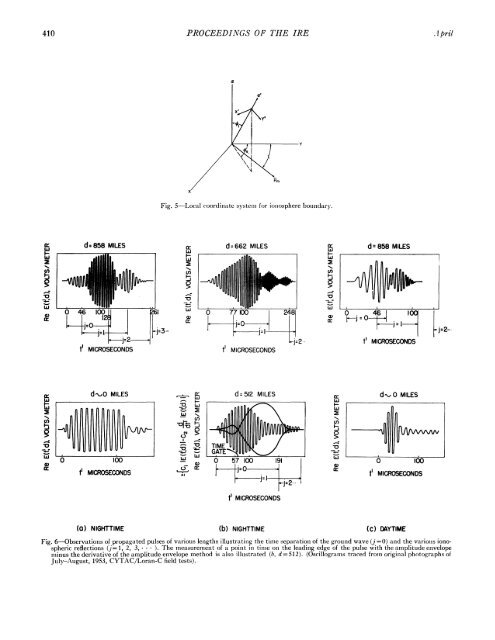
1962 Johler: <strong>Propagation</strong> of <strong>Low</strong>-<strong>Frequency</strong> Signal 409 $_ - Ray Indicating Electric Vector in Plane of Vertical Electric Sourte and Observor Dipoles --- Ray Indicating Magnetic Vector in Some Plane Hm Ns V 0 I- Hm,tl,N,9 V HM,2, N2t V2 E 0 W 0 ,P 0 E 0 v - R - -r- cr, E2 Hm,1, Ni,1Vi Hm,21 N2' V2 HM,3, N3 Z3 ,n,~~ ~ / 0*, E Ev EE 0 we EEE ow E Es 1')~~ N ~~~~~ / \\ // E cc r crI,' 2,1 )^^^^^ E 0 E 0 cr sl: tz: {k (2, l2,2 Hm,l Nj, 1/1 HM,21 N2, 1/2 Hm,3, N31 V3 Hm 49 N4, £V E E E 0 E E 0 E @ 0 w @ 0 0 we E E _|_E E we E EFwe EFvE;E L-.;- _ _ M CY to to n o g E vE EEwEOEEw c: cr a:. cr ta:Cr_ :z c. :. cr.r :zrc 0-i , I2, 07. (62,2 O3. - 62,3 Fig. 4-Geometric-optical ray propagation mechanism, illustrating the development of the factor C3 and illustrating coupling exterior to the ionosphere as a consequence of the generation of the abnormal components. plane wave and a similar vertical electric polarization of the reflected wave. The coefficient Ter describes the generation of the abnormal component by the incident vertical polarization (reflected horizontal electric polarization for vertical electric excitation). Similarly, Trm refers to the incident horizontal electric polarization and the corresponding reflected horizontal electric polarization. Also, the abnormal component of the horizontal electric polarization (reflected vertical electric polarization for horizontal electric excitation) is described by the coefficient Tine. Referring these matters to a local coordinate system (Fig. 5) at the ionosphere lower boundary [12], [19], [20], Tee = Ey'r/Ey'is Tem = Ex'r/Ey'i Trmn-= Ex'r/Ex,ij Tmie = EyrlExt (37) where the subscripts i or r refer to the incident and reflected wave, respectively, at the lower boundary of the ionosphere. The techniques for evaluating the reflection coefficients for an anisotropic model electron-ion plasma are quite complicated and will be discussed later. The ground wave CW, Eo(w, d) (i.e., the zero order ray j=0 can be evaluated from the classical series of residues) formulated by Bremmer can be written in the form [1], [13 ], [23 ] for vertical electric polarization = 2icoC [27ra2/3(kia)113 +11/2 E(w, d) =2icoC 2eraXl 3(kia) 113 - f ~ ~ ~d aed r~ exp {i (kia)1/3ra2/3 -+ _- + -_] s=0 [2r-11,/6] _- (38) where s=0, 1, 2, 3, * * *, C is given by (9), and again a-0.75 to 0.85 and 6, Sr have been defined (32), (33). A horizontally-polarized Hertz dipole radiation field can also be found (vertical magnetic field, HI, ampereturns/meters) simply by replacing be by 6l. &.. = 6,ki/k2 re-evaluating ,r and substituting in (38). The notion of a CW signal E(o, d) as the vector sunm of individual rays ordered in timne (7) is obscure to the observer of such a signal. However, a signal in the true sense, i.e., oIne which can convey informationi and henice is interrupted in the time domain, manifests the individual propagation rays. The Fourier integral (1) for a pulse transmission can be rewritteni as a consequence of propagation of such signials E(t, d), p E(t', d) = > Ej(t'1, d) j=o P 1 C0X = exp (iwt'j)Ej(w, d)fr((w)f8(&)dw. (39) j7o 27r _ This merely represents the sum of separate Fourier integrals for each ray, separated in time by the ionospheric wave delay t'j. The signal E(t', d), (1), (39) which has been described in the time domain, is in general complex if complex source functions Fj(t), (3) are employed. The signal
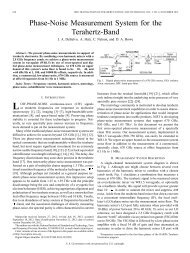
410 PROCEEDINGS OF THE IRE A pril w w N. a1) N -C Li} : a. d 858 MILES t' MICROSECONDS d_o MILES I MICROSECONDS Fig. 5-Local coordinate system for ioniosphere botundary. LLw I- w N C,) -J 0> -o w 0L) r - ,o W N U) -,. i0 h -1w waL) +1 d-662 MILES cr. d=d858 MILES w w tI MICROSECONDS N C,) w-r d = 512 MILES a: w w (I) t' MICROSECONDS (a) NIGHTTIME (b) NIGHTTIME 0 4 00 Q& 1M=ICRO ECN ~0 i:ri Q) cc tl MICOECODS d_-O MILES F 0 I 100 tI' MICROSECONDS Fig. 6-Observations of propagated pulses of various lengths illustrating the time separation of the grounid wave (j =0) and the various iono- spheric reflections (j= 1, 2, 3, * * - (C) DAYTIME W/v\/V The measurement of a point in tinme oni the leading edge of the pulse with the amplitude envelope ). minus the derivative of the amplitude envelope method is also illustrated July-August, 1953, CYTAC/Loran-C field tests). (b, d=512). (Oscillograms traced frorn original photographs of