Real-Time Control Lecture - MAELabs UCSD

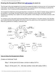
Requirements
Modeling
Open-Loop Survey
Proportional Control
PID Control
Robustness
Real-Time Control
MAE 156A

What does your system need to do?
Requirements
Feedback control can be expensive – are you sure that you need it?
Passive Control = no electronic components (e.g. water level)
Active Control = electronic components (e.g. cruise control)
reference
Control Actuator
Sensors
MAE 156A
noise
noise
Mechanical
System
2

Modeling
Developing an accurate system model is important because a small time investment
at the beginning of a project can save huge amounts of time later
Modeling is needed to verify design choices
Modeling is needed to select components
You might as well get organized and build a complete system model
Components or suppliers will change – and you don't want to repeat the entire design cycle
over again.
An accurate model can be used to develop test procedures and methods
Try a new idea on the model first (before you embarrass yourself in the lab)
MAE 156A
3

V c
(-)
1
L
R s1
Block Diagram : Motor and Table
K t
R
V_c = motor command voltage
L = armature inductance
R = armature resistance
K_t = torque constant
K_e = back EMF constant
T_m = motor torque
T m ˙
r t
r m
r t
r
m K e
MAE 156A
(-)
±D
1
Js
J = equivalent moment of inertia (at table)
D = equivalent friction (at table)
theta = table angular position
r_t = table radius
r_m = motor shaft radius
1
s
4

Open-Loop System Survey
An open-loop system survey is used to study the system dynamics.
Is the system dynamic model accurate enough?
What are system dynamic characteristics?
Determine open-loop system transfer functions
Identify nonlinear functions and behavior
Make following assumptions to find the open-loop transfer function of motor + table
Armature dynamics are “fast”: L/R is a small number
Dry friction acts like viscous friction
s
V c s =
r t /r m K t / R
J s 2 [ D' K t / Rr t / r m 2 K e ]s
MAE 156A
D '≈ D
∣ ˙ max∣
5

Motor Drive
Pot A/D Counts
300
200
100
0
-100
-200
Open-Loop Test Data
-300
0 0.1 0.2 0.3 0.4 0.5 0.6 0.7 0.8 0.9 1
600
500
400
300
200
100
0
0 0.1 0.2 0.3 0.4 0.5 0.6 0.7 0.8 0.9 1
MAE 156A
added weight
Time (sec)
Time (sec)
6

A set
(-)
Aset = pot count set point
A = pot count
Block Diagram : Closed-Loop
time
control
driver motor + table
delay
±255 board
K s e − d s
A
K(s) = control system dynamics
G(s) = motor + table dynamics
Q
MAE 156A
N
tau_d = time delay
V c
G s
N = motor driver board conversion [V/count]
Q = table position to pot [count/rad]
7

Proportional Control
Start with a simple control scheme that sets the motor drive voltage proportional to
the set point error.
K s=K p = proportional gain
Approximate time delay using a first-order lag filter.
e − d ≃ 1
d s1
The closed-loop characteristic equation is:
J d s 3 D' ' d J s 2 D' ' sK p QN r t /r m K t / R=0
D ' ' =D ' K t / Rr t /r m 2 K e
MAE 156A
8

K s=K p
Root Locus for Varied Kp
K p ∞
0
-120 -100 -80 -60 -40 -20 0 20
MAE 156A
Imaginary
60
40
20
-20
-40
-60
K p ∞
K p ∞
Real
Open-Loop Pole
9

Motor Drive
Pot A/D Counts
300
200
100
0
-100
-200
Proportional Control
-300
0 0.2 0.4 0.6 0.8 1 1.2 1.4 1.6 1.8 2
1000
800
600
400
200
0
0 0.2 0.4 0.6 0.8 1 1.2 1.4 1.6 1.8 2
MAE 156A
Time (sec)
Time (sec)
10

Pot A/D Counts Motor Drive
300
200
100
0
-100
-200
Limit Cycle Response
-300
0 0.2 0.4 0.6 0.8 1 1.2 1.4 1.6 1.8 2
1000
800
600
400
200
0
0 0.2 0.4 0.6 0.8 1 1.2 1.4 1.6 1.8 2
MAE 156A
Time (sec)
Time (sec)
11

K s=K p K d s
K d
K p
=1
Root Locus for PD Control
K p ∞
0
-60 -50 -40 -30 -20 -10 0 Real
K p ∞
MAE 156A
Imaginary
150
100
50
-50
-100
-150
Open-Loop Pole
12

Pot A/D Counts Motor Drive
300
200
100
0
-100
-200
Proportional + Derivative Control
-300
0 0.2 0.4 0.6 0.8 1 1.2 1.4 1.6 1.8 2
1000
800
600
400
200
0
0 0.2 0.4 0.6 0.8 1 1.2 1.4 1.6 1.8 2
MAE 156A
Time (sec)
Time (sec)
13

Implementation Issues
Numerical differentiation tends to amplify noise
Consider adding a lag filter to smooth the response
K s=K p K i
s K d s≃K p K i
s K d s
q s1
Numerical integration may lead to actuator drive saturation
Consider “anti-windup” integrator
is= K i
s [ A set s−As]
If amplitude of i(s) exceeds a
threshold, either reset i(s) = 0 or hold
i(s) at the threshold value.
MAE 156A
q = smoothing time constant
14

Loop Time Considerations
Numerical integration and differentiation depend upon loop time step.
What happens if you change the loop time step?
Laplace Domain
Time Domain
Discrete Time
d s=K d s [ A set s−As] =K d
d t=K d ˙et
d [k ]≃K d
d [k ]≃ K d
e [k ]−e[k −1]
e[k ]−e[k −1]
MAE 156A
s es
k =loop counter
=time step
A change in the loop
time step alters the
effective derivative gain!
15

Robustness
A closed-loop system exhibits robustness if its response characteristics are
insensitive to parameter variations and noise.
Parameter variations are likely to occur through normal wear
Expected wear should be considered as part of the overall life cycle design
Noise may depend on environment and operating conditions
Gain and phase margins are traditional measures of robustness
Gain margin measures tolerance to loop gain variations
Phase margin indicates tolerance to loop phase variations
Phase margin also measures tolerance to loop time delay
Other robustness tests are possible using a model simulation
Consider random variations in each model parameter
Robustness results become part of your system's performance specification
MAE 156A
16

Summary
Even a low-fidelity model can help you understand the underlying dynamics.
Don't be afraid of nonlinear elements – there is often an approximation available.
Keep track of loop step time as your design progresses.
Your effective control gains may change with time step
Large time delays reduce phase margin
Debugging real-time control firmware can be frustrating if you don't carefully consider
each code modification.
When in doubt, print out intermediate results!
MAE 156A
17