Lecture 2 - Internet Analysis Seminar
Lecture 2 - Internet Analysis Seminar
Lecture 2 - Internet Analysis Seminar
You also want an ePaper? Increase the reach of your titles
YUMPU automatically turns print PDFs into web optimized ePapers that Google loves.
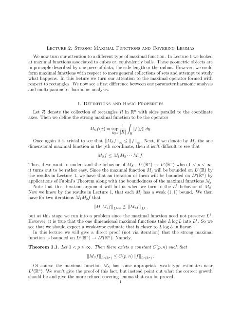
<strong>Lecture</strong> 2: Strong Maximal Functions and Covering Lemmas<br />
We now turn our attention to a different type of maximal function. In <strong>Lecture</strong> 1 we looked<br />
at maximal functions associated to cubes or, equivalently balls. These geometric objects are<br />
in principle described by one piece of data, the side length or the radius. However, we could<br />
form maximal functions with respect to more general collections of sets and attempt to study<br />
what happens. In this lecture we turn our attention to the maximal operator formed with<br />
respect to rectangles. We now see a first difference between one parameter harmonic analysis<br />
and multi-parameter harmonic analysis.<br />
1. Definitions and Basic Properties<br />
Let R denote the collection of rectangles R in Rn with sides parallel to the coordinate<br />
axes. Then we define the strong maximal function to be the operator<br />
<br />
1<br />
MSf(x) = sup |f(y)| dy.<br />
R∋x |R|<br />
Once again it is trivial to see that MSf ∞ ≤ f ∞ . Next, if we denote by Mj the one<br />
dimensional maximal function in the jth coordinate, then it isn’t difficult to see that<br />
R<br />
MSf ≤ M1M2 · · · Mnf.<br />
Thus, if we want to understand the behavior of MS : L p (R n ) → L p (R n ) when 1 < p < ∞,<br />
it turns out to be rather easy. Since the maximal function Mj will be bounded on L p (R) by<br />
the results in <strong>Lecture</strong> 1, we have that an iteration of them will be bounded on L p (R n ) by<br />
applications of Fubini’s Theorem along with the boundedness of the maximal functions Mj.<br />
Note that this iteration argument will fail us when we turn to the L 1 behavior of MS.<br />
Now we know by the results in <strong>Lecture</strong> 1, that each Mj has a weak (1, 1) bound. We then<br />
have for two iterations M1M2f that<br />
M1M2f L 1,∞ M2f L 1 ,<br />
but at this stage we run into a problem since the maximal function need not preserve L 1 .<br />
However, it is true that the one dimensional maximal functions take L log L into L 1 . So we<br />
see that we should expect a weak-type estimate that is closer to L log L in flavor.<br />
In this lecture we will give a direct proof (not via iteration) that the strong maximal<br />
function is bounded on L p (R n ) → L p (R n ). Namely,<br />
Theorem 1.1. Let 1 < p ≤ ∞. Then there exists a constant C(p, n) such that<br />
MSf L p (R n ) ≤ C(p, n) f L p (R n ) .<br />
Of course the maximal function MS has some appropriate weak-type estimates near<br />
L 1 (R n ). We won’t give the proof of this fact, but instead point out what the correct growth<br />
should be and give the more refined covering lemma that can be proved.<br />
1
2<br />
2. Estimates for the Strong Maximal Function<br />
In this section we turn to understanding the proof of the covering lemma that will be<br />
useful to prove the L p boundedness of the strong maximal function. We will accomplish this<br />
by proving a covering lemma and then proving that covering lemmas are in fact equivalent<br />
to estimates for the maximal function.<br />
Theorem 2.1 (A Covering Lemma for the Strong Maximal Theorem). Suppose that {Rj}j∈J<br />
is a family of rectangles in Rn with sides parallel to the axes. Then there is a sequence of<br />
rectangles { ˜ Rk} ⊂ {Rj}j∈J that satisfy<br />
<br />
<br />
(a) <br />
j∈J Rj<br />
<br />
<br />
≤ c(n) <br />
k ˜ <br />
<br />
Rk<br />
(b) <br />
p <br />
≤ C(n) <br />
<br />
<br />
k χ ˜ Rk<br />
L p (R n )<br />
j∈J Rj<br />
The main point behind (a) is that it is possible to select a sub-collection of the given<br />
rectangles so that the size of the collected set is still comparable to the original collection.<br />
Proof. The proof is by induction on the dimension. Suppose that the Theorem is true for<br />
n−1, then we will show how to get the Lemma in the case of n. Note that since the Theorem<br />
is true for n − 1 by Theorem 1.1 we have that the maximal operator M n−1<br />
S : Lp (Rn−1 ) →<br />
Lp (Rn−1 ) is bounded when 1 < p < ∞.<br />
For a rectangle S ⊂ Rn , let ˆ S denote the rectangle obtained by keeping all the sides of S<br />
the same except the nth side, which we triple in size. Given the collection {Rj}, first relabel<br />
if necessary so that the Rj are ordered so that their nth sidelengths decrease. We now give<br />
a selection procedure to find the desired collection of rectangles. Take ˜ R1 = R1 and let ˜ R2<br />
be the first rectangle Rk such that<br />
<br />
<br />
Rk ∩ ˜ <br />
<br />
R1<br />
< 1<br />
2 |Rk| .<br />
Suppose have now chosen the rectangles ˜ R1, ˜ R2, . . . , ˜ Rj−1. We select ˜ rectangle occurring after<br />
Rj to be the first<br />
˜ Rj−1 so that<br />
<br />
<br />
<br />
<br />
Rk<br />
<br />
<br />
˜ˆRl ∩ < 1<br />
2 |Rk| .<br />
l
inequality note that if Ri is not a selected rectangle, the we must have<br />
<br />
<br />
<br />
<br />
Ri<br />
<br />
n−1<br />
˜ˆRj ∩<br />
≥ 1<br />
2 |Ri| = 1<br />
2 |Ti| n−1 |Ii| .<br />
j<br />
Note that we haven’t used the condition on the decreasing side lengths yet. Here we now<br />
exploit this fact to conclude that<br />
<br />
<br />
<br />
<br />
Ti<br />
<br />
n−1<br />
˜ˆTj ∩<br />
≥ 1<br />
2 |Ti| n−1 .<br />
Now note that (2.1) implies that<br />
(2.2) M n−1<br />
S<br />
and so we have for all points x ∈ ∪Ti that<br />
<br />
<br />
ˆTi ⊂<br />
j<br />
<br />
M n−1<br />
S<br />
χS ˜ ˆTj<br />
<br />
<br />
(x) ≥ 1<br />
2<br />
χS ˜ ˆTj<br />
<br />
(x) ≥ 1<br />
<br />
.<br />
2<br />
Since for points in selected rectangles, this containment is obvious, while for points in the<br />
non-selected rectangles, (2.2) gives the containment. This then implies<br />
<br />
<br />
<br />
<br />
Ti<br />
n−1<br />
≤<br />
<br />
<br />
<br />
M n−1<br />
<br />
S χS <br />
Tj<br />
˜ (x) ≥ 1<br />
<br />
<br />
2<br />
<br />
≤ C<br />
Rn−1 =<br />
χS ˜ (x)dx ˆTj<br />
<br />
<br />
C <br />
˜ˆTj <br />
.<br />
n−1<br />
Here we have used the induction hypothesis that M n−1<br />
S<br />
: L p (R n−1 ) → L p (R n−1 ) is bounded<br />
when 1 < p < ∞ coupled with Chebyshev’s Inequality for p. Finally, integrate this inequality<br />
over the nth coordinate to arrive at<br />
<br />
<br />
<br />
≤ C ˜Rj <br />
<br />
Ri<br />
which proves (i) in the Covering Lemma.<br />
Now, we turn to (ii). We want to show that the function χ S ˜ R belongs to L p (R n ). To<br />
accomplish this, we will use a duality argument and test it against f ∈ Lp′ (Rn ) and show<br />
we have good estimates.<br />
With this in mind, note that if we define the sets<br />
˜Ej = ˜ Tj<br />
ˆ \ <br />
˜ˆTl<br />
then (2.1) gives that<br />
l 1<br />
<br />
<br />
<br />
2<br />
ˆ <br />
<br />
Tj<br />
n−1<br />
.<br />
3
4<br />
Choose f ∈ Lp′ (Rn−1 ) of norm at most 1 (here we identify Rn−1 with the first n − 1<br />
coordinates). Then we have<br />
<br />
<br />
<br />
<br />
χTj ˜ (x)f(x)dx =<br />
R n−1<br />
R n−1<br />
j<br />
j<br />
j<br />
˜Tj<br />
f(x)dx<br />
= <br />
<br />
<br />
<br />
j<br />
˜ <br />
<br />
Tj<br />
<br />
<br />
˜ <br />
<br />
<br />
f(x)dx<br />
˜Tj Tj<br />
≤ 2 <br />
|Ej|<br />
j<br />
1<br />
<br />
<br />
˜ <br />
<br />
<br />
f(x)dx<br />
˜Tj Tj<br />
≤ 2 <br />
j<br />
|Ej| M n−1<br />
S f(x).<br />
The last inequality holds for any x ∈ ˜ Tj. ˆ This last sum can be recovered as in integral over<br />
the desired sets. In particular, we end up with<br />
<br />
<br />
<br />
χ ˜ (x)f(x)dx M ˆTj<br />
n−1<br />
S f(x)dx<br />
By duality, this last inequality gives that<br />
<br />
<br />
<br />
<br />
<br />
χ ˜ˆTj <br />
<br />
j<br />
S ˜ˆTk k<br />
≤ M n−1<br />
S<br />
≤ f L p ′ (R n−1 )<br />
≤<br />
L p (R n−1 )<br />
<br />
<br />
<br />
˜ˆTk <br />
<br />
<br />
<br />
<br />
˜ˆTk <br />
<br />
<br />
<br />
1<br />
˜ˆTk p<br />
<br />
f L p ′ (R n−1 )<br />
1<br />
p<br />
.<br />
<br />
<br />
<br />
˜ˆTk <br />
<br />
Now raise this inequality to the p power and integrate over the remaining coordinate to<br />
arrive at the statement in (ii). <br />
A collection of rectangles has the covering property Vq, 1 ≤ q ≤ ∞ if there exists constants<br />
C1 < ∞ and C2 > 0 so that given any family {Rj}J we can find a sequence { ˜ Rk} ⊂ {Rj}J<br />
such that <br />
<br />
(a) <br />
j∈J Rj<br />
<br />
<br />
≤ C2(n) <br />
k ˜ <br />
<br />
Rk<br />
(b) <br />
q <br />
≤ C1(n) <br />
<br />
.<br />
k χ ˜ Rk<br />
L q (R n )<br />
j∈J Rj<br />
Theorem 2.2 (Cordoba-Fefferman, [3]). The maximal operator MS is of weak-type (p, p) if<br />
and only if the collection of rectangles has the covering property Vq where 1 1 + = 1 and<br />
p q<br />
1 < p ≤ ∞.<br />
It is easy to see how Theorem 2.2 and Theorem 2.1 can be used to prove Theorem 1.1.<br />
Exercise 2.3. Prove Theorem 1.1 by applying Theorem 2.2 and Theorem 2.1.<br />
1<br />
p<br />
.<br />
1<br />
p
Proof of Theorem 2.2. One direction is immediate. Suppose the collection of rectangles has<br />
the covering property Vq. Fix λ > 0 and consider the set<br />
Then we have that Eλ = <br />
Eλ = {x ∈ R n : MSf(x) > λ}.<br />
j Rj where for each rectangle Rj we have<br />
λ < 1<br />
|Rj|<br />
<br />
Rj<br />
|f(y)| dy.<br />
Now apply the definition of Vq property to select a subcollection ˜ Rk. Then we have<br />
<br />
<br />
<br />
<br />
<br />
|Eλ| = Rj<br />
<br />
j<br />
<br />
<br />
<br />
<br />
≤ C2 ˜Rk<br />
<br />
<br />
<br />
k<br />
≤ C2<br />
<br />
<br />
|f(y)| dy<br />
λ ˜Rk k<br />
= C2<br />
<br />
λ Rn <br />
χ ˜ (y) |f(y)| dy<br />
Rk<br />
k<br />
≤ C2<br />
<br />
<br />
<br />
<br />
<br />
χRk ˜ fLp (Rn )<br />
λ <br />
This then gives that<br />
≤ C1C2<br />
λ<br />
= C1C2<br />
λ<br />
k<br />
<br />
<br />
<br />
<br />
<br />
j<br />
Rj<br />
L q (R n )<br />
<br />
<br />
<br />
<br />
<br />
1<br />
q<br />
fLp (Rn )<br />
|Eλ| 1<br />
q f L p (R n ) .<br />
|Eλ| ≤ C<br />
fp<br />
λp Lp (Rn )<br />
which is the desired weak-type estimate.<br />
For the converse, suppose that MS satisfies the weak-type estimates. Given a family of<br />
rectangles {Rj}, we assume the existence of a subsequence { ˜ Rk} such that<br />
<br />
<br />
<br />
<br />
<br />
<br />
RJ<br />
≤ C ˜Rk<br />
<br />
<br />
<br />
and with the following disjointness property:<br />
<br />
<br />
<br />
<br />
˜ Rk ∩ <br />
<br />
<br />
˜Rj<br />
1<br />
<br />
<br />
≤ <br />
2<br />
˜ <br />
<br />
Rk<br />
∀k.<br />
j<br />
j
6<br />
Based on these sets, define Ek = ˜ Rk \ <br />
j
Theorem 3.1 (Cordoba, Fefferman). Suppose that {Rj}j∈J is a family of rectangles in Rn with sides parallel to the axes. Then there is a sequence of rectangles { ˜ Rk} ⊂ {Rj}j∈J that<br />
satisfy<br />
<br />
<br />
(a) <br />
j∈J Rj<br />
<br />
<br />
≤ c(n) <br />
k ˜ <br />
<br />
Rk<br />
<br />
<br />
(b) exp <br />
<br />
1<br />
n−1 <br />
<br />
≤ C(n) <br />
<br />
<br />
k χ ˜ Rk<br />
L 1 (R n )<br />
j∈J Rj<br />
If one uses this covering Lemma in conjunction with the methods of this <strong>Lecture</strong> we arrive<br />
at the weak-type estimates associated to the strong maximal function.<br />
Theorem 3.2. The operator MS is bounded from the Orlicz space L(log L) n−1 (Rn ) to L1,∞ (Rn ).<br />
Namely, for any f ∈ L(log L) n−1 and any λ > 0<br />
|{x ∈ R n : Msf(x) > λ}| ≤ C<br />
<br />
|f(x)| 1 + log<br />
λ<br />
|f(x)|<br />
<br />
n−1<br />
dx<br />
λ<br />
Exercise 3.3. Carry out the details to arrive at the above Theorem.<br />
R n<br />
References<br />
[1] A. Córdoba and R. Fefferman, On differentiation of integrals, Proc. Nat. Acad. Sci. U.S.A. 74 (1977),<br />
no. 6, 2211–2213. ↑<br />
[2] A. Cordoba and R. Fefferman, A geometric proof of the strong maximal theorem, Ann. of Math. (2) 102<br />
(1975), no. 1, 95–100. ↑<br />
[3] A. Córdoba and R. Fefferman, A geometric proof of the strong maximal theorem, Bull. Amer. Math. Soc.<br />
81 (1975), no. 5, 941. ↑4<br />
[4] Norberto Angel Fava, Weak type inequalities for product operators, Studia Math. 42 (1972), 271–288. ↑<br />
[5] R. Fefferman, Strong differentiation with respect to measures, Amer. J. Math. 103 (1981), no. 1, 33–40.<br />
↑<br />
[6] Robert Fefferman and Jill Pipher, A covering lemma for rectangles in R n , Proc. Amer. Math. Soc. 133<br />
(2005), no. 11, 3235–3241 (electronic). ↑<br />
7


