1. Introduction 2. Flow models of exchange rate determination
1. Introduction 2. Flow models of exchange rate determination
1. Introduction 2. Flow models of exchange rate determination

Create successful ePaper yourself
Turn your PDF publications into a flip-book with our unique Google optimized e-Paper software.
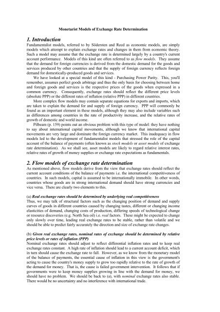
Monetarist Models <strong>of</strong> Exchange Rate Determination<br />
<strong>1.</strong> <strong>Introduction</strong><br />
Fundamentalist <strong>models</strong>, referred to by Södersten and Reed as economic <strong>models</strong>, are simply<br />
<strong>models</strong> which attempt to explain <strong>exchange</strong> <strong>rate</strong>s and changes in them from economic theory.<br />
Such a model may assume that the <strong>exchange</strong> <strong>rate</strong> is determined largely by a country's current<br />
account performance. Models <strong>of</strong> this kind are <strong>of</strong>ten referred to as flow <strong>models</strong>. They assume<br />
that the demand for foreign currencies is derived from the domestic demand for the goods and<br />
services produced by other countries and that the supply <strong>of</strong> foreign currency reflects foreign<br />
demand for domestically-produced goods and services.<br />
We have looked at a special model <strong>of</strong> this kind - Purchasing Power Parity. This, you'll<br />
remember, assumes perfect goods arbitrage and thus the only basis for choosing between home<br />
and foreign goods and services is the respective prices <strong>of</strong> the goods when expressed in a<br />
common currency. Consequently, <strong>exchange</strong> <strong>rate</strong>s should reflect the different price levels<br />
(absolute PPP) or the different <strong>rate</strong>s <strong>of</strong> inflation (relative PPP) in different countries.<br />
More complex flow <strong>models</strong> may contain sepa<strong>rate</strong> equations for exports and imports, which<br />
are taken to explain the demand for and supply <strong>of</strong> foreign currency. PPP will commonly be<br />
found as an important element in these <strong>models</strong>, although they may also include variables such<br />
as differences among countries in the <strong>rate</strong> <strong>of</strong> productivity increase, and the relative <strong>rate</strong>s <strong>of</strong><br />
growth <strong>of</strong> domestic and world income.<br />
Pilbeam (p. 159) points out an obvious problem with this type <strong>of</strong> model: they have nothing<br />
to say about international capital movements, although we know that international capital<br />
movements are very large and dominate the foreign currency market. This inadequacy in flow<br />
<strong>models</strong> led to the development <strong>of</strong> fundamentalist <strong>models</strong> that stressed the role <strong>of</strong> the capital<br />
account <strong>of</strong> the balance <strong>of</strong> payments (<strong>of</strong>ten known as stock <strong>models</strong> or asset <strong>models</strong> <strong>of</strong> <strong>exchange</strong><br />
<strong>rate</strong> <strong>determination</strong>). As we shall see, asset <strong>models</strong> are likely to regard relative interest <strong>rate</strong>s,<br />
relative <strong>rate</strong>s <strong>of</strong> growth <strong>of</strong> money supplies or <strong>exchange</strong> <strong>rate</strong> expectations as fundamentals.<br />
<strong>2.</strong> <strong>Flow</strong> <strong>models</strong> <strong>of</strong> <strong>exchange</strong> <strong>rate</strong> <strong>determination</strong><br />
As mentioned above, flow <strong>models</strong> derive from the view that <strong>exchange</strong> <strong>rate</strong>s should reflect the<br />
current account conditions <strong>of</strong> the balance <strong>of</strong> payments i.e. the international competitiveness <strong>of</strong><br />
countries. In such <strong>models</strong>, capital is assumed to be internationally immobile. In other words,<br />
countries whose goods are in strong international demand should have strong currencies and<br />
vice versa. There are clearly two elements to this.<br />
(a) Real <strong>exchange</strong> <strong>rate</strong>s should be determined by underlying real competitiveness<br />
Thus, we may talk <strong>of</strong> structural factors such as the changing position <strong>of</strong> demand and supply<br />
curves <strong>of</strong> goods in different countries caused by changing tastes, different or changing income<br />
elasticities <strong>of</strong> demand, changing costs <strong>of</strong> production, differing speeds <strong>of</strong> technological change<br />
or resource discoveries (e.g. North Sea oil) i.e. real factors. These might be expected to change<br />
only slowly over time, leading real <strong>exchange</strong> <strong>rate</strong>s to be stable, rather than volatile and we<br />
should be able to predict fairly accu<strong>rate</strong>ly the direction and size <strong>of</strong> <strong>exchange</strong> <strong>rate</strong> changes.<br />
(b) Given real <strong>exchange</strong> <strong>rate</strong>s, nominal <strong>rate</strong>s <strong>of</strong> <strong>exchange</strong> should be determined by relative<br />
price levels or <strong>rate</strong>s <strong>of</strong> inflation (PPP)<br />
Nominal <strong>exchange</strong> <strong>rate</strong>s should adjust to reflect differential inflation <strong>rate</strong>s and to keep real<br />
<strong>exchange</strong> <strong>rate</strong>s constant. A high <strong>rate</strong> <strong>of</strong> inflation should lead to a current account deficit, which<br />
in turn should cause the <strong>exchange</strong> <strong>rate</strong> to fall. However, as we know from the monetary model<br />
<strong>of</strong> the balance <strong>of</strong> payments, the essential cause <strong>of</strong> inflation in this view is the government's<br />
acting to cause the country's money supply to grow too rapidly relative to the <strong>rate</strong> <strong>of</strong> growth <strong>of</strong><br />
the demand for money. That is, the cause is failed government intervention. It follows that if<br />
governments were to keep money supplies growing in line with the demand for money, we<br />
should have no problem. We should be back to (a), with nominal <strong>exchange</strong> <strong>rate</strong>s also stable.<br />
There would be no uncertainty and no interference with international trade.
The simplest model eliminates (b) above by assuming fixed prices. For such a model to<br />
produce a stable <strong>exchange</strong> <strong>rate</strong>, the Marshall-Lerner condition must be satisfied, so that a<br />
current balance deficit will be corrected by the consequent fall in the value <strong>of</strong> the domestic<br />
currency. However, as we have seen, the Marshall-Lerner condition is unlikely to be satisfied<br />
in the short run - a depreciation <strong>of</strong> a currency is likely to make the current account worse before<br />
it gets better (the J-curve).<br />
<strong>2.</strong>1 <strong>Flow</strong> Models and the J-Curve<br />
The J-curve arises because the effect <strong>of</strong> a change in <strong>exchange</strong> <strong>rate</strong> on the current account<br />
consists <strong>of</strong> two elements:<br />
(i) the relative prices <strong>of</strong> home and foreign goods are altered - the fall in the <strong>exchange</strong> <strong>rate</strong> means<br />
that firms now pay more for imports in terms <strong>of</strong> domestic currency than previously (or receive<br />
less foreign currency for exports); and<br />
(ii) the relative price changes lead to quantity changes i.e. an increased foreign demand for<br />
exports and a reduced home demand for imports.<br />
(i) by itself plainly makes the current account worse. It is only when quantity effects begin<br />
to appear that (assuming favourable elasticities) the current account may begin to improve. The<br />
problem is that the impact <strong>of</strong> (i) is immediate, while quantity changes may take 18 months or<br />
longer to occur. This is due to lack <strong>of</strong> information, consumer inertia and the fact that some<br />
consumers will be locked into contracts that prevent them switching rapidly from one source <strong>of</strong><br />
supply to another.<br />
Let us translate this into the foreign <strong>exchange</strong> market. Assume that we begin with current<br />
account balance but that then there is a fall in demand for the home country's exports. This<br />
leads to a fall in demand for the home currency (a fall in the supply <strong>of</strong> foreign currency). In<br />
Fig. 1, the supply <strong>of</strong> foreign currency shifts up from S1 to S<strong>2.</strong> The new equilibrium <strong>exchange</strong><br />
<strong>rate</strong> will be at B (the value <strong>of</strong> the home currency has fallen sufficiently to bring the current<br />
account <strong>of</strong> the balance <strong>of</strong> payments back into equilibrium). In practice, however, the price<br />
effect occurs on its own: the fall in the value <strong>of</strong> the home currency requires foreigners to pay<br />
less foreign currency for the same quantity <strong>of</strong> imports as before. The supply <strong>of</strong> foreign<br />
currency falls further than is needed to restore current account balance (the supply curve shifts<br />
to S3, producing a temporary <strong>exchange</strong> <strong>rate</strong> <strong>of</strong> C. As soon as the quantity effects begin to<br />
appear, there will be pressures in the opposite direction. However, this could take a<br />
considerable time to occur and the <strong>exchange</strong> <strong>rate</strong> could, in the short run, overshoot its long-run<br />
equilibrium position by a long way.<br />
Exchange<br />
Rate (units <strong>of</strong> S3 S2 S1<br />
home currency C<br />
per unit <strong>of</strong> B<br />
foreign currency) A<br />
O<br />
Fig. 1<br />
foreign currency<br />
It is also possible that once the quantity effects begin to dominate and the <strong>exchange</strong> <strong>rate</strong><br />
falls again from C, it will move beyond B. The <strong>exchange</strong> <strong>rate</strong> should, within an overall stable<br />
model, eventually settle at B, but there might be considerable volatility around that <strong>rate</strong>.<br />
Further, before we settle at B, there may have been other long-term changes which cause B to
e no longer the long-term equilibrium <strong>exchange</strong> <strong>rate</strong> and the whole process will begin again.<br />
We might never, then, settle at a long-term equilibrium <strong>rate</strong>.<br />
This provides the simplest <strong>exchange</strong> <strong>rate</strong> overshooting model. Note that it is based upon<br />
two things occurring at different speeds: the price effect and the quantity effect. We shall return<br />
to this idea <strong>of</strong> different speeds <strong>of</strong> response later.<br />
<strong>2.</strong>2 Overcoming the J-Curve Problem<br />
The easiest way out <strong>of</strong> this dilemma is to introduce the capital account <strong>of</strong> the balance <strong>of</strong><br />
payments and allow for capital mobility, but to make particular assumptions regarding the<br />
capital market: that speculators within it are well-informed and act to smooth out excess<br />
demands and supplies <strong>of</strong> currencies, thus keeping <strong>exchange</strong> <strong>rate</strong>s stable.<br />
The central support for this assumption comes from the proposition that speculators are<br />
only operating in the market to make a pr<strong>of</strong>it and will only stay in the market if they are doing<br />
so. To make a pr<strong>of</strong>it, they must guess correctly the longer-term direction <strong>of</strong> the market so that<br />
they can buy cheap and sell dear. This will cut <strong>of</strong>f the lows and highs <strong>of</strong> <strong>exchange</strong> <strong>rate</strong><br />
fluctuations and ensure a stable market. Consider Fig. 1 once more. We again commence at A<br />
and again there is an autonomous fall in the demand for home goods.<br />
Speculators know (guess correctly) that the long-run equilibrium <strong>rate</strong> is B. Thus, as soon as<br />
the <strong>rate</strong> rises above B, they see that a pr<strong>of</strong>it is to be made from buying the home currency now<br />
and selling it later, once the <strong>exchange</strong> <strong>rate</strong> has again fallen. The very act <strong>of</strong> speculators in<br />
buying the home currency now will strengthen it in the market and prevent the <strong>exchange</strong> <strong>rate</strong><br />
from rising to C. Thus it is held that, in a free market, speculators will act to ensure the stability<br />
<strong>of</strong> <strong>exchange</strong> <strong>rate</strong>s.<br />
Naturally, there are several objections to this rosy picture. Firstly, there is the possibility <strong>of</strong><br />
capital movements from other sources - tourists, central banks, traders who take open positions<br />
in positions in foreign <strong>exchange</strong>. These may lose. Crucial to the argument is the nature <strong>of</strong><br />
expectations held within the market.<br />
If some people hold extrapolative expectations, then, as the value <strong>of</strong> the home currency<br />
falls, people will sell it and make things worse rather than better. However, this makes things<br />
better for the well-informed speculators who can still act to reduce market fluctuations.<br />
The second objection relates to the depth <strong>of</strong> the market. The optimistic view <strong>of</strong> speculation<br />
implies that the market is very deep and thus that individual speculators can have no impact on<br />
prices. It is this which requires them to act with the grain <strong>of</strong> the market in order to make a<br />
pr<strong>of</strong>it. Is this true?<br />
Suppose that there are some very large speculators operating within a thin market.<br />
Imagine, moreover, that other market participants hold extrapolative expectations. Now,<br />
imagine that, as the <strong>exchange</strong> <strong>rate</strong> begins to rise, the speculators move into the market in a big<br />
way, selling the home currency, forcing the <strong>exchange</strong> <strong>rate</strong> up still further. Other participants<br />
see the value <strong>of</strong> the home currency falling sharply and they too begin to sell. The <strong>exchange</strong> <strong>rate</strong><br />
rises even beyond C. Speculators then buy back in and take their pr<strong>of</strong>it. In this example,<br />
speculators destabilize the market, causing the <strong>exchange</strong> <strong>rate</strong> to fluctuate by more than it would<br />
otherwise have done.<br />
A different route <strong>of</strong> attack on stabilizing speculation is to reject the notion <strong>of</strong> speculators<br />
being well-informed and knowing the long-run equilibrium <strong>rate</strong>. Again, once capital<br />
movements are allowed into the model, we can have autonomous capital movements and the<br />
medium-term equilibrium in which the deficit on current account <strong>of</strong> the balance <strong>of</strong> payments is<br />
matched by a surplus on capital account (or vice-versa) will not necessarily be determined by<br />
current account changes. This makes it much more difficult for operators to know the longterm<br />
equilibrium <strong>rate</strong>.<br />
The notion <strong>of</strong> different levels <strong>of</strong> equilibrium over different time periods has been<br />
formalized in the classification <strong>of</strong> <strong>exchange</strong> <strong>rate</strong> theories in terms <strong>of</strong> four periods:<br />
A. very short period: <strong>exchange</strong> <strong>rate</strong>s mainly determined by capital flows;<br />
B. short period: overall equilibrium in the balance <strong>of</strong> payments but the capital account and the<br />
current account may both be out <strong>of</strong> balance;
C. long period: both capital account and current account in equilibrium;<br />
D. very long period: Purchasing Power Parity.<br />
3. Monetary Models <strong>of</strong> Exchange Rate Determination<br />
Models that concent<strong>rate</strong> on the capital account <strong>of</strong> the balance <strong>of</strong> payments are commonly<br />
known as stock <strong>models</strong>. These may, in turn, be divided into monetary <strong>models</strong> and asset (or<br />
portfolio) <strong>models</strong>. We look at monetary <strong>models</strong> here and consider asset <strong>models</strong> in the next<br />
section <strong>of</strong> the course.<br />
Monetary <strong>models</strong> develop from the Monetary Approach to the Balance <strong>of</strong> Payments<br />
(MAB). The <strong>exchange</strong> <strong>rate</strong> is seen as a relative asset price. The present value <strong>of</strong> an asset is<br />
thought to be largely influenced by its expected <strong>rate</strong> <strong>of</strong> return. As we have already seen, this<br />
provides the basis <strong>of</strong> uncovered interest <strong>rate</strong> parity (UIP). It would be useful at this point to<br />
compare Pilbeam's version <strong>of</strong> UIP with that presented to you earlier in the course (see notes on<br />
the forward <strong>exchange</strong> market).<br />
Pilbeam's definition (page 161) is that UIP holds when 'the expected <strong>rate</strong> <strong>of</strong> depreciation <strong>of</strong><br />
the pound-dollar <strong>exchange</strong> <strong>rate</strong> is equal to the interest <strong>rate</strong> differential between UK and US<br />
bonds'. Thus, if 'the expected <strong>rate</strong> <strong>of</strong> depreciation <strong>of</strong> the pound was 10 per cent, then according<br />
to UIP the UK <strong>rate</strong> <strong>of</strong> interest would have to be 10 per cent higher than the US interest <strong>rate</strong> to<br />
ensure the equalization <strong>of</strong> expected yields on UK and US bonds' (page 161). For further<br />
explanation see Box 7.1 and Figure 7.1 on page 163 <strong>of</strong> Pilbeam.<br />
You should note that for UIP to hold continuously, the following assumptions are required:<br />
• capital must be perfectly mobile;<br />
• investors must regard home and foreign bonds as equally risky (or must be risk neutral)<br />
In other words, domestic and foreign bonds must be perfect substitutes. Monetary <strong>models</strong> <strong>of</strong><br />
<strong>exchange</strong> <strong>rate</strong> <strong>determination</strong> make this assumption.<br />
Thus, we can say that in monetary <strong>models</strong>, economic agents are assumed to be indifferent<br />
as to the proportions <strong>of</strong> domestic and foreign assets - their only concern is that they yield the<br />
same return. The <strong>models</strong> assume (a) competitive markets; (b) negligible transactions costs; and<br />
(c) <strong>exchange</strong> <strong>rate</strong> expectations held with certainty (or risk-neutral investors). All <strong>models</strong> thus<br />
assume UIP. Further, they all assume that the key determinants <strong>of</strong> <strong>exchange</strong> <strong>rate</strong>s are the<br />
supply <strong>of</strong> and demand for money.<br />
Pilbeam deals with three monetary <strong>models</strong>: a flexible-price model, a sticky price model and<br />
a real interest-<strong>rate</strong> differential model.<br />
3.1 The Flexible-Price Monetary Model<br />
This model assumes that all prices in the economy are perfectly flexible, both upwards and<br />
downwards, even in the short run. Thus, PPP holds continuously and money markets clear<br />
continuously. There is a conventional demand for money function and thus,<br />
MSs = MDd = kpy ηηηη r -σσσσ<br />
....(1)<br />
That is, the demand for money is stably and positively related to real income (py) and<br />
negatively related to the <strong>rate</strong> <strong>of</strong> interest.<br />
or, as Pilbeam writes it,<br />
m - p = ηηηηy - σσσσr …. (2)<br />
where m is the log <strong>of</strong> the domestic money stock, p is the log <strong>of</strong> the domestic price level, y is the<br />
log <strong>of</strong> domestic real income and r is the <strong>rate</strong> <strong>of</strong> interest. The same relationship is assumed to<br />
hold abroad and thus:
m* - p* = ηηηηy* - σσσσr* …. (3)<br />
Since PPP is assumed to hold, we can write:<br />
s = p - p* ....(4)<br />
UIP holds continuously and thus,<br />
Es = r - r* ....(5)<br />
(the expected <strong>rate</strong> <strong>of</strong> depreciation <strong>of</strong> the home currency equals the difference between the<br />
domestic and foreign interest <strong>rate</strong>s).<br />
Re-arranging and substituting (see Pilbeam for details), gives:<br />
s = (m - m*) - ηηηη(y - y*) + σσσσ(r - r*) ....(6)<br />
That is, the <strong>rate</strong> <strong>of</strong> <strong>exchange</strong> is determined by the supply <strong>of</strong> money and the stock demand for<br />
money function at home and abroad. Ceteris paribus, the home currency appreciates (s falls):<br />
(a) if the domestic level <strong>of</strong> income rises relative to the foreign level <strong>of</strong> income;<br />
Thus, economic growth causes appreciation. This is seemingly in conflict with the standard<br />
Keynesian IS/LM/BP model in which an increase in domestic income causes imports to rise,<br />
worsening the balance <strong>of</strong> payments and producing a depreciation <strong>of</strong> the currency. In the<br />
monetary model, the money supply is assumed to be exogenous and thus an increase in<br />
domestic income causes the demand for money to increase. The only way in which money<br />
market equilibrium can be restored is through a fall in prices and, with PPP, the currency<br />
appreciates.<br />
(b) if interest <strong>rate</strong>s fall relative to foreign interest <strong>rate</strong>s;<br />
A fall in interest <strong>rate</strong>s leads to an increase in the demand for money and this (with the<br />
money stock given), requiring a fall in the transactions demand for money to maintain money<br />
market equilibrium. Again, with everything else assumed exogenous, this can only happen if<br />
prices fall and (with PPP) the currency appreciates. Pilbeam develops the reverse argument - an<br />
increase in the domestic interest <strong>rate</strong> causes the domestic currency to depreciate (s to rise). This<br />
also seems perverse until you look closely at the assumptions <strong>of</strong> the model. As well as using<br />
the argument I have employed here, Pilbeam (pages 166 and 167) by using the definition <strong>of</strong> the<br />
nominal interest <strong>rate</strong> as the real interest <strong>rate</strong> plus the <strong>rate</strong> <strong>of</strong> inflation and assuming (as we did in<br />
our discussion <strong>of</strong> the Fisher effect) that the real interest <strong>rate</strong> is constant and identical in all<br />
countries. It follows that an increase in domestic interest <strong>rate</strong>s implies an increase in<br />
inflationary expectations and this causes consumers to reduce their demand for money and<br />
increase their expenditure. Prices, then, do rise in line with expectations and the currency<br />
depreciates to maintain PPP. Hence, Pilbeam provides an alternative version <strong>of</strong> the monetary<br />
model equation (eqn. 7.9, p. 167) in which expected <strong>rate</strong>s <strong>of</strong> inflation replace interest <strong>rate</strong>s.<br />
(c) if the domestic money supply increases less rapidly than the foreign money supply.<br />
The underlying mechanism <strong>of</strong> the monetary model is that the <strong>exchange</strong> <strong>rate</strong> adjusts to<br />
maintain the law <strong>of</strong> one price in the presence <strong>of</strong> different domestic and world <strong>rate</strong>s <strong>of</strong> inflation<br />
(caused by different monetary growth <strong>rate</strong>s). As in the monetary balance <strong>of</strong> payments <strong>models</strong>,
the inflation <strong>rate</strong> and the <strong>exchange</strong> <strong>rate</strong> cannot be controlled simultaneously by the authorities if<br />
foreign prices are varying.<br />
The problem is that, as we have seen, there is evidence <strong>of</strong> substantial deviations from the<br />
law <strong>of</strong> one price since 1973. Consequently, it is hardly surprising (as Pilbeam notes) that the<br />
flexible price monetary model does not perform well in tests.<br />
3.2 Sticky-Price Monetarist Models<br />
We have already provided (through the J-curve) one possible reason for <strong>exchange</strong> <strong>rate</strong>s to<br />
overshoot long-run equilibrium <strong>rate</strong>s. Overshooting has been explained in several other <strong>models</strong><br />
which continue to assume the existence <strong>of</strong> long-run equilibrium <strong>rate</strong>s <strong>of</strong> <strong>exchange</strong> and<br />
incorpo<strong>rate</strong> both UIP and PPP. These <strong>models</strong> also typically assume rational expectations and<br />
so market participants are assumed to make the best available use <strong>of</strong> all relevant information<br />
and to employ the best available model for forecasting future <strong>exchange</strong> <strong>rate</strong>s. Therefore, they<br />
are assumed to know what the long-run equilibrium <strong>exchange</strong> <strong>rate</strong> is. Despite this, <strong>exchange</strong><br />
<strong>rate</strong>s are held to overshoot their long-run equilibrium positions. That is, when the <strong>exchange</strong> <strong>rate</strong><br />
is above its equilibrium it will fall well below the equilibrium <strong>rate</strong> before once again rising<br />
towards equilibrium. Equally, a rising <strong>exchange</strong> <strong>rate</strong> will rise above the equilibrium <strong>rate</strong> before<br />
falling towards it. This result is achieved by assuming that different elements in the model<br />
adjust at different speeds, as in the case <strong>of</strong> the J-curve. The best known such model was<br />
developed by the American economist, Dornbusch.<br />
3.<strong>2.</strong>1 Dornbusch's overshooting model<br />
In a well-known article in 1976, Dornbusch assumed all the usual conditions <strong>of</strong> a monetary<br />
model, including an exogenous money supply and, in the long run, PPP. Expectations are<br />
assumed to be regressive i.e. it is assumed that any movement away from equilibrium will<br />
immediately be reversed.<br />
Overshooting results in the model from the assumption that the goods and labour markets<br />
are slow to adjust (that is, prices in the goods market and wages in the labour market are sticky)<br />
whereas the asset market adjusts immediately. Exchange <strong>rate</strong>s are determined in the asset<br />
market and, thus, <strong>exchange</strong> <strong>rate</strong> changes are not matched, in the short run, by price changes.<br />
That is, we depart from PPP in the short run, although not (as noted above) in the long run.<br />
You should next read Pilbeam's simple explanation <strong>of</strong> the Dornbusch model (Section 7.7,<br />
pages 167-70). Next, we consider the model more formally.<br />
Formally, the <strong>exchange</strong> <strong>rate</strong> in the model is driven by:<br />
(a) uncovered interest parity (UIP)<br />
Es = r - r* ....(7)<br />
(b) the demand for real money balances being a stable function <strong>of</strong> real income and interest <strong>rate</strong><br />
m - p = ηηηηy - σσσσr …. (8)<br />
(c) the long-run <strong>exchange</strong> <strong>rate</strong> being determined by PPP:<br />
! = p - p* ....(9)<br />
but the short-run <strong>exchange</strong> <strong>rate</strong> being determined by<br />
(d) regressive <strong>exchange</strong> <strong>rate</strong> expectations:
Es = θθθθ(! - s) ....(10)<br />
where ! is the equilibrium or long-run <strong>exchange</strong> <strong>rate</strong> and θ > 0.<br />
That is, in each period the expected change in the <strong>exchange</strong> <strong>rate</strong> is given by a fraction (θ) <strong>of</strong><br />
the difference between its current value and the long-run equilibrium value.<br />
Thus, the model has four endogenous variables:<br />
• domestic interest <strong>rate</strong>;<br />
• the expected change in the <strong>exchange</strong> <strong>rate</strong>; and<br />
• the current value <strong>of</strong> the <strong>exchange</strong> <strong>rate</strong><br />
• the price level.<br />
.<br />
There are four exogenous variables:<br />
• the foreign interest <strong>rate</strong>;<br />
• the long-run equilibrium <strong>exchange</strong> <strong>rate</strong>;<br />
• real income; and<br />
• the stock <strong>of</strong> money.<br />
Substitution <strong>of</strong> equations gives:<br />
m - p = ηηηηy - σσσσr + ηηηησσσσ(! -s) ....(11)<br />
allowing us to solve for s.<br />
Alternatively, we could solve equation (8) for r; then solve (7) for Es and (10) for s.<br />
The diagrammatic solution <strong>of</strong> the model gives a relationship between the <strong>exchange</strong> <strong>rate</strong> and<br />
the price level with the asset market always in equilibrium as in Fig. 2, in which equilibrium is<br />
at N, with p e and s e . Note that the <strong>exchange</strong> <strong>rate</strong> is here expressed in direct terms. That is, as<br />
we move along the horizontal axis s increases but this means that the value <strong>of</strong> the home<br />
currency falls (one has to pay more home currency for one unit <strong>of</strong> foreign currency).<br />
Price<br />
Level A<br />
p e<br />
X<br />
N<br />
O s e<br />
Figure 2<br />
A<br />
PPP<br />
X<br />
S
In this diagram, AA represents asset market equilibrium. Why does it slope down to the<br />
right? There are 3 steps in the argument:<br />
<strong>1.</strong> If p is low, the real value <strong>of</strong> the exogenous money supply will be high; thus for equilibrium,<br />
the demand for money must also be high. However, if p is low and y is constant at its full<br />
employment level, the demand for money will only be high if the domestic interest <strong>rate</strong> is low.<br />
Thus, in equilibrium if p is low, r must also be low (p and r positively related).<br />
<strong>2.</strong> If r is low, then to satisfy UIP and persuade investors to hold domestic bonds, they must<br />
expect a future appreciation <strong>of</strong> the <strong>exchange</strong> <strong>rate</strong>. That is, given r*, if r is low, Es must be high<br />
and positive.<br />
3. But, with regressive expectations, people will expect an appreciation <strong>of</strong> the domestic<br />
currency (a fall in s) only if the value <strong>of</strong> the currency is now below its long-run equilibrium<br />
level (i.e. if s is above its long-run equilibrium level). Thus, if r is low, s must be high (r and s<br />
negatively related).<br />
Therefore, for asset market equilibrium, a low p will be associated with a relatively high s<br />
(and vice versa) (p and s negatively related). That is, if interest <strong>rate</strong>s on domestic bonds fall,<br />
currency will flow out to buy foreign currency bonds; if the <strong>exchange</strong> <strong>rate</strong> is fixed, this flow<br />
will continue until people come to expect a sufficient appreciation <strong>of</strong> the currency to balance<br />
the interest <strong>rate</strong> differential.<br />
XX represents equilibrium in the goods market. This slopes up because an increase in p<br />
will lead to a fall in domestic demand. There are two reasons for this:<br />
(i) an increase in p causes the real <strong>exchange</strong> <strong>rate</strong> to fall (competitiveness declines). To restore<br />
competitiveness, the value <strong>of</strong> the domestic currency must fall (s must rise). Thus, a high p is<br />
associated with a high s. If this were the only effect, the goods market would clear along a ray<br />
from the origin indicating PPP. But:<br />
(ii) an increase in p causes the real value <strong>of</strong> the exogenous money supply to fall. Domestic<br />
interest <strong>rate</strong>s will rise causing aggregate demand to fall. Thus, for the goods market to clear, s<br />
need not rise by as much as is suggested by the change in the real <strong>exchange</strong> <strong>rate</strong>. Hence, XX is<br />
flatter than the PPP line through the origin.<br />
Note that below XX there is excess demand for goods and prices will be rising. Above XX<br />
there is excess supply <strong>of</strong> goods and prices will be falling. We assume that the asset market is<br />
always in equilibrium (i.e. we are always on AA). Thus, if we are at M1, there will be an excess<br />
demand for goods and prices will rise slowly. We shall move along AA towards N (in fig. 2).<br />
As prices increase, aggregate demand falls and s falls (the domestic currency appreciates),<br />
compensating investors for low domestic interest <strong>rate</strong>s caused by the high real money balances.<br />
Assume now a once and for all increase in the supply <strong>of</strong> money. The AA curve shifts out<br />
to A 1 A 1 . There will be no permanent effect on the current account <strong>of</strong> the balance <strong>of</strong> payments<br />
and PPP will hold at the new equilibrium at N 1 (X 1 X 1 shifts up). Investors (holding rational<br />
expectations) realize this. The movement to long-run equilibrium takes place in two stages.<br />
We start at N. The unexpected increase in the money supply pushes up XX and the market<br />
knows that the new equilibrium will be at N 1 with an <strong>exchange</strong> <strong>rate</strong> <strong>of</strong> s e1 i.e. the market knows<br />
the domestic currency will depreciate.<br />
But because domestic prices are slow to rise, the initial effect is to increase real money<br />
balances and lower domestic interest <strong>rate</strong>s, causing people to sell domestic currency, pushing<br />
the <strong>exchange</strong> <strong>rate</strong> instantaneously to s<strong>2.</strong> At s2, investors can see the prospect <strong>of</strong> a sufficient<br />
<strong>exchange</strong> <strong>rate</strong> appreciation to compensate for the lower interest <strong>rate</strong> on domestic bonds and the<br />
currency depreciation ceases.
There follows a gradual adjustment to the new equilibrium <strong>exchange</strong> <strong>rate</strong>, s e1 , as prices<br />
increase in the goods market. Therefore, we have overshooting <strong>of</strong> the <strong>exchange</strong> <strong>rate</strong> even with<br />
rational expectations. If we dropped this assumption and assumed that the market did not know<br />
the long-run equilibrium position, they would try to infer the truth from what others were doing<br />
and there would be much wilder movements in s.<br />
Price<br />
Level A<br />
p e<br />
X<br />
N<br />
N 1<br />
O s e s e1 s 2<br />
Figure 3<br />
The Dornbusch model can be used to show that there will be no overshooting with fiscal<br />
policy. As is to be expected, the Dornbusch model does have its problems. These include:<br />
(a) It is very short run and doesn't allow for any adjustment to wealth.<br />
(b) The assumptions <strong>of</strong> infinite speed <strong>of</strong> adjustment <strong>of</strong> asset markets, risk-neutral investors and<br />
perfect substitutability <strong>of</strong> domestic and foreign bills are unrealistic.<br />
Many other similar <strong>models</strong> have been developed, distinguishing for example between the<br />
speeds <strong>of</strong> adjustment <strong>of</strong> the prices <strong>of</strong> tradeable and non-tradeable goods or <strong>of</strong> volumes and<br />
prices <strong>of</strong> exports and imports (known in the balance <strong>of</strong> payments literature as the J-curve). The<br />
central feature <strong>of</strong> all <strong>of</strong> these <strong>models</strong> is that they retain most <strong>of</strong> the assumptions <strong>of</strong> the standard<br />
economic approach to forex markets while attempting to produce results that are closer to the<br />
apparent reality <strong>of</strong> volatile <strong>exchange</strong> <strong>rate</strong>s. Thus, they can be grouped as part <strong>of</strong> the<br />
fundamentalist approach to forecasting <strong>exchange</strong> <strong>rate</strong>s.<br />
3.<strong>2.</strong>2 Overshooting in Australian Two-Sector (dependent economy) <strong>models</strong><br />
In equilibrium, MSs = p.MDd where p is a geometrically weighted average <strong>of</strong> the domestic<br />
prices <strong>of</strong> traded and non-traded goods. The price <strong>of</strong> traded goods is given by world prices and<br />
the <strong>exchange</strong> <strong>rate</strong>. The demand for real balances is a function <strong>of</strong> output and interest <strong>rate</strong>s. In<br />
the short run, output, the interest <strong>rate</strong> and the price <strong>of</strong> non-traded goods are all fixed since the<br />
adjustment <strong>of</strong> output and the price level take time and since interest <strong>rate</strong>s are determined in the<br />
world capital market independently <strong>of</strong> domestic forces.<br />
Thus, the only variable which can adjust immediately is the <strong>exchange</strong> <strong>rate</strong>. When the<br />
<strong>exchange</strong> <strong>rate</strong> adjusts, the price <strong>of</strong> traded goods changes proportionately but since the price <strong>of</strong><br />
non-traded goods is fixed in the short run, the domestic price level, p, adjusts less than<br />
proportionately. Now, assume an increase in the money supply leading to an excess money<br />
supply in the domestic economy. To maintain equilibrium, depreciation <strong>of</strong> the currency must<br />
be sufficiently large to increase p in the same proportion as the increase in MSs since the<br />
demand for real balances is fixed in the short run. To achieve this, the <strong>exchange</strong> <strong>rate</strong> must<br />
change more than proportionately to the money supply. The long run equilibrium position <strong>of</strong><br />
A<br />
PPP<br />
X<br />
S
the <strong>exchange</strong> <strong>rate</strong> is given by the percentage change in the money supply, but in the short run<br />
the <strong>exchange</strong> <strong>rate</strong> overshoots.<br />
The initial large depreciation causes a shift <strong>of</strong> demand to domestic goods and output<br />
increases, the demand for real balances rises and the <strong>exchange</strong> <strong>rate</strong> is able to rise back towards<br />
its long-run equilibrium value. Eventually, the price <strong>of</strong> non-traded goods is pushed up and also<br />
rises in proportion to the increase in the money stock. The movement <strong>of</strong> the <strong>exchange</strong> <strong>rate</strong> will,<br />
however, be smoothed out to the extent that world asset holders anticipate the overshooting.<br />
This will cause a forward premium to arise on the domestic currency. Interest parity in turn<br />
will require a temporary fall in domestic interest <strong>rate</strong>s and the demand for real balances will<br />
increase for this reason, in advance <strong>of</strong> the increase in output.<br />
3.3 The Real Interest-Rate Differential Model<br />
Pilbeam completes this chapter by presenting a model that seeks to combine the inflationary<br />
expectations element <strong>of</strong> the flexible price model with the sticky price element <strong>of</strong> the<br />
Dornbusch model. The version used is taken from Frankel (1979). I shan't repeat this<br />
model here since you can find it on page 178-80 <strong>of</strong> Pilbeam. You will see that it continues<br />
to assume stable demand for money functions and UIP and long-run PPP. As in Dornbusch,<br />
the expected <strong>rate</strong> <strong>of</strong> depreciation <strong>of</strong> the domestic currency is positively related to the<br />
difference between the current <strong>exchange</strong> <strong>rate</strong> and the equilibrium <strong>exchange</strong> <strong>rate</strong>, but here it is<br />
also a function <strong>of</strong> the expected long-run inflation differential between the domestic and<br />
foreign economies. That is:<br />
Es = θθθθ(! - s) + P" - P" * …(12)<br />
As Pilbeam then shows, the model produces different results for the long-run equilibrium<br />
<strong>exchange</strong> <strong>rate</strong> and the short-run <strong>exchange</strong> <strong>rate</strong>. The long-run equilibrium <strong>exchange</strong> <strong>rate</strong> is<br />
determined by the relative supplies <strong>of</strong> and demands for money in the two countries just as in<br />
the flexible monetary model.<br />
The gap between the current <strong>exchange</strong> <strong>rate</strong> and its long-run equilibrium value is now<br />
proportional to the real interest <strong>rate</strong> differential between the two countries. As Pilbeam says<br />
(page 179), if the expected real <strong>rate</strong> <strong>of</strong> interest on foreign bonds is greater than the expected<br />
real <strong>rate</strong> <strong>of</strong> interest on domestic bonds, there will be a real depreciation <strong>of</strong> the domestic<br />
currency until the long-run equilibrium <strong>exchange</strong> <strong>rate</strong> is reached. When this occurs, real<br />
interest <strong>rate</strong>s will be the same in the two countries and any difference in nominal interest <strong>rate</strong>s<br />
must be the result <strong>of</strong> differences in inflation <strong>rate</strong>s.<br />
You might well ask at this stage how this is related to the flexible price model with which<br />
we started this section on monetary <strong>models</strong>. Well, to see this, we need to return to Equation 6<br />
above (equation 7.8, page 165 in Pilbeam):<br />
s = (m - m*) - ηηηη(y - y*) + σσσσ(r - r*) ....(6)<br />
Consider the final term. If we assume that real interest <strong>rate</strong>s are the same everywhere (the<br />
Fisher effect), nominal interest <strong>rate</strong>s differ only because <strong>of</strong> differences in expected <strong>rate</strong>s <strong>of</strong><br />
inflation and Equation 6 becomes:<br />
s = (m - m*) - ηηηη(y - y*) + σσσσ(P" - P"* ) ....(13)<br />
This is exactly the same as the equation for the long-run equilibrium <strong>exchange</strong> <strong>rate</strong> in the<br />
Frankel model (eqn. 7.30 on page 179) in Pilbeam. Thus, all the Frankel model does is to take<br />
the equilibrium position <strong>of</strong> the flexible price model and add in a short-run adjustment to that<br />
equilibrium in the form <strong>of</strong> a Dornbusch sticky-price mechanism. As in Dornbusch, an
unanticipated monetary expansion in the home economy causes the <strong>exchange</strong> <strong>rate</strong> to overshoot<br />
its long-run equilibrium level.<br />
3.4 Policy implications <strong>of</strong> monetary <strong>models</strong><br />
In a flexible price monetary model, money is neutral. That is, monetary policy has no effect<br />
on real variables. A domestic monetary expansion will push the nominal <strong>exchange</strong> <strong>rate</strong> up<br />
(the domestic currency weakens) to maintain PPP, but the real <strong>exchange</strong> <strong>rate</strong> is unchanged.<br />
This is the same as in the Monetary Approach to the Balance <strong>of</strong> Payments (MAB) with<br />
flexible <strong>exchange</strong> <strong>rate</strong>s, in which countries maintain control <strong>of</strong> domestic inflation <strong>rate</strong>s but<br />
have no control <strong>of</strong> <strong>exchange</strong> <strong>rate</strong>s.<br />
Sticky-price <strong>models</strong> restore power to monetary authorities to influence real variables in<br />
the short run but not in the long run. How important this is in practice depends on the length<br />
<strong>of</strong> time taken for prices and the nominal <strong>exchange</strong> <strong>rate</strong> to move to their long-run equilibrium<br />
positions. Keynesians could argue that expansionary monetary policy could obtain<br />
worthwhile reductions in unemployment. If the sticky-price model was then combined with a<br />
labour market model with hysteresis, these 'short-run' employment gains could become longrun<br />
gains.<br />
Sticky-price <strong>models</strong> can also provide a justification for a gradual approach to monetary<br />
policy. For example, assume the monetary authorities wish to reduce the <strong>rate</strong> <strong>of</strong> inflation. If<br />
they reduce the <strong>rate</strong> <strong>of</strong> growth <strong>of</strong> the money supply sharply and interest <strong>rate</strong>s rise, but prices<br />
do not change in the short run, the nominal and real <strong>exchange</strong> <strong>rate</strong>s fall sharply (overshooting<br />
the long-run equilibrium level), causing problems for exporters and import-competing<br />
industries. Unemployment results. If prices were slow to change, these real problems would<br />
persist for a considerable time. The position would be worse if the short-run overvaluation <strong>of</strong><br />
the currency caused bankruptcies <strong>of</strong> domestic firms and serious loss <strong>of</strong> market share in<br />
important industries. The 'short-run' cost <strong>of</strong> reducing inflation could be high. This leads to<br />
the view that monetary policy should be applied gradually to allow the economy to adjust<br />
slowly over time.<br />
Pilbeam raises another policy point. Let us tell a standard story <strong>of</strong> sterilization. Suppose<br />
the monetary authorities <strong>of</strong> a country seek to lower the value <strong>of</strong> the currency in order to<br />
improve the competitiveness <strong>of</strong> an industry and tries to overcome the consequent inflation by<br />
sterilization. That is, they buy foreign bonds with domestic currency, increasing the supply<br />
<strong>of</strong> the domestic currency to fall and improving the current account <strong>of</strong> the balance <strong>of</strong><br />
payments. However, this increases the country's holding <strong>of</strong> foreign <strong>exchange</strong> reserves and<br />
the money supply rises, creating inflationary pressure. The inflation then removes the<br />
competitive advantage obtained from the higher <strong>exchange</strong> <strong>rate</strong> <strong>of</strong> the domestic currency. The<br />
monetary authorities seek to counter this by selling domestic bonds to reduce the domestic<br />
component <strong>of</strong> the money stock. That is, the monetary authorities seek 'an <strong>exchange</strong> <strong>of</strong><br />
domestic for foreign bonds that leaves the supply <strong>of</strong> money in relation to the demand for it<br />
unaffected' (Pilbeam, p. 181). Consider this in terms <strong>of</strong> the equation we used in explaining<br />
the MAB earlier in the course:<br />
Ms = D + R …(14)<br />
The authorities are attempting to increase R and reduce D so that the money supply does not<br />
change, but the <strong>exchange</strong> <strong>rate</strong> does. However, this type <strong>of</strong> operation is not possible within the<br />
framework <strong>of</strong> a monetary model <strong>of</strong> <strong>exchange</strong> <strong>rate</strong> <strong>determination</strong> because domestic and<br />
foreign bonds are perfect substitutes for each other. Changes in D and R have equivalent<br />
effects on the <strong>exchange</strong> <strong>rate</strong>. This is just another way <strong>of</strong> saying that in a monetary model, the<br />
monetary authorities cannot influence the real <strong>exchange</strong> <strong>rate</strong> (except in the short-run, in<br />
sticky price <strong>models</strong>).
References<br />
R. Dornbusch (1976), 'Expectations and <strong>exchange</strong> <strong>rate</strong> dynamics', Journal <strong>of</strong> Political<br />
Economy, Vol. 84, pp. 1161-76<br />
J.A. Frankel (1979), 'On the Mark: a theory <strong>of</strong> floating <strong>exchange</strong> <strong>rate</strong>s based on real interest <strong>rate</strong><br />
differentials', American Economic Review, vol. 69, pp.610-22<br />
K. Pilbeam (1998, 2 nd edition), International Finance, Basingstoke: Macmillan