Chapter 4 Vortex detection - Computer Graphics and Visualization
Chapter 4 Vortex detection - Computer Graphics and Visualization
Chapter 4 Vortex detection - Computer Graphics and Visualization

You also want an ePaper? Increase the reach of your titles
YUMPU automatically turns print PDFs into web optimized ePapers that Google loves.
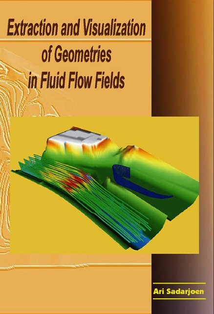
Extraction <strong>and</strong> <strong>Visualization</strong><br />
of Geometries<br />
in Fluid Flow Fields
About the cover background<br />
An embossed <strong>and</strong> rotated version of Colour Plate 6, which visualizes the Bay of<br />
Gdańsk (Pol<strong>and</strong>) using streamlines <strong>and</strong> vortices approximated by ellipses (see Section<br />
6.2). Data courtesy WL Delft Hydraulics.<br />
About the front cover<br />
A visualization of flow patterns in the harbour of Lith (The Netherl<strong>and</strong>s) <strong>and</strong> the Maas<br />
river, using particle paths coloured with the velocity magnitude (see Section 3.5.2).<br />
The colouring scheme uses a rainbow scale, with red showing the highest values <strong>and</strong><br />
blue the lowest values. The harbour (on the right) is separated from the river (on the<br />
left) by a thin dam, <strong>and</strong> contains a recirculation zone with much lower velocities than<br />
in the river. Data courtesy WL Delft Hydraulics.<br />
About the back cover<br />
Top image: transitional pipe flow, with vortices visualized by yellow ellipsoid icons<br />
<strong>and</strong> selective streamlines (see Section 6.3.4). Red shows streamlines in the left half<br />
of the pipe, white shows streamlines in the right half. Part of the cylinder wall with<br />
gridlines is shown in dark blue to increase the sense of depth. Data courtesy Lab. for<br />
Aero- <strong>and</strong> Hydrodynamics of Delft University of Technology.<br />
Middle image: flow past a tapered cylinder, with global streamlines in yellow <strong>and</strong><br />
vortices approximated by ellipses (see Section 4.5.2). The red ellipse indicates counterclockwise<br />
rotation, the green ellipse clockwise rotation. The background is a grid slice<br />
coloured (using the rainbow scale) with the scalar quantity, low values of which<br />
are supposed to indicate vortices. Data courtesy NASA Ames Research Center.<br />
Bottom image: flow in the Pacific Ocean, with the continent of North America shown<br />
in red. The figure shows streamlines coloured with the velocity magnitude (using<br />
the rainbow scale) <strong>and</strong> white curvature centre density peaks indicating vortices (see<br />
Section 4.3.2).<br />
Advanced School for Computing <strong>and</strong> Imaging<br />
This work was carried out in graduate school ASCI.<br />
ASCI dissertation series number 43.
Extraction <strong>and</strong> <strong>Visualization</strong><br />
of Geometries<br />
in Fluid Flow Fields<br />
PROEFSCHRIFT<br />
ter verkrijging van de graad van doctor<br />
aan de Technische Universiteit Delft<br />
op gezag van de Rector Magnificus prof.ir. K.F. Wakker<br />
in het openbaar te verdedigen ten overstaan van een commissie,<br />
door het College voor Promoties aangewezen,<br />
op ma<strong>and</strong>ag 12 april 1999 om 13:30 uur<br />
door<br />
Ignatius Armatessa SADARJOEN<br />
informatica ingenieur<br />
geboren te Mainz (Duitsl<strong>and</strong>)
Dit proefschrift is goedgekeurd door de promotor:<br />
Prof.dr.ir. F.W. Jansen<br />
Samenstelling promotiecommissie:<br />
Rector Magnificus, voorzitter<br />
Prof.dr.ir. F.W. Jansen, Technische Universiteit Delft, promotor<br />
Prof.dr.ir. C.J. van Duijn, Technische Universiteit Delft<br />
Prof.dr.ir. J. Biemond, Technische Universiteit Delft<br />
Prof.dr.ir. A.E. Mynett, IHE / WL Delft Hydraulics<br />
Prof.dr.ir. C.A. Grimbergen, Universiteit van Amsterdam<br />
Prof.dr. M. Rumpf, Universität Bonn<br />
Ir. F.H. Post heeft als begeleider in belangrijke mate aan de totst<strong>and</strong>koming van het<br />
proefschrift bijgedragen.<br />
CIP-DATA KONINKLIJKE BIBLIOTHEEK, DEN HAAG<br />
Sadarjoen, Ignatius Armatessa<br />
Extraction <strong>and</strong> <strong>Visualization</strong> of Geometries in Fluid Flow Fields / Ignatius Armatessa<br />
Sadarjoen . - [S.l. : s.n.]. Ill.<br />
Thesis Technische Universiteit Delft. - With ref. - With summary in Dutch.<br />
ISBN 90-6464012-2<br />
NUGI 855<br />
Subject heading: scientific visualization / computer graphics
Preface<br />
The research described in this thesis was conducted at the <strong>Computer</strong> <strong>Graphics</strong> <strong>and</strong><br />
CADCAM group of the Faculty of Information Technology <strong>and</strong> Systems of Delft University<br />
of Technology. It is the fourth in a series of PhD projects concerned with scientific<br />
visualization. The first to receive a PhD degree in visualization was Andrea<br />
Hin, who developed visualization techniques for turbulent flow [Hin, 1994]. A year<br />
later, Theo van Walsum graduated on the subject of selective visualization on curvilinear<br />
grids [van Walsum, 1995]. Next, Wim de Leeuw’s thesis described methods for<br />
presentation <strong>and</strong> exploration of flow data [de Leeuw, 1997]. All of these projects were<br />
concerned with visualization of fluid flows. My project continues along this line, although<br />
the focus is different: it concentrates on flow visualization using geometries, a<br />
collective name for curves, surfaces, <strong>and</strong> volumes.<br />
Many people have contributed to this dissertation, in many different ways <strong>and</strong><br />
degrees, some of whom I would like to thank in particular. The first <strong>and</strong> foremost<br />
figure I wish to thank is my supervisor Frits Post, who has had the largest influence<br />
on my work. His close involvement in my project has proven invaluable. During our<br />
frequent meetings <strong>and</strong> discussions, he was always full of new ideas <strong>and</strong> suggestions<br />
for me to try out (or ignore). When roads seemed a dead end, he always managed to<br />
fill me with his enthusiasm to find a way out, or to continue in other directions. I also<br />
greatly appreciate his thorough reading of <strong>and</strong> commenting on all my manuscripts,<br />
including this thesis.<br />
I thank my promotor Erik Jansen for offering me the opportunity to do this project<br />
in his group, for his enthusiastic support throughout the project, <strong>and</strong> in the final stage,<br />
for accurately yet quickly reading this manuscript.<br />
I want to thank some people from WL Delft Hydraulics, my co-supervisor Arthur<br />
Mynett, for his valuable time <strong>and</strong> comments <strong>and</strong> ideas provided during regular meetings,<br />
Jan Mooiman, for providing data sets <strong>and</strong> insights into their physical backgrounds,<br />
<strong>and</strong> Irving Elshoff, for his assistance in all matters related to AVS/Express<br />
<strong>and</strong> PLANKTON-97.<br />
I am also grateful to my new employers at the Manchester <strong>Visualization</strong> Centre<br />
for patiently having waited for me to finish my thesis full-time in Delft rather than<br />
part-time in Manchester.<br />
Two MSc students contributed to this PhD project. Ton van der Wouden designed<br />
<strong>and</strong> implemented CNX-lib, a well thought out library for unstructured grids.<br />
v
Alex de Boer reincarnated the PLANKTON particle tracer into PLANKTON-97 using<br />
AVS/Express, with several significant improvements.<br />
I would also like to thank Bing Ma from Tsinghua University in Beijing, who during<br />
his six-month stay in Delft provided me with data sets of the transient pipe flow <strong>and</strong> a<br />
wealth of background information.<br />
I am happy to have worked with David Banks from Mississippi State University,<br />
<strong>and</strong> Hans-Georg Pagendarm from the German Aerospace Centre, in a long-distance<br />
collaboration which formed the basis for a large part of <strong>Chapter</strong> 4 on vortex <strong>detection</strong>.<br />
The Knowledge Based Systems group of our Faculty kindly allowed me to use<br />
the Matlab package on their machines, which was indispensable for many of the 2D<br />
figures in this thesis.<br />
My office mate Freek extended his feature viewer to be (ab)used by me as a particle<br />
renderer, <strong>and</strong> contributed to an enjoyable work atmosphere through daily discussions<br />
(<strong>and</strong> distractions) about work <strong>and</strong> many other things. My other colleagues in<br />
the group, Alex, Erik, Klaas Jan, Marco, Maurice, Michal, Paul, (A.) Rafa, Theo, <strong>and</strong><br />
Winfried, also contributed to a pleasant work atmosphere, by regularly dropping into<br />
our office to show their exciting new results, <strong>and</strong> to guarantee the tea supply.<br />
The system administrators Aadjan, Kees, Peter, Piter, <strong>and</strong> last but certainly not<br />
least, Ruud, did their utmost to provide all the necessary hardware <strong>and</strong> software facilities.<br />
Non-technical but no less important support was provided by our secretaries<br />
Toos <strong>and</strong> Coby, “The Mothers” of the group.<br />
I am grateful to Mei-Ling Hsu, who looked up the Chinese originals of the poems<br />
decorating several chapter headings, <strong>and</strong> retyped them several times. Xièxiè! Evelien<br />
Rusch was so kind to look up the Swedish poems on very short notice, <strong>and</strong> type them<br />
in. Tack s˚a mycket!<br />
Erik Vullings, a PhD student in the Dept. of Electrical Engineering, had a significant<br />
influence on the course of my project, by providing me with useful technical <strong>and</strong><br />
procedural information.<br />
For the musical decoration during working hours, I would like to thank W.A. Mozart<br />
for composing such wonderful music, which always had a stimulating <strong>and</strong> refreshing<br />
effect, <strong>and</strong> which revitalized me whenever inspiration had run dry.<br />
I thank Driejana, who kept on encouraging me to finish soon <strong>and</strong> who helped to<br />
design the cover.<br />
Finally, I am grateful to my parents for all their love <strong>and</strong> unconditional support;<br />
without those, this work would not have been possible.<br />
vi<br />
I. Ari Sadarjoen
Contents<br />
1 Introduction 1<br />
1.1 Scientific visualization . ............................ 1<br />
1.2 Objectives . ................................... 2<br />
1.3 Structure of this thesis . ............................ 3<br />
2 Geometry extraction techniques 5<br />
2.1 Fields <strong>and</strong> grids . . . . . ............................ 6<br />
2.1.1 Fields ................................... 6<br />
2.1.2 Grids ................................... 6<br />
2.2 Curves . . . ................................... 8<br />
2.3 Surfaces . . ................................... 9<br />
2.3.1 Isosurfaces . . . . ............................ 10<br />
2.3.2 Stream surfaces . ............................ 10<br />
2.3.3 Implicit surfaces ............................ 12<br />
2.4 Deformable models ............................... 12<br />
2.4.1 Deformable curves . . . ........................ 13<br />
2.4.2 Deformable surfaces . . ........................ 15<br />
2.5 Vortices . . . ................................... 17<br />
3 Particle Tracing 21<br />
3.1 Fundamentals of particle tracing . . . .................... 21<br />
3.2 Particle tracing in curvilinear grids . . .................... 23<br />
3.2.1 Curvilinear grids ............................ 23<br />
3.2.2 Tetrahedral 5-decomposition . .................... 24<br />
3.3 Particle tracing in -transformed grids .................... 26<br />
3.3.1 -transformed grids . . ........................ 26<br />
3.3.2 Tetrahedral 6-decomposition . .................... 29<br />
3.4 Particle tracing in unstructured grids . .................... 33<br />
3.5 Examples . . ................................... 36<br />
3.5.1 A 3D backward-facing step . . .................... 36<br />
3.5.2 Lith Harbour . . ............................ 37<br />
3.5.3 A blunt fin . . . . ............................ 45<br />
vii
Contents<br />
3.6 Conclusions ................................... 45<br />
4 <strong>Vortex</strong> <strong>detection</strong> 47<br />
4.1 Physical vortex <strong>detection</strong> criteria . . . .................... 48<br />
4.1.1 Criteria descriptions . . ........................ 48<br />
4.1.2 Example . . . . . ............................ 49<br />
4.2 Critical points for vortex <strong>detection</strong> . . .................... 53<br />
4.3 The curvature centre method . ........................ 54<br />
4.3.1 Method description . . . ........................ 54<br />
4.3.2 Example . . . . . ............................ 56<br />
4.4 The enhanced curvature centre method . . . ................ 59<br />
4.4.1 Enhancements . . ............................ 59<br />
4.4.2 Example . . . . . ............................ 60<br />
4.4.3 Discussion . . . . ............................ 62<br />
4.5 The winding-angle method . . ........................ 64<br />
4.5.1 Method description . . . ........................ 65<br />
4.5.2 Example . . . . . ............................ 67<br />
4.6 Conclusions ................................... 69<br />
5 Deformable surfaces 71<br />
5.1 Surface definition <strong>and</strong> usage . . ........................ 71<br />
5.2 Initial surface creation . ............................ 73<br />
5.3 Surface deformation . . ............................ 75<br />
5.3.1 Node displacement . . . ........................ 77<br />
5.3.2 Fast node displacement ........................ 80<br />
5.4 Surface refinement . . . ............................ 81<br />
5.4.1 Refinement criteria . . . ........................ 82<br />
5.4.2 Refinement mechanisms ........................ 83<br />
5.5 Examples . . ................................... 85<br />
5.5.1 Extracting local isosurfaces . . .................... 85<br />
5.5.2 Extracting recirculation zones . .................... 88<br />
5.6 Conclusions ................................... 92<br />
6 Applications 93<br />
6.1 The Pacific Ocean . . . . ............................ 93<br />
6.1.1 Streamlines . . . ............................ 94<br />
6.1.2 <strong>Vortex</strong> <strong>detection</strong> with scalar criteria . ................ 94<br />
6.1.3 <strong>Vortex</strong> <strong>detection</strong> with critical points . ................ 95<br />
6.1.4 <strong>Vortex</strong> <strong>detection</strong> with curvature centres . . . . . . ......... 95<br />
6.1.5 <strong>Vortex</strong> <strong>detection</strong> with the winding-angle method ......... 97<br />
6.2 The Bay of Gdańsk ...............................100<br />
6.2.1 Particle tracing . ............................100<br />
6.2.2 <strong>Vortex</strong> <strong>detection</strong> with scalar criteria . ................100<br />
6.2.3 <strong>Vortex</strong> <strong>detection</strong> with critical points . ................102<br />
viii
Contents<br />
6.2.4 <strong>Vortex</strong> <strong>detection</strong> with curvature centres . . . . . . .........106<br />
6.2.5 <strong>Vortex</strong> <strong>detection</strong> with the winding-angle method .........108<br />
6.3 A transitional pipe flow ............................109<br />
6.3.1 Particle tracing . ............................109<br />
6.3.2 <strong>Vortex</strong> <strong>detection</strong> with the winding-angle method ......... 112<br />
6.3.3 <strong>Vortex</strong> <strong>detection</strong> with scalar criteria . ................ 112<br />
6.3.4 <strong>Vortex</strong> <strong>detection</strong> with selective <strong>and</strong> iconic techniques . . ..... 116<br />
6.4 The Delta-Wing aircraft . ............................ 118<br />
6.4.1 Particle tracing . ............................ 118<br />
6.4.2 <strong>Vortex</strong> <strong>detection</strong> using deformable surfaces . . . . ......... 118<br />
7 Conclusions <strong>and</strong> future work 123<br />
7.1 Conclusions ...................................123<br />
7.2 Future work ...................................125<br />
Bibliography 127<br />
Colour Plates 135<br />
Summary 143<br />
Samenvatting 145<br />
Curriculum Vitæ 147<br />
ix
<strong>Chapter</strong> 1<br />
Introduction<br />
1.1 Scientific visualization<br />
Salt, bittersalt 1<br />
är havet, och klart och kallt.<br />
P˚a djupet multnar mycket,<br />
men havet renar allt.<br />
Scientific visualization could be described as the art of translating numbers into a clear<br />
visual representation, which makes it easier for people to interpret the numbers. Scientific<br />
visualization has a long history: an early well-known example dates back from<br />
1861, when Charles Joseph Minard created an ingenious graphical representation of<br />
numerical multidimensional data concerning Napoleon’s unsuccessful campaign to<br />
Russia in 1812–1813. This visualization is shown in Figure 1.1 [Tufte, 1990]. The chart<br />
visualizes the size of Napoleon’s army which is dramatically reduced as the campaign<br />
proceeds through various locations. On the way to Moscow, indicated by the hatched<br />
b<strong>and</strong>, the army size decreases from 422,000 to 100,000. On the way back, indicated<br />
by the solid black b<strong>and</strong>, the army is literally decimated to 10,000. This graph visualizes<br />
six variables: the army position (longitude <strong>and</strong> latitude), its size, its direction of<br />
movement, the temperature, <strong>and</strong> the date.<br />
Before the advent of computers, scientists who conducted experiments also developed<br />
ways of visualizing the results. Many of you may remember from the science<br />
classes in high school that magnetic field lines can be visualized by iron shavings,<br />
which are oriented when a magnet is put under a sheet of paper. A slightly more advanced<br />
way of visualization is the use of aluminium particles released in a flow <strong>and</strong><br />
photographed at regular intervals.<br />
In modern times, scientific research <strong>and</strong> engineering practice increasingly employ<br />
computer simulations <strong>and</strong> automatic measurements, which result in large amounts<br />
of numbers. Simulations are performed by scientists for modelling complex physical<br />
phenomena, about which they try to get a better underst<strong>and</strong>ing. Simulations are also<br />
performed by engineers who want to test <strong>and</strong> improve their designs, without having<br />
to build costly prototypes or scale models. Measurements are often taken in large<br />
amounts by satellites, which orbit the earth or are sent out to other planets in the solar<br />
system. These computer simulations <strong>and</strong> measurements produce large amounts of<br />
data, called data sets, typically in the form of numbers. As the power of computers has<br />
steadily increased over the years, this has allowed scientists <strong>and</strong> engineers to develop<br />
1Salt, bitter salt // is the sea, <strong>and</strong> clear <strong>and</strong> cold // In the deep, much decays // but the sea cleans<br />
everything. (Karin Boye: Havet)<br />
1
<strong>Chapter</strong> 1. Introduction<br />
Figure 1.1: Minard’s visualization of Napoleon’s campaign to Russia [Tufte, 1990]<br />
more complex <strong>and</strong> more accurate models that produce larger <strong>and</strong> larger data sets,<br />
which have to be visualized.<br />
Therefore, scientific visualization has become necessary for scientists <strong>and</strong> engineers,<br />
in order to obtain insight in the results of their models <strong>and</strong> measurements. Images<br />
are much better suited for processing by the human visual system, hence the<br />
well-known proverb “One picture says more than a thous<strong>and</strong> words” (or numbers in this<br />
case).<br />
1.2 Objectives<br />
The research in this thesis describes the development of techniques to assist the scientific<br />
user in coping with the large amounts <strong>and</strong> high complexity of the data, by<br />
providing interactive techniques for exploring the data. What the user is usually interested<br />
in, are the characteristic phenomena of the data, so-called features. Examples<br />
of features are vortices, boundary layers, <strong>and</strong> shock waves. Through these features,<br />
the amount of data <strong>and</strong> its complexity can be reduced. Therefore, we have developed<br />
techniques which extract features from data sets <strong>and</strong> visualize them.<br />
One classification for visualization techniques distinguishes between: global techniques,<br />
geometric techniques, <strong>and</strong> feature-based techniques [Post et al., 1999]. Global<br />
techniques render data directly, without deriving curves or polygons first. Global techniques<br />
include arrow plots, direct volume rendering, <strong>and</strong> direct surface rendering. An<br />
2
1.3. Structure of this thesis<br />
advanced global technique, which uses texture to visualize vector fields, is Spot Noise<br />
[de Leeuw, 1997]. Geometric techniques first extract geometric objects, such as curves, surfaces<br />
<strong>and</strong> solids, <strong>and</strong> then render them for visualization. Examples are streamlines <strong>and</strong><br />
stream surfaces. Feature-based techniques first extract features <strong>and</strong> then visualize them<br />
with any of the previous techniques or with abstract iconic representations. Examples<br />
of the latter are given in [van Walsum et al., 1996].<br />
The focus in this thesis is on geometric techniques, although sometimes we employ<br />
elements from feature-based techniques as well. An important reason is that geometries<br />
are easy to perceive <strong>and</strong> easy to render. This leads to the main objective of this<br />
thesis:<br />
to describe techniques for extracting <strong>and</strong> visualizing geometries in fluid flow fields.<br />
The application area in this thesis is fluid flows, both hydrodynamic <strong>and</strong> aerodynamic,<br />
because this area contains a wealth of interesting problems, <strong>and</strong> because we had access<br />
to experts <strong>and</strong> resources in that area. Within this field, we concentrated on Computational<br />
Fluid Dynamics (CFD), the field which develops numerical models of fluid flows<br />
<strong>and</strong> performs flow simulations based upon those models.<br />
1.3 Structure of this thesis<br />
The remainder of this thesis has the following structure. <strong>Chapter</strong> 2 contains an overview<br />
of related work in geometric techniques, <strong>and</strong> serves as a framework for placing the<br />
techniques covered in the following chapters into context. <strong>Chapter</strong> 3 describes particle<br />
tracing, a technique for visualizing velocity fields. <strong>Chapter</strong> 4 covers techniques for<br />
detecting vortices. <strong>Chapter</strong> 5 investigates deformable surfaces, a class of geometric objects<br />
that can be used for extracting a range of features which may be well represented<br />
by surfaces. <strong>Chapter</strong> 6 presents some applications of the techniques to some larger,<br />
‘real-life’ examples. Finally, <strong>Chapter</strong> 7 contains conclusions <strong>and</strong> gives directions for<br />
future work.<br />
3
<strong>Chapter</strong> 2<br />
Geometry extraction techniques<br />
Bengawan Solo, . . . 1<br />
Mata airmu dari Solo<br />
terkurung gunung seribu<br />
Air mengalir sampai jauh<br />
akhirnya ke laut.<br />
This chapter reviews related work concerning geometry extraction. The purposes of<br />
this chapter are to show the context of our work <strong>and</strong> to provide a basis for the discussions<br />
in the following chapters.<br />
As stated in <strong>Chapter</strong> 1, it is possibly to classify visualization techniques as direct<br />
techniques, geometric techniques, <strong>and</strong> feature-based techniques [Post et al., 1999]. The<br />
focus in this thesis is on geometric techniques, although sometimes we employ elements<br />
from feature-based techniques as well. Geometric techniques produce geometries,<br />
which have two important advantages:<br />
¯ geometries are easy for people to interpret. The visual system of the human<br />
brain is well adapted to recognizing shapes <strong>and</strong> colour properties of geometries<br />
like surfaces <strong>and</strong> curves.<br />
¯ geometries are easy for computers to display. Modern hardware systems of computers<br />
are specialized in rendering lines <strong>and</strong> surfaces with colours <strong>and</strong> textures,<br />
to create a clear representation.<br />
Several important types of geometries are:<br />
¯ curves<br />
¯ surfaces<br />
¯ solids<br />
¯ deformable models<br />
Curves are often used to get a global view of the flow field. Surfaces are often used<br />
to get a local view of specific surface features, such as stream surfaces or separation<br />
surfaces. Deformable models are a special type of curves <strong>and</strong> surfaces, which start<br />
from some initial shape, <strong>and</strong> grow or shrink towards some target shape of a feature. In<br />
addition, a vortex is not a type of geometry, but a type of feature in fluid flows, which<br />
may be represented by various types of geometries, such as curves <strong>and</strong> surfaces.<br />
The remainder of this chapter is organized as follows. Section 2.1 gives definitions<br />
of several kinds of data fields <strong>and</strong> grids. Section 2.2 describes various flow curves,<br />
1 Solo River, ...//Yoursource is in Solo // confined by a thous<strong>and</strong> mountains // Your water flows quite<br />
far // <strong>and</strong> finally into the sea. (Indonesian traditional)<br />
5
<strong>Chapter</strong> 2. Geometry extraction techniques<br />
<strong>and</strong> Section 2.3 various flow surfaces. Section 2.4 covers deformable models. Finally,<br />
Section 2.5 describes techniques for vortex <strong>detection</strong>.<br />
2.1 Fields <strong>and</strong> grids<br />
2.1.1 Fields<br />
A three-dimensional field can be represented analytically by a global function Ü Ý Þ ,<br />
defined over a bounded spatial domain in Ê [Silver et al., 1999]. A unique field value<br />
× at every point Ü Ý Þ of the domain can be found by evaluation: × Ü Ý Þ everywhere<br />
in the domain. This is usually not the case with the discrete numerical fields<br />
that are more common in science <strong>and</strong> engineering, where data values are known only<br />
at a finite number of data points. Such discrete fields are usually generated by data<br />
acquisition systems or numerical computer simulations.<br />
Measured data fields can be generated by medical imaging systems, such as computed<br />
tomography (CT), magnetic resonance imaging (MRI), or positron emission tomography<br />
(PET) scanners. Other sources of large measured data fields include remote<br />
sensing systems of satellites, scanning electron microscopes, <strong>and</strong> seismic <strong>and</strong> acoustic<br />
sensing for underwater observations. For simplicity, we will assume in the rest of this<br />
thesis that the data fields have been generated by numerical simulations.<br />
Physical models often consist of partial differential equations that cannot be solved<br />
globally <strong>and</strong> analytically. Therefore, discrete methods such as finite elements, finite<br />
differences, or finite volume methods are often used to numerically solve local equations.<br />
These methods are based on defining a computational grid, consisting of nodes<br />
<strong>and</strong> cells. Approximated equations are specified, resulting in a system of equations<br />
that can be solved numerically at each grid node or cell.<br />
The domain of a simulation may have two or three spatial dimensions. It may also<br />
be varying in time. The data points (or grid points) thus are 2D Ü Ý or 3D Ü Ý Þ<br />
coordinate positions. The data fields may contain any combination of scalar quantities<br />
(e.g. pressure, density, or temperature), vector quantities (e.g. force or velocity), or<br />
tensor quantities (e.g. stress or deformation) at each data point. The data values may<br />
be constant in time, or vary as a function of time. Time-dependent fields are important<br />
for highly dynamic phenomena such as fluid flow.<br />
2.1.2 Grids<br />
There are many types of computational grids, depending on the simulation technique,<br />
the domain, <strong>and</strong> the application [Silver et al., 1999]. A grid consists of nodes <strong>and</strong> cells.<br />
The nodes are points defined in the simulation domain, <strong>and</strong> the cells are simple spatial<br />
elements connecting the nodes: triangles or quadrangles in 2D, tetrahedra or hexahedra<br />
in 3D. The cells must fill the whole domain, but may not intersect or overlap, <strong>and</strong><br />
adjacent cells must have common edges <strong>and</strong> faces. Grids can be classified according to<br />
6
2.1. Fields <strong>and</strong> grids<br />
their geometry, their topology, <strong>and</strong> their cell shape. Three of the most important types<br />
are discussed below.<br />
The simplest type is the uniform grid, also called regular orthogonal, or Cartesian<br />
grid (see Figure 2.1a). This type of grid has a regular geometry <strong>and</strong> topology: the<br />
nodes are spaced in a regular array, <strong>and</strong> the cells are all unit cubes. The grid lines<br />
connecting the nodes are straight <strong>and</strong> orthogonal. Every node can be referenced by<br />
integer indices . Adjacent nodes can be found by incrementing any of the index<br />
vector components. Many operations on this type of grid (such as searching the<br />
grid cell which contains a given point) are very simple, but grid resolution is constant<br />
throughout the domain, <strong>and</strong> the shape of the domain must be rectangular.<br />
(a) (c)<br />
(b)<br />
Figure 2.1: Several grid types: (a) regular orthogonal (Cartesian) grid, (b) structured<br />
curvilinear grid, <strong>and</strong> (c) unstructured grid<br />
The second type of grid is the structured curvilinear grid (see Figure 2.1b). This type<br />
has a regular topology (the adjacency pattern for each internal node is the same), with<br />
the nodes again referenced by integer indices , <strong>and</strong> adjacent nodes can be found<br />
7
<strong>Chapter</strong> 2. Geometry extraction techniques<br />
by incrementing index values. The cells are usually hexahedra, with a deformed-brick<br />
shape. The geometry of each cell is irregular, <strong>and</strong> the cell faces are non-planar quadrangles.<br />
The cell size of a curvilinear grid can be highly variable, <strong>and</strong> thus the resolution<br />
of the simulation can be higher in areas of strong variation. Also, the curvilinear shape<br />
can be made to conform to the boundary of a curved object, such as an airplane wing.<br />
This type of grid is common in finite volume CFD simulations.<br />
The third type of grid is the unstructured grid, where the topology <strong>and</strong> geometry<br />
are both irregular. Figure 2.1c shows an example from a finite element application<br />
[van den Broek et al., 1998]. The nodes do not have a fixed adjacency pattern, <strong>and</strong><br />
adjacency information cannot be derived from a spatial index, but has to be stored<br />
explicitly. The cells are usually triangles in 2D or tetrahedra in 3D. Cell size can be<br />
varied according to the amount of detail desired, <strong>and</strong> can be used to model a complex<br />
geometry. Unstructured grids are often used in finite element analysis. Due to the<br />
simple cell geometry, calculations on a single cell are simple.<br />
There are many more variations of grids: staggered grids, hybrid (mixed-type)<br />
grids, multi-block grids, moving grids, <strong>and</strong> multi-resolution grids. In this thesis, we<br />
will concentrate mainly on the three types described before.<br />
A numerical simulation will generally produce a discrete data field, consisting of<br />
a combination of scalar, vector, or tensor quantities, given at every grid node. These<br />
datasets can be very large, with as many as to nodes, <strong>and</strong> ten or more variables<br />
defined at every node. This can result in a size of up to hundreds of megabytes for<br />
stationary (time-independent) fields <strong>and</strong> up to terabytes for time-dependent fields.<br />
2.2 Curves<br />
Curves are usually easy to generate, easy to render, <strong>and</strong> easy to underst<strong>and</strong>. An important<br />
subclass of curves are flow curves, which are used to visualize flow patterns.<br />
The definitions of several flow curves are listed below [Silver et al., 1999].<br />
¯ streamline: a tangent curve of a steady velocity field. Tangent curves are defined<br />
as curves that are everywhere tangent to the vector field. A streamline satisfies<br />
the equations: ÜÙ ÝÚ ÞÛ, where Ù Ú Û are the velocity components<br />
in the Ü-, Ý-, <strong>and</strong> Þ-direction of the domain.<br />
¯ pathline: a trajectory curve of a single fluid particle moving in the flow. This curve<br />
is identical to an integral curve obtained by stepwise integration of the velocity<br />
vector field (see <strong>Chapter</strong> 3 on the generation of pathlines).<br />
¯ streak line: a line joining the positions at one instant of all particles that have been<br />
released from a single point over a given time interval Ø ØÒ.<br />
¯ time line: a line connecting all particles that have been simultaneously released in<br />
a flow from positions on a straight line, perpendicular to the flow direction. The<br />
straight line moves <strong>and</strong> deforms with the flow due to local velocity variations.<br />
¯ vorticity line: a tangent curve of a vorticity vector field, which is the curl of velocity<br />
field: Ö¢Ú.<br />
8
2.3. Surfaces<br />
¯ hyperstreamline: a tangent curve of an eigenvector (usually with the largest magnitude)<br />
of a tensor field [Delmarcelle & Hesselink, 1993].<br />
In a steady flow (also called stationary or time-independent flow), where the velocity<br />
field is constant in time, pathlines, streamlines, <strong>and</strong> streak lines are identical [Strid<br />
et al., 1989]. In an unsteady flow (also called instationary or time-dependent flow),<br />
these curves may all be different. Streamlines, vorticity lines, <strong>and</strong> hyperstreamlines<br />
are mathematical abstractions, but they are all based on the idea of field lines. Many<br />
of these curves have been inspired by experimental visualization [Post & van Walsum,<br />
1993].<br />
Most of the curves are based on the notion of particle advection. They can be generated<br />
in a straightforward way, by integrating the vector field, which results in an<br />
integral curve. Particle tracing is a visualization method which simulates the release<br />
of massless particles, calculates their paths, <strong>and</strong> then renders them in an animation at<br />
a constant frame rate. Particle tracing is a common way of visualizing the results of<br />
CFD flow simulations; an extension for turbulent flow was introduced in [Hin & Post,<br />
1993; Hin, 1994].<br />
The choice of release points for particles or flow curves is critical. If flow curves<br />
are released too sparsely, or in the wrong regions, important flow features may be<br />
missed. If they are released too densely, cluttering may occur. An important technique<br />
for an even distribution of the lines is described in [Turk & Banks, 1996]. Recently, this<br />
technique was extended to curvilinear grids [Mao et al., 1998].<br />
Effectively rendering 3D curves is much more difficult than rendering 2D curves,<br />
due to occlusion, <strong>and</strong> the lack of direction information <strong>and</strong> depth cues. In [Fuhrmann<br />
&Gröller, 1998], some solutions are proposed, such as an algorithm for an even distribution<br />
of curves, <strong>and</strong> the use of texture for depth cues.<br />
Our focus in this thesis is on the calculation of pathlines, or particle tracing in special<br />
grid types: in structured curvilinear grids (see Section 3.2), in -transformed grids,<br />
which are common in hydrodynamic applications (see Section 3.3), <strong>and</strong> in unstructured<br />
grids, which are more common in aerodynamics (see Section 3.4).<br />
2.3 Surfaces<br />
Curves are easy to visualize, but they do not carry much spatial information, <strong>and</strong> are<br />
therefore difficult to locate visually in space [Post & van Walsum, 1993]. Surfaces are<br />
much better for visualization, because lighting <strong>and</strong> shading are effective cues for perception<br />
of 3D shapes by a human observer.<br />
Our focus in this thesis is on the generation of flow surfaces of three kinds. The<br />
first kind is adaptive isosurfaces, which can be used to approximate local isosurfaces<br />
with the desired accuracy specified by the user (see Section 5.5.1). The second kind is<br />
separation surfaces (see Section 5.5.2), which are used to find recirculation zones. The<br />
third kind is vortex tubes (see Section 6.4). For completeness, a brief introduction to<br />
isosurfaces, stream surfaces, <strong>and</strong> implicit surfaces is given below.<br />
9
<strong>Chapter</strong> 2. Geometry extraction techniques<br />
2.3.1 Isosurfaces<br />
An isosurface is a collection of points Ü Ý Þ in a scalar field Ü Ý Þ which have<br />
the same field value: Ü Ý Þ , where is a constant value called the isovalue.<br />
These points are usually connected by a polygon surface. The classic algorithm to<br />
generate isosurfaces is the marching cubes algorithm described in [Lorensen & Cline,<br />
1987]. Based on this algorithm, many improvements, optimizations, <strong>and</strong> variations<br />
have been produced, but these do not fall within the scope of this thesis.<br />
While isosurfaces are certainly useful for extracting certain types of features from<br />
data sets, they also have drawbacks. St<strong>and</strong>ard isosurface algorithms work with a<br />
global isovalue, which may lead to surface fragments throughout the entire data set.<br />
This may not always be desirable, when we are only interested in a certain region<br />
of interest. Another drawback is that st<strong>and</strong>ard algorithms generate large amounts of<br />
polygons, which has a strong relation to the number of grid cells. Sometimes, this is<br />
reduced afterwards with the use of surface simplification or decimation algorithms, at<br />
the cost of extra processing time.<br />
A better option would be to prevent too many polygons from being generated in<br />
the first place. Ideally, one would want to start from a coarse surface, <strong>and</strong> progressively<br />
refine it, when <strong>and</strong> as long as necessary. This approach has been followed in [Grosso<br />
& Ertl, 1998].<br />
Our deformable surfaces, as described in Section 5.5.1, are also usable for generating<br />
progressive isosurfaces with adaptive precision.<br />
2.3.2 Stream surfaces<br />
The flow curves in 2D data fields, as defined in Section 2.2, can be extended to flow<br />
surfaces in 3D data fields. For stationary vector fields in general, the tangent curve is<br />
extended to a tangent surface, a surface that is everywhere tangent to the vector direction.<br />
For stationary velocity fields, a tangent surface is called a stream surface. As the<br />
velocity direction is everywhere tangent to the stream surface, the velocity component<br />
normal to the surface is everywhere zero. This means that no material flows through a<br />
stream surface, so it can be considered as a separation between two independent flow<br />
zones.<br />
The simplest type of stream surface is a ribbon, or a narrow b<strong>and</strong>. Besides local<br />
flow direction, it can show the local rotation of the flow. Ribbons can be generated<br />
in different ways [Pagendarm & Post, 1997]. First, two adjacent streamlines can be<br />
generated from two seed points placed close together, <strong>and</strong> constructing a mesh of triangles<br />
between them. The width of the ribbon depends on the distance between the<br />
trajectories of both streamlines, <strong>and</strong> may become large in a strongly divergent area. A<br />
second way is to construct a surface strip of constant width centered around a single<br />
streamline. The orientation of the strip is directly linked to the angular velocity of the<br />
flow, obtained from the vorticity . From the angular velocity, a rotation angle can<br />
be found by time integration along the streamline [Pagendarm & Walter, 1994]. The<br />
initial orientation is defined at the seed point, <strong>and</strong> an incremental rotation is applied<br />
10
2.3. Surfaces<br />
in a local coordinate frame at each point on the streamline. The ribbon is constructed<br />
by weaving a strip of triangles between the points.<br />
Both methods for creating ribbons have advantages [Pagendarm & Post, 1997]. The<br />
first method can show vortical behaviour of the flow, but can also show other effects as<br />
well. For instance, it will also show divergence, through the varying width of the ribbon.<br />
The second method shows purely local vortical behaviour on the central streamline.<br />
In both cases, the surface is not an exact stream surface, as the tangency condition<br />
is only true for the constructing streamlines.<br />
A general stream surface can be constructed by generating streamlines from each<br />
of a number of points on an initial line segment or rake. If for all these streamlines a<br />
single constant time step is used, then the lines connecting points of equal time on all<br />
streamlines are time lines. Streamlines <strong>and</strong> time lines thus make a quadrangular mesh<br />
(see Figure 2.2a), which can be easily divided into triangles for visualization.<br />
rake<br />
time line<br />
streamline<br />
(a) Mesh for stream surface, with<br />
streamlines from a rake, <strong>and</strong> timelines<br />
Figure 2.2: Stream surface generation<br />
(b) Divergent flow<br />
splits a stream surface<br />
This st<strong>and</strong>ard algorithm has some disadvantages. If the flow is strongly divergent,<br />
adjacent streamlines will move too far apart. If there is an object in the flow, the surface<br />
must be split, <strong>and</strong> this is problematic with the st<strong>and</strong>ard algorithm (see Figure 2.2b). Finally,<br />
if there are high velocity gradients in the flow direction, the mesh will be strongly<br />
distorted <strong>and</strong> unequal-sized <strong>and</strong> poorly-shaped triangles will result.<br />
To solve these problems, an ‘advancing front’ algorithm has been proposed<br />
[Hultquist, 1992]. The surface is generated in the transverse direction by adding a<br />
strip of triangles to the front. Using adaptive time steps to compensate the gradients<br />
in the flow direction, all points at the front will move forward by about the same distance.<br />
Also, if two adjacent points on the front move too far apart by divergence, a new<br />
streamline is started at the midpoint between them. Conversely, if two points move<br />
too close together, one streamline is terminated. If an object in the flow is detected, the<br />
front can be split, <strong>and</strong> the two parts can move on separately.<br />
Stream surfaces can also be used to generate streamlines [Kenwright & Mallinson,<br />
1992a]. Two local stream surfaces are determined from dual stream functions defined<br />
11
<strong>Chapter</strong> 2. Geometry extraction techniques<br />
in a grid cell. The intersection curve of these stream surfaces is a streamline segment,<br />
which is approximated by determining the entry <strong>and</strong> exit points of the streamline segment<br />
in the cell, <strong>and</strong> connecting these points. A stream line is constructed by tracking<br />
from a starting point through the cells. This technique is very different from the time<br />
stepping integration techniques described in Section 3.1, <strong>and</strong> has the advantage of conforming<br />
with the physical law of mass conservation.<br />
2.3.3 Implicit surfaces<br />
Two important approaches to mathematically define curves <strong>and</strong> surfaces are parametric<br />
<strong>and</strong> implicit [Bloomenthal, 1997]. The parametric approach defines each of the coordinates<br />
as an explicit function of one or more parameters. For a 2D surface in 3D space,<br />
these functions are: Ü Ü × Ø Ý Ý × Ø , <strong>and</strong> Þ Þ × Ø , when × Ø is an ordered<br />
pair of parameters. In the implicit approach, the coordinates Ü Ý Þ are not given<br />
explicitly, but as the set of points Ü Ý Þ Ü Ý Þ , where is some constant.<br />
Then, Ü Ý Þ is a surface implicitly defined by , oranimplicit surface, <strong>and</strong> depending<br />
on the form of , other values of the constant indicate the distance to the<br />
surface. An example is the spherical surface given by Ü Ý Þ .<br />
Implicit surfaces can be used to generate stream surfaces [van Wijk, 1993]. The<br />
stream surface must satisfy the condition Ö ¡ Ú , which means that the normal to<br />
the surface (denoted by the gradient Ö) is perpendicular to the velocity direction. The<br />
function is called the stream surface function. The values of are specified at the inflow<br />
boundaries of the flow area, <strong>and</strong> for all other grid points the values of are calculated<br />
numerically. This can be done in two ways: by solving the convection equation, <strong>and</strong><br />
by tracing backwards from each grid point to the inflow boundary. A stream surface<br />
is then generated as an isosurface of . This technique can also be adapted to generate<br />
time surfaces.<br />
There are two problems with implicit surfaces: it is difficult to specify <strong>and</strong> control<br />
their shape, <strong>and</strong> it is difficult to sample them uniformly. One solution to these<br />
problems, described in [Witkin & Heckbert, 1994], works by placing particles on the<br />
surface. Constraints are imposed on the surface <strong>and</strong> the particles for two purposes:<br />
first, it makes the surface follow the particles when they are moved. In this way, the<br />
user can control the shape by interactively moving the particles, <strong>and</strong> the surface will<br />
adapt its shape. Second, when the constraint is used in the other direction, it makes<br />
the particles follow the surface. In that way, when the surface shape is changed, the<br />
particles, which are floating but restricted to the surface, will evenly redistribute themselves<br />
over the surface. Note that this is a type of surface consisting of independent<br />
points, not connected by edges <strong>and</strong> polygon faces.<br />
2.4 Deformable models<br />
A special class of geometries, which includes both curves <strong>and</strong> surfaces, is formed by<br />
what we call deformable models, geometries which all have in common that they start<br />
12
2.4. Deformable models<br />
from some initial shape, <strong>and</strong> are deformed in an iterative process to some target shape.<br />
This target shape is usually some object in a 2D or 3D image.<br />
The advantage of deformable models is that they allow for the extraction of features<br />
which cannot be expressed as isosurfaces, but for which optimization criteria are<br />
easy to specify, e.g. curves or surfaces which are located at local gradient maxima. By<br />
utilizing a priori knowledge, deformable models may be given properties which isosurfaces<br />
do not have. For example, deformable models may be prescribed to have a<br />
certain topology, while the topology of a collection of isosurface polygons is usually<br />
unpredictable.<br />
Basically, there are three types of deformable models: deformable curves, deformable<br />
surfaces, <strong>and</strong> deformable volumes. Deformable curves are curves in 2D space, deformable<br />
surfaces are surfaces in 3D space, <strong>and</strong> deformable volumes are solid objects in 3D<br />
space. The essential difference between deformable surfaces <strong>and</strong> deformable volumes<br />
is that the latter can also represent the internal structure of the domain.<br />
Deformable models have been applied in various areas, such as image processing,<br />
medical imaging, <strong>and</strong> computer graphics. For a good <strong>and</strong> recent textbook on deformable<br />
models, which covers applications in these three areas, see [Metaxas, 1997].<br />
For a recent survey of the use of deformable models in medical imaging, see [McInerney<br />
& Terzopoulos, 1996].<br />
We have developed a type of deformable surfaces for a totally different application<br />
area: <strong>detection</strong> of surface features in fluid flows. This will be described in <strong>Chapter</strong> 5<br />
of this thesis. Since our technique has most in common with deformable curves <strong>and</strong><br />
surfaces, the remainder of this section will describe related work on deformable curves<br />
(see Section 2.4.1) <strong>and</strong> deformable surfaces (see Section 2.4.2).<br />
2.4.1 Deformable curves<br />
Deformable curves were first proposed in [Kass et al., 1988] for object segmentation<br />
in image processing applications. Typically, the user defines an initial curve, in the<br />
neighbourhood of the target object to be segmented. The user may put constraints on<br />
some points, e.g. by anchoring them to fixed points, or by attaching springs between<br />
different points. Then, a minimization process of the curve energy causes the snake to<br />
be gradually attracted to the contour of the object. Due to their shape <strong>and</strong> wiggling<br />
behaviour, these curves were called “snakes”.<br />
In [Kass et al., 1988], snakes were defined as “energy-minimizing splines guided by<br />
external constraint forces <strong>and</strong> influenced by image forces that pull them toward features<br />
such as lines <strong>and</strong> edges”. The energy of a snake, which is defined as a parametric<br />
curve with parameter ×, is defined in [Kass et al., 1988] as:<br />
£ ×Ò<br />
<br />
<br />
<br />
<br />
×Ò Ú × ×<br />
ÒØ Ú × × Ñ Ú × × ÓÒ Ú × × (2.1)<br />
13
<strong>Chapter</strong> 2. Geometry extraction techniques<br />
where Ú × Ü × Ý × are the positions of the snake elements as a function of the<br />
curve parameter ×, ÒØ is the internal spline energy, Ñ is the image energy which<br />
causes a snake to be attracted to images features, <strong>and</strong> ÓÒ is the constraint energy<br />
imposed by the user.<br />
The internal energy ÒØ, which controls the continuity of a snake, is defined as a<br />
weighted average: ÒØ « × Ú× × ¬ × Ú×× × . It consists of a first-order<br />
derivative term Ú× × <strong>and</strong> a second-order derivative term Ú×× × . The first term makes<br />
the snake first-order continuous, the second makes it second-order continuous, with<br />
« × <strong>and</strong> ¬ × determining the weight of each term. If ¬ × , the snake is secondorder<br />
discontinuous.<br />
The image energy Ñ causes the snake to be attracted to lines, edges, <strong>and</strong><br />
(line segment) terminations, <strong>and</strong> is also defined as a weighted average: Ñ <br />
ÛÐÒÐÒ Û ÛØÖÑØÖÑ.<br />
The last term of the snake energy, the constraint energy ÓÒ, allows the user to<br />
fix certain points of a snake to the background, or to connect two points of adjacent<br />
snakes to each other with a spring. If two points have coordinates Ü <strong>and</strong> Ü , then<br />
a spring between those two points could add a term Ü Ü to the constraint<br />
energy, where is the stiffness of the spring.<br />
When all the energy terms have been defined <strong>and</strong> substituted in the total energy<br />
(2.1), the energy is minimized by a variational calculus approach. This basically means<br />
that new snake positions are calculated as small variations of the old ones, such that<br />
the energy gradually decreases at each iteration, <strong>and</strong> ultimately is minimized. This<br />
will cause an initial snake defined around an object to shrink <strong>and</strong> lock onto the actual<br />
object contour.<br />
The snakes article has been the basis for numerous other types of deformable<br />
curves. One further development were the fast active contours described in [Williams<br />
& Shah, 1990]. There are several differences with the original snakes. One difference<br />
is that the calculations are not done in continuous Ê space, but on a discrete grid of<br />
pixels, which makes sense for image processing applications. Another difference with<br />
the original snakes is the use of a greedy algorithm to compute new positions of snake<br />
elements. For each of the neighbour pixels of a snake element, the greedy algorithm<br />
calculates the effect of moving that element to that pixel on the new energy of the entire<br />
contour. The algorithm then moves each element to the neighbour pixel which leads<br />
to the lowest energy. One of the advantages of the greedy algorithm is that it works<br />
much faster than variational calculus.<br />
Yet another type of deformable curves is the Discrete Dynamic Contours described in<br />
[Lobregt & Viergever, 1995]. Like previous models, they are based on minimization of<br />
an energy, composed of external energy related to image features, <strong>and</strong> internal energy<br />
related to local curvature. In this case, the energy is not minimized by variational<br />
calculus or a greedy algorithm, but by means of forces, which are used in Newtonian<br />
motion equations to determine the new positions of the nodes. The force on a node <br />
is given by:<br />
ÛÜ ÜÖ ÛÒ Ò ÑÔ (2.2)<br />
14
2.4. Deformable models<br />
where ÜÖ is the radial component (in the direction Ö) of an external force, with an<br />
associated weight, Ò is an internal force, with an associated weight, <strong>and</strong> ÑÔ is a<br />
damping force which increases the stability <strong>and</strong> ensures termination of the iteration.<br />
From these forces, the acceleration for the nodes is easily derived using the relation<br />
Ñ, where is Ñ is a constant mass for all nodes. From the acceleration, the<br />
velocity is derived, <strong>and</strong> using the velocity, the new position Ô of a node is determined<br />
using a numerical integration:<br />
Ô Ø ¡Ø Ô Ø Ú Ø ¡Ø (2.3)<br />
where ¡Ø is the time interval between subsequent new positions.<br />
There are several important differences between Discrete Dynamic Contours (DDC)<br />
<strong>and</strong> previous models.<br />
1. The first difference is that in DDCs, minimization of the energy is done for each<br />
individual node, not globally for the entire contour, hence the name discrete.<br />
2. The second difference is that displacement of the nodes is done only in the radial<br />
direction, or the direction normal to the contour, filtering out any tangential displacement<br />
components. This is done for two reasons: tangential displacements<br />
do not contribute to deformation of the model, <strong>and</strong> tangential displacements<br />
may cause local accumulation of nodes on the contour, which is not desirable.<br />
3. The third important difference is that DDCs perform resampling of the curve<br />
<strong>and</strong> add new nodes, which can make the final contour much larger than the one<br />
originally defined.<br />
In principle, deformable contours are limited to 2D images, or 2D slices of 3D<br />
data sets. When 3D representations of objects are required, a frequently applied technique<br />
connects contours from several stacked slices by filling the intermediate space<br />
by polygonal tilings.<br />
Our deformable surfaces, as described in <strong>Chapter</strong> 5 of this thesis, have in common<br />
with the above methods that they are based on a minimization process. They<br />
have in common with the Discrete Dynamic Contours that minimization is done per<br />
node rather than for the entire surface. For the node displacement directions, we have<br />
compared various mechanisms, including a mechanism similar to the above greedy<br />
algorithm, <strong>and</strong> a mechanism which displaces only in the normal direction.<br />
2.4.2 Deformable surfaces<br />
Deformable surfaces are a logical extension of deformable curves: the 1D curves in 2D<br />
space are extended to 2D surfaces defined in 3D space. Whereas deformable curves<br />
consist of points Ü × on a parametric curve, deformable surfaces are either parametric<br />
surfaces Ü Ù Ú , or unstructured triangle meshes, which are less straightforward to<br />
parameterize.<br />
One example of deformable surfaces consisting of unstructured triangular meshes<br />
are the Geometrically Deformed Models (GDMs) described in [Miller, 1990; Miller<br />
et al., 1991]. A GDM utilizes a cost function somewhat similar to the energy of active<br />
15
<strong>Chapter</strong> 2. Geometry extraction techniques<br />
contours. The cost function Ü Ý Þ for a node at position Ü Ý Þ is defined as:<br />
Ü Ý Þ Ü Ý Þ Á Ü Ý Þ Ì (2.4)<br />
where:<br />
¯ Ü Ý Þ<br />
ary.<br />
is a deformation potential field that drives nodes towards the bound-<br />
¯ Á Ü Ý Þ is an image term, which tries to stop nodes at the boundary.<br />
¯ Ì is a topology term, which tries to keep neighbouring nodes together.<br />
¯ are weighting coefficients.<br />
All costs <strong>and</strong> weights are nonnegative.<br />
The deformation potential Ü Ý Þ is a global scalar field with values based on a<br />
frame of reference, which may e.g. be a point inside the feature to be modelled. The<br />
deformation potential must decrease (or increase) monotonically away from a frame<br />
of reference, <strong>and</strong> will repel (or attract) the model away from (or towards) its frame<br />
of reference. An example of a localized deformation potential causes each node to be<br />
attracted to a point in the direction of the local surface normal. This is comparable to<br />
the Discrete Dynamic Contours of the previous section.<br />
The image term Á Ü Ý Þ is a scalar field which counterbalances the deformation<br />
potential. It identifies transitions from regions in the field which could be a feature<br />
from regions which are definitely not a feature. By doing so, it creates a local minimum<br />
at boundaries. Operations in image processing that can identify boundaries include<br />
digital gradients [Castleman, 1996], <strong>and</strong> morphological operators [Serra, 1982]. An<br />
example of an image term is the shifted threshold operator:<br />
<br />
Á Ü Ý Þ <br />
ÁÑ Ü Ý Þ Ì<br />
ÁÑ Ü Ý Þ Ì ÁÑ Ü Ý Þ Ì<br />
An image voxel that is part of the object returns the amount it exceeds the object, other<br />
voxels return zero. In effect, nodes will approach the boundary of an object, but will<br />
be prevented from exceeding it.<br />
The topology term Ì maintains the topological integrity of the model. This is necessary<br />
because the previous two terms are not enough for a proper growth of the model:<br />
if the boundary of an object is incomplete, nodes of an object may ‘leak’ through the<br />
holes, or if the image event detector is noisy, nodes may stop prematurely at an incorrectly<br />
detected boundary. Therefore, the topology term tries to keep neighbouring<br />
nodes together. An example of a topology term is the local curvature at a node. In<br />
[Miller et al., 1991] this is estimated as the ratio between the distance from the node to<br />
the centroid of its neighbours, <strong>and</strong> the maximum distance of the neighbours:<br />
ÈÒ ÜÒ <br />
Ì Ü Ò<br />
ÑÜ Ü<br />
where Ü is the position of the current node , Ò is the number of neighbour nodes, <strong>and</strong><br />
Ü Ü are the positions of the neighbour nodes. Minimizing this function will try to<br />
minimize the curvature by making the neighbour faces of a node coplanar.<br />
16<br />
Ü
2.5. Vortices<br />
There are several important differences between GDMs <strong>and</strong> snakes (besides the<br />
number of dimensions), which are related to the deformation mechanism:<br />
¯ GDMs perform a local cost function minimization, for each individual node,<br />
while snakes perform a global minimization for the entire contour. In this aspect,<br />
they resemble the Discrete Dynamic Contours described in the previous<br />
section.<br />
¯ GDMs require an image event field Á Ü Ý Þ to be defined, which indicates which<br />
regions of the field may contain features <strong>and</strong> which regions definitely do not.<br />
<strong>Chapter</strong> 5 of this thesis describes a type of deformable surfaces which was inspired by<br />
the GDMs. Some similarities are: the use of a cost function <strong>and</strong> the use of an unstructured<br />
triangle mesh. But there are also important differences between our deformable<br />
surfaces <strong>and</strong> snakes or GDMs. One difference is that our cost function does not include<br />
an internal smoothing energy or a topology-preserving term. Since our deformable<br />
surfaces are primarily intended for a different application area than GDMs, namely<br />
geometry extraction from fluid flow fields, we have decided not to build an internal<br />
smoothing energy into our surfaces. Another difference is that we have applied a new<br />
numerical scheme which works much faster than the traditional ones.<br />
2.5 Vortices<br />
While curves <strong>and</strong> surfaces are useful for obtaining an overview of flow patterns, scientists<br />
are often interested in specific flow features, such as vortices. In fact, vortices<br />
are among the most important features of fluid flows in many fields of science <strong>and</strong><br />
engineering [Banks & Singer, 1994]. In aerodynamics, vortices directly affect the flying<br />
characteristics of airplanes [Kenwright & Haimes, 1997]. In turbomachinery design,<br />
vortices are to be avoided or minimized during design [Roth & Peikert, 1996]. In<br />
oceanography, the evolution of vortices in space <strong>and</strong> time is important for scientists’<br />
underst<strong>and</strong>ing of ocean circulations [Banks & Singer, 1994]. In fundamental flow research,<br />
the evolution <strong>and</strong> interaction of vortices are studied because vortices play an<br />
important role in the development of turbulence. Therefore, detecting <strong>and</strong> visualizing<br />
vortices is an important topic.<br />
Informally, a vortex may be defined as a swirling flow pattern which will often<br />
behave as a coherent structure over time [Robinson, 1991]. Unfortunately, there is no<br />
formal definition of a vortex, which makes it difficult to detect them. Therefore, vortex<br />
<strong>detection</strong> methods are often based on heuristic criteria.<br />
Methods for detecting vortices fall into three classes:<br />
¯ physical methods, which use point-based physical quantities to define vortices as<br />
regions where these quantities have certain value ranges.<br />
¯ algorithmic methods, which also use physical quantities, but utilize more complex<br />
algorithms for producing geometries.<br />
¯ geometric methods, which use region-based, geometric properties of streamlines<br />
to detect vortices.<br />
17
<strong>Chapter</strong> 2. Geometry extraction techniques<br />
Many fluid dynamicists have worked on physical methods for vortex <strong>detection</strong>, based<br />
on observed or theoretical indicators of vortices, i.e. values or ranges of physical quantities<br />
associated with the occurrence of vortices. The physical quantities include scalar<br />
quantities, quantities derived from the velocity field, <strong>and</strong> quantities derived from the<br />
velocity gradient (= rate-of-deformation) tensor (see e.g. [Hunt et al., 1988; Perry &<br />
Chong, 1987; Jeong & Hussain, 1995; Müller et al., 1998]). Brief overviews <strong>and</strong> comparisons<br />
of physical vortex <strong>detection</strong> criteria are given in [Banks & Singer, 1994] <strong>and</strong><br />
[Roth & Peikert, 1996]. Unfortunately, none of the physical criteria turns out to work in<br />
all cases. In Section 4.1, we also show an experimental comparison of several physical<br />
methods.<br />
The second category consists of algorithmic methods, which are also based on physical<br />
quantities, but do not merely select regions where the quantities have certain properties.<br />
The quantities are used for performing more complex operations, such as calculating<br />
statistical attributes, or tracking the path of a vortex core. The methods described<br />
in [Villasenor & Vincent, 1992; Banks & Singer, 1994; Zhu & Moorhead, 1995]<br />
are all two-stage methods for extracting vortices. The first stage extracts the vortex<br />
core, while the second stage determines the ‘boundary’ of a vortex by performing an<br />
outward search starting from the core. These methods differ in the quantities <strong>and</strong> in the<br />
strategy they use to determine the vortex core <strong>and</strong> boundary, but the result is always<br />
some tubular structure consisting of closed circular curves connected by polygons.<br />
In [Villasenor & Vincent, 1992] a vortex core is built from line segments, whose<br />
directions are determined by statistical operations. Starting from some seed point,<br />
about 100 r<strong>and</strong>om directions are tried. Inside a cylinder with a r<strong>and</strong>om direction, the<br />
‘field intensity’ is calculated. To get an estimate of the intensity, the authors choose:<br />
the mean of the lengths of a large number (several hundreds) of field vectors in the<br />
cylinder. The cylinder direction with the largest intensity is taken to be the direction<br />
of the vortex core segment. All these segments then form a vortex core. A vortex<br />
tube is formed by constructing short cylinders of a constant diameter around the core<br />
segments. Obviously, this is a fairly coarse description of the boundary.<br />
In [Banks & Singer, 1994], a vortex core is determined as follows. First, points<br />
of minimum pressure <strong>and</strong> maximum vorticity magnitude are chosen as seed points.<br />
These seed points are the initial points for a ‘predictor-corrector’ integration of the<br />
vorticity field. At each integration step, the integrated vorticity field predicts a position,<br />
which is corrected by moving to the pressure minimum in a plane perpendicular<br />
to the vorticity direction. In that way, a series of points is found which form the vortex<br />
core. Once the core has been found, closed curves described by splines are used to<br />
determine the vortex boundary. This representation is compact yet allows for a wide<br />
range of contours.<br />
In [Zhu & Moorhead, 1995], a technique was described to extract ocean eddies,<br />
which may be regarded as a specific form of vortices. In contrast to the previous techniques,<br />
which were 3D techniques, this is a 2D layered technique, specifically intended<br />
for 2D layered data sets common in hydrodynamic applications (see also [Sadarjoen<br />
et al., 1998b] <strong>and</strong> Section 3.3 of this thesis). To find vortex cores, critical points are determined<br />
of the velocity field of a 2D layer. To find vortex boundaries, deformable elliptic<br />
18
2.5. Vortices<br />
contours called Simplified Geometric Deformable Models (SGDMs) are laid around<br />
the critical points <strong>and</strong> exp<strong>and</strong>ed. The expansion criterion is determined by maximizing<br />
the angle between the contour tangent <strong>and</strong> the local velocity direction. In this way,<br />
a set of elliptic contours for each slice is obtained, which are matched to connect those<br />
contours belonging to the same core.<br />
Recently, a third category was developed, the geometric methods, which are independent<br />
of physical criteria. Typical of these methods is that they only use geometric<br />
properties of flow curves to determine whether a region contains a vortex, without<br />
employing physical quantities.<br />
In [de Leeuw & Post, 1995], an interactive technique was described for detecting<br />
vortices, using a box-shaped region in which sample points were taken. For all the<br />
sample points in the box, a number of properties were calculated, including the curvature<br />
centre of the streamline through the sample point. If the box contained a vortex,<br />
the curvature centres would accumulate near a point, otherwise they would be scattered.<br />
In [Portela, 1997], a rigorous mathematical framework was developed to formalize<br />
the intuitively clear concept that a vortex consists of swirling motion around a central<br />
set of points. To define swirling motion, the winding-angle concept from differential<br />
geometry was used. To define a central set of points, closed Jordan curves were used,<br />
which separate the Euclidian plane into the inside <strong>and</strong> the outside of a vortex. As the<br />
Jordan curves <strong>and</strong> the Euclidian plane are only defined in 2D, this method is limited<br />
to detecting vortices in 2D.<br />
A simpler, yet effective method is described in [Sadarjoen et al., 1998b] <strong>and</strong> in Section<br />
4.5 of this thesis. This method determines the circularity of a streamline or pathline,<br />
by measuring the number of circular windings the line makes. If, in addition, the<br />
end point of the streamline or pathline is close to its starting point, then the line could<br />
be part of a vortex. This method is currently also limited to 2D, but looks promising.<br />
Another advantage is that this method also allows for quantification of vortices, by<br />
calculating numerical attributes of them.<br />
Related to vortices are recirculation zones, which is a frequently-used term indicating<br />
regions of separated flow [Shih & Ho, 1994; Chein, 1990]. Separated flows are of great<br />
importance, not only from a theoretical point of view, but also in engineering applications,<br />
as they occur behind flame holders in combustors, in diffusers, on airfoils, etc.<br />
Because recirculation zones often show similar rotational patterns as vortices, it seems<br />
to make sense to apply similar <strong>detection</strong> methods for finding the cores of recirculation<br />
zones as for vortex cores.<br />
In this thesis, vortex <strong>detection</strong> is mainly covered in <strong>Chapter</strong>s 4. Section 4.1 gives a<br />
brief overview of experiments with physical methods, but more attention is given to<br />
the geometric methods, which are described in Sections 4.3 through 4.5. In addition,<br />
Section 5.5.2 of this thesis describes a method for extracting recirculation zones, <strong>and</strong><br />
Section 6.4.2 for extracting vortices using deformable surfaces.<br />
19
<strong>Chapter</strong> 3<br />
Particle Tracing<br />
Particle tracing is an important technique for visualization of flow fields resulting from<br />
computational fluid dynamics (CFD) simulations [Hin & Post, 1993]. This technique<br />
visualizes a velocity field by simulating the release of massless particles in the flow,<br />
<strong>and</strong> calculating their trajectories, or motion paths through the field. A source of complications<br />
is the use of irregular grids in CFD simulations, such as curvilinear <strong>and</strong><br />
unstructured grids. See Section 2.1.2 for a discussion on grid types.<br />
This chapter first covers the fundamentals of particle tracing in Section 3.1 <strong>and</strong> then<br />
goes on to describe the specifics for particle tracing in three different types of irregular<br />
grids: structured curvilinear grids in Section 3.2, -transformed grids in Section 3.3,<br />
<strong>and</strong> unstructured grids in Section 3.4. Section 3.5 shows some example applications.<br />
Finally, Section 3.6 gives a summary <strong>and</strong> conclusions.<br />
3.1 Fundamentals of particle tracing<br />
The calculation of a particle trajectory is based on a stepwise numerical integration of<br />
the velocity field, which may be described by an ordinary differential equation [Sadarjoen<br />
et al., 1994]. In stationary, or time-independent velocity fields, the equation is:<br />
Ü<br />
Ú Ü (3.1)<br />
Ø<br />
where Ü is the position of the particle, Ø is time, <strong>and</strong> Ú Ü the velocity field. In instationary,<br />
or time-dependent velocity fields, the equation is:<br />
Ü<br />
Ú ÜØ<br />
Ø<br />
(3.2)<br />
Throughout this thesis, we assume we have stationary flow fields, unless mentioned<br />
otherwise. The starting position Ü of the particle provides the initial condition at<br />
1 Sea waves come <strong>and</strong> go like clouds // The north wind starts blowing with thunder // Around the<br />
tower, all screens have been raised // lying down I look at the rain on 1000 mountains (Zeng Gong)<br />
1<br />
21
<strong>Chapter</strong> 3. Particle Tracing<br />
initial time Ø : Ü Ø Ü . Subsequent points are calculated as<br />
Ü Ø<br />
Ü Ø<br />
Ø<br />
Ø<br />
Ú Ü Ø (3.3)<br />
using a st<strong>and</strong>ard numerical integration method, such as Euler, Heun or Runge-Kutta-4.<br />
The solution is a sequence of particle positions Ü Ø Ü Ø at time steps<br />
Ø Ø ØÒ. For extensive descriptions of the numerical aspects, see e.g. [Buning,<br />
1989; Hamann et al., 1995; Teitzel et al., 1997].<br />
The above is straightforward when the fields are given in analytical form. However,<br />
in scientific visualization, the data is typically given in discrete space, on grids,<br />
as described in Section 2.1.2. The structure of a particle tracing algorithm for uniform<br />
(regular rectangular) grids may be given by the following pseudo code:<br />
find cell containing initial position (point location)<br />
while particle in grid<br />
determine velocity at current position (interpolation)<br />
calculate new position (integration)<br />
find cell containing new position (point location)<br />
endwhile<br />
Two important components are point location <strong>and</strong> interpolation. Point location is the<br />
process of determining for a specified point, in which cell it is located, <strong>and</strong> what its<br />
relative position in that cell is. In structured grids, these are denoted by the cell indices<br />
<strong>and</strong> local offsets « ¬ . In uniform rectilinear grids, consisting of cubic cells,<br />
these may be easily determined. Let the grid’s origin be at Ü Ý Þ <strong>and</strong> let the cells<br />
be cubes of size ×; then, position Ü Ý Þ is located in the cell with indices:<br />
<strong>and</strong> local offsets:<br />
Ü Ü<br />
<br />
×<br />
frac Ü Ü<br />
« <br />
×<br />
Ý Ý<br />
<br />
×<br />
frac Ý Ý<br />
¬ <br />
×<br />
Þ Þ<br />
<br />
×<br />
frac Þ Þ<br />
<br />
×<br />
Interpolation is the process of determining a data value at an arbitrary position in<br />
a given cell, using the surrounding grid nodes <strong>and</strong> the local offsets. In uniform grids,<br />
this is typically done with first-order trilinear interpolation. Let the velocities at the<br />
corner nodes of a cell be denoted by Ú , Ú , Ú , ..., Ú . Then, the trilinearly<br />
interpolated value is:<br />
22<br />
Ú « ¬ Ú ¡ « ¬ Ú ¡ « ¬ (3.4)<br />
Ú ¡ « ¬ Ú ¡ « ¬ <br />
Ú ¡ « ¬ Ú ¡ «¬ <br />
Ú ¡ « ¬ Ú ¡ «¬
3.2 Particle tracing in curvilinear grids<br />
3.2.1 Curvilinear grids<br />
3.2. Particle tracing in curvilinear grids<br />
In practice, many CFD applications do not use uniform grids, but structured curvilinear<br />
grids, consisting of deformed, hexahedral cells, with curved faces (see also Section 2.1).<br />
An advantage of curvilinear grids is their ability to conform to the shape of curved<br />
or complex geometries, such as airplane wings <strong>and</strong> coast lines. Another advantage<br />
is their regular topological structure, so the cells <strong>and</strong> data are addressable through indices<br />
( . A disadvantage of these grids is that algorithms working in them become<br />
more complex, because the cells are no longer cubes. Figure 3.1 shows an example of a<br />
curvilinear grid. More information about this grid <strong>and</strong> the corresponding data set are<br />
given in Section 3.5.1.<br />
Figure 3.1: Curvilinear grid of a 3D Backward-Facing Step (see Section 3.5.1)<br />
A strategy often applied in many CFD simulation systems works by transforming<br />
the curvilinear grid to a uniform rectilinear grid in a new domain. The grid <strong>and</strong> data,<br />
which are typically specified in the ‘normal’ domain called physical space, or P-space,<br />
are then transformed to a new domain called computational space, or-space. The integration<br />
steps are done in -space, <strong>and</strong> the resulting positions are transformed back<br />
to È-space. Unfortunately, for particle tracing algorithms, this method often leads to<br />
23
<strong>Chapter</strong> 3. Particle Tracing<br />
a decrease in accuracy <strong>and</strong> efficiency, as was investigated in detail in [Sadarjoen et al.,<br />
1994; Sadarjoen et al., 1997].<br />
In brief, it turned out that the transformation of the vector field, when done in a<br />
simple way, introduced large errors, but when done in an accurate way, caused an<br />
enormous increase of storage. For an accurate transformation, each vector defined<br />
at a grid node in È-space has to be transformed to eight different vectors in -space,<br />
depending on which cell the node is considered to be part of. It also turned out that<br />
the transformations from È-space to -space, <strong>and</strong> back to È-space again, were more<br />
costly than point location directly in È-space.<br />
Another strategy works by calculating the particle path directly in the curvilinear<br />
grid in the normal domain, È-space. This avoids transformations between the two<br />
domains, although at the expense of more difficult point location. This is the case<br />
because there is no longer a direct relation between the coordinates of a point <strong>and</strong> the<br />
cell indices. Instead, a search must be performed in several cells, to check which of<br />
them contains the point. In addition, in curvilinear grids it is harder to determine the<br />
local offsets, i.e. the local position inside a cell.<br />
3.2.2 Tetrahedral 5-decomposition<br />
One way to cope with curved cells works by decomposing the hexahedral cells into<br />
tetrahedra. The advantages of tetrahedra is that they are convex <strong>and</strong> planar, which<br />
facilitates containment tests <strong>and</strong> face intersection tests.<br />
The simplest <strong>and</strong> most efficient scheme is to decompose the hexahedral cells into<br />
five tetrahedra, henceforth called the 5-decomposition [Sadarjoen et al., 1994; van Walsum,<br />
1995]. This method was later adopted in [Kenwright & Lane, 1995]. Figure 3.2a<br />
shows a cube which is decomposed into one central tetrahedron <strong>and</strong> four corner tetrahedra.<br />
In a structured grid, the decomposition can be done in two orientations. To<br />
guarantee connection of cell faces <strong>and</strong> to avoid overlapping cells, these two orientations<br />
should be alternated in adjacent cells, as shown in Figure 3.2b.<br />
In tetrahedra, interpolation is typically performed using linear interpolation. Figure<br />
3.3 shows a tetrahedron ABCD, where « ¬ denote the local offsets in the tetrahedron,<br />
with the restriction that « ¬ .IfÚ is the data value in node A, Ú<br />
the data value in node B, etc., then the interpolated value ÚÈ in some position È in the<br />
tetrahedron is:<br />
ÚÈ Ú « Ú Ú ¬ Ú Ú Ú Ú<br />
The local offsets « ¬ may be found by inverting the interpolation of the known<br />
position of P in the tetrahedron:<br />
È « ¬ (3.5)<br />
« ¬ È (3.6)<br />
Point location is done as follows: a line is drawn between the previous, known<br />
position <strong>and</strong> the new, unknown position. Along this line, intersections are calculated<br />
24
F<br />
B<br />
G<br />
C<br />
E<br />
A<br />
(a) one central tetrahedron <strong>and</strong><br />
four corner tetrahedra<br />
H<br />
D<br />
3.2. Particle tracing in curvilinear grids<br />
(b) Alternating orientations for tetrahedral decomposition<br />
Figure 3.2: Tetrahedral 5-decomposition of a hexahedral cell<br />
x<br />
A<br />
z<br />
D<br />
β<br />
C<br />
P<br />
γ<br />
α<br />
Figure 3.3: Linear interpolation in a tetrahedron<br />
between the line <strong>and</strong> the faces of the tetrahedra, into which the hexahedral cells are decomposed.<br />
By determining which faces are intersected, it can be determined which adjacent<br />
tetrahedra are traversed. For each traversed tetrahedron, a point-in-polyhedron<br />
test is performed, until the line endpoint is in the current tetrahedron, at which point<br />
the unknown cell has been found <strong>and</strong> the point location is complete. The decomposition<br />
is done on the fly, only for cells traversed, thus avoiding the overhead of a global<br />
tetrahedrization.<br />
B<br />
y<br />
25
<strong>Chapter</strong> 3. Particle Tracing<br />
3.3 Particle tracing in -transformed grids<br />
3.3.1 -transformed grids<br />
Point location using tetrahedral 5-decomposition regularly fails in a specific type of<br />
grids known as -transformed grids [Sadarjoen, 1994; Sadarjoen et al., 1998a]. In our test<br />
cases, up to 40%(!) of the particles were caught in an infinite loop between two cells, or<br />
stopped completely. Before explaining the cause of these problems, let us first describe<br />
this type of grids.<br />
-transformed grids are commonly used in hydrodynamic simulations of shallow<br />
waters, such as marine coasts or estuaries. They consist of stacked 2D xy-layers, each<br />
of which is a well-formed quadrangular mesh with curved <strong>and</strong> approximately orthogonal<br />
grid lines. Figure 3.4 shows an example. Corresponding nodes in different layers<br />
have identical x,y-coordinates.<br />
Figure 3.4: Horizontal slice of curvilinear -transformed grid of the Bay of Gdańsk (see<br />
Section 6.2). Data courtesy WL Delft Hydraulics<br />
26<br />
In the vertical direction, the grid lines are straight <strong>and</strong> parallel to the z-axis. -
3.3. Particle tracing in -transformed grids<br />
coordinates are defined relative to the local water elevation <strong>and</strong> depth , as <br />
Þ <br />
.<br />
The top layer, where , follows the free water surface, which usually only varies<br />
gradually. The bottom layer, where , follows the sea bed geometry, which typically<br />
has strongly varying depths throughout the model. The layers in between have a<br />
prescribed thickness distribution according to the -transformation. Figure 3.5 shows<br />
one possible distribution with six layers. Figure 3.6 shows a real-life example, with<br />
a sea bed geometry <strong>and</strong> a vertical grid slice of the Lith harbour data set, which was<br />
produced at WL Delft Hydraulics in a simulation as part of the design of a harbour<br />
near Lith [Meijer, 1995].<br />
Figure 3.5: Vertical thickness distribution of a six-layer -transformed grid<br />
In -transformed grids, a considerable number of cells may be sheared in the vertical<br />
direction, because the number of layers is constant while the local depth varies, so<br />
parallel vertical edges often lie at very different depths. The shearing is increased by<br />
the cells typically being very thin in these applications: the model may be hundreds of<br />
kilometers wide yet only tens of meters deep.<br />
If the amount of shearing is high <strong>and</strong> the cells are very thin, the 5-decomposition<br />
may become degenerate. Whereas in normal cells the orientation of the central tetrahedron<br />
is as shown in Figure 3.7a, in strongly sheared cells the orientation of the central<br />
tetrahedron is reversed (‘turned inside out’), as seen in Figure 3.7b. The top faces BEG<br />
<strong>and</strong> DEG now lie at the bottom, while the bottom faces BDE <strong>and</strong> BDG lie on top. The<br />
edges BD <strong>and</strong> GE have crossed each other. This is possible because the central tetrahedron<br />
has edges spanning the entire cell.<br />
Let us investigate the process of reversal between the normal <strong>and</strong> the degenerate<br />
state of the central tetrahedron in more detail. Figure 3.8 shows the same cell as Fig-<br />
27
<strong>Chapter</strong> 3. Particle Tracing<br />
Figure 3.6: Ten-layer -transformed grid of Lith Harbour, with a river bed geometry<br />
<strong>and</strong> a vertical grid slice. Data courtesy WL Delft Hydraulics<br />
ure 3.7, but now the four faces of the center tetrahedron each have a different colour<br />
(grey shade). The subfigures show different degrees of deformation, expressed in the<br />
height over which edge DH is displaced; means no deformation. In Figure 3.8a,<br />
<strong>and</strong> the upper (black <strong>and</strong> white) faces are on top. In Figure 3.8b, <strong>and</strong> all<br />
four faces are coincident, as the black <strong>and</strong> white faces are visible but a crossing edge<br />
of the other two faces is also visible. In Figure 3.8c, where , the two lower faces<br />
(grey) are on top. The height for which the central tetrahedron becomes degenerate,<br />
depends on the decomposition orientation <strong>and</strong> on the height of the other vertical<br />
edges.<br />
The degenerate 5-decomposition causes two problems. One problem is that particles<br />
get caught in an infinite loop between two tetrahedra. Due to the reversed orientation<br />
of the central tetrahedron, the point location algorithm finds a false exit face,<br />
<strong>and</strong> therefore a false adjacent tetrahedron. As a consequence, the algorithm moves<br />
from a corner tetrahedron to the central tetrahedron, <strong>and</strong> then returns to the corner<br />
tetrahedron where it came from, instead of proceeding to the next one. In this way, it<br />
28
F<br />
B<br />
E<br />
A<br />
G<br />
C<br />
(a) Normal cell<br />
D<br />
H<br />
3.3. Particle tracing in -transformed grids<br />
F<br />
B<br />
E<br />
A<br />
G<br />
C<br />
(b) Strongly sheared cell<br />
Figure 3.7: (a) normal <strong>and</strong> (b) reversed orientation of the central tetrahedron BDEG<br />
will continue moving back <strong>and</strong> forth forever.<br />
Another problem is that the central tetrahedron may overlap with corner tetrahedra,<br />
<strong>and</strong> even with neighbouring cells. As a consequence, a point location algorithm<br />
cannot determine a unique tetrahedron which contains a given point, <strong>and</strong> fails.<br />
In typical -transformed grids, the frequency at which these problems occurred,<br />
varied between 4% <strong>and</strong> 40% of the particles, depending on the data set <strong>and</strong> particle<br />
source locations. In some cells, the problems might be solved by changing the decomposition<br />
orientation, since the problem is orientation-dependent. But then the problem<br />
would occur in other cells, because the orientation must be chosen globally for the entire<br />
grid.<br />
3.3.2 Tetrahedral 6-decomposition<br />
An apparent solution to the point location problems would be to scale or shear a deformed<br />
cell such that the reversed orientation of the edges <strong>and</strong> tetrahedra is avoided.<br />
However, scaling or shearing grid cells amounts to applying a computational space<br />
algorithm: the grid is transformed to a different domain, where the cells are regular<br />
<strong>and</strong> rectangular. We chose not to do this because of the loss of accuracy <strong>and</strong> efficiency<br />
[Sadarjoen et al., 1997].<br />
A better approach is to use a different tetrahedral decomposition. A systematic<br />
overview of all the possibilities, given in [Albertelli & Crawfis, 1997], shows that a<br />
H<br />
D<br />
29
<strong>Chapter</strong> 3. Particle Tracing<br />
(a) h = 0 (b) h=1.0<br />
(c) h=1.5<br />
Figure 3.8: Cell with increasing degrees of deformation <br />
hexahedron can be decomposed into 5, 6, or any even number of tetrahedra between<br />
12 <strong>and</strong> 24. For reasons of efficiency <strong>and</strong> storage space, the preferred approach is the<br />
decomposition into 6 tetrahedra, henceforth called the 6-decomposition.<br />
Figure 3.9 shows the 6-decomposition: a hexahedral cell is decomposed into two<br />
three-sided prisms, each of which is decomposed into three tetrahedra. Just like the 5decomposition,<br />
the 6-decomposition can have two orientations: each face diagonal can<br />
be chosen in two ways, but unlike the 5-decomposition, the 6-decomposition method<br />
does not require the orientations to alternate for adjacent cells.<br />
The main advantage of this 6-decomposition method is that it solves the point location<br />
problems. There is no longer a central tetrahedron with edges which span the<br />
entire cell <strong>and</strong> which cross each other when the cell is sheared in the vertical direction.<br />
30
3.3. Particle tracing in -transformed grids<br />
Figure 3.9: Decomposition of a hexahedron into six tetrahedra (compare Figure 3.2)<br />
Figure 3.10 shows one orientation of a 6-decomposition of a normal cell, <strong>and</strong> in a<br />
sheared cell comparable to Figure 3.7. One of the prisms (ACDEGH) has been decomposed<br />
into three tetrahedra: ACDG, ADGH, <strong>and</strong> AEGH. It can clearly be seen that<br />
the tetrahedra ACDG, ADGH, <strong>and</strong> AEGH retain their orientations when the prism is<br />
sheared, as the hatched planes AGH <strong>and</strong> ADG retain their relative positions: none of<br />
the three tetrahedra is turned inside out. It can also be shown that the tetrahedra will<br />
never change their orientations, no matter how large the shearing is, as long as the<br />
edges are only displaced in the vertical direction (as is the case with -transformed<br />
grids).<br />
Figure 3.11 shows the other orientation of the 6-decomposition of the same cell.<br />
Just like in the previous figure, one of the two prisms (BCDFGH) has been decomposed<br />
into three tetrahedra. The prism in front of the plane BDFH is decomposed into<br />
the tetrahedron BFGH, which lies on top of the hatched plane BGH, the tetrahedron<br />
BCDG, which lies under the hatched plane BDG, <strong>and</strong> the tetrahedron BDGH, which<br />
lies in between. Here, it can also be seen that the tetrahedra retain their orientations<br />
when the prism is sheared, since the hatched planes BGH <strong>and</strong> BDG retain their relative<br />
positions.<br />
The performance of the 6-decomposition is similar to that of the 5-decomposition:<br />
in tests, it was found that the execution speed of both algorithms was practically the<br />
same. In theory, one might expect the 6-decomposition to be slower, because a cell is<br />
decomposed into more tetrahedra. However, in practice it was found that a particle<br />
31
<strong>Chapter</strong> 3. Particle Tracing<br />
F<br />
B<br />
E<br />
H<br />
<br />
<br />
<br />
<br />
<br />
<br />
<br />
<br />
<br />
G<br />
A <br />
<br />
D<br />
C<br />
(a) Normal cell<br />
F<br />
B<br />
H<br />
<br />
<br />
<br />
<br />
<br />
<br />
<br />
<br />
<br />
<br />
<br />
<br />
<br />
D<br />
<br />
<br />
<br />
<br />
<br />
<br />
<br />
<br />
<br />
E<br />
<br />
<br />
<br />
<br />
<br />
<br />
<br />
<br />
<br />
<br />
<br />
<br />
<br />
<br />
A <br />
<br />
G<br />
C<br />
(b) Sheared cell<br />
Figure 3.10: One orientation of the tetrahedral 6-decomposition; the tetrahedra retain<br />
their relative positions.<br />
E<br />
H<br />
<br />
<br />
<br />
F<br />
<br />
G<br />
<br />
<br />
A<br />
D<br />
<br />
<br />
<br />
<br />
<br />
<br />
<br />
<br />
B<br />
C<br />
(a) Normal cell<br />
H<br />
<br />
<br />
<br />
<br />
<br />
<br />
<br />
D<br />
<br />
<br />
<br />
<br />
<br />
<br />
<br />
<br />
E<br />
<br />
<br />
<br />
<br />
<br />
<br />
F<br />
<br />
<br />
<br />
A<br />
G<br />
<br />
<br />
<br />
<br />
<br />
<br />
<br />
<br />
B<br />
C<br />
(b) Sheared cell<br />
Figure 3.11: Other orientation of the tetrahedral 6-decomposition; the tetrahedra retain<br />
their relative positions.<br />
32
3.4. Particle tracing in unstructured grids<br />
typically traverses only 3 of the tetrahedra, regardless of which decomposition is being<br />
used.<br />
3.4 Particle tracing in unstructured grids<br />
So far, the grids we have used have been structured grids, which are characterized by<br />
a regular grid topology: in 3D space, the grid always consists of Ð ¢ Ñ ¢ Ò cells, <strong>and</strong> for<br />
each cell it is known which are the neighbouring cells. In contrast, unstructured grids<br />
have an irregular topology, so it is not known in advance which neighbours a cell has<br />
(see also Section 2.1). While structured grids typically consist of quadrangles in 2D <strong>and</strong><br />
hexahedra in 3D, unstructured grids often consist of triangles in 2D <strong>and</strong> tetrahedra in<br />
3D, although unstructured grids of hexahedra also exist. Figure 3.12 shows an example<br />
of an unstructured grid, used in a Finite Element Analysis of a slice of a human skull<br />
[van den Broek et al., 1998].<br />
Figure 3.12: Unstructured grid from Finite Element Analysis<br />
An advantage of unstructured grids is the greater degree of modelling freedom.<br />
A disadvantage of unstructured grids is the greater complexity of certain algorithmic<br />
operations. Especially point location <strong>and</strong> grid traversal are difficult, because they rely<br />
on a stepwise traversal between neighbouring cells, but information about cell neighbours<br />
is not available in these grids.<br />
What is therefore necessary, is the addition of extra adjacency information for each<br />
cell. One way to do this is to derive <strong>and</strong> store information about cell faces, such that an<br />
algorithm can query the data structure to find the answers to the following questions:<br />
1. which faces belong to a cell?<br />
2. which cells are on either side of a face?<br />
Figure 3.13 shows the st<strong>and</strong>ard <strong>and</strong> additional information that can be added to<br />
h<strong>and</strong>le unstructured grids. The st<strong>and</strong>ard information typically consists of a list of<br />
33
<strong>Chapter</strong> 3. Particle Tracing<br />
nodes with their coordinates, <strong>and</strong> a list of cells with pointers to the nodes they consist<br />
of (cell nodes). These relations are depicted in the figure by solid arrows.<br />
#nodes<br />
face_nodes<br />
grid<br />
cell_nodes<br />
#cells<br />
node cell<br />
face<br />
2<br />
cell_faces<br />
Figure 3.13: Connectivity relations between cells, faces, <strong>and</strong> nodes in a grid; dashed<br />
lines indicate additional connectivity information.<br />
The additional information consists of a list of faces, with pointers to the nodes<br />
at their corners (face nodes), <strong>and</strong> to the two cells sharing that face. Before the latter<br />
can be determined, pointers should first be determined from each cell to its faces<br />
(cell faces). These three relations are depicted in the figure by dashed arrows.<br />
The number of nodes (#nodes) <strong>and</strong> number of cells (#cells) depend on the size<br />
of the data set. The number of nodes per cell (cell nodes), number of faces per cell<br />
(cell faces), <strong>and</strong> number of nodes per face (face nodes) depend on the type of cells the<br />
grid consists of. Some possibilities for this are listed in Table 3.1.<br />
cell type cell faces face nodes cell nodes<br />
tetrahedra 4 3 4<br />
hexahedra 6 4 8<br />
4-sided pyramids 5 3or 4 5<br />
3-sided prisms 5 3or 4 6<br />
Table 3.1: Connectivity relations in various grid types<br />
A library called CNX-lib was implemented with functions which derive <strong>and</strong> use<br />
the additional connectivity information needed to h<strong>and</strong>le unstructured grids [van der<br />
Wouden, 1997]. The library supports multiple development environments: AVS-5,<br />
AVS/Express, <strong>and</strong> st<strong>and</strong>-alone C <strong>and</strong> C++ applications, <strong>and</strong> provides a uniform way<br />
of data access regardless of the development environment. Currently, functions are<br />
available for:<br />
34
3.4. Particle tracing in unstructured grids<br />
¯ point location<br />
¯ ray traversal<br />
¯ interpolation<br />
¯ gradient calculation<br />
These functions support grids consisting of either tetrahedra or hexahedra, which suffices<br />
for most of the unstructured grids currently in use. When needed, more functions<br />
could be added to support other cell types as well.<br />
Figure 3.14 shows the layered architecture of CNX-lib, <strong>and</strong> the data flows from<br />
the development environment <strong>and</strong> to the application.<br />
CNX−lib<br />
Application<br />
Data Functions<br />
L6: miscellaneous functions<br />
L5: grid functions<br />
L4: cell functions<br />
L3: connectivity<br />
L2: data access<br />
L1: Connext access<br />
ConnExt struct<br />
Data Functions<br />
Development Environment<br />
Figure 3.14: CNX-lib architecture<br />
The CNX-lib consists of a Connext (Connectivity extension) data structure <strong>and</strong><br />
a set of C/C++ functions. The Connext data structure contains the derived connectivity<br />
data <strong>and</strong> pointers to the available grid. Deriving this data structure is done in a<br />
preprocessing step, as it is time-consuming, but it only needs to be done once for each<br />
data set, after which the information can be reused in order to save time.<br />
The C/C++ functions have been grouped into levels, in accordance with the layered<br />
architecture:<br />
¯ Level 1 contains functions to directly access the Connext data structure.<br />
¯ Level 2 contains functions to access the volume data.<br />
¯ Level 3 contains functions to derive <strong>and</strong> query the Connext data structure.<br />
¯ Level 4 contains functions for operations at the cell level, such as interpolation.<br />
¯ Level 5 contains functions for operations at the grid level, such as point location<br />
<strong>and</strong> ray traversal.<br />
¯ Level 6 contains miscellaneous functions, such as for gradient calculation.<br />
35
<strong>Chapter</strong> 3. Particle Tracing<br />
3.5 Examples<br />
The techniques described in the previous sections were implemented in three systems:<br />
¯ For particle tracing in curvilinear grids, a st<strong>and</strong>-alone system called PLANKTON<br />
was developed [Hin, 1994; Sadarjoen et al., 1994] in C <strong>and</strong> <strong>Graphics</strong> Library (GL)<br />
by Silicon <strong>Graphics</strong>. The system h<strong>and</strong>les rectilinear <strong>and</strong> structured curvilinear<br />
grids of hexahedral cells by applying tetrahedral 5-decomposition.<br />
¯ For particle tracing in -transformed grids, a set of AVS/Express modules<br />
called PLANKTON-97 was developed [de Boer, 1998]. The system h<strong>and</strong>les transformed<br />
grids of hexahedral cells by applying tetrahedral 6-decomposition<br />
[Sadarjoen et al., 1998a]. As PLANKTON-97 uses AVS/Express components for<br />
the user interface <strong>and</strong> graphics rendering parts, it is multi-platform: it should<br />
work on all platforms capable of running AVS/Express.<br />
¯ For particle tracing in unstructured grids, an AVS-5 module was developed<br />
based upon the CNX-lib library [van der Wouden, 1997]. The system works<br />
with unstructured grids of either tetrahedral or hexahedral cells.<br />
The following sections show applications of the above systems for each type of grid.<br />
3.5.1 A 3D backward-facing step<br />
This section illustrates particle tracing in structured curvilinear grids, using a 3D Backward<br />
Facing Step (BFS). This is a model of a channel with a step mounted in it, which<br />
results in a suddenly increased channel width behind the step. Depending on the flow<br />
conditions (e.g. the Reynolds number) <strong>and</strong> on the step width compared to the channel<br />
width, this may result in flow separation just behind the step, <strong>and</strong> flow reattachment<br />
further down the channel. The separated flow which occurs just behind the step is<br />
also known as a recirculation zone, because the flow exhibits a recirculating pattern<br />
there. Figure 3.15 shows a scheme of the flow structure in a 2D BFS. The flow structure<br />
in 3D is more complex, because in addition to flow ‘within a 2D slice’, there may be<br />
flow components perpendicular to the slices, so-called 3D components.<br />
inflow main flow<br />
re<br />
circu<br />
lation<br />
separation<br />
surface<br />
Figure 3.15: 2D Backward-facing step<br />
out−<br />
flow<br />
Many researchers have studied this case, e.g. Chein, who numerically modelled<br />
a laminar flow over a 2D BFS, to make predictions about streamline patterns, veloci-<br />
36
3.5. Examples<br />
ties, vorticities, <strong>and</strong> separation <strong>and</strong> reattachment lines [Chein, 1990]. In [Shih & Ho,<br />
1994], a 3D BFS was studied experimentally, <strong>and</strong> it was found that the reattachment<br />
positions <strong>and</strong> the flow characteristics inside the recirculation zone were highly threedimensional,<br />
depending on the aspect ratio between channel width <strong>and</strong> step height.<br />
The data set we use here is a 3D BFS calculated in a numerical simulation performed<br />
at the Mathematics Dept. of Delft University of Technology, as one of the test<br />
cases for the development of the ISNaS CFD flow solver [Mynett et al., 1991]. Figure<br />
3.1 on page 23 shows the 3D curvilinear grid of this data set, which consists of<br />
¢ ¢ nodes; at each node, pressure <strong>and</strong> three velocity components were calculated.<br />
The PLANKTON system [Hin, 1994] was used to trace up to 200 time steps of ¡Ø <br />
× of ten particles released along a horizontal line in the inflow. The particle tracing<br />
algorithm applied here was a physical space algorithm employing tetrahedral 5decomposition<br />
as described in Section 3.2. This worked without problems, as the grid<br />
of this model was a curvilinear grid without strongly sheared cells.<br />
Next, a custom-made AVS-5 module called render particles was used to render<br />
the particle paths as tubes <strong>and</strong> animate them. Figure 3.16 shows two frames from<br />
this animation. The paths are coloured with the velocity magnitude. One path, highlighted<br />
in white, makes a loop through the recirculation zone. This path also shows<br />
the 3D nature of the flow, as its movement is not contained within a 2D slice, but also<br />
moves sideways.<br />
This example shows that the 5-decomposition is an effective method for particle<br />
tracing in structured curvilinear grids.<br />
3.5.2 Lith Harbour<br />
This section illustrates particle tracing in -transformed grids. The case we use is a<br />
project carried out at WL Delft Hydraulics which involved the design of a harbour<br />
near Lith by the Maas river [Meijer, 1995]. The harbour is separated from the river<br />
by a thin dam. The geometry of the harbour was to be designed in such a way that<br />
the overall flow in the river was guided smoothly past the entrance, in order to minimize<br />
siltation <strong>and</strong> associated dredging of the harbour entrance due to deposition of<br />
river sediment. In evaluating the design alternatives, particle tracing was one of the<br />
techniques used [Mynett et al., 1995].<br />
The data set used from this case is a -transformed curvilinear grid with ¢ ¢<br />
cells. At the grid nodes, velocity <strong>and</strong> turbulence intensity are defined. Figure 3.6 on<br />
page 28 showed a 3D view of the grid highlighting the -transformation. Figure 3.17<br />
shows a 2D horizontal (xy) grid slice consisting of ¢ nodes. The figure also shows<br />
another typical feature of many hydrodynamic grids: l<strong>and</strong> points are not included in<br />
the computational model, which results in a topologically incomplete grid. The units<br />
along the axes are Parisian longitude <strong>and</strong> latitude coordinates, expressed in meters<br />
from Paris; the extent of the area is approximately ¢ m.<br />
As PLANKTON requires that the grid be a full array of Ð ¢ Ñ ¢ Ò points, additional<br />
dummy points had to be specified, which results in the grid slice shown in Figure 3.18.<br />
37
<strong>Chapter</strong> 3. Particle Tracing<br />
(a) frame 25<br />
(b) frame 200<br />
Figure 3.16: Two frames of a particle path animation in a 3D backward-facing step. The<br />
white particle path, which goes through the recirculation zone, shows the 3D nature of<br />
the flow.<br />
38
4.247<br />
river<br />
outflow<br />
x 105<br />
4.25<br />
4.249<br />
4.248<br />
4.246<br />
4.245<br />
harbor<br />
harbor<br />
1.6 1.601 1.602 1.603 1.604 1.605 1.606 1.607<br />
x 10 5<br />
4.244<br />
3.5. Examples<br />
river inflow<br />
Figure 3.17: Lith Harbour 2D horizontal grid slice. Data courtesy WL Delft Hydraulics<br />
First, PLANKTON was used to release particles in the upstream part of the river,<br />
which is in the upper right in Figure 3.17 <strong>and</strong> in the harbour, which is in the lower left<br />
of the figure. Trajectories were calculated using up to 201 time steps of ¡Ø ×.<br />
An OpenInventor application, developed for [Reinders et al., 1999], was used to<br />
render the particles as shaded spheres, as well as the river floor geometry. Figures 3.19<br />
<strong>and</strong> 3.20 show four frames of an animation consisting of 201 frames. Figure 3.19a<br />
shows the initial positions of the particles, <strong>and</strong> the bottom geometry. Here, the view<br />
is approximately from the north west, with the harbour being in the upper half of<br />
the figure, <strong>and</strong> the Maas river in the lower half. The river <strong>and</strong> the harbour are separated<br />
by a thin dam. Figure 3.19b shows animation frame 15, where it can be seen<br />
that the particles in the river have a much higher velocity than those in the harbour.<br />
Figure 3.20a shows frame 22, where some particles in the river have already left the<br />
domain. Finally, in Figure 3.20b, only particles in the harbour are left.<br />
The render particles AVS module was again used to render the particle paths<br />
as tubes, resulting in Figure 3.21. The cover of this thesis shows a colour version of<br />
this figure.<br />
The particle paths in Figure 3.21 clearly show the flow patterns in the river <strong>and</strong><br />
in the harbour. From the shape of the particle paths, it can be seen that the harbour<br />
contains a recirculation zone. From the length <strong>and</strong> the colours of the paths, it can be<br />
39
<strong>Chapter</strong> 3. Particle Tracing<br />
4.249<br />
4.248<br />
4.247<br />
4.246<br />
4.245<br />
4.244<br />
x 10 5<br />
1.601 1.602 1.603 1.604 1.605 1.606 1.607<br />
x 10 5<br />
Figure 3.18: Lith Harbour; 2D horizontal grid slice with additional dummy points<br />
seen that the velocities in the recirculation zone are much lower than in the river.<br />
In another experiment, particles were only released in the upstream part of the<br />
river. In this case, PLANKTON, which relies on the 5-decomposition, experienced<br />
problems with 14% of the particles, caused by strongly sheared cells [de Boer, 1998],<br />
[Sadarjoen et al., 1998a]. In contrast, PLANKTON-97 experienced no problems, as the<br />
6-decomposition proved to be insensitive to strongly sheared cells.<br />
Figure 3.22 shows two frames of a PLANKTON-97 animation, where the particles<br />
have been rendered as arrows, coloured with the velocity magnitude. The particles<br />
clearly show the velocity profile, as the particles near the river bed are slower than the<br />
particles near the water surface.<br />
40
(a) Frame 0<br />
(b) Frame 15<br />
Figure 3.19: Lith Harbour; frames 0 <strong>and</strong> 15 of a PLANKTON animation<br />
3.5. Examples<br />
41
<strong>Chapter</strong> 3. Particle Tracing<br />
42<br />
(a) Frame 22<br />
(b) Frame 201<br />
Figure 3.20: Lith Harbour; frames 22 <strong>and</strong> 201 of a PLANKTON animation
3.5. Examples<br />
Figure 3.21: Lith Harbour; particle paths calculated with PLANKTON, rendered with<br />
AVS-5<br />
43
<strong>Chapter</strong> 3. Particle Tracing<br />
44<br />
Figure 3.22: Lith Harbour; two frames of a PLANKTON-97 animation
3.5.3 A blunt fin<br />
3.6. Conclusions<br />
This section illustrates particle tracing in unstructured grids. The case we use is an<br />
unstructured Blunt Fin data set as provided with AVS-5 [AVS, 1993]. This data sets<br />
models the flow near the air-intake of a hypersonic aircraft. The data set is defined on<br />
an unstructured grid of 640 nodes <strong>and</strong> 441 hexahedral cells, with each node containing<br />
the following quantities: density, x-, y-, <strong>and</strong> z-momentum, <strong>and</strong> stagnation. Figure 3.23<br />
shows the grid.<br />
Figure 3.23: Blunt Fin; unstructured hexahedral grid<br />
An AVS-5 module called avs cnx sline was developed which uses the CNX-lib<br />
library for data on unstructured grids [van der Wouden, 1997]. With this module, we<br />
released particles from a vertical rake <strong>and</strong> calculated their paths. Figure 3.24 shows<br />
these particle paths. A comparison with particle paths calculated by the AVS-5 builtin<br />
module shows some slight differences. These are caused by different interpolation<br />
methods. AVS-5 uses the value of the nearest-neighbour, while CNX-lib uses linear<br />
interpolation of corner node values.<br />
This example demonstrates that the development of the CNX-lib library for unstructured<br />
grids was successful, which enabled particle tracing in unstructured grids,<br />
but the library may also be used for the development of other visualization techniques<br />
on unstructured grids.<br />
3.6 Conclusions<br />
In this chapter, we have described techniques for particle tracing in various kinds of<br />
grids: structured curvilinear grids, -transformed grids, <strong>and</strong> unstructured grids. Each<br />
of these grids poses different requirements for a particle tracing algorithm.<br />
For particle tracing in structured curvilinear grids, which consist of hexahedra, the<br />
cells can be decomposed into five tetrahedra. For particle tracing in -transformed<br />
45
<strong>Chapter</strong> 3. Particle Tracing<br />
Figure 3.24: Blunt fin with particle paths released from a rake<br />
grids, this 5-decomposition cannot cope with the problems of strongly sheared cells in<br />
the vertical direction. In that case, a 6-decomposition should be used. This decomposition<br />
does not entail greater computational costs.<br />
For particle tracing in unstructured grids, extra connectivity information must be<br />
added to enable the particle tracing algorithm to traverse the grid. This connectivity<br />
information comprises a list of cell faces <strong>and</strong> the cells that share them, such that cell<br />
neighbours may be found. Although deriving this information is computationally expensive,<br />
it needs only be done once for each dataset, after which it can be reused in<br />
all visualizations. In this context, a st<strong>and</strong>ard representation for adjacency information<br />
would be useful.<br />
Finally, we have shown examples of particle tracing in each grid type, using hydrodynamic<br />
datasets.<br />
46
<strong>Chapter</strong> 4<br />
<strong>Vortex</strong> <strong>detection</strong><br />
Vortices are important features in many types of flow research, <strong>and</strong> they are studied<br />
for theoretical <strong>and</strong> practical purposes. In fundamental flow research, the evolution of<br />
vortices is of great importance. In engineering applications, such as machinery design<br />
<strong>and</strong> hydraulics, vortices can either be desirable or undesirable, <strong>and</strong> designs are optimized<br />
to prevent or to promote the occurrence of vortices. <strong>Visualization</strong> of vortices is<br />
therefore important for underst<strong>and</strong>ing the underlying phenomena, <strong>and</strong> also for simulating<br />
<strong>and</strong> modifying designs. Previous applications of vortex <strong>detection</strong> <strong>and</strong> visualization<br />
have been described in oceanography [Zhu & Moorhead, 1995], aerodynamics<br />
[Kenwright & Haimes, 1997], <strong>and</strong> turbomachinery design [Roth & Peikert, 1996].<br />
Informally, a vortex is defined as a swirling flow pattern which will often behave<br />
as a coherent structure in time-dependent flows. In [Robinson, 1991], it was described<br />
as:<br />
“A vortex exists when instantaneous streamlines mapped onto a plane normal to<br />
the vortex core exhibit a roughly circular or spiral pattern, when viewed from a<br />
frame of reference moving with the center of the vortex core.”<br />
A formal definition of a vortex cannot be given. Although in fluid dynamics research,<br />
several criteria have been developed for their <strong>detection</strong>, the essential characteristics<br />
are hard to formalize, <strong>and</strong> none of the existing criteria is entirely satisfactory [Banks &<br />
Singer, 1994; Roth & Peikert, 1996].<br />
This chapter presents vortex <strong>detection</strong> criteria of two types: physical criteria <strong>and</strong><br />
geometric criteria. Physical criteria are covered in Section 4.1. One special type of<br />
physical criteria, critical points, is covered in Section 4.2. Next, two examples of a<br />
geometric criteria are described: one is based on curvature centres, for which the basic<br />
principles are described in Section 4.3, <strong>and</strong> for which enhancements are given in<br />
Section 4.4. Another one, described in Section 4.5, is based on the circular shape of<br />
streamlines. Finally, Section 4.6 summarizes the findings <strong>and</strong> gives some conclusions.<br />
1 How mighty the Western Hua Mountain st<strong>and</strong>s tall! // The Yellow River comes like a thread from<br />
the horizon // The Yellow River hits the mountains for 10,000 miles // Vortices spinning about their axes<br />
thunder through Qin. (Li Bai)<br />
1<br />
47
<strong>Chapter</strong> 4. <strong>Vortex</strong> <strong>detection</strong><br />
4.1 Physical vortex <strong>detection</strong> criteria<br />
The first category of vortex <strong>detection</strong> criteria is based on physical quantities that can<br />
be determined at any point of a flow field. These criteria consist of a physical quantity<br />
<strong>and</strong> a range, e.g. É for some quantity É. The criteria are based on assumptions<br />
about the characteristics of the flow patterns in an infinitely small zone around a point.<br />
The quantities are usually scalars, although they are sometimes derived from vector<br />
or tensor quantities, such as velocity <strong>and</strong> quantities derived from the velocity. With<br />
these quantities, different kinds of criteria may be derived. This section gives a few<br />
examples, but does not intend to be complete or exhaustive. Other brief surveys may<br />
be found in [Banks & Singer, 1994; Roth & Peikert, 1996; Portela, 1997]. For a comprehensive<br />
text book on fluid mechanics, see [Batchelor, 1967–1994].<br />
4.1.1 Criteria descriptions<br />
One frequently used criterion for detecting vortices is low pressure. In a free flow without<br />
obstacles, a pressure gradient with low pressure at a vortex core can drive the<br />
rotational motion. Unfortunately, in flows governed by large pressure gradients, due<br />
to obstacles or walls, these pressure gradients will dominate the much smaller pressure<br />
gradients associated with vortices or rotational motion. In [Portela, 1997], it is<br />
even shown that there are vortices that have a pressure maximum at the vortex core. So<br />
this criterion is not always sufficient.<br />
Another group of criteria used for identifying vortices is derived from the velocity<br />
field. An important criterion is high vorticity magnitude. Vorticity is a vector quantity<br />
defined as the curl of the velocity field: Ö¢Ú. Since vorticity is proportional<br />
to the angular velocity of a fluid particle, it is easy to draw the conclusion that where<br />
there is a vortex, there is rotation, so the vorticity magnitude should be high. However,<br />
the opposite is not always true: the presence of high vorticity does not guarantee the<br />
presence of a vortex. The simplest example is a shear flow, where there is high vorticity<br />
at every point, yet there are no vortices. Another criterion derived from the velocity<br />
field is high normalized helicity (ÀÒ), a scalar quantity defined as ÀÒ Ú¡<br />
Ú¡ [Buning,<br />
1989]. This may also be regarded as the cosine of the angle between the velocity <strong>and</strong><br />
the vorticity. ÀÒ reaches its maximum when Ú is parallel to . This is supposed to<br />
occur at vortex cores, but sometimes the helicity criterion fails to detect part of the<br />
vortex core [Banks & Singer, 1994].<br />
Yet other criteria, which are also derived from the velocity field, use the properties<br />
of the velocity gradient, or rate-of-deformation tensor ÖÚ. In particular, complex or<br />
imaginary eigenvalues of this tensor indicate rotational movement. In [Chong et al.,<br />
1990], the authors suggest a definition of vortex cores as regions where ÖÚ has complex<br />
eigenvalues, so that the gradient tensor is dominated by the rotation component. In<br />
[Helman & Hesselink, 1991], a special case is used, by not checking for complex eigenvalues<br />
of ÖÚ at all (grid) points of the field, but only around critical points, i.e. where<br />
Ú . However, in many flows resulting from simulations there are much fewer critical<br />
points than vortices [Roth & Peikert, 1996], or they are at different locations than<br />
48
4.1. Physical vortex <strong>detection</strong> criteria<br />
the vortices [Banks & Singer, 1994]. In [Jeong & Hussain, 1995], vortices are defined as<br />
regions where . Here, is defined as the second-largest eigenvalue of the tensor<br />
Ë ª , where Ë ÖÚ ÖÚ Ì <strong>and</strong> ª ÖÚ ÖÚ Ì are the symmetric <strong>and</strong><br />
anti-symmetric parts of the velocity-gradient tensor ÖÚ. This criterion is based upon<br />
the Navier-Stokes equations, <strong>and</strong> boils down to finding those regions of low pressure<br />
which are caused only by swirling motion, rather than by strain or viscosity. However,<br />
since it is also based on pressure, this criterion has the same drawbacks as the<br />
low-pressure criterion.<br />
Since single scalar quantities have often not proven satisfactory, some researchers<br />
have tried combinations of multiple scalar criteria. In [Hunt et al., 1988], a combined<br />
criterion was used of low pressure <strong>and</strong> a positive second invariant of ÖÚ, while [Banks<br />
& Singer, 1994] used a criterion of low pressure <strong>and</strong> high vorticity magnitude. However,<br />
the latter only used this criterion as a heuristic method to find seed points, for<br />
applying a more algorithmic method for tracking vortex cores. These purely algorithmic<br />
methods also include the algorithm proposed in [Villasenor & Vincent, 1992] (see<br />
Section 2.5).<br />
4.1.2 Example<br />
We now show some examples of physical criteria applied to a single data set. The<br />
goal is to verify how well the physical criteria are able to detect this pattern. The data<br />
set we use is the result of a simulation performed at the NASA-Ames Research Center<br />
of a laminar flow past a tapered cylinder [Jespersen & Levit, 1991]. This tapered<br />
cylinder has a variable radius along the length axis, which influences the vortex shedding<br />
frequency along the cylinder. The grid used is a structured, cylindrical grid with<br />
¢ ¢ nodes, each of which contains density, Ü Ý Þ-momentum, <strong>and</strong> stagnation.<br />
The simulation is time-dependent, but we use only one time step.<br />
Figure 4.1 shows a global view of the data set, with the cylinder in the centre, the<br />
bottom plane of the cylindrical grid, <strong>and</strong> a rectangular ÜÝ-plane at Þ , in which<br />
streamlines are released. The cylinder is located at the origin <strong>and</strong> has a radius of approximately<br />
Ö .<br />
Figure 4.2a shows a slice at Þ , coloured with pressure. The arrow plot of the<br />
vector field shows a vortex behind the ‘lower half’ of the cylinder. It can be seen that<br />
the global pressure minima are located close to the cylinder surface, on the top <strong>and</strong><br />
bottom sides (near Ü Ý ¦ ), although there are no vortices there. There is<br />
also a region of slightly lower pressure, which partly corresponds to the shape of the<br />
vortex to be found, but not completely. Therefore, pressure is not a sufficient quantity<br />
for detecting this vortex.<br />
Figure 4.2b shows the same slice coloured with vorticity magnitude . It can be<br />
seen that the maxima of the vorticity magnitude are located near the cylinder surface<br />
again. There are also regions with lower values which have shapes similar to the<br />
Von Kármán vortices well-known from fluid dynamics [Batchelor, 1967–1994]. However,<br />
these vorticity regions correspond even less with the vortex shape than the pres-<br />
49
<strong>Chapter</strong> 4. <strong>Vortex</strong> <strong>detection</strong><br />
Figure 4.1: Global view of the flow past tapered cylinder, with the cylinder, the bottom<br />
grid slice, <strong>and</strong> a streamline plane. The flow is from left to right.<br />
sure region. Therefore, vorticity magnitude is also not a satisfactory quantity for detecting<br />
this vortex.<br />
Figure 4.3a (see also Colour Plate 1) shows the slice coloured with normalized helicity<br />
ÀÒ. High values of ÀÒ are located in numerous regions. It can be seen that there<br />
is a local maximum at the location of the vortex core. So in this case, high normalized<br />
helicity could be a suitable criterion for finding the core of this vortex, although further<br />
selection would be necessary to filter out spurious maxima not belonging to vortices.<br />
To find the boundary of this vortex, we would like to use a contour line of a slightly<br />
lower value of the normalized helicity. Unfortunately, the contour lines of the helicity<br />
field in the region around the vortex core do not correspond to the streamlines in that<br />
region. Therefore, this criterion would not be suitable for detecting the boundary of<br />
this vortex.<br />
Figure 4.3b (see also Colour Plate 2) shows the slice coloured with , <strong>and</strong> white<br />
contour lines of . The points where , which according to the criterion<br />
should constitute vortices, are inside these curves. It can be seen that the shape of<br />
these curves is also similar to Von Kármán vortices. One of the large curves, the one in<br />
the lower half of the image, indeed contains the vortex as indicated by the arrow plot.<br />
Unfortunately, the other large curve, in the upper half of the image, does not<br />
correspond to any vortex in the arrow plot at all. So, the criterion is suitable as a<br />
pre-selection technique, but extra verification is necessary.<br />
This example illustrates how physical criteria often fail to locate vortices. In some<br />
cases, certain criteria give an indication of where vortices are located, but they seldom<br />
50
(a)<br />
(b)<br />
4.1. Physical vortex <strong>detection</strong> criteria<br />
Figure 4.2: Tapered cylinder slice coloured with pressure (top) <strong>and</strong> vorticity magnitude<br />
(bottom).<br />
51
<strong>Chapter</strong> 4. <strong>Vortex</strong> <strong>detection</strong><br />
(a)<br />
(b)<br />
Figure 4.3: Tapered cylinder slice coloured with (a) normalized helicity (b) . On the<br />
white curves, .<br />
52
4.2. Critical points for vortex <strong>detection</strong><br />
correspond exactly with vortices seen in the arrow plots. None of the criteria works in<br />
all cases <strong>and</strong> extra verification is always necessary. We attribute this weakness to the<br />
fact that these criteria are based on point samples, while vortices are obviously regional<br />
phenomena. Apparently, it is not possible to extend the properties of infinitesimal<br />
regions to larger regions.<br />
4.2 Critical points for vortex <strong>detection</strong><br />
It has been reported that vortex cores can be located by calculating critical points of<br />
the velocity field, i.e. points of zero velocity [Kenwright & Haimes, 1997], [Zhu &<br />
Moorhead, 1995]. Spiralling or circular flow is then indicated by complex eigenvalues<br />
of the velocity gradient tensor at the critical points. We have investigated this, too.<br />
Critical points in 2D can be calculated as follows. Given a quadrilateral cell consisting<br />
of four nodes where the velocity x-components Ù are (Ù , Ù , Ù , Ù ) <strong>and</strong> the<br />
velocity y-components are Ú Ú Ú Ú . Then, the interpolated velocity at point<br />
« ¬ is given by:<br />
Ù « ¬ « ¬ Ù « ¬ Ù ¬ « Ù «¬Ù (4.1)<br />
Ú « ¬ « ¬ Ú « ¬ Ú ¬ « Ú «¬Ú (4.2)<br />
We want to determine the coordinates « ¬ where Ù « ¬ Ú « ¬ . Regrouping<br />
the above terms for « <strong>and</strong> ¬, <strong>and</strong> requiring both velocity-components to be zero, we<br />
obtain:<br />
Ù Ù Ù « Ù Ù ¬ Ù Ù Ù Ù «¬ (4.3)<br />
Ú Ú Ú « Ú Ú ¬ Ú Ú Ú Ú «¬ (4.4)<br />
or, by substituting letters for the coefficients:<br />
from which it follows that:<br />
By substituting (4.7) in (4.8), we obtain:<br />
à ī Ŭ Æ«¬ (4.5)<br />
È É« ʬ Ë«¬ (4.6)<br />
« à Ŭ Ä Æ¬ (4.7)<br />
¬ È É« Ê Ë« (4.8)<br />
ÆÊ ÅË ¬ ÆÈ ÄÊ ÃË ÅÉ ¬ ÄÈ ÃÉ (4.9)<br />
This gives at most two solutions for ¬, from which « can be obtained through backsubstitution<br />
in (4.7). The real solutions for which « ¬ are valid critical points.<br />
Then, the presence of a vortex core may be indicated by the type of eigenvalues<br />
of the velocity gradient ÖÚ at the critical points. If the eigenvalues are complex, this<br />
53
<strong>Chapter</strong> 4. <strong>Vortex</strong> <strong>detection</strong><br />
indicates rotational or spiralling flow around the critical point [Helman & Hesselink,<br />
1991].<br />
However, there are a few caveats: just like the physical quantities of Section 4.1,<br />
this vortex <strong>detection</strong> method is based on samples in an infinitesimal region (in which<br />
the velocity gradient is calculated). Therefore, it might not work well in regions with<br />
large vortices. Also, since the critical points are defined as points of zero velocity, they<br />
are sensitive to noise: adding a small constant to the entire field moves the location of<br />
all the critical points. Thirdly, this method does not allow to calculate vortex attributes,<br />
as opposed to the winding-angle method described in Section 4.5.<br />
4.3 The curvature centre method<br />
This section describes a geometric method for vortex <strong>detection</strong> in 2D. Geometric methods<br />
are exclusively based on the geometric properties of flow curves, not on any physical<br />
quantities. More specifically, they try to detect vortices by looking for loops in flow<br />
curves. While there is no generally accepted formal definition of a vortex, it is generally<br />
agreed upon that vortices consist of more or less circular flow patterns, reflected<br />
in circular flow curves.<br />
4.3.1 Method description<br />
The curvature centre method works by sampling the field at many points, typically<br />
at all grid nodes. For each sample point, the curvature centre is determined, which is<br />
the centre of the osculating circle of the streamline through that point [Farin, 1990]. In<br />
vortical regions of the field, characterized by (almost) circular pathlines, the curvature<br />
centres should accumulate in a small area [de Leeuw & Post, 1995]. Figure 4.4a shows<br />
an example of how the samples taken on a perfectly circular streamline all project to<br />
the same curvature centre. In non-vortical regions of the field, characterized by noncircular<br />
pathlines, the curvature centres will be r<strong>and</strong>omly scattered, as in Figure 4.4b.<br />
(a)<br />
C<br />
(b)<br />
Figure 4.4: (a) Circular streamline with coinciding curvature centres <strong>and</strong> (b) Noncircular<br />
streamline with scattered curvature centres.<br />
By calculating curvature centres for many sample points, we obtain a set of curvature<br />
centre points, which are accumulated into a new grid. The number of curvature<br />
54<br />
C 1<br />
C 2
4.3. The curvature centre method<br />
centres in each cell constitutes a new scalar field which we call the Curvature Centre<br />
Density (CCD) field. <strong>Vortex</strong> cores could then be located in cells with high values of the<br />
CCD field.<br />
Figure 4.5: Curvature centre points are accumulated into a new grid, resulting in the<br />
Curvature Centre Density (CCD) scalar field.<br />
The computational details for calculating curvature centres are as follows. For a<br />
position Ô, the curvature centre Ô is determined by adding to that position the principal<br />
normal Æ to the streamline scaled by the radius of the curvature at that position<br />
[Farin, 1990]:<br />
Ô Ô<br />
Æ<br />
(4.10)<br />
<br />
It can be shown that Æ is equivalent to the centripetal acceleration , so (4.10) can be<br />
<br />
simplified to:<br />
Ô Ô (4.11)<br />
which is more practical, because the centripetal acceleration can be determined as the<br />
directional derivative of Ú:<br />
ÖÚ ¡ Ú (4.12)<br />
Each curvature centre in the CCD field has an associated weight factor Û which is the<br />
velocity magnitude Ú (see Section 4.4 for other weight factors).<br />
So far, this method has concentrated on detecting vortex cores. Usually, we are also<br />
interested in vortex boundaries. One way to detect the vortex boundaries could be<br />
based on so-called basins of the highest peaks of the CCD field. A basin is defined as the<br />
neighbourhood of a vortex core where the streamlines, or velocity vectors, contribute<br />
to that core. This is the case when the curvature centres of those streamlines are part of<br />
that core. A basin can be determined by calculating the curvature centre for each grid<br />
node of the velocity field, <strong>and</strong> checking if the centre is part of a high peak (vortex core)<br />
in the CCD field. If it does, then the grid node is part of the basin of that vortex. Which<br />
peaks are considered high is defined using a user-specified threshold value. In this<br />
way, a Boolean field is obtained which tells for each grid node whether it belongs to<br />
a strong vortex. However, it does not tell which grid nodes belong to which vortices.<br />
For this purpose, a clustering algorithm can be applied, to recognize a limited number<br />
of vortex basins <strong>and</strong> associate the closest points of the Boolean field with them.<br />
55
<strong>Chapter</strong> 4. <strong>Vortex</strong> <strong>detection</strong><br />
4.3.2 Example<br />
As an example, we use a data set calculated in a numerical simulation of the surface<br />
layer of the Pacific Ocean [Zhu & Moorhead, 1995]. The simulation employs the US<br />
Navy layered ocean model, a tool used by the Naval Oceanographic <strong>and</strong> Atmospheric<br />
Research Laboratory to assist in ocean prediction. The data set is defined on a uniform<br />
grid of ¢ nodes, at each of which a 2D velocity vector is defined, <strong>and</strong> an array<br />
to specify dry (l<strong>and</strong>) points. For more information on this simulation, see Section 6.1.<br />
Figure 4.6 shows the global flow patterns using streamlines released from every grid<br />
point.<br />
Figure 4.6: Pacific Ocean with streamlines<br />
Figure 4.7 shows the curvature centre density field derived from the velocity data.<br />
The 2D scalar field has been rendered as a height field, to make the peaks easier to<br />
identify.<br />
Figure 4.8 shows the CCD field combined with streamlines, to show how well the<br />
peaks in the CCD field correspond to rotational patterns in the streamlines. The CCD<br />
field has been thresholded to find the peaks where ÑÜ . See also<br />
56
Figure 4.7: Pacific Ocean with CCD field<br />
4.3. The curvature centre method<br />
the bottom image on the back cover where the streamlines have been coloured with<br />
the velocity magnitude.<br />
While the peaks of the CCD field correspond to the vortex cores, the basins of the<br />
CCD field correspond to the vortex boundaries. Figure 4.9 shows the basins contributing<br />
to the same CCD peaks as in the previous figure ( ÑÜ ).<br />
From these figures, a number of problems become clear. The curvature centre density<br />
field has:<br />
1. false peaks: many peaks do not correspond to vortices (‘false positives’)<br />
2. missing peaks: some obvious vortices do not show up as peaks (‘false negatives’).<br />
3. low peaks: the number of samples per peak is too low.<br />
4. noise: the difference in peak height between vortices <strong>and</strong> non-vortices is too<br />
small (low signal/noise ratio).<br />
Another problem, which is not visible from the figure, is the sensitivity of the result<br />
to the cell size in the output grid. Depending on the cell size, certain peaks may appear<br />
or disappear. This is a discretization effect, related to the low number of samples<br />
(problem 3). These problems call for enhancements to the basic technique, which will<br />
be covered in the next section.<br />
57
<strong>Chapter</strong> 4. <strong>Vortex</strong> <strong>detection</strong><br />
58<br />
Figure 4.8: Pacific Ocean with streamlines <strong>and</strong> peaks of ÑÜ <br />
Figure 4.9: Pacific Ocean with basins of ÑÜ
4.4. The enhanced curvature centre method<br />
4.4 The enhanced curvature centre method<br />
The curvature centre method as described in the previous section suffers from a number<br />
of problems. Possible solutions to these problems are:<br />
1. thresholding: selecting only values higher than a given threshold may filter out<br />
unwanted low peaks.<br />
2. filtering: applying a low-pass filter to the field may eliminate noisy peaks.<br />
3. supersampling: increasing the number of samples may enhance the true peaks,<br />
while leaving the false peaks low.<br />
4. signed weights: expressing the rotation direction as a sign may eliminate pseudovortices<br />
caused by streamlines rotating in opposite directions.<br />
5. other weights: by default, curvature centres are weighted by the velocity magnitude.<br />
Including other factors in the weight may give different peaks.<br />
These are described below.<br />
4.4.1 Enhancements<br />
1. Thresholding may be applied to alleviate the problem of too many peaks in the<br />
density field. The threshold operator discards those points in the CCD field which are<br />
lower than a certain threshold value. The challenge is to find a good threshold value<br />
which clearly distinguishes the true peaks from the false peaks.<br />
2. An alternative to thresholding is filtering. A low-pass filter may be applied to<br />
smooth the field by filtering out noise. We could use a st<strong>and</strong>ard Gaussian filter with<br />
varying kernel sizes, depending on how much smoothing we want to perform. Although<br />
the goal of filtering is the same as that of thresholding, i.e. to find the highest<br />
peaks in the field, the approach is different. Whereas thresholding only selects data,<br />
filtering changes data.<br />
3. Supersampling may be applied to alleviate the problem that the peaks are too low,<br />
resulting from a low sampling rate. By specifying a supersampling rate of Ö, instead<br />
of taking only the values at the grid points, Ö samples are taken per grid cell in each<br />
direction, which is Ö samples per 2D cell.<br />
4. Signed weights may be used to eliminate ‘pseudo-vortices’. These are pairs of<br />
pathlines having a common curvature centre, but flowing in opposite directions (see<br />
Figure 4.10). If rotation directions are not taken into account, this may lead to false<br />
peaks.<br />
Pseudo-vortices may be eliminated by using signed weights: if a streamline is rotating<br />
in one direction, say counterclockwise, a positive weight is added to the curvature<br />
centre field; if it is rotating in the other direction, a negative weight is added. This<br />
results in a CCD field with positive peaks for vortices with counterclockwise rotation,<br />
negative peaks for vortices with clockwise rotation, <strong>and</strong> no peaks for pseudo-vortices,<br />
because weights with opposite signs cancel out.<br />
In 2D, the rotation direction may be determined by looking at the cross product of<br />
the velocity Ú <strong>and</strong> the centripetal acceleration : × Ú ¢ . In 2D, this cross prod-<br />
59
<strong>Chapter</strong> 4. <strong>Vortex</strong> <strong>detection</strong><br />
Figure 4.10: Pseudo-vortices, caused by streamlines having common curvature centre<br />
uct is a scalar, with × indicating clockwise rotation, <strong>and</strong> × counterclockwise<br />
rotation.<br />
5. other weights: There are many possible choices for the weight Û used in calculating<br />
the curvature centre density. The weight was initially chosen to be Û , in other<br />
words, every curvature centre was given the same weight. When this turned out to<br />
give inconclusive results, the weight was changed to the velocity magnitude Ú.<br />
Other choices for the weight Û may take into account not only the velocity magnitude<br />
Ú, but also the distance Ö between the streamline point Ô <strong>and</strong> the curvature<br />
centre . The rationale for considering the velocity magnitude, is that strong vortices<br />
should give proportionally higher peaks than weak vortices. This would lead to a<br />
factor of Ú in the weight Û. The rationale for considering the distance, is that the<br />
influence of a rotating streamline (rotating mass) on a vortex core should decrease as<br />
it lies farther from the core (at distance Ö). This would lead to a factor of Ö in the<br />
weight Û. This leads to the weights listed in Table 4.1.<br />
4.4.2 Example<br />
C<br />
take into account: Ú<br />
Ö no yes<br />
no 1 Ú<br />
yes 1/r ÚÖ<br />
Table 4.1: Various weighting schemes<br />
We use the same example as in the previous section to examine the effect of the proposed<br />
enhancements.<br />
1. The effect of thresholding is as expected. Higher values of the threshold value<br />
filter out more peaks <strong>and</strong> leave fewer peaks, lower values leave more peaks. Unfortunately,<br />
it was difficult to find a good threshold level which clearly distinguishes<br />
between true <strong>and</strong> false peaks. Therefore, thresholding did not give sufficient improvement.<br />
2. The effect of filtering using a Gaussian filter of various kernel sizes is shown in<br />
Figure 4.11. It can clearly be seen that filtering has little effect for the smaller filter sizes,<br />
60
4.4. The enhanced curvature centre method<br />
as many false peaks remain present after filtering. Filtering has too much effect for the<br />
larger filter sizes, as not only the false peaks are smoothed out, but also the true peaks.<br />
(a) filter size 0 (b) filter size 3<br />
(c) filter size 5 (d) filter size 9<br />
Figure 4.11: CCD field filtered with various filter sizes<br />
3./4. The effects of the next two enhancements, supersampling <strong>and</strong> signed weights,<br />
turned out to be negligible, <strong>and</strong> are not shown here.<br />
5. The effect of other weighting schemes is shown in Figure 4.12. We see that the uniform<br />
weighting scheme Û is worst, because there are many high peaks, with no<br />
distinction between real <strong>and</strong> false peaks. We also see that the schemes that contain a<br />
factor Ú are better than the ones that do not, <strong>and</strong> that the schemes that contain factor<br />
Ö are also better than the ones that do not. Therefore, it is logical that Û ÚÖ is the<br />
best choice, which can also be seen in the figure. Apparently, both the velocity magnitude<br />
<strong>and</strong> the distance to the vortex core should be taken into account in the weight<br />
61
<strong>Chapter</strong> 4. <strong>Vortex</strong> <strong>detection</strong><br />
Û. Unfortunately, this scheme is only relatively good, compared to the others. In the<br />
absolute sense, even the best scheme still does not make a clear distinction between<br />
vortices <strong>and</strong> “background”, which is what we want.<br />
(a) Û (b) Û Ö<br />
(c) Ú (d) Û ÚÖ<br />
Figure 4.12: Pacific Ocean with density field with various weighting schemes<br />
4.4.3 Discussion<br />
Some of the enhancements in this section give a slight improvement over the basic<br />
technique. The main problem of the curvature centre method seems to be that it is<br />
sensitive to not perfectly circular streamlines. If the streamlines are not perfectly circular<br />
but elliptic, this has a large influence on the CCD field. Elliptic shapes are often<br />
62
4.4. The enhanced curvature centre method<br />
caused by shear flow or interacting vortices. This is illustrated by two analytical flows:<br />
a circular <strong>and</strong> an elliptic flow.<br />
circular flow<br />
The ideal test case for the curvature centres method is a circular flow. Since the streamlines<br />
are perfect concentric circles, all the curvature centres should coincide. Let the<br />
velocity field Ú Ü Ý ÚÜ Ü Ý ÚÝ Ü Ý of the circular flow be defined by<br />
Ú Ü Ý Ý Ü (4.13)<br />
Figure 4.13a depicts streamlines of this velocity field. The centripetal acceleration<br />
Ü Ý ÜÝ is given by<br />
Ü Ý ÚÜ<br />
Ý<br />
<br />
Ú<br />
Ü<br />
which results in the curvature centre Ô :<br />
Ú<br />
ÚÝ<br />
Ý <br />
Ü<br />
(4.14)<br />
<br />
Ü Ý (4.15)<br />
Ô Ô Ü Ý Ü Ý (4.16)<br />
which proves that for perfect, circular streamlines, the curvature centres coincide in<br />
the origin (0,0), as Figure 4.13b shows.<br />
elliptic flow<br />
In the case that the streamlines are not perfect circles, but deformed to ellipses, the<br />
velocity field is given by:<br />
Ú Ü Ý Ý Ü (4.17)<br />
with <strong>and</strong> . Figure 4.13c shows an example with .<br />
Then, the centripetal acceleration ÜÝ is given by<br />
Ü Ý ÚÜ<br />
which results in the curvature centres Ô :<br />
Ú Ú<br />
ÚÝ<br />
Ü Ý <br />
Ý Ü<br />
Ü<br />
Ü<br />
<br />
<br />
Ý<br />
Ý<br />
<br />
<br />
(4.18)<br />
(4.19)<br />
(4.20)<br />
Ô Ô Ü Ý Ü Ý Ü Ý (4.21)<br />
63
<strong>Chapter</strong> 4. <strong>Vortex</strong> <strong>detection</strong><br />
y<br />
6<br />
4<br />
2<br />
0<br />
−2<br />
−4<br />
−6<br />
y<br />
4<br />
3<br />
2<br />
1<br />
0<br />
−1<br />
−2<br />
−3<br />
−4<br />
−5<br />
−6 −4 −2 0<br />
x<br />
2 4 6<br />
−8 −6 −4 −2 0<br />
x<br />
2 4 6 8 10<br />
Figure 4.13: In circular flow (top), there is a peak in the CCD field. In elliptic flow<br />
(bottom), the peak in the CCD field is spread out.<br />
Figure 4.13d shows the curvature centre density field for this flow. It can be seen<br />
that the peak is spread out into a flatter cross-like shape. This is a serious problem,<br />
because it means that streamlines which are not perfectly circular will not lead to high<br />
peaks in the curvature centre density field, even though they could be part of vortices.<br />
It can be concluded that some of the enhancements in this section give a slight improvement<br />
over the basic technique, but not enough. In the next section, we examine<br />
a very different type of geometric technique.<br />
4.5 The winding-angle method<br />
The curvature centre methods described in the previous sections are not satisfactory,<br />
because they depend too much on the perfect circularity of flow curves. This section<br />
describes another geometric method, which does not rely on the exact shape of a flow<br />
curve, but on its rotation direction: the curve must make a loop. We call this method<br />
the winding-angle method [Sadarjoen et al., 1998b; Sadarjoen & Post, 1999a].<br />
Basically, the winding-angle method keeps track of the change of direction along<br />
64
4.5. The winding-angle method<br />
the curve, based on a winding-angle concept. This is a simpler version of the windingangle<br />
used in [Portela, 1997].<br />
4.5.1 Method description<br />
The method first selects curves (streamlines or pathlines) which make a winding (looping)<br />
motion in one direction, i.e. clockwise or counter-clockwise. The speed or the exact<br />
shape of the curve is not important, only the looping shape. Next, the selected streamlines<br />
are used for determining numeric vortex attributes. These numeric attributes can<br />
either be used for further analysis, or they can be visualized using icons.<br />
One advantage of this method is that it can detect vortices consisting of streamlines<br />
that are not perfect circles, but e.g. elliptical. Another advantage is that this technique<br />
is not only a visual, qualitative selection technique, but also a quantitative feature extraction<br />
technique. A limitation is that the method currently only works in 2D.<br />
The vortex extraction process consists of the following stages:<br />
¯ selection<br />
¯ clustering<br />
¯ quantification<br />
¯ visualization mapping<br />
The first stage, selection, selects those streamlines that have:<br />
1. a high winding-angle<br />
2. an end point close to the starting point<br />
We define the winding-angle of a streamline as the cumulative change of direction of<br />
the streamline segments. Let Ë be a 2D streamline, consisting of points È <strong>and</strong> line<br />
segments ÈÈ , <strong>and</strong> let È ÈÈ denote the angle between line<br />
segments È<br />
is given by:<br />
È <strong>and</strong> ÈÈ . Then, the winding-angle «Û of streamline Ë<br />
<br />
Æ «Û <br />
<br />
È ÈÈ (4.22)<br />
This is illustrated in Figure 4.14. We use signed angles, with a positive sign for a<br />
counterclockwise rotation, <strong>and</strong> a negative sign for a clockwise rotation. Obviously,<br />
«Û ¦ for a fully closed curve; lower values may be used to find winding streamlines<br />
which do not make a full revolution.<br />
The definition of a ‘high’ winding-angle depends on the case. In cases where all<br />
the streamlines have at least one full winding, a threshold of can be applied. In<br />
other cases, when there are many slowly rotating vortices, a threshold of<br />
sufficient.<br />
may be<br />
65
<strong>Chapter</strong> 4. <strong>Vortex</strong> <strong>detection</strong><br />
p 1<br />
α 1<br />
p 2<br />
p 3<br />
α 2<br />
p 4<br />
α 3<br />
α w = α 1 + α 2 − α 3 + α 4 + ...<br />
Figure 4.14: The winding-angle «Û is the sum of the angles between the edges.<br />
The definition of ‘close’ uses both an absolute <strong>and</strong> a relative distance between the<br />
initial <strong>and</strong> the final point of the pathline. The relative distance is defined in terms of<br />
the estimated radius Ö×Ø, which is determined as the average distance between all the<br />
points <strong>and</strong> their geometric mean.<br />
The purpose of clustering is to group those streamlines together which belong to<br />
the same vortex. Rather than clustering streamlines, it is easier to cluster points. To<br />
this end, each streamline is mapped to a point by determining the centre point, or geometric<br />
mean, of all the sample points on that streamline. These centre points are then<br />
clustered as follows. The first cluster is formed by the first point. For each subsequent<br />
point, it is determined which previous cluster lies closest. If the point is not within a<br />
predetermined radius of all the existing clusters, it constitutes a new cluster. In this<br />
way, the selected streamlines are combined into a distinct number of groups. Streamlines<br />
of the same group are deemed to rotate around the same core, <strong>and</strong> to be part of<br />
the same vortex.<br />
Once the streamlines have been clustered, quantification of the vortices is performed<br />
by calculating numeric attributes of the corresponding streamline clusters. We approximate<br />
the shape of the vortices by ellipses. Fitting an ellipse to a set of points is done by<br />
calculating statistical attributes, such as mean, variance, <strong>and</strong> covariance, of the points<br />
[van Walsum et al., 1996; Reinders et al., 1997]. In addition, we calculate specific vortex<br />
attributes, such as rotation direction <strong>and</strong> angular velocity. We denote the number of<br />
points on a streamline Ë as Ë, a cluster of streamlines as Ë Ë , where<br />
ËÐ is streamline #Ð in cluster #, the number of streamlines in that cluster as , <strong>and</strong><br />
all the points on all the streamlines in it as © . Now, we can calculate the following<br />
attributes for each vortex:<br />
66<br />
¯ streamline centre:<br />
¯ cluster centre:<br />
P 5<br />
È Ë<br />
Ë<br />
<br />
Ë È È <br />
<br />
<br />
Ð<br />
ËÐ<br />
¯ cluster covariance: Å ÓÚ © <br />
¯ ellipse axis lengths: eig Å<br />
¯ ellipse axis directions: eigvec Å<br />
α 4<br />
P 6
¯ vortex rotation direction: ×Ò «Û<br />
¯ vortex angular velocity: ¡Ø<br />
4.5. The winding-angle method<br />
È <br />
Ð «ÛÐ<br />
<strong>Visualization</strong> of the vortices can be accomplished by mapping their attributes to icons:<br />
the first three attributes are mapped to an ellipse. The angular velocity is visualized<br />
by adding wheel spokes to the ellipse, the number of which is made proportional to<br />
the angular velocity: fast rotation is suggested by many spokes, slow rotation by few.<br />
Finally, the rotation direction of a vortex is visualized by arrow heads.<br />
4.5.2 Example<br />
To test this method, we use the same flow past the tapered cylinder as in Section 4.1.<br />
First, we apply the winding-angle method to select streamlines from six slices in various<br />
z-planes, to show varying patterns. The selection criteria are: «Û <strong>and</strong><br />
ÑÜ× .<br />
Next, we apply clustering with maximum cluster radius 0.5, <strong>and</strong> quantification,<br />
which results in the numeric attributes listed in Table 4.2. This table reveals that for Þ<br />
, there is only one counterclockwise vortex, for Þ , there are two vortices,<br />
one clockwise <strong>and</strong> one counterclockwise, <strong>and</strong> for Þ , the counterclockwise vortex<br />
has disappeared, leaving only a large clockwise vortex.<br />
z-plane #vortices ÑÜ Ï ÑÜ Ï<br />
16 1 - 0.5305<br />
17 1 - 0.5832<br />
18 1 0.6216 0.2076<br />
19 2 0.8446 0.4968<br />
20 2 1.1138 0.6117<br />
21 1 - 0.9370<br />
Table 4.2: Statistics of the vortices in the flow past a tapered cylinder.<br />
Figure 4.15 shows the visualization of these vortices. Grey streamlines show the<br />
global flow patterns, with the flow going from left to right past the cylinder, which is<br />
drawn as a semi-circle on the left. Selected streamlines are drawn in black. The ellipses<br />
approximate the shape <strong>and</strong> size of the vortices, with arrows indicating the rotation<br />
direction, <strong>and</strong> the number of spokes indicating the rotation speed (vortex strength):<br />
more spokes indicate faster rotation.<br />
The middle image on the back cover shows a slightly different visualization of<br />
Figure 4.15e Þ , with different ellipse icons. These do not have the varying<br />
number of spokes, but the colour indicates the rotation direction: the red ellipse shows<br />
counterclockwise rotation, the green one clockwise rotation.<br />
This example shows that this method produces better results than the physical criteria<br />
or the curvature centre method. One advantage is that it finds rotating structures<br />
67
<strong>Chapter</strong> 4. <strong>Vortex</strong> <strong>detection</strong><br />
(a)<br />
(c)<br />
(e)<br />
y<br />
y<br />
y<br />
2<br />
1.5<br />
1<br />
0.5<br />
0<br />
−0.5<br />
−1<br />
−1.5<br />
−2<br />
0 0.5 1 1.5 2 2.5 3 3.5 4 4.5<br />
x<br />
2<br />
1.5<br />
1<br />
0.5<br />
0<br />
−0.5<br />
−1<br />
−1.5<br />
−2<br />
0 0.5 1 1.5 2 2.5 3 3.5 4 4.5<br />
x<br />
2<br />
1.5<br />
1<br />
0.5<br />
0<br />
−0.5<br />
−1<br />
−1.5<br />
−2<br />
0 0.5 1 1.5 2 2.5 3 3.5 4 4.5<br />
x<br />
(b)<br />
(d)<br />
(f)<br />
y<br />
y<br />
y<br />
2<br />
1.5<br />
1<br />
0.5<br />
0<br />
−0.5<br />
−1<br />
−1.5<br />
−2<br />
0 0.5 1 1.5 2 2.5 3 3.5 4 4.5<br />
x<br />
2<br />
1.5<br />
1<br />
0.5<br />
0<br />
−0.5<br />
−1<br />
−1.5<br />
−2<br />
0 0.5 1 1.5 2 2.5 3 3.5 4 4.5<br />
x<br />
2<br />
1.5<br />
1<br />
0.5<br />
0<br />
−0.5<br />
−1<br />
−1.5<br />
−2<br />
0 0.5 1 1.5 2 2.5 3 3.5 4 4.5<br />
x<br />
Figure 4.15: Flow past a tapered cylinder in different z-planes: Þ Þ <br />
Þ Þ Þ Þ <br />
68
4.6. Conclusions<br />
which are not perfectly circular. Another important advantage is that it allows for<br />
quantification of vortices by calculating numerical attributes. The third major advantage<br />
of this method is that it also finds weak vortices, characterized by slow rotational<br />
movement. This will be shown in more detail in another application in Section 6.2.5.<br />
4.6 Conclusions<br />
We have shown examples of physical criteria <strong>and</strong> geometric criteria for vortex <strong>detection</strong>.<br />
Physical, point-based criteria are of limited use, because there does not seem to<br />
exist a generally accepted criterion, which works in all cases. An important drawback<br />
of physical criteria is that they usually do not detect weak vortices, because they often<br />
involve the velocity magnitude or another strength factor, directly or indirectly.<br />
In principle, geometric, region-based criteria are better, because they correspond to<br />
the intuitive visual notion of a vortex, <strong>and</strong> because they are based on the properties<br />
of a whole region, such as a streamline or a number of streamlines. The curvature<br />
centre method performs well in finding (nearly) perfectly circular vortices, but it does<br />
not find elliptical <strong>and</strong> weak vortices. Possible enhancements to the curvature centre<br />
method have been investigated, but did not give a satisfactory result either.<br />
The winding-angle method is much better, because it can detect not only noncircular<br />
but also weak vortices. Another important advantage is that it allows for<br />
quantification of vortices.<br />
<strong>Chapter</strong> 6 will show more comprehensive examples of data sets to which these<br />
vortex <strong>detection</strong> criteria are applied.<br />
69
<strong>Chapter</strong> 5<br />
Deformable surfaces<br />
ÁÒ ÒÓÚ ÖØ ÒÑÙ ÑÙØØ Ö ÓÖÑ ÓÖÔÓÖ 1<br />
A deformable surface is a surface which grows from an initial shape to the shape of<br />
some feature in a data set, in order to detect that feature. The initial shape is a polygonal<br />
surface mesh, <strong>and</strong> growing is accomplished by displacing the nodes, based on<br />
the minimization of an energy or cost function for all nodes of the polygonal surface.<br />
When the polygons of the mesh become too large for an accurate approximation of the<br />
feature shape, the mesh may be refined. Then, deformation is continued, until some<br />
desired precision has been reached [Sadarjoen & Post, 1997; Sadarjoen & Post, 1999b].<br />
Much other work has been done on deformable curves <strong>and</strong> surfaces, as was surveyed<br />
in Section 2.4. However, while traditional deformable curves <strong>and</strong> surfaces are<br />
usually intended for object <strong>detection</strong> in 2D or 3D images, our deformable surfaces<br />
have been specially intended for extracting features from 3D flow fields, in particular<br />
features which are locally continuous <strong>and</strong> can be well represented by surfaces.<br />
This chapter first gives a definition of deformable surfaces <strong>and</strong> a description of<br />
their usage in Section 5.1. Section 5.2 describes how deformable surfaces are initialized.<br />
Then, Sections 5.3 <strong>and</strong> 5.4 discuss the mechanisms for surface deformation <strong>and</strong><br />
surface refinement, respectively. Section 5.5 gives some example applications. Finally,<br />
in Section 5.6 a summary <strong>and</strong> conclusions are given.<br />
5.1 Surface definition <strong>and</strong> usage<br />
A deformable surface may be defined as a surface which starts from an initial shape<br />
<strong>and</strong> undergoes a deformation process to end in a final shape which approximates a<br />
feature in a data set. A deformable surface is typically defined as a polygon surface<br />
consisting of nodes, edges, <strong>and</strong> faces. The faces are usually triangles. By displacing<br />
the nodes, the surface is deformed.<br />
A deformable surface may have a 1D, 2D, or 3D topology, where a 1D topology<br />
corresponds to a generalized cylindrical surface, a 2D topology to a planar surface,<br />
<strong>and</strong> a 3D topology to a spherical surface. Each triangular face has a normal, which<br />
in the 1D <strong>and</strong> 3D topologies point outward. At the nodes, normals are defined as the<br />
average of the normals of the adjacent faces.<br />
1My soul drives me to speak of bodies who have changed into new shapes. (Ovidius, Metamorphoses I,<br />
1-2)<br />
71
<strong>Chapter</strong> 5. Deformable surfaces<br />
The general procedure for surface deformation is as follows. A surface is locally<br />
deformed by displacing the nodes, using a node displacement criterion to govern the<br />
fitting of the surface to the data field. Our deformable surfaces are typically defined<br />
as small objects, which are made to grow by a deformation criterion. Whenever faces<br />
become too large, it may become necessary to refine them for a better shape approximation.<br />
This procedure is illustrated in 2D in Figure 5.1. A contour line is shown, which<br />
is the feature to be extracted. Inside, a small initial deformable surface is positioned.<br />
After Æ deformation steps (Æ ), the surface is still too coarse, so it is refined,<br />
creating new faces <strong>and</strong> nodes. Then, deformation starts again, until a desired level of<br />
accuracy has been reached.<br />
<br />
<br />
<br />
<br />
<br />
<br />
<br />
<br />
<br />
<br />
<br />
<br />
<br />
<br />
<br />
<br />
<br />
<br />
<br />
<br />
<br />
<br />
<br />
<br />
<br />
<br />
<br />
<br />
<br />
<br />
<br />
<br />
<br />
<br />
<br />
<br />
<br />
<br />
<br />
Deform N x<br />
Refine<br />
Deform N x<br />
<br />
<br />
<br />
<br />
<br />
<br />
<br />
<br />
<br />
<br />
<br />
<br />
<br />
<br />
<br />
<br />
<br />
<br />
<br />
<br />
<br />
<br />
<br />
<br />
<br />
<br />
<br />
<br />
<br />
<br />
<br />
<br />
<br />
<br />
<br />
<br />
<br />
<br />
<br />
<br />
<br />
<br />
<br />
<br />
<br />
<br />
<br />
Figure 5.1: Overview of the deformation process. After N deformation steps, the surface<br />
is refined, <strong>and</strong> then deformed again.<br />
Before we can apply the above procedure, some preparation steps are necessary.<br />
The complete process of using deformable surfaces consists of four stages: region selection,<br />
initial surface creation, surface deformation, <strong>and</strong> surface refinement. These stages can<br />
be represented by the pipeline shown in Figure 5.2.<br />
In the first stage, a region is selected where the feature is assumed to be. In the next<br />
stage, an initial surface is created, based on the characteristics of the intended feature.<br />
In the third stage, the surface is actually deformed to approximate the intended feature<br />
from the data field. This may require several iterations, hence the loop back. In the<br />
fourth stage, the surface is refined. After this, it may be necessary to go back to the<br />
72
Surface<br />
Creation<br />
Surface<br />
Deformation<br />
Region Selection<br />
Initial Surface Creation<br />
Surface Deformation<br />
Surface Refinement<br />
5.2. Initial surface creation<br />
selection<br />
criterion<br />
deformation<br />
criterion<br />
refinement<br />
criterion<br />
Figure 5.2: Overview of the complete process of using deformable surfaces<br />
deformation when the desired accuracy has not been reached yet.<br />
In three of these stages, the user can exert control by specifying application-specific<br />
criteria. In the first stage, a region selection criterion is used to determine the region<br />
where the centre of the initial surface should be located. In the surface deformation<br />
stage, a deformation criterion is used to steer the deformation process. In the surface<br />
refinement stage, refinement criteria <strong>and</strong> thresholds may be specified.<br />
To implement this pipeline, we have developed a set of AVS-5 modules called<br />
GARIS. This acronym, which is also the Indonesian word for ‘line’, st<strong>and</strong>s for Generic<br />
Adaptively Refinable Iterative Surfaces. The system contains modules for initial surface<br />
creation, surface deformation, surface refinement, <strong>and</strong> for interfacing with region<br />
selection modules. For the region selection, we have used existing modules developed<br />
by Van Walsum [van Walsum & Post, 1994; van Walsum et al., 1996].<br />
This pipeline is described in the following sections. Section 5.2 covers the initial<br />
surface creation stage, using region selection. Then, Sections 5.3 <strong>and</strong> 5.4 discuss the<br />
mechanisms for surface deformation <strong>and</strong> surface refinement.<br />
5.2 Initial surface creation<br />
Before surfaces may be deformed, first an initial surface must be created. An initial<br />
surface is determined by several parameters, the most important of which are shape<br />
73
<strong>Chapter</strong> 5. Deformable surfaces<br />
type, position, size, <strong>and</strong> orientation. The parameters of the initial surface must be<br />
related to those of the desired feature, as the final shape of the surface is determined<br />
through deformation of the initial surface.<br />
Parameters may be determined manually or semi-automatically. In manual parameter<br />
determination, the user exploits experience <strong>and</strong> knowledge about the data <strong>and</strong><br />
features in it, for determining the type, size, <strong>and</strong> position of the initial deformable surface.<br />
For this purpose, the GARIS system provides sphere, icosahedron, cube, plane,<br />
<strong>and</strong> cylinder primitives. The cube <strong>and</strong> icosahedron are rough approximations of a<br />
sphere; the other types should be self-explanatory.<br />
The parameters may be determined semi-automatically through a method we have<br />
developed, where the user first manually specifies a selection criterion, after which the<br />
system automatically selects a region, calculates a fitted ellipsoid, derives the appropriate<br />
type (1D, 2D, or 3D) of deformable surface, <strong>and</strong> determines its position <strong>and</strong> scale<br />
parameters. This method is described next.<br />
Starting from an input data set, a region of interest is selected using the selection<br />
techniques presented in [van Walsum & Post, 1994]. A region selection criterion is represented<br />
in a simple but powerful language, which allows users to formulate a selection<br />
criterion as a Boolean expression, <strong>and</strong> to select from the grid all nodes that satisfy the<br />
selection criterion. The criterion may use all raw data quantities, but also new quantities<br />
derived from the raw data, such as gradients. The Boolean expression may also<br />
contain logical combinations (<strong>and</strong>, or) or scalar thresholds on these quantities. The<br />
result is a selected subset of the grid nodes.<br />
As an example, we select regions where the centripetal acceleration of a normalized<br />
velocity field exceeds a user specified threshold :<br />
Ú<br />
Ú ¡Ö<br />
Ú<br />
Figure 5.3 shows the expressions in the selection language to perform this selection. All<br />
expressions are evaluated at all nodes of the input grid. Each line except the last has the<br />
form field a= arithmetic expression, which calculates a new field variable using an arithmetic<br />
expression containing field variables. The last line has the form select out<br />
b= Boolean expression, which creates a Boolean field that specifies for each node of the<br />
field whether it satisfies the Boolean expression. This Boolean field is generated as output<br />
data. The example also shows some built-in functions. The len function returns<br />
the length of a vector quantity, the grad function returns the gradient of a scalar or<br />
vector quantity, <strong>and</strong> the mvm function performs a matrix-vector multiplication. More<br />
information may be found in [van Walsum, 1995].<br />
When a region has been selected, we calculate the center, variance, <strong>and</strong> covariance<br />
of the selected nodes, as these statistical attributes define an ellipsoid [van Walsum<br />
et al., 1996]. The centre position Ü Ý Þ , lengths (Ð Ð Ð ) of the main ellipsoid axes,<br />
<strong>and</strong> the three rotation angles « ¬ of the ellipsoid axes are used to characterize the<br />
shape of the selected region.<br />
The shape of a region can now be classified as 1D, 2D, or 3D, where a 1D shape<br />
corresponds to a cylindrical shape, a 2D shape to a planar surface, <strong>and</strong> a 3D shape to a<br />
74<br />
Ú
normvelo a= velo/len(velo)<br />
velograd a= grad(normvelo)<br />
normaccel a= mvm(velograd, normvelo)<br />
select_out b= normaccel > thresh<br />
Figure 5.3: Selection of a region where <br />
5.3. Surface deformation<br />
spherical volume. The shape of an ellipsoid is based on the ratios of the lengths of the<br />
axes Ð , Ð , <strong>and</strong> Ð . If the axis lengths are all in the same order, the region is classified<br />
as 3D, for which the ellipsoid itself may be directly used as the initial object. If one<br />
axis is small, <strong>and</strong> the other two axes are large, the ellipsoid is a flat, disc-shaped object.<br />
The region may then be classified as 2D, <strong>and</strong> the initial surface type chosen is a planar<br />
surface, fitted to the two long axes of the ellipsoid. If only one axis is large, <strong>and</strong> the<br />
two others are small, the ellipsoid is a long <strong>and</strong> thin object. The region is then classified<br />
as 1D, <strong>and</strong> the corresponding initial surface type is a (generalized) cylinder, with the<br />
axis fitted to the long axis of the ellipsoid, <strong>and</strong> an elliptic cross section of which the<br />
dimensions are based on the other axes.<br />
This method of shape initialization has the limitation that it can only create objects<br />
based on straight lines, such as planar surfaces. To create good approximations of<br />
curved regions, such as banana-shaped regions, skeleton extraction algorithms could<br />
be used, but we have not implemented this. However, for our purposes, the ellipsoid<br />
fitting proved to be useful.<br />
After the initial surface has been created, it is placed at the center of the selected region.<br />
The position, dimensions, <strong>and</strong> orientation of the initial surfaces are derived from<br />
the centre position, lengths, <strong>and</strong> orientations of the ellipsoid axes. Other parameters<br />
can be chosen by the user, such as the polygon mesh resolution, or colour mapping on<br />
the surface. Then, it can be deformed to its final shape. The deformation process is<br />
described in the next section.<br />
5.3 Surface deformation<br />
This section discusses the mechanisms <strong>and</strong> criteria for node displacement. Algorithm 1<br />
shows the basic algorithm for surface deformation. Here, Ò is a node, Ò the cost<br />
function at a node Ò, the cost function at the centre of a face , £ a marked<br />
face, <strong>and</strong> a threshold for the cost function . Ê is a refinement criterion with a<br />
threshold .<br />
Two important components of this algorithm are the displace nodes() <strong>and</strong> refine()<br />
functions. The refine() function is covered extensively in Section 5.4. Algorithm 2 gives<br />
the pseudo-code for the displace nodes() function, where ÜÒ is the position of a node Ò,<br />
Ü £ Ò a possible new position, the step direction, <strong>and</strong> the step size. This function is<br />
described in detail in the remainder of this section.<br />
75
<strong>Chapter</strong> 5. Deformable surfaces<br />
Algorithm 1 Surface deformation<br />
repeat<br />
repeat<br />
displace nodes() (see Algorithm 2)<br />
until Ò for all nodes Ò.<br />
£ <br />
for all faces do<br />
if Ê then<br />
£ £ mark face ()<br />
£ £ mark neighbours ()<br />
fi<br />
od<br />
for all marked faces £ do<br />
refine ( £ )<br />
od<br />
until for all faces <br />
Algorithm 2 The displace nodes() function<br />
for all nodes Ò do<br />
if Ò then<br />
for i num directions do<br />
:= determ step direction ()<br />
:= determ step size ()<br />
Ü £ Ò := ÜÒ ¡ <br />
if Ü £ Ò ÜÒ then<br />
fi<br />
od<br />
76<br />
fi<br />
od<br />
ÜÒ := Ü £ Ò (move node)
5.3.1 Node displacement<br />
5.3. Surface deformation<br />
Node displacement is guided by a deformation criterion, which uses a cost function <br />
based on the physical quantities given in the data set. These quantities may be scalars,<br />
vectors, or a combination. The criterion tries to minimize the value of up to a specified<br />
tolerance .<br />
Our cost function is comparable to the energy of the original snakes [Kass et al.,<br />
1988], which is defined as ØÓØ Ñ ÒØ ÓÒ (see also Section 2.4.1). The total<br />
energy is composed of an image energy Ñ, caused by features in the image, an internal<br />
energy ÒØ, giving the snake internal smoothness <strong>and</strong> stiffness, <strong>and</strong> a constraint<br />
energy ÓÒ, imposed by the user, e.g. to make certain points fixed (see Section 2.4.1<br />
for a more detailed desription). Both the snake energy <strong>and</strong> our cost function are to be<br />
minimized during the iteration process. However, our cost function does not contain<br />
an “internal energy” term. The reason is that we want our surfaces to be completely<br />
guided by the data field, <strong>and</strong> not by any autonomous smoothness constraint. For the<br />
same reason, our cost function does not incorporate a constraint energy term.<br />
Our cost function is also comparable to the one used in the Geometrically Deformed<br />
Models (GDMs) [Miller et al., 1991], which is defined as Ü Ý Þ Ü Ý Þ<br />
Á Ü Ý Þ Ì, where represents a deformation potential, Á an image term which<br />
identifies ‘feature events’, <strong>and</strong> Ì a topology-preserving term (see also Section 2.4.2).<br />
But our function does not contain an image term, because that presumes too detailed<br />
a-priori knowledge of the feature to be extracted. The Ì -term is comparable to the<br />
internal energy ÒØ of the snakes.<br />
The simplest example of a cost function ÜÒ É ÜÒ Ì evaluates the scalar<br />
field quantity É at position ÜÒ of a surface node, <strong>and</strong> determines the difference with<br />
a target value Ì . More complex cost functions use vector quantities, such as velocity<br />
or vorticity, which could e.g. be used to determine the angle between the local field<br />
vector <strong>and</strong> the local surface normal: Ú Ò .If Ú Ò at all points of the surface, we<br />
have a stream surface.<br />
Cost functions can be any function of quantities derived from the field values (e.g.<br />
gradients, vector operators, statistical attributes), <strong>and</strong> they may be combined with logical<br />
operators (<strong>and</strong>, or). Other examples of cost functions are given in Section 5.5 <strong>and</strong><br />
Section 6.4.2.<br />
However complex the deformation criteria <strong>and</strong> corresponding cost function may<br />
be, the result is always a node displacement step, which has two characteristics: a step<br />
direction <strong>and</strong> a step size .<br />
The step direction may be determined in three ways:<br />
1. perform a r<strong>and</strong>om search in several directions<br />
2. follow the negative cost function gradient<br />
3. follow the surface normal<br />
1. The r<strong>and</strong>om search method considers several c<strong>and</strong>idate directions , e.g. in the<br />
direction of the principal coordinate axes <strong>and</strong> combinations thereof, <strong>and</strong> chooses the<br />
one that leads to the lowest cost function value. This method is often applied in 2D<br />
deformable contour applications, where all (4-connected or 8-connected) neighbours<br />
77
<strong>Chapter</strong> 5. Deformable surfaces<br />
of a pixel are examined, <strong>and</strong> the neighbour is chosen which has the lowest energy or<br />
cost function (see also Section 2.4.1). In 3D, this corresponds to 6, 18, or 26 directions<br />
which are tried.<br />
Unfortunately, in the 3D case this method did not turn out to work well. The deformable<br />
surface has too much freedom, so the surface nodes individually choose the<br />
shortest path to the positions where the cost function Ò is minimal, which does not<br />
lead to uniform growth in all directions. This is aggravated by the fact that nodes are<br />
displaced over larger distances in 3D continuous space, rather than in 2D image space.<br />
This is illustrated by Figure 5.4, which shows an elliptic contour line in a scalar field<br />
<strong>and</strong> a deformable surface, projected 2D for simplicity. Rather than growing more or<br />
less uniformly in all directions, as shown in Figure 5.4a, the nodes on the deformable<br />
surface move along the shortest paths to the elliptic target contour, as shown in Figure<br />
5.4b. which is not uniformly in all directions.<br />
<br />
<br />
<br />
<br />
<br />
<br />
<br />
<br />
<br />
<br />
<br />
<br />
<br />
<br />
<br />
<br />
(a) desired behaviour<br />
(b) actual behaviour<br />
<br />
<br />
<br />
<br />
<br />
<br />
<br />
<br />
<br />
<br />
<br />
<br />
<br />
<br />
<br />
<br />
<br />
<br />
<br />
<br />
<br />
<br />
<br />
<br />
Figure 5.4: Determining the step direction by searching in many directions causes<br />
nodes to follow the shortest path, leading to undesired behaviour.<br />
2. The cost function gradient method considers only one direction, the direction of<br />
the negative gradient of the cost function. This option was inspired by the so-called<br />
Steepest Descent methods well-known from optimization theory, which are efficient<br />
ways to find the minimum of a function defined on multidimensional domains [Press<br />
et al., 1992], Sections 10.5 – 10.6). Unfortunately, this method did not turn out to work<br />
well with surfaces consisting of multiple nodes. The results are very similar to those<br />
78
5.3. Surface deformation<br />
of the r<strong>and</strong>om-search method, although this method is faster, because only a single<br />
direction is examined rather than multiple directions.<br />
3. The surface normal method also considers only one direction, the direction of<br />
the local surface normal, regardless of the local field gradient. This method turned out<br />
to work best, because it made the surface grow uniformly in all directions.<br />
The step size may be determined in two ways: make the step size proportional to a<br />
local property, or perform a local search along a line.<br />
The first way to determine the step size makes the step size proportional to some local<br />
property. A node is then displaced in multiple small steps, as illustrated in Figure 5.5.<br />
Hence, this method will be called the multi-step method.<br />
<br />
<br />
<br />
<br />
<br />
<br />
Deform<br />
<br />
<br />
<br />
<br />
<br />
<br />
<br />
Deform<br />
<br />
<br />
<br />
<br />
<br />
<br />
<br />
<br />
Deform <br />
<br />
<br />
<br />
<br />
<br />
<br />
<br />
<br />
<br />
<br />
Figure 5.5: In the multi-step method, surface points are displaced by small steps at a<br />
time.<br />
The local properties on which the step size can be based include:<br />
1. grid cell size. This makes the step size proportional to the local grid cell size,<br />
usually as some fraction of the size of the local cell containing the node. This is<br />
applicable in curvilinear grids. The aim is to visit at least one or several points<br />
within each cell, in order not to miss important features in the data.<br />
2. face size. This makes the step size proportional to the surface face size. The rationale<br />
is that at the end, when the faces have been refined several times, a small<br />
step size will prevent nodes from stepping too far (beyond the target surface).<br />
3. cost function. This makes the step size proportional to the value of the cost function<br />
ÜÒ . Initially, when is highest, large steps are acceptable, but when the<br />
deformation progresses <strong>and</strong> decreases, small steps will again prevent nodes<br />
from stepping too far.<br />
The multi-step method suffers from two problems:<br />
¯ slow iteration: typically, it requires many (tens to hundreds) of iterations for<br />
the surface to reach its final state. This is typical of many deformable contour<br />
methods.<br />
¯ local minima: a surface sometimes does not (completely) reach its intended final<br />
state, because it gets caught in a local minimum. This is also a common problem<br />
for many other deformable contour or surface methods.<br />
We have developed a fast <strong>and</strong> more robust alternative for the multi-step method,<br />
79
<strong>Chapter</strong> 5. Deformable surfaces<br />
which is described in the next section.<br />
5.3.2 Fast node displacement<br />
The multi-step methods described above determine a large number of new positions<br />
Ü £ Ò := ÜÒ ¡ , in search of the position where is minimal.<br />
Another, more efficient way to determine the step size uses a so-called line search:<br />
an efficient search along a line for the point where the cost function becomes zero:<br />
ÜÒ <br />
<strong>and</strong> move the node directly to that position, as illustrated in Figure 5.6. Hence, this<br />
method will be called the single-step method.<br />
<br />
<br />
<br />
<br />
<br />
<br />
<br />
<br />
<br />
<br />
<br />
<br />
<br />
<br />
<br />
<br />
<br />
Deform<br />
<br />
<br />
<br />
<br />
<br />
<br />
<br />
<br />
<br />
<br />
<br />
<br />
<br />
<br />
<br />
<br />
<br />
<br />
<br />
<br />
<br />
<br />
<br />
Figure 5.6: In the single-step method, surface points are placed on the target surface in<br />
one step.<br />
The single-step method has two advantages: one is a considerable increase in speed<br />
of the iteration. Whereas deformable contour methods typically require tens or hundreds<br />
of steps to reach their desired shape, the single-step method requires only several<br />
steps. This will be illustrated later in the examples in Section 5.5. Another advantage<br />
is that the problems of local minima are usually solved.<br />
To find the root of the cost function , we use the Regula Falsi, also known as the<br />
False Method [Press et al., 1992]. This method finds a root of a 1D function by successive<br />
interpolation between two ‘brackets’ where the function values have opposite<br />
signs, as illustrated in Figure 5.7.<br />
While the st<strong>and</strong>ard literature assumes that the brackets are known in advance, this<br />
is not the case when using deformable surfaces. For the left bracket Ð, the current<br />
position of the surface node can be taken. However, the right bracket still has to be<br />
determined. Our solution is to estimate the right bracket Ö by performing one step<br />
with the Newton-Raphson method. Essentially, this extrapolates the tangent in Ð. If<br />
the interval given by the left <strong>and</strong> right brackets does not contain the root, it may be<br />
extended as often as necessary. Once the brackets have been determined, the root is<br />
estimated by interpolation (points , , <strong>and</strong> in Figure 5.7), <strong>and</strong> the interval is<br />
successively reduced until the root has been approximated with the desired accuracy.<br />
80
C<br />
λ l<br />
λ 3<br />
λ 2<br />
λ 1<br />
λ r<br />
λ<br />
5.4. Surface refinement<br />
Figure 5.7: Root-finding using Regula Falsi between brackets Ð <strong>and</strong> Ö yields successive<br />
approximations of the root: <br />
Both the multi-step <strong>and</strong> the single-step methods have their advantages <strong>and</strong> disadvantages.<br />
The multi-step method has the disadvantage that it is slower <strong>and</strong> more sensitive<br />
to local minima. Figure 5.8a shows how a node is moved over small consecutive<br />
distances <strong>and</strong> , but then the node gets stuck in a local minimum of the cost function<br />
. From that point, all the points in a small neighbourhood ¡ ¡<br />
keep the node in the local minimum.<br />
In contrast, the single-step method has the advantages that it is much faster <strong>and</strong><br />
less sensitive to local minima. Figure 5.8b shows that the local minima are skipped,<br />
when an initial guess is taken for the right bracket of the Regula Falsi method (the<br />
extrapolation from C(0)). However, the line-search has the disadvantage that it gives<br />
nodes a much greater freedom to move over larger distances in one step. This freedom,<br />
combined with the complete independence of adjacent nodes, may lead to erratic<br />
behaviour of nodes, <strong>and</strong> unpredictable surface shapes, when nodes are moved<br />
with (very) different step sizes. In addition, the estimation of the right bracket with<br />
the Newton-Raphson method is sensitive in regions of high gradients (field derivatives),<br />
because it depends on a single gradient direction at Ð.<br />
5.4 Surface refinement<br />
When the faces of a deformable polygonal surface become too large, such that the<br />
surface no longer approximates the feature very well, the surface can be refined, so<br />
as to improve the approximation of the feature to be extracted. This section discusses<br />
criteria <strong>and</strong> mechanisms for refinement.<br />
81
<strong>Chapter</strong> 5. Deformable surfaces<br />
0<br />
C<br />
λ 1 λ 2<br />
(a) multi-step method<br />
λ<br />
0<br />
C<br />
(b) single-step method<br />
Figure 5.8: The multi-step method gets caught in a local minimum of the cost function,<br />
while the single-step method jumps over local minima.<br />
5.4.1 Refinement criteria<br />
First of all, we can distinguish between global <strong>and</strong> local refinement. In global refinement,<br />
all faces of the surface are refined. This is straightforward, but costly both in<br />
terms of efficiency <strong>and</strong> storage requirements. In local, or adaptive refinement, only<br />
those faces are refined for which a refinement criterion Ê , based on quantities discussed<br />
below, exceeds a specified threshold : Ê . This threshold is a relative<br />
threshold (between 0 <strong>and</strong> 1) specified by the user.<br />
We have investigated refinement criteria based upon the following quantities:<br />
1. face size<br />
2. local curvature<br />
3. cost function <br />
4. estimated distance<br />
A refinement criterion based on the first quantity marks the largest faces of the deformable<br />
surface. The motivation is that it is undesirable to have large faces, because<br />
they may fail to follow the curvature of the target feature.<br />
Therefore, a refinement criterion based on the second quantity marks faces where<br />
the local curvature is highest. However, the goal is not to minimize the curvature<br />
over the entire surface, as in other applications. The goal here is to obtain the best<br />
approximation of a feature in the field. Therefore, the cost function is a better base for<br />
the refinement criterion.<br />
A refinement criterion based on the third quantity marks those faces that have a<br />
82<br />
λ 2<br />
λ 1<br />
λ
5.4. Surface refinement<br />
high cost function at their centres. The scalar cost function for a face is evaluated<br />
at the face midpoint as the average of the cost function values at the nodes. The<br />
rationale is that these faces are far from the target surface. This turned out not to work<br />
completely as expected: sometimes there are faces whose cost function is large, but<br />
which are physically close to the target surface. This occurs when there are locally<br />
high gradients.<br />
The last refinement criterion marks those faces that have a high distance to the<br />
target surface, which is estimated by<br />
<br />
Ö <br />
This criterion gives the best results, in the sense that the best shape approximation of<br />
features was obtained. This success could be explained from the fact that it uses the<br />
best measure for deviation of the deformable surface from the target surface.<br />
5.4.2 Refinement mechanisms<br />
There are several mechanisms for surface refinement. We assume that the surface is<br />
represented as a triangle mesh, <strong>and</strong> that the refinement criterion has marked some of<br />
the triangles for refinement.<br />
One class of mechanisms to perform mesh refinement, which we have implemented,<br />
is described in [Rivara, 1991] <strong>and</strong> [Mitchell, 1991]. Both authors describe methods<br />
which rely on bisection of a triangle at its longest edge, where a new node is added.<br />
This may lead to a so-called hanging node in an adjacent triangle, which then becomes<br />
inconsistent: one of its edges has 3 nodes instead of 2. In [Rivara, 1991], this is solved<br />
by applying the bisection to the adjacent triangle, <strong>and</strong> repeat this as long as necessary<br />
until the new node coincides with the first hanging node. This is done using a recursive<br />
procedure. Figure 5.9 illustrates how first the marked face ABC is bisected, along<br />
the (dashed) longest edge. This creates a new midpoint node P. As face ABD is now<br />
inconsistent, this triangle is then bisected along longest edge AD, which creates new<br />
node Q. Finally, ABQ is bisected, with the new midpoint node coinciding with node P.<br />
In contrast, the method described in [Mitchell, 1991] tries to prevent hanging nodes<br />
from being created at all, by refining only pairs of triangles which are so-called compatibly<br />
divisible. This means that they either share a longest edge, or one of them is part of<br />
the boundary. In the first case, the two triangles can be refined as a pair; in the second<br />
case, the two triangles can be refined after a single bisection of the boundary triangle.<br />
See Figure 5.10 for an example, where the marked face ACE has to be refined. As its<br />
longest edge CE is not the longest edge of its neighbour triangle CDE, the two triangles<br />
are not compatibly divisible. Since CDE is part of the boundary, after a single bisection<br />
into CDG <strong>and</strong> CEG, the new triangle CEG now shares its longest edge with ACE, <strong>and</strong><br />
the two can be refined as a pair.<br />
This method claims to be more efficient than Rivara’s. However, this method also<br />
uses a recursive procedure to find two compatibly divisible triangles first.<br />
83
<strong>Chapter</strong> 5. Deformable surfaces<br />
C<br />
<br />
<br />
<br />
<br />
C C<br />
A<br />
P B<br />
<br />
<br />
A P B<br />
A P B<br />
D<br />
Q<br />
Figure 5.9: Rivara’s method: first bisects the marked face ABC, then face ABD, <strong>and</strong><br />
finally face ABQ. The longest edges are dashed.<br />
F<br />
E<br />
G<br />
A A<br />
A<br />
B C<br />
F<br />
E<br />
D B C<br />
D<br />
B C<br />
D<br />
Figure 5.10: Mitchell’s method only refines pairs of triangles that are ‘compatibly divisible’,<br />
to prevent inconsistent triangles from occurring.<br />
When we implemented these schemes in GARIS, the problem of cycles occurred. In<br />
recursively marking the adjacent triangles, the algorithm encountered the same triangle<br />
where it started, which resulted in an infinite recursion. This was probably caused<br />
by equilateral triangles; in accordance with the original algorithm, the longest edge<br />
was chosen as the refinement edge, which is of course ambiguous in equilateral triangles.<br />
A solution to this ambiguity problem does not seem trivial.<br />
Another refinement mechanism we have implemented is the one described by<br />
[Miller, 1990], <strong>and</strong> illustrated in Figure 5.11. A marked face (hatched in the figure) is<br />
refined into four triangles, <strong>and</strong> the adjacent faces, where hanging nodes would occur,<br />
are bisected into two triangles.<br />
Care must be taken when faces are adjacent to more than one marked face, as<br />
shown in Figure 5.12. Here, the two faces would cause different bisection directions in<br />
their respective adjacent faces. This is solved by not bisecting such a face, but refining<br />
it into four faces as well, as if it had also been marked.<br />
84<br />
D<br />
F<br />
H<br />
Q<br />
E<br />
G<br />
D
5.5. Examples<br />
Figure 5.11: Miller’s method refines the marked face into four faces <strong>and</strong> bisects the<br />
adjacent faces.<br />
<br />
<br />
<br />
<br />
<br />
<br />
<br />
<br />
<br />
<br />
<br />
<br />
<br />
<br />
<br />
<br />
<br />
<br />
<br />
<br />
<br />
<br />
<br />
<br />
<br />
<br />
<br />
<br />
<br />
Figure 5.12: A face adjacent to multiple marked faces is not bisected, but refined into<br />
four triangles.<br />
5.5 Examples<br />
Next, we show two example applications of deformable surfaces. In Section 5.5.1, we<br />
show a local isosurface approximation which uses fewer triangles than a st<strong>and</strong>ard isosurface<br />
algorithm. Then, in Section 5.5.2, we show an application with more complex<br />
criteria, the extraction of a recirculation zone.<br />
5.5.1 Extracting local isosurfaces<br />
To illustrate the usage of the technique, deformable surfaces are used to approximate<br />
local isosurfaces in a 3D Backward-Facing Step (BFS) (see also Section 3.5.1).<br />
Figure 5.13a shows a local isosurface of an arbitrary scalar quantity in this data set,<br />
in this case the x-component of the velocity vector. This isosurface was generated by<br />
the st<strong>and</strong>ard isosurface AVS-5 module to serve as a reference. Figure 5.13b shows<br />
a deformable surface in its initial shape, in this case an icosahedron as a rough approximation<br />
of a sphere. It has been manually positioned near a local maximum of the<br />
85
<strong>Chapter</strong> 5. Deformable surfaces<br />
scalar field. In this figure, the reference isosurface has been rendered as dots.<br />
(a) reference isosurface (b) initial deformable surface<br />
Figure 5.13: Approximation of an isosurface by a deformable surface in a 3D<br />
Backward-Facing Step<br />
This deformable surface is now iterated with a simple displacement criterion, where<br />
the cost function is the difference between the local scalar field value <strong>and</strong> the target<br />
isolevel: Ü Ü Ì . The displacement step direction is taken in the direction<br />
of the surface normal. The step size is determined in two ways: with the multi-step<br />
method <strong>and</strong> with the more efficient single-step line search method. Refinement is done<br />
with a criterion based on the estimated distance to the target surface, as described in<br />
Section 5.4: Ê ÑÜ .<br />
Figure 5.14a shows the shape of the deformable surface after 17 iteration steps with<br />
the multi-step method. This is the number of deformation steps before the first refinement<br />
step (in this particular case). Figure 5.14b shows the deformable surface after 48<br />
iteration steps <strong>and</strong> 4 refinement steps. The surface now consists of 2520 faces. In order<br />
to show the surface refinement, the face edges have also been drawn.<br />
In contrast, Figure 5.15a shows the shape of the deformable surface after one iteration<br />
step with the single-step method. The surface nodes already lie on the reference<br />
surface, <strong>and</strong> are ready to be refined. Figure 5.15b shows the final shape of the surface<br />
after only 4 iterations <strong>and</strong> 4 refinement steps. The surface now consists of 1720 faces.<br />
Figure 5.16 shows the final deformable surfaces without the edges rendered, to<br />
allow for the best comparison with the reference isosurface. It can be seen that the<br />
surfaces approximate the reference surface of Figure 5.13a quite well; the single-step<br />
method even slightly better than the multi-step method, even though the latter consists<br />
of more faces.<br />
An advantage over regular isosurfaces is that the deformable surfaces consist of<br />
fewer triangles: 1720 <strong>and</strong> 2520 for the multi-step <strong>and</strong> single-step deformable surfaces,<br />
86
(a) shape after 17 iterations (b) shape after 48 iterations<br />
5.5. Examples<br />
Figure 5.14: Approximation of the isosurface using the multi-step method<br />
(a) shape after 1 iteration (b) shape after 4 iterations<br />
Figure 5.15: Approximation of the isosurface using the single-step method<br />
87
<strong>Chapter</strong> 5. Deformable surfaces<br />
(a) final shape with multi-step method (b) final shape with single-step method<br />
Figure 5.16: Approximation of the isosurface using the multi-step method<br />
respectively, versus 4450 for the regular isosurface.<br />
5.5.2 Extracting recirculation zones<br />
In the 3D Backward-Facing step, we now try to extract the recirculation zone, as shown<br />
in Figure 3.15 in Section 3.5.1.<br />
Our method of extracting recirculation zones consists of two steps: the first step<br />
uses a selection criterion to find the centre of the zone <strong>and</strong> to position the initial deformable<br />
surface. The second step uses a deformation criterion to find the separating<br />
surface between the recirculation zone <strong>and</strong> the main stream zone.<br />
Following the scheme in Figure 5.2, first region selection <strong>and</strong> surface creation are performed<br />
to create an initial deformable surface. The criterion used to select a region of<br />
interest is ÀÒ , with ÀÒ being the normalized helicity as defined in Section 4.1.<br />
Ú ¡ <br />
ÀÒ <br />
Ú ¡<br />
Figure 5.17 shows how this can be expressed in the selection language. The structure<br />
is similar to that of Figure 5.3. In addition to the select out b= function, there is<br />
a field out a= function, which sends the computed quantity to an output port of<br />
the AVS module. The rot() function returns the rotation (curl) of a vector quantity,<br />
the dot() function returns the dot product of two vectors, <strong>and</strong> the fabs() function<br />
returns the absolute value of a floating point quantity.<br />
Through the selected regions, an ellipsoid is fitted, of which the statistical attributes<br />
mean, variance, <strong>and</strong> covariance define an ellipsoid. Figure 5.18 shows a combined<br />
view of the selected nodes rendered as cross marks, <strong>and</strong> the fitted ellipsoid. From<br />
88
velorot a= rot(velo)<br />
velohd a= dot(velo,velorot)<br />
velohdn a= velohd/(len(velo)*len(velorot))<br />
select_out b= fabs(velohdn) > 0.6<br />
field_out a= fabs(velohdn)<br />
Figure 5.17: Calculation of normalized helicity<br />
5.5. Examples<br />
the ratios of the ellipsoid axes, an initial deformable surface is derived, which is the<br />
cylinder shown in Figure 5.19.<br />
Figure 5.18: Selected nodes <strong>and</strong> fitted ellipsoid<br />
See also Colour Plate 3, which shows a combined view of Figures 5.18 <strong>and</strong> 5.19,<br />
with the selected nodes <strong>and</strong> the deformable surface. The deformable surface is coloured<br />
with the cost function ÜÒ normalized between 0.0 <strong>and</strong> 1.0, with red indicating the<br />
highest, <strong>and</strong> blue the lowest value.<br />
This initial surface is deformed using a criterion with a cost function based on a<br />
high gradient of the velocity magnitude, Ü Ö Ú Ü :<br />
Ü ÑÜ Ü<br />
This cost function proved to be suitable for detecting the recirculation zone with a<br />
deformable surface, because it exhibits a ‘valley’ in the region separating the recirculation<br />
zone <strong>and</strong> the main stream. So, by minimizing this cost function, the initial surface<br />
deforms to a separating surface.<br />
89
<strong>Chapter</strong> 5. Deformable surfaces<br />
Figure 5.19: Initial deformable surface<br />
Figure 5.20 shows the final surface of the recirculation zone after one iteration with<br />
the single-step iteration method. No subsequent refinement steps were necessary, as<br />
the initial resolution was chosen high enough.<br />
The horse shoe shape of the lowest part of the surface is comparable to the separation<br />
/ reattachment lines seen in other analyses of the BFS, such as the 0.0 contour<br />
on the floor (behind the step) in Figure 5.21. This figure shows contours of the<br />
streamwise velocity component, where the 0.0 contour is a separation line between<br />
flow going downstream, with a positive streamwise velocity, <strong>and</strong> the reversed flow<br />
going into the recirculation zone, with a negative streamwise velocity component (see<br />
also Figure 3.15).<br />
Colour Plate 4 shows the same figure in colour, where the deformable surface has<br />
been coloured with the cost function. The uniform blue colour (cost function <br />
. clearly shows that the upper part of the surface approximates the target surface<br />
quite well. The lower part of the surface has exp<strong>and</strong>ed as far as it could, but the<br />
grid boundary prevents the surface from exp<strong>and</strong>ing any further, so it is not blue. The<br />
surface consists of 240 triangles <strong>and</strong> takes 3.2 s to generate on an SGI Indy workstation,<br />
which makes it suitable for use as an interactive tool.<br />
Another more comprehensive example of the use of deformable surfaces will be<br />
shown in Section 6.4.<br />
90
5.5. Examples<br />
Figure 5.20: Final deformable surface approximating the recirculation zone<br />
0.0<br />
0.1 0.1<br />
0.2<br />
0.0<br />
0.1<br />
Figure 5.21: Contours of streamwise (y-)velocity<br />
91
<strong>Chapter</strong> 5. Deformable surfaces<br />
5.6 Conclusions<br />
In this chapter, we have shown techniques <strong>and</strong> applications of deformable surfaces.<br />
We have described mechanisms for surface deformation <strong>and</strong> surface mesh refinement.<br />
For surface deformation, two schemes have been investigated. One is based on traditional<br />
methods applied in deformable contour / surface techniques. In addition, we<br />
developed an improvement which works by taking much larger steps. For surface refinement,<br />
we have investigated several schemes. Two schemes are based on recursive<br />
bisection of triangles. Another scheme is based on a single-step refinement into four<br />
or two triangles. Finally, we have shown examples of the use of deformable surfaces<br />
for extracting local isosurfaces <strong>and</strong> recirculation zones in a 3D backward-facing step.<br />
92
<strong>Chapter</strong> 6<br />
Applications<br />
This chapter presents four applications, in which actual CFD simulations are analysed<br />
<strong>and</strong> visualized using the techniques described in the previous chapters. This is done<br />
with two goals in mind. One goal is to illustrate how the techniques can be applied<br />
<strong>and</strong> how they perform. When several alternative techniques are available for the same<br />
purpose, we will make a comparison. Another goal is to show which insight in the underlying<br />
physical phenomena can be gained by applying the visualization techniques.<br />
The techniques from the previous chapters: particle tracing, vortex <strong>detection</strong>, <strong>and</strong><br />
deformable surfaces may be applied with the following purposes. Particle tracing may<br />
be used to get an overview of the ßow patterns in the ßow Þeld, by releasing particles<br />
in all the nodes of a grid slice. Then, vortex <strong>detection</strong> techniques may be used to Þnd<br />
vortices in a more directed manner. Finally, deformable surfaces may be applied for<br />
detecting surfaces, in particular separating surfaces.<br />
These techniques are applied to cases resulting from ßow simulations of:<br />
¯ the PaciÞc Ocean<br />
¯ the Bay of Gda«nsk<br />
¯ turbulence in a cylindrical pipe<br />
¯ a Delta-Wing aircraft<br />
The following sections in this chapter describe for each case: the background, the data<br />
set, the applied techniques, the results, <strong>and</strong> a summary.<br />
6.1 The Pacific Ocean<br />
The Þrst application concerns a numerical simulation of the PaciÞc Ocean [Zhu &<br />
Moorhead, 1995]. The simulation employs the US Navy layered ocean model, a tool<br />
used by the Naval Oceanographic <strong>and</strong> Atmospheric Research Laboratory to assist in<br />
Æ Æ ocean prediction. Horizontally, the model covers the area from Eto W. Vertically,<br />
the model consists of six layers. The simulation models a period of four years,<br />
1 The Great River approaches from 10,000 mountains // The power of the mountains ßows east with the<br />
River // The Clock Mountain seems like a dragon turning west // Backed by the storm wind, it breaks the<br />
high waves. (Gao Qi)<br />
1<br />
93
<strong>Chapter</strong> 6. Applications<br />
with a resolution of 3.05 days between time steps. The goal was to investigate the migration<br />
<strong>and</strong> interaction of ocean eddies over time <strong>and</strong> space, which is important for<br />
oceanographers to underst<strong>and</strong> ocean circulations. The grid used is a rectilinear 2D<br />
grid of ¢ nodes. At each node, a 2D velocity vector is given, <strong>and</strong> a Boolean indicating<br />
whether the node is located in the ßow area or a l<strong>and</strong> point, where the velocity<br />
is zero. This allows arbitrary coast geometries to be modelled.<br />
We use one time step of this data set, <strong>and</strong> a subregion covering the west coast of<br />
North-America, ranging from 170 Æ Wto110 Æ W <strong>and</strong> from 35 Æ Nto62 Æ N, which includes<br />
Alaska in the northwest, <strong>and</strong> the Lower California peninsula in the southeast. This<br />
corresponds to an area of approximately km ¢ km. Of the 3D grid, we use<br />
the surface layer in a 1:4 scaled-down version with ¢ nodes.<br />
6.1.1 Streamlines<br />
To visualize the global stream patterns, we use streamlines. Since the grid in this data<br />
set is rectilinear, streamline calculation is straightforward, <strong>and</strong> does not require any<br />
special algorithms such as the ones discussed in <strong>Chapter</strong> 3.<br />
Streamlines are released from every other grid point. The step size <strong>and</strong> the number<br />
of the steps for the integration of the streamlines must be chosen carefully. The step<br />
size should be chosen as small as possible to achieve the highest accuracy, <strong>and</strong> the<br />
number of steps should be as high as possible to ensure that paths are long enough,<br />
particularly in regions of low velocity magnitude. Here, we use 127 time steps of<br />
constant size ¡Ø ×; these optimum values were determined empirically.<br />
Figure 6.1 shows the resulting visualization of the global ßow patterns using streamlines.<br />
It can be seen that there are many vortices.<br />
6.1.2 <strong>Vortex</strong> <strong>detection</strong> with scalar criteria<br />
To see how well scalar quantities indicate the presence of vortices, we use some of the<br />
quantities mentioned in Section 4.1. From the velocity Þeld, we derive the vorticity ,<br />
<strong>and</strong> , the second-largest eigenvalue of ÖÚ. As the data sets are 2D, we use the 2D<br />
versions of these quantities: in 2D, is a scalar quantity, <strong>and</strong> the velocity gradient ÖÚ<br />
has only two eigenvalues, but the criterion can be used in the same way as in<br />
3D.<br />
Figure 6.2 shows the vorticity <strong>and</strong> scalar Þelds as height Þelds. To make the<br />
peaks easier to discern, each point has been coloured with its height. Note that for<br />
the Þeld, we visualize , since we are interested in regions where has a large<br />
negative value. As these regions would become valleys in the height Þeld, which are<br />
harder to see than peaks, we use the negated quantity.<br />
It can be seen that the vorticity Þeld fails to make a sufÞciently clear distinction between<br />
the vortices <strong>and</strong> the ÒbackgroundÓ, because it contains too many (false) peaks.<br />
Apparently, high vorticity is not only caused by vortices. The Þeld does make a<br />
clear distinction between the vortices <strong>and</strong> the background, but it contains too few<br />
peaks. Apparently, not all vortices Òcreate enough Ó. This case shows that these<br />
94
Figure 6.1: PaciÞc Ocean; streamlines<br />
6.1. The PaciÞc Ocean<br />
scalar quantities are not good indicators of vortices, because the quantities are pointbased<br />
(see Section 4.1), while vortices are regional phenomena.<br />
6.1.3 <strong>Vortex</strong> <strong>detection</strong> with critical points<br />
We have also calculated critical points for Þnding vortex centres. Figure 6.3 shows<br />
the critical points in the same data set, with different symbols for the various types.<br />
Unfortunately, the Þgure shows many more critical points than obvious vortices, including<br />
many false positives. So, unfortunately, there does not seem to be a one-to-one<br />
correspondence.<br />
6.1.4 <strong>Vortex</strong> <strong>detection</strong> with curvature centres<br />
The results of applying the curvature centre method <strong>and</strong> the enhanced curvature<br />
method were shown in Sections 4.3 <strong>and</strong> 4.4, <strong>and</strong> will not be discussed any further<br />
in this chapter.<br />
95
<strong>Chapter</strong> 6. Applications<br />
96<br />
(a) Vorticity<br />
(b) <br />
Figure 6.2: PaciÞc Ocean; scalar criteria for vortex <strong>detection</strong>
y<br />
80<br />
70<br />
60<br />
50<br />
40<br />
30<br />
20<br />
10<br />
0<br />
0 20 40 60 80 100<br />
x<br />
6.1. The PaciÞc Ocean<br />
Figure 6.3: Pacific Ocean; criticalpoints indicating vortex cores. 'o' arecentres, ' ¨'are<br />
foci, '+' arenodes,<strong>and</strong> ' ¢'aresaddlepoints.<br />
6.1.5 <strong>Vortex</strong> <strong>detection</strong> with the winding-angle method<br />
As an alternative to the curvature centre method, we apply the winding-angle method<br />
described in Section 4.5 to the streamlines in Figure 6.1. The selection criteria were:<br />
minimum winding-angle «Û , maximum absolute distance ÑÜ× grid<br />
nodes, <strong>and</strong> maximum relative distance ÑÜÖÐ ¡ Ö×Ø, where Ö×Ø is the estimated<br />
radius (see Section 4.5.1).<br />
Once streamlines have been selected, they are clustered (see Section 4.5. Streamlines<br />
of the same cluster are considered to belong to the same vortex. In this case, we<br />
use a cluster radius of 3 grid cells. Clustering the selected streamlines also allows for<br />
quantiÞcation of the vortices, by calculating numerical attributes, some of which are<br />
listed in Table 6.1.<br />
Figure 6.4 shows how ellipses can visualize the numerical attributes of the vortices.<br />
The ellipses show the approximate size <strong>and</strong> shape of the vortices, <strong>and</strong> the ellipse axes,<br />
97
<strong>Chapter</strong> 6. Applications<br />
Number of clusters 64<br />
Number of CW vortices 29<br />
Number of CCW vortices 35<br />
Min. radius [grid cells] 0.044105<br />
Max. radius [grid cells] 4.604711<br />
Min. × ℄ 0.037644<br />
Max. × ℄ 0.271305<br />
Table 6.1: PaciÞc Ocean; numerical vortex attributes<br />
drawn in dashed lines, show the orientation of the vortices. The number of spokes<br />
indicates the strength of the vortices: the higher the number of spokes, the faster the<br />
rotation. Arrow heads show the rotation direction.<br />
It is clear that this method produces the best results so far, since it detects both slow<br />
vortices <strong>and</strong> elongated vortices, which remain undetected by the scalar criteria <strong>and</strong> by<br />
the curvature centre methods.<br />
A minor drawback is that this method does not detect extremely weak vortices,<br />
which have very short pathlines. There is a minimum length for the pathlines before<br />
they can be detected by this method. Usually, this is not a problem, <strong>and</strong> all the vortices<br />
are detected. But when too many weak vortices remain undetected, the pathline<br />
lengths can be increased, by increasing the number of integration time steps (or the<br />
step size, but this usually decreases the accuracy).<br />
This application has shown results of vortex <strong>detection</strong> with physical criteria <strong>and</strong><br />
with the winding-angle method. The physical criteria turned out to be moderately<br />
useful; the winding-angle was much better <strong>and</strong> allowed for quantiÞcation of the vortices.<br />
98
y<br />
80<br />
70<br />
60<br />
50<br />
40<br />
30<br />
20<br />
10<br />
0<br />
0 20 40 60 80 100<br />
x<br />
Figure 6.4: PaciÞc Ocean; vortices visualized by ellipses<br />
6.1. The PaciÞc Ocean<br />
99
<strong>Chapter</strong> 6. Applications<br />
6.2 The Bay of Gdańsk<br />
This application concerns a simulation performed at WL Delft Hydraulics of the Bay<br />
of Gda«nsk, a coastal area of ¢ km in northern Pol<strong>and</strong>, using TRISULA their<br />
in-house developed software [Trisula User Guide, 1993]. This simulation was studied<br />
earlier by Hin for visualization of turbulence using particles [Hin & Post, 1993; Hin,<br />
1994]. The ßow in this model is driven by wind <strong>and</strong> an inßow of the Wis·a (Vistula)<br />
river which enters the bay from the south.<br />
The model is deÞned on a curvilinear grid of ¢ ¢ nodes, which is in fact<br />
a -transformed grid consisting of 20 layers of ¢ nodes. For a description of transformed<br />
grids, see Section 3.3.1. Figure 6.5 shows two views of the grid: (a) a top<br />
view of a horizontal grid slice, <strong>and</strong> (b) a side view with the sea bed <strong>and</strong> a vertical grid<br />
slice. At each grid node, the simulation has computed a velocity vector Ú, an eddy<br />
diffusivity scalar , which represents turbulence intensity, <strong>and</strong> its gradient Ö.<br />
6.2.1 Particle tracing<br />
We apply particle tracing to visualize the global ßow patterns in a horizontal 2D slice at<br />
the centre of the grid ( ). To obtain a good impression of the global ßow patterns,<br />
particle sources are located at every grid node, <strong>and</strong> particles are traced for up to 100<br />
time steps of ¡Ø ×.<br />
Figure 6.6 shows the resulting particle paths in white, to focus on the shape of the<br />
patterns: a number of distinct vortical regions are clearly visible, <strong>and</strong> some of them<br />
are very non-circular. Colour Plate 5 shows the same particle paths coloured with the<br />
velocity magnitude. Red indicates high values, <strong>and</strong> blue low values. The Þgure shows<br />
that some vortices are much slower than others, something which can also be seen in<br />
particle animations. In addition, some vortices are quite elongated. Both factors will<br />
have an impact on the suitability of the curvature centre method, as will be shown in<br />
Section 6.2.4.<br />
Figures 6.7 <strong>and</strong> 6.8 show four frames of a 200-frame particle animation made with<br />
PLANKTON. The particles are rendered as lines, scaled <strong>and</strong> coloured with the velocity<br />
magnitude. In addition, the sea ßoor geometry is rendered for orientation purposes.<br />
This geometry has been enlarged in the z-direction by a factor 250, as in [Hin, 1994].<br />
The animation smoothly interpolates the view over all frames between the initial <strong>and</strong><br />
Þnal view points speciÞed by the user. Initially, the view is from the east; later the view<br />
is rotated towards the northeast.<br />
6.2.2 <strong>Vortex</strong> <strong>detection</strong> with scalar criteria<br />
To see how well physical quantities indicate the presence of vortices, we use some of<br />
the quantities described in Section 4.1. From the velocity Þeld, we derive vorticity ,<br />
normalized helicity ÀÒ, <strong>and</strong> second-largest eigenvalue of ÖÚ: . These quantities are<br />
mapped onto the same horizontal slice as in Figure 6.6, which results in Figures 6.9<br />
<strong>and</strong> 6.10.<br />
100
(a) Top view of a horizontal grid slice<br />
(b) Side view from the northwest of the sea bed <strong>and</strong> a vertical grid slice<br />
Figure 6.5: Bay of Gda«nsk; computational grid<br />
6.2. The Bay of Gda«nsk<br />
101
<strong>Chapter</strong> 6. Applications<br />
Figure 6.6: Bay of Gda«nsk; ßow pattern in horizontal grid slice<br />
In these Þgures, we try to recognize the large obvious vortices from Figure 6.6,<br />
which serves as a reference Þgure. It can be seen that vorticity magnitude does not give<br />
any clue whatsoever as to where any vortices are located. The only maximum is in a<br />
small area close to the outßow of the Wis·a river, hardly recognizable. The normalized<br />
helicity has many more peaks, but they do not bear a close resemblance to the vortices<br />
in the reference Þgure. Figure 6.10 shows the slice coloured with <strong>and</strong> white iso-lines<br />
of , inside of which . The Þgure shows that also has a small number of<br />
high peaks, <strong>and</strong> that some of the regions seem to correspond to some vortices,<br />
but it is not a perfect correspondence. In conclusion, the scalar quantities do not give<br />
a satisfactory indication of where the vortices are located, especially the slow vortices.<br />
6.2.3 <strong>Vortex</strong> <strong>detection</strong> with critical points<br />
We have also calculated critical points in order to Þnd vortex cores. Figure 6.11 shows<br />
the critical points in the same data set, with different symbols for the various types.<br />
The Þgure shows that most of the vortices have been captured, but not all of them:<br />
102
(a) Frame 0<br />
(b) Frame 40<br />
6.2. The Bay of Gda«nsk<br />
Figure 6.7: Bay of Gda«nsk; frames 0 <strong>and</strong> 40 of a PLANKTON animation<br />
103
<strong>Chapter</strong> 6. Applications<br />
104<br />
(a) Frame 80<br />
(b) Frame 120<br />
Figure 6.8: Bay of Gda«nsk; frames 80 <strong>and</strong> 120 of a PLANKTON animation
(a) Vorticity magnitude<br />
(b) Normalized helicity<br />
6.2. The Bay of Gda«nsk<br />
Figure 6.9: Bay of Gda«nsk; horizontal slice coloured with <strong>and</strong> ÀÒ<br />
105
<strong>Chapter</strong> 6. Applications<br />
Figure 6.10: Bay of Gda«nsk; horizontal slice coloured with . White lines indicate<br />
.<br />
e.g. the vortex near has no focus but a node critical point, without any<br />
rotational component. Also, some elongated vortices have multiple critical points,<br />
e.g. the one near where the critical points are outside the intuitive rotation<br />
center. So, unfortunately, there is no one-to-one correspondence between critical points<br />
<strong>and</strong> vortices, which makes this method less suitable as the only method for Þnding<br />
vortex cores.<br />
6.2.4 <strong>Vortex</strong> <strong>detection</strong> with curvature centres<br />
Alternatively, we can apply geometric techniques for vortex <strong>detection</strong>, starting with<br />
the curvature centre technique described in Section 4.3. Figure 6.12 shows the curvature<br />
centre density (CCD) Þeld as a coloured height Þeld, along with the l<strong>and</strong> geometry.<br />
The colour of the height Þeld indicates the scalar value, to make it easier to<br />
distinguish the peaks.<br />
The results are unsatisfactory, but in a different way than in the previous application.<br />
Here, the main problem is not too many false peaks, but too few; especially the<br />
slow vortices are notably absent.<br />
The main causes are probably that those vortices are too slow <strong>and</strong> too elongated.<br />
Another cause could be that the curvilinear grid used in this data set causes the sampling<br />
density to be non-uniform throughout the grid. As the current implementation is<br />
limited to sampling at the grid nodes, the sampling density is lower in regions where<br />
106
y<br />
6130<br />
6120<br />
6110<br />
6100<br />
6090<br />
6080<br />
6070<br />
6060<br />
6050<br />
6040<br />
6030<br />
6020<br />
6.2. The Bay of Gda«nsk<br />
320 340 360 380<br />
x<br />
400 420 440<br />
Figure 6.11: Critical points in the Bay of Gda«nsk. 'o' are centres, ' ¨'are foci, '+' are<br />
nodes, <strong>and</strong>' 'x' ' aresaddlepoints.<br />
the grid has larger cells, <strong>and</strong> vice versa. This could be compensated by making the<br />
sampling density inversely proportional to the local cell size, or by a complete resampling<br />
on a uniform grid. Yet, even with a uniformly spaced sampling, it still seems<br />
unlikely that the slow vortices will be captured, because the velocity magnitude is a<br />
dominant factor in the weight calculation (see Section 4.4).<br />
In this case, applying the enhancements to the curvature centre technique suggested<br />
in Section 4.4 does not seem to be very useful. Thresholding can only reduce the<br />
number of peaks, not add any of the missing peaks. Filtering <strong>and</strong> supersampling only<br />
reduce the noise, which is not the main problem here, <strong>and</strong> of the alternative weighting<br />
schemes, the best alternative (Û ÚÖ) was used.<br />
107
<strong>Chapter</strong> 6. Applications<br />
Figure 6.12: Bay of Gda«nsk; height Þeld of the curvature centre density<br />
6.2.5 <strong>Vortex</strong> <strong>detection</strong> with the winding-angle method<br />
As an alternative to the curvature centre method, we apply the winding-angle method<br />
(see Section 4.5) to the particle paths in Figure 6.6. As these particle paths are not long<br />
enough for the slowest vortices to make a sufÞciently long loop, it is necessary to increase<br />
the number of time steps before applying the winding-angle method. Therefore,<br />
a maximum of 200 time steps of ¡Ø × are calculated for each particle.<br />
Then, particle paths are selected which satisfy the following criteria: winding-angle<br />
«Û , absolute distance ÑÜ× km, <strong>and</strong> relative distance ÑÜÖÐ ¡ Ö×Ø.<br />
Next, the selected particle paths are clustered into vortices, by clustering their centre<br />
points. Particle paths of the same cluster are considered to belong to the same<br />
vortex.<br />
Next, we perform quantiÞcation of the vortices, by calculating numerical attributes<br />
for them, some of which are listed in Table 6.2. Notice the differences between the<br />
largest <strong>and</strong> the smallest vortex (approximately a factor 20), <strong>and</strong> between the fastest <strong>and</strong><br />
the slowest one (approximately a factor 15). There does not seem to be any correlation<br />
between the size <strong>and</strong> the rotation speed of the vortices.<br />
Figure 6.13 shows how the numerical attributes are mapped to ellipse icons. The<br />
ellipses visualize the approximate size, shape, orientation, rotation speed, <strong>and</strong> rotation<br />
direction of the vortices. The ellipse axes are drawn in dashed lines, <strong>and</strong> the number<br />
of spokes indicates the strength of each vortex: the higher the number of spokes, the<br />
108
Number of clusters 15<br />
Number of CW vortices 5<br />
Number of CCW vortices 10<br />
Min. radius [km] 0.991<br />
Max. radius [km] 21.2<br />
Min. × ℄ <br />
Max. × ℄ <br />
<br />
6.3. A transitional pipe ßow<br />
Table 6.2: Some numerical attributes of the vortices in the Bay of Gda«nsk.<br />
faster the rotation. Arrow heads indicate the rotation direction. See also Colour Plate 6,<br />
where the rotation direction is also encoded in the colour of the ellipses: red ellipses<br />
rotate counterclockwise, green ellipses rotate clockwise.<br />
This case has shown the use of particle tracing <strong>and</strong> vortex <strong>detection</strong> algorithms.<br />
The winding-angle method has again turned out to be better than the curvature centre<br />
method.<br />
6.3 A transitional pipe flow<br />
The application in this section concerns a direct numerical simulation (DNS) of a<br />
Poiseuille ßow in a cylindrical pipe performed at the Laboratory for Aero- <strong>and</strong> Hydrodynamics<br />
at Delft University of Technology. Serving as a tool to explore the laminarturbulent<br />
transition in pipe ßow, the DNS tracks the spatial evolution of some local<br />
disturbance introduced from a wall area near the inßow [Ma et al., 1998]. The disturbance,<br />
which is in the form of periodic suctioning/blowing (PSB), causes prominent<br />
streamwise vortex pairs to form, evolve, <strong>and</strong> break down. This process play an important<br />
role in the Þnal transition to turbulent ßow.<br />
The simulation was performed on a 3D cylindrical grid containing ¢ ¢ <br />
nodes, which corresponds to a physical size of Ü , Ö , <strong>and</strong><br />
, if Ü Ö are cylindrical coordinates. The x-coordinates are expressed<br />
as multiples of for convenience in the numerical code. At Ü , the disturbance<br />
is imposed. For the visualization of the vortices, we only use the parts between <br />
Ü . The following quantities were calculated at each node: 3D velocity Ú, vorticity<br />
magnitude , total pressure Ô, the second largest eigenvalue of the velocity gradient<br />
, its second invariant É, <strong>and</strong> its discriminant ¡. More information on the physical<br />
background of this simulation may be found in [Ma et al., 1998]. In this application,<br />
we use particle tracing <strong>and</strong> several vortex <strong>detection</strong> techniques.<br />
6.3.1 Particle tracing<br />
To visualize the global stream pattern, we apply particle tracing. We select nodes in<br />
a transverse plane at Ü as the initial points of the particles, <strong>and</strong> trace in both<br />
109
<strong>Chapter</strong> 6. Applications<br />
y<br />
6130<br />
6120<br />
6110<br />
6100<br />
6090<br />
6080<br />
6070<br />
6060<br />
6050<br />
6040<br />
6030<br />
6020<br />
320 340 360 380<br />
x<br />
400 420 440<br />
Figure 6.13: Bay of Gda«nsk; vortices approximated by ellipses<br />
directions. Since there is an extremely strong streamwise component, we do not use<br />
the physical velocity Ú, but the disturbance velocity Ú which is obtained by subtracting<br />
the mean velocity proÞle Ú Ú Ú. Even so, there is still a strong streamwise<br />
component left.<br />
Figure 6.14a shows a side view of the resulting particle paths, rendered as solid<br />
tubes. As a depth cue, a part of the cylinder wall with the corresponding grid layer is<br />
shown. In this view, no vortical patterns are clearly visible, due to the strong streamwise<br />
component.<br />
Figure 6.14b shows a better view, which in this case is a perspective view perpendicular<br />
to the cylinder axis. The perspective view clearly shows two vortex pairs,<br />
which are at an angle with the cylinder axis, both in the upper <strong>and</strong> lower half of the<br />
cylinder.<br />
These Þgures show that this data set contains vortices which are not parallel to<br />
one of the natural coordinate axes. This makes it a little more difÞcult to apply 2D<br />
geometric vortex <strong>detection</strong> techniques, although the velocity Þeld can still be projected<br />
110
(a)<br />
(b)<br />
6.3. A transitional pipe ßow<br />
Figure 6.14: Side view (a) <strong>and</strong> front view (b) of pipe ßow with particle traces released<br />
from slice Ü .<br />
111
<strong>Chapter</strong> 6. Applications<br />
onto the x-, y-, or z-plane by just selecting two of the coordinates. This is shown in the<br />
following section.<br />
6.3.2 <strong>Vortex</strong> <strong>detection</strong> with the winding-angle method<br />
We have applied the winding-angle technique described in Section 4.5 to this case.<br />
Although the vortices are not completely perpendicular to the plane, the method still<br />
gives satisfactory results (see also [Sadarjoen et al., 1998b]).<br />
Figure 6.15 shows an example, where streamlines were selected with «Û <br />
<strong>and</strong> ×ÑÜ .<br />
y<br />
0.8<br />
0.6<br />
0.4<br />
0.2<br />
0<br />
−0.2<br />
−0.4<br />
−0.6<br />
−0.8<br />
−1 −0.5 0<br />
x<br />
0.5 1<br />
Figure 6.15: Pipe ßow with selected streamlines<br />
6.3.3 <strong>Vortex</strong> <strong>detection</strong> with scalar criteria<br />
To see how well scalar quantities represent the vortices, which could be observed in<br />
the particle paths, we examine several scalar quantities. This is done below by using<br />
2D transverse slices <strong>and</strong> 3D isosurfaces.<br />
Figure 6.16 shows a transverse slice at Ü coloured with four different quantities:<br />
pressure Ô, vorticity , second-largest eigenvalue of ÖÚ: , <strong>and</strong> second invariant<br />
of ÖÚ: É. Particle paths released from the slice are shown for visual veriÞcation. See<br />
also Colour Plate 7 for a colour version of Figure 6.16a.<br />
The Þgure shows that low pressure <strong>and</strong> high vorticity are not good vortex indicators<br />
in this case, because they have no maxima where the vortices actually are, but<br />
near the cylinder axis (pressure), <strong>and</strong> near the walls (vorticity). The latter could be<br />
attributed to the no-slip condition which holds at the walls. In contrast, highly negative<br />
indicates the presence of vortices very well, as does highly positive second<br />
invariant É. É is almost equivalent to , but a little smoother.<br />
3D views of the same quantities are shown in Figures 6.17Ð6.19 which depict isosurfaces<br />
of , <strong>and</strong> É. These Þgures conÞrm the observations in 2D that does<br />
112
(a) Ô (b) <br />
(c) (d) É<br />
6.3. A transitional pipe ßow<br />
Figure 6.16: Pipe ßow with particle paths <strong>and</strong> slices coloured with various scalar quantities<br />
not represent the vortices very well. Areas of highly negative <strong>and</strong> high É seen to<br />
correspond to the vortices very well, with É being a little smoother than .<br />
113
<strong>Chapter</strong> 6. Applications<br />
114<br />
Figure 6.17: isosurface of high <br />
Figure 6.18: isosurface of highly negative
Figure 6.19: isosurface of high É<br />
6.3. A transitional pipe ßow<br />
115
<strong>Chapter</strong> 6. Applications<br />
6.3.4 <strong>Vortex</strong> <strong>detection</strong> with selective <strong>and</strong> iconic techniques<br />
In order to verify the assumption that the vortices are represented by any of the previous<br />
scalar criteria, we trace particles in just those areas that satisfy these criteria. The<br />
problem of Þnding the initial points is solved by using the selection techniques developed<br />
by Van Walsum [van Walsum & Post, 1994]. These techniques allow the user to<br />
select grid nodes in a data set, where the data satisÞes a certain condition. Here, the<br />
selection criterion is É ¡ ÉÑÜ. From these nodes, it is possible to start particle<br />
tracing in both the forward <strong>and</strong> backward directions. A result is shown in Figure 6.20.<br />
Figure 6.20: Selective streamlines<br />
In order to compare the particle paths with the vortical regions indicated by high<br />
É, Figure 6.21 shows an image of these streamlines combined with semi-transparent<br />
isosurfaces of a É ¡ ÉÑÜ. See also Colour Plate 8 for a colour version.<br />
These regions of selected points can also be used to apply iconic visualization <strong>and</strong><br />
feature extraction techniques. Figure 6.22 shows an example, where ellipsoid icons<br />
have been Þtted through the selected grid nodes where É ¡ ÉÑÜ. This Þgure<br />
clearly shows that the vortex pairs are at an angle with the cylinder axis. The angles<br />
could be determined from the eigenvector directions of the ellipsoids. See the top<br />
image on the back cover for a colour version.<br />
116
Figure 6.21: Selective streamlines <strong>and</strong> isosurfaces of Q<br />
Figure 6.22: Selective streamlines <strong>and</strong> ellipoid icons<br />
6.3. A transitional pipe ßow<br />
117
<strong>Chapter</strong> 6. Applications<br />
6.4 The Delta-Wing aircraft<br />
The data set used here is the Delta-Wing data set made available by NASA Ames Research<br />
Center. It models the ßow around a Delta-Wing aircraft at a 40 degrees angle of<br />
attack [Ekaterinis & Schiff, 1990]. The features in this data set include vortices on one<br />
side of the wing. The original Þles contain the following quantities: density, momentum,<br />
<strong>and</strong> stagnation, which are deÞned on a ¢ ¢ structured curvilinear grid. In<br />
this application, we use particle tracing, vortex <strong>detection</strong> techniques, <strong>and</strong> deformable<br />
surfaces.<br />
6.4.1 Particle tracing<br />
(a) Projected to the xz-plane (b) Best view on vortex<br />
Figure 6.23: Delta-Wing with particle traces<br />
The Þgures show that the vortices are not parallel with any of the natural axes, or<br />
even to any of the <strong>and</strong> -planes in computational space. This makes it difÞcult to<br />
apply one of the 2D vortex <strong>detection</strong> techniques. Therefore, we apply a 3D approach<br />
for vortex extraction, namely deformable surfaces (see <strong>Chapter</strong> 5).<br />
6.4.2 <strong>Vortex</strong> <strong>detection</strong> using deformable surfaces<br />
As in Section 6.3.1, the visualization with particle tracing has shown that the vortices<br />
in this data set are not aligned with one of the natural coordinate axes. In this case,<br />
we may apply deformable surfaces (see <strong>Chapter</strong> 5, as they have the advantage that<br />
they are inherently 3D, rather than limited to 2D projections. To detect vortices, the<br />
deformable surface technique can be applied with two types of deformation criteria:<br />
scalar criteria <strong>and</strong> vector criteria.<br />
118
Deformable surfaces with scalar criteria<br />
6.4. The Delta-Wing aircraft<br />
The extraction of vortex tubes proceeds in two steps: the Þrst step uses a selection<br />
criterion to Þnd the vortex core, which is then used to initialize a deformable surface.<br />
The second step uses a deformation criterion to Þnd the outer surface of the vortex<br />
tube. For both steps, we can distinguish two types of criteria: scalar criteria <strong>and</strong> vector<br />
criteria. The Þrst type will be covered in the current section, the other in the next<br />
section.<br />
In accordance with the scheme in Section 5.1, the following steps were performed:<br />
¯ Region selection: the quantity used here is pressure Ô. The selection criterion<br />
is minimal pressure, Ô ¡ ÑÒ Ô , where is a user-deÞnable parameter. The<br />
result is shown in Figure 6.24a, where the selected points are again shown as<br />
cross marks.<br />
¯ Initial Surface Creation: in the selected regions, integral attributes are calculated,<br />
which results in the ellipsoid shown in Figure 6.24b. The ratios of the ellipsoid<br />
axes result in a 1D object, the cylinder shown in Figure 6.24c.<br />
¯ Surface deformation: for the deformation stage, again Ô is used. The result is<br />
therefore a local isosurface of Ô.<br />
Figure 6.24d shows the resulting vortex tube after one iteration with the single-step<br />
step size determination method. It consists of 180 triangles. This surface takes 3.1 s to<br />
generate on an SGI Indy, which makes it suitable for use as an interactive tool.<br />
Deformable surfaces with vector criteria<br />
We also used other criteria, based on additional (vector) quantities, to extract the vortex<br />
tube from the same data set. Again following the scheme in Section 5.1, these steps<br />
were performed:<br />
¯ Region Selection: the vortex tube extraction now uses additional physical quantities,<br />
which have been derived from the original quantities in the data set: the<br />
vorticity vector Þeld <strong>and</strong> its magnitude . These were also used in [Banks &<br />
Singer, 1994; Villasenor & Vincent, 1992]. The criterion used for the initialization<br />
is: low pressure <strong>and</strong> high vorticity magnitude: Ô ¡ÑÒ Ô <strong>and</strong> ¡ÑÜ <br />
where <strong>and</strong> are user-deÞnable parameters.<br />
¯ Initial Surface Creation: in the selected region, integral attributes are calculated<br />
which result in an ellipsoid. The ratios of the ellipsoid axes result in a 1D object,<br />
the cylinder shown in Figure 6.26a. The colour indicates cost function, where red<br />
is highest <strong>and</strong> blue is lowest.<br />
¯ Surface Deformation: the deformation criterion uses the angle between the vorticity<br />
vector at the vortex core <strong>and</strong> the vorticity vector × at a node Ò of the<br />
deformable surface: « × . Figure 6.25 shows that « at the core.<br />
The algorithm makes the surface grow in the direction where this « Æ ,oras<br />
high as possible but lower than Æ . Since the cost function is deÞned as Ó× «, <strong>and</strong><br />
« Æ , minimizing the cost function maximizes the angle:<br />
ÜÒ Ó× × (6.1)<br />
119
<strong>Chapter</strong> 6. Applications<br />
(a) Selected nodes (b) Selected nodes <strong>and</strong> Þtted ellipsoid<br />
(c) Initial vortex tube (d) Final vortex tube<br />
Figure 6.24: Delta-Wing; extraction of a vortex tube with scalar deformation criteria<br />
120<br />
<br />
<br />
<br />
<br />
<br />
<br />
<br />
<br />
<br />
n<br />
ωs α<br />
ω c<br />
Figure 6.25: Delta-Wing; vortex-Þnding with vector criteria
6.4. The Delta-Wing aircraft<br />
(a) Initial vortex tube (b) Final vortex tube<br />
Figure 6.26: Extraction of a vortex tube with vector deformation criteria. Colour indicates<br />
the value of the cost function (red = high, blue = low).<br />
Figure 6.26b shows the Þnal vortex tube after 16 iterations with the multi-step iteration<br />
method, each of which takes about 3 s. The surface consists of 260 triangles; the colour<br />
indicates the cost function.<br />
This application shows that deformable surfaces can be effectively employed in<br />
cases where other, 2D techniques fail, since deformable surfaces can employ both<br />
scalar <strong>and</strong> vector criteria.<br />
121
<strong>Chapter</strong> 7<br />
Conclusions <strong>and</strong> future work<br />
Starkt, evigt och starkt 1<br />
är v˚agornas väldiga t˚ag,<br />
och stark av det eviga havet<br />
var mjuk förgänglig v˚ag.<br />
The preceding chapters in this thesis describe techniques for extracting <strong>and</strong> visualizing<br />
features, i.e. interesting <strong>and</strong> characteristic phenomena in a data set, using geometries,<br />
which are curves, surfaces <strong>and</strong> solids. Three types of techniques have been covered:<br />
particle tracing, vortex <strong>detection</strong>, <strong>and</strong> deformable surfaces. In this chapter, we draw<br />
conclusions <strong>and</strong> give directions for future research.<br />
7.1 Conclusions<br />
Particle tracing<br />
In <strong>Chapter</strong> 3, we described particle tracing, a technique to visualize velocity fields by<br />
simulating the release of massless particles <strong>and</strong> calculating their trajectories. We concentrated<br />
on particle tracing in various types of special grids: structured curvilinear<br />
grids, -transformed grids, <strong>and</strong> unstructured grids. In these grids, point location, the<br />
process of finding which grid cell contains a given point, is more difficult.<br />
In structured curvilinear grids consisting of hexahedral cells, decomposition of the<br />
cells into 5 tetrahedra usually works well. In -transformed grids, a frequently used<br />
type of grid in hydrodynamic applications, the 5-decomposition often fails. In that<br />
case, applying a different decomposition, viz. into 6 tetrahedra, has proven to be a<br />
robust alternative. In unstructured grids consisting of hexahedral or tetrahedral cells,<br />
it is only possible to perform particle tracing after the addition of connectivity information,<br />
because it is not included. For this purpose, a library called CNX-lib was<br />
developed.<br />
It can be concluded from the examples in <strong>Chapter</strong> 3 <strong>and</strong> from the applications in<br />
<strong>Chapter</strong> 6, that particle tracing is now possible in these special grid types. Particle tracing<br />
was found to be a useful technique for exploring velocity fields, both when used<br />
1 Strong, eternal <strong>and</strong> strong // is the huge row of the waves // <strong>and</strong> strong due to the eternal sea // was<br />
the soft <strong>and</strong> fleeting wave. (Karin Boye: Havet)<br />
123
<strong>Chapter</strong> 7. Conclusions <strong>and</strong> future work<br />
globally <strong>and</strong> selectively. When used globally, it gives a good overview of the data, e.g.<br />
by releasing particles at every grid node of a grid slice. If globally releasing particles<br />
leads to too many streamlines <strong>and</strong> cluttering, techniques such as in [Turk & Banks,<br />
1996; Mao et al., 1998] may be used to distribute them uniformly. When particle tracing<br />
is used selectively, selection techniques are used to select grid nodes which satisfy<br />
a certain criterion, <strong>and</strong> particles or stream lines are released only there. This prevents<br />
cluttering <strong>and</strong> leads to a clearer view of the data. In both cases, particle tracing may be<br />
used as a ‘reference’ technique for verifying the results of vortex extraction techniques.<br />
<strong>Vortex</strong> <strong>detection</strong><br />
In <strong>Chapter</strong> 4, vortex <strong>detection</strong> was described. Two types of vortex <strong>detection</strong> criteria<br />
were covered, physical criteria <strong>and</strong> geometric criteria.<br />
Physical criteria are based on physical quantities evaluated at many points in the<br />
flow field, or in infinitesimal regions around these points. Examples are low pressure,<br />
high vorticity <strong>and</strong> high helicity. Physical criteria often turned out to be unreliable,<br />
because they are based on point samples, while vortices are regional phenomena.<br />
Geometric criteria are based on the shape properties of 2D flow curves, typically<br />
projected stream lines or path lines. Two types of geometric vortex <strong>detection</strong> methods<br />
were given.<br />
The first method, called the Curvature Center Density (CCD) method, determines<br />
the curvature centre for all points in a grid node, by calculating the centre of the osculating<br />
circle of the streamline through that node. Regions having a high density<br />
of curvature centres are assumed to contain vortices. Unfortunately, the results of<br />
this method turned out to be disappointing, due to its sensitivity to imperfect circular<br />
shapes of streamlines <strong>and</strong> to the magnitude of the velocity. As a result, deformed<br />
vortices <strong>and</strong> weak vortices were usually not found.<br />
The other method, called the winding-angle method, basically counts the number<br />
of loops made by a flow curve. The method does not depend on the exact shape of the<br />
curve nor on the velocity magnitude, as long as a loop is made. In addition, it allows<br />
for quantification of the detected vortices. Numeric attributes can be determined, <strong>and</strong><br />
mapped to ellipses, which approximate the shape, size, <strong>and</strong> orientation of the vortices,<br />
<strong>and</strong> which can also be used to visualize the strength of a vortex. This method gave<br />
much better results than the CCD method.<br />
It can be concluded that geometric criteria for vortex <strong>detection</strong> are better in some<br />
cases than physical criteria; especially the winding-angle method is capable of detecting<br />
non-circular <strong>and</strong> weak (slowly rotating) vortices not found by physical criteria.<br />
Deformable surfaces<br />
In <strong>Chapter</strong> 5, we described deformable surfaces, surfaces which start from some initial<br />
shape <strong>and</strong> are deformed to the shape of a feature. We described mechanisms for<br />
initializing, deforming, <strong>and</strong> refining deformable surfaces.<br />
124
7.2. Future work<br />
An initial surface is created by first selecting grid nodes in a region of interest,<br />
<strong>and</strong> fitting an ellipsoid to the selected nodes. The shape of the ellipsoid is then used<br />
to determine the initial surface. Surface deformation is accomplished by displacing<br />
the nodes in an iterative way. We used two mechanisms for this: firstly, a multi-step<br />
method, which displaces the nodes over small distances at a time, <strong>and</strong> requires many<br />
iteration steps for the growth. Secondly, a single-step method, which displaces nodes<br />
over large distances, <strong>and</strong> requires only one iteration step for the growth. For surface<br />
refinement, several mechanisms were investigated, based on subdivision of faces into<br />
two or four triangles. We have shown three example applications of deformable surfaces:<br />
extracting local isosurfaces, extracting recirculation zones, <strong>and</strong> extracting vortices.<br />
The examples in <strong>Chapter</strong>s 5 <strong>and</strong> 6 have demonstrated that deformable surfaces are<br />
a useful <strong>and</strong> generic tool for extracting features that cannot always be defined using<br />
a global scalar field, like vortex tubes <strong>and</strong> recirculation zones. Another advantage is<br />
that they are capable of using scalar <strong>and</strong> vector criteria.<br />
7.2 Future work<br />
Future work on particle tracing could include research on algorithms which work on<br />
yet other types of grids. Higher-accuracy integration <strong>and</strong> interpolation schemes combined<br />
with physically-based particle tracing methods [Kenwright & Mallinson, 1992b]<br />
could allow for even more accurate visualizations. When an extremely large number of<br />
particles is used, acceleration could be obtained by optimization, e.g. by using caching<br />
mechanisms for point location, or by parallelization.<br />
Future work on vortex <strong>detection</strong> includes the extension <strong>and</strong> generalization of the<br />
winding-angle technique to 3D. As the winding-angle is only defined in relation to a<br />
(projection) plane, one of the challenges in 3D will be to find a global projection plane,<br />
or if possible, a locally varying projection plane at each sample point of the 3D curve.<br />
This is especially a challenge when there is a strong forward velocity component.<br />
In the curvature centre method for vortex <strong>detection</strong>, a clustering technique could<br />
be applied to detect vortex basins, by recognizing a limited number of vortex cores<br />
<strong>and</strong> associating nearby points with them.<br />
The computational costs of the winding-angle method could be reduced by releasing<br />
streamlines not globally, but locally in regions which are pre-selected using physical<br />
criteria. However, a condition for this to work, is that the pre-selection criteria must<br />
give a superset of the actual vortices, as the winding-angle technique can only reduce<br />
the set.<br />
Regarding deformable surfaces, there are several themes for future work: the singlestep<br />
method could be improved to become less sensitive to non-monotonic fields with<br />
high gradients, by implementing step size control to prevent nodes from jumping in all<br />
directions. To this end, progress coordination of adjacent nodes could also be useful.<br />
The idea is that for each node, we keep track of how much ‘progress’ it has made since<br />
the deformation started. Also, it is estimated how much progress would be made if a<br />
125
<strong>Chapter</strong> 7. Conclusions <strong>and</strong> future work<br />
node would be displaced over a certain distance. Then, if at some instance, a node has<br />
made significantly more progress than its neighbours, its movement could be ‘frozen’<br />
in one or more subsequent steps, so the neighbours would get a chance to ‘synchronize’.<br />
Currently, our deformable surfaces have a fixed topology. More flexible types of<br />
surfaces worth investigating would be topologically adaptable surfaces, capable of<br />
splitting <strong>and</strong> merging, as described in [Metaxas, 1997], <strong>and</strong> surfaces consisting of only<br />
points, not connected by polygons, such as the ones described in [Witkin & Heckbert,<br />
1994].<br />
Also, more complex optimization schemes could be investigated, such as simulated<br />
annealing <strong>and</strong> dynamic programming. Last but not least, it will be interesting to find<br />
more application-specific selection <strong>and</strong> deformation criteria for using deformable surfaces<br />
to extract other kinds of features. These are not necessarily limited to fluid flows;<br />
fractures in soil mechanics might also be a potential application area for deformable<br />
surfaces. To achieve the best results, new criteria should be developed in collaboration<br />
with experts from the relevant fields.<br />
126
Bibliography<br />
ALBERTELLI, G., & CRAWFIS, R.A. 1997. Efficient Subdivision of Finite-Element<br />
Datasets into Consistent Tetrahedra. Pages 213–219 of: YAGEL, R., & HAGEN,<br />
H. (eds), Proc. <strong>Visualization</strong> ’97. ACM Press.<br />
AVS. 1993. AVS Module Reference. Release 5 edn. Advanced Visual Systems, Inc.,<br />
Waltham MA.<br />
BANKS, D.C., & SINGER, B.A. 1994. <strong>Vortex</strong> tubes in turbulent flows: identification,<br />
representation, reconstruction. Pages 132–139 of: BERGERON, R.D., & KAUFMAN,<br />
A.E. (eds), Proc. <strong>Visualization</strong> ’94. IEEE <strong>Computer</strong> Society Press.<br />
BATCHELOR, G.K. 1967–1994. An Introduction to Fluid Dynamics. Cambridge: Cambridge<br />
University Press.<br />
BLOOMENTHAL, J. (ed). 1997. Introduction to implicit surfaces. Morgan Kaufmann.<br />
DE BOER, A.J. 1998. Reconstructie en uitbreiding van Plankton in AVS/Express. M.Sc.<br />
thesis, Delft University of Technology.<br />
VAN DEN BROEK, S.P., REINDERS, K.F.J., DONDERWINKEL, M., & PETERS, M.J. 1998.<br />
Volume conduction effects in EEG <strong>and</strong> MEG. Electroencephalography <strong>and</strong> Clinical<br />
Neurophysiology, 106(6), 522–534.<br />
BUNING, P. 1989. Numerical Algorithms in CFD Post-Processing. In: <strong>Computer</strong> <strong>Graphics</strong><br />
<strong>and</strong> Flow <strong>Visualization</strong> in Computational Fluid Dynamics. Lecture Series 1989-07.<br />
Von Kármán Institute for Fluid Dynamics, Brussels, Belgium.<br />
CASTLEMAN, K.R. 1996. Digital Image Processing. Englewood Cliffs, NJ: Prentice-Hall.<br />
CHEIN, R.R. 1990. Numerical modelling of unsteady backward-facing step flow. Journal<br />
of the Chinese Institute of Engineers, 13(1), 69–82.<br />
CHONG, M.S., PERRY, A.E., & CANTWELL, B.J. 1990. A General Classification of<br />
Three-Dimensional Flow Fields. Phys. Fluids A, 2(5), 765–777.<br />
DELMARCELLE, T.,&HESSELINK, L. 1993. Visualizing Second-Order Tensor Fields<br />
with Hyperstreamlines. IEEE <strong>Computer</strong> <strong>Graphics</strong> <strong>and</strong> Applications, 13(4), 25–33.<br />
127
Bibliography<br />
EKATERINIS, J.A., & SCHIFF, L.B. 1990 (January). Vortical Flows over Delta Wings <strong>and</strong><br />
Numerical Prediction of <strong>Vortex</strong> Breakdown. In: AIAA Aerospace Sciences Conference.<br />
AIAA Paper, nos. 90–0102. http://science.nas.nasa.gov/Software/DataSets.<br />
FARIN, G. 1990. Curves <strong>and</strong> Surfaces for <strong>Computer</strong> Aided Geometric Design. Academic<br />
Press.<br />
FUHRMANN, A., & GRÖLLER, E. 1998. Real-Time Techniques for 3D flow visualization.<br />
Pages 305–312 of: EBERT, D., HAGEN, H., & RUSHMEIER, H. (eds), Proc.<br />
<strong>Visualization</strong> ’98. IEEE <strong>Computer</strong> Society Press.<br />
GROSSO, R., & ERTL, T. 1998. Progressive Iso-surface extraction from hierarchical 3D<br />
meshes. Pages C125–C135 of: FERREIRA, N.,&GÖBEL, M. (eds), Proc. Eurographics<br />
’98. <strong>Computer</strong> <strong>Graphics</strong> Forum, vol. 17 (3).<br />
HAMANN, B., WU, D., & MOORHEAD, R.J. 1995. On particle path generation based<br />
on quadrilinear interpolation <strong>and</strong> Bernstein-Bezier polynomials. IEEE Transactions<br />
on <strong>Visualization</strong> <strong>and</strong> <strong>Computer</strong> <strong>Graphics</strong>, 1(3), 210–217.<br />
HELMAN, J.,&HESSELINK, L. 1991. Visualizing Vector Field Topology in Fluid Flows.<br />
IEEE <strong>Computer</strong> <strong>Graphics</strong> <strong>and</strong> Applications, 14(5), 36–46.<br />
HIN, A.J.S. 1994. <strong>Visualization</strong> of Turbulent Flow. Ph.D. thesis, Delft University of<br />
Technology.<br />
HIN, A.J.S., & POST, F.H. 1993. <strong>Visualization</strong> of Turbulent Flow with Particles. Pages<br />
46–52 of: NIELSON, G.M., & BERGERON, R.D. (eds), Proceedings <strong>Visualization</strong> ’93.<br />
IEEE <strong>Computer</strong> Society Press.<br />
HULTQUIST, J.P.M. 1992. Constructing Stream Surfaces in Steady 3D Vector Fields.<br />
Pages 171–178 of: KAUFMAN, A.E., & NIELSON, G.M. (eds), Proceedings <strong>Visualization</strong><br />
’92. IEEE <strong>Computer</strong> Society Press, Los Alamitos, CA.<br />
HUNT, J.C.R., WRAY, A.A., & MOIN, A.A. 1988. Eddies, Streams <strong>and</strong> Convergences<br />
Zones in Turbulent Flows. Pages 193–208 of: Center for Turbulence Research Proceedings<br />
of Summer Program.<br />
JEONG, J., & HUSSAIN, F. 1995. On the identification of a vortex. Journal of Fluid<br />
Mechanics, 285, 69–94.<br />
JESPERSEN, D.C., & LEVIT, C. 1991. Numerical simulation of flow past a tapered cylinder.<br />
Tech. rept. AIAA 91-0751. NASA Ames Research Center, Reno, NV. 29th AIAA<br />
Aerospace Sciences Meeting <strong>and</strong> Exhibit.<br />
KASS, M., WITKIN, A., & TERZOPOULOS, D. 1988. Snakes: Active Contour Models.<br />
International Journal of <strong>Computer</strong> Vision, 1(4), 321–331.<br />
128
Bibliography<br />
KENWRIGHT, D.,&HAIMES, R. 1997. <strong>Vortex</strong> Identification - Applications in Aerodynamics:<br />
A Case Study. Pages 413–416 of: YAGEL, R., & HAGEN, H. (eds), Proc.<br />
<strong>Visualization</strong> ’97. ACM Press.<br />
KENWRIGHT, D.N., & LANE, D.A. 1995. Optimization of Time-Dependent Particle<br />
Tracing Using Tetrahedral Decomposition. Pages 321–328 of: NIELSON, G.M., &<br />
SILVER, D. (eds), Proc. <strong>Visualization</strong> ’95. IEEE <strong>Computer</strong> Society Press.<br />
KENWRIGHT, D.N., & MALLINSON, G.D. 1992a. A 3-D Streamline Tracking Algorithm<br />
Using Dual Stream Functions. Pages 62–68 of: KAUFMAN, A.E., & NIEL-<br />
SON, G.M. (eds), Proceedings <strong>Visualization</strong> ’92. IEEE <strong>Computer</strong> Society Press, Los<br />
Alamitos, CA.<br />
KENWRIGHT, D.N., & MALLINSON, G.D. 1992b. A 3-D Streamline Tracking Algorithm<br />
Using Dual Stream Functions. Pages 62–68 of: KAUFMAN, A.E., & NIELSON,<br />
G.M. (eds), Proc. <strong>Visualization</strong> ’92. IEEE CS Press.<br />
DE LEEUW, W.C. 1997. Presentation <strong>and</strong> Exploration of Flow Data. Ph.D. thesis, Delft<br />
University of Technology.<br />
DE LEEUW, W.C.,&POST, F.H. 1995. A Statistical View on Vector Fields. Pages 53–62<br />
of: GÖBEL, M., MÜLLER, H., & URBAN, B. (eds), <strong>Visualization</strong> in Scientific Computing.<br />
Eurographics. Wien: Springer-Verlag.<br />
LOBREGT, S., & VIERGEVER, M.A. 1995. A Discrete Dynamic Contour Model. IEEE<br />
Transactions on Medical Imaging, 14(1), 12–24.<br />
LORENSEN, W.E., & CLINE, H.E. 1987. Marching Cubes: a high resolution 3D surface<br />
construction algorithm. <strong>Computer</strong> <strong>Graphics</strong>, 21(4), 163–169. Proc. Siggraph ’87.<br />
MA, B., VAN DOORNE, C.W.H., ZHANG, Z., & NIEUWSTADT, F.T.M. 1998. On<br />
the evolution of wall-imposed periodic disturbance in pipe Poiseuille flow at<br />
Re=3000. submitted to: Journal of Fluid Mechanics.<br />
MAO, X., HATANAKA, Y.,HIGASHIDA, H., & IMAMIYA, A. 1998. Image-Guided<br />
Streamline Placement on Curvilinear Grid Surfaces. Pages 135–142 of: EBERT, D.,<br />
HAGEN, H.,&RUSHMEIER, H. (eds), Proc. <strong>Visualization</strong> ’98. IEEE <strong>Computer</strong> Society<br />
Press.<br />
MCINERNEY, T.,&TERZOPOULOS, D. 1996. Deformable models in medical image<br />
analysis: a survey. Medical Image Analysis, 1(2), 91–108.<br />
MEIJER, D.G. 1995. Lock Approach of Second Ship Lock at Lith. Scale model investigation<br />
<strong>and</strong> DELFT3D-calculations. Tech. rept. WL Delft Hydraulics. In Dutch.<br />
METAXAS, D.N. 1997. Physics-based deformable Models; Applications to computer vision,<br />
graphics <strong>and</strong> medical imaging. Kluwer Academic Publishers.<br />
129
Bibliography<br />
MILLER, J.V. 1990. On GDMs: Geometrically Deformed Models for the Extraction of Closed<br />
Shapes from Volume Data. M.Sc. thesis, Rensselaer Polytechnic Institute, Troy, New<br />
York.<br />
MILLER, J.V., BREEN, D.E., LORENSEN, W.E., O’BARA, R.M., & WOZNY, M.J. 1991.<br />
Geometrically Deformed Models: A Method for Extracting Closed Geometric<br />
Models from Volume Data. Pages 217–226 of: Proc. SIGGRAPH 1991. ACM.<br />
MITCHELL, W.F. 1991. Adaptive refinement for arbitrary finite-element spaces with<br />
hierarchical bases. J. of Computational <strong>and</strong> Applied Mathematics, 36, 65–78.<br />
MÜLLER, K., RIST, U.,&WAGNER, S. 1998. Enhanced visualization of late-stage transitional<br />
structures using vortex identification <strong>and</strong> automatic feature extraction.<br />
Pages 786–791 of: Proc. ECCOMAS’98. the European Community on Computational<br />
Methods in Applied Sciences.<br />
MYNETT, A.E., WESSELING, P.,SEGAL, A., & KASSELS, C.G.M. 1991. The ISNaS<br />
incompressible Navier-Stokes solver: invariant discretization. Applied Scientific<br />
Research, 48, 175–191.<br />
MYNETT, A.E., SADARJOEN, I.A., & HIN, A.J.S. 1995. Turbulent Flow <strong>Visualization</strong> in<br />
Computational <strong>and</strong> Experimental Hydraulics. Pages 388–391 of: NIELSON, G.M.,<br />
&SILVER, D. (eds), Proceedings <strong>Visualization</strong> ’95. IEEE <strong>Computer</strong> Society Press.<br />
PAGENDARM, H.-G., & POST, F.H. 1997. Studies in Comparative <strong>Visualization</strong> of Flow<br />
Features. Chap. 9, pages 211–227 of: NIELSON, G.M., HAGEN, H., & M ÜLLER, H.<br />
(eds), Scientific <strong>Visualization</strong>: Overviews, Methodologies, Techniques. IEEE <strong>Computer</strong><br />
Society Press.<br />
PAGENDARM, H.-G., & WALTER, B. 1994. Feature Detection from Vector Quantities<br />
in a Numerically Simulated Hypersonic Flow Field in Combination with Experimental<br />
Flow <strong>Visualization</strong>. Pages 117–123 of: BERGERON, R.D., & KAUFMAN,<br />
A.E. (eds), Proceedings <strong>Visualization</strong> ’94. IEEE <strong>Computer</strong> Society Press, Los Alamitos,<br />
CA.<br />
PERRY, A.E., & CHONG, M.S. 1987. A Description of Eddying Motions <strong>and</strong> Flow<br />
Patterns using Critical-Point Concepts. Ann.Rev. Fluid Mech., 19, 125–155.<br />
PORTELA, L.M. 1997. On the Identification <strong>and</strong> Classification of Vortices. Ph.D. thesis,<br />
Stanford University, School of Mechanical Engineering.<br />
POST, F.H., & VAN WALSUM, T. 1993. Fluid Flow <strong>Visualization</strong>. Pages 1–40 of: HA-<br />
GEN, H., MÜLLER, H., & NIELSON, G.M. (eds), Focus on scientific visualization.<br />
Springer-Verlag. Papers presented at the first Dagstuhl Seminar on Scientific <strong>Visualization</strong>,<br />
August 1991.<br />
130
Bibliography<br />
POST, F.H., DE LEEUW, W.C., SADARJOEN, I.A., REINDERS, F.,&VAN WALSUM, T.<br />
1999. Global, Geometric, <strong>and</strong> Feature-Based Techniques for Vector Field <strong>Visualization</strong>.<br />
Future Generation <strong>Computer</strong> Systems (Special Issue: Scientific <strong>Visualization</strong>),<br />
15(1), 87–98.<br />
PRESS, W.H., TEUKOLSKY, S.A., VETTERLING, W.T., & FLANNERY, B.P. 1992. Numerical<br />
Recipes in C: The Art of Scientific Computing. Cambridge University Press.<br />
REINDERS, F.,POST, F.H., & SPOELDER, H.J.W. 1997. Feature Extraction from Pioneer<br />
Venus OCPP Data. Pages 85–94 of: LEFER, W.,&GRAVE, M. (eds), <strong>Visualization</strong> in<br />
Scientific Computing ’97. Wien: Springer Verlag, Eurographics.<br />
REINDERS, K.F.J., POST, F.H., & SPOELDER, H.J.W. 1999. Attribute-Based Feature<br />
Tracking. Pages 63 –72 of: GRÖLLER, E., RIBARSKY, W.,&LÖFFELMANN, H. (eds),<br />
Data <strong>Visualization</strong> ’99, Proc. Joint Eurographics IEEE TCCG Symposium on <strong>Visualization</strong>.<br />
Wien: Springer Verlag.<br />
RIVARA, M.-C. 1991. Local modification of meshes for adaptive <strong>and</strong>/or multigrid<br />
finite-element methods. J. of Computational <strong>and</strong> Applied Mathematics, 36, 79–89.<br />
ROBINSON, S.K. 1991. The Kinematics of Turbulent Boundary Layer Structure. NASA<br />
Technical Memor<strong>and</strong>um, no. 103859. Moffett Field, CA: NASA, Ames Research<br />
Center. Chap. 9: Vortices <strong>and</strong> their identification, pages 199–213.<br />
ROTH, M., & PEIKERT, R. 1996. Flow <strong>Visualization</strong> for Turbomachinery Design. Pages<br />
381–384 of: YAGEL, R., & NIELSON, G.M. (eds), Proc. <strong>Visualization</strong> ’96. IEEE <strong>Computer</strong><br />
Society Press.<br />
SADARJOEN, I.A. 1994. Algoritmen voor particle tracing in 3D kromlijnige roosters. M.Sc.<br />
thesis, Delft University of Technology.<br />
SADARJOEN, I.A., & POST, F.H. 1997 (4–8 September). Deformable Surface Techniques<br />
for Field <strong>Visualization</strong>. Pages C109–C116 of: FELLNER, D., & SZIRMAY-KALOS, L.<br />
(eds), Proc. Eurographics ’97. <strong>Computer</strong> <strong>Graphics</strong> Forum, vol. 16(3).<br />
SADARJOEN, I.A., & POST, F.H. 1999a. Geometric Methods for <strong>Vortex</strong> Extraction.<br />
Pages 53–62 of: GRÖLLER, E., RIBARSKY, W.,&LÖFFELMANN, H. (eds), Data <strong>Visualization</strong><br />
’99, Proc. Joint Eurographics IEEE TCCG Symposium on <strong>Visualization</strong>. Wien:<br />
Springer Verlag.<br />
SADARJOEN, I.A., & POST, F.H. 1999b. Techniques <strong>and</strong> Applications of Deformable<br />
Surfaces. In: HAGEN, H., & RODRIAN, H.C. (eds), To be published in: Proc.<br />
Dagstuhl’97 Seminar on Scientific <strong>Visualization</strong>. Springer Verlag.<br />
SADARJOEN, I.A., VAN WALSUM, T.,HIN, A.J.S., & POST, F.H. 1994 (30 May – 1<br />
June). Particle Tracing Algorithms for 3D Curvilinear Grids. In: Proceedings of the<br />
Fifth Eurographics Workshop on <strong>Visualization</strong> in Scientific Computing.<br />
131
Bibliography<br />
SADARJOEN, I.A., VAN WALSUM, T.,HIN, A.J.S., & POST, F.H. 1997. Particle Tracing<br />
Algorithms for 3D Curvilinear Grids. Chap. 14, pages 299–323 of: NIELSON, G.M.,<br />
HAGEN, H., & MÜLLER, H. (eds), Scientific <strong>Visualization</strong>: Overviews, Methodologies,<br />
Techniques. IEEE <strong>Computer</strong> Society Press.<br />
SADARJOEN, I.A., DE BOER, A.J., POST, F.H., & MYNETT, A.E. 1998a. Particle Tracing<br />
in -Transformed Grids using Tetrahedral 6-Decomposition. Pages 71–80 of:<br />
BARTZ, D. (ed), <strong>Visualization</strong> in Scientific Computing ’98. Wien: Springer Verlag,<br />
Eurographics.<br />
SADARJOEN, I.A., POST, F.H., MA, B., BANKS, D.C., & PAGENDARM, H.G. 1998b. Selective<br />
<strong>Visualization</strong> of Vortices in Hydrodynamic Flows. Pages 419–423 of: EBERT,<br />
D., HAGEN, H., & RUSHMEIER, H. (eds), Proc. <strong>Visualization</strong> ’98. ACM Press.<br />
SERRA, J. 1982. Image Analysis <strong>and</strong> Pattern Recognition. London: Academic Press.<br />
SHIH, C., & HO, C.M. 1994. 3D recirculation flow in a backward facing step. ASME<br />
Journal of Fluids Engineering, 116(2), 228–232.<br />
SILVER, D.S., POST, F.H., & SADARJOEN, I.A. 1999. Flow <strong>Visualization</strong>. Chap. 7512 of:<br />
WEBSTER, J.G. (ed), Wiley Encyclopedia of Electrical <strong>and</strong> Electronics Engineering, vol.<br />
<strong>Visualization</strong> <strong>and</strong> <strong>Computer</strong> <strong>Graphics</strong>. John Wiley & Sons, Inc.<br />
STRID, T.,RIZZI, A., & OPPELSTRUP, J. 1989. Development <strong>and</strong> Use of Some Flow<br />
<strong>Visualization</strong> Algorithms. In: <strong>Computer</strong> <strong>Graphics</strong> <strong>and</strong> Flow <strong>Visualization</strong> in Computational<br />
Fluid Dynamics. Lecture Series 1989-07. Von Kármán Institute for Fluid<br />
Dynamics.<br />
TEITZEL, C., GROSSO, R.,&ERTL, T. 1997. Efficient <strong>and</strong> Reliable Integration Methods<br />
for Particle Tracing in Unsteady Flows on Discrete Meshes. Pages 31–41 of: LEFER,<br />
W., & GRAVE, M. (eds), <strong>Visualization</strong> in Scientific Computing ’97. Wien: Springer<br />
Verlag, Eurographics.<br />
TRISULA USER GUIDE. 1993. TRISULA. A simulation program for hydrodynamic flows <strong>and</strong><br />
transports in 2 <strong>and</strong> 3 dimensions. User Guide Release 2. WL Delft Hydraulics.<br />
TUFTE, E. 1990. Envisioning Information. Cheshire: <strong>Graphics</strong> Press.<br />
TURK, G., & BANKS, D. 1996. Image-Guided Streamline Placement. Pages 453–460<br />
of: RUSHMEIER, H. (ed), Proc. SIGGRAPH 96. Annual Conference Series. ACM<br />
SIGGRAPH.<br />
VILLASENOR, J., & VINCENT, A. 1992. An algorithm for space recognition <strong>and</strong> time<br />
tracking of vorticity tubes in turbulence. CVGIP: Image Underst<strong>and</strong>ing, 55, 27–35.<br />
VAN WALSUM, T. 1995. Selective <strong>Visualization</strong> Techniques for Curvilinear Grids. Ph.D.<br />
thesis, Delft University of Technology, Delft.<br />
132
Bibliography<br />
VAN WALSUM, T.,&POST, F.H. 1994. Selective visualization of vector fields. Pages<br />
C339–C347 of: DÆHLEN, M.,&KJELLDAHL, L. (eds), Eurographics ’94. <strong>Computer</strong><br />
<strong>Graphics</strong> Forum, vol. 13(3). Oxford: Blackwell.<br />
VAN WALSUM, T.,POST, F.H., SILVER, D., & POST, F.J. 1996. Feature Extraction <strong>and</strong><br />
Iconic <strong>Visualization</strong>. IEEE Transactions on <strong>Visualization</strong> <strong>and</strong> <strong>Computer</strong> <strong>Graphics</strong>, 2(2),<br />
111–119.<br />
WILLIAMS, D.J., & SHAH, M. 1990. A Fast Algorithm for Active Contours. Pages 592–<br />
595 of: Proceedings Third IEEE Intl. Conf. on <strong>Computer</strong> Vision. International Journal<br />
of <strong>Computer</strong> Vision.<br />
WITKIN, A.P., & HECKBERT, P.S. 1994. Using Particles to Sample <strong>and</strong> Control Implicit<br />
Surfaces. Pages 269–277 of: Proc. SIGGRAPH ’94. The Association of Computing<br />
Machinery.<br />
VAN DER WOUDEN, T. 1997. Visualisatie met Spot Noise via Vis-a-Web en de CNX biblitheek<br />
voor visualisatie met ongestructureerde roosters. M.Sc. thesis, Delft University<br />
of Technology.<br />
VAN WIJK, J.J. 1993. Implicit Stream Surfaces. Pages 245–252 of: NIELSON, G.M., &<br />
BERGERON, R.D. (eds), Proceedings <strong>Visualization</strong> ’93. IEEE <strong>Computer</strong> Society Press,<br />
Los Alamitos, CA.<br />
ZHU, Z.F., & MOORHEAD, R.J. 1995. Extracting <strong>and</strong> Visualizing Ocean Eddies in<br />
Time-Varying Flow Fields. In: Proceedings of the 7th International Conference on Flow<br />
<strong>Visualization</strong>.<br />
133
Colour Plates<br />
135
Colour Plates<br />
Colour Plate 1: Flow past a tapered cylinder, with velocity vectors <strong>and</strong> a slice coloured<br />
with normalized helicity. (See also Fig. 4.3a on p. 52.)<br />
Colour Plate 2: Flow past a tapered cylinder, with velocity vectors <strong>and</strong> a slice coloured<br />
with . The white curves indicate . (See also Fig. 4.3b on p. 52.)<br />
136
Colour Plates<br />
Colour Plate 3: Backward-facing step with selected nodes <strong>and</strong> an initial deformable<br />
surface coloured with the relative cost function. (See also Figs. 5.18–5.19 on pp. 89–90.)<br />
Colour Plate 4: Deformable surface approximating a recirculation zone. (See also<br />
Fig. 5.20 on p. 91.)<br />
137
Colour Plates<br />
Colour Plate 5: Bay of Gdańsk with the global flow patterns visualized by streamlines<br />
in a horizontal grid slice. Colour indicates velocity magnitude. (See also Fig. 6.6 on<br />
p. 102.)<br />
Colour Plate 6: Bay of Gdańsk with vortices approximated by ellipses. Red ellipses are<br />
clockwise, green ellipses counterclockwise vortices. (See also Fig. 6.13 on p. 110.)<br />
140
Colour Plates<br />
Colour Plate 7: Pipe flow with particle paths <strong>and</strong> a slice coloured with pressure. (See<br />
also Fig. 6.16a on p. 113.)<br />
Colour Plate 8: Pipe flow with semi-transparent isosurfaces approximating vortices<br />
<strong>and</strong> selective streamlines through the regions. (See also Fig. 6.21 on p. 117.)<br />
141
Summary<br />
This thesis describes the extraction <strong>and</strong> visualization of geometries in fluid flows, with<br />
the goal of gaining insight into important features of the flow. Geometries are curves,<br />
surfaces, <strong>and</strong> volumes, which have the advantage that they can be easily perceived by<br />
the human visual system, <strong>and</strong> efficiently rendered by computers.<br />
<strong>Chapter</strong> 2 contains a survey of related work in the field of geometric techniques.<br />
This serves as a framework for placing the techniques covered in the following chapters<br />
into context.<br />
<strong>Chapter</strong> 3 covers ‘particle tracing’, a technique which simulates massless particles<br />
transported by a flow. By calculating <strong>and</strong> visualizing the particle paths, information<br />
is obtained about the flow features. Complications are caused by the use of grids with<br />
irregularly formed cells, or with irregular topologies. In such grids, point location<br />
(determining which cell contains a certain particle) is a problem. This chapter describes<br />
particle tracing techniques for curvilinear grids, for so-called -transformed grids, <strong>and</strong><br />
for unstructured grids. In curvilinear grids consisting of hexahedral cells, the problem<br />
can be solved by decomposing the cells into 5 tetrahedra. In -transformed grids,<br />
where the cells are often strongly deformed, this method is inadequate. This can be<br />
solved by decomposing the cells into 6 tetrahedra. In unstructured grids, the cells<br />
are often tetrahedra, but extra connectivity information must be added to solve the<br />
point location problem. Once this information has been derived, particle tracing in<br />
unstructured grids is well possible.<br />
<strong>Chapter</strong> 4 covers techniques for detecting vortices, an important class of flow features.<br />
These techniques may employ two types of criteria: physical criteria <strong>and</strong> geometric<br />
criteria. The first category is based on physical quantities, such as pressure <strong>and</strong><br />
vorticity. It has turned out that these criteria do not detect all vortices; especially weak<br />
vortices, characterized by low velocities, are often missed. The second category, which<br />
uses geometric criteria, is only based upon shape properties of flow curves, such as<br />
particle paths. It is assumed that vortices are characterized by rotational movement,<br />
which leads to circular particle paths. In this category, two methods have been developed<br />
<strong>and</strong> evaluated: one method is based on the curvature centres of curves, another<br />
on their winding-angles. It turns out that the curvature centre method is quite sensitive<br />
to not perfectly circular vortices, in which case it does not detect them. The<br />
winding-angle method often does find weak <strong>and</strong> non-circular vortices. In addition,<br />
143
Summary<br />
this method offers the capability of quantifying vortices by calculating numerical attributes<br />
of them.<br />
<strong>Chapter</strong> 5 covers deformable surfaces. These are surfaces which start from a given<br />
initial shape, <strong>and</strong> are deformed to a target shape in a number of iteration steps. The<br />
target shape corresponds to a feature to be extracted from the flow. Deformation is<br />
accomplished by displacing points of the surface. Therefore, two important aspects<br />
of the deformation are determination of the step direction <strong>and</strong> of the step size. For<br />
determining the step direction, several alternatives have been investigated <strong>and</strong> compared.<br />
For determining the step size, a new method has been developed, which brings<br />
about a significant acceleration compared to existing methods. When a surface becomes<br />
too large <strong>and</strong> too coarse, it is necessary to refine it. Several methods for surface<br />
refinement described in the literature have been investigated <strong>and</strong> implemented. The<br />
chapter concludes with three applications of deformable surfaces: the extraction of<br />
local isosurfaces, recirculation zones, <strong>and</strong> vortices.<br />
In <strong>Chapter</strong> 6, the techniques described in the preceding chapters are applied to four<br />
comprehensive cases: simulations of the Pacific Ocean <strong>and</strong> of the Bay of Gdańsk, of a<br />
pipe flow in transition between laminar <strong>and</strong> turbulent flow, <strong>and</strong> of the flow around<br />
a Delta Wing aircraft. In each case, several techniques are applied, <strong>and</strong> when several<br />
techniques are available for the same purpose, they are compared.<br />
144
Samenvatting<br />
Dit proefschrift beschrijft de extractie en visualisatie van geometrieën in vloeistofstromingen,<br />
met het doel inzicht te krijgen in belangrijke verschijnselen in de stroming.<br />
Geometrieën zijn krommen, oppervlakken en volumes, welke als voordeel hebben dat<br />
ze goed waar te nemen zijn door het menselijk waarnemingssyteem en efficiënt weer<br />
te geven zijn door computers.<br />
Hoofdstuk 2 geeft een overzicht van verwant werk op het gebied van geometrische<br />
technieken voor visualisatie. Dit dient om de in de latere hoofdstukken beh<strong>and</strong>elde<br />
technieken te kunnen plaatsen en te motiveren ten op zichte van verwant onderzoek.<br />
Hoofdstuk 3 beh<strong>and</strong>elt ‘particle tracing’, een techniek waarmee deeltjes gesimuleerd<br />
worden die zich door een stroming bewegen. Door de deeltjesbanen te berekenen en te<br />
visualiseren, wordt informatie verkregen over de verschijnselen in de stroming. Complicaties<br />
worden veroorzaakt door het gebruik van roosters met onregelmatig gevormde<br />
cellen of met een onregelmatige topologie. Hierdoor is de plaatsbepaling van<br />
deeltjes een probleem. Het hoofdstuk beschrijft particle tracing technieken voor kromlijnige<br />
roosters, voor zogenaamde -getransformeerde roosters en voor ongestructureerde<br />
roosters. Bij kromlijnige roosters die uit zesvlakkige cellen bestaan, kan het probleem<br />
opgelost worden door de cellen in 5 tetraëders op te delen. Bij -getransformeerde<br />
roosters, waarin cellen vaak sterk vervormd zijn, schiet deze methode tekort en is<br />
opdelen van de cellen in 6 tetraëders een oplossing. Bij ongestructureerde roosters<br />
zijn de cellen vaak al tetraëders, maar moet extra connectiviteitsinformatie toegevoegd<br />
worden om het plaatsbepalingsprobleem op te lossen. Wanneer deze informatie is<br />
bepaald, is particle tracing in ongestructureerde roosters goed mogelijk.<br />
Hoofdstuk 4 beh<strong>and</strong>elt technieken voor het detecteren van wervels, één van de<br />
belangrijkste stromingsverschijnselen. Deze technieken kunnen gebruik maken van<br />
twee soorten criteria: fysische criteria en geometrische criteria. De eerste categorie<br />
is gebaseerd op fysische grootheden, zoals druk en vorticiteit. Het is gebleken dat<br />
deze criteria lang niet alle wervels detecteren; vooral zwakke wervels, die gekenmerkt<br />
worden door lage snelheden, worden vaak gemist. De tweede categorie, die gebruik<br />
maakt van geometrische criteria, is uitsluitend gebaseerd op vormeigenschappen van<br />
stromingskrommen, zoals stroomlijnen of deeltjesbanen. Er wordt aangenomen dat<br />
wervels gekenmerkt worden door een rondga<strong>and</strong>e beweging, wat zich uit in lussen in<br />
deeltjesbanen. In deze categorie zijn twee methoden ontwikkeld en geëvalueerd: één<br />
145
Samenvatting<br />
methode gebaseerd op krommingsmiddelpunten (‘curvature centres’) en één gebaseerd<br />
op windingshoeken (‘winding-angles’) van krommen. Het blijkt dat de curvature<br />
centre methode erg gevoelig is voor niet volmaakt cirkelvormige deeltjesbanen en<br />
in dergelijke gevallen geen wervels vindt. De winding-angle methode vindt zowel<br />
zwakke als niet-cirkelvormige wervels vaak wel. Bovendien biedt deze methode de<br />
mogelijkheid om wervels te quantificeren door numerieke attributen ervan te berekenen.<br />
Hoofdstuk 5 beh<strong>and</strong>elt deformeerbare oppervlakken. Dit zijn oppervlakken die vanuit<br />
een gegeven beginvorm in meerdere stappen vervormd worden tot een bepaalde<br />
doelvorm. In de regel begint een oppervlak klein en groeit het naar deze doelvorm toe.<br />
De doelvorm komt overeen met een te vinden verschijnsel in de stroming. Vervorming<br />
komt tot st<strong>and</strong> door punten van het oppervlak te verplaatsen, in een bepaalde<br />
richting en in een bepaalde afst<strong>and</strong>. Twee belangrijke aspecten van het vervormen<br />
van oppervlakken zijn daarom: het bepalen van de staprichting en van de stapgrootte.<br />
Voor het bepalen van de staprichting zijn verschillende alternatieven onderzocht<br />
en vergeleken. Voor het bepalen van de stapgrootte is een nieuwe methode ontwikkeld,<br />
die een aanzienlijke snelheidsverbetering met zich meebrengt ten opzichte<br />
van de gebruikelijke methoden. Wanneer een oppervlak te groot en te grof wordt,<br />
vanwege te grote driehoekjes, is het nodig om het te verfijnen. Voor het verfijnen<br />
van oppervlakken zijn enkele in de literatuur beschreven mogelijkheden onderzocht<br />
en geïmplementeerd. Het hoofdstuk sluit af met drie toepassingen van deformeerbare<br />
oppervlakken: het extraheren van locale iso-oppervlakken, recirculatiezones en<br />
wervels.<br />
In hoofdstuk 6 worden de in de voorga<strong>and</strong>e hoofdstukken beh<strong>and</strong>elde technieken<br />
toegepast op vier uitgebreidere gevallen: simulaties van de Stille Oceaan en de Baai<br />
van Gdańsk, van een pijpstroming die overgaat van laminair naar turbulent en van<br />
een stroming rond een Delta-vleugel-vliegtuig. Voor ieder geval worden verscheidene<br />
technieken toegepast en wanneer voor een bepaald doel meerdere technieken beschikbaar<br />
zijn, worden zij met elkaar vergeleken.<br />
146
Curriculum Vitæ<br />
Ari Sadarjoen was born on the 24 Ø of November 1968 in Mainz (Germany). In 1987,<br />
he received his VWO diploma from the Bonaventura College in Leiden (The Netherl<strong>and</strong>s).<br />
In the same year, he started studying computer science at Delft University of<br />
Technology. In 1994, he received his MSc degree from the <strong>Computer</strong> <strong>Graphics</strong> / CAD-<br />
CAM group. The title of his Master’s thesis was “Particle Tracing Algorithms for 3D<br />
Curvilinear Grids”, part of which was presented at an international conference.<br />
In September 1994, he started his PhD project in the same group, in a project in the<br />
field of scientific visualization. During his contract period, he also contributed to the<br />
teaching activities in the group.<br />
In January 1999, he joined the Manchester <strong>Visualization</strong> Centre of The University<br />
of Manchester (U.K.), to conduct research in an EU project in the field of medical visualization.<br />
He can be reached through e-mail as Ari.Sadarjoen@mcc.ac.uk<br />
147