Master Thesis - Computer Graphics and Visualization - TU Delft
Master Thesis - Computer Graphics and Visualization - TU Delft
Master Thesis - Computer Graphics and Visualization - TU Delft

You also want an ePaper? Increase the reach of your titles
YUMPU automatically turns print PDFs into web optimized ePapers that Google loves.
Unbiased physically based rendering on<br />
the GPU<br />
Dietger van Antwerpen
Unbiased physically based rendering on<br />
the GPU<br />
THESIS<br />
submitted in partial fulfillment of the<br />
requirements for the degree of<br />
MASTER OF SCIENCE<br />
in<br />
COMPUTER SCIENCE<br />
by<br />
Dietger van Antwerpen<br />
born in Rotterdam, the Netherl<strong>and</strong>s<br />
<strong>Computer</strong> <strong>Graphics</strong> Research Group<br />
Department of Software Technology<br />
Faculty EEMCS, <strong>Delft</strong> University of Technology<br />
<strong>Delft</strong>, the Netherl<strong>and</strong>s<br />
www.ewi.tudelft.nl
c○ 2010 Dietger van Antwerpen.<br />
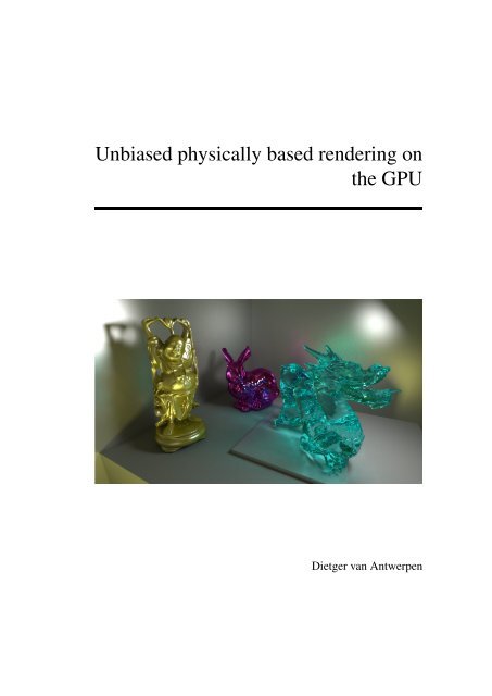
Cover picture: A GPU rendering of the STANFORD scene.
Unbiased physically based rendering on<br />
the GPU<br />
Author: Dietger van Antwerpen<br />
Student id: 1230506<br />
Email: Dietger@xs4all.nl<br />
Abstract<br />
Since the introduction of General-Purpose GPU computing, there has been a significant<br />
increase in ray traversal performance on the GPU. While CPU’s perform reasonably<br />
well on coherent rays with similar origin <strong>and</strong> direction, on current hardware<br />
the GPU vastly outperforms the CPU when it comes to incoherent rays, required for<br />
unbiased rendering. A number of path tracers have been implemented on the GPU,<br />
pulling unbiased physically based rendering to the GPU. However, since the introduction<br />
of the path tracing algorithm, the field of unbiased physically based rendering has<br />
made significant advances. Notorious improvements are BiDirectional Path Tracing<br />
<strong>and</strong> the Metropolis Light Transport algorithm. As of now little effort has been made to<br />
implement these more advanced algorithms on the GPU.<br />
The goal of this thesis is to find efficient GPU implementations for unbiased physically<br />
based rendering methods. The CUDA framework is used for the GPU implementation.<br />
To justify the attempts for moving the sampling algorithm to the GPU, a hybrid<br />
architecture is investigated first, implementing the sampling algorithm on the CPU<br />
while using the GPU as a ray traversal <strong>and</strong> intersection co-processor. Results show<br />
that today’s CPU’s are not well suited for this architecture, making the CPU memory<br />
b<strong>and</strong>width a large bottleneck.<br />
We therefore propose three streaming GPU-only rendering algorithms: a Path<br />
Tracer (PT), a BiDirectional Path Tracer (BDPT) <strong>and</strong> an Energy Redistribution Path<br />
Tracer (ERPT).<br />
The streaming PT uses compaction to remove all terminated paths from the stream,<br />
leaving a continuous stream of active samples. New paths are regenerated in large<br />
batches at the end of the stream, thereby exploiting primary ray coherence during<br />
traversal.<br />
A streaming BDPT is obtained by using a recursive reformulation of the Multiple<br />
Importance Sampling computations. This requires only storage for a single light <strong>and</strong><br />
eye vertex in memory at any time during sample evaluation, making the method’s
ii<br />
memory-footprint independent of the maximum path length <strong>and</strong> allowing high SIMT<br />
efficiency.<br />
We propose an alternative mutation strategy for the ERPT method, further improving<br />
the convergence of the algorithm. Using this strategy, a GPU implementation of<br />
the ERPT method is presented. By sharing mutation chains between all threads within<br />
a GPU warp, efficiency <strong>and</strong> memory coherence is retained.<br />
Finally, the performance of these methods is evaluated <strong>and</strong> it is shown that the<br />
convergence characteristics of the original methods are preserved in our GPU implementations.<br />
<strong>Thesis</strong> Committee:<br />
Chair: Prof.dr.ir. F.W. JANSEN, Faculty EEMCS, <strong>TU</strong> <strong>Delft</strong><br />
University supervisor: Prof.dr.ir. F.W. JANSEN, Faculty EEMCS, <strong>TU</strong> <strong>Delft</strong><br />
Company supervisor: J. BIKKER, Faculty IGAD, NHTV Breda<br />
Committee Member: Dr. A. IOSUP , Faculty EEMCS, <strong>TU</strong> <strong>Delft</strong><br />
Committee Member: Prof.dr.ir. P. DUTRÉ , Faculty CS, K.U. Leuven<br />
Committee Member: Prof.dr. C. WITTEVEEN , Faculty EEMCS, <strong>TU</strong> <strong>Delft</strong>
Preface<br />
This thesis discusses the work I have done for my master project at the <strong>Delft</strong> University of<br />
Technology. The subject of this thesis has been somewhat of a lifelong obsession of mine.<br />
Triggered by animated feature films such as Pixar’s A Bug’s Life <strong>and</strong> Dreamwork’s Antz<br />
<strong>and</strong> Shrek, I developed a fascination for computer graphics <strong>and</strong> photo realistic rendering<br />
in particular. My early high school attempts at building a photo realistic renderer resulted<br />
in a simplistic <strong>and</strong> terribly slow physically based renderer, taking many hours to produce a<br />
picture of a few spheres <strong>and</strong> boxes. But hé, it worked! Since then, I have come a long way<br />
(<strong>and</strong> so has the computer hardware at my disposal). In this thesis, I present my work on<br />
high performance physically based rendering on the GPU, <strong>and</strong> I am proud to say that render<br />
times have dropped from hours to seconds.<br />
I am grateful to my supervisors, Jacco Bikker <strong>and</strong> Erik Jansen, for giving me the opportunity<br />
to work on this interesting topic <strong>and</strong> providing valuable feedback on my work. I<br />
enjoyed working with Jacco Bikker on the Brigade engine, showing me what it means to<br />
really optimize your code. I also like to thank Erik Jansen for providing me with a followup<br />
project on the topic of this thesis. Special thanks goes to Reinier van Antwerpen for<br />
modeling the GLASS EGG scene, used throughout this thesis. Furthermore, I thank Lianne<br />
van Antwerpen for correcting many grammatical errors in this thesis.<br />
While studying physically based rendering, I came to appreciate the fascinating <strong>and</strong><br />
complex light spectacles that surround us every day. This often resulted in exclamations<br />
of excitement whenever a glass of hot tea produced some interesting caustic on the kitchen<br />
table. I thank my family for patiently enduring this habit of mine. I would like to thank<br />
my parents without whom I would not have come this far. In particular, I thank my father<br />
for letting me in on the secret that is called the c programming language, familiarizing me<br />
with many of its intriguing semantics. My mom I thank for getting me through high school;<br />
without her persistence I would probably never have reached my full potential. Finally, I<br />
would like to thank the reader for taking an interest in my work. I hope this thesis will be<br />
an interesting read <strong>and</strong> spark new ideas <strong>and</strong> fresh thoughts by the reader.<br />
Dietger van Antwerpen<br />
<strong>Delft</strong>, the Netherl<strong>and</strong>s<br />
January 5, 2011<br />
iii
Contents<br />
Preface iii<br />
Contents v<br />
List of Figures ix<br />
List of Tables xiii<br />
1 Introduction 1<br />
1.1 Summary of Contributions . . . . . . . . . . . . . . . . . . . . . . . . . . 3<br />
1.2 <strong>Thesis</strong> Outline . . . . . . . . . . . . . . . . . . . . . . . . . . . . . . . . . 4<br />
I Preliminaries 5<br />
2 Unbiased Rendering 7<br />
2.1 Rendering equation . . . . . . . . . . . . . . . . . . . . . . . . . . . . . . 7<br />
2.2 Singularities . . . . . . . . . . . . . . . . . . . . . . . . . . . . . . . . . . 9<br />
2.3 Unbiased Monte Carlo estimate . . . . . . . . . . . . . . . . . . . . . . . . 10<br />
2.4 Path Tracing . . . . . . . . . . . . . . . . . . . . . . . . . . . . . . . . . . 10<br />
2.5 Importance sampling . . . . . . . . . . . . . . . . . . . . . . . . . . . . . 12<br />
2.6 Multiple Importance Sampling . . . . . . . . . . . . . . . . . . . . . . . . 13<br />
2.7 BiDirectional Path Tracing . . . . . . . . . . . . . . . . . . . . . . . . . . 14<br />
2.8 Metropolis sampling . . . . . . . . . . . . . . . . . . . . . . . . . . . . . 17<br />
2.9 Metropolis Light Transport . . . . . . . . . . . . . . . . . . . . . . . . . . 18<br />
2.10 Energy Redistribution Path Tracing . . . . . . . . . . . . . . . . . . . . . . 22<br />
3 GPGPU 25<br />
3.1 Introduction . . . . . . . . . . . . . . . . . . . . . . . . . . . . . . . . . . 25<br />
3.2 Thread Hierarchy . . . . . . . . . . . . . . . . . . . . . . . . . . . . . . . 25<br />
3.3 Memory Hierarchy . . . . . . . . . . . . . . . . . . . . . . . . . . . . . . 27<br />
v
CONTENTS CONTENTS<br />
vi<br />
3.4 Synchronization <strong>and</strong> Communication . . . . . . . . . . . . . . . . . . . . . 30<br />
3.5 Parallel scan . . . . . . . . . . . . . . . . . . . . . . . . . . . . . . . . . . 30<br />
4 Related Work 33<br />
4.1 GPU ray tracing . . . . . . . . . . . . . . . . . . . . . . . . . . . . . . . . 33<br />
4.2 Unbiased rendering . . . . . . . . . . . . . . . . . . . . . . . . . . . . . . 35<br />
II GPU Tracers 37<br />
5 The Problem Statement 39<br />
5.1 Related work . . . . . . . . . . . . . . . . . . . . . . . . . . . . . . . . . 40<br />
5.2 Context . . . . . . . . . . . . . . . . . . . . . . . . . . . . . . . . . . . . 42<br />
6 Hybrid Tracer 43<br />
6.1 Introduction . . . . . . . . . . . . . . . . . . . . . . . . . . . . . . . . . . 43<br />
6.2 Hybrid architecture . . . . . . . . . . . . . . . . . . . . . . . . . . . . . . 43<br />
6.3 Results . . . . . . . . . . . . . . . . . . . . . . . . . . . . . . . . . . . . . 46<br />
7 Path Tracer (PT) 51<br />
7.1 Introduction . . . . . . . . . . . . . . . . . . . . . . . . . . . . . . . . . . 51<br />
7.2 Two-Phase PT . . . . . . . . . . . . . . . . . . . . . . . . . . . . . . . . . 51<br />
7.3 GPU PT . . . . . . . . . . . . . . . . . . . . . . . . . . . . . . . . . . . . 53<br />
7.4 Stream compaction . . . . . . . . . . . . . . . . . . . . . . . . . . . . . . 54<br />
7.5 Results . . . . . . . . . . . . . . . . . . . . . . . . . . . . . . . . . . . . . 58<br />
8 Streaming BiDirectional Path Tracer (SBDPT) 67<br />
8.1 Introduction . . . . . . . . . . . . . . . . . . . . . . . . . . . . . . . . . . 67<br />
8.2 Recursive Multiple Importance Sampling . . . . . . . . . . . . . . . . . . 69<br />
8.3 SBDPT . . . . . . . . . . . . . . . . . . . . . . . . . . . . . . . . . . . . 77<br />
8.4 GPU SBDPT . . . . . . . . . . . . . . . . . . . . . . . . . . . . . . . . . 80<br />
9 Energy Redistribution Path Tracer (ERPT) 93<br />
9.1 Introduction . . . . . . . . . . . . . . . . . . . . . . . . . . . . . . . . . . 93<br />
9.2 ERPT mutation . . . . . . . . . . . . . . . . . . . . . . . . . . . . . . . . 93<br />
9.3 GPU ERPT . . . . . . . . . . . . . . . . . . . . . . . . . . . . . . . . . . 103<br />
III Results 121<br />
10 Comparison 123<br />
10.1 Performance . . . . . . . . . . . . . . . . . . . . . . . . . . . . . . . . . . 123<br />
10.2 Convergence . . . . . . . . . . . . . . . . . . . . . . . . . . . . . . . . . 126<br />
11 Conclusions <strong>and</strong> Future Work 129
CONTENTS CONTENTS<br />
Bibliography 131<br />
A Glossary 137<br />
B Sample probability 139<br />
B.1 Vertex sampling . . . . . . . . . . . . . . . . . . . . . . . . . . . . . . . . 140<br />
B.2 Subpath sampling . . . . . . . . . . . . . . . . . . . . . . . . . . . . . . . 141<br />
B.3 Bidirectional sampling . . . . . . . . . . . . . . . . . . . . . . . . . . . . 141<br />
C Camera Model 143<br />
D PT Algorithm 145<br />
D.1 Path contribution . . . . . . . . . . . . . . . . . . . . . . . . . . . . . . . 145<br />
D.2 MIS weights . . . . . . . . . . . . . . . . . . . . . . . . . . . . . . . . . . 146<br />
D.3 Algorithm . . . . . . . . . . . . . . . . . . . . . . . . . . . . . . . . . . . 147<br />
E BDPT Algorithm 149<br />
E.1 Path contribution . . . . . . . . . . . . . . . . . . . . . . . . . . . . . . . 149<br />
E.2 Algorithm . . . . . . . . . . . . . . . . . . . . . . . . . . . . . . . . . . . 151<br />
F MLT Mutations 155<br />
F.1 Acceptance probability . . . . . . . . . . . . . . . . . . . . . . . . . . . . 155<br />
F.2 Algorithm . . . . . . . . . . . . . . . . . . . . . . . . . . . . . . . . . . . 158<br />
vii
List of Figures<br />
1.1 Approximation vs physically based rendering . . . . . . . . . . . . . . . . . . 2<br />
2.1 Light transport geometry . . . . . . . . . . . . . . . . . . . . . . . . . . . . . 7<br />
2.2 Measurement contribution function . . . . . . . . . . . . . . . . . . . . . . . . 9<br />
2.3 PT sample . . . . . . . . . . . . . . . . . . . . . . . . . . . . . . . . . . . . . 11<br />
2.4 Importance Sampling . . . . . . . . . . . . . . . . . . . . . . . . . . . . . . . 13<br />
2.5 BDPT Sample . . . . . . . . . . . . . . . . . . . . . . . . . . . . . . . . . . . 15<br />
2.6 Lens mutation . . . . . . . . . . . . . . . . . . . . . . . . . . . . . . . . . . . 20<br />
2.7 Lai Lens mutation . . . . . . . . . . . . . . . . . . . . . . . . . . . . . . . . . 21<br />
2.8 Caustic mutation . . . . . . . . . . . . . . . . . . . . . . . . . . . . . . . . . 21<br />
3.1 CUDA thread hierarchy . . . . . . . . . . . . . . . . . . . . . . . . . . . . . . 26<br />
3.2 CUDA device architecture . . . . . . . . . . . . . . . . . . . . . . . . . . . . 28<br />
3.3 Coalesced memory access with compute capability 1.0 or 1.1 . . . . . . . . . . 28<br />
3.4 Coalesced memory access with compute capability 1.2 . . . . . . . . . . . . . 29<br />
5.1 Test scenes . . . . . . . . . . . . . . . . . . . . . . . . . . . . . . . . . . . . 41<br />
6.1 Sampler flowchart . . . . . . . . . . . . . . . . . . . . . . . . . . . . . . . . . 44<br />
6.2 CPU-GPU pipeline . . . . . . . . . . . . . . . . . . . . . . . . . . . . . . . . 45<br />
6.3 CPU PT performance . . . . . . . . . . . . . . . . . . . . . . . . . . . . . . . 46<br />
6.4 Hybrid PT performance . . . . . . . . . . . . . . . . . . . . . . . . . . . . . . 47<br />
6.5 Hybrid PT performance partition . . . . . . . . . . . . . . . . . . . . . . . . . 48<br />
6.6 Hybrid Sibenik cathedral rendering . . . . . . . . . . . . . . . . . . . . . . . . 49<br />
7.1 Two-Phase PT flowchart . . . . . . . . . . . . . . . . . . . . . . . . . . . . . 52<br />
7.2 Rearanging rays for immediate coalesced packing . . . . . . . . . . . . . . . . 56<br />
7.3 Sampler Stream PT Flowchart . . . . . . . . . . . . . . . . . . . . . . . . . . 57<br />
7.4 SSPT streams . . . . . . . . . . . . . . . . . . . . . . . . . . . . . . . . . . . 58<br />
7.5 GPU PT performance . . . . . . . . . . . . . . . . . . . . . . . . . . . . . . . 61<br />
7.6 PT Extension ray traversal performance . . . . . . . . . . . . . . . . . . . . . 62<br />
ix
List of Figures List of Figures<br />
x<br />
7.7 TPPT time partition . . . . . . . . . . . . . . . . . . . . . . . . . . . . . . . . 62<br />
7.8 SSPT time partition . . . . . . . . . . . . . . . . . . . . . . . . . . . . . . . . 63<br />
7.9 TPPT performance vs. stream size . . . . . . . . . . . . . . . . . . . . . . . . 64<br />
7.10 SSPT performance vs. stream size . . . . . . . . . . . . . . . . . . . . . . . . 64<br />
7.11 GPU PT conference room rendering . . . . . . . . . . . . . . . . . . . . . . . 65<br />
8.1 MIS denominator . . . . . . . . . . . . . . . . . . . . . . . . . . . . . . . . . 70<br />
8.2 SBDPT sample . . . . . . . . . . . . . . . . . . . . . . . . . . . . . . . . . . 77<br />
8.3 SBDPT flowchart . . . . . . . . . . . . . . . . . . . . . . . . . . . . . . . . . 81<br />
8.4 Collapsed SBDPT flowchart . . . . . . . . . . . . . . . . . . . . . . . . . . . 82<br />
8.5 SBDPT vertex memory access . . . . . . . . . . . . . . . . . . . . . . . . . . 83<br />
8.6 SBDPT performance with stream compaction . . . . . . . . . . . . . . . . . . 88<br />
8.7 SBDPT time partition . . . . . . . . . . . . . . . . . . . . . . . . . . . . . . . 88<br />
8.8 SSPT vs SBDPT . . . . . . . . . . . . . . . . . . . . . . . . . . . . . . . . . 90<br />
8.9 Contribution of bidirectional strategies . . . . . . . . . . . . . . . . . . . . . . 91<br />
9.1 Feature shapes . . . . . . . . . . . . . . . . . . . . . . . . . . . . . . . . . . . 97<br />
9.2 High correlation in feature . . . . . . . . . . . . . . . . . . . . . . . . . . . . 98<br />
9.3 Local feature optimum . . . . . . . . . . . . . . . . . . . . . . . . . . . . . . 99<br />
9.4 Low energy feature . . . . . . . . . . . . . . . . . . . . . . . . . . . . . . . . 99<br />
9.5 Improved mutation strategy . . . . . . . . . . . . . . . . . . . . . . . . . . . . 102<br />
9.6 ERPT flowchart . . . . . . . . . . . . . . . . . . . . . . . . . . . . . . . . . . 105<br />
9.7 ERPT path vertex access . . . . . . . . . . . . . . . . . . . . . . . . . . . . . 108<br />
9.8 ERPT progress estimation . . . . . . . . . . . . . . . . . . . . . . . . . . . . 112<br />
9.9 ERPT performance . . . . . . . . . . . . . . . . . . . . . . . . . . . . . . . . 115<br />
9.10 ERPT time partition . . . . . . . . . . . . . . . . . . . . . . . . . . . . . . . . 116<br />
9.11 Complex caustic with ERPT <strong>and</strong> SBDPT . . . . . . . . . . . . . . . . . . . . 117<br />
9.12 ERPT <strong>and</strong> SSPT comparison . . . . . . . . . . . . . . . . . . . . . . . . . . . 118<br />
9.13 Invisible date with ERPT, SBDPT <strong>and</strong> SSPT . . . . . . . . . . . . . . . . . . . 119<br />
9.14 Stanford scene with ERPT <strong>and</strong> SBDPT . . . . . . . . . . . . . . . . . . . . . . 120<br />
10.1 Iteration performance comparison . . . . . . . . . . . . . . . . . . . . . . . . 124<br />
10.2 Traversal performance comparison . . . . . . . . . . . . . . . . . . . . . . . . 125<br />
10.3 Sponza with ERPT, SBDPT <strong>and</strong> SSPT . . . . . . . . . . . . . . . . . . . . . . 126<br />
10.4 Glass Egg with ERPT, SBDPT <strong>and</strong> SSPT . . . . . . . . . . . . . . . . . . . . 127<br />
10.5 Invisible Date with ERPT, SBDPT <strong>and</strong> SSPT . . . . . . . . . . . . . . . . . . 128<br />
B.1 Conversion between unit projected solid angle <strong>and</strong> unit area . . . . . . . . . . . 139<br />
B.2 Vertex sampling . . . . . . . . . . . . . . . . . . . . . . . . . . . . . . . . . . 140<br />
B.3 Bidirectional Sampled Path . . . . . . . . . . . . . . . . . . . . . . . . . . . . 142<br />
C.1 Camera model . . . . . . . . . . . . . . . . . . . . . . . . . . . . . . . . . . . 144<br />
D.1 Implicit path contribution . . . . . . . . . . . . . . . . . . . . . . . . . . . . . 146<br />
D.2 Explicit path contribution . . . . . . . . . . . . . . . . . . . . . . . . . . . . . 146
List of Figures List of Figures<br />
E.1 One eye subpath contribution . . . . . . . . . . . . . . . . . . . . . . . . . . . 151<br />
E.2 Bidirectional path contribition . . . . . . . . . . . . . . . . . . . . . . . . . . 151<br />
F.1 Acceptance probability for partial lens mutation . . . . . . . . . . . . . . . . . 157<br />
F.2 Acceptance probability for full lens mutation . . . . . . . . . . . . . . . . . . 157<br />
F.3 Acceptance probability for partial caustic mutation . . . . . . . . . . . . . . . 157<br />
F.4 Acceptance probability for full caustic mutation . . . . . . . . . . . . . . . . . 158<br />
xi
List of Tables<br />
5.1 Test scenes . . . . . . . . . . . . . . . . . . . . . . . . . . . . . . . . . . . . 42<br />
7.1 TPPT SIMT efficiency . . . . . . . . . . . . . . . . . . . . . . . . . . . . . . 59<br />
7.2 SSPT SIMT efficiency . . . . . . . . . . . . . . . . . . . . . . . . . . . . . . 60<br />
7.3 GPU PT memory usage . . . . . . . . . . . . . . . . . . . . . . . . . . . . . . 63<br />
8.1 SBDPT SIMT efficiency . . . . . . . . . . . . . . . . . . . . . . . . . . . . . 87<br />
8.2 SBDPT memory usage . . . . . . . . . . . . . . . . . . . . . . . . . . . . . . 89<br />
9.1 Average rays per mutation . . . . . . . . . . . . . . . . . . . . . . . . . . . . 113<br />
9.2 Average mutation acceptance probability . . . . . . . . . . . . . . . . . . . . . 113<br />
9.3 ERPT path tracing SIMT efficiency . . . . . . . . . . . . . . . . . . . . . . . 114<br />
9.4 ERPT energy redistribution SIMT efficiency . . . . . . . . . . . . . . . . . . . 114<br />
9.5 ERPT memory usage . . . . . . . . . . . . . . . . . . . . . . . . . . . . . . . 116<br />
xiii
List of Algorithms<br />
1 Metropolis Light Transport . . . . . . . . . . . . . . . . . . . . . . . . . . 19<br />
2 Energy Redistribution . . . . . . . . . . . . . . . . . . . . . . . . . . . . . 23<br />
3 Parallel Scan . . . . . . . . . . . . . . . . . . . . . . . . . . . . . . . . . 31<br />
4 Mutate . . . . . . . . . . . . . . . . . . . . . . . . . . . . . . . . . . . . . 106<br />
5 PT . . . . . . . . . . . . . . . . . . . . . . . . . . . . . . . . . . . . . . . 148<br />
6 SampleEyePath . . . . . . . . . . . . . . . . . . . . . . . . . . . . . . . . 152<br />
7 SampleLightPath . . . . . . . . . . . . . . . . . . . . . . . . . . . . . . . 153<br />
8 Connect . . . . . . . . . . . . . . . . . . . . . . . . . . . . . . . . . . . . 154<br />
9 CausticMutation . . . . . . . . . . . . . . . . . . . . . . . . . . . . . . . . 159<br />
10 LensMutation . . . . . . . . . . . . . . . . . . . . . . . . . . . . . . . . . 160<br />
xv
Chapter 1<br />
Introduction<br />
Since the introduction of computer graphics, synthesizing computer images has found many<br />
useful applications. Of these, the best known are probably those in the entertainment industries,<br />
where image synthesis is used to create visually compelling computer games <strong>and</strong> to<br />
add special effects to movies. Besides these <strong>and</strong> many others, important applications are<br />
found in advertisement, medicine, architecture <strong>and</strong> product design. In many of these applications,<br />
image synthesis is used to give a realistic impression of the illumination in virtual<br />
3D scenes. For example, in architecture, CG is used to answer questions about the illumination<br />
in a designed building [15]. Such information is used to evaluate the design before<br />
realizing the building. In advertising <strong>and</strong> film production, computer graphics is used to<br />
combine virtual 3D models with video recordings to visualize scenes that would otherwise<br />
be impossible or prohibitively expensive to capture on film. Both these applications require<br />
a high level of realism, giving an accurate prediction of the appearance of the scene <strong>and</strong><br />
making the synthesized images indistinguishable from real photos of similar scenes in the<br />
real world.<br />
Physically based rendering algorithms use mathematical models of physical light transport<br />
for image synthesis <strong>and</strong> are capable of accurately rendering such realistic images. For<br />
most practical applications, physically based rendering algorithms require a lot of computational<br />
power to produce an accurate result. Therefore, these algorithms are mostly used<br />
for off-line rendering, often on large computer clusters. This lack of immediate feedback<br />
complicates the work for the designer of virtual environments.<br />
To get some immediate feedback, the designer usually resorts to approximate solutions<br />
[6, 32, 36, 55]. Although interactive, these approximations sacrifice accuracy for performance.<br />
Complex illumination effects such as indirect light <strong>and</strong> caustics are roughly approximated<br />
or completely absent in the approximation. Figure 1.1 shows the difference between<br />
an approximation 1 <strong>and</strong> a physically based rendering. Although the approximation looks<br />
plausible, it is far from physically accurate. The lack of accuracy reduces its usefulness to<br />
the designer. Designers would benefit greatly from interactive or near-interactive physically<br />
based rendering algorithms on a single workstation for fast <strong>and</strong> accurate feedback on their<br />
1 This approximation algorithm simulates a single light indirection <strong>and</strong> supports only perfect specular <strong>and</strong><br />
perfect diffuse materials.<br />
1
2<br />
(a) (b)<br />
Introduction<br />
Figure 1.1: Rendering of the GLASS EGG scene with (a) an approximation algorithm <strong>and</strong><br />
(b) a physically based algorithm.<br />
designs.<br />
The speed of physically based rendering can be improved by either using more advanced<br />
algorithms, or by optimizing the implementation of these algorithms. Since the advent of<br />
physically based rendering, several advanced physically based rendering algorithms, capable<br />
of rendering very complex scenes, have been developed <strong>and</strong> implemented on the CPU.<br />
At the same time, many fast approximation algorithms have been developed for the GPU.<br />
Because these algorithms are used by most modeling software packages, modeling workstations<br />
usually contain one or more powerful GPUs. Nowadays, these GPUs often provide<br />
more raw processing power <strong>and</strong> memory b<strong>and</strong>width than the workstations main processor<br />
<strong>and</strong> system memory [13]. Therefore, the performance of a physically based rendering<br />
algorithm could benefit greatly from utilizing the available GPUs.<br />
The goal of this thesis will be to find efficient GPU implementations for physically<br />
based rendering algorithms. Parts of these algorithms, such as ray-scene intersection tests,<br />
have already been efficiently implemented on the GPU, significantly outperforming similar<br />
CPU implementations. Furthermore, some simple rendering algorithms have been fully<br />
implemented on the GPU. However, little effort has been made to implement more advanced<br />
physically based rendering algorithms on the GPU. Implementing these algorithms on the<br />
GPU will allow for a wider range of scenes to be rendered accurately <strong>and</strong> at high speed<br />
on a single workstation. In the following sections, we will give a brief summary of our<br />
contributions <strong>and</strong> give a short overview of the thesis outline.
Introduction 1.1 Summary of Contributions<br />
1.1 Summary of Contributions<br />
In this thesis we will present the following contributions:<br />
• We present a general framework for hybrid physically based rendering algorithms<br />
where ray traversal is performed on the GPU while shading <strong>and</strong> ray generation are<br />
performed on the CPU.<br />
• We show that on modern workstations the performance of a hybrid architecture is<br />
limited by the memory b<strong>and</strong>width of system memory. This reduces scalability <strong>and</strong><br />
prevents the full utilization of the GPU, justifying our further attempts to fully implement<br />
the rendering algorithms on the GPU.<br />
• We present an alternative method for computing Multiple Importance Sampling weights<br />
for BDPT. By recursively computing two extra quantities during sample construction,<br />
we show that the weights can be computed using a fixed amount of computations <strong>and</strong><br />
data per connection, independent of the sample path lengths. This allows for efficient<br />
data parallel weight computation on the GPU.<br />
• We introduce the notion of mutation features <strong>and</strong> use these to investigate the noise<br />
occurring in ERPT. We show that structural noise patterns in ERPT can be understood<br />
in the context of mutation features.<br />
• We propose an alternative mutation strategy for the ERPT method. We show that<br />
by increasing mutation feature size, our mutation strategy trades structural noise for<br />
more uniform noise. This allows for longer mutation chains, required for an efficient<br />
GPU implementation.<br />
• We present streaming GPU implementations of three well known, physically based<br />
rendering algorithms: Path Tracing (PT), BiDirectional Path Tracing (BDPT) <strong>and</strong> Energy<br />
Redistribution Path Tracing (ERPT). We show how our implementations achieve<br />
high degrees of coarse grained <strong>and</strong> fine grained parallelism, required to fully utilize<br />
the GPU. Furthermore, we discuss how memory access patterns are adapted to allow<br />
for high effective memory b<strong>and</strong>width on the GPU.<br />
– We show how to increase the ray traversal performance of GPU samplers by<br />
immediately packing output rays in a compact output stream.<br />
– Furthermore, we show that immediate sampler stream compaction can be used<br />
to speed up PT <strong>and</strong> increase ray traversal performance further by exploiting<br />
primary ray coherence.<br />
– We present a streaming adaption of the BDPT algorithm, called SBDPT. We<br />
show how our recursive computation of MIS weights allows us to only store<br />
a single light <strong>and</strong> eye vertex in memory at any time during sample evaluation,<br />
making the methods memory footprint independent of the path length <strong>and</strong> allowing<br />
for high GPU efficiency.<br />
3
1.2 <strong>Thesis</strong> Outline Introduction<br />
4<br />
– By generating mutation chains in batches of 32, our ERPT implementation realizes<br />
high GPU efficiency <strong>and</strong> effective memory b<strong>and</strong>width. All mutation chains<br />
in a batch follow the same code path, resulting in high fine grained parallelism.<br />
• We compare the three implementations in terms of performance <strong>and</strong> convergence<br />
speed. We show that the convergence characteristics of the three rendering algorithms<br />
are preserved in our adapted GPU implementations. Furthermore, we show that the<br />
performance of the algorithms are all in the same order of magnitude.<br />
1.2 <strong>Thesis</strong> Outline<br />
The thesis is divided in three parts. Part I contains background information on the subject<br />
of unbiased rendering <strong>and</strong> GPGPU programming. In chapter 2, we will give a short introduction<br />
to physically based rendering. In this discussion, we will emphasize the use of<br />
importance sampling to improve physically based rendering algorithms <strong>and</strong> show how this<br />
naturally leads to the three well known rendering algorithms PT, BDPT <strong>and</strong> ERPT. This<br />
chapter will introduce all related notation <strong>and</strong> terminology we will be using in the rest of<br />
this thesis. Next, in chapter 3, we give an overview of the General Purpose GPU architecture<br />
in the context of CUDA: the parallel computing architecture developed by NVIDIA<br />
[13]. In our discussion we will focus mainly on how to achieve high parallelism <strong>and</strong> memory<br />
b<strong>and</strong>width, which translates to high overall performance. Finally, we will discuss the<br />
parallel scan primitive. In chapter 4 we discuss related work on ray tracing <strong>and</strong> unbiased<br />
rendering using the GPU. We will further discuss some variations on the unbiased rendering<br />
algorithms not mentioned in chapter 2.<br />
In part II we present the main contributions of this thesis. We start with a problem<br />
statement in chapter 5. In chapter 6, we investigate a hybrid architecture where the rendering<br />
algorithm is implemented on the CPU, using the GPU for ray traversal <strong>and</strong> intersection<br />
only. We will show that the CPU side easily becomes the bottleneck, limiting the performance<br />
gained by using a GPU. Following, in chapter 7, we present our GPU Path Tracer.<br />
First, we present the Two-Phase PT implementation which forms a starting point for the<br />
BDPT <strong>and</strong> EPRT implementations in later chapters. We will further show how to improve<br />
the performance of this PT through stream compaction, resulting in a highly optimized implementation.<br />
After that, we present our SBDPT algorithm in chapter 8. We first present<br />
a recursive formulation for Multiple Importance Sampling <strong>and</strong> show how this formulation<br />
is used in the SBDPT algorithm, allowing for an efficient GPU implementation. Finally, in<br />
chapter 9, we study the characteristics of the ERPT mutation strategy using the concept of<br />
mutation features. We will then propose an improved mutation strategy, which we use in<br />
our ERPT implementation. Next, we present our streaming ERPT algorithm <strong>and</strong> its GPU<br />
implementation.<br />
Finally, in part III, we discuss our findings. We first compare the performance <strong>and</strong><br />
convergence characteristics of the three GPU implementations in chapter 10. We conclude<br />
this thesis in chapter 11, with a discussion <strong>and</strong> some ideas for future work.<br />
Lastly, the appendix provides a small glossary of frequently used terms <strong>and</strong> abbreviations<br />
<strong>and</strong> further details on the PT, BDPT <strong>and</strong> ERPT algorithms.
Part I<br />
Preliminaries<br />
5
Chapter 2<br />
Unbiased Rendering<br />
In this chapter, we will give a short introduction to physically based rendering. In this discussion,<br />
we will emphasize the use of importance sampling to improve physically based<br />
rendering algorithms <strong>and</strong> show how this naturely leads to the three well known rendering<br />
algorithms: Path Tracing, BiDirectional Path Tracing <strong>and</strong> Energy Redistribution Path Tracing.<br />
This chapter will also introduce all related notation <strong>and</strong> terminology we will be using in<br />
the rest of this thesis. For a more thorough discussion on most of the topics encountered in<br />
this chapter, we redirect the reader to [16]. For an extensive compendium of useful formulas<br />
<strong>and</strong> equations related to unbiased physically based rendering. we refer to [17, 2].<br />
2.1 Rendering equation<br />
x''<br />
Figure 2.1: Geometry for the light transport equation.<br />
Physical based light transport in free space (vacuum) is modeled by the light transport<br />
equation. This equation describes how radiance arriving at surface point x ′′ from surface<br />
point x ′ relates to radiance arriving at x ′ (figure 2.1). Because light transport is usually<br />
perceived in equilibrium, the equation describes the equilibrium state:<br />
L x ′ → x ′′ ′ ′′<br />
= Le x → x <br />
+ L<br />
M<br />
x → x ′ ′ ′′<br />
fs x → x → x G x ↔ x ′ dAM (x) (2.1)<br />
x'<br />
x<br />
7
2.1 Rendering equation Unbiased Rendering<br />
8<br />
In this equation, L(x ′ → x ′′ ) is the radiance arriving at surface point x ′′ from surface point<br />
x ′ due to all incoming radiance at x ′ from all surface points M. M is the union of all scene<br />
surfaces. Le (x ′ → x ′′ ) is the radiance emitted from x ′ arriving at x ′′ . fs (x → x ′ → x ′′ ) is<br />
the Bidirectional Scattering Distribution Function (BSDF), used to model the local surface<br />
material. It describes the fraction of radiance arriving at x ′ from x that is scattered towards<br />
x ′′ . Finally, G(x ↔ x ′ ) is the geometric term to convert from unit projected solid angle to<br />
unit surface area.<br />
G x ↔ x ′ = V x ↔ x ′ |cos(θo)cos(θ ′ i )|<br />
||x − x ′ || 2<br />
(2.2)<br />
In this term, V (x ↔ x ′ ) is the visibility term, which is 1 iff the two surface points are visible<br />
from one another <strong>and</strong> 0 otherwise. θ ′ i <strong>and</strong> θo are the angles between the local surface normals<br />
<strong>and</strong> respectively the incoming <strong>and</strong> outgoing light flow.<br />
The light transport equation is usually expressed as an integral over unit projected solid<br />
angles instead of surface area, by omitting the geometric factor <strong>and</strong> integrating over the<br />
projected unit hemisphere. We will however only concern ourselves with the surface area<br />
formulation.<br />
In the context of rendering, the transport equation is often called the rendering equation.<br />
When rendering an image, each image pixel j is modeled as a radiance sensor. Each sensor<br />
measures radiance over surface area <strong>and</strong> has a sensor sensitivity function Wj(x → x ′ ), describing<br />
the sensor’s sensitivity to radiance arriving at x ′ from x. Let I be the surface area<br />
of the image plane, then the measurement equation for pixel j equals:<br />
<br />
′<br />
Ij = Wj x → x<br />
I×M<br />
L x → x ′ G x ↔ x ′ ′<br />
dAI x dAM (x) (2.3)<br />
In this thesis, we used a sensor sensitivity function corresponding to a simple finite aperture<br />
camera model. For more details on the finite aperture camera model, see appendix C.<br />
Note that the expression for radiance L is recursive. Each recursion represents the scattering<br />
of light at a surface point. A sequence of scattering events represents a light transport<br />
path from a light source to the pixel sensor. The measured radiance leaving a light source<br />
<strong>and</strong> arriving at the image plane along some light transport path x0...xk ∈ I × M k , can be<br />
expressed as:<br />
f j(x0 ···xk) =Le (xk → xk−1)G(xk → xk−1)<br />
k−1<br />
∏ fs (xi+1 → xi → xi−1)G(xi ↔ xi−1)·<br />
i=1<br />
Wj (x1 → x0)<br />
(2.4)<br />
This function is called the measurement contribution function. The surface points x0 ···xk<br />
are called the path vertices <strong>and</strong> form a light transport path X of length k (see figure 2.2).<br />
Note that the vertices on the path are arranged in reverse order, with x0 on the image plane<br />
<strong>and</strong> xk on the light source. This is because constructing a path in reverse order, from eye<br />
to light source, is often more convenient. The recursion in the measurement equation is
Unbiased Rendering 2.2 Singularities<br />
Figure 2.2: Measurement contribution function for an example path.<br />
removed by exp<strong>and</strong>ing the equation to<br />
Ij =<br />
∞ <br />
∑<br />
k=1 I×Mk f j (x0 ···xk)dAI(x0)dAM(x1)···dAM(xk) (2.5)<br />
The set of all light transport paths of length k is defined as Ωk = I × M k . This gives<br />
rise to a unified path space, defined as Ω = ∞ i=1 Ωi <strong>and</strong> a corresponding product measure<br />
dΩ(Xk) = dAI (x0) × dAM (x1) × ··· × dAM (xk) on path space. The measurement integral<br />
can be expressed as an integral of the measurement contribution function over this unified<br />
path space, resulting in<br />
Ij =<br />
<br />
f j(X)dΩ(X)<br />
Ω<br />
(2.6)<br />
In this equation, the measurement contribution function f j describes the amount of energy<br />
per unit path space as measured by sensor j. Physical based rendering concerns itself with<br />
estimating this equation for all image pixels.<br />
2.2 Singularities<br />
Many of the aforementioned functions may contain singularities. For example, the BSDF of<br />
perfect reflective <strong>and</strong> refractive materials is modeled using Dirac functions. Furthermore,<br />
Le may exhibit singularities to model purely directional light sources. Finally, common<br />
camera models such as the pinhole camera are modeled using Dirac functions in the sensor<br />
sensitivity functions Wj. Special care must be taken to support these singularities. In this<br />
work, we assume that the camera model contains a singularity <strong>and</strong> that BSDF’s may exhibit<br />
singularities. However, unless explicitly addressed, we assume that light sources do not<br />
exhibit singularities.<br />
Heckbert introduced a notation to classify light transport paths using regular expressions<br />
of the form E (S|D) ∗ L [24]. Each symbol represents a path vertex. E represents the eye <strong>and</strong><br />
is the first path vertex. This vertex is followed by any number of path vertices, classified<br />
as specular(S) or diffuse(D) vertices. A path vertex is said to be specular whenever the<br />
9
2.3 Unbiased Monte Carlo estimate Unbiased Rendering<br />
10<br />
scattering event follows a singularity in the local BSDF, also called a specular bounce.<br />
Finally, the last vertex is classified as a light source(L). We refer to the classification of a<br />
path as its signature.<br />
2.3 Unbiased Monte Carlo estimate<br />
The measurement equation contains an integral of a possibly non-continuous function over<br />
the multidimensional path space. Therefore, the measurement equation is usually estimated<br />
using the Monte Carlo method. The Monte Carlo method uses r<strong>and</strong>om sampling to estimate<br />
an integral. The idea is to sample N points X1 ···XN according to some convenient<br />
probability density function p : Ω → R. Then, the integral I = <br />
Ω f (x)µ(x) is estimated as<br />
follows<br />
I = E [FN] ≈ FN = 1<br />
N<br />
N f (Xi)<br />
∑<br />
i=1 p(Xi)<br />
(2.7)<br />
This estimator FN is called unbiased because its expected value E [FN] equals the desired<br />
outcome I, independent of the number of samples N. Note that a biased estimator may still<br />
be consistent if it satisfies limN→∞ FN = I, that is, the bias goes to zero as the number of<br />
samples goes to infinity.<br />
In the context of rendering, the N samples used in the estimate are r<strong>and</strong>om light transport<br />
paths from unified path space. These paths are generated by a sampler. Possible samplers<br />
are the Path Tracing sampler(PT), BiDirectional Path Tracing sampler(BDPT) or Energy<br />
Redistribution Path Tracing(ERPT) sampler, discussed in later sections. The different samplers<br />
generate paths according to different probability distributions.<br />
Generating a path is usually computationally expensive because it requires the tracing<br />
of multiple rays through the scene. Although a sampler may generate one independent path<br />
at a time, it is often computationally beneficial to generate collections of correlated paths.<br />
From now on, when referring to a sample generated by some sampler, we mean such a<br />
collection of paths generated by the sampler. When generating collections of paths, special<br />
care must be taken to compute the probability with which each path is generated by the<br />
sampler. A simple solution is to partition path space, allowing a sampler to generate at<br />
most one path per part within each sample; for example by using the partition Ω = ∞ i=1 Ωi<br />
<strong>and</strong> allowing at most one path per collection for each path length. This often simplifies<br />
computations considerably. In the next section, this method is used in the PT sampler.<br />
2.4 Path Tracing<br />
In path tracing, a collection of paths is sampled backward, starting at the eye. Figure 2.3<br />
shows a single path tracing sample. A sampler starts by tracing a path y0 ···yk backwards<br />
from the eye, through the image plane into the scene. The path is repeatedly extended with<br />
another path vertex until it is terminated. At each path vertex, the path is terminated with a<br />
certain probability using Russian roulette. Each path vertex yi is explicitly connected to a<br />
r<strong>and</strong>om point z on a light source to form the complete light transport path y0 ···yiz from the
Unbiased Rendering 2.4 Path Tracing<br />
Y 0<br />
Y 1<br />
Y 2<br />
Figure 2.3: Path tracing sample.<br />
eye to the light source. These complete paths are called explicit paths. However, when the<br />
path ’accidentally’ hits a light source at vertex yk, this path y0 ···yk also forms a valid light<br />
transport path. Such paths are called implicit paths. Hence, light transport paths may be<br />
generated as either an explicit or implicit path. For simplicity, we assume that light sources<br />
do not reflect any light, so the path may be terminated whenever it hits a light source.<br />
A path vertex must be diffuse for an explicit connection to make sense, because otherwise<br />
the BSDF will be non-zero with zero probability. Therefore, path space is partitioned<br />
in explicit <strong>and</strong> implicit paths, where explicit paths must be of the form E (S|D) ∗ DL while<br />
implicit paths must be of the form E L|(S|D) ∗ SL . All other explicit <strong>and</strong> implicit paths are<br />
discarded. Note that a PT sample contains at most one explicit <strong>and</strong> one implicit path for<br />
each path length. Hence, by further partitioning path space according to path length, it is<br />
guaranteed that the sampler generates at most one valid light transport path per part.<br />
When the PT sampler extends the partial path y0 ···yi with another vertex yi+1, an outgoing<br />
direction Ψi at yi is sampled per projected solid angle <strong>and</strong> the corresponding ray is<br />
intersected with the scene to find the next path vertex yi+1. Hence, path vertices are sampled<br />
per projected solid angle. To compute the sampling probability per unit area, the probability<br />
is converted using the geometric term:<br />
PA (yi → yi+1) = P σ ⊥ (yi → yi+1)G(yi ↔ yi+1) (2.8)<br />
For more details on converting probabilities per unit projected solid angle to probabilities<br />
per unit area <strong>and</strong> back, see appendix B. Note that in practice, P σ ⊥ (yi → yi+1) usually<br />
also depends on the incoming direction. To emphasize this, one could instead write<br />
P σ ⊥ (yi−1 → yi → yi+1). To keep things simple, we omitted this. It is however important<br />
to keep in mind that the incoming direction is usually needed to calculate this probability.<br />
We further assume that the inverse termination probability for Russian roulette is incorporated<br />
in the probability PA (yi → yi+1) of sampling yi+1. Because the point z on the light<br />
source <strong>and</strong> y0 on the eye are directly sampled per unit area, no further probability conversions<br />
are required for these vertices. The probability that a sampler generates some explicit,<br />
Z<br />
Y 3<br />
Z<br />
11
2.5 Importance sampling Unbiased Rendering<br />
12<br />
respectively implicit, path as part of a PT sample equals<br />
i−1<br />
P(y0 ···yiz) = PA (y0) ∏ PA (y j → y j+1)PA (z)<br />
j=0<br />
k−1<br />
P(y0 ···yk) = PA (y0) ∏ PA (yi → yi+1)<br />
i=0<br />
For more details on generating <strong>and</strong> evaluating path tracing samples, see appendix D.<br />
2.5 Importance sampling<br />
(2.9)<br />
A sampler may sample light transport paths according to any convenient probability density<br />
f (X)<br />
function p, provided that p(X) is finite whenever f (X) > 0. However, the probability density<br />
function greatly influences the quality of the estimator. A good measure for quality is the<br />
variance of an estimator, where smaller variance results in a better estimator. To reduce<br />
variance in the estimator, p should resemble f as much as possible. To see why this is true,<br />
f (X)<br />
assume that p equals f up to some normalization constant c, so that p(X) = c for all X ∈ Ω.<br />
Then the estimator reduces to<br />
<br />
f (X1)<br />
F1 = E = E [c] = c (2.10)<br />
p(X1)<br />
Hence, the estimator will have zero variance.<br />
Sampling proportional to f is called importance sampling. In general it is not possible<br />
to sample proportional to f without knowing f beforeh<strong>and</strong> 1 . It is however possible to<br />
reduce the variance of the estimator by sampling according to an approximation of f . This<br />
is usually done locally during path generation. At each path vertex xi, the importance of the<br />
next path vertex xi+1 is proportional to the reflected radiance L(xi+1 → xi) fs(xi+1 → xi →<br />
xi−1)G(xi ↔ xi+1). This leads to two importance sampling strategies:<br />
1. Try to locally estimate L(xi+1 → xi) or L(xi+1 → xi)G(xi ↔ xi+1) <strong>and</strong> sample xi+1<br />
accordingly<br />
2. Sample xi+1 proportional to fs(xi+1 → xi → xi−1)G(xi ↔ xi+1)<br />
The strategies are visualized in figure 2.4. The gray shape represents the local BSDF. In the<br />
left image, the outgoing direction is sampled proportional to the BSDF, while in the right<br />
image, the outgoing direction is sampled according to the estimated incoming radiance L.<br />
Both strategies are used in the PT sampler from last section. Most radiance is expected to<br />
come directly from light sources, so explicit connections are a form of importance sampling<br />
according to L. The second method of importance sampling is used during path extension,<br />
where the outgoing direction is usually chosen proportional to fs. Note that these strategies<br />
1 In section 2.8, the Metropolis-Hastings algorithm is used to generate a sequence of correlated samples<br />
proportional to f .
Unbiased Rendering 2.6 Multiple Importance Sampling<br />
Figure 2.4: Importance sampling along to the local BSDF <strong>and</strong> towards the light source.<br />
are very rough, as explicit connections only account for direct light while extensions only<br />
account for local reflection.<br />
Importance sampling is also combined with Russian roulette to terminate paths. During<br />
sampling, the termination probability at path vertex xi is chosen proportional to the estimated<br />
amount of incoming radiance that is absorbed. Usually, the absorption estimate is<br />
based on the local BSDF.<br />
Another related requirement for a good probability density function is that for any path<br />
f (X)<br />
X ∈ Ω with p(X) > 0, p(X) is bounded. If this property is not satisfied due to singularities in<br />
f (X), the probability of sampling these singularities will be infinitesimally small. Hence,<br />
these singularities will in practice not contribute to the estimate, causing the absence of<br />
important light effects in the final rendering 2 . For a PT sampler, it is enough to require that<br />
during path extension at any vertex xi, it holds that fs(xi+1→xi→xi−1)<br />
P ∈ [0,∞). As singularities<br />
σ⊥(xi→xi+1) in the local BSDF are usually modeled using Dirac delta functions, this practically means<br />
that Pσ⊥ must contain Dirac delta functions centered at the same outgoing directions as the<br />
Dirac delta functions in the local BSDF.<br />
When performing importance sampling according to fs, this restriction is already satisfied.<br />
Hence, singularities are a special case where importance sampling is not only desirable,<br />
but required to capture all light effects.<br />
2.6 Multiple Importance Sampling<br />
The PT sampler from last sections uses partitioning to select between two importance sampling<br />
strategies for sampling the last path vertex. On paths with signature E(S|D) ∗ DL, the<br />
last path vertex is sampled by making an explicit connection to the light source, assuming<br />
that the light source geometry is a good approximation for incoming radiance. For all other<br />
paths, the last path vertex is sampled according to the local BSDF, resulting in an implicit<br />
caustics.<br />
2 Light effects due to singularities are those effects caused by perfect reflection <strong>and</strong> refraction such as<br />
13
2.7 BiDirectional Path Tracing Unbiased Rendering<br />
14<br />
light transport path. However, it is not always evident which importance sampling strategy<br />
is most optimal in a certain situation. For highly glossy materials, sampling the last vertex<br />
according to the local BSDF often results in less variance than when making an explicit<br />
connection. This is because the glossy BSDF is highly irregular, but explicit connections<br />
do not take the shape of the BSDF in consideration.<br />
By dropping the path space partition restriction, multiple sampling techniques may be<br />
combined to form more robust samplers. Multiple Importance Sampling (MIS) seeks to<br />
combine different importance sampling strategies in one optimal but unbiased estimate [51].<br />
A sampler may generate paths according to one of n sampling strategies, where pi(X) is the<br />
probability of sampling path X using sampling strategy i. Per sampling strategy i, a sampler<br />
generates ni paths Xi,1 ···Xi,ni . Hence, path Xi, j is sampled with probability pi(Xi, j). These<br />
samples are then combined into a single estimate using<br />
n 1<br />
Ik = ∑<br />
i=1<br />
ni<br />
ni<br />
∑ wi(Xi, j)<br />
j=1<br />
f (Xi, j)<br />
pi(Xi, j)<br />
(2.11)<br />
In this formulation, wi is a weight factor used in the combination. For this estimate to<br />
be unbiased, it is enough that for each path X ∈ Ω with f (X) > 0, pi(X) > 0 whenever<br />
wi(X) > 0. Furthermore, whenever f (X) > 0, the weight function must satisfy<br />
n<br />
∑<br />
i=1<br />
wi(X) = 1 (2.12)<br />
In other words, there must be at least one strategy to sample each contributing path <strong>and</strong><br />
when some path may be sampled with multiple strategies, the weights for these strategies<br />
must sum to one. A fairly straightforward weight function satisfying these conditions is<br />
wi(X) =<br />
nipi(X)<br />
∑ n j=1 n j p j(X)<br />
(2.13)<br />
This weight function is called the balance heuristic. Veach showed that the balance heuristic<br />
is the best possible combination in the absence of further information [50]. In particular,<br />
they proved that no other combination strategy can significantly improve over the balance<br />
heuristic. The general form of the balance heuristic, called the power heuristic, is given by<br />
wi(X) =<br />
2.7 BiDirectional Path Tracing<br />
nipi (X) β<br />
∑ n j=1 n j p j (X) β<br />
(2.14)<br />
In the PT sampler, all but the last path vertex are sampled by tracing a path backwards from<br />
the eye into the scene. This is not always the most effective sampling strategy. In scenes<br />
with mostly indirect light, it is often hard to find valid paths by sampling backwards from<br />
the eye. Sampling a part of the path forward, starting at a light source <strong>and</strong> tracing forward<br />
into the scene, can solve this problem.
Unbiased Rendering 2.7 BiDirectional Path Tracing<br />
Y 0<br />
Y 1<br />
Y 2<br />
Figure 2.5: Bidirectional path tracing sample.<br />
This is exactly what the BiDirectional Path Tracing (BDPT) sampler does. BDPT was<br />
independently developed by Veach <strong>and</strong> Lafortune [50, 34]. It samples an eye path <strong>and</strong> a<br />
light path <strong>and</strong> connects these to form complete light transport paths. The eye path starts at<br />
the eye <strong>and</strong> is traced backwards into the scene, like in the PT sampler. The light path starts<br />
at a light source <strong>and</strong> is traced forward into the scene. Connecting the endpoints of any eye<br />
<strong>and</strong> light path using an explicit connection results in a complete light transport path from<br />
light source to eye.<br />
Like the PT sampler, for efficiency, instead of generating a single path per sample, the<br />
BDPT sampler generates a collection of correlated paths per sample. Figure 2.5 shows a<br />
complete BDPT sample. When constructing a sample, an eye path <strong>and</strong> a light path are<br />
sampled independently, wherafter all the vertices of the eye path are explicitly connected<br />
to all the vertices of the light path to construct valid light transport paths. Each connection<br />
results in a light transport path.<br />
Let X ∈ Ω be a light transport path of length k with vertices x0 ···xk, that is part of a<br />
BDPT sample. This path can be constructed using k + 1 different bidirectional sampling<br />
strategies by connecting an eye path Y s = y0 ···ys of length s ≥ 0 with a light path Z t =<br />
z1 ...zt of length t ≥ 0, where k = s + t (yi = xi <strong>and</strong> zi = xk−i+1). Note that both the eye<br />
<strong>and</strong> light path may be of length zero. In case of a zero length light path, the eye path is an<br />
implicit path <strong>and</strong> should end at a light source. In case of an eye path of length 0, the light<br />
path is directly connected to the eye. We will not deal with light paths directly hitting the<br />
eye 3 . For convenience, we will leave the first vertex y0 on the eye path implicit in the rest<br />
of our discussion of BDPT, as it is always sampled as part of the eye path anyway. Hence,<br />
an eye path of length s contains the vertices Y s = y1 ···ys. When necessary, we will refer to<br />
a complete light transport path sampled using an eye path of length s as Xs.<br />
The probability of generating a (partial) path X ′ using either forward or backward tracing<br />
equals p(X ′ ). The probability of bidirectionally generating a complete path X by connecting<br />
an eye path of length s with a light path of length t = k − s equals ˆps (X).<br />
Each bidirectional sampling strategy represents a different importance sampling strategy<br />
<strong>and</strong> has a different probability distribution over path space. Hence, by combining all<br />
3 A light path can only direclty hit the eye when a camera model with finite aperture lens is used. The<br />
contribution of such paths is usually insignificant.<br />
Z 2<br />
Z 1<br />
15
2.7 BiDirectional Path Tracing Unbiased Rendering<br />
16<br />
sampled paths using MIS, the strengths of these different sampling strategies are combined<br />
in a single unbiased estimator. By incorporating the termination probabilities into the path<br />
sampling probabilities p(X ′ ) <strong>and</strong> ˆps (X) (similar to the PT sampler), the number of samples<br />
per strategy ni becomes 1. Applying the power heuristic to the BDPT sampler results in a<br />
MIS weight function of<br />
ws (X) =<br />
ˆps (X) β<br />
∑ k i=0 ˆpi (X) β<br />
We will refer to the denominator of this equation as D(X) = ∑ k i=0 ˆpi (X) β .<br />
(2.15)<br />
Now let us turn to the computation of the probability ˆpi (X) for any 0 ≤ i ≤ k. This<br />
probability equals the probability of sampling all the individual vertices on the path. Each<br />
vertex is either sampled as part of the eye path or the light path. In this case, the first i<br />
vertices are sampled as part of the eye path Y s (s = i). The remaining t = k − s vertices are<br />
sampled as part of the light path Z t . Therefore, the bidirectional sampling probability can be<br />
expressed as the product of the sampling probabilities for the eye <strong>and</strong> light path separately:<br />
ˆpi (X) = p(Y s ) p(Z t ).<br />
What is left is the computation of the sampling probabilities for the eye <strong>and</strong> light path.<br />
These probabilities are similar to the sampling probability for paths in the PT sampler.<br />
For some eye or light path X ′ = x1 ···xk, the sampling probability p(X ′ ) equals<br />
p X ′ k−1<br />
= ∏ PA (xi → xi+1) (2.16)<br />
i=0<br />
In this equation, we use the special notation PA (x0 → x1) to indicate the probability of<br />
sampling x1 per unit area. Using this special case keeps the overall notation clean. On an<br />
eye path, PA (x0 → x1) is the probability of sampling the first eye vertex x1, depending on<br />
the lens model used. On a light path, PA (x0 → x1) is simply the probability of sampling the<br />
vertex x1 on a light source. In this case, x0 can be thought of as the virtual source of all light<br />
in the scene.<br />
Remember that the eye vertex y0 was left implicit. So, the real probability of sampling<br />
Xs with bidirectional sampling strategy s equals PA (y0) ˆpi (X). The MIS weights do not<br />
change due to y0 as PA (y0) β will appear in all probability terms <strong>and</strong> hence will be a common<br />
factor in both the denominator <strong>and</strong> numerator of ws (X).<br />
BDPT requires many correlated connection rays to be traced. It is possible to reduce<br />
the number of connection rays by applying Russian roulette to the connections. Instead of<br />
making all connections, each connection is made with a certain probability, based on the<br />
contribution this connection would make to the estimator if it would succeed. By correcting<br />
for this probability, the estimate remains unbiased. Note that this optimization is also a form<br />
of importance sampling; Connections are sampled according to their estimated contribution.<br />
The estimate is based on the assumption that the connection will actually succeed.<br />
For more details on generating <strong>and</strong> evaluating BDPT samples, see appendix E.
Unbiased Rendering 2.8 Metropolis sampling<br />
2.8 Metropolis sampling<br />
As explained in section 2.5, perfect importance sampling requires sampling proportional to<br />
the function f . We stated that this was not generally possible without knowing f beforeh<strong>and</strong>.<br />
However, in the context of unbiased rendering, f is known beforeh<strong>and</strong> but because it<br />
is so complex <strong>and</strong> irregular, it is hard to sample proportional to f . The Metropolis-Hastings<br />
algorithm is capable of sampling proportional to any function as long as it can be evaluated.<br />
The algorithm generates a sequence of samples X0 ···Xi ··· with pi : Ω → R being<br />
the probability density function for Xi. The sequence is constructed as a Markov chain, so<br />
each sample only depends on its predecessor in the sequence. Xi+1 is constructed from Xi<br />
by r<strong>and</strong>omly mutating Xi according to some mutation strategy. The algorithm may use any<br />
convenient mutation strategy, as long as it satisfies ergodicity. Some mutation strategies<br />
are however more effective than others. In section 2.9, we will discuss specific mutation<br />
strategies in the context of light transport. We will discuss ergodicity shortly. A mutation<br />
strategy is described by its tentative transition function T (y|x), which is the probability<br />
density function for constructing y as a mutation of x.<br />
The desired sample distribution is obtained by accepting or rejecting proposed mutations<br />
according to a carefully chosen acceptance probability. If a mutation is rejected the<br />
next sample will remain the same as the current sample (Xi+1 = Xi). Let a(y|x) be the acceptance<br />
probability for accepting mutation y as Xi+1, given Xi = x. The acceptance probability<br />
is chosen so that when pi ∝ f , so will pi+1. Hence, the equilibrium distribution for the sample<br />
distribution sequence p0 ··· pi ··· is proportional to f . This is achieved by letting a(y|x)<br />
satisfy the detailed balance condition<br />
f (y)T (x|y)a(x|y) = f (x)T (y|x)a(y|x) (2.17)<br />
When the acceptance probability satisfies the detailed balance <strong>and</strong> the mutation strategy<br />
satisfies ergodicity, the probability density sequence will converge to the desired equilibrium<br />
distribution. In order to reach the equilibrium distribution as quickly as possible, the<br />
best strategy is to make the acceptance probability as large as possible. This results in the<br />
following acceptance probability:<br />
<br />
a(x|y) = min 1,<br />
<br />
f (x)T (y|x)<br />
f (y)T (x|y)<br />
(2.18)<br />
As mentioned earlier, ergodicity must be satisfied in order for the sequence to reach the<br />
equilibrium distribution. Ergodicity means that the sequence converges to the same distribution,<br />
no matter how X0 was chosen. In practice, it is sufficient that T (y|x) > 0 for any<br />
x,y ∈ Ω with f (x) > 0 <strong>and</strong> f (y) > 0. In other words, all paths are reachable from all other<br />
paths through a single mutation. This is to prevent the sequence from getting stuck in a part<br />
of path space, unable to reach another part.<br />
The sample sequence produced by the Metropolis algorithm is used for perfect importance<br />
sampling, proportional to f . Each sample contributes to the Monte Carlo<br />
estimator. As pi is assumed to be proportional to f ,<br />
f (Xi)<br />
pi(Xi)<br />
f (Xi)<br />
pi(Xi)<br />
= c, however, it is usually not<br />
17
2.9 Metropolis Light Transport Unbiased Rendering<br />
18<br />
possible to analytically determine c. Integrating both sides of the equation results in<br />
<br />
c = f (x)dΩ(x) (2.19)<br />
Ω<br />
This equation can be used to estimate c. In the context of unbiased rendering, c is usually<br />
estimated using a small number of PT or BDPT samples.<br />
Note that if X0 is not sampled according to f , that is p0 ∝ f , then Xi will have the desired<br />
distribution only in the limit as i → ∞. The bias introduced by the difference between pi <strong>and</strong><br />
f<br />
c<br />
is called startup bias <strong>and</strong> will result in bias in the Monte Carlo estimate. The startup bias<br />
is often reduced by discarding the first k samples, but it is difficult to choose an appropriate<br />
k. In section 2.10, we discuss an approach to eliminate startup bias altogether.<br />
2.9 Metropolis Light Transport<br />
The Metropolis algorithm can be applied to the light transport problem to reduce the variance<br />
in the Monte Carlo estimate for each pixel. The Metropolis algorithm is used to generate<br />
a sequence of light transport paths, sampling proportional to some function f . In the<br />
context of rendering, the Metropolis algorithm is usually not directly applied to estimate the<br />
measurement equation of an individual pixel. Instead, samples are generated proportional<br />
to the combined measurement contribution function for all m pixel sensors<br />
f (X) =<br />
m<br />
∑ f j (X) (2.20)<br />
j=1<br />
These samples are then shared to estimate the individual integrals Ij. This has several advantages;<br />
First of all, because the measurement functions for nearby pixels are often very<br />
similar, applying small mutations to hard-to-find paths often results in similar paths that<br />
contribute to nearby pixels. Second, as there is only one Metropolis sequence instead of m,<br />
the impact of startup bias is reduced <strong>and</strong> the normalization constant c has to be estimated<br />
only once. A disadvantage is that the number of samples contributing to some pixel j becomes<br />
proportional to Ij. When there are large variations in the brightness over the image<br />
plane, dark areas in the image become relatively undersampled compared to brighter areas.<br />
When estimating multiple integrals at once, the Metropolis Monte Carlo estimators may<br />
be further improved by not only letting accepted mutations contribute, but the rejected mutations<br />
as well. Assume Xi = X <strong>and</strong> let Y be the proposed mutation. Then, Y is accepted<br />
as Xi+1 with probability a(Y|X) <strong>and</strong> X is accepted (Y is rejected) as Xi+1 with probability<br />
1 − a(Y|X). Hence, the expected contributions of X <strong>and</strong> Y equal c(1 − a(Y|X)) resp.<br />
ca(Y|X). Instead of only letting Xi+1 contribute c to the estimates, it is possible to let X <strong>and</strong><br />
Y both contribute their expected contributions instead. Because different paths may contribute<br />
to different pixels, the average number of samples contributing to a pixel increases,<br />
especially for relatively dark pixels having on average lower acceptance probabilities.<br />
Algorithm 1 shows a general Metropolis Light Transport (MLT) sampler. The sampler<br />
generates a sequence of N samples using the Metropolis-Hastings algorithm. Of these, the<br />
first k are discarded to eliminate startup bias. The algorithm’s initial path X <strong>and</strong> estimated
Unbiased Rendering 2.9 Metropolis Light Transport<br />
normalization constant c are passed as parameters to the sampler. For an estimator with low<br />
bias, N should be significantly large.<br />
Algorithm 1 : Metropolis(X,N,k,c)<br />
X0 ← X<br />
for i = 1 to N + k do<br />
Y ←mutate(Xi−1) ∝ T (Y|Xi−1)<br />
a ← a(Y|Xi−1)<br />
if i ≥ k then<br />
contribute a c<br />
N to image along Xi−1<br />
contribute (1 − a) c<br />
N to image along Y<br />
end if<br />
if a ≥ U(0,1) then<br />
Xi ← Y<br />
else<br />
Xi ← Xi−1<br />
end if<br />
end for<br />
What is left to discuss is the mutation strategy used to construct the sample sequence.<br />
As mentioned earlier, the mutation strategy should satisfy ergodicity. This is achieved by<br />
sampling a fresh path using either PT or BDPT with non-zero probability. For the remainder<br />
of mutations, the path vertices are perturbed in order to locally explore path space. Veach<br />
proposed two simple perturbation methods, the lens <strong>and</strong> caustic mutations [52]. Caustic mutations<br />
are applied to paths of the form EDS(S|D) ∗L, these paths are responsible for caustic<br />
effects, hence the name. Figure 2.8 shows an example of a caustic mutation. Lens mutations<br />
are applied to all remaining paths4 . Figure 2.6 shows an example of a lens mutation. Both<br />
mutation types only perturb the first i vertices of the path x0 ···xk with 0 < i ≤ k. When<br />
i < k, the mutated path is formed by concatenating the perturbed subpath x ′ 0 ···x′ i <strong>and</strong> the<br />
original subpath xi+1 ···xk to form the complete path x ′ 0 ···x′ ixi+1 ···xk. If i = k, then x ′ 0 ···x′ i<br />
already forms a complete path. The signature <strong>and</strong> length of the path are unaffected by these<br />
mutations. When the signature of the path does change during mutation, the mutation is<br />
immediately rejected.<br />
Lens mutation: The lens mutation creates a new path from an existing path, beginning<br />
at the eye. The mutation is started by perturbing the outgoing eye direction x0 → x1, which<br />
usually means the mutation will contribute to a different pixel. The new eye subpath is<br />
propagated backwards through the same number of specular bounces as the original path,<br />
until the first diffuse vertex x j is reached. If the next vertex x j+1 on the original path is<br />
diffuse, the mutated vertex x ′ j is explicitly connected to x j+1 to form the complete mutation<br />
x ′ 0 ···x′ j x j+1 ···xk 5 . However, if the next vertex x j+1 is specular, the outgoing direction<br />
4 Veach differentiates between lens <strong>and</strong> multi-chain perturbations, we do not make this distinction [52].<br />
5 For an explicit connection to make sense, the two vertices involved both need to be diffuse. Therefore, the<br />
next vertex must be diffuse.<br />
19
2.9 Metropolis Light Transport Unbiased Rendering<br />
20<br />
x j → x j+1 is perturbed by a small angle <strong>and</strong> the eye subpath is further extended through<br />
another chain of specular vertices until the next diffuse vertex is reached. This process is<br />
repeated until either two consecutive diffuse vertices are connected, or the light source is<br />
reached. Figure 2.6 shows the mutation of a path of the form ESDSDL. First, the outgoing<br />
direction from the eye is perturbed. The mutation is then extended through the first specular<br />
bounce. The outgoing direction of the first diffuse vertex is also perturbed <strong>and</strong> the mutation<br />
is again extended through another specular bounce. Finally, the path is explicitly connected<br />
to the light source to complete the mutation.<br />
E<br />
Y<br />
Z<br />
S<br />
D<br />
Figure 2.6: Lens mutation of a path of the form ESDSDL. The mutation starts at the eye.<br />
Further path vertices are mutated backwards until an explicit connection can be made.<br />
Lai Lens mutation: Lai proposed an alternative lens mutation that requires only perturbing<br />
the outgoing eye direction x0 → x1 [57]. Just like the original lens mutation, the new<br />
eye subpath is propagated backwards through the same number of specular bounces as the<br />
original path, until the first diffuse vertex x j is reached. However, if the next vertex x j+1<br />
is specular, instead of perturbing the outgoing direction x j → x j+1 as in the original lens<br />
mutation, an explicit connection is made to the specular vertex x j+1 on the original path.<br />
If this connection succeeds, the mutation is extended through the remaining specular vertices<br />
until the next diffuse vertex is reached. Again, this process is repeated until either two<br />
consecutive diffuse vertices are connected, or the light source is reached. Figure 2.7 shows<br />
the mutation of a path of the form ESDSDL. First, the outgoing direction from the eye<br />
is perturbed. The mutation is then extended through the first specular bounce. Instead of<br />
perturbing the outgoing direction, the first diffuse vertex is connected to the next specular<br />
vertex <strong>and</strong> the mutation is again extended through another specular bounce. Finally, the<br />
path is explicitly connected to the light source to complete the mutation.<br />
Caustic mutation: Caustic mutations are very similar to lens mutations, but perturb the<br />
path forward towards the eye, instead of starting at the eye <strong>and</strong> working backwards to the<br />
light source. The caustic perturbation creates a new path from an existing path, beginning<br />
at the second diffuse vertex xi from the eye. The mutation starts by perturbing the outgoing<br />
direction xi → xi−1. The new subpath is propagated forwards through i−2 specular bounces<br />
until the first diffuse vertex x1 is reached. This vertex is then explicitly connected to the<br />
eye vertex x0 to complete the mutation. Figure 2.8 shows the mutation of a path of the<br />
form EDSDL. The mutation starts by mutating the outgoing direction at the second diffuse<br />
S<br />
D<br />
L
Unbiased Rendering 2.9 Metropolis Light Transport<br />
E<br />
Y<br />
Z<br />
S<br />
D<br />
Figure 2.7: Lai Lens mutation of a path of the form ESDSDL. The mutation starts at the<br />
eye. Further path vertices are mutated backwards until an explicit connection can be made.<br />
Diffuse vertices are connected directly to specular vertices while extending the path.<br />
vertex. The mutation is then extended through one specular bounce. Finally, the first diffuse<br />
vertex is explicitly connected to the eye to complete the mutation.<br />
E<br />
Z<br />
Y<br />
D<br />
Figure 2.8: Caustic mutation of a path of the form EDSDL. The mutation starts at the<br />
second diffuse vertex from the eye. All preceding vertices are perturbed forward <strong>and</strong> an<br />
explicit connection to the eye is made.<br />
When using more advanced camera models with a finite aperture lens, both mutations<br />
should also perturb the eye vertex x0 itself. For simple models such as the pinhole camera,<br />
there is only one valid x0, so perturbing x0 is not necessary. Aside from these perturbation<br />
mutations, Veach also proposed mutations that substitute any subpath by a completely new<br />
subpath of possibly different length <strong>and</strong> signature, using bidirectional mutations [52]. We<br />
will not discuss these mutations here, <strong>and</strong> direct the interested reader to the original paper on<br />
Metropolis light transport [52]. Because the original paper is found to be difficult to underst<strong>and</strong><br />
by many people trying to implement the Metropolis Light Transport algorithm, Cline<br />
presented a comprehensive tutorial on Metropolis Light Transport <strong>and</strong> its implementation<br />
[10].<br />
For more details on generating lens <strong>and</strong> caustic mutations <strong>and</strong> evaluating their acceptance<br />
probability, see appendix F.<br />
S<br />
S<br />
D<br />
D<br />
L<br />
L<br />
21
2.10 Energy Redistribution Path Tracing Unbiased Rendering<br />
22<br />
2.10 Energy Redistribution Path Tracing<br />
The Energy Redistribution Path Tracing (ERPT) algorithm as proposed by Cline, is closely<br />
related to the MLT algorithm from last section [11]. However, ERPT does not suffer from<br />
startup bias. Also, ERPT does not require an accurate <strong>and</strong> unbiased estimate of the normalization<br />
constant c, although it can increase performance. Furthermore, the mutation strategy<br />
used in ERPT does not need to satisfy the ergodicity constraint.<br />
MLT suffers from startup bias because the initial path X0 for the mutation chain is not<br />
sampled proportional to f . The ERPT algorithm solves this problem <strong>and</strong> does sample X0<br />
proportional to f . This is done by sampling multiple mutation chains per sample, all with<br />
equal length N. Path tracing is used to generate the initial path X0 for these mutation chains.<br />
Using PT, a path X0 is sampled with probability p(X0), thus the probability of having X0<br />
as the initial path of a chain is proportional to p(X0). However, this number should be<br />
proportional to f (X0). Hence, the number of mutation chains starting at X0 is off by a<br />
f (X0)<br />
factor p(X0) . This is resolved by starting multiple chains per initial path X0. When on<br />
f (X0)<br />
average, the number of chains for X0 is proportional to p(X0) , the initial mutation chain<br />
paths X0 are sampled proportional to f <strong>and</strong> startup bias is eliminated. This is realized by<br />
making the number of mutation chains numChains(X0) per path X0 equal to:<br />
<br />
numChains(X0) = U(0,1) + 1<br />
<br />
f (X0)<br />
(2.21)<br />
N × ed p(X0)<br />
In this equation, U(0,1) is a uniform r<strong>and</strong>om number between 0 <strong>and</strong> 1 <strong>and</strong> ed is the amount<br />
of energy that is contributed to the image by each mutation in a chain, also called the algorithm’s<br />
energy quantum.<br />
To see why ERPT does not require an unbiased estimate of c, let us compute the expected<br />
number of contributions to the image plane for MLT <strong>and</strong> ERPT. For MLT, the<br />
total number of contributions to the image plane always equals N. For an ERPT sam-<br />
ple with initial path X0, the average number of contributions equals 1<br />
ed<br />
the expected number of contributions per ERPT sample equals <br />
Ω 1<br />
1<br />
ed<br />
<br />
c<br />
Ω f (X)dΩ(X) = ed<br />
sample is off by a factor of c<br />
ed<br />
ed<br />
f (X0)<br />
p(X0)<br />
f (X)<br />
p(X)<br />
. Therefore,<br />
p(X)dΩ(X) =<br />
. Compared to MLT, the expected number of contributions per ERPT<br />
1<br />
N<br />
. So, to keep the ERPT estimator unbiased, instead of contributing<br />
c<br />
c ed N<br />
N per mutation, as in MLT, an ERPT mutation should contribute N c 1 = ed.<br />
Hence, the ERPT algorithm does not require an explicit estimate of c.<br />
The energy quantum ed may be chosen freely without introducing bias. However, it does<br />
influence its performance. The number of mutation chains per ERPT sample is inversely<br />
proportional to both N <strong>and</strong> ed. The expected number M of mutation chains per ERPT sample<br />
can be regulated by using ed = c<br />
N×M . This again requires an estimate of c. However, this<br />
estimate does not need to be very accurate <strong>and</strong> may even be biased, as it only influences the<br />
performance of the ERPT algorithm. In practice, the ERPT algorithm is not very sensitive<br />
to the value of ed.<br />
In ERPT, generating mutation chains for a PT sample is called energy redistribution.<br />
Algorithm 2 shows the energy redistribution part of an ERPT sampler. As input, it takes an<br />
initial PT path X0, the mutation chain length N <strong>and</strong> the energy quantum ed.
Unbiased Rendering 2.10 Energy Redistribution Path Tracing<br />
Algorithm 2 : EnergyRedistribution(X0,N,ed)<br />
<br />
<br />
f (X0) 1<br />
numChains ← U(0,1) + p(X0) N×ed<br />
for i = 1 to numChains do<br />
Y ← X0<br />
for j = 1 to N do<br />
Z ←mutate(Y)<br />
a ← a(Y → Z)<br />
deposit aed energy at Z<br />
deposit (1 − a)ed energy at Y<br />
if a ≥ U(0,1) then<br />
Y ← Z<br />
end if<br />
end for<br />
end for<br />
Finally, a useful property of the ERPT algorithm is that its mutation strategy does not<br />
necessarily need to satisfy ergodicity for the outcome to be unbiased. The reason is that mutation<br />
chains already have their initial samples distributed proportional to f . Note however<br />
that although the outcome will remain unbiased when using only a few ERPT samples, the<br />
error may become unacceptably large. We will discuss this in more detail in section 9.2.2.<br />
Using many ERPT samples with relatively short mutation chains solves this problem.<br />
Although N should not be chosen too large, N should not be chosen too small either. In<br />
ERPT the value of N determines the amount of energy redistribution. For effective energy<br />
redistribution, N should be reasonably large. If N is too small, ERPT effectively deteriorates<br />
into a quantized PT algorithm. To see why, let us look at the extreme case without any<br />
energy redistribution; each mutation chain only contains its initial sample. The number of<br />
chains per initial sample is proportional to f , so each sample will contribute on average<br />
ed U(0,1) + 1<br />
<br />
f (X0)<br />
ed p(X0) = f (X0)<br />
p(X0) . All this energy is contributed to a single pixel; the pixel<br />
corresponding to X0. Hence, because each chain contributes a single energy quantum, the<br />
remaining algorithm is a quantized PT algorithm, performing worse than normal PT.<br />
The ERPT algorithm presented in [11] uses only the lens <strong>and</strong> caustic mutation types<br />
from the MLT algorithm <strong>and</strong> an N in the order of 100. Note that because lens <strong>and</strong> caustic<br />
mutations do not change the length or signature of a path, all paths in a mutation chain have<br />
the same length <strong>and</strong> signature.<br />
23
Chapter 3<br />
3.1 Introduction<br />
GPGPU<br />
Modern General Purpose GPU’s (GPGPU) are many-core streaming processors. A uniform<br />
streaming processor takes a data stream as input, applies a series of operations (a kernel)<br />
to all elements in the data stream <strong>and</strong> produces an output data stream. Usually, all data<br />
elements are processed independently, without explicit communication or synchronization.<br />
This allows the streaming processor to apply the kernel to multiple data elements in parallel.<br />
In this work, we will focus on the CUDA parallel computing architecture developed<br />
by NVIDIA [13]. Other frameworks for GPGPU programming are OpenCL [21], Microsofts<br />
DirectCompute [38], <strong>and</strong> ATI’s Stream [3]. On CUDA GPU’s, the requirement<br />
of independence is less strict <strong>and</strong> various forms of explicit <strong>and</strong> implicit communication<br />
<strong>and</strong> synchronization are available. This gives room for implementing a broader class of<br />
almost-streaming algorithms on the GPU <strong>and</strong> further improving the performance of streaming<br />
algorithms. Stream elements are arranged in a thread hierarchy, where each level in the<br />
hierarchy provides different forms of communication, memory access <strong>and</strong> synchronization.<br />
In this chapter, we will discuss the CUDA thread hierarchy <strong>and</strong> corresponding memory<br />
hierarchy. We will further explain the forms of synchronization available. In our discussion<br />
we will mainly focus on how to achieve high parallelism <strong>and</strong> memory b<strong>and</strong>width, which<br />
translates to high overall performance. Finally, we will discuss the parallel scan, a very<br />
useful parallel processing primitive [47].<br />
3.2 Thread Hierarchy<br />
In CUDA, when a kernel is applied to a stream, a single CUDA thread is executed for each<br />
stream element. All threads run in parallel. These threads are arranged in a three-level<br />
thread hierarchy (See figure 3.1). At the highest level, the threads are arranged in a large<br />
1,2 or 3-dimensional grid. At the second level, the grid is subdivided in equal sized blocks<br />
of threads. These blocks are further subdivided in warps, each consisting of 32 threads.<br />
The grid, blocks <strong>and</strong> threads are exposed to the programmer through the CUDA API. The<br />
dimensions of the grid <strong>and</strong> blocks are explicitly specified by the programmer. Warps are<br />
25
3.2 Thread Hierarchy GPGPU<br />
26<br />
not explicitly exposed to the programmer <strong>and</strong> blocks are implicitly subdivided in warps of<br />
32 threads each. Warps however have important features <strong>and</strong> to achieve high performance,<br />
it is important to take these into account.<br />
Grid<br />
Block<br />
Block<br />
Block<br />
Block<br />
Block<br />
Warp<br />
Warp<br />
Warp<br />
Block Block Block<br />
Block Block Block<br />
Thread<br />
Global memory<br />
Shared memory<br />
Local memory<br />
Figure 3.1: CUDA thread hierarchy.<br />
The size of the grid may be chosen freely. The maximum size of a block is limited,<br />
depending on the kernel <strong>and</strong> CUDA compute capability. Each block is mapped to a single<br />
Streaming Multiprocessor (SM) on the GPU. All warps in the block are executed on this<br />
SM. Modern GPU’s have multiple SM’s. The grid blocks are distributed over the available<br />
SM’s. For maximum parallelism <strong>and</strong> efficient load balancing, the grid must consist of a<br />
reasonable amount of blocks, enough to fully utilize all SM’s on the GPU.<br />
Multiple warps are executed concurrently on a single SM. The warps share the SM<br />
using a form of hyper threading. An SM h<strong>and</strong>les one warp at a time, executing all threads<br />
in the warp in parallel 1 . Whenever the warp is suspended, for example awaiting a memory<br />
transfer, the SM resumes the next warp. This method is used to hide memory latencies. To<br />
effectively hide all latencies, it is important to execute as many concurrent warps per SM as<br />
possible.<br />
SIMT<br />
Each SM on the GPU consists of multiple processors sharing one instruction unit (see figure<br />
3.2). Each thread in a warp maps to one of these processors. Therefore, threads in a single<br />
warp execute in SIMT (Single Instruction, Multiple Threads). SIMT is an implicit form of<br />
SIMD, h<strong>and</strong>led by the hardware. All threads in the warp execute one common instruction<br />
at a time. If the control flow of threads in a warp diverges due to data-dependent conditional<br />
branching, the hardware serially executes each branch path taken, disabling threads that are<br />
not on the path. When code paths eventually converge again, the threads are again executed<br />
in parallel. Full efficiency is realized when all threads in the warp follow the same code<br />
path <strong>and</strong> agree on the next instruction, so that all threads are executed in parallel. Because<br />
1 On older GPU models, the 32 threads are executed in blocks of 8 threads running in parallel.
GPGPU 3.3 Memory Hierarchy<br />
diverging code paths are executed serially, efficiency is decreased whenever threads follow<br />
a different code path, reducing parallelism. To realize high parallelism, it is vital to keep<br />
the number of different code paths taken by threads in a warp to a minimum.<br />
3.3 Memory Hierarchy<br />
Figure 3.1 also shows the CUDA memory hierarchy. Each thread has a private local memory,<br />
containing registers. Each thread block has a shared memory visible to all threads of the<br />
block. Finally, all threads have access to the same global memory. Shared memory is used<br />
for communication between threads in a block <strong>and</strong> global memory may be used to communicate<br />
between threads in different blocks (see section 3.4). Global memory is a large<br />
memory storage with relatively low b<strong>and</strong>width <strong>and</strong> high latency. Local thread memory <strong>and</strong><br />
shared memory are small memory stores with relatively high b<strong>and</strong>width <strong>and</strong> low latency.<br />
Figure 3.2 shows where these memory banks are located on the device.<br />
Each SM has its own on-chip local memory <strong>and</strong> shared memory banks. Besides these,<br />
each SM also possesses a small L1-cache for caching global memory 2 . The shared memory<br />
<strong>and</strong> L1-cache share the same memory bank. The total amount of local memory <strong>and</strong> shared<br />
memory per SM is limited, depending on the device. These resources must be divided<br />
between all blocks concurrently executing on an SM. Each thread requires an amount of<br />
local memory, depending on the kernel. This restricts the maximum number of warps in<br />
a block. Furthermore, each block requires an amount of shared memory <strong>and</strong> L1-cache,<br />
restricting the maximum number of blocks concurrently running on an SM. As the number<br />
of warps concurrently running on an SM must be maximized to hide memory latency, shared<br />
memory <strong>and</strong> local memory usage per kernel should be minimized. For more details on block<br />
sizes <strong>and</strong> their relation to available local <strong>and</strong> shared memory, see [13, 12].<br />
Besides the L1-cache, figure 3.2 also shows an L2-cache. The L2-cache is shared by all<br />
SM’s on the device. All global memory access is loaded through the L2-cache. On devices<br />
with CUDA compute capability 1.x, only explicitly specified read-only memory (containing<br />
textures <strong>and</strong> constants) was cached in the L2 cache, but on more recent devices with at least<br />
compute capability 2.0, all memory access, including memory writes, are cached in the L2<br />
cache[14]. Whenever the cache is unable to serve a memory request, it is served by the<br />
device memory.<br />
Coalesced memory access<br />
Device memory h<strong>and</strong>les requests serially, serving one memory transaction at a time. For<br />
maximum memory b<strong>and</strong>width, memory requests should be served in the least number of<br />
memory transactions. Simultaneous memory requests by multiple threads in a warp can<br />
be coalesced into one or a few memory transactions. For this, a warp is subdivided in two<br />
half-warps of 16 threads each 3 . When the memory access pattern of threads in a half-warp<br />
satisfies certain conditions, the memory requests can be coalesced. For older devices with<br />
2 L1-caches are only available on devices with at least compute capability 2.0.<br />
3 On devices with at least compute capability 2.0, a warp is no longer subdivided in two half-warps. Instead,<br />
all 32 threads are considered together.<br />
27
3.3 Memory Hierarchy GPGPU<br />
28<br />
Device<br />
Multiprocessor N<br />
Multiprocessor 2<br />
Multiprocessor 1<br />
Registers<br />
Processor 1<br />
Registers<br />
Processor 2<br />
...<br />
Shared Memory/ L1 Memory cache<br />
L2 Memory cache<br />
...<br />
Registers<br />
Processor M<br />
Device memory<br />
PCIe bus<br />
System memory<br />
Instruction<br />
Unit<br />
Figure 3.2: CUDA device architecture.<br />
compute capability 1.0 <strong>and</strong> 1.1, these conditions are much stricter than for newer devices.<br />
We will first discuss the more strict requirements. Figure 3.3 shows a coalesced memory<br />
transaction for devices of compute capability 1.0 or 1.1.<br />
Thread<br />
0<br />
Thread<br />
1<br />
Thread<br />
2<br />
Thread<br />
3<br />
Thread<br />
4<br />
Thread<br />
5<br />
Thread<br />
6<br />
Half-warp<br />
Thread<br />
7<br />
... ...<br />
120 124 128 132 136 140 144 148 152 156 160 164 168 172 176 180 184 188 192 196<br />
Thread<br />
8<br />
Thread<br />
9<br />
Memory address<br />
Figure 3.3: Coalesced memory transaction on device with compute capability 1.0 or 1.1.<br />
All memory is served in 1 memory transfer.<br />
For memory requests to be coalesced on devices with compute capability 1.0 or 1.1, the<br />
threads in the half warp must all access either 4-byte, 8-byte or 16-byte words. Furthermore,<br />
all 16 words must lie in the same memory segment of 16 times the word size <strong>and</strong> equal sized<br />
memory alignment. Finally, all threads must access the words in sequence, that is, the k’th<br />
thread in the half warp must access the k’th word in the memory segment. These conditions<br />
must be met by all active threads in the half warp. Any threads that are temporarily disabled<br />
by the hardware due to SIMT are not considered <strong>and</strong> cannot violate the conditions. If all<br />
conditions are met, the whole memory segment is served in coalesced memory transfers<br />
Thread<br />
10<br />
Thread<br />
11<br />
Thread<br />
12<br />
Thread<br />
13<br />
Thread<br />
14<br />
Thread<br />
15
GPGPU 3.3 Memory Hierarchy<br />
(1 transaction for 4 <strong>and</strong> 8 byte words, 2 transfers for 16 byte words). Note that when the<br />
k’th thread is disabled, the k’th word is still loaded. This reduces the effective b<strong>and</strong>width.<br />
The effective b<strong>and</strong>width is the amount of transfered memory per second that was actually<br />
requested by active threads. When one of the conditions for coalesced memory access<br />
is not met, one memory transaction is issued for each thread requesting memory, which<br />
significantly reduces memory b<strong>and</strong>width. So, to reach high effective b<strong>and</strong>width, all memory<br />
access should be coalesced <strong>and</strong> all threads in a half-warp should participate in the memory<br />
request.<br />
On devices with compute capability 1.2 or higher, the requirements for coalesced memory<br />
access are less strict. Figure 3.4 shows a coalesced memory transaction on such a<br />
device. On these devices, memory requests are served with the least amount of transfers<br />
Thread<br />
0<br />
Thread<br />
1<br />
Thread<br />
2<br />
Thread<br />
3<br />
Thread<br />
4<br />
Thread<br />
5<br />
Thread<br />
6<br />
Half-warp<br />
Thread<br />
7<br />
... ...<br />
120 124 128 132 136 140 144 148 152 156 160 164 168 172 176 180 184 188 192 196<br />
Thread<br />
8<br />
Thread<br />
9<br />
Memory address<br />
Figure 3.4: Coalesced memory transaction on device with compute capability 1.2. All<br />
memory is served in 3 memory transfers.<br />
possible. Threads in the half-warp may have any memory access pattern. All memory requests<br />
to any memory segment are coalesced in a single memory transaction. So, when m<br />
different memory segments are addressed, m memory transactions will be issued (2m if the<br />
word size is 16-byte). In figure 3.4, 3 memory segments are addressed with a word size of<br />
4 bytes, so memory access is served in 3 memory transactions. So, to maximize memory<br />
b<strong>and</strong>width, threads in a half-warp should try to minimize the number of different memory<br />
segments addressed during a memory request. Unused words due to disabled threads may<br />
still be read by the hardware, reducing effective memory b<strong>and</strong>width. To further reduce this<br />
waste of b<strong>and</strong>width, the hardware issues the smallest memory transaction that contains all<br />
requested words in a memory segment (as demonstrated in figure 3.4).<br />
For maximum shared memory b<strong>and</strong>width, shared memory requests by threads in a halfwarp<br />
should also adhere to certain access patterns to prevent bank conflicts. These patterns<br />
are however less strict <strong>and</strong> the performance degradation is much less severe compared to<br />
non-coalesced global memory access. For more information on coalesced memory access<br />
<strong>and</strong> shared memory bank conflicts, the reader should consult [13].<br />
System memory<br />
In figure 3.2, device memory is attached to system memory via the PCIe (PCI Express) bus.<br />
Whenever the CPU <strong>and</strong> GPU are working together, they can communicate by transferring<br />
memory from system memory to device memory <strong>and</strong> back over the PCIe bus. Note that<br />
PCIe b<strong>and</strong>width is usually not symmetrical. Transferring from system memory to device<br />
memory is significantly faster than the other way around. For maximum PCIe b<strong>and</strong>width,<br />
Thread<br />
10<br />
Thread<br />
11<br />
Thread<br />
12<br />
Thread<br />
13<br />
Thread<br />
14<br />
Thread<br />
15<br />
29
3.4 Synchronization <strong>and</strong> Communication GPGPU<br />
30<br />
memory should be transfered in large chunks at a time. When system memory is allocated<br />
in page-locked memory, PCIe memory transactions can be executed concurrent with CPU<br />
<strong>and</strong> GPU kernel execution. For maximum GPU utilization, it is important to perform the<br />
GPU kernel execution <strong>and</strong> memory transaction concurrently whenever possible.<br />
3.4 Synchronization <strong>and</strong> Communication<br />
CUDA supplies different forms of synchronization <strong>and</strong> communication between threads in<br />
the thread hierarchy. We will first discuss thread synchronization.<br />
Synchronization<br />
At warp level, all threads run in lock-step due to SIMT. Therefore, threads in a warp are<br />
implicitly synchronized. At block level, threads in a block can be explicitly synchronized<br />
using special synchronization barriers. As all threads in a warp are already synchronized,<br />
when a barrier is issued the hardware only synchronizes all warps in the block [56]. Synchronization<br />
between threads in different blocks is not possible because CUDA gives no<br />
guarantees on the order in which blocks are scheduled for execution <strong>and</strong> which blocks will<br />
be concurrently active on the GPU. Finally, the host system can execute concurrently with<br />
the GPU <strong>and</strong> may synchronize with the GPU by awaiting the completion of kernel execution.<br />
CUDA does not provide mechanisms to synchronize the GPU with the host system.<br />
Communication<br />
There are three forms of communication between threads: at warp level, at block level <strong>and</strong><br />
at grid level. On devices with compute capability 2.0, CUDA supplies voting primitives at<br />
warp level, used to make all threads in a warp agree on something. Threads in the same<br />
block may communicate through shared memory. When threads in a warp all write the<br />
same shared memory address, CUDA write semantics guarantee that one of these writes<br />
will succeed, without specifying which. This mechanism can be used to implement some<br />
simple voting primitives on older devices.<br />
Finally, all threads can communicate through global memory, regardless of the blocks<br />
they belong to. On devices with compute capability 1.1 <strong>and</strong> higher, global memory can<br />
be modified through atomic instructions. Atomic instructions accessing the same memory<br />
address (or any address in the same cache-line) collide <strong>and</strong> must be serialized, reducing<br />
parallelism. Atomic memory access without collisions is almost as fast as normal noncoalesced<br />
memory access. So, for maximum performance, atomics should be used scarcely<br />
<strong>and</strong> should address different cache lines to reduce collisions.<br />
3.5 Parallel scan<br />
In this section, we will discuss the parallel scan as an important parallel programming primitive.<br />
A scan computes the partial prefix sums s0 = ∑ 0 i=0 xi,s1 = ∑ 1 i=0 xi,··· ,sn−1 = ∑ n−1<br />
i=0 xi
GPGPU 3.5 Parallel scan<br />
Algorithm 3 : ParallelScan(x0,··· ,xn−1)<br />
for i = 0 to n − 1 in parallel do<br />
si ← xi<br />
end for<br />
for i = 0 to ⌈log 2 (n)⌉ − 1 do<br />
for j = 0 to n − 1 in parallel do<br />
if j ≥ 2 i then<br />
s j ← s j + s j−2 i<br />
end if<br />
end for<br />
end for<br />
over a sequence of numbers x0 ···xn−1. A parallel scan computes these prefix sums in parallel.<br />
Algorithm 3 shows the general parallel scan algorithm. Efficient CUDA implementations<br />
of this algorithm are available for computing the prefix sum over all threads in a warp,<br />
block or grid, where thread i delivers xi <strong>and</strong> wants to compute si [47]. The parallel scan<br />
over all threads in the grid requires the execution of multiple kernels, however the parallel<br />
scan on warp <strong>and</strong> block level only require the execution of a single kernel <strong>and</strong> can easily<br />
be embedded within more complex kernels as an algorithmic step. Sengupta showed that<br />
the parallel scan can be used to implement several parallel algorithms on the GPU, such as<br />
parallel sorting [47]. In this work, the parallel scan is used for compaction.<br />
During compaction, each thread wants to output xi elements in an output stream. The<br />
parallel scan is used to uniquely determine the position in the output stream where each<br />
thread may store its output elements. After applying the parallel prefix sum, si equals the<br />
total number of output elements for all threads preceding thread i, itself included. So, by<br />
storing the xi elements at positions si − xi to si − 1 in the output stream, all output elements<br />
will be tightly packed in the output stream.<br />
Stream compaction can be very useful when each thread generates at most n elements<br />
for some small n, usually 1. By using compaction, the output stream can by tightly packed,<br />
removing any inactive elements from the output stream. This output stream may then serve<br />
as the input stream for another kernel. See section 7.4 for an application of stream compaction<br />
to ray tracing.<br />
31
Chapter 4<br />
Related Work<br />
In recent years, much research has been targeted at improving unbiased Monte Carlo rendering<br />
methods <strong>and</strong> implementing efficient ray traversal algorithms on the GPU. In this<br />
chapter, we will give a short overview of these developments <strong>and</strong> the most relevant results.<br />
4.1 GPU ray tracing<br />
In this section, we will give an overview of the most important research, targeted at ray<br />
traversal <strong>and</strong> unbiased rendering on the GPU.<br />
4.1.1 Ray traversal<br />
Since the introduction of GPGPU programming, many researchers have attempted to implement<br />
efficient ray traversal algorithms on the GPU. Of these, Purcell was the first to publish<br />
an efficient GPU traversal algorithm [45]. His algorithm ran in multiple passes <strong>and</strong> used<br />
a uniform grid as underlaying spatial structure. Because uniform grids are not well suited<br />
to h<strong>and</strong>le non-uniform geometry, several researchers proposed traversal algorithms using<br />
a KD-tree as spatial structure. Foley proposed two stackless multi-pass KD-tree traversal<br />
algorithms, called kd-restart <strong>and</strong> kd-backtrack [19]. Horn improved the work of Foley <strong>and</strong><br />
implemented the kd-restart algorithm as a single-pass algorithm [27]. Popov proposed an<br />
alternate stackless KD-tree traversal algorithm using links between adjacent tree nodes to<br />
steer traversal [44].<br />
The introduction of NVidia’s GPGPU framework CUDA allowed for the implementation<br />
of efficient stack based GPU traversal algorithms. Guenther proposed a packet traversal<br />
algorithm, using the Bounding Volume Hierarchy (BVH) as a spatial data structure [22]. In<br />
the algorithm, all rays in the packet share a single stack. For reasonable efficiency, all rays<br />
in a packet should have a similar origin <strong>and</strong> direction, called ray coherence. Aila elaborately<br />
studied the SIMT efficiency of stack based BVH traversal on the GPU <strong>and</strong> improved<br />
the efficiency through the use of persistent GPU threads [1]. Garanzha proposed a stackless<br />
breadth-first packet traversal algorithm. The algorithm traverses packet frusta through<br />
a BVH to locate ray-leaf intersections. The rays are then tested against all triangles in these<br />
leafs [20].<br />
33
4.1 GPU ray tracing Related Work<br />
34<br />
All packet traversal algorithms require packets of reasonably coherent rays in order to<br />
achieve high performance [41]. Garanzha proposed to construct coherent ray packets on the<br />
GPU by spatially sorting the rays <strong>and</strong> grouping them into packets [20]. Aila found that even<br />
though the bvh traversal algorithm does not use packets, it still benefits significantly from<br />
ray coherence. When the rays traced by different threads in a GPU warp are relatively coherent,<br />
SIMT efficiency is increased <strong>and</strong> the GPU caches become more effective, increasing<br />
traversal performance [1].<br />
Several GPU algorithms are developed to construct spatial structures. The most notable<br />
of these are the KD-tree construction algorithm by Zhou [59] <strong>and</strong> the BVH-tree construction<br />
algorithm by Lauterbach [35].<br />
4.1.2 Unbiased GPU rendering<br />
Although a lot of research has been dedicated to efficient ray traversal algorithms on the<br />
GPU, relatively little research has been targeted at the development of complete unbiased<br />
rendering solutions on the GPU. Novak proposed a GPU path tracer with high SIMT efficiency<br />
through path regeneration [40]. In the path tracing method, paths are stochastically<br />
terminated causing varying path lengths. This results in gaps in the path tracing sampler<br />
stream, reducing SIMT efficiency. By immediately regenerating terminated paths, Novak<br />
keeps the average SIMT efficiency high. For an unbiased result, his method requires a cool<br />
down period in which all remaining paths are completed while no new paths are regenerated.<br />
During this cool down period, SIMT efficiency decreases. Novak also presents the<br />
first GPU implementation of a BDPT using path regeneration.<br />
For a long time, the impact of shading on the overall performance of rendering was<br />
deemed insignificant (5%) compared to ray traversal (95%) [55]. However, due to the increase<br />
in ray traversal performance <strong>and</strong> the use of more complex materials, shading often<br />
takes up a significant part of the method’s computations. Hoberock proposed a deferred<br />
shading method to increase shading SIMT efficiency in a GPU path tracer. By sorting the<br />
PT samplers based on the shader they require next, shading efficiency increases [26]. This<br />
method is especially useful for complex <strong>and</strong> procedural materials.<br />
NVidia provided a real time ray tracing engine based on the CUDA framework, called<br />
OptiX [37]. OptiX delivers a flexible framework for GPU ray tracing, allowing for user<br />
defined programmable intersection routines <strong>and</strong> shader models. Although highly flexible,<br />
the performance of OptiX is relatively low for divergent rays. This makes it less suitable for<br />
unbiased rendering methods such as path tracing.<br />
4.1.3 Hybrid architecture<br />
Besides complete GPU rendering solutions, several attempts have been made to utilize the<br />
GPU’s computational resources alongside conventional CPU’s in a hybrid renderer. Initially,<br />
these algorithms relied on the CPU for ray generation, traversal <strong>and</strong> shading, while<br />
the GPU was used as a ray-triangle intersection test co-processor. Cassagnabere presented<br />
such an architecture, balancing the work over all available GPU’s <strong>and</strong> CPU’s in the system<br />
[8]. After the introduction of efficient ray traversal on the GPU, ray tracing <strong>and</strong> shading
Related Work 4.2 Unbiased rendering<br />
could be performed on either the GPU or CPU, allowing for easier work balancing over<br />
available system resources. Budge presented an out-of-core path tracing renderer having<br />
implemented all but path generation, propagation <strong>and</strong> termination on both the GPU <strong>and</strong><br />
CPU. The rendering tasks are efficiently balanced over all available CPU <strong>and</strong> GPU resources<br />
in the system [7]. His method focused on rendering models that do not completely<br />
fit in system memory.<br />
4.2 Unbiased rendering<br />
Most of the important methods concerning unbiased rendering we already discussed in<br />
chapter 2. In this section, we will discuss some important related research on unbiased<br />
rendering using Monte Carlo estimates.<br />
4.2.1 Variance reduction<br />
After Kajiya introduced the rendering equation <strong>and</strong> used Monte Carlo Markov chains to<br />
estimate its value [30], a lot of research has been targeted at reducing the variance <strong>and</strong><br />
improving the performance of such estimators. We discussed the most important variance<br />
reduction techniques in chapter 2. In this section we will discuss some related methods,<br />
not discussed in chapter 2. Jensen proposed an alternative importance sampling method,<br />
based on photon mapping. First, the incoming radiance on all surface points is approximated<br />
by casting photons into the scene <strong>and</strong> storing the photons into a photon map. Then,<br />
during path tracing, the scattering direction is sampled according to the incoming radiance<br />
approximation from the photon map [28]. Because the photon map is assumed to be a good<br />
approximation for the incoming radiance, this method should reduce the variance in the<br />
estimator. Bekaert proposed to accelerate path tracing by combining multiple PT samples<br />
through nearby screen pixels, allowing paths to contribute to multiple pixels. This method<br />
increases the sample speed at the cost of extra correlation between screen pixels [5]. Kitaoka<br />
introduced the replica exchange light transport method. RELT combines multiple<br />
sampling methods with different distributions. A sequence of path is sampled from each<br />
distribution as a stationary distribution using the Markov chain Monte Carlo method. All<br />
path samples are combined using MIS [31]. Wächter showed how overall variance of the<br />
Monte Carlo estimator can be reduced by using stratified quasi r<strong>and</strong>om numbers to generate<br />
samples [53].<br />
4.2.2 Mutation strategies<br />
Since the introduction of Metropolis Light Transport [50], several researchers have tried<br />
to improve <strong>and</strong> simplify the Metropolis algorithm. One important improvement, the ERPT<br />
algorithm [11], has already been discussed in chapter 2. In this section we will discuss some<br />
variations, <strong>and</strong> alternate mutation strategies.<br />
Lai <strong>and</strong> Fan used the population Monte Carlo framework to adapt the rendering method<br />
based on information gathered so far during sampling. They applied the method to the<br />
35
4.2 Unbiased rendering Related Work<br />
36<br />
ERPT rendering algorithm to adapt the perturbation sizes for mutations, based on the acceptance<br />
rate of mutations [58, 18]. Liris proposed an alternative mutation strategy, based<br />
on Multiple-Try Metropolis sampling. Instead of generating a single mutation as a proposed<br />
next sample, the method generates a collection of mutations <strong>and</strong> selects one. This<br />
mutation is accepted according to a modified acceptance, resulting in an increased average<br />
acceptance probability. The collection of mutations are usually highly coherent, allowing<br />
for packet tracing <strong>and</strong> increased ray traversal performance [46].<br />
The bidirectional mutation strategy as presented by Veach [50] is generally found to<br />
be difficult to underst<strong>and</strong> <strong>and</strong> implement in practice. Kelemen proposed a much simpler<br />
mutation strategy. Instead of mutating the path in path space, the mutation works on the<br />
unit hypercube of pseudo-r<strong>and</strong>om numbers from which the sample was constructed. He<br />
shows that because fixed perturbation sizes in pseudo-r<strong>and</strong>om space corresponds to varying<br />
perturbation sizes in path space, based on importance sampling, this method increases the<br />
average acceptance probability [31].<br />
Pauly showed how to render participating media by modifying Veach’s mutation strategy<br />
[43].
Part II<br />
GPU Tracers<br />
37
Chapter 5<br />
The Problem Statement<br />
In this thesis we are addressing the following problem: How can we adapt unbiased physically<br />
based rendering algorithms to run efficiently on the GPU? In this chapter, we will further<br />
elaborate on the problem, before actually addressing its solution in subsequent chapter.<br />
To address the problem we must first specify what it means for a GPU implementation<br />
to run efficiently on the GPU. In chapter 3 we saw that for an implementation to fully utilize<br />
all GPU resources, it must take the GPU thread <strong>and</strong> memory architecture into account. In<br />
particular, for a GPU implementation to be efficient, it must adhere to three basic strategies<br />
[12]:<br />
• Maximizing parallel execution<br />
If the implementation does not expose enough parallelism, the GPU will not have<br />
enough work, preventing the work from being evenly distributed over all available<br />
computation resources. An efficient implementation exposes enough parallelism to<br />
fill all GPU resources.<br />
• Optimizing memory usage to achieve maximum effective memory b<strong>and</strong>width<br />
When memory access is not coalesced, memory b<strong>and</strong>width is wasted <strong>and</strong> the effective<br />
memory b<strong>and</strong>width drops. An efficient implementation uses memory access patterns<br />
that allow for coalesced memory access, increasing effective memory b<strong>and</strong>width<br />
• Optimizing control flow to achieve maximum SIMT efficiency<br />
If the SIMT efficiency of the implementation is low due to divergent control flow,<br />
the GPU will be under-utilized <strong>and</strong> instruction throughput will drop. In an efficient<br />
implementation, threads in a warp follow similar code paths, resulting in high SIMT<br />
efficiency <strong>and</strong> thus high instruction throughput.<br />
Therefore, we will asses the efficiency of our GPU implementations on the basis of these<br />
three strategies.<br />
The other important aspect of the problem, adapting unbiased physically based rendering<br />
algorithms, also requires some clarifications. Because unbiased physically based<br />
rendering algorithms can be very diverse, it is difficult to come up with a general method to<br />
39
5.1 Related work The Problem Statement<br />
40<br />
adapt any such algorithm to the GPU. We will therefore focus on the most well known algorithms:<br />
Path Tracing, BiDirectional Path Tracing <strong>and</strong> Metropolis Light Transport [50]. All<br />
other unbiased algorithms are essentially variations of these three. Instead of implementing<br />
the MLT directly, which is actually a biased algorithm, we focus on the ERPT algorithm<br />
[11] which is a simple extension of the MLT algorithm that solves the start-up bias problem<br />
(section 2.10).<br />
Taking these algorithms as a starting point, the goal is to adapt these algorithms to allow<br />
for efficient GPU implementations. In this context, adapting means making any change to<br />
the original algorithm or its implementation with the goal to increase the efficiency of the<br />
GPU implementation. These changes should not compromise the unbiased physically based<br />
quality of the algorithm. Furthermore, it is important to assess the impact of any changes to<br />
the convergence characteristics of the algorithm.<br />
The problem statement does not specify whether or not the algorithm runs solely on<br />
the GPU. This leaves open the possibility for a hybrid solution, where the GPU is used<br />
only for certain algorithmic tasks while the remaining tasks are executed on the CPU. We<br />
will investigate both the possibility of a hybrid solution (chapter 6) <strong>and</strong> the possibilities for<br />
GPU-only rendering algorithms (chapters 7, 8 <strong>and</strong> 9).<br />
To validate our implementations <strong>and</strong> compare their performance, we use a wide range<br />
of test scenes with varying complexity. Figure 5.1 shows the test scenes <strong>and</strong> table 5.1 gives<br />
a short motivation why these scenes are included in the test set. Note that all scenes are<br />
of reasonbale size <strong>and</strong> will fit in device memory. In this thesis we restrict ourselves to the<br />
rendering of models that fit entirely in device memory.<br />
All tests are performed on a single test platform containing an Intel R○Core TM 2 Quad<br />
CPU <strong>and</strong> NVIDIA R○GeFource R○GTX 470 GPU. Although the GTX 470 supports CUDA<br />
2.0 compute capability, our algorithms only require CUDA compute capabilities 1.1 or 1.2.<br />
Furthermore, our algorithms do not depend on the presence of L1 <strong>and</strong> L2 caches for performance.<br />
Besides backwards compatibility, we chose to focus on compute capabilities 1.1<br />
<strong>and</strong> 1.2 without the presence of caches because this emphasize the streaming characteristics<br />
of the architecture. This makes our algorithms equally suitable for other GPGPU solutions<br />
such as DirectCompute <strong>and</strong> ATI Stream [38, 3].<br />
5.1 Related work<br />
All relevant related work is already discussed in chapter 4. In this section, we will shortly<br />
explain why previous work did not cover the research problem properly.<br />
The work of Novak is most closely related to ours [40]. We borrow heavily from his<br />
work on path regeneration to improve the GPU utilization in GPU PT <strong>and</strong> BDPT implementations.<br />
Novak also presented such a PT <strong>and</strong> BDPT algorithm. However, their work did<br />
not use stream compaction to further increase GPU efficiency <strong>and</strong> speed up ray traversal.<br />
Similarly, Hoberock used stream sorting to improve the performance of complex shaders,<br />
but did not use stream compaction to improve GPU efficiency <strong>and</strong> ray traversal performance<br />
either [26]. Furthermore, the BDPT implementation by Novak sacrifices effective importance<br />
sampling to realize an efficient GPU implementation, thereby significantly reducing
The Problem Statement 5.1 Related work<br />
(a) (b) (c)<br />
(d) (e) (f)<br />
(g)<br />
Figure 5.1: Test scenes: (a) Sponza (b) Invisible date (c) Glass egg (f) Sibenik cathedral (d)<br />
Fairy forest (e) Conference room (g) Stanford collection.<br />
the strengths of the BDPT algorithm (see section 8.1.2). There have been no attempts to<br />
implement the ERPT algorithm on the GPU that we know of.<br />
Apart from GPU-only rendering, we also mentioned some work on hybrid algorithms<br />
in chapter 4; most notably, the work of Cassagnabere [8] <strong>and</strong> Budge [7]. Cassagnabere<br />
41
5.2 Context The Problem Statement<br />
42<br />
uses the GPU for ray-triangle intersection only, performing ray traversal on the CPU. In our<br />
work however, ray traversal is implemented on the GPU aswell. Budge also uses the GPU<br />
for ray traversal, but their method aims at out-of-core path tracing, while we focus on the<br />
rendering of models that fit device memory.<br />
5.2 Context<br />
In this thesis, we focus on the implementation of unbiased samplers. We do not focus on<br />
specific ray traversal algorithms or material models. Our samplers are developed within<br />
the framework of the Brigade ray tracing engine. In Brigade, the scene is represented by<br />
a Bounding Volume Hierarchy to allow for interactive scene manipulation. The BVH’s<br />
for static models are optimized using spatial splits [48]. We used the GPU ray traversal<br />
algorithm published by Aila [1] with the triangle intersection method published by Havel<br />
[23]. Note however that the rendering algorithms presented in this thesis are not tied to<br />
any specific ray traversal algorithm or spatial data structure. By strictly separating the ray<br />
traversal execution from sampler execution, our algorithms are easily combined with ray<br />
traversal algorithms requiring large batches of input rays to achieve reasonable performance,<br />
such as proposed by Aila <strong>and</strong> Garanzha [1, 20].<br />
Name Triangles (10 3 ) Motivation<br />
SPONZA 67 Architectural scene with large<br />
area light, a combination of indoor<br />
<strong>and</strong> outdoor lighting effects.<br />
SIBENIK 80 Indoor architectural scene with<br />
uneven geometry distribution.<br />
STANFORD 370 Reasonably high primitive count<br />
with many complex lighting effects<br />
due to specular <strong>and</strong> glossy<br />
materials.<br />
FAIRY FOREST 174 Outdoor scene with many high<br />
resolution textures.<br />
GLASS EGG 12 Indoor scene with various materials,<br />
mainly illuminated by indirect<br />
light.<br />
INVISIBLE DATE 9 Small scene with difficult indirect<br />
illumination due to small<br />
openings in the geometry.<br />
CONFERENCE ROOM 1180 Detailed model with high primitive<br />
count.<br />
Table 5.1: Test scenes, their sizes in kilo-triangles <strong>and</strong> a motivation why these scenes were<br />
used.
Chapter 6<br />
6.1 Introduction<br />
Hybrid Tracer<br />
In this chapter, we will investigate a hybrid architecture where the sampler is implemented<br />
on the CPU, using the GPU for ray traversal <strong>and</strong> intersection. We will show that such an<br />
architecture is very flexible, allowing as its basis many different ray tracing based samplers.<br />
We will also show that the CPU side easily becomes the bottleneck, limiting the performance<br />
gained by using a GPU. This hybrid architecture will reveal some inherent limitations<br />
of GPU based unbiased tracers <strong>and</strong> serve as a reference for the GPU-only tracers in<br />
later chapters.<br />
6.2 Hybrid architecture<br />
6.2.1 Sampler<br />
An obvious way to harvest the ray traversal performance of modern day GPU’s, without<br />
sacrificing flexibility in sampler implementation, is by using the GPU as a ray-traversal coprocessor.<br />
The sampler is implemented on the CPU, generating rays that require tracing.<br />
These rays are then traced on the GPU <strong>and</strong> the results are used in the CPU sampler. This<br />
requires a strict separation between sampler <strong>and</strong> ray traversal code. The flowchart for such<br />
a sampler looks something like figure 6.1. Because the sampler often cannot proceed before<br />
the ray intersection results are available, the sampler is suspended as soon as a ray requires<br />
tracing. When the ray traversal results are in, the sampler is resumed. We will refer to<br />
the process of resuming a sampler until it generates the next ray <strong>and</strong> gets suspended as<br />
advancing the sampler.<br />
Often, a sampler could generate more than a single ray before the intersection results of<br />
any of these rays is required. For example, when connecting all eye <strong>and</strong> light vertices in a<br />
BDPT sampler, multiple rays may be generated at once. This could increase performance<br />
for specific samplers at the cost of complicating the general architecture, especially when<br />
a sampler may output any number of rays instead of some fixed number. Because the<br />
restriction of a single ray output per sampler advance does not fundamentally restrict the<br />
type of sampler used, we will stick to this format for simplicity.<br />
43
6.2 Hybrid architecture Hybrid Tracer<br />
44<br />
Advance sampler<br />
Resume<br />
Suspend<br />
Trace Ray<br />
Figure 6.1: General sampler flowchart. The sampler is advanced until a ray requires tracing.<br />
Then, the sampler is suspended <strong>and</strong> the ray is traced. After tracing, the sampler is resumed.<br />
6.2.2 Pipeline<br />
Because the GPU is a massively parallel processor, it performs best when tracing many rays<br />
at once. Furthermore, the PCIe bus, used for communicating between CPU <strong>and</strong> GPU, requires<br />
large memory transfers to reach peak performance. Because a sampler only generates<br />
a single ray at a time, batches of multiple samplers are used. By advancing all samplers in<br />
a batch, a batch of rays is generated. This batch is sent to the GPU as one block, achieving<br />
high PCIe performance. The rays are then traced together on the GPU, allowing for<br />
enough parallelism to fully utilize the GPU’s resources. When finished, the intersection<br />
results are send back over the PCIe bus to host memory. The intersection results are used<br />
by the samplers during their next advance.<br />
The hybrid tracer is implemented as a 4-stage pipeline of sampler advance, ray copying,<br />
ray traversal <strong>and</strong> result copying (Figure 6.2). Remember from chapter 3 that the CPU <strong>and</strong><br />
GPU can execute concurrently. Also remember that CPU <strong>and</strong> GPU execution may overlap<br />
with memory transfers over the PCIe bus. Hence, the four stages of the pipeline can execute<br />
concurrently, except for the ray <strong>and</strong> result copying, which compete for the same resource;<br />
the PCIe bus. Notice the implicit dependencies between jobs in the CPU stream in figure<br />
6.2, shown by the dotted arrows: A sampler advance job applying to a batch of samplers<br />
is dependent on the ray traversal results from the preceding sampler advance job applying<br />
to the same batch. It is not possible to advance a batch of samplers before the previous ray<br />
intersection results are available. These dependencies can be hidden by using at least as<br />
many independent batches of samplers as there are stages in the pipeline. In this case, four<br />
batches of samplers is enough to keep the pipeline filled.<br />
6.2.3 Details<br />
To utilize all cores of a multicore CPU, we advance the samplers in a batch in parallel using<br />
OpenMP [9]. Each sampler outputs exactly one ray, so the output position in memory does<br />
not depend on the other samplers in the batch. Furthermore, samplers only use their own<br />
sampler <strong>and</strong> ray intersection data. Hence, the samplers run virtually independent of one<br />
another. Because each batch contains many more samplers as there are CPU cores in the<br />
system, it is easy to utilize all cores <strong>and</strong> achieve good load balancing. In our implementation,<br />
the only interactions between samplers were caused by contributions to the image<br />
plane <strong>and</strong> use of a shared r<strong>and</strong>om generator. These exceptions where h<strong>and</strong>led by creating
Hybrid Tracer 6.2 Hybrid architecture<br />
GPU<br />
PCI -E<br />
CPU<br />
Start<br />
Samplers<br />
Copy<br />
rays<br />
Start<br />
Samplers<br />
Trace rays Trace rays Trace rays Trace rays<br />
Copy<br />
rays<br />
Start<br />
Samplers<br />
Copy<br />
rays<br />
Copy<br />
result<br />
Start<br />
Samplers<br />
Copy<br />
rays<br />
Advance<br />
Samplers<br />
Copy<br />
result<br />
Copy<br />
rays<br />
Advance<br />
Samplers<br />
Copy<br />
result<br />
Trace rays<br />
Copy<br />
rays<br />
Advance<br />
Samplers<br />
Figure 6.2: CPU-GPU pipeline. Samplers are advanced on the CPU, each generating a<br />
single output ray. All rays are copied over the PCIe bus to the GPU, where the rays are<br />
traced. The results are copied back. This process is repeated. Multiple independent sampler<br />
batches are used to hide dependencies within the stream.<br />
a separate image plane <strong>and</strong> r<strong>and</strong>om generator for each CPU thread. All image planes are<br />
combined after tracing is complete. Usually, the number of threads equals the number of<br />
CPU cores, so only a few image planes are required.<br />
For each sampler batch, enough host memory is allocated to hold the rays <strong>and</strong> intersection<br />
results for sampler advancing. Extra memory must be allocated to hold any persistent<br />
sampler data, needed for the next advance. Also, on the GPU, memory must be allocated<br />
to hold all rays <strong>and</strong> ray traversal results. In most CPU-only tracers, only a single sampler is<br />
run per core. Unless the scene is very large, running only a few samplers means that most<br />
sampler data still resides in memory caches after tracing. However, in the hybrid tracer,<br />
because each batch contains many samplers, all sampler memory is definitely flushed from<br />
the cache between two advances of a sampler. The same holds for ray <strong>and</strong> intersection data.<br />
Therefore, the hybrid tracer architecture is less cache friendly than most CPU-only tracers.<br />
6.2.4 Sample regeneration<br />
Until now, we assumed that each sampler always outputs a single ray after being advanced.<br />
However, some samples require more rays to be traced than other, for example due to Russian<br />
roulette. This problem is solved by using sample regeneration [40]. When a sample<br />
is finished, the corresponding sampler immediately starts a new sample. During the cool<br />
down period, required for an unbiased result, only unfinished samples are advanced while<br />
no samples are regenerated. We use a flag to mark output rays from disabled samplers. During<br />
the cool down period, the number of rays per batch reduces per iteration, reducing GPU<br />
ray traversal performance. This is an inherent problem with GPU tracers: Because samplers<br />
can only generate one or a few rays before their tracing results are required, many parallel<br />
samplers are required to achieve high GPU utilization. Furthermore, as the number of rays<br />
per sample is a stochastic variable, some samplers will take longer than others, requiring<br />
a cool down period for an unbiased result. Depending on the scene <strong>and</strong> sampler used, the<br />
duration of the cool down period will vary.<br />
Copy<br />
result<br />
45
6.3 Results Hybrid Tracer<br />
46<br />
6.3 Results<br />
In this section we present measurements on the performance of our hybrid architecture <strong>and</strong><br />
discuss our findings. We tested the hybrid tracer using the path tracing sampler (see section<br />
2.4). We will first study the PT performance within the generic sampler framework. Then<br />
we will investigate the performance of the hybrid tracer.<br />
6.3.1 Generic sampler performance<br />
We start by assessing the CPU performance of the generic sampler framework. As explained<br />
earlier, when a generic sampler is advanced it must generate a single output ray. Due to this<br />
restriction, the implementation of a sampler within the generic sampler framework is usually<br />
suboptimal. To determine the performance degradation caused by using the generic sampler<br />
framework, we compared the performance of a generic PT <strong>and</strong> an optimized PT, both fully<br />
implemented on the CPU. Figure 6.3 shows the number of PT samples per second for the<br />
optimized <strong>and</strong> generic PT samplers. Both implementations ran on a single core, including<br />
ray traversal. The figure shows that the overall performance suffers slightly from using the<br />
generic sampler.<br />
Million per second<br />
0.5<br />
0.45<br />
0.4<br />
0.35<br />
0.3<br />
0.25<br />
0.2<br />
0.15<br />
0.1<br />
0.05<br />
0<br />
Path tracing CPU performance in samples per second<br />
Sponza<br />
Sibenik<br />
Stanford<br />
Fairy Forest<br />
Glass Egg<br />
Invisible Date<br />
Conference<br />
Generic PT<br />
Optimized PT<br />
Figure 6.3: Optimized vs. generic PT sampler performance in samples per second on a<br />
single CPU core.
Hybrid Tracer 6.3 Results<br />
6.3.2 Hybrid PT performance<br />
In this section, we will study the performance of the Hybrid PT. In order to realize high GPU<br />
performance <strong>and</strong> PCIe throughput, we used large batches of 256K samplers each. Figure<br />
6.4 shows the hybrid PT performance for increasing number of CPU cores. The figure<br />
Million Samples per second<br />
4<br />
3.5<br />
3<br />
2.5<br />
2<br />
1.5<br />
1<br />
0.5<br />
0<br />
1<br />
Hybrid performance vs. number of CPU Cores<br />
1.5<br />
2<br />
2.5<br />
CPU Cores<br />
3<br />
3.5<br />
4<br />
Conference<br />
Invisible Date<br />
Glass Egg<br />
Fairy Forest<br />
Stanford<br />
Sibenik<br />
Sponza<br />
Figure 6.4: Hybrid tracer performance in samples per second depending on the number of<br />
CPU cores.<br />
clearly shows that the performance increases sub linear in the number of cores, indicating a<br />
bottleneck, besides raw CPU processing power.<br />
To further investigate the performance of the pipeline stages, figure 6.5 shows the tracer<br />
performance for parts of the pipeline. The measured performance for a part of the pipeline<br />
indicates the overall performance if this part would be the bottleneck. For convenience, performance<br />
is measured in rays per second. Besides measuring the performance for the whole<br />
pipeline (CPU+PCIe+GPU), we measure the performance for ray transfer <strong>and</strong> traversal<br />
(PCIe+GPU) <strong>and</strong> for ray traversal independently (GPU). During measurements, all four<br />
CPU cores are used for sampler advancing.<br />
The figure clearly shows that advancing the samplers on the CPU constitutes a large<br />
bottleneck. The independent GPU ray traversal performance is an order of magnitude<br />
higher than the combined CPU+PCIe+GPU performance. For PCIe+GPU, the performance<br />
decreases somewhat <strong>and</strong> seems to reach a maximum performance at about 40M rays<br />
per second. This limit is caused by the maximum PCIe throughput <strong>and</strong> is as expected; in<br />
our implementation, storage for a single ray requires 28 bytes <strong>and</strong> the corresponding intersection<br />
result requires 16 byte. So, at 40M rays per second, this results in a total PCIe<br />
47
6.3 Results Hybrid Tracer<br />
48<br />
Million per second<br />
80<br />
70<br />
60<br />
50<br />
40<br />
30<br />
20<br />
10<br />
0<br />
Sponza<br />
Hybrid ray traversal performance<br />
Sibenik<br />
Stanford<br />
Fairy Forest<br />
Glass Egg<br />
Invisible Date<br />
Conference<br />
GPU<br />
PCIe + GPU<br />
CPU + PCIe + GPU<br />
Figure 6.5: Hybrid tracer performance in MRays per second with 4 CPU threads for sampler<br />
advancing, the combined PCIe <strong>and</strong> GPU performance <strong>and</strong> the isolated GPU performance.<br />
data traffic per second of 1120MB upstream <strong>and</strong> 640MB downstream; about 75% of the<br />
theoretical peak performance for our test platform.<br />
Note that even when the independent GPU performance is less than the maximum of<br />
40M rays/s, the PCIe stage reduces performance somewhat. This is because the rays produced<br />
by a PT sampler are highly divergent <strong>and</strong> GPU ray traversal of divergent rays is<br />
memory b<strong>and</strong>width bound [1]. Because the GPU <strong>and</strong> PCIe stages both compete for device<br />
memory b<strong>and</strong>width, they will degrade each others performance somewhat.<br />
So far, measurements indicate the CPU as the main bottleneck in our architecture. Furthermore,<br />
we saw that sampler performance does not increase linear in the number of CPU<br />
cores. This indicates another bottleneck at the CPU side. Besides CPU computing power,<br />
the only resource of significance to our tracer is system memory. Further profiling revealed<br />
that system memory b<strong>and</strong>width forms the main bottleneck on our test platform.<br />
There are two reasons for this. First of all, just as with device memory, PCIe data<br />
transfers take up system memory b<strong>and</strong>width. Second, as explained in section 6.2.3, running<br />
generic samplers in large batches causes a lot of cache trashing. Each cache miss results in<br />
a system memory transfer, so cache trashing increases the dem<strong>and</strong>s on system memory. For<br />
these reasons, the hybrid tracer does not scale well with the number of cores <strong>and</strong> far from<br />
utilizes all available GPU processing power.
Hybrid Tracer 6.3 Results<br />
6.3.3 Conclusion<br />
On our test platform, the performance of the hybrid architecture is bound by the system<br />
memory b<strong>and</strong>width <strong>and</strong> is therefore not very scalable. Figure 6.5 gives an indication of the<br />
enormous amount of GPU performance that is wasted. Because the sampler is only implemented<br />
on the CPU, work balancing is difficult when system memory b<strong>and</strong>width becomes<br />
the bottleneck. This problem could be targeted by using much faster system memory. However,<br />
advancing a large stream of generic samplers remains cache unfriendly <strong>and</strong> therefore<br />
does not fit the CPU memory architecture very well. In contrast, the GPU is designed for<br />
processing large streams of data in parallel. Therefore, in the remainder of this thesis we<br />
will try to implement the sampler on the GPU, moving the complete rendering algorithm<br />
to the GPU <strong>and</strong> effectively eliminating the CPU <strong>and</strong> PCIe as possible bottlenecks. As an<br />
added advantage, this makes it much easier to fully utilize all available GPU’s in the system<br />
with multiple GPU’s.<br />
In the following chapters, we will implement variations of several well known unbiased<br />
samplers on the GPU. The work flow of these samplers will closely resemble the generic<br />
sampler framework of iteratively advancing samplers <strong>and</strong> traversing corresponding output<br />
rays.<br />
Figure 6.6: Sibenik cathedral rendered with hybrid PT.<br />
49
Chapter 7<br />
7.1 Introduction<br />
Path Tracer (PT)<br />
In the last chapter, we saw that for a hybrid CPU-GPU tracer, the CPU becomes a significant<br />
bottleneck. Therefore, in the remainder of this thesis, we will try to implement the complete<br />
sampling algorithm on the GPU. We will start with PT in this chapter, moving to BDPT <strong>and</strong><br />
ERPT in later chapters. First, the PT algorithm is described as a flowchart. This flowchart<br />
is the basis for a two phased GPU PT implementation which forms a starting point for the<br />
GPU BDPT <strong>and</strong> EPRT implementations in later chapters. We will further show how to<br />
improve the performance of the GPU PT through stream compaction.<br />
7.2 Two-Phase PT<br />
7.2.1 PT Flowchart<br />
The PT sampling algorithm can be described using the flowchart in figure 7.1. The sampling<br />
algorithm is split into processing steps. Ray traversal is performed between processing<br />
steps. A processing step may generate an output ray which must be traced before the next<br />
processing step starts. The tracing itself is left implicit <strong>and</strong> not incorporated in the flowchart.<br />
As described in section 2.4, a PT sample is created by sampling a path starting from<br />
the eye <strong>and</strong> explicitly connecting each path vertex directly to a light source. This is usually<br />
done by repeatedly extending the eye path with one vertex, each time making a connection<br />
to a light source, until the eye path is terminated. The flowchart describes such a method,<br />
including path regeneration. So when a sample is complete, the sampler is regenerated <strong>and</strong><br />
the generation of a new sample is started immediately.<br />
During path extension, an extension ray is generated. This ray is then traced to find the<br />
next path vertex. When a new PT sample is started, the first extension ray is generated in the<br />
Regenerate step, according to the used camera model. If the path already contains vertices,<br />
the next extension ray is generated in the Extend step, sampling a r<strong>and</strong>om outgoing direction<br />
for the last path vertex based on its incoming direction <strong>and</strong> local BSDF. The extension<br />
ray is then traced <strong>and</strong> the intersection is h<strong>and</strong>led in the Intersect step where the new eye<br />
path vertex is constructed. If no intersection was found, the sample terminates <strong>and</strong> a new<br />
51
7.2 Two-Phase PT Path Tracer (PT)<br />
52<br />
Extend phase<br />
Connect phase<br />
Regenerate<br />
No<br />
Yes<br />
Intersect<br />
Explicit<br />
Extend<br />
Terminate?<br />
No<br />
Intersection?<br />
Yes<br />
Implicit<br />
Connect<br />
Figure 7.1: Two-Phase PT flowchart. The two phases are h<strong>and</strong>led iteratively one after the<br />
other. Each time a thread changes its phase, it may output an optional output ray that will<br />
be traced before the next phase is started.<br />
sample is regenerated. If the next vertex is a light source, an implicit light transport path<br />
is found <strong>and</strong> is h<strong>and</strong>led in the Implicit step. In the Connect step, an explicit connection<br />
ray between eye vertex <strong>and</strong> light source is generated. Note that the Connect? condition<br />
does not check whether the connection is blocked, but only if a connection ray could be<br />
generated (for example, generation fails if the selected light source points away from the<br />
path vertex). If generating a connection ray was successful, the connection ray is traced.<br />
Only then, the Explicit step checks if the connection was obscured. If not, the connection is<br />
successful <strong>and</strong> a valid light transport path is found. When no connection ray was generated,<br />
the Explicit step is skipped <strong>and</strong> the eye path is immediately extended. During the Extend<br />
step, Russian roulette is performed to determine if the path must be terminated. When the<br />
path is terminated, the PT sample is complete <strong>and</strong> a new sample is generated.<br />
7.2.2 Two-Phase PT<br />
Note that the steps in the flowchart are divided into two phases: an Extend phase <strong>and</strong><br />
a Connect phase. During the Extend phase, the extension ray is generated. During the<br />
Connect phase, an explicit connection ray is generated. After these rays are generated <strong>and</strong><br />
traced, their results are h<strong>and</strong>led in the opposite phases, causing the h<strong>and</strong>ling of the extension<br />
ray intersection to be done in the Connect phase <strong>and</strong> the h<strong>and</strong>ling of the connection ray<br />
No<br />
Connect?<br />
Yes
Path Tracer (PT) 7.3 GPU PT<br />
intersection in the Extend phase. At first sight, this might seem like a strange separation of<br />
steps in two phases, but it has an interesting property: Whenever a processing step generates<br />
an output ray, the next processing step lies in the opposite phase. Hence, rays only need<br />
tracing when the control flow passes a phase border. This property gives rise to Two-Phase<br />
Path Tracing (TPPT). In TPPT the two phases are executed one after the other. During phase<br />
execution, any number of steps belonging to this phase may be executed. After one phase<br />
is finished <strong>and</strong> just before the next phase starts, an optional output ray requires tracing. So<br />
TPPT repeatedly executes the two phases, one after the other, interleaved with optional ray<br />
tracing. This method lends itself for a flexible GPU PT implementation <strong>and</strong> forms the basis<br />
for the more advanced GPU tracers in later chapters.<br />
7.3 GPU PT<br />
In the GPU implementation of TPPT, many independent PT samplers are run in parallel.<br />
The tracer is divided in three kernels, one kernel for each phase <strong>and</strong> a ray traversal kernel.<br />
The ray traversal kernel is very similar to the one used in the hybrid tracer from chapter 6.<br />
During each iteration, both phases are executed. Each phase is executed for all active<br />
samplers in parallel, so each GPU thread corresponds to a single PT sampler. After each<br />
phase, all output rays are traced using the ray traversal kernel, before the next phase starts.<br />
Hence, the ray traversal kernel is executed twice every iteration. The more iterations are<br />
performed, the better converged the end result will be. The intermediate images can be<br />
used to display progressive results. Note that it takes multiple iterations to form a single PT<br />
sample.<br />
During phase execution, all threads execute independent samplers, therefore no explicit<br />
synchronization is required between threads in blocks. However, to obtain high GPU efficiency,<br />
threads in a warp should follow the same code path as much as possible. Note that<br />
in figure 7.1, steps are always visited in the same order <strong>and</strong> no step is ever executed twice<br />
during the same phase. Each thread simply executes all relevant steps in this fixed order<br />
(top-down in the flowchart), skipping any steps not required by the sampler. This way, all<br />
threads in a warp executing the same step will automatically run in parallel using SIMT. All<br />
threads skipping this step are idle until the step is complete. Only when all threads in the<br />
warp skip a certain step will the step be skipped by the warp altogether.<br />
Each sampler requires storage for a single vertex (the last path vertex). It may also read<br />
the output ray from the last phase <strong>and</strong> write an optional output ray. To achieve high memory<br />
b<strong>and</strong>width, these rays <strong>and</strong> vertices are stored as a structure of arrays. Threads in a warp always<br />
h<strong>and</strong>le samplers that are laid out alongside each other in memory. Because all threads<br />
in a warp execute the same step using SIMT, any memory access by these threads can be<br />
serviced using coalesced memory transactions, significantly increasing effective memory<br />
b<strong>and</strong>width.<br />
Note that, because path regeneration is used to increase efficiency, TPPT also requires<br />
a cool down phase to turn the consistent progressive results into an unbiased result.<br />
53
7.4 Stream compaction Path Tracer (PT)<br />
54<br />
7.3.1 Pixel allocation <strong>and</strong> measurements<br />
When a sampler is regenerated, a new image pixel must be selected from which to start<br />
the next sample. Furthermore, methods for measuring the algorithm’s progress <strong>and</strong> performance<br />
are required. Implementing these tasks is not trivial in a highly parallel environment.<br />
We implemented these tasks using atomic instructions at a low frequency. Each sampler locally<br />
accumulates its measurement counters. Only once every few iterations, a warp scans<br />
the local counters of its samplers <strong>and</strong> adds the contribution of all threads in the warp to the<br />
global measurement counters using atomic instructions. If the frequency of global accumulation<br />
is chosen low enough (every 10 or more iterations), this does not significantly impact<br />
the overall performance.<br />
A similar method is used for pixel allocation. Instead of globally allocating a single new<br />
pixel when a sampler is regenerated, n new pixels are allocated using atomic instructions<br />
only every n regenerations, reducing the number of atomic instructions.<br />
7.4 Stream compaction<br />
The TPPT implementation from last section forms a starting point for the SBDPT <strong>and</strong> ERPT<br />
implementations of later chapters. In this section, we will further improve on the TPPT<br />
implementation using stream compaction <strong>and</strong> show that merging the two phases results in a<br />
more efficient GPU PT implementation, called Sample Stream PT(SSPT).<br />
7.4.1 Ray output stream compaction<br />
In the TPPT implementation, all samplers may output an optional ray after each phase. Because<br />
all samplers are processed in parallel, these output rays are also generated in parallel,<br />
therefore it is not possible to sequentially pack all output rays in a compact stream of rays.<br />
A simple solution is to have an output buffer contain enough space to hold exactly as many<br />
rays as there are samplers. After a phase, each sampler writes its output ray at its corresponding<br />
location in the output buffer. Because ray output is optional, each sampler has to<br />
output an activation flag indicating whether a ray has been output or not. The ray tracing<br />
kernel only needs to trace rays having their corresponding flag raised.<br />
This means that during ray tracing, when a GPU warp loads a continuous batch of 32<br />
rays from the output buffer, only a subset of the rays require actual tracing. To h<strong>and</strong>le this,<br />
either new rays need to be loaded, of which again only a subset is active, or some threads in<br />
the warp are disabled during the tracing of the rays. The first solution seems fairly complex<br />
but the second reduces the GPU efficiency as some threads in the warp will become idle.<br />
Compaction scan<br />
A possible solution is to use a compaction kernel to compact the output buffer. After each<br />
phase, a scan (parallel prefix sum) is applied to the activation flags, computing the number of<br />
active rays preceding each ray in the buffer. This number is then used to compact the output<br />
buffer into a continuous stream of rays. Compacting the actual ray stream would require<br />
reading <strong>and</strong> writing of all rays, so instead of packing the ray buffer itself, a continuous
Path Tracer (PT) 7.4 Stream compaction<br />
stream of indices to active rays in the original buffer is built. During ray traversal, each<br />
warp reads 32 ray indices which are dereferenced to obtain 32 active rays. Although this<br />
increases the GPU efficiency during ray traversal, running a full scan requires several kernel<br />
executions <strong>and</strong> often offsets most performance gains during ray traversal.<br />
Another problem is that, because the output stream contains many inactive rays, coalesced<br />
memory access becomes less efficient, reducing effective memory b<strong>and</strong>width (see<br />
section 3.3 for an explanation on coalesced memory access). This is most pronounced for<br />
CUDA architecture models 1.0 <strong>and</strong> 1.1, due to their strong requirements for coalesced memory<br />
transfers. Neighboring indices in the packed index stream do not necessarily point to<br />
rays that are stored continuous in memory. This results in mostly non-coalesced memory<br />
transactions during ray access, significantly reducing the memory b<strong>and</strong>width. This problem<br />
is reduced for newer CUDA models, as the hardware serves each memory access in the least<br />
amount of coalesced memory transactions possible. However, the total amount of memory<br />
accessed exceeds that which is needed due to inactive rays that are unnecessarily loaded by<br />
hardware during coalesced memory transactions (see picture 3.3).<br />
Immediate packing<br />
We use a different method, which makes use of a parallel scan per block <strong>and</strong> atomic instructions.<br />
Because CUDA 1.0 does not support atomics, this method only works for architectures<br />
1.1 <strong>and</strong> later. Instead of packing the output rays after each phase, rays are packed<br />
before they are written to the buffer during each phase. A single counter is used to keep<br />
track of the number of rays written to the output buffer during a phase. The counter is initialized<br />
to zero. Each time a batch of rays is written to the buffer, the counter is increased by<br />
the size of this batch, effectively allocating buffer space for the batch. Atomic instructions<br />
on the same memory are serialized by the hardware, so it is important to keep atomics to<br />
a minimum. As threads within a block can communicate efficiently through shared memory<br />
<strong>and</strong> explicit synchronization, all output rays of a single block are first locally packed<br />
using a parallel scan just before actual output. This results in a single, large batch of rays<br />
per block. Again, instead of actually packing the rays, a list of relative batch indices is<br />
generated. Then, buffer space is allocated using only a single atomic instruction per block.<br />
Using this global space <strong>and</strong> the local batch indices, each thread writes its output ray to the<br />
buffer. Using this method, the final ouput buffer is one continuous stream of active rays.<br />
Because the compaction is performed during each phase, no extra kernels are executed for<br />
this method, significantly increasing performance. Note that each sampler must store the<br />
global index for its output ray, so that it can access the intersection results during the next<br />
phase.<br />
With a little work, memory access is also h<strong>and</strong>led efficiently for all CUDA architectures<br />
because each warp accesses only batches of active rays stored in continuous memory.<br />
A warp (half-warp) never accesses more than 32 (16) continuous rays during memory access.<br />
On CUDA architecture 1.2 <strong>and</strong> later, each memory access is therefore served with at<br />
most 2 (4) coalesced memory transfers. The extra transfer is needed because each coalesced<br />
memory access can only access one aligned memory line while the accessed rays may cross<br />
one memory line boundary. Because no inactive rays are present in the buffer, no unneces-<br />
55
7.4 Stream compaction Path Tracer (PT)<br />
56<br />
0 1 3<br />
Block<br />
Warp 1 Warp 2<br />
0 1 2 3 4 5 6 7 8 9 10 11 12 13 14 15<br />
0 1 2 3 4 5 6 7 8 9 10 11 12 13 14 15<br />
5 6 8 9 10 12 13 15 output buffer<br />
Figure 7.2: Rearranging output rays between threads in a block using shared memory<br />
achieves coalesced ray output on CUDA 1.1 architecture. Rays are rearranged to respect<br />
alignment requirements (dotted lines) <strong>and</strong> coalesced access requirements, before they are<br />
written to the buffer.<br />
sary data is loaded by the hardware. For efficient memory access on CUDA architecture 1.1,<br />
a little extra effort is required. To allow coalesced memory access, the accessed memory<br />
must not only be continuous <strong>and</strong> aligned, but the threads must also access this continuous<br />
memory in a predefined order (see section 3.3). To achieve this, the output rays in each<br />
block are rearranged through shared memory. Then the rays are written by different threads<br />
in the block to allow coalesced memory transfers (see figure 7.2). For a block trying to<br />
store n rays, this method requires no more than <br />
n<br />
16 + 1 coalesced memory transfers. The<br />
performance gain due to coalesced memory access greatly exceeds the cost of rearranging<br />
the rays through shared memory.<br />
7.4.2 Sampler Stream PT<br />
The output compaction method from last section is also applicable to the tracers in later<br />
chapters. In this section, we will use stream compaction to further improve the performance<br />
of the GPU PT algorithm. This method however only applies to the GPU PT. The improvements<br />
reduce the required memory b<strong>and</strong>width <strong>and</strong> take advantage of higher ray tracing<br />
performance for coherent rays. We will refer to the improved PT as a Sample Stream PT<br />
(SSPT).<br />
The first change is to partially merge the Extend <strong>and</strong> Connect phases into a large Extend<br />
phase. Instead of generating only a single optional ray per Extend phase, we will<br />
generate two optional rays, an optional connection ray <strong>and</strong> an optional extension ray. In addition<br />
to the Extend <strong>and</strong> simplified Connect phases a new Generate phase is added. Each<br />
phase still corresponds to a single kernel. Figure 7.3 shows what the flowchart of this tracer<br />
looks like in comparison to the two phase PT.<br />
Each sampler starts in the Generate phase, generating the primary path ray starting at<br />
the eye. When the sampler is terminated, no new sample is regenerated. We will explain<br />
this shortly. During the Extend phase, the next path vertex is constructed. Then a possible<br />
connection to the light source is made <strong>and</strong> finally an extension ray is generated. All ex-
Path Tracer (PT) 7.4 Stream compaction<br />
Generate phase<br />
No<br />
Generate<br />
Extend phase<br />
Yes<br />
No<br />
Intersect<br />
Intersection?<br />
Yes<br />
Implicit<br />
Connect<br />
Extend<br />
Terminate?<br />
Connect phase<br />
Figure 7.3: Flowchart for SSPT. During the extend phase, an optional connection ray <strong>and</strong><br />
extension ray are generated. Note that the flow of control is split in the connect step. Only<br />
if a connection ray is generated is a Connect phase executed for this sampler. The sampler<br />
starts by generating a primary ray in the Generate phase. No path regeneration is used.<br />
tension <strong>and</strong> regenerated rays are traced just before the Extend phase, all connection rays<br />
are traced just before the Connect phase. During each iteration, the Generate, Extend <strong>and</strong><br />
Connect phases are executed, in that order, for all applicable samplers only.<br />
In TPPT, the path vertex is constructed in the Connect phase, stored in global memory<br />
<strong>and</strong> read again during the Extend phase to generate the extension ray. By merging the<br />
Extend <strong>and</strong> Connect phase, it is no longer necessary to store <strong>and</strong> load the path vertex<br />
to/from memory, reducing the required memory b<strong>and</strong>width for the algorithm.<br />
The most important distinction between TPPT <strong>and</strong> SSPT is that not only the output<br />
rays are compacted before output, but the actual stream of samplers itself is compacted as<br />
well (see figure 7.4). During the Extend phase, all sampler data is modified, so all data is<br />
once read <strong>and</strong> then written by the kernel. Instead of writing back the sampler data to the<br />
same location it was read from, the sampler data is compacted before output, removing all<br />
terminated samplers from the stream. This is the reason why samplers do not regenerate,<br />
terminated samplers are removed from the stream instead. This means that the stream of<br />
samplers becomes shorter after each iteration. Therefore, at the start of each iteration, new<br />
samplers are generated at the end of the stream by executing the Generate phase. This way<br />
the total number of active samplers remains constant. The most important advantage of<br />
this method is that it can take advantage of primary ray coherence. Because all regenerated<br />
Explicit<br />
Yes<br />
Connect?<br />
No<br />
57
7.5 Results Path Tracer (PT)<br />
58<br />
samplers are placed at the end of the stream, their primary rays will be traced together. These<br />
primary rays all have similar origin <strong>and</strong> direction which is called primary ray coherence<br />
[54]. Coherent rays will often visit similar parts of the scene. When coherent rays are traced<br />
together by different threads in a GPU warp, average SIMT efficiency is increased <strong>and</strong> GPU<br />
caches become effective, this results in a significant increase in ray tracing performance [1].<br />
To obtain good primary ray coherence within warps, samplers should be regenerated using<br />
4x4 tiles or along a Z-curve on the image plane [39]. Besides primary ray coherence, any<br />
secondary ray coherence due to specular reflection <strong>and</strong> small light sources is also exploited<br />
by this method: when coherent primary rays all hit the same mirror, the coherent secondary<br />
reflection rays are compacted in the output stream. Hence, the coherence between samplers<br />
in the stream is preserved. The same holds for connection rays. Therefore, SSPT also<br />
performs well for regular Whitted style ray tracing.<br />
Extend stream<br />
Extend stream<br />
...<br />
Connect stream<br />
Generate stream<br />
...<br />
Figure 7.4: In SSPT, each Extend phase takes a single Extend stream as input <strong>and</strong> generates<br />
two compact output streams, a new Extend stream <strong>and</strong> a Connect stream. The Connect<br />
stream contains all connection rays <strong>and</strong> corresponding connection data. The Extend stream<br />
contains all extension rays <strong>and</strong> corresponding sampler data. All terminated samplers are<br />
regenerated at the end of the Extend stream.<br />
Note that in the connect step, the flow of control is split. This indicates that the Connect<br />
phase is only executed for all samplers that generated a connection ray. This is also<br />
achieved through stream compaction. When a connection is made during the Extend phase,<br />
the energy traveling along the corresponding light transport path is computed immediately.<br />
This energy is then stored with the connection ray as well as the pixel the path contributes<br />
to. This way, the connection ray stream contains enough information to contribute any explicit<br />
path energy found, without having to access the corresponding sampler. Because the<br />
connection ray stream is compacted, by executing the Connect phase for all connection rays<br />
in the connection stream, the phase is effectively executed only for samplers that actually<br />
generated a connection ray. This further increases the GPU efficiency during the Connect<br />
phase.<br />
7.5 Results<br />
In this section we will present the results of our implementation of the TPPT <strong>and</strong> SSPT<br />
methods. We will first asses the SIMT efficiency of both algorithms <strong>and</strong> then study the<br />
...
Path Tracer (PT) 7.5 Results<br />
performance of our implementation.<br />
7.5.1 SIMT Efficiency<br />
The GPU performance of the implementation is largely determined by the SIMT efficiency<br />
of the algorithm. To give some insight in the SIMT efficiency of the PT implementations,<br />
we measured the average efficiency <strong>and</strong> occurrence of algorithmic steps during an iteration.<br />
The occurrence of a step is the percentage of warps that execute this step during an average<br />
iteration. Note that a warp skips a step only when all threads in the warp skip the step.<br />
The efficiency of a step is the average percentage of threads in a warp that execute the step<br />
in SIMT whenever the step occurs. Tables 7.1 <strong>and</strong> 7.2 show the efficiency <strong>and</strong> occurrence<br />
of the algorithmic steps of TPPT <strong>and</strong> SSPT tracers. Note that because the PT algorithm is<br />
stochastic, the occurrence percentage corresponds to the occurrence probability.<br />
Results<br />
Regenerate Extend Intersect Explicit Implicit Connect<br />
Ef% Oc% Ef% Oc% Ef% Oc% Ef% Oc% Ef% Oc% Ef% Oc%<br />
SPONZA 51 100 99 100 100 100 78 100 4 31 99 100<br />
SIBENIK 50 100 99 100 100 99 72 100 3 7 99 99<br />
STANFORD 33 100 99 100 100 100 48 100 3 3 99 100<br />
FAIRY FOREST 58 100 82 100 100 99 77 100 3 11 82 99<br />
GLASS EGG 51 100 96 100 100 99 34 100 3 0 96 99<br />
INVISIBLE DATE 49 99 99 99 100 100 59 99 3 0 99 100<br />
CONFERENCE 50 100 99 100 100 100 69 100 3 12 99 100<br />
Table 7.1: SIMT efficiency <strong>and</strong> occurrence of algorithm steps in an average TPPT iteration.<br />
We start with some observations on TPPT. Except for the Implicit step, all steps occur<br />
with high probability. Implicit paths occur in general with such low probability that the<br />
probability of having at least one implicit path in a warp is still relatively small for most<br />
scenes. Scenes with larger area-lights (SPONZA, CONFERENCE) have a larger probability<br />
of finding implicit paths, therefore having a higher Implicit occurrence probability.<br />
Regenerate has around 50% percent efficiency for most scenes, due to Russian roulette<br />
terminating about half the paths with each iteration. Because the STANFORD scene has a<br />
lot of specular materials, paths are less likely to terminate, reducing Regenerate efficiency.<br />
The efficiency for the Extend, Intersect <strong>and</strong> Connect steps is close to 100%, except for<br />
the FAIRY FOREST scene. This is because the FAIRY FOREST is an outdoor scene where<br />
many rays do not hit any geometry. Whenever an extension ray does not hit any geometry,<br />
the Extend <strong>and</strong> Connect steps are not performed <strong>and</strong> the path is regenerated. This also<br />
explains the slight increase in Regenerate efficiency for the FAIRY FOREST.<br />
Finally, the Explicit efficiency varies significantly with the scenes. The Explicit step<br />
is executed each time an explicit connection is created. Whether a connection is created is<br />
very scene dependent. For example, the STANFORD scene has a lot of specular materials<br />
which fail to make an explicit connection, reducing the Explicit efficiency. Furthermore,<br />
59
7.5 Results Path Tracer (PT)<br />
most geometry of the GLASS EGG scene lies behind a bright light source, reducing the<br />
number of created connections <strong>and</strong> thereby the Explicit efficiency.<br />
Results<br />
Regenerate Extend Intersect Explicit Implicit Connect<br />
Ef% Oc% Ef% Oc% Ef% Oc% Ef% Oc% Ef% Oc% Ef% Oc%<br />
SPONZA 100 52 96 99 100 99 100 78 8 18 96 99<br />
SIBENIK 100 50 99 99 100 99 100 73 3 6 99 99<br />
STANFORD 100 28 99 99 99 99 100 40 3 3 76 86<br />
FAIRY FOREST 100 59 82 99 100 99 100 78 4 9 82 99<br />
GLASS EGG 100 50 96 99 100 99 100 34 3 0 95 99<br />
INVISIBLE DATE 100 43 99 99 99 99 100 52 3 0 99 99<br />
CONFERENCE 100 50 99 99 100 99 100 70 5 8 99 99<br />
60<br />
Table 7.2: SIMT efficiency <strong>and</strong> occurrence of algorithm steps in an average SSPT iteration.<br />
Turning to the SSPT tracer, there are a few key differences. To better underst<strong>and</strong> these,<br />
note that the probabilities for executing a step for a sampler are the same for both TPPT<br />
<strong>and</strong> SSPT as they implement the same sampler. Therefore, decreased occurrence must<br />
always mean increased efficiency. Most notable, in SSPT the Explicit <strong>and</strong> Regenerate<br />
steps both have 100% efficiency but reduced occurrence. Compared to TPPT, it seems that<br />
the occurrence <strong>and</strong> efficiency measures are exchanged for these steps. This is actually more<br />
or less true. Instead of regenerating samplers in place, the SSPT generates new samplers<br />
at the end of the stream. Similar, SSPT generates a compact input stream for the Explicit<br />
step. Because both these steps operate on all samplers in a continuous stream, maximum<br />
efficiency is realized. Apart from this, the efficiency <strong>and</strong> occurrence for both algorithms<br />
are virtually the same, except for a slight increase in Implicit step efficiency for the SSPT<br />
tracer due to more coherent ray traversal.<br />
These efficiency results show that the TPPT <strong>and</strong> SSPT methods both achieve high efficiency<br />
for most steps, which will result in high SIMT efficiency when executing these steps<br />
on the GPU, increasing performance.<br />
7.5.2 Performance<br />
In this section, we present the performance of our GPU path tracers. Figure 7.5 shows the<br />
overall performance in samples <strong>and</strong> rays per second for TPPT, TPPT with output stream<br />
compaction <strong>and</strong> SSPT. The performance is somewhat higher for the smaller scenes, but<br />
overall the performance does not depend heavily on the scene 1 .<br />
Packing the output rays for TPPT gives a slight increase in performance for all scenes.<br />
However, packing the whole stream as in SSPT shows a very significant increase in performance.<br />
Interestingly, its performance is structurally higher than the ray traversal speed as<br />
measured in figure 6.5. This is because the SSPT exploits primary ray coherence, resulting<br />
tives.<br />
1 This is as expected, as ray traversal time only increases logarithmically with the number of scene primi
Path Tracer (PT) 7.5 Results<br />
Million per second<br />
100<br />
80<br />
60<br />
40<br />
20<br />
0<br />
Sponza<br />
Path Tracing performance<br />
Sibenik<br />
Stanford<br />
Fairy Forest<br />
Glass Egg<br />
Invisible Date<br />
Conference<br />
Smpl/s SSPT<br />
Smpl/s TPPT compact<br />
Smpl/s TPPT<br />
Rays/s SSPT<br />
Rays/s TPPT compact<br />
Rays/s TPPT<br />
Figure 7.5: General PT performance in rays <strong>and</strong> PT samples per second for TPPT with <strong>and</strong><br />
without output stream compaction <strong>and</strong> the SSPT.<br />
in increased ray traversal performance. Figure 7.6 shows the ray traversal performance for<br />
extension rays in TPPT with output stream compaction <strong>and</strong> SSPT. Ray traversal is up to 50%<br />
faster for SSPT due to ray coherence. There is also a measurable increase in traversal speed<br />
for connection rays, but the increase is less pronounced compared to extension rays. The<br />
reason we presented the TPPT sampler in this chapter, even though SSPT is significantly<br />
faster, is because TPPT forms the bases for the samplers in the next two chapters.<br />
Figures 7.7 <strong>and</strong> 7.8 show a time partition of algorithmic phases for respectively an<br />
average TPPT <strong>and</strong> SSPT iteration, including ray traversal. The time partitions for both<br />
algorithms look very much alike. The most notable difference is that the Connect phase in<br />
SSPT takes a lot less time because most of its work has been moved to the Extend phase.<br />
The figures show that the vast majority of iteration time is spent at ray traversal, while on<br />
average about 18% of the iteration time is spent advancing the samplers. These results show<br />
that the GPU samplers are not significantly less efficient than their CPU counterparts. Note<br />
that about 5% of the time is not partitioned. This time is spent on iteration overhead such<br />
as progressive display.<br />
The performance of the GPU implementations depends on the size of the sampler<br />
stream. If the stream is too short, there will not be enough parallelism to fully utilize<br />
the GPU. In particular, the GPU in our test platform contains 16 SM’s. On each SM, up<br />
to 16 warps are executed concurrently using hyper threading. Therefore, the stream must<br />
at least contain 8192 threads or 256 warps to be fully utilized. However, to allow for effective<br />
load balancing, the GPU should be filled several times. To give an indication of<br />
61
7.5 Results Path Tracer (PT)<br />
62<br />
Million per second<br />
160<br />
140<br />
120<br />
100<br />
80<br />
60<br />
40<br />
20<br />
0<br />
Sponza<br />
Extension ray traversal performance<br />
Sibenik<br />
Stanford<br />
Fairy Forest<br />
Glass Egg<br />
Invisible Date<br />
Conference<br />
SSPT Extend<br />
TPPT Extend<br />
Figure 7.6: Extension ray traversal for TPPT <strong>and</strong> SSPT (sampling not included in figures).<br />
% of total<br />
100<br />
80<br />
60<br />
40<br />
20<br />
0<br />
Time per kernel partition of a Two-Phase PT iteration<br />
Sponza<br />
Sibenik<br />
Stanford<br />
Fairy Forest<br />
Glass Egg<br />
Invisible Date<br />
Conference<br />
Figure 7.7: TPPT procentual time partition of an iteration.<br />
Trace Connect<br />
Trace Extend<br />
Connect<br />
Extend<br />
how performance depends on stream size, figure 7.9 <strong>and</strong> 7.10 show the performance of the<br />
TPPT <strong>and</strong> SSPT algorithms for increasing stream sizes. Note that the stream size increases
Path Tracer (PT) 7.5 Results<br />
% of total<br />
100<br />
80<br />
60<br />
40<br />
20<br />
0<br />
Time per kernel partition of an SSPT iteration<br />
Sponza<br />
Sibenik<br />
Stanford<br />
Fairy Forest<br />
Glass Egg<br />
Invisible Date<br />
Conference<br />
Figure 7.8: SSPT procentual time partition of an iteration.<br />
Generate<br />
Trace Connect<br />
Trace Extend<br />
Connect<br />
Extend<br />
exponentially. The figures show that performance increases as the stream size increases, but<br />
that it eventually stabilizes. In our experiments we used a stream size of 8192 warps, filling<br />
the GPU 32 times. In later chapters we will not repeat these graphs for the new samplers<br />
as their shape remains virtually the same as for PTTP <strong>and</strong> SSPT. In practice, one should<br />
choose the largest stream size that still fits in memory. This depends on the scene size <strong>and</strong><br />
available GPU memory.<br />
Finally, table 7.3 shows the memory footprint of both methods for 256 warps. Note that<br />
TPPT has about twice the memory consumption as SSPT. This is because SSPT requires<br />
much less persistent sampler state. Where TPPT has to store extra information for computations<br />
during the Connect phase, the SSPT does most of the work during the Extend phase,<br />
requiring only little persistent data per explicit connection.<br />
Memory usage<br />
TPPT 2560 Kb<br />
SSPT 1216 Kb<br />
Table 7.3: Memory usage of both PT tracers for sampler <strong>and</strong> ray storage per 256 warps.<br />
The results from this section have shown that especially the SSPT algorithm results in<br />
an efficient GPU path tracer, having an acceptable memory footprint <strong>and</strong> high performance.<br />
However, in chapter 2 we saw that much better samplers than PT exist, resulting in less variance<br />
in the image estimate. In the next two chapters, we will show how the TPPT method<br />
can be extended to implement the more advanced BDPT sampler <strong>and</strong> ERPT sampler.<br />
63
7.5 Results Path Tracer (PT)<br />
64<br />
Million Samples per second<br />
25<br />
20<br />
15<br />
10<br />
5<br />
0<br />
256<br />
Two-Phase PT performance vs. stream size<br />
512<br />
1024<br />
2048<br />
4096<br />
Stream size in warps<br />
8192<br />
16384<br />
Conference<br />
Invisible Date<br />
Glass Egg<br />
Fairy Forest<br />
Stanford<br />
Sibenik<br />
Sponza<br />
Figure 7.9: TPPT performance in samples per second as a function of the sampler stream<br />
size in warps.<br />
Million Samples per second<br />
25<br />
20<br />
15<br />
10<br />
5<br />
0<br />
256<br />
512<br />
SSPT performance vs. stream size<br />
1024<br />
2048<br />
4096<br />
Stream size in warps<br />
8192<br />
16384<br />
Conference<br />
Invisible Date<br />
Glass Egg<br />
Fairy Forest<br />
Stanford<br />
Sibenik<br />
Sponza<br />
Figure 7.10: SSPT performance in samples per second as a function of the sampler stream<br />
size in warps.
Path Tracer (PT) 7.5 Results<br />
Figure 7.11: Conference room rendered with SSPT.<br />
65
Chapter 8<br />
Streaming BiDirectional Path Tracer<br />
(SBDPT)<br />
In this chapter, we will present the SBDPT algorithm, a streaming BDPT algorithm for the<br />
GPU. In section 8.1, we give an introduction to the problem <strong>and</strong> the SBDPT algorithm. In<br />
section 8.2, a recursive formulation for MIS is derived which is used in section 8.3 where<br />
the SBDPT algorithm <strong>and</strong> its GPU implementation are presented.<br />
8.1 Introduction<br />
In this section, we explain why BDPT is not well suited for a GPU implementation. We will<br />
further discuss a partial solution as presented by Novak [40], before giving an overview of<br />
our own solution: the SBDPT algorithm.<br />
8.1.1 Problems with GPU BDPT<br />
In the original BDPT algorithm, both a complete eye path <strong>and</strong> light path are constructed<br />
first. All eye vertices are then connected to all light vertices to obtain a collection of light<br />
transport paths. These light transport paths are weighted using multiple importance sampling,<br />
<strong>and</strong> their contribution is added to the image. Directly implementing this algorithm<br />
on the GPU proves to be challenging for several reasons: first, unlike normal path tracing,<br />
the algorithm requires the full storage of both the light <strong>and</strong> eye path. As the length of<br />
these paths are not yet known in advance, either a dynamic allocation scheme is required,<br />
or enough memory must be allocated per sample beforeh<strong>and</strong> to reach some predetermined<br />
maximum path length. Having a maximum path length causes bias in the resulting image.<br />
By setting a large maximum path length, this bias might often be unnoticeable small, but as<br />
most paths would be significantly shorter than the maximum length, a lot of memory would<br />
be waisted.<br />
Another major challenge is how to achieve high GPU performance. As seen earlier,<br />
for high GPU performance we require both coalesced memory access <strong>and</strong> coherent code<br />
execution within GPU warps. Assuming each GPU thread h<strong>and</strong>les a single bidirectional<br />
sample, these goals turn out to be difficult to achieve. The problems are caused mainly by<br />
67
8.1 Introduction Streaming BiDirectional Path Tracer (SBDPT)<br />
68<br />
the difference in path length between samples. It can take significantly longer for one thread<br />
to finish its light <strong>and</strong>/or eye path than for other threads in the same warp. This problem<br />
reappears during the connection of the light <strong>and</strong> eye paths. The number of connections is<br />
proportional to the lengths of both the eye <strong>and</strong> light paths. Hence, some threads will have<br />
to make many more connections than others. This problem is amplified when computing<br />
correct MIS weights, requiring iteration over all eye <strong>and</strong> light vertices for each connection.<br />
So, in a trivial implementation some threads will have to wait many iterations for others to<br />
finish, resulting in low GPU efficiency <strong>and</strong> threads within a warp will have very different<br />
memory access patterns, resulting in a low effective memory b<strong>and</strong>width.<br />
8.1.2 Per warp Russian roulette<br />
A simple <strong>and</strong> attractive solution might be to perform Russian roulette per warp, instead<br />
of per thread. So, during path construction, either all threads in a warp extend their path,<br />
or they all terminate, guaranteeing that all eye resp. light paths in a warp have the same<br />
length. This solves the GPU efficiency problems; all threads will make equally many connections<br />
<strong>and</strong> have vary similar memory access patterns, allowing for high efficiency <strong>and</strong><br />
memory b<strong>and</strong>width. This is exactly the solution as presented by Novak [40], albeit their<br />
implementation did not contain MIS. Although achieving high performance, this solution<br />
has two significant drawbacks: the paths still need to be fully stored in memory, resulting<br />
in a maximum path length, <strong>and</strong> performing Russian roulette per warp does not allow for<br />
effective importance sampling w.r.t. path length. When applying per-warp Russian roulette,<br />
a fixed termination probability must be used instead of a probability that depends on the<br />
local material <strong>and</strong> proposed extension direction. This makes importance sampling using<br />
Russian roulette impossible. For simple scenes with relatively uniform diffuse materials,<br />
this poses no problem, but when materials start to vary significantly, containing for example<br />
highly reflective materials, importance sampled Russian roulette is much more effective.<br />
Bidirectional sampling with MIS receives its strength from optimally combining different<br />
importance sampling techniques, each effective in different situations. By using per-warp<br />
Russian roulette, the difference between these importance sampling techniques is reduced,<br />
thereby reducing the strength of their combination.<br />
8.1.3 Algorithm overview<br />
We propose a solution that does not restrict path lengths, has a fixed memory footprint per<br />
bidirectional sample <strong>and</strong> allows for per-warp Russian roulette. First, we will give an alternative<br />
method for computing MIS weights. Veach provided a formulation for constructing<br />
provable optimal MIS weights [50]. This construction requires iteration over all vertices in<br />
the path for each connection. We propose an alternative method for computing these optimal<br />
weights. By recursively computing two extra quantities in each vertex of the light <strong>and</strong><br />
eye path, we show that for each connection the optimal weights can be computed using a<br />
fixed amount of computations <strong>and</strong> only data from the two vertices directly involved in the<br />
connection, independent of the actual path length. Using this, we slightly alter the BDPT<br />
algorithm to achieve high GPU efficiency. Instead of connecting a single eye path to a sin-
Streaming BiDirectional Path Tracer (SBDPT) 8.2 Recursive Multiple Importance Sampling<br />
gle light path, a new eye path is generated for each light vertex. Using this method, in each<br />
iteration either the light- or eye path is extended by a single vertex <strong>and</strong> a single connection<br />
is made between the last vertices on both paths, resulting in high GPU efficiency. Because<br />
only the last vertices are involved in each connection <strong>and</strong> MIS weight computations only<br />
requires these vertices, we no longer have to store all vertices on the path, just the last vertices<br />
suffices. This significantly reduces the memory usage <strong>and</strong> at the same time allows for<br />
high effective memory b<strong>and</strong>width.<br />
8.2 Recursive Multiple Importance Sampling<br />
Whenever an eye path <strong>and</strong> light path are connected, we need to compute the weight for this<br />
newly constructed sample. Veach proposed a method for constructing weights according to<br />
the power heuristic [50]. Their method iterates over all vertices in the path to construct the<br />
probabilities needed to calculate this weight. We propose a different schema for computing<br />
the power heuristic weights. During the construction of the eye <strong>and</strong> light paths, we recursively<br />
compute two quantities in each path vertex. Using these quantities, the weights can<br />
be constructed more locally, without having to iterate over all vertices for each connection.<br />
This proves to be advantageous when connecting paths of varying lengths in a data parallel<br />
context, such as on the GPU.<br />
8.2.1 Recursive weights construction<br />
In this section, we will present our recursive computation schema for computing the power<br />
heuristic weights. We will give a more formal derivation in the next section. Remember<br />
from section 2.7 that applying the power heuristic to a light transport path Xs of length k,<br />
sampled using an eye path of length s, results in a MIS weight function of<br />
ws (Xs) =<br />
ˆps (Xs) β<br />
∑ k i=0 ˆpi (Xs) β<br />
(8.1)<br />
Our main concern is with the construction of the denominator D(Xs) = ∑ k i=0 ˆpi (Xs) β . The<br />
i’th term in D(Xs) represents the probability of sampling Xs using a sampling strategy with<br />
i eye vertices <strong>and</strong> k − i light vertices. Based on common factors in the terms, we can split<br />
D(X) into three parts, as shown in figure 8.1.<br />
s−1<br />
D(Xs) = ∑ ˆpi (Xs)<br />
i=0<br />
β + ˆps (Xs) β +<br />
k<br />
∑<br />
i=s+1<br />
ˆpi (Xs) β<br />
(8.2)<br />
1. The first term represents all sampling strategies with less than s eye vertices. These<br />
strategies all sample the vertices xk ···xs from the light. Hence, the probability of<br />
sampling these vertices is a common factor between the terms within the summation.<br />
What is left for each term is the probability of sampling the remaining eye path<br />
vertices using the corresponding sampling strategy.<br />
69
8.2 Recursive Multiple Importance Sampling Streaming BiDirectional Path Tracer (SBDPT)<br />
70<br />
1 i 0<br />
Y 1<br />
Y 1<br />
s 1<br />
Y 2<br />
Y 2<br />
p X 3 i 2 p X s<br />
i s 1<br />
Z 2<br />
Z 2<br />
Z 1<br />
Z 1<br />
Y 1<br />
Y 2<br />
Z 2<br />
Z 1<br />
Y 1<br />
k<br />
Y 2<br />
p i X<br />
Figure 8.1: The weight’s denominator ∑ k i=0 ˆpi (X) β for a path Xs can be split into three<br />
parts: 1) All sampling strategies having the connection edge within the original eye path,<br />
2) The sampling strategy with which Xs was sampled, <strong>and</strong> 3) all sampling strategies having<br />
the connection edge within the original light path. The figure shows its application to a path<br />
of length k = 4, sampled using s = 2 eye vertices.<br />
2. This is the strategy with exactly s eye vertices. Hence, this is the strategy actually<br />
used to sample this path.<br />
3. The last term represents all sampling strategies with more than s eye vertices. These<br />
strategies all sample the vertices x1 ···xs+1 from the eye. Hence, the probability of<br />
sampling these vertices is a common factor between the terms within the summation.<br />
What is left for each term is the probability of sampling the remaining light path<br />
vertices using the corresponding sampling strategy.<br />
Remember that the vertex x0 on the image plane is always sampled as part of the eye path<br />
<strong>and</strong> is left implicit. Note that, when factoring out the common factors in the first term, what<br />
is left is a summation over the probabilities of sampling the first x1 ···xs−1 vertices using<br />
any bidirectional sampling strategy. The same holds for the third term. If we are able to<br />
recursively construct these sums while tracing the eye/light paths <strong>and</strong> storing these sums<br />
within the path vertices, we no longer have to iterate over all path vertices when computing<br />
the weight. Therefore, we propose to compute two recursive quantities in each vertex xi<br />
while constructing the eye <strong>and</strong> light paths:<br />
• pi: The probability with which the path x1 ···xi was sampled so far. This quantity can<br />
be constructed recursively by multiplying pi−1 with the probability of generating the<br />
next vertex xi on the path.<br />
• di: The sum of the probabilities for sampling the path x1 ···xi using any bidirectional<br />
sampling method, under the assumption that the first light path vertex xi is given (with<br />
a probability of 1). Expressing this quantity recursively is slightly more involved. The<br />
sum of probabilities can be divided in two parts:<br />
1. The probability of sampling x1 ···xi−1 as an eye path.<br />
Y 1<br />
Y 2<br />
Z 2<br />
Z 2<br />
Z 1<br />
Z 1
Streaming BiDirectional Path Tracer (SBDPT) 8.2 Recursive Multiple Importance Sampling<br />
2. The sum of probabilities of sampling at least the last two vertices xixi−1 as a<br />
light path.<br />
The first part simply equals pi−1. The second part is the product of the probability<br />
for sampling xi−1 backward from xi, <strong>and</strong> the sum of the probabilities for sampling the<br />
remaining x1 ···xi−2 vertices using any bidirectional sampling method, given light<br />
path vertex xi−1. Hence, this can be expressed recursively as di−1PA (xi → xi−1).<br />
When connecting a light <strong>and</strong> eye path, the weights can be constructed using only these<br />
quantities in the neighboring vertices of the connection edge. We will just state the recursive<br />
construction of these quantities here. In the next section, we will provide a more formal<br />
derivation. For the eye path, the quantities are labeled pY i <strong>and</strong> dY i . For the light path, the<br />
quantities are labeled pZ i <strong>and</strong> dZ i . Using the following recursive definitions, the quantities<br />
are computed during eye/light path construction:<br />
d Y 0 = 0<br />
p Y 0 = 1<br />
p Y i = p Y i−1PA (yi−1 → yi) β<br />
p Z 0 = 1<br />
p Z i = p Z i−1PA (zi−1 → zi) β<br />
d Y i = p Y i−1 + d Y i−1PA (yi → yi−1) β<br />
d Z 0 = 0<br />
d Z i = p Z i−1 + d Z i−1PA (zi → zi−1) β<br />
(8.3)<br />
(8.4)<br />
(8.5)<br />
(8.6)<br />
Then, when connecting an eye path Ys <strong>and</strong> a light path Zt to form X, the corresponding<br />
weights become:<br />
ˆps (X) β = p Y s p Z t<br />
D(X) = p Z t PA (zt → ys) β d Y s<br />
+ p Y s p Z t<br />
+ p Y s PA (ys → zt) β d Z t<br />
ws (X) = ˆps (X) β<br />
D(X)<br />
(8.7)<br />
Note that during this construction, we consider the path y1 ···yszt ···z1. Unless only<br />
perfect diffuse <strong>and</strong> perfect specular materials are used, to compute PA (ys → ys−1) the vertex<br />
zt is also required (to determine the incoming direction). Because zt is not known during the<br />
construction of the eye path, d Y s can only be computed when the actual connection is made.<br />
The same hold for d Z t .<br />
After the light <strong>and</strong> eye paths are constructed, the amount of computations required to<br />
compute a weight is independent of the length of the path; Only quantities from the vertices<br />
71
8.2 Recursive Multiple Importance Sampling Streaming BiDirectional Path Tracer (SBDPT)<br />
72<br />
ys−1,ys,zt <strong>and</strong> zt−1 are required. This fixed amount of computations <strong>and</strong> memory requirements<br />
per connection will prove useful when implementing the BDPT on the GPU.<br />
Appendix E shows how the recursive weight computations are inserted into the BDPT<br />
algorithm.<br />
8.2.2 Formal derivation<br />
In this section, we will give a more formal derivation of the recursive formulation for the<br />
power heuristic weights. Given a path X = x1...xk, let Y i be the prefix path x1...xi <strong>and</strong> Z j<br />
be the postfix path xk...xk− j. From section 2.7 we know that the sampling probability p(X ′ )<br />
for some (partial) eye or light path X ′ = x1 ···xk equals<br />
p X ′ k−1<br />
= ∏ PA (xi → xi+1) (8.8)<br />
i=0<br />
Furthermore, the probability ˆps (X) is the probability of sampling the path X by connecting<br />
the eye path Ys of length s <strong>and</strong> the corresponding light path Zt of length t = k − s. This<br />
probability equals<br />
ˆps (X) = p(Y s ) p Z t =<br />
<br />
s−1<br />
k<br />
∏ PA (xi → xi+1) ∏ PA (xi+1 → xi)<br />
i=0<br />
i=s+1<br />
Using these probabilities, the denominator for the weights equals<br />
Sampling probabilities<br />
D(X) =<br />
k<br />
∑<br />
i=0<br />
ˆpi (X) β<br />
(8.9)<br />
(8.10)<br />
Before going on with the proof, we derive a few useful equalities related to sampling probabilities.<br />
First, note that:<br />
p(Y s <br />
s−1<br />
) = ∏ PA (xi → xi+1) = ˆps (Y<br />
i=0<br />
s ) (8.11)<br />
p Z t =<br />
<br />
k<br />
∏<br />
<br />
PA (xi+1 → xi) =<br />
<br />
k<br />
<br />
∏ PA (xi+1 → xi) = ˆpk−s Z<br />
i=k−t+1<br />
i=s+1<br />
k−s t<br />
= ˆpt Z <br />
(8.12)<br />
Using these equalities, we can express the probability of sampling a bidirectional path in<br />
terms of the eye <strong>and</strong> light paths as follows:<br />
ˆps (X) = p(Y s ) p Z t = ˆps (Y s t<br />
) ˆpt Z <br />
(8.13)<br />
It is easy to see that for some X, the probabilities ˆpm(X) <strong>and</strong> ˆpn(X) with m = n often<br />
have common factors. Let us investigate these common factors a little further. For any
Streaming BiDirectional Path Tracer (SBDPT) 8.2 Recursive Multiple Importance Sampling<br />
two probabilities ˆpm(X) <strong>and</strong> ˆpn(X) with 0 ≤ m ≤ n ≤ k, we can write the probabilities as<br />
follows:<br />
m−1<br />
ˆpm (X) = ∏ PA (xi → xi+1)<br />
i=0<br />
n<br />
∏<br />
i=m+1<br />
PA (xi+1 → xi)<br />
m−1<br />
n−1<br />
ˆpn (X) = ∏ PA (xi → xi+1) ∏ PA (xi → xi+1)<br />
i=0<br />
i=m<br />
k<br />
∏<br />
i=n+1<br />
k<br />
∏<br />
i=n+1<br />
PA (xi+1 → xi)<br />
PA (xi+1 → xi)<br />
(8.14)<br />
We can further express these probabilities in products of probabilities on a prefix <strong>and</strong> a<br />
postfix path.<br />
ˆpm (X) = ˆpm (Y m <br />
n<br />
<br />
) PA (xi+1 → xi) Z k−n<br />
∏<br />
i=m+1<br />
ˆpk−n<br />
= ˆpm (Y n <br />
) ˆpk−n Z k−n<br />
= ˆpm (Y n <br />
) p Z k−n<br />
= ˆpm (Y m <br />
) ˆpk−m Z k−m<br />
= p(Y m <br />
) p Z k−m<br />
ˆpn (X) = ˆpm (Y m )<br />
n−1<br />
∏<br />
i=m<br />
PA (xi → xi+1)<br />
<br />
ˆpk−n<br />
<br />
Z k−n<br />
= ˆpn (Y n <br />
) ˆpk−n Z k−n<br />
= p(Y n <br />
) p Z k−n<br />
= ˆpm (Y m <br />
) ˆpk−n Z k−m<br />
= p(Y m <br />
) ˆpk−n Z k−m<br />
(8.15)<br />
(8.16)<br />
When applying equation 8.9 to a sequence of prefix paths Yi , we can identify some<br />
recursive relations. Note that for i > s > 1 it holds that<br />
i<br />
ˆps Y i−1<br />
= ˆps Y PA (xi+1 → xi) (8.17)<br />
Furthermore, from equation 8.11, it is trivial that<br />
p Y i i<br />
= ˆpi Y i−1<br />
= ˆpi−1 Y PA (xi−1 → xi) = p Y i−1 PA (xi−1 → xi) (8.18)<br />
Obviously, similar results hold for a sequence of postfix paths Z i .<br />
Recursive balance heuristic<br />
In this section, we will show how to construct D(X). We will start by showing how to<br />
construct a related quantity D ′ (X) recursively on the prefix path sequence Y i . D ′ (X) is<br />
defined as<br />
D ′ (Y i ) =<br />
i−1 i−1<br />
∑ ˆp j Y<br />
j=0<br />
β We start with the base case; the empty prefix path Y 0 .<br />
(8.19)<br />
D ′ (Y 0 ) = 0 (8.20)<br />
73
8.2 Recursive Multiple Importance Sampling Streaming BiDirectional Path Tracer (SBDPT)<br />
74<br />
Turning to the general case D ′ (Y i ) with i > 0. We can rewrite D ′ (Y i ) using equations 8.17<br />
<strong>and</strong> 8.18:<br />
D ′ (Y i i−1<br />
) = ˆpi−1 Y i−2<br />
β i−1<br />
+ ∑ ˆp j Y<br />
j=0<br />
β = p Y i−1 i−2<br />
β i−2<br />
+ ∑ ˆp j Y<br />
j=0<br />
β PA (xi → xi−1) β<br />
= p Y i−1 β + D ′ Y i−1 PA (xi → xi−1) β<br />
(8.21)<br />
We now have a recursive expression for D ′ (Y i ). What is left is a recursive expression for<br />
p Y i β . Using equation 8.11, this turns out to be quite trivial:<br />
p Y 0 β = 1<br />
p Y i β = p Y i−1 β PA (xi−1 → xi) β<br />
(8.22)<br />
Using these recursive definitions, we can construct D(X) in a bidirectional way. First,<br />
let us split the path X in a prefix path Y s <strong>and</strong> postfix path Z t with t = k − s, as generated by<br />
some bidirectional sampler.<br />
D(X) =<br />
k<br />
∑<br />
i=0<br />
ˆpi (X) β s−1<br />
= ∑<br />
i=0<br />
ˆpi (X) β + ˆps (X) β k<br />
+ ∑<br />
i=s+1<br />
Using equations 8.15 <strong>and</strong> 8.16, we can rewrite these terms further:<br />
s−1<br />
∑ ˆpi (X)<br />
i=0<br />
β = ˆpt+1<br />
k<br />
∑ ˆpi (X)<br />
i=s+1<br />
β = ˆps+1<br />
ˆpi (X) β<br />
t+1<br />
Z β s−1 s−1<br />
∑ ˆpi Y<br />
i=0<br />
β t<br />
= p Z β PA (xs+1 → xs) β D ′ (Y s )<br />
s+1<br />
Y β t−1<br />
∑ ˆpi<br />
i=0<br />
Using equation 8.13, we can finally rewrite D(X) into<br />
Z t−1 β = p(Y s ) β PA (xs → xs+1) β D ′ (Z t )<br />
(8.23)<br />
(8.24)<br />
D(X) = p Z t β PA (xs+1 → xs) β D ′ (Y s ) + p(Y s ) β p Z t β + p(Y s ) β PA (xs → xs+1) β D ′ (Z t )<br />
(8.25)<br />
Now let us apply this to the bidirectional path X, constructed by connecting an eye path<br />
Y s = y1 ···ys with a light path Z t = z1 ···zt. We define two recursive sequences pi <strong>and</strong> di:<br />
p Y 0<br />
0 = p0 Y β = 1<br />
i<br />
Y β Y<br />
= pi−1PA (yi−1 → yi) β<br />
p Y i = pi<br />
p Z 0<br />
0 = p0 Z β = 1<br />
i<br />
Z β Z<br />
= pi−1PA (zi−1 → zi) β<br />
p Z i = pi<br />
(8.26)<br />
(8.27)
Streaming BiDirectional Path Tracer (SBDPT) 8.2 Recursive Multiple Importance Sampling<br />
d Y 0 = D ′ (Y 0 ) = 0<br />
d Y i = D ′ (Y i )<br />
= p Y i−1 β + D ′ Y i−1 PA (yi → yi−1) β<br />
= p Y i−1 + d Y i−1PA (yi → yi−1) β<br />
d Z 0 = D ′ (Z 0 ) = 0<br />
d Z i = D ′ (Z i )<br />
= p Z i−1 β + D ′ Z i−1 PA (zi → zi−1) β<br />
= p Z i−1 + d Z i−1PA (zi → zi−1) β<br />
Using these recursive quantities, we can write ps (X) β <strong>and</strong> D(X) as<br />
ps (X) = p Y s p Z t<br />
D(X) = p Z t PA (zt → ys) β d Y s<br />
+ p Y s p Z t<br />
+ p Y s PA (ys → zt) β d Z t<br />
Hence, we have constructed the power heuristic weight ws (X) =<br />
8.2.3 Further details<br />
ˆps(X) β<br />
D(X) .<br />
(8.28)<br />
(8.29)<br />
(8.30)<br />
In this section we will study some details <strong>and</strong> special cases of this formulation. First we will<br />
investigate some restrictions on the method used to terminate a path during construction.<br />
Then we will show how to h<strong>and</strong>le BSDF’s containing singularities, like perfect mirrors.<br />
Furthermore, we show that it is possible to guarantee at least one diffuse bounce on the eye<br />
path before the path is terminated.<br />
Path termination<br />
In the recursive formulation of the eye path quantity d Y i<br />
, we need to evaluate the reverse<br />
sampling probability PA (yi−1 → yi−2). At the time of evaluation, no information about the<br />
light path is available. Therefore, this evaluation must be independent of the light path.<br />
Similar holds for evaluating PA (zi−1 → zi−2) in dZ i . Because of these restrictions, any sampling<br />
decisions at a vertex may only depend on local information such as the incoming <strong>and</strong><br />
outgoing direction <strong>and</strong> the surface properties. However, it may not depend on global path<br />
information, such as the vertex index on the path, because the light path length is not known<br />
while evaluating these reverse probabilities. Note that the probability to terminate the path<br />
at a vertex during construction is part of its sampling probability. Usually, Russian roulette<br />
is used to decide termination. Because of the former restriction, the Russian roulette method<br />
may also only depend on local vertex information <strong>and</strong> not on the global vertex index in the<br />
path.<br />
75
8.2 Recursive Multiple Importance Sampling Streaming BiDirectional Path Tracer (SBDPT)<br />
76<br />
Specular scattering<br />
When dealing with specular bounces, the sampling probabilities may contain one or more<br />
Dirac delta functions. Any vertex on such a surface is called a specular vertex. A specular<br />
bounce is a specular vertex that is not used in the connection between light <strong>and</strong> eye path,<br />
so it is not the endpoint of either of these paths. For every specular bounce on a path, a<br />
Dirac delta function appears in the path probability. These Dirac delta functions can not be<br />
evaluated directly. However, as we are only interested in the final weight function, we divide<br />
out the Dirac delta functions from the weight’s numerator <strong>and</strong> denominator accordingly.<br />
When, after division, there is still a Dirac delta function left in the denominator (implying<br />
there is at least one sampling strategy with more specular bounces for this path), the weight<br />
is forced to zero, otherwise all Dirac delta functions have vanished <strong>and</strong> the weight can be<br />
evaluated. When a path is constructed by connecting a specular vertex to another vertex, the<br />
alternative sampling strategy of sampling the same path using zero light vertices (omitting a<br />
connection) always contains at least one more Dirac delta function. Therefore, the weight of<br />
the connected path is forced to zero. Reversely, every sampling strategy in the denominator<br />
connecting a specular vertex to another vertex (specular or not), will contribute nothing to<br />
D(X ). These conditions must be h<strong>and</strong>led explicitly:<br />
• When trying to connect a specular vertex to another vertex, the corresponding path<br />
weight is zero <strong>and</strong> the connection should be skipped.<br />
• When evaluating di where either xi or xi−1 is specular, the first term of di connects a<br />
specular vertex to another vertex <strong>and</strong> is forced to zero. So, for this special case, the<br />
recursive relation becomes: di = d Z i−1 PA (xi → xi−1) β .<br />
Note that for common camera models the probability distribution of outgoing sampling directions<br />
from the eye does not contain a dirac function. Therefore, the eye is not considered<br />
a specular vertex. This does not hold for all light sources. For example, a pure directional<br />
light source has only a single outgoing direction, therefore its probability distribution contains<br />
a dirac function <strong>and</strong> the vertex on the light source is specular.<br />
Specular prefix path<br />
Finally we turn our attention to an interesting special case: the first non-specular vertex yi<br />
on an eye path. Because connecting to/from a specular vertex results in zero probability,<br />
all sampling strategies sampling any of the preceding vertices y1 ···yi−1 as part of the light<br />
path result in zero probability. Therefore, the probability PA (yi → yi−1) is never evaluated<br />
during light path construction. For this reason, this first diffuse vertex poses an exception<br />
to the sampling restriction mentioned at the beginning of this section. Non-local Russian<br />
roulette is allowed for this vertex. This is useful, because we usually like to force at least<br />
one diffuse bounce. through similar reasoning, the light path can be forced to have at least<br />
one edge. Whether the next vertex is specular or not does not matter, because the light<br />
emission direction is already a diffuse ’bounce’, unless purely directional light sources are<br />
used.
Streaming BiDirectional Path Tracer (SBDPT) 8.3 SBDPT<br />
8.3 SBDPT<br />
8.3.1 Algorithm overview<br />
2<br />
5<br />
4<br />
Figure 8.2: Construction of an SBDPT sample. 1) Light vertex is constructed 2) Eye path<br />
is generated <strong>and</strong> connected to light 3) Light path is extended 4) Light path is connected to<br />
eye 5) Eye path is generated <strong>and</strong> connected to light path 6) Light path is terminated.<br />
In the original BDPT algorithm, a single eye path <strong>and</strong> light path are generated <strong>and</strong><br />
connected to form a collection of light transport paths. In section 8.1, we explained why<br />
this method is not well suited for an efficient GPU implementation. We therefore propose<br />
to alter the BDPT algorithm to make it fit the streaming architecture of a GPU, which we<br />
will call Streaming BDPT or SBDPT. Instead of generating a single eye path, we generate<br />
a new eye path for each vertex on the light path. We start out with a light path containing<br />
a single vertex on some light source. After this vertex is generated, the first eye path is<br />
generated. During construction of the first eye path, each vertex is directly connected to the<br />
light vertex resulting in complete light transport paths. So far the algorithm is similar to the<br />
PT algorithm described in section 7.2, except now all vertices on the eye path connect to<br />
the same light vertex. When the eye path terminates, the light path is extended by a single<br />
vertex. This vertex is directly connected to the eye first, before a new eye path is generated.<br />
The vertices on this new eye path now connect to the new endpoint of the extended light<br />
path. This process is repeated until the light path is terminated <strong>and</strong> the SBDPT sample is<br />
complete (See Figure 8.2). Using this method, connections are no longer made after either<br />
of the paths is complete, but instead during the construction of the light <strong>and</strong> eye paths.<br />
During this construction, only the endpoints of the paths are connected. Hence there is no<br />
need to store the whole path.<br />
8.3.2 Statistical differences<br />
In this section we will discuss the statistical similarities <strong>and</strong> differences between BDPT <strong>and</strong><br />
SBDPT. First, we will show that the probability of sampling a light transport path as part<br />
of a sample is the same for both methods except for implicit paths, which require special<br />
h<strong>and</strong>ling. Further, we explain how correlation between light transport paths is reduced by<br />
SBDPT w.r.t. BDPT. Finally, we will discuss the expected number of steps required per<br />
6<br />
3<br />
1<br />
77
8.3 SBDPT Streaming BiDirectional Path Tracer (SBDPT)<br />
78<br />
sample in both methods, showing that SBDPT requires no more than twice the number of<br />
steps per sample required by BDPT.<br />
Sample probability<br />
To see that SBDPT does not differ fundamentally from BDPT, we show that the probability<br />
of sampling a light transport path Xs,t with some bidirectional strategy s,t (connecting eye<br />
path Y s with s vertices <strong>and</strong> light path Z t with t vertices) as part of an SBDPT sample remains<br />
the same. The only exceptions are implicit paths (paths with t = 0), which we will h<strong>and</strong>le<br />
in the next section.<br />
Each complete SBDPT sample contains at most one light transport path Xs,t for any<br />
s ≥ 0 <strong>and</strong> t > 0. To see this is true, remember that eye paths only connect to the endpoint of<br />
the light path. So, there is only a single eye path connecting to the t’ light vertex, resulting<br />
in light transport paths with t light vertices. Each vertex on this eye path only connects<br />
once to the light path (the eye is also an eye vertex). Hence, there is only one way to<br />
generate a path with s eye vertices <strong>and</strong> t light vertices. Going from this, it is easy to show<br />
that the probability of sampling such a transport path has not changed. The method for<br />
sampling a separate eye or light path has not changed, so the sample probabilities p(Y s )<br />
<strong>and</strong> p(Z t ) remain the same for SBDPT. As there is only one way of sampling Xs,t, the<br />
corresponding probability remains simply the product of sampling the connected eye <strong>and</strong><br />
light paths, ps (X) = p(Y s ) p(Z t ), which equals the probability of generating Xs,t as part of<br />
a BDPT sample. Therefore, the MIS formulation from the previous sections is still valid for<br />
SBDPT.<br />
Implicit paths<br />
Implicit paths, or light transport paths with t = 0, require special attention. These paths are<br />
not constructed using an explicit connection, but are found when an eye path accidentally<br />
hits a light source. Each SDBPT sample may contain more than one eye path, so it is possible<br />
to find more than a single implicit path Xs,0 per SDBPT sample for some s > 0. A<br />
simple solution would be to only count implicit paths found on the first eye path, discarding<br />
all other implicit paths. Although valid, this solution wastes valuable information, especially<br />
when rendering reflected caustics (paths of the form ES + (DS + ) + L). These effects<br />
usually are a worst case scenario for BDPT. Implicit paths are the only bidirectional strategy<br />
capable of finding these light transport paths. Therefore, it is undesirable to discard such<br />
implicit paths. A better solution for h<strong>and</strong>ling implicit paths is to record the contribution of<br />
all found implicit paths in a separate image, called the implicit image. All other contributions<br />
are recorded on the explicit image. These images are then combined to form the final<br />
unbiased estimate. In this combination, we have to correct the implicit image as it overestimates<br />
the contribution of implicit paths. In the original BDPT algorithm, only a single eye<br />
path was sampled per BDPT sample, possibly finding an implicit path. In SBDPT, multiple<br />
eye paths are sampled per SBDPT sample, so to correct for this, we have to multiply each<br />
pixel i in the implicit image by 1<br />
Ni , with Ni being the number of eye paths sampled for this<br />
pixel. The explicit image requires a usual correction for the number of SBDPT samples
Streaming BiDirectional Path Tracer (SBDPT) 8.3 SBDPT<br />
per pixel. Adding the corrected images gives an unbiased estimate without wasting implicit<br />
path information. Compared to BDPT, the probability of sampling implicit paths as part<br />
of an SBDPT sample is higher because more eye paths are generated. Therefore, the MIS<br />
weights from section 8.2 are a little favored towards explicit paths. This does not introduce<br />
any bias, but the MIS weights are no longer considered optimal. In practice, this is not<br />
really a problem, because implicit paths usually are an inferior sampling strategy anyways,<br />
already having very low MIS weights. As already explained, the main purpose of implicit<br />
paths is to sample implicit caustics. However, because implicit paths are the only valid<br />
sampling strategy for these paths, the MIS weights will remain optimal.<br />
Correlation<br />
Although the probabilities for generating explicit light transport paths is the same for BDPT<br />
<strong>and</strong> SBDPT, there is a statistical difference between both methods resulting in less correlation<br />
between light transport paths in SBDPT at the cost of extra algorithmic steps per<br />
sample. In BDPT, one eye <strong>and</strong> light path is used to generate a collection of light transport<br />
paths by connecting all vertices of both paths. This causes a lot of correlation between light<br />
transport paths within a sample. In SBDPT, multiple eye paths are used per sample, reducing<br />
the correlation between eye paths. Still only a single light path is used per sample. To<br />
reduce the effect of correlation between light paths, the different eye paths should sample<br />
the complete image plane, not just the same pixel. This way, the correlation between light<br />
transport paths is distributed over the image plane, further reducing its visibility.<br />
Expected steps per sample<br />
As mentioned in the previous section, a consequence of generating multiple eye paths per<br />
sample is an increase in the expected number of algorithmic steps per sample. However we<br />
can easily show that SBDPT on average requires no more than twice the number of steps<br />
per sample as BDPT, where sampling a path vertex <strong>and</strong> connecting an eye <strong>and</strong> light path<br />
both constitute one step.<br />
For BDPT, each sample consists of a light path <strong>and</strong> an eye path. Let us say that, for some<br />
sample, the eye path has length n <strong>and</strong> the light path has length m. Generating these paths<br />
requires n + m steps. Then all light vertices are connected to all eye vertices, including the<br />
eye, requiring an extra (n + 1)m connection steps. Hence, a total of rbd pt = n+m+(n + 1)m<br />
steps are required for this sample.<br />
For SBDPT, each sample generates one light path <strong>and</strong> multiple eye paths. Let us say<br />
the light path has length m, thus m eye paths are sampled, each of length ni with i = 1···m.<br />
Sampling these paths requires m+∑ni steps. All light vertices are connected to the eye <strong>and</strong><br />
all eye vertices are connected to a light vertex, requiring an extra m + ∑ni steps. Hence, a<br />
total of rsbd pt = 2(m + ∑ni) steps is used for this sample.<br />
Let N <strong>and</strong> M be r<strong>and</strong>om variables representing resp. eye path <strong>and</strong> light path lengths. So<br />
n <strong>and</strong> ni are realizations of N <strong>and</strong> m is a realization of M. As eye <strong>and</strong> light paths are sampled<br />
independently, N <strong>and</strong> M are independent variables. Hence, E [rbd pt] = n+m+(n + 1)m <strong>and</strong><br />
79
8.4 GPU SBDPT Streaming BiDirectional Path Tracer (SBDPT)<br />
80<br />
E [rsbd pt] = 2(m + mn), with n = E [N] <strong>and</strong> n = E [M]. Therefore, on average an SBDPT<br />
sample requires no more than twice the number of steps required by a BDPT sample.<br />
8.4 GPU SBDPT<br />
In this section, we will discuss the GPU implementation of the SBDPT algorithm. First,<br />
we present a flowchart for generating a single SBDPT sample. Then, further details on<br />
efficiently implementing SBDPT on the GPU are given. Finally, we will discuss the performance<br />
of the algorithm, both in terms of speed <strong>and</strong> convergence.<br />
8.4.1 SBDPT flowchart<br />
In this section, we will present a flowchart for generating SBDPT samples. SBDPT can be<br />
viewed as an extension of TPPT, described in section 7.2. Sampling a single eye path <strong>and</strong><br />
making connections to a light vertex remains the inner part of the SBDPT algorithm. The<br />
method is extended to generate a light path as well. The generation of a light path is similar<br />
to generating an eye path, with the addition that each time, right before the light path is<br />
extended, a complete eye path is sampled. So, just before the light path is extended, a new<br />
eye path is regenerated <strong>and</strong> only as soon as the eye path terminates is the light path actually<br />
extended. When the light path terminates, the SBDPT sample is complete <strong>and</strong> a new sample<br />
is started by regenerating the light path. Figure 8.3 shows the corresponding flowchart. The<br />
flowchart combines two PT-like flowcharts (figure 7.1), one for generating light paths (left)<br />
<strong>and</strong> one for generating eye paths (right). The eye path generation is inserted between the<br />
light path connection <strong>and</strong> light path extension steps. Again, the flowchart is divided in two<br />
phases: an Extend phase <strong>and</strong> a Connect phase. In the Extend phase either the eye or light<br />
path is extended. In the Connect phase either the light path is directly connected to the<br />
eye, or the eye path is connected to the light path. The two phases are executed repeatedly,<br />
one after the other. Between phase execution, rays are traced. Therefore, only transitions<br />
between processing steps in different phases may require a ray to be traced. Note that,<br />
unlike for eye paths, generating the first light vertex does not require tracing a ray, because<br />
the vertex is picked directly on a light source. Therefore, Regenerate Light is placed in<br />
the Connect phase. This is advantageous because now, when no intersection is found in<br />
Intersect Light (the light path is terminated), a new light path is generated immediately,<br />
without having to await the next phase. Finally, a word on the transition from Extend Eye<br />
to Extend Light; both reside in the same phase. However, for efficiency reasons explained<br />
later, only a single extension is allowed per execution of the Extend phase. Therefore, when<br />
Extend Eye is executed <strong>and</strong> causes a transition to Extend Light, the execution of Extend Light<br />
must await the next Extend phase.<br />
8.4.2 GPU implementation<br />
In this section, we will describe the CUDA implementation in more detail. The setup is very<br />
similar to TPPT from section 7.3. A single SBDPT sample is generated by each CUDA<br />
thread in parallel. All threads execute the Extend <strong>and</strong> Connect phases repeatedly, one after
Streaming BiDirectional Path Tracer (SBDPT) 8.4 GPU SBDPT<br />
Extend phase<br />
Connect phase<br />
Yes<br />
Explicit Light<br />
Extend Light<br />
Terminate?<br />
No<br />
Intersect Light<br />
Intersection?<br />
Yes<br />
Connect Light<br />
Connect?<br />
No<br />
Yes<br />
Regenerate Light<br />
No<br />
Yes<br />
Regenerate Eye<br />
Explicit Eye<br />
Extend Eye<br />
Terminate?<br />
Intersect Eye<br />
No<br />
Intersection?<br />
Yes<br />
Implicit Eye<br />
Connect Eye<br />
Figure 8.3: GPU SBDPT flowchart. The two phases are h<strong>and</strong>led iteratively one after the<br />
other. Each time the flowchart changes phase, an optional output ray may be traced before<br />
the next phase is started. Note that for the transition from Extend eye to Extend Light, a new<br />
Extend phase must be awaited.<br />
the other. During phase execution, a thread may execute all states belonging to this phase<br />
at most once, <strong>and</strong> in a fixed order. Hence, all threads in a warp executing the same step will<br />
follow the same code path <strong>and</strong> therefore execute in parallel using SIMT. All other threads<br />
wait for the step execution to finish before they can proceed.<br />
In every phase, each thread may output an optional ray that is traced before the next<br />
phase is executed. Again, separate kernels are used for phase execution <strong>and</strong> ray traversal.<br />
Like TPPT, ray traversal performance is increased by packing all output rays in a single<br />
continuous ray stream using immediate packing (see section 7.4.1).<br />
Code sharing<br />
To achieve high SIMT efficiency, the threads in a warp must follow the same code path.<br />
Because the lengths of eye <strong>and</strong> light paths vary between threads in a warp, usually some<br />
threads are h<strong>and</strong>ling their light path while at the same time all other threads are h<strong>and</strong>ling<br />
their eye paths. This would effectively result in a 50% upper bound on SIMT efficiency. To<br />
resolve this, whenever possible, code paths for h<strong>and</strong>ling the light <strong>and</strong> eye path are shared.<br />
The Explicit, Extend, Intersect <strong>and</strong> Connect processing steps are very similar for eye <strong>and</strong><br />
light paths, thus their code paths are shared. Collapsing these processing steps into shared<br />
processing steps effectively gives the flowchart for the actual GPU implementation. In<br />
figure 8.4, a simplified version of such a collapsed flowchart is shown. To prevent cluttering<br />
No<br />
No<br />
Connect?<br />
Yes<br />
81
8.4 GPU SBDPT Streaming BiDirectional Path Tracer (SBDPT)<br />
82<br />
in the diagram all conditions are removed <strong>and</strong> multiple conditional arrows may start at the<br />
same processing step. Whenever a phase is executed, the processing steps are executed in a<br />
Extend phase<br />
Connect phase<br />
Regenerate Eye<br />
Implicit<br />
Explicit<br />
Intersect<br />
Connect<br />
Extend<br />
Regenerate Light<br />
Figure 8.4: Simplified, collapsed GPU SBDPT thread flowchart. The code for steps Explicit,<br />
Extend, Intersect <strong>and</strong> Connect is shared for the eye <strong>and</strong> light paths, allowing for GPU<br />
efficiency. Each Extend phase, either the eye or light path is extended. Each Connect<br />
phase, a single connection is made between light <strong>and</strong> eye path.<br />
fixed order (top-down in figure 8.4). As eye <strong>and</strong> light paths now share the same code paths,<br />
SIMT efficiency is significantly increased.<br />
Because a step is never executed twice per phase, it is not possible to both extend the<br />
eye <strong>and</strong> light path in the same phase. Therefore, the transition from Extend Eye to Extend<br />
Light must await the next execution of the Extend phase. To visualize this, the edge from<br />
Extend to itself in figure 8.4 passes through the Connect phase.<br />
Single vertex per path<br />
As mentioned earlier, SBDPT only requires global memory storage for a single eye <strong>and</strong><br />
light vertex per SBDPT sample. This reduces the global memory footprint, allowing more<br />
GPU threads to be active at once, thus increasing parallelism. Furthermore, it allows for<br />
coalesced global memory access per warp, increasing effective memory b<strong>and</strong>width. The eye<br />
<strong>and</strong> light vertices are stored separately as a structure of arrays. During Connect <strong>and</strong> Explicit,<br />
both the eye <strong>and</strong> light vertex are needed <strong>and</strong> accessed through coalesced memory transfers.<br />
However, during Extend <strong>and</strong> Intersect, either the light or eye vertex is needed, depending<br />
on the path that is being extended by each thread. Figure 8.5 shows the possible memory
Streaming BiDirectional Path Tracer (SBDPT) 8.4 GPU SBDPT<br />
access for an 8-thread warp. Because during each access to vertex data some threads access<br />
their eye vertex while others access their light vertex, per access two coalesced memory<br />
transfers are required. Also note that a coalesced memory transfer may load memory for<br />
threads that do not need it, as seen in figure 8.5. In total, at least half the loaded memory is<br />
actually used, so the effective memory b<strong>and</strong>width is at most halved due to accessing eye or<br />
light vertices by different threads at the same time.<br />
Warp:<br />
Light vertices<br />
0 1 2 3 4 5 6 7<br />
Eye vertices<br />
Figure 8.5: Memory access during Extend. Some threads in a warp extend their light path<br />
while others extend their eye path, resulting in two coalesced transfers per warp.<br />
In our above discussion, we have been claiming that only a single eye <strong>and</strong> light vertex is<br />
required during SBDPT sample construction. However, an important detail was disregarded<br />
which we will discuss now. The MIS formulation from section 8.2 suggests that at least two<br />
vertices per eye path are required in order to evaluate PA (ys → ys−1) during connection. Furthermore,<br />
we noted that PA (xi → xi+1) could be written as PA (xi−1 → xi → xi+1) to make<br />
explicit that this probability usually depends on the incoming direction. This also suggests<br />
that an extra path vertex is required. These problems are partially solved by storing the<br />
incoming direction with each vertex. After generating an extension direction, we now know<br />
both the incoming <strong>and</strong> outgoing direction, so we can compute P σ ⊥ (xi−1 → xi → xi+1) <strong>and</strong><br />
P σ ⊥ (xi+1 → xi → xi−1) (note that probabilities are per unit projected solid angle!). The<br />
same holds during connection: after the connection is set up, all probabilities for the connected<br />
vertices can be computed per unit projected solid angle. What is left is the conversion<br />
from unit projected solid angle to unit area. The key observation here is that these conversion<br />
terms do not need to be computed during the same step or even the same phase as the<br />
probability per projected unit solid angle. A single conversion term may be split up further,<br />
computing each part when all required data is available. For example, during extension at<br />
vertex xi, we can compute P σ ⊥ (xi−1 → xi → xi+1), but not until the next intersection do we<br />
know the actual vertex xi+1, allowing us to compute the conversion factor G(xi ↔ xi+1).<br />
Furthermore, during extension of xi−1, we can already compute one cosine term, required<br />
for G(xi ↔ xi−1). The square distance can computed during the next intersection step when<br />
xi is known, while P σ ⊥ (xi → xi−1) can not be computed until after the extension of vertex<br />
xi. By carefully splitting up these computations so as to compute each part as soon as the<br />
required data is available, only the last vertex on both paths is ever needed during the computations.<br />
This has the added advantage of further reducing memory usage, because data<br />
used in these computations is usually already loaded for other purposes.<br />
83
8.4 GPU SBDPT Streaming BiDirectional Path Tracer (SBDPT)<br />
84<br />
Scattered light path connections<br />
In a normal path tracer, all light transport paths from a single sample contribute to the<br />
same pixel. This is no longer true for a BDPT. Each time when a light vertex is connected<br />
directly to the eye, the path may contribute to any pixel on the image plane. This poses<br />
a problem because multiple, parallel running threads may try to contribute energy to the<br />
same pixel. We solved this problem by using atomics when recording energy on the image<br />
plane. Because CUDA did not support floating point atomics until GPU architecture 2.0,<br />
all data is stored in a fixed point integer format <strong>and</strong> integer atomics are used to contribute<br />
energy. Our experiments showed that the usage of atomics did not significantly influence<br />
performance. Obviously, performance would suffer when most contributions were made to<br />
only a few pixels, but this is very unlikely in practice (<strong>and</strong> if it happens, it is probably not a<br />
very interesting rendering).<br />
Light path sharing<br />
Connecting a complete eye path to a single light vertex causes correlation between light<br />
transport paths. This correlation can be reduced by sharing light vertices between threads<br />
in a warp. Each time a thread tries to connect an eye vertex to a light vertex, it connects<br />
the eye vertex to the light vertex of any of the other threads in the warp trying to make<br />
a similar connection. It is important to exclude any threads that do not try to make such<br />
a connection to keep the method unbiased. This method generally reduces correlation, at<br />
the cost of reduced stratification in sampling strategies contributing to each pixel. Note that<br />
applying this method to light paths directly connecting to the eye would increase correlation;<br />
Whenever a light path would connect with the eye path of a thread without an eye path<br />
(terminated <strong>and</strong> not yet regenerated), the light path would be directly connected to the eye.<br />
If this happened twice for the same light vertex, exactly the same light transport path would<br />
be generated twice, significantly increasing visible noise. We want each light vertex to be<br />
connected to the eye exactly once. Therefore, threads directly connecting a light vertex to<br />
the eye are excluded from light vertex sharing.<br />
Now, all that is needed is a method for sharing vertices, excluding threads that do not<br />
want to participate. Using a parallel prefix sum, all participating threads can determine the<br />
number of participating threads preceding this thread (incl. itself) in the warp, called ni for<br />
thread i, <strong>and</strong> the total number of participants n. Then, each participating thread i writes<br />
its thread ID i in a shared buffer at location ni. Finally, each participating thread picks a<br />
thread index j from any of the valid locations in the shared buffer. The participating thread<br />
i then connects to the light vertex of this selected thread j. A good method for selecting a<br />
location in the buffer is for each thread to use its own ni plus some fixed stride as a cyclic<br />
buffer location, causing each participating thread to be picked exactly once. The shared<br />
stride should be incremented each time the connect phase is started, thereby stratifying the<br />
sharing of light vertices between threads. Listing 8.1 shows a small code snippet showing<br />
for selecting a participating thread to connect to. Note that his method only applies to<br />
devices with compute capability 1.2 or higher. On older devices, sharing light vertices<br />
would prevent coalesced memory access when loading light vertices.
Streaming BiDirectional Path Tracer (SBDPT) 8.4 GPU SBDPT<br />
{<br />
}<br />
device constant int c stride ;<br />
device int get light vertex idx ( bool participate )<br />
shared volatile int s n ;<br />
shared volatile int s location buffer [32];<br />
// inclusive prefix sum over warp participants<br />
int n i = PREFIX SUM( participate? 1: 0 );<br />
// store total participants<br />
if ( threadIdx .x == 31 ) s n = n i ;<br />
if ( participate )<br />
{<br />
// load total participants<br />
int n = s n ;<br />
// share location<br />
s location buffer [ n i − 1] = threadIdx .x;<br />
// get connection thread<br />
return s location buffer [( n i+ c stride ) % n];<br />
}<br />
return threadIdx .x;<br />
Listing 8.1: Code snippet for selecting a light vertex during light path sharing<br />
Sample stream compaction<br />
We did not apply sampler stream compaction to the SBDPT algorithm, as we did with the<br />
PT algorithm in chapter 2.4. Sampler stream compaction could further increase the performance<br />
of the SBDPT method. An SBDPT sampler requires significantly more persistent<br />
local storage than a PT sampler because the SBDPT must store two path vertices, including<br />
some extra temporary values for MIS weight construction. Therefore, packing the SBDPT<br />
sampler stream would require a lot of extra data copying. However, most of this data is<br />
loaded during extension <strong>and</strong> connection anyway. Note from section 8.4.2 that although<br />
only one of the two vertices is actually needed by the sampler, the hardware usually accesses<br />
both vertices due to coalesced memory transactions, so not much extra data access is<br />
required for stream compaction.<br />
An important difference between the PT sampler <strong>and</strong> the SBDPT sampler is that the PT<br />
sampler is terminated as soon as the eye path is terminated, while the SBDPT sampler is<br />
only terminated after the light path has been terminated. So, when an eye path is terminated,<br />
the samplers light path vertex must persist. To accomplish this, the samplers’ output stream<br />
85
8.4 GPU SBDPT Streaming BiDirectional Path Tracer (SBDPT)<br />
86<br />
could be divided in three parts. All samplers whose eye <strong>and</strong> light paths did not terminate<br />
are packed at the beginning of the output stream, similar to the SSPT method. All samplers<br />
whose eye path is terminated but whose light path has not yet been terminated, are packed<br />
at the very end of the buffer. The size of the gap in the middle, between the samplers at the<br />
beginning <strong>and</strong> the end of the stream, equals the number of samplers having their light path<br />
terminated.<br />
Now, all samplers at the beginning of the stream need to extend their eye paths, all<br />
samplers at the end of the stream need to extend their light paths <strong>and</strong> all samplers in the<br />
middle need to regenerate their light path. After the next Extend iteration, all samplers that<br />
extended their light path <strong>and</strong> have not terminated now need to regenerate their eye path.<br />
Because all terminated samplers are removed from the stream, these samplers still form a<br />
continuous part in the stream. Hence, the regenerated primary rays will be traced together,<br />
resulting in improved ray tracing performance due to primary ray coherence.<br />
Note that splitting the output stream like this will also increase the SIMT efficiency<br />
during explicit connection construction, because all samplers that connect a light path to the<br />
eye will be at one end of the stream while all samplers connecting an eye path to a light path<br />
will be at the other end. Therefore, all samplers in a warp are more likely to take similar<br />
code paths.<br />
We expect that this method will increase SIMT efficiency of the various phases, similar<br />
to the SSPT method. Furthermore, we expect an increase in performance due to primary<br />
ray coherence. We leave the implementation of sampler stream compaction for SBDPT to<br />
further research.<br />
8.4.3 Results<br />
In this section we present the results of our SBDPT implementation. We start by assessing<br />
the SIMT efficiency of the method, followed by some performance results.<br />
Efficiency<br />
Table 8.1 shows the efficiency <strong>and</strong> occurrence of the algorithmic steps in the SBDPT algorithm<br />
(see section 7.5.1 for an explanation of efficiency <strong>and</strong> occurrence). Because eye <strong>and</strong><br />
light path regeneration must be h<strong>and</strong>led separately, often requiring algorithmic steps to be<br />
skipped by a sampler, efficiency is significantly lower compared to the PT methods from<br />
the last chapter. Still, the efficiency for most steps is reasonable, allowing for good SIMT<br />
efficiency <strong>and</strong> corresponding GPU performance. The most notable exception is the Regenerate<br />
Light step, responsible for regenerating the light path. Because multiple eye paths<br />
may be generated before the light path is terminated, light paths are regenerated much less<br />
often than eye paths. Therefore, this step has a very low efficiency. Luckily, regenerating<br />
light paths is not very complicated <strong>and</strong> does not require a lot of computations. Therefore,<br />
performance is not degraded too much by this lack of efficiency.
Streaming BiDirectional Path Tracer (SBDPT) 8.4 GPU SBDPT<br />
Performance<br />
As expected from the reduced SIMT efficiency, the SBDPT performance is lower than that<br />
of the PT methods from last chapter. Figure 8.6 shows the SBPT performance in rays <strong>and</strong><br />
SBDPT sampler per second with <strong>and</strong> without output ray packing. Note that, in contrast to<br />
the TPPT method from last chapter, packing output rays causes a much more significant increase<br />
in performance. This is because creating bidirectional connections failes more often<br />
then creating explicit connections in PT 1 , resulting in more gaps in the output ray stream.<br />
Removing those gaps through packing increases connection ray traversal performance significantly.<br />
The overall performance in rays per second is significantly less than for the TPPT <strong>and</strong><br />
SSPT methods. Besides reduced SIMT efficiency, there are several reasons for this performance<br />
reduction. First, while PT connection rays usually show some degree of coherence<br />
because all connections end in a few light sources, bidirectional connection rays are very<br />
divergent <strong>and</strong> therefore have lower ray traversal performance. Furthermore, the SBDPT<br />
sampler is much more complex than the PT sampler, requiring much more computations<br />
<strong>and</strong> memory accesses due to MIS weight construction. This decreases the sampler performance<br />
further. The increase in sampler complexity is made visible in figure 8.7, showing<br />
a time partition for the phases in an SBDPT iteration. Compared to the PT methods, the<br />
SBDPT sampler advancing phases take up a much more significant part of the total iteration<br />
time, with an average of 37%. This is almost twice that of the PT samplers.<br />
As shown in table 8.2, the SBDPT requires significantly more memory because it has to<br />
store both a light <strong>and</strong> eye path vertex per sampler, including some auxiliary terms used for<br />
MIS computations. Still, the memory footprint remains acceptable, allowing for reasonably<br />
sized stream sizes on current generation GPU’s.<br />
1 The light source is often placed outside the scene, directed towards the scene. Therefore, eye vertices<br />
seldom lie behind a light source, which would cause an explicit connection to fail. Because light vertices<br />
do necessarily lie on the light source in BDPT but may lie anywhere in the scene, this no longer holds <strong>and</strong><br />
connections are more likely to fail.<br />
Results<br />
Explicit Regen Eye Extend Intersect Implicit Regen Light Connect<br />
Ef Oc Ef Oc Ef Oc Ef Oc Ef Oc Ef Oc Ef Oc<br />
SPONZA 32 100 24 100 75 100 65 100 48 100 9 94 73 98<br />
SIBENIK 36 100 24 100 75 99 66 100 49 100 9 97 74 100<br />
STANFORD 29 100 19 100 80 99 73 100 58 100 7 94 78 100<br />
FAIRY FOREST 37 100 29 100 70 99 74 100 41 100 19 100 70 100<br />
GLASS EGG 37 100 25 100 74 100 67 100 48 100 9 92 74 98<br />
INVISIBLE DATE 36 100 24 100 75 100 66 100 50 100 8 92 75 98<br />
CONFERENCE 37 100 25 100 74 100 66 100 49 100 9 92 74 98<br />
Table 8.1: SIMT efficiency <strong>and</strong> occurrence of algorithm steps in an average SBDPT iteration.<br />
87
8.4 GPU SBDPT Streaming BiDirectional Path Tracer (SBDPT)<br />
88<br />
Million per second<br />
40<br />
35<br />
30<br />
25<br />
20<br />
15<br />
10<br />
5<br />
0<br />
Sponza<br />
SBDPT performance<br />
Sibenik<br />
Stanford<br />
Fairy Forest<br />
Glass Egg<br />
Invisible Date<br />
Conference<br />
Smpl/s SBDPT compact<br />
Smpl/s SBDPT<br />
Rays/s SBDPT compact<br />
Rays/s SBDPT<br />
Figure 8.6: General SBDPT performance in rays <strong>and</strong> SBDPT samples per second without<br />
<strong>and</strong> with output ray stream compaction.<br />
% of total<br />
100<br />
80<br />
60<br />
40<br />
20<br />
0<br />
Time per kernel partition of a SBDPT iteration<br />
Sponza<br />
Sibenik<br />
Stanford<br />
Fairy Forest<br />
Glass Egg<br />
Invisible Date<br />
Conference<br />
Figure 8.7: SBDPT procentual time partition of an iteration.<br />
Trace Connect<br />
Trace Extend<br />
Connect<br />
Extend
Streaming BiDirectional Path Tracer (SBDPT) 8.4 GPU SBDPT<br />
Convergence<br />
Although SSPT reaches higher performance in terms of rays per second compared to SB-<br />
DPT, SBDPT makes up for this through reduced variance in the image estimate. Especially<br />
for scenes with many complex materials <strong>and</strong> much indirect light, BDPT often performs<br />
much better than PT. Figure 8.8 shows that this also holds for our SBDPT implementation.<br />
The upper image is computed using SSPT while the lower image was computed with SB-<br />
DPT. Both images took 5 seconds to render. Note that PT has a very hard time rendering<br />
this scene. The reason is that both light sources are covered by glass plates, so the whole<br />
scene is lit by caustics. The figure shows that SBDPT is much better at capturing these light<br />
effects than SSPT. Note however that there is still some high frequency noise in the glass<br />
egg. As explained earlier, this is because BDPT has a hard time sampling reflected caustics.<br />
These paths are sampled through implicit eye paths with low probability. This property is<br />
inherited by SBDPT, although its effects are somewhat reduced because the SBDPT algorithm<br />
generates more eye paths per sample than st<strong>and</strong>ard BDPT, effectively increasing the<br />
probability of finding the reflected caustics.<br />
Figure 8.9 shows the contributions of some of the bidirectional sampling strategies to the<br />
final image. As expected, these images show that MIS causes different sampling strategies<br />
to sample different light effects 2 . The results from this section show that the high performance<br />
of the PT method often cannot compensate for the increased variance compared to<br />
BDPT. Therefore, SBDPT is a valuable alternative to SSPT for scenes with complex illumination.<br />
In the next chapter we will go on <strong>and</strong> implement an ERPT sampler on the GPU,<br />
even further reducing variance for certain difficult illumination effects.<br />
2 For these images, the GLASS EGG scene was altered by removing the glass plates covering the light<br />
sources in order to shorten the average path length. Results are similar for the original scene, but because of the<br />
glass plates, the images on the first two rows in the image pyramid have no contribution.<br />
Memory usage per 256 warps 3328 Kb<br />
Table 8.2: SBDPT Memory usage for sampler <strong>and</strong> ray storage per 256 warps.<br />
89
8.4 GPU SBDPT Streaming BiDirectional Path Tracer (SBDPT)<br />
90<br />
(a)<br />
(b)<br />
Figure 8.8: Comparison between SSPT (a) <strong>and</strong> SBDPT (b). Images are 512 × 512 <strong>and</strong> both<br />
took 5 seconds to render.
Streaming BiDirectional Path Tracer (SBDPT) 8.4 GPU SBDPT<br />
(a) (b) (c)<br />
(d) (e) (f) (g)<br />
(h) (i) (j) (k) (l)<br />
Figure 8.9: Contributions of various bidirectional strategies. Rows represent path lengths,<br />
starting with length 3; columns represents the number of vertices sampled on the light path,<br />
starting left with 0 light path vertices. Notice how different strategies sample different light<br />
effects.<br />
91
Chapter 9<br />
Energy Redistribution Path Tracer<br />
(ERPT)<br />
9.1 Introduction<br />
In this chapter we will present our GPU ERPT implementation. We will start by studying<br />
the characteristics of the ERPT mutation strategy using the concept of mutation features.<br />
We will then propose an improvement mutation strategy, which we used in our implementation.<br />
Next, we will describe the workings of a single ERPT sampler <strong>and</strong> discuss our GPU<br />
implementation. Finally, we will present our findings.<br />
9.2 ERPT mutation<br />
9.2.1 Mutation features<br />
In this section we will introduce the notion of mutation features <strong>and</strong> their relation to ERPT.<br />
Simply put, for a given scene <strong>and</strong> mutation strategy, a mutation feature is a set of paths all<br />
reachable from one another by finite length mutation chains. More formally, for a given<br />
path space Ω, measurement contribution function f : Ω → R <strong>and</strong> mutation strategy with<br />
tentative transition function T : Ω × Ω → R, we will give a partition of Ω into a unique<br />
feature set F.<br />
Singularity constraint<br />
For ease of presentation, we impose a singularity constraint on the tentative transition func-<br />
T (X|Y)<br />
tion: For each X,Y ∈ Ω with f (X) > 0 <strong>and</strong> T (X|Y) > 0, we assume f (X) ∈ (0,∞). In<br />
the context of light transport, this practically means that f (X) must contain equally many<br />
non-zero Dirac functions as the tentative transition function T (X|Y). In the context of<br />
importance sampling (section 2.5), we saw that to effectively sample specular lighting effects,<br />
the sampling probability distribution must contain Dirac delta functions centered at<br />
the same positions on the domain as the Dirac delta functions in the measurement contribu-<br />
93
9.2 ERPT mutation Energy Redistribution Path Tracer (ERPT)<br />
94<br />
tion function. This applies equally to the mutation probability distributions. Therefore, this<br />
condition is not overly restrictive <strong>and</strong> is satisfied by any practical mutation strategy.<br />
Reachable relation<br />
To define a feature, we will first define the binary reachable relation on path space. For a<br />
given scene <strong>and</strong> mutation strategy, a path Y is reachable from X if there is some finite mutation<br />
chain, starting at X <strong>and</strong> ending at Y, having strictly positive acceptance probabilities.<br />
Definition 9.2.1. For a given Ω, f : Ω → R <strong>and</strong> T : Ω × Ω → R, Y ∈ Ω is reachable from<br />
X ∈ Ω with f (X) > 0 iff there is some finite sequence Z0 ···Zn,Zi ∈ Ω with n ≥ 2, Z0 = X,<br />
Zn = Y, T (Zi+1|Zi) > 0 <strong>and</strong> a(Zi+1|Zi) > 0 for all 0 ≤ i < n. We will refer to such a sequence<br />
as a mutation chain from X to Y. The reachable relation is not defined when f (X) = 0.<br />
Lemma 9.2.1. For any mutation chain Z0 ...Zn from X to Y with Y reachable from X, it<br />
holds that f (Zi) > 0 for all i.<br />
Proof 9.2.1. By definition, f (X) > 0. Assume f (Z j) = 0 for some 0 < j < n, then there<br />
mustalso be some 0 < i<br />
≤ j with f (Zi−1) > 0 <strong>and</strong> f (Zi) = 0. By definition, a(Zi|Zi−1) =<br />
min 1,<br />
> 0. However, because T (Zi|Zi−1) > 0 for the mutation chain to<br />
f (Zi)T (Zi−1|Zi)<br />
f (Zi−1)T (Zi|Zi−1)<br />
T (Zi−1|Zi)<br />
f (Zi−1)<br />
be valid <strong>and</strong> either T (Zi−1|Zi) = 0 or ∈ [0,∞) due to the singularity constraint,<br />
the acceptance a(Zi|Zi−1) = 0, so by contradiction, f (Zi) > 0 for all i.<br />
Using this, we can prove that the reachable relation is both symmetric <strong>and</strong> transitive.<br />
Lemma 9.2.2. The reachable relation is symmetric.<br />
Proof 9.2.2. Assume there are some X,Y ∈ Ω with Y reachable from X through mutation<br />
chain C = Z0 ···Zn, but with X not reachable from Y. For this to be true, Zn ···Z0 must<br />
not be a valid mutation chain from Y to X, so there is at least one 0 ≤ i < n with either<br />
T (Zi|Zi+1) = 0 or a(Zi|Zi+1) = 0.<br />
We claim that T (Zi|Zi+1) = 0 can never be. To see this, remember that f (Zi+1) > 0 <strong>and</strong><br />
f (Zi+1)<br />
T (Zi+1|Zi) > 0, implying T (Zi+1|Zi) ∈ (0,∞). Furthermore, f (Zi) > 0, so it must be true that<br />
T (Zi|Zi+1) > 0 for a(Zi+1|Zi) > 0 to hold.<br />
Going from here, we reason that a(Zi|Zi+1) = 0 implies T (Zi+1|Zi) = 0: Assume a(Zi|Zi+1) =<br />
0 <strong>and</strong> T (Zi+1|Zi) > 0. From the singularity constraint <strong>and</strong> f (Zi+1) > 0, we then have that<br />
f (Zi+1)<br />
T (Zi+1|Zi) ∈ (0,∞). Furthermore, we established that T (Zi|Zi+1) > 0 <strong>and</strong> f (Zi) > 0, implying<br />
f (Zi)<br />
that T (Zi|Zi+1) ∈ (0,∞). Hence, a(Zi|Zi+1) > 0, contradicting the initial assumption.<br />
Because T (Zi+1|Zi) > 0 must hold for C to be a valid mutation chain from X to Y,<br />
a(Zi|Zi+1) > 0 must also hold. Hence, Zn ···Z0 is a valid mutation chain from Y to X.<br />
Lemma 9.2.3. The reachable relation is transitive.<br />
Proof 9.2.3. For some X,Y,Z ∈ Ω with Y reachable from X, Z reachable from Y, V0 ...Vn a<br />
mutation chain from X to Y <strong>and</strong> W0 ···Wm a mutation chain from Y to Z. The concatenated<br />
sequence V0 ...VnW0 ···Wm forms a mutation chain from X to Z. Hence, Z is reachable<br />
from X.
Energy Redistribution Path Tracer (ERPT) 9.2 ERPT mutation<br />
Feature partition<br />
Using the reachable relation, we define a feature Φ as follows:<br />
Definition 9.2.2. A feature Φ ⊆ Ω is a subset satisfying that for any X ∈ Φ, f (X) > 0 <strong>and</strong><br />
for any X,Y ∈ Ω with X ∈ Φ, Y ∈ Φ iff Y is reachable from X.<br />
Lemma 9.2.4. For each X ∈ Ω with f (X) > 0, there exists one unique feature Φ ⊆ Ω with<br />
X ∈ Φ.<br />
Proof 9.2.4. Take Φ as the set of X <strong>and</strong> all Y ∈ Ω with Y reachable from X. By the symmetry<br />
<strong>and</strong> transitivity of the reachable relation, this also means that for any Y ∈ Φ, Φ contains all<br />
Z ∈ Ω that are reachable from Y <strong>and</strong> that any Z ∈ Φ is reachable from Y. Hence, the subset<br />
Φ is a feature containing X. To see that this feature is unique, assume X belongs to two<br />
distinct features, Φ <strong>and</strong> Φ ′ . Then, by the transitivity of the reachable relation, any element<br />
in Φ is reachable from any element in Φ ′ via X <strong>and</strong> visa versa. Hence, from the definition<br />
of features it follows that Φ = Φ ′ .<br />
Theorem 9.2.1. There exists a unique feature set F of non-empty features in Ω that forms<br />
a partition of the set {X ∈ Ω| f (X) > 0}.<br />
Proof 9.2.5. Let SΦ (X) be the unique feature corresponding to X ∈ Ω with f (X) > 0. It<br />
follows from lemma 9.2.4 that for F to be a partition of {X ∈ Ω| f (X) > 0}, F must contain<br />
{SΦ (X)|X ∈ Ω, f (X) > 0}. Any other feature Φ ∈ F must be empty. If such a feature would<br />
not be empty but contain some path X ∈ Ω, then by definition f (X) > 0 <strong>and</strong> according to<br />
lemma 9.2.4, Φ = SΦ (X), contradicting that Φ ∈ F.<br />
By adding a special null-feature Φ/0 = {X ∈ Ω| f (X) = 0}, we obtain a partition F {Φ/0}<br />
for Ω. Whether the number of features in F is finite depends on the scene <strong>and</strong> mutation<br />
strategy used.<br />
The energy E(Φ) for some feature Φ is the amount of energy reaching the eye over<br />
paths in Φ <strong>and</strong> equals E(Φ) = <br />
Φ f (X)dΩ(X).<br />
ERPT features<br />
In Metropolis sampling, a mutation chain is a Markov chain of paths, constructed through<br />
iterative mutation. Hence, each path in the chain must be reachable from the first path in the<br />
chain. Therefore, each chain can explore only a single mutation feature. We saw in section<br />
2.8 that to satisfy ergodicity in Metropolis Light Transport, it is sufficient to ensure that<br />
T (X|Y) > 0 for any X,Y ∈ Ω with f (X) > 0 <strong>and</strong> f (Y) > 0. This means that for any such<br />
X <strong>and</strong> Y, Y is reachable from X. Hence, besides the null feature, there is at most a single<br />
non-empty feature containing all paths X with f (X) > 0. In ERPT however, ergodicity is<br />
achieved by using path tracing to generate new mutation chains, thus the mutation strategy<br />
itself does not have to satisfy ergodicity. In case ergodicity is not satisfied by the mutation<br />
strategy, there may be many (possibly infinite) features, depending on the scene. The type<br />
of features within a scene determines the types of errors visible in the final rendering. In<br />
the next section, we will study this further in the context of the ERPT mutation strategies as<br />
95
9.2 ERPT mutation Energy Redistribution Path Tracer (ERPT)<br />
96<br />
proposed in the original ERPT paper. Remember that these errors are a form of noise; the<br />
image remains unbiased.<br />
9.2.2 ERPT mutation strategy<br />
Remember from section 2.10 that the mutation chain length N should be neither too small<br />
nor too large. When N becomes too small, energy redistribution becomes less effective<br />
<strong>and</strong> ERPT deteriorates into quantized PT. We would therefore like to choose N as large as<br />
possible. However, as explained in the last section, each mutation chain can only explore<br />
a single mutation feature. All N mutations in the chain will lie within this single mutation<br />
feature. Having large N can therefore result in noticeable artifacts. In this section, we will<br />
study these artifacts using the notion of mutation features. To emphasize the artifacts in our<br />
experiments, we used an N in the order of 1000 1 .<br />
Feature exploration<br />
Probably the most noticeable error in ERPT images due to features is that light effects may<br />
be completely absent, even when a significant number of ERPT samples is generated. In a<br />
progressive ERPT, it seems that a light effect may be absent for a long time until at some<br />
point, it seems to be found almost instantly. This is a direct consequence of the fact that<br />
a mutation chain can only explore a single feature. So, as long as no mutation chain is<br />
generated for a certain feature, the feature will be completely absent in the image. This<br />
effect becomes more pronounced when the path tracer does a bad job at sampling initial<br />
mutation chain paths proportional to their energy. It may take many samples before an<br />
initial path is generated in some feature, but when it is, mutation chains are generated for<br />
this initial path with high probability, effectively exploring the feature. This causes the<br />
feature to appear instantly. Good examples are small highlights on refractive objects. Due to<br />
importance sampling, the probability of refraction is often much higher than for reflection.<br />
However, when the reflected paths directly hit a bright light source, they result in a very<br />
high energy feature. Hence, this is a distinctly visible feature but it may take a while for it<br />
to be found. A similar example is a caustic as seen through a mirror. In general, path tracers<br />
have a hard time finding these types of paths while they tend to carry a lot of energy.<br />
Feature shape<br />
In the last section, we saw that because each mutation chain only explores a single feature,<br />
features may be absent in the final rendering. We will now focus on how a mutation chain<br />
explores a feature. This is largely determined by the feature’s shape. To see the influence of<br />
feature shape on error, take a look at figure 9.1(a). The figure shows a feature containing a<br />
path leaving the eye <strong>and</strong> reaching the light source through one diffuse bounce. The complete<br />
feature obtained using lens mutations is shown in yellow. It consists of all paths of length 2,<br />
1 When using N in the order of 100, these artifacts are already recognizable <strong>and</strong> significantly weaken the<br />
ERPT algorithm. In [11] the authors propose a special post processing filter to reduce these artifacts, causing<br />
extra bias in the estimate.
Energy Redistribution Path Tracer (ERPT) 9.2 ERPT mutation<br />
ending at the same point on the light source. When applying the lens mutation, mutations<br />
are generated by perturbing the primary ray <strong>and</strong> connecting the new intersection point to the<br />
light source. However, because the feature is so small, most perturbations will miss the top<br />
of the small object <strong>and</strong> fail. When a mutation fails, the mutation chain remains at its current<br />
path. This causes the chain to get stuck on the same path for many mutations resulting in<br />
increased noise in the image. In this example, the main cause is that the average mutation<br />
perturbation size is relatively large compared to the size of the feature that is being explored,<br />
causing most mutations to fail. Hence, if perturbations are too large, small features will be<br />
extra noisy.<br />
(a) When a feature is small w.r.t. the perturbation<br />
size, most mutations will fail.<br />
(b) Mutating only a part of the path causes high correlation<br />
between mutations.<br />
Figure 9.1: The shape of a feature can cause noise <strong>and</strong> visible artifacts.<br />
Another property of lens mutations is that for explicit light transport paths, the last<br />
vertices on the path are never mutated. The lens mutation always mutates the least amount of<br />
vertices, starting from the eye, <strong>and</strong> makes an explicit connection with a vertex on the original<br />
path to complete the mutation. This results in a lot of correlation between mutations, as all<br />
mutations in such a mutation chain share the last path vertices (see figure 9.1(b)). Figure<br />
9.2(a) gives an example of this in the Sponza scene. As you can see, instead of soft area-light<br />
shadows, one gets multiple sharp shadows on the floors <strong>and</strong> walls. The effect looks a bit<br />
like a rendering using a few Virtual Point Lights (VPL) to approximate global illumination<br />
by point lights [32]. This is exactly what happens: during each mutation, only the first<br />
vertex from the eye (excluding the eye itself) is perturbed, so the second vertex becomes a<br />
shared VPL for all paths in the mutation chain. A similar effect appears when the caustic<br />
mutation is used (see figure 9.2(b)); All mutations in the mutation chain share the same light<br />
vertex, so instead of a single uniform caustic caused by one large area-light, there seem to<br />
be multiple caustics from multiple point lights.<br />
Feature energy distribution<br />
In the previous paragraph we saw that small features can cause extra noise <strong>and</strong> correlation<br />
between samples. This however does not mean that large, well shaped features cause less<br />
97
9.2 ERPT mutation Energy Redistribution Path Tracer (ERPT)<br />
98<br />
(a) (b)<br />
Figure 9.2: High correlation between mutations in a mutation chain cause distinct errors. (a)<br />
Correlation between lens mutations cause sharp shadows. (b) Correlation between caustic<br />
mutations cause splotchy caustics.<br />
apparent errors in the final image. The type of visible errors also depend on the distribution<br />
of energy within the feature. For example, a local optimum in the energy distribution of<br />
a feature results in a small region within the feature that is easy to find through mutations<br />
but hard to escape. An important example of this are paths in corners (see figure 9.3). The<br />
shown feature is relatively large thus most mutations will result in valid light transport paths.<br />
However, the energy is very unevenly distributed over the feature. The further the first path<br />
vertex lies from the second vertex, the smaller will be the energy flowing over this path. This<br />
is mainly due to the cosine term in the rendering equation on the angle between the normal<br />
of the horizontal surface <strong>and</strong> the connection edge. A consequence is a local optimum in the<br />
energy distribution around the unconnected path (unbroken line) in figure 9.3. Therefore,<br />
mutation chains will tend to mutate towards this local optimum <strong>and</strong> will have a hard time<br />
escaping the corner. Actually, the real problem here is not the local optimum within the<br />
feature, but the fact that the total energy of the feature is quite small. Each mutation chain<br />
has a fixed amount of energy to redistribute. All this energy will be distributed over paths<br />
within a single feature. If the total feature energy is very small, the probability of generating<br />
a mutation chain for this feature is also small, but if one is generated, all chain energy is<br />
distributed over this low energy feature. If many low energy features are present in the<br />
scene, the result is that only a few such features appear in the image, but they will seem to<br />
be oversampled <strong>and</strong> too bright. In the example case, this becomes visible as bright splotchy<br />
errors in corners. Figure 9.4 shows an example of such errors. This shows that not only the<br />
size of the features, but also the energy distribution within the features determines the kind<br />
of errors in the resulting image.
Energy Redistribution Path Tracer (ERPT) 9.2 ERPT mutation<br />
Figure 9.3: Mutations have a hard time escaping small corners due to a local optimum in<br />
mutation acceptance probabilities.<br />
Image space feature<br />
Figure 9.4: Splotchy errors in the corners due to low energy feature.<br />
We use ERPT to compute an image, so it seems natural to look at feature properties in image<br />
space. The feature energy E(Φ) is the amount of energy reaching the image plane along<br />
the feature paths. This energy is distributed over the pixels in the image plane. However,<br />
a feature does not contribute equally to all image pixels. The image space contribution of<br />
a feature is defined by the distribution of feature energy over the image plane. Let us say<br />
99
9.2 ERPT mutation Energy Redistribution Path Tracer (ERPT)<br />
100<br />
that Ii(Φ) is the energy contribution to pixel i from all paths in feature Φ. We can now for<br />
example define the size of a feature in image space as |{i|Ii(Φ) > 0}|; the number of pixels<br />
this feature contributes energy to. Most of the feature characteristics described in previous<br />
sections apply directly to image space. When an feature is only a few pixels in size or its<br />
distribution is very uneven, contributing mostly to a few pixels, most of the mutation chain<br />
energy is distributed over these few pixels. Furthermore, when the feature’s image space<br />
size is small, the probability of finding initial mutation chain paths for a feature through path<br />
tracing decreases because only a few path tracing samples are generated per pixel. This can<br />
cause a large increase in noise as by chance, some small features are explored exhaustively<br />
while others are completely ignored. Complex caustic paths form a good example. Caustic<br />
paths are hard to find through path tracing <strong>and</strong> the corresponding features are often small<br />
<strong>and</strong> complex in shape. This results in low probability mutation chains contributing to one<br />
or two pixels. These chains appear as bright speckles on the image plane.<br />
9.2.3 Mutation improvements<br />
As we will see later, to achieve high GPU efficiency the GPU implementation of ERPT uses<br />
many mutations per initial path to explore a feature. To reduce artifacts caused by small<br />
features, we use an improved mutation strategy, significantly increasing the average feature<br />
size.<br />
First of all, as already suggested in the original presentation of ERPT [11], we mix the<br />
lens <strong>and</strong> caustics mutations whenever possible. Some features are better sampled using<br />
one or the other, but in our experience, it is not completely evident when to use which.<br />
Furthermore, using both mutation types together can only increase feature sizes, which it<br />
often does with success.<br />
The second, more important extension is, instead of always mutating the least amount of<br />
path vertices, to determine the number of path vertices to mutate using Russian roulette. We<br />
start with mutating the least number of path vertices, just like the original mutation strategy,<br />
<strong>and</strong> repeatedly use Russian roulette to determine whether more path vertices require mutating.<br />
For lens mutations, this means that we start by mutating the primary ray <strong>and</strong> propagate<br />
these mutations until either the whole path is mutated, or a vertex is reached that may be<br />
connected directly to the next path vertex on the original path. In the last case, instead of<br />
immediately making an explicit connection, we use Russian roulette to determine whether<br />
to stop here <strong>and</strong> make a connection or go on mutating more path vertices. This process is<br />
repeated until either Russian roulette terminates the mutation or the whole path is mutated.<br />
In the last case, the light vertex itself is also mutated <strong>and</strong> no explicit connection is made.<br />
A similar method is used for caustic mutations. Because caustic mutations are no longer<br />
only used to sample caustics, we refer to them as light mutations, as they mutate the path<br />
backwards from the light towards the eye. Because light mutations mutate backwards, we<br />
first need to determine where to start the mutation before the vertices are actually mutated.<br />
Except for the first path vertex, each diffuse vertex on the path is a c<strong>and</strong>idate to start the<br />
light mutation. We start with the first c<strong>and</strong>idate along the path as seen from the eye. We<br />
again use Russian roulette to determine whether to stop <strong>and</strong> use this c<strong>and</strong>idate or go on to<br />
the next. When we reach the light source, the last path vertex is automatically used. When
Energy Redistribution Path Tracer (ERPT) 9.2 ERPT mutation<br />
a mutation vertex is selected, the light mutation is constructed, starting from this selected<br />
vertex <strong>and</strong> going backwards, mutating all path vertices until the first path vertex is mutated<br />
<strong>and</strong> connected to the eye.<br />
Note that for both mutation strategies, the original strategy is a special case of our<br />
improved strategy, having a termination probability of 1 during Russian roulette.<br />
Finally, we mixed the original lens mutation with the lens mutation strategy proposed<br />
by Lai [57]. Whenever the current vertex on a mutated path is diffuse while the next vertex<br />
is specular, one of these strategies is chosen at r<strong>and</strong>om <strong>and</strong> used to extend the mutation.<br />
When the original strategy is chosen, the outgoing direction is perturbed <strong>and</strong> the mutation<br />
is extended. When Lai’s mutation strategy is chosen, the current path vertex is directly connected<br />
to the next specular vertex on the original path <strong>and</strong> the mutation is extended. Finding<br />
small mutations for complex paths is often easier when making such explicit connections to<br />
specular vertices.<br />
These improvements increase the feature size at the cost of a small increase in the required<br />
number of traversed rays per mutation. Due to Russian roulette, the probability of<br />
mutating n path vertices roughly decreases exponentially with n, therefore we expect that<br />
the average number of traversed rays per mutation will only increase slightly. To give a simple<br />
example: in a closed indoor scene with only diffuse materials <strong>and</strong> a mutation Russian<br />
roulette probability of 1<br />
2 , the expected number of traversed rays per mutation is bounded by<br />
2 + ∑ 1<br />
2n = 3 when using mutation Russian roulette, only a single ray more compared to not<br />
using Russian roulette. We expect this to be a reasonable upper bound for most practical<br />
scenes. In section 9.3.4, we will measure the increase in traversed rays per mutation for a<br />
few well known scenes, confirming our expected upper bound.<br />
Many of the problems with mutations discussed in this section are significantly reduced<br />
by using Russian roulette to determine mutation length. Because all path vertices are mutated<br />
with non-zero probability, the feature sizes are significantly increased. At the same<br />
time, most mutations only mutate the first few path vertices, which keeps the average sampling<br />
cost low <strong>and</strong> is useful for exploring small features. During lens mutations, all vertices,<br />
including the light vertex, may be mutated. Therefore, the aforementioned problems due to<br />
correlation between light vertices such as sharp shadows <strong>and</strong> splotchy caustics are significantly<br />
reduced. Note that light mutations are always mixed with lens mutation, so although<br />
light mutations never mutate the light vertex, the last path vertex for such paths may be mutated<br />
during lens mutations. Finally, because the second path vertex may be mutated, paths<br />
are no longer trapped in small corners, removing the splotchy errors in corners. See figure<br />
9.5 for a comparison between the original <strong>and</strong> improved mutation strategy. As you can<br />
see, most problems with the original mutation strategy have vanished or are significantly<br />
reduced. Our improved mutation strategy trades structural noise for more uniform noise.<br />
This is most visible in figure 9.5(b), where noise appears to have increased compared to<br />
figure 9.5(a). Appearances are however deceiving; the noise in figure 9.5(a) is much more<br />
structural <strong>and</strong> is perceived as artifacts instead of noise. Remember however that statistically<br />
speaking, these artifacts are still unbiased noise.<br />
We expect that the mutation strategy may be further improved by incorporating ideas<br />
from Kelemen [31]. As we will see later, our GPU ERPT implementation requires all paths<br />
in a mutation chain to be of the same length in order to achieve high parallelism. The mu-<br />
101
9.2 ERPT mutation Energy Redistribution Path Tracer (ERPT)<br />
102<br />
(a) (b)<br />
(c) (d)<br />
(e) (f)<br />
Figure 9.5: Original mutation strategy (a),(c),(e) vs. Improved mutation strategy (b),(d),(f).<br />
Computation times were similar for both strategies. Our improvement trades structural<br />
noise for more uniform noise, reducing visible artifacts.<br />
tation strategy proposed by Kelemen also mutate the length of the path. Therefore, it is<br />
not trivial to efficiently implement the mutation strategy from Kelemen on the GPU. How-
Energy Redistribution Path Tracer (ERPT) 9.3 GPU ERPT<br />
ever, by letting the perturbation size for the outgoing direction of a vertex depend on the<br />
incoming direction <strong>and</strong> the local BSDF of a vertex, the acceptance probability may be further<br />
increased. This seems especially beneficial for near-specular materials. Furthermore,<br />
in our implementation a specular vertex must remain specular after mutation. This results<br />
in smaller features, especially when complex caustics are present. Dropping this constraint<br />
will increase feature size even further, reducing speckles which are caused by difficult caustic<br />
features.<br />
9.2.4 Filter<br />
For most mutation strategies, including ours, it is unavoidable that some scenes will contain<br />
high energy features with a small image space size. As discussed earlier, this may result<br />
in high energy speckles. One cause of speckles that is hard to completely prevent is that<br />
of floating point imprecisions. For example, in most ray tracing implementations, it is possible<br />
(although unlikely) for a ray to pass through two triangles at their connecting edge<br />
due to arithmatic imprecisions in the intersection computations. If the energy on such a<br />
path is redistributed, this may result in a feature consisting of only a single path causing a<br />
one-pixel sized speckle. In the original ERPT paper, consecutive sample filtering is used to<br />
solve this problem. The consecutive sample filter prevents a mutation chain from getting<br />
stuck to long at the same pixel. If it has been stuck at the same pixel for some fixed number<br />
of consecutive mutations, the mutation chain will stop contributing energy until it has<br />
moved away from the pixel. This filter reduces speckles, but makes the sampling method<br />
irreversibly biased. We use a simple post-processing filter to remove speckles. We compute<br />
an unbiased (progressive) ERPT image, <strong>and</strong> remove speckles if necessary. For each pixel,<br />
the filter works on a region of nearby pixels 2 . First, we compute the color intensity average<br />
<strong>and</strong> variance within the region. If the distance between the pixel’s intensity <strong>and</strong> the region’s<br />
average is at least twice the region’s variance, the pixel belongs to a speckle <strong>and</strong> is ignored.<br />
Instead, the region’s average color is used.<br />
9.3 GPU ERPT<br />
9.3.1 Overview<br />
In this section, we start with a short overview of our GPU ERPT implementation. The<br />
ERPT implementation is an extension of the TPPT implementation from chapter 7. Besides<br />
path tracing, an ERPT sampler also performs energy redistribution. Whenever a sampler<br />
finds a light transport path during path tracing, its energy is redistributed using a multiple<br />
of 32 mutation chains running in parallel. ERPT samplers are run in groups of 32 samplers.<br />
Each group maps to one GPU warp. During path tracing, each thread runs its own sampler,<br />
similar to the TPPT implementation. However, during energy redistribution, all threads in<br />
a warp work together on a single sampler from the sampler group, all other samplers in the<br />
group are temporarily suspended until energy redistribution for the one sampler is complete.<br />
2 The region size depends on the maximum speckle size we want to remove. We used a region of 3 × 3<br />
pixels around each pixel.<br />
103
9.3 GPU ERPT Energy Redistribution Path Tracer (ERPT)<br />
104<br />
To allow high SIMT parallelism, all threads in a warp follow the same code path. All<br />
warps initially start path tracing. Whenever any thread in a warp completes a light transport<br />
path, path tracing is suspended <strong>and</strong> the path is distributed to all threads in that warp. The<br />
threads start redistributing the path’s energy in parallel. During a mutation, mutation type<br />
selection <strong>and</strong> Russian roulette choices are shared between threads in a warp, causing all<br />
threads to simultaneously mutate the same path vertices. This allows for high SIMT efficiency<br />
<strong>and</strong> coalesced memory access. When energy redistribution for the path is finished,<br />
the warp resumes path tracing.<br />
In the following section, we will discuss our ERPT sampler. The GPU implementation<br />
is discussed in section 9.3.3. Finally, in section 9.3.4, we will discuss the results of our<br />
implementation.<br />
9.3.2 ERPT sampler<br />
In this section, we present the ERPT sampler. The ERPT sampler is an extension of the<br />
TPPT sampler. The flowchart for the sampler is shown in figure 9.6. It consists of a path<br />
tracing sub chart(left) <strong>and</strong> a mutation subroutine(right). The path tracing sub chart looks<br />
very similar to the TPPT flowchart in figure 7.1, with a few changes. Most noticeable are<br />
the invocations of the mutate routine; each time a light transport path is constructed, the<br />
mutate routine is executed to redistribute the paths energy. Complete light transport paths<br />
may be found during the explicit <strong>and</strong> implicit steps, so these steps are immediately followed<br />
by the mutate routine.<br />
Another change is the merging of the extend <strong>and</strong> generate steps. Furthermore, the<br />
transitions from intersect to regenerate <strong>and</strong> from connect to extend are removed. All steps<br />
are executed in a cycle without any shortcuts. Whenever a step in the cycle is not applicable<br />
to a sampler (for example, the explicit step is inapplicable when no connection was made),<br />
the step is ignored. This setup has the advantage that the sampler flowchart more closely<br />
resembles a GPU thread’s control flow. We will discuss this further in section 9.3.3. Note<br />
that the flowchart is no longer divided in two phases. Each transition that possibly requires<br />
ray tracing is indicated by a double bar through the transition. Like TPPT, the ERPT sampler<br />
uses sample regeneration after a sample is complete.<br />
Mutation routine<br />
Now let us turn to the mutate routine. Whenever a sampler finds some light transport<br />
path X, the mutation routine distributes its energy using mutation chains. Mutation chains<br />
are generated in batches of 32 chains. Remember from section 2.10 that the number of<br />
chains numChains for a light transport path X depends on the path energy f (X) <strong>and</strong> equals<br />
<br />
numChains = U(0,1) + 1<br />
<br />
f (X)<br />
N×ed p(X) , with N the number of mutations per chain <strong>and</strong> ed the<br />
energy quantum. In order to generatechain batches of 32 chains each, while remaining<br />
1 f (X)<br />
unbiased, we use numChainBatches = U(0,1) + 32×N×ed p(X) .<br />
The mutation chains in a batch are generated in parallel. A complete mutation chain is<br />
generated by repeatedly extending the chain by one mutation, until the chain consists of N<br />
mutations. The sampler generates all mutation chains in parallel, so it repeatedly generates
Energy Redistribution Path Tracer (ERPT) 9.3 GPU ERPT<br />
Explicit<br />
Mutate<br />
Extend/Generate<br />
Intersect<br />
Implicit<br />
Mutate<br />
Connect<br />
Mutate<br />
Yes<br />
Chain batch<br />
complete?<br />
Complete?<br />
Yes<br />
Generate chain batches<br />
Chain<br />
batches left?<br />
Yes<br />
Init chain batch<br />
Init mutation batch<br />
Extend<br />
No<br />
Complete<br />
Contribute<br />
Figure 9.6: ERPT sampler flowchart. Extension of the PT sampler. Each time a light<br />
transport path may be created, the mutate sub-flowchart is executed. No distinction is<br />
made between phases, any transitions requiring ray tracing are indicated by a double bar<br />
through the transition arrow.<br />
mutation batches of 32 mutations in parallel, one mutation for each chain in the chain batch.<br />
Repeating this N times gives 32 mutation chains of N mutations each. Algorithm 4 presents<br />
an overview of the mutate routine; it closely resembles the original ERPT method (see algorithm<br />
2) except now, batches of 32 mutation chains are generated in parallel. Note that all<br />
chains in a batch start with the same light transport path. This introduces some correlation<br />
between mutation chains, especially between the first few mutations in the chains. This<br />
problem is mitigated by discarding the first M mutations of each mutation chain. We found<br />
that discarding the first 2 or 3 mutations is usually enough, unless the average acceptance<br />
probability is very low for mutations around the initial path. However, in such cases the mutation<br />
chains will have problems exploring the mutation feature anyway, causing speckles<br />
in the image. Using a despeckle filter solves this problem.<br />
Another consequence of generating mutation chains in large batches from a single initial<br />
sample is that all mutation chains will explore the same mutation feature, resulting in<br />
32N mutations per batch exploring a single feature. As explained in section 9.2.3, using<br />
our improved mutation strategy significantly increases feature sizes <strong>and</strong> reduces noticeable<br />
artifacts due to long mutation chains. This reduction applies equally well to the case of<br />
No<br />
No<br />
No<br />
Explicit?<br />
Yes<br />
Explicit<br />
105
9.3 GPU ERPT Energy Redistribution Path Tracer (ERPT)<br />
106<br />
multiple mutation chains exploring the same feature because chains tent to spread out rather<br />
fast. Using our improved mutation strategy therefore significantly reduces artifacts caused<br />
by generating mutation chains in batches.<br />
Algorithm 4 : Mutate(X,N,ed)<br />
numChainBatches ← ×<br />
<br />
U(0,1) +<br />
1<br />
32×N×ed<br />
for i = 1 to numChainBatches do<br />
for j = 1 to 32 in parallel do<br />
Y j ← X<br />
end for<br />
for j = 1 to N + M do<br />
for k = 1 to 32 in parallel do<br />
Zk ←mutate(Yk)<br />
a ← a(Yk → Zk)<br />
if j > M then<br />
deposit aed energy at Zk<br />
deposit (1 − a)ed energy at Yk<br />
end if<br />
if a ≥ U(0,1) then<br />
Yk ← Zk<br />
end if<br />
end for<br />
end for<br />
end for<br />
<br />
f (X)<br />
p(X)<br />
Now look back at the mutate routine in the flowchart in figure 9.6. The steps responsible<br />
for generating mutation batches are green <strong>and</strong> the steps for generating chain batches are<br />
purple. After a chain batch is initialized, the sampler starts the first mutation batch.<br />
During mutation initialization, either a light or lens mutation is selected. The number<br />
of vertices to mutate is determined through Russian roulette. These choices are shared by<br />
all mutations in the mutation batch. To see why this sharing is possible, note that all mutation<br />
chains in a batch start with the same path. Also note that our mutation strategy neither<br />
mutates the path length, nor its signature (specularity of a vertex is preserved under mutation).<br />
Hence, all mutations in the batch have the same path signature. Because the choices<br />
of mutation type <strong>and</strong> number of vertices to mutate only depend on the path signature, it is<br />
possible to share the same choice between all mutations in the batch.<br />
After initialization, the mutations are repeatedly extended by one extra vertex until the<br />
selected number of vertices is mutated. Note that for most mutation batches, an explicit<br />
connection is required to complete the mutations. When the mutation batch is complete,<br />
acceptance probabilities are computed, energy is deposited to the image <strong>and</strong> each mutation<br />
is either accepted or rejected. This process is repeated until N such mutation batches are<br />
generated after which the chain batch is complete. If there are unprocessed mutation chain<br />
batches left, the sampler starts the next chain batch. If not, the mutation routine finishes <strong>and</strong>
Energy Redistribution Path Tracer (ERPT) 9.3 GPU ERPT<br />
path tracing is resumed.<br />
9.3.3 Implementation details<br />
In this section, we describe the implementation details of our GPU implementation. We<br />
start by giving a general idea of our implementation before going into further details.<br />
First off, in contrast to the previous tracers, the ERPT implementation restricts the maximum<br />
path length, introducing some bias into the image. This is necessary because the<br />
complete light transport path is needed during energy redistribution.<br />
From chapter 3 we know that for high GPU performance, we require both parallelism in<br />
the form of SIMT efficiency <strong>and</strong> coalesced memory access. To allow high SIMT efficiency,<br />
all threads in a GPU warp should follow the same code path where possible. In our implementation,<br />
all threads in a warp execute the same step from the ERPT sampler flowchart<br />
(figure 9.6) in parallel. To realize this, samplers are grouped in groups of 32 samplers. The<br />
flow of control for samplers is generally h<strong>and</strong>led per group instead of per sampler, so all<br />
samplers in a group follow the same steps in the flowchart. In practice, each sampler group<br />
maps to a single GPU warp. The first thread in a warp dictates the general control flow; all<br />
other threads follow. Whenever a step is not applicable to one of the samplers in the group,<br />
the corresponding thread remains idle until the warp finished this step. All memory access<br />
is coalesced because the sampler data in stored as a structure of arrays in memory, similar<br />
to the PT <strong>and</strong> SBDPT implementations.<br />
The ERPT sampler is no longer divided in separate phases. Therefore, besides the<br />
general ray tracing kernel, the implementation consists of a single sampler kernel. Each<br />
iteration, the sampler kernel is executed for all sampler groups, generating a (possibly compacted)<br />
stream of output rays. Then, these rays are traced. The ray tracing results are used<br />
in the next iteration. As already mentioned, all samplers in a group share their flow of control.<br />
Different groups may however follow different code paths. For example, during an<br />
iteration, some groups may perform path tracing while others are distributing energy. During<br />
each iteration, each warp advances its corresponding sampler group until at least one of<br />
the samplers in the group requires ray tracing. The rays are output to the output stream <strong>and</strong><br />
the warp execution is suspended. Looking at the flowchart, all transitions where ray output<br />
may occur are indicated by double bars (figure 9.6).<br />
In the PT <strong>and</strong> SBDPT implementations, each sampler matches a single GPU thread, so<br />
threads in a warp did not explicitly work together. All parallelism was implicitly realized<br />
by the hardware. For the ERPT implementation, this is no longer true. Now, each sampler<br />
group maps to a single warp. During path tracing each sampler in a group still maps to<br />
a single thread in the corresponding warp, similar to the other GPU tracers. However,<br />
during energy redistribution all threads in the warp work on a single sampler, chosen from<br />
the sampler group. All other samplers in the group are temporarily suspended until energy<br />
redistribution for the selected sampler is complete. During energy redistribution, the threads<br />
in a warp work closely together to maintain parallelism.<br />
In the next sections, we will give further details on the implementation of path tracing<br />
<strong>and</strong> energy redistribution.<br />
107
9.3 GPU ERPT Energy Redistribution Path Tracer (ERPT)<br />
108<br />
Path Tracing<br />
The path tracing part of the ERPT implementation accomplishes its GPU efficiency in exactly<br />
the same way the TPPT implementation does: the algorithmic steps are executed in<br />
a fixed order (top-down in the flowchart). If a step is not applicable to some threads, they<br />
remain idle until the other threads in the warp finish this step. At first sight, it may seem<br />
that the removal of shortcuts in the sampler flowchart significantly changes the execution<br />
flow, but this is not true. To see this, remember that on the GPU, threads in a warp always<br />
follow the same code path anyway, although some threads may be temporarily disabled.<br />
Therefore, when some threads take a shortcut, they still have to remain idle until all other<br />
threads not taking the shortcut have finished the remaining steps. Hence, the shortcuts are<br />
implicitly removed by the GPU hardware.<br />
Thread 1<br />
1<br />
2<br />
a<br />
Thread 2<br />
1<br />
2<br />
3<br />
4<br />
Thread 1<br />
*<br />
*<br />
1<br />
2<br />
b<br />
Thread 2<br />
1<br />
2<br />
3<br />
4<br />
Figure 9.7: Path vertex access. Thread 1 has regenerated its sampler after the first two<br />
iterations, resulting in a) Non-coalesced access in the vertex buffers b) Coalesced access in<br />
the cyclic vertex buffers. In a cyclic vertex buffer, the path does not need to start at the beginning<br />
of the buffer. By moving to the next vertex in the buffer after each Extend/Generate<br />
step, whether the path was regenerated or not, memory access remains coalesced after path<br />
regeneration.<br />
Coalesced path vertex storage requires some extra work compared to TPPT. The reason<br />
for this is that during energy redistribution, the complete light transport path is mutated.<br />
Therefore, it is no longer possible to only store the last path vertex, as done in TPPT; All<br />
path vertices must be stored during path tracing. Because dynamic memory allocation per<br />
sampler does not seem like a feasible solution, we impose a maximum path length on the<br />
sampler, introducing some bias. Remember that during path tracing, each sampler maps<br />
to a single GPU thread. Instead of having enough memory to store a single vertex per<br />
thread, each thread now has a local vertex buffer to store all path vertices. The buffers for<br />
threads in a warp are stored as a structure of arrays so that when all threads in a warp access<br />
local vertices with the same index in their local vertex buffers, this results in one coalesced<br />
memory transaction serving all threads at once. Note that when the threads access different<br />
vertices at the same time, one coalesced memory transfer is required for each unique index<br />
used, resulting in reduced effective memory b<strong>and</strong>width.<br />
Because Russian roulette is performed independently by all samplers, some samplers<br />
will be terminated <strong>and</strong> regenerated earlier than others. Therefore, during some iteration,<br />
threads in a warp may be working on paths of different lengths. As shown in figure 9.7a,<br />
this results in threads accessing different vertices, breaking coalesced memory access. Note<br />
however, that there is no need to store the first path vertex at the beginning of the vertex
Energy Redistribution Path Tracer (ERPT) 9.3 GPU ERPT<br />
{<br />
}<br />
device int select sampler ( bool redistribute energy )<br />
shared volatile int index;<br />
index = −1;<br />
if ( redistribute energy )<br />
index = threadIdx .x;<br />
return index;<br />
Listing 9.1: Code snippit for selecting a sampler from a group for energy redistribution<br />
buffer. After each Extend/Generate step, a new path vertex is generated, whether the path<br />
was regenerated or not. By treating the vertex buffer as a cyclic buffer <strong>and</strong> storing the<br />
next vertex at the next spot in memory, even after regeneration, memory access remains<br />
coalesced (see figure 9.7b).<br />
Energy Redistribution<br />
During path tracing, each sampler requires only a single thread. However, during energy<br />
redistribution, each sampler requires 32 threads to process all mutation chains in a batch in<br />
parallel. Therefore, during energy redistribution, only a single sampler in the group is active.<br />
All 32 threads in the corresponding warp work together on this single sampler, allowing for<br />
parallelism during mutation chain batch generation. During the Init chain batch step, the<br />
warp checks if some samplers in the group require energy redistribution. If so, the threads<br />
collectively select one of the samplers to work on. Listing 9.1 shows a small CUDA code<br />
snippet for selecting a sampler for energy redistribution.<br />
In this code, we make use of CUDA’s write semantics for shared memory. Remember<br />
from section 3.4 that when multiple threads in a warp simultaneously write to the same<br />
shared memory, one of the writes is guaranteed to succeed. All samplers requiring energy<br />
redistribution write their index into the same shared variable. Afterwards, the variable will<br />
contain the index of one of these samplers. This sampler is selected for energy redistribution.<br />
After energy redistribution is complete, the selection procedure is repeated until no<br />
more samplers in the group require energy redistribution. Only then is path tracing resumed.<br />
When a sampler is selected for energy redistribution, each thread in the warp starts processing<br />
one mutation chain. This takes multiple iterations to complete. All mutation chains<br />
start with the same path: the light transport path found by the selected sampler. During<br />
chain initialization, this path is distributed to all threads in the warp. After the mutation<br />
chains are initialized, all threads start generating mutations. During mutation initialization,<br />
the first thread in the warp determines the mutation type <strong>and</strong> number of vertices to mutate.<br />
These choices are communicated to the other threads through shared memory. Then, all<br />
109
9.3 GPU ERPT Energy Redistribution Path Tracer (ERPT)<br />
110<br />
threads generate their next mutation in parallel. Although the mutation chains start with the<br />
same path, the chains will diverge due to r<strong>and</strong>omization.<br />
As explained in section 9.3.3, all threads in a warp follow the same code path because<br />
mutation choices are shared between mutations in a batch. This results in high GPU efficiency.<br />
Furthermore, because all threads will access the same path vertices during mutation,<br />
memory access is coalesced, allowing for high effective memory b<strong>and</strong>width. Note that efficiency<br />
is reduced when mutations fail early in their construction. When a mutation fails<br />
during construction, there is no reason to finish the mutation. Hence, the corresponding<br />
threads will remain idle until all other mutations in the batch are complete.<br />
After a mutation batch is complete, energy is deposited on the image plane <strong>and</strong> each<br />
mutation is either rejected or accepted. Energy contributions to the image plane require<br />
scattered atomic writes to global memory, similar to the SBDPT implementation. Remember<br />
that scattered writes are relatively expensive compared to coalesced memory access.<br />
We can half the number of scattered writes by locally accumulating energy for the accepted<br />
mutation <strong>and</strong> only depositing accumulated energy for rejected mutations. In algorithms 2<br />
<strong>and</strong> 4, two deposits are made after each mutation. However, one of the corresponding paths<br />
is used during the next mutation. By postponing the deposit for this path until later <strong>and</strong><br />
accumulating the energy locally, only a single deposit is required per mutation, cutting the<br />
number of scattered writes in half.<br />
Memory allocation<br />
As explained earlier, because the whole path is required during energy distribution, each<br />
sampler requires enough memory to hold a path of maximum length. This memory is statically<br />
allocated beforeh<strong>and</strong> for all samplers. However, this is not the only required vertex<br />
storage. During energy redistribution, a new mutation is constructed before it is either accepted<br />
or rejected. Hence, enough memory is needed to store both the old <strong>and</strong> new mutation<br />
per mutation chain. Statically allocating enough memory per sampler group for energy redistribution<br />
would increase the total memory footprint by almost 200%. Luckily, we can<br />
dynamically allocate memory storage for energy redistribution. Dynamic memory allocation<br />
during path tracing was prohibitively expensive because paths in a sampler group may<br />
have different lengths <strong>and</strong> are regenerated at a high frequency. However, this is not true for<br />
energy redistribution. During energy redistribution, all mutations in a batch have the same<br />
length. Furthermore, energy redistribution spans many iterations, as each mutation chain<br />
consists of many mutations <strong>and</strong> each mutation requires multiple iterations. Hence, dynamic<br />
memory allocation for energy redistribution will occur much less frequently, making it a<br />
practical solution.<br />
Vertices are allocated in blocks of 64 vertices; two for each mutation chain in the batch,<br />
stored as a structure of arrays. During mutation chain initializations, the sampler allocates<br />
as many blocks as there are vertices on the mutation path. Dynamic allocation is performed<br />
using atomic instructions. A large pool of vertex blocks is statically allocated. Pointers to<br />
all vertex blocks are stored on a FIFO list. Then, vertex blocks are allocated by removing<br />
pointers from the head of the list <strong>and</strong> blocks are released by adding their pointers back at<br />
the tail of the list. We found that for most scenes, the total required memory for energy
Energy Redistribution Path Tracer (ERPT) 9.3 GPU ERPT<br />
redistribution is reduced by about 60% compared to static allocation. Due to its infrequent<br />
occurrence, dynamic memory allocation did not measurably influence the overall performance.<br />
Specular prefix path<br />
Having a maximum path length introduces bias into the result. Usually, this bias is hardly<br />
visible. However, one noticeable exception concerns paths starting with many specular<br />
vertices. For example, when looking directly at a complex reflective object, some paths<br />
require many reflections before reaching a diffuse surface. Restricting the path length may<br />
remove such paths, leaving parts of the scene completely black. Luckily, we can make<br />
an exception for this kind of paths. First of all, note that paths starting with a specular<br />
vertex only allow lens mutations. Furthermore, note that these specular vertices are not<br />
used during mutation. The only information required is the number of specular vertices at<br />
the beginning of a path. We call the sequence of specular vertices at the beginning of a<br />
path its specular prefix path. During path tracing, we do not store the specular prefix path,<br />
but only record the length of the specular prefix path. During energy redistribution, each<br />
mutation is expected to start with equally many specular vertices. This way, the number<br />
of specular vertices at the beginning of a light transport path is unbounded. Similar tricks<br />
could be used to allow any number of specular vertices on the whole path, only restricting<br />
the number of diffuse vertices, but at the cost of breaking coalesced memory access. We<br />
therefore only implemented specular prefix paths.<br />
Progressive result<br />
The ERPT sampler uses sample regeneration to fully utilize the GPU. As explained in section<br />
6.2.4, a cool down period is required to obtain an unbiased result. The length of the<br />
cool down period depends on the number of iterations required to finish one sample. Compared<br />
to one PT sample, it may take a sampler many more iterations to complete one ERPT<br />
sample. Each mutation chain batch found by the sampler takes many iterations to complete.<br />
Also, whenever any of the other samplers in the corresponding sampler group finds a mutation<br />
chain batch, the sampler is suspended many iterations until this mutation chain batch<br />
is complete. Hence, the number of iterations to finish an ERPT sample may be large <strong>and</strong><br />
varies significantly. This usually results in a long cool down period in order to obtain an<br />
unbiased result 3 .<br />
For an interactive tracer, it is important to visualize the progressive results every few<br />
iterations. However, the varying number of iterations to complete an ERPT sample poses<br />
a serious problem for estimating the progress. In order to display progressive results, an<br />
estimate of the total number of samples is required. A naïve estimate would simply count<br />
either the number of regenerated or terminated samples. Because samples may take many<br />
iterations to finish, these estimates will be very bad during the first few tens of iterations.<br />
The problem is that most samples will be somewhere halfway under construction. However,<br />
samples already contribute energy to the image plane during their construction. When only<br />
3 Disregarding the fact that the result will never be fully unbiased due to the restricted path length.<br />
111
9.3 GPU ERPT Energy Redistribution Path Tracer (ERPT)<br />
112<br />
counting at termination, the sample progress is underestimated <strong>and</strong> the progressive result<br />
will be too bright. When counting at regeneration, the reverse is true <strong>and</strong> the progressive<br />
results will be too dark. This problem can be alleviated by roughly estimating the progress<br />
of samples. We count the total number of found mutation chains Cchains, including mutation<br />
chains that are not yet completed. Furthermore, we count the total number of completed<br />
mutations Cmutations. We already know how many mutations are generated per mutation<br />
chain, namely 32N, so we can now estimate the progress of all found mutation chains as<br />
Cmutations . We initially estimate the average number of samples by counting the number<br />
32NCchains<br />
of regenerated samples, then we correct this estimate using the estimated mutation chain<br />
progress. The final estimate is still very rough, because there is no way of estimating the<br />
number of mutation chains that are still to be found for an unfinished sample. Although<br />
being a very rough estimation, we found it to be a much better estimation for progress.<br />
In practice, the remaining error in the estimation is much less visible, removing the heavy<br />
under-/overestimation of early progressive results. See figure 9.8 for a comparison.<br />
(a) (b) (c)<br />
Figure 9.8: ERPT progress estimation after a few iterations (a) without mutation chain<br />
progress correction (b) with mutation chain progress correction. (c) Reference image.<br />
9.3.4 Results<br />
In this section we present the results of our ERPT implementation. We start by comparing<br />
the original <strong>and</strong> improved mutation strategy. Then, we assess the SIMT efficiency of our implementations,<br />
followed by some performance results <strong>and</strong> a discussion on the convergence<br />
characteristics of the implementation.<br />
9.3.5 Improved mutation<br />
We start by comparing the original mutation strategy, which we will now call the short<br />
mutation strategy, <strong>and</strong> the improved mutation strategy, or Russian roulette mutation strategy.<br />
First, we compare the average number of traversed rays required per mutation. Table 9.1<br />
shows the results. As expected in section 9.2.3, on average the mutations require no more<br />
than one extra ray traversal per mutation. For most scenes, the average number of rays<br />
only increases marginally. The average number of rays increases most for the INVISIBLE
Energy Redistribution Path Tracer (ERPT) 9.3 GPU ERPT<br />
DATE scene. This is because the scene is mostly lit by very long paths, so consequently the<br />
corresponding mutations also mutate more path vertices on average.<br />
Average rays per mutation<br />
Short Russian roulette<br />
SPONZA 2.00 2.18<br />
SIBENIK 2.00 2.16<br />
STANFORD 3.12 3.25<br />
FAIRY FOREST 2.00 2.03<br />
GLASS EGG 2.01 2.30<br />
INVISIBLE DATE 2.00 2.77<br />
CONFERENCE 2.00 2.06<br />
Table 9.1: Average number of traversed rays per mutation for short mutations <strong>and</strong> Russian<br />
roulette mutations.<br />
Table 9.2 shows the average acceptance probability of the short <strong>and</strong> Russian roulette<br />
mutation strategy. It is interesting to see that the average acceptance probability is decreased<br />
for the Russian roulette mutation. An important reason for this decrease is probably because<br />
mutating multiple vertices causes larger changes in the overall path, reducing the probability<br />
of generating a valid mutation c<strong>and</strong>idate. For example, in the INVISIBLE DATE scene, large<br />
changes to multiple path vertices can easily cause the mutation to hit the door instead of the<br />
crack in the door. This affectively reduces the acceptance probability.<br />
Even though the acceptance probability is reduced, section 9.2.3 showed a significant<br />
reduction in objectional noise in the end result. This shows that a high average acceptance<br />
probability does not guarantee an effective mutation strategy for ERPT. Especially when<br />
long mutation chains are used, having large mutation features is at least as important for an<br />
effective mutation strategy as the average acceptance probability.<br />
Average mutation acceptance<br />
Short Russian roulette<br />
SPONZA 0.83 0.69<br />
SIBENIK 0.80 0.64<br />
STANFORD 0.58 0.44<br />
FAIRY FOREST 0.84 0.60<br />
GLASS EGG 0.83 0.70<br />
INVISIBLE DATE 0.83 0.51<br />
CONFERENCE 0.84 0.73<br />
Table 9.2: Average mutation acceptance for short mutations <strong>and</strong> Russian roulette mutations.<br />
113
9.3 GPU ERPT Energy Redistribution Path Tracer (ERPT)<br />
114<br />
9.3.6 Efficiency<br />
Tables 9.3 <strong>and</strong> 9.4 show the efficiency <strong>and</strong> occurrence of the ERPT sampler steps. The<br />
sampler steps are separated in path tracing steps (table 9.3), used to generate initial samples<br />
for energy redistribution, <strong>and</strong> energy redistribution steps (table 9.4), generating the actual<br />
mutation chains. Because most time is spent in energy redistribution, the occurrence of path<br />
tracing steps is very low. However, because all threads in a warp are either redistributing<br />
energy or tracing paths, this does not reduce the average efficiency of path tracing steps,<br />
which is roughly comparable to the TPPT efficiency from chapter 7. Note that the Implicit<br />
step is removed <strong>and</strong> incorporated in the Intersect step.<br />
Results<br />
Regenerate Extend Intersect Explicit Connect<br />
Ef Oc Ef Oc Ef Oc Ef Oc Ef Oc<br />
SPONZA 52 0 96 0 100 0 78 0 96 0<br />
SIBENIK 50 3 99 3 100 3 72 3 99 3<br />
STANFORD 33 2 98 2 100 2 47 2 99 2<br />
FAIRY FOREST 58 0 82 0 100 0 77 0 81 0<br />
GLASS EGG 51 0 96 0 100 0 33 0 97 0<br />
INVISIBLE DATE 50 0 99 0 100 0 60 0 100 0<br />
CONFERENCE 51 0 98 0 100 0 68 0 99 0<br />
Table 9.3: SIMT efficiency <strong>and</strong> occurrence of path tracing steps in an average ERPT iteration.<br />
As shown in table 9.4, the energy redistribution steps all have very high efficiency.<br />
Again, occurrence is not very high, but this does not reduce efficiency because all threads<br />
in a warp follow the same code path. Note that because PT steps have relatively low occurrence<br />
compared to energy redistribution steps, the overall ERPT performance is mostly<br />
determined by the energy redistribution steps. As these steps show very high efficiency, the<br />
ERPT implementation achieves high SIMT efficiency.<br />
Results<br />
Bounce Connect Init Mutation Init ER Contribute Init Chain<br />
Ef Oc Ef Oc Ef Oc Ef Oc Ef Oc Ef Oc<br />
SPONZA 96 55 89 31 100 40 100 0 100 40 100 1<br />
SIBENIK 96 49 89 27 100 35 100 3 100 35 100 3<br />
STANFORD 86 64 81 15 100 23 100 2 100 23 100 2<br />
FAIRY FOREST 98 55 89 33 100 43 100 0 100 43 100 0<br />
GLASS EGG 96 58 95 32 100 39 100 0 100 39 100 0<br />
INVISIBLE DATE 95 62 86 32 100 35 100 0 100 35 100 0<br />
CONFERENCE 97 55 93 33 100 43 100 0 100 43 100 0<br />
Table 9.4: SIMT efficiency <strong>and</strong> occurrence of mutation steps in an average ERPT iteration.
Energy Redistribution Path Tracer (ERPT) 9.3 GPU ERPT<br />
9.3.7 Performance<br />
The high SIMT efficiency of the ERPT sampler translates in a high performance GPU implementation.<br />
Figure 9.9 shows the ERPT sampler performance in rays <strong>and</strong> mutations per<br />
second. It shows that the ERPT sampler achieves a relatively high performance, compared<br />
to the SBDPT from last chapter. The reason is mostly determined by the high SIMT efficiency<br />
of the ERPT sampler. Besides the high efficiency due to all threads in a warp<br />
following the same algorithmic steps, the SIMT efficiency within steps is also relatively<br />
high because all threads in a warp work on mutations of the same signature. Therefore, at<br />
each bounce they expect the same material type, further increasing SIMT efficiency. Finally,<br />
because all threads in a warp start their mutation chain with the same initial sample,<br />
rays generated by a warp often show a reasonable amount of coherence, increasing the ray<br />
traversal performance.<br />
Million per second<br />
60<br />
50<br />
40<br />
30<br />
20<br />
10<br />
0<br />
Sponza<br />
Sibenik<br />
ERPT performance<br />
Stanford<br />
Fairy Forest<br />
Glass Egg<br />
Invisible Date<br />
Conference<br />
Mutations/s ERDPT<br />
Rays/s ERDPT<br />
Figure 9.9: General ERPT performance in rays <strong>and</strong> mutations per second.<br />
Figure 9.10 shows a time partition of an average ERPT iteration in phases. The percentage<br />
of time spent on sampler advancing is similar to the SBDPT from last chapter.<br />
Still, the overall performance is higher. This further indicates the increase in ray traversal<br />
performance due to increased ray coherence.<br />
Finally, table 9.5 shows the memory footprint of the ERPT sampler. Because all path<br />
vertices must be stored for energy redistribution, the memory footprint depends on the maximum<br />
allowed path length. The table shows the default memory footprint <strong>and</strong> the extra<br />
memory required per allowed path vertex. When using dynamic mutation vertex allocation,<br />
less mutation vertices are required. Therefore, the memory footprint for path vertices <strong>and</strong><br />
dynamic mutation vertices are also shown separately. The ERPT method has a relatively<br />
115
9.3 GPU ERPT Energy Redistribution Path Tracer (ERPT)<br />
116<br />
% of total<br />
100<br />
80<br />
60<br />
40<br />
20<br />
0<br />
Time per kernel partition of a ERPT iteration<br />
Sponza<br />
Sibenik<br />
Stanford<br />
Fairy Forest<br />
Glass Egg<br />
Invisible Date<br />
Conference<br />
Figure 9.10: ERPT procentual time partition of an iteration.<br />
Trace<br />
Sample<br />
large memory footprint. For the method to achieve high performance, a significant sampler<br />
stream is required. Therefore, this method requires a modern GPU with a significant<br />
amount of device memory.<br />
Default memory usage per 256 warps 2752 Kb<br />
Extra memory usage per static vertex 1824 Kb<br />
Extra memory usage per static path vertex 608 Kb<br />
Extra memory usage per dynamic mutation vertex 1217 Kb<br />
Table 9.5: ERPT Memory usage for sampler <strong>and</strong> ray storage per 256 warps.<br />
9.3.8 Convergence<br />
ERPT renders some light effects much faster than PT or SBDPT. Figure 9.11 shows the<br />
caustic from the glass egg in the GLASS EGG scene. On the left, the caustic is rendered<br />
with SBDPT, while on the right, it is rendered with ERPT. Both renderings took equally<br />
long to render. The ERPT rendering is much smoother, having virtually no high frequency<br />
noise. The caustic however, is slightly darker because the progressive rendering result was<br />
cut off, skipping the cool down period required to remove all bias.<br />
Figure 9.12 shows a comparison of ERPT with regular PT on the SPONZA scene. This<br />
image clearly shows that the ERPT <strong>and</strong> PT samplers both converge to the same image.
Energy Redistribution Path Tracer (ERPT) 9.3 GPU ERPT<br />
(a) (b)<br />
Figure 9.11: Complex caustic rendered with SBDPT (a) <strong>and</strong> ERPT (b). Computation time<br />
was similar for both images. The ERPT image is darker because progressive render was cut<br />
off, skipping the cool down period to remove all bias.<br />
While the PT rendering still contains a significant amount of high frequency noise, the<br />
ERPT rendering however does not show noticeable noise.<br />
The merits of ERPT are even more pronounced when applied to the INVISIBLE DATE<br />
scene. Figure 9.13 shows the INVISIBLE DATE scene rendered with SSPT, SBDPT <strong>and</strong><br />
ERPT. All renderings took equally long to render. These images show that ERPT is much<br />
better at capturing light traveling through small cracks in the scene. For this scene, SBDPT<br />
is hardly any better than PT: finding paths through the crack in the door is still very unlikely.<br />
ERPT uses energy redistribution to exploit any found light paths, effectively exploring the<br />
scene illumination.<br />
Although the ERPT method produces images with little high frequency noise, this does<br />
not mean the estimate has a smaller error. Figure 9.14 shows the STANFORD scene, rendered<br />
with SBDPT <strong>and</strong> ERPT. The SBDPT sampler still contains a lot of high frequency noise.<br />
On the other h<strong>and</strong>, many features are still completely missing from the ERPT rendering.<br />
This is an inherent property of exploring features through energy redistribution. Note that<br />
all missing features correspond to relatively long paths. This is a consequence of how the<br />
sampler is implemented on the GPU. During path tracing, short paths are encountered first.<br />
Therefore, at the start of the algorithm, mutation chains mostly h<strong>and</strong>le short paths. Only<br />
after the energy of these short paths is distributed, is path tracing continued <strong>and</strong> can longer<br />
paths be found. Therefore, the initial progressive results usually lack light contributions<br />
from long paths.<br />
Furthermore, when the scene contains very difficult <strong>and</strong> small features, such as the<br />
features corresponding to several reflections <strong>and</strong> refractions in the Stanford dragon, ERPT<br />
has a hard time distributing the energy, resulting in a few high energy speckles. These<br />
speckles are easily removed using a despeckle filter, but this means that the contribution of<br />
117
9.3 GPU ERPT Energy Redistribution Path Tracer (ERPT)<br />
118<br />
Figure 9.12: Sponza scene progressive rendering. The left half of the image is rendered<br />
with SSPT, the right half is rendered with ERPT. Rendering took 20 seconds.<br />
the corresponding features lack from the final rendering.<br />
In this section, we showed that the ERPT implementation achieves high performance.<br />
Furthermore, we showed that the ERPT has a relatively high convergence speed compared<br />
to PT <strong>and</strong> SBDPT when it comes to scenes with certain complex illumination effects, especially<br />
due to light traveling through small cracks in the scene. Finally, we showed that the<br />
lack of high frequency noise in ERPT renderings can sometimes be deceiving, because the<br />
image may still lack significant illumination effects.
Energy Redistribution Path Tracer (ERPT) 9.3 GPU ERPT<br />
(a) (b)<br />
(c)<br />
Figure 9.13: Invisible date scene rendered with SSPT (a), SBDPT (b) <strong>and</strong> ERPT (c). Computation<br />
time was similar for all images. SBDPT is only slightly better than SSPT. ERPT<br />
quality is much higher at the cost of a little bias due to maximum path length.<br />
119
9.3 GPU ERPT Energy Redistribution Path Tracer (ERPT)<br />
120<br />
(a)<br />
(b)<br />
Figure 9.14: Stanford scene rendered with (a) BDPT <strong>and</strong> (b) ERPT. The BDPT rendering<br />
suffers from much more high frequency noise, but in the ERPT rendering, many features<br />
are still completely absent. Scenes with many small <strong>and</strong> complex features converge slowly<br />
with ERPT.
Part III<br />
Results<br />
121
Chapter 10<br />
Comparison<br />
In this section we compare the performance of the three GPU-only tracers: SSPT, SBDPT<br />
<strong>and</strong> ERPT. We do not consider TPPT here because it implements the same sampler as SSPT<br />
but performs consistently worse.<br />
10.1 Performance<br />
We will first compare the performance of the GPU implementations in executed samplers<br />
<strong>and</strong> traversed rays per second. We compare the ray traversal <strong>and</strong> sampler iteration performance<br />
independently. Figure 10.1 shows the performance in the number of iterations per<br />
second, excluding ray traversal times. This figure thus shows the performance of advancing<br />
samplers <strong>and</strong> generating output rays.<br />
Note that the SSPT <strong>and</strong> SBDPT samplers execute different phases during each iteration<br />
<strong>and</strong> may therefore generate one extension ray <strong>and</strong> one connection ray during each iteration,<br />
while the ERPT sampler only executes a single phase per iteration <strong>and</strong> generates either<br />
one extension or one connection ray. For a fair performance comparison we count both<br />
the Extend <strong>and</strong> Regenerate/Connect phases as separate iterations in our measurements,<br />
effectively doubling the number of iterations per second for SSPT <strong>and</strong> SBDPT.<br />
Figure 10.1 shows that SSPT performs considerably better than SBDPT <strong>and</strong> ERPT for<br />
all scenes. ERPT performs relatively worse <strong>and</strong> SBDPT ends last. The high performance<br />
of SSPT was to be expected. SSPT requires much less complicated computations (no MIS<br />
or mutation probability). Furthermore, the increased primary ray coherence in SSPT results<br />
in more coherent shading <strong>and</strong> thus GPU efficiency, increasing the sampler performance<br />
further. The same goes for the ERPT algorithm; because all mutations in a warp have the<br />
same length <strong>and</strong> path signature, ERPT samplers achieve high GPU efficiency, increasing the<br />
sampler performance. SBDPT on the other h<strong>and</strong> requires relatively high memory b<strong>and</strong>width<br />
due to coalesced memory access because both the eye <strong>and</strong> light path vertices are read during<br />
each iteration, even though only one of these is actually needed during extension (see section<br />
8.4.2). Furthermore, SBDPT requires more computations in order to construct MIS weights.<br />
Hence, the reduced performance of the SBDPT sampler was to be expected.<br />
123
10.1 Performance Comparison<br />
124<br />
Because SBDPT does not benefit from any kind of sampler coherence, the performance<br />
is very stable <strong>and</strong> scene-independent. The only exception is the INVISIBLE DATE scene<br />
where SBDPT reaches significantly higher performance because the scene’s triangle data<br />
completely fits into the GPU’s L2 cache <strong>and</strong> most connection rays fail.<br />
Million per second<br />
300<br />
250<br />
200<br />
150<br />
100<br />
50<br />
0<br />
Sponza<br />
Sibenik<br />
Iteration performance<br />
Stanford<br />
Fairy Forest<br />
Glass Egg<br />
Invisible Date<br />
Conference<br />
ERPT<br />
SBDPT<br />
SSPT<br />
Figure 10.1: Iteration performance comparison in iterations per second. Ray traversal times<br />
are not included in these figures.<br />
Even though there are significant differences in sampler performance between the three<br />
GPU tracers, the maximum difference is no more than 150% <strong>and</strong> on average about 70%.<br />
Furthermore, for reasonably sized scenes, the performance hardly depends on scene size.<br />
Hence, the differences in sampler performance are not that large (significantly less than one<br />
order of magnitude) so the overall performance <strong>and</strong> scalability of these algorithms will be<br />
largely determined by their ray traversal performance.<br />
Figure 10.2 shows the ray traversal performance in rays per second, excluding sampler<br />
iteration times. We used the same ray traversal kernel in all tracers [1]. Using a different<br />
traversal algorithm, for example one using a kd-tree as its spatial structure, would obviously<br />
give significantly different results. We believe however that many of the observations drawn<br />
from these results will be similar for most traversal algorithms because traversal algorithms<br />
usually benefit from ray coherence.<br />
Although the same ray traversal kernel is used, the traversal performance for the different<br />
tracers differs by up to 70%. The SSPT <strong>and</strong> ERPT algorithms achieve roughly the same<br />
ray traversal performance, somewhat dependent on the particular scene. Again, the SBDPT<br />
algorithm performs worst on all scenes. The reasons for this difference in ray traversal performance<br />
are similar to those causing the difference in sampler iteration performance. The
Comparison 10.1 Performance<br />
Million per second<br />
120<br />
100<br />
80<br />
60<br />
40<br />
20<br />
0<br />
Sponza<br />
Sibenik<br />
Ray traversal performance<br />
Stanford<br />
Fairy Forest<br />
Glass Egg<br />
Invisible Date<br />
Conference<br />
ERPT<br />
SBDPT<br />
SSPT<br />
Figure 10.2: Ray traversal performance comparison in rays per second. Sampler iteration<br />
times are not included in these figures.<br />
SSPT algorithm benefits heavily from primary ray coherence, achieving high traversal performance.<br />
Similar, the ERPT algorithm achieves some ray coherence because all mutation<br />
chains in a warp start with the same initial mutation. Therefore mutations in a warp will<br />
often contain a reasonable amount of coherence, resulting in high traversal performance.<br />
SBDPT does not benefit from such coherence. Furthermore, while explicit connection rays<br />
in path tracing all end in the same light sources, causing significant ray coherence, connection<br />
rays in BDPT connect eye <strong>and</strong> light vertices from all over the scene. Therefore, the<br />
average ray traversal performance for bidirectional connection rays is lower than for ordinary<br />
connection rays in path tracing. This further reduces the ray traversal performance of<br />
SBDPT.<br />
Although ray traversal performance differs significantly from one tracer to another, the<br />
differences remain limited. Figure 10.2 shows that ray traversal performance decreases<br />
somewhat for larger scenes, but although CONFERENCE is several orders of magnitude<br />
larger than INVISIBLE DATE, the ray traversal speed decreases by less than a factor of 3.<br />
As sampler performance barely depends on scene size, this indicates that our GPU tracers<br />
scale very well with scene size.<br />
Lastly, a word on memory consumption. SSPT has the smallest memory footprint, requiring<br />
storage for only a single path vertex per sampler. SBDPT also has a relatively small<br />
memory footprint of two path vertices per sampler, independent of path length. ERPT on<br />
the other h<strong>and</strong> requires storage for all path vertices, making its memory footprint dependent<br />
on the maximum path length. This restricts the scalability of our ERPT implementation.<br />
125
10.2 Convergence Comparison<br />
126<br />
Therefore, while SSPT <strong>and</strong> SBDPT are suitable for older graphics devices with significantly<br />
less device memory, an efficient ERPT implementation requires a modern GPU with<br />
at least 1G of device memory.<br />
10.2 Convergence<br />
Although the performance measures from last section give some insight into the scalability<br />
of the implementations, they are not a very good measure for comparing the implementations.<br />
The goal of these algorithms is to compute a converged image. Therefore, to evaluate<br />
the implementations, we should compare the convergence speed of the GPU tracers. When<br />
it comes to convergence, there are considerable differences between these algorithms. Each<br />
algorithm has its strengths <strong>and</strong> weaknesses <strong>and</strong> its performance heavily depends on the particular<br />
scene. While some light effects are best captured with one algorithm, other effects<br />
are better sampled by another. To emphasize the strengths <strong>and</strong> weaknesses of the three<br />
implementations, we compared them using three scenes: SPONZA, GLASS EGG <strong>and</strong> IN-<br />
VISIBLE DATE. The progressive results for the three scenes are shown in figures 10.3, 10.4<br />
<strong>and</strong> 10.5.<br />
(a) (b) (c)<br />
Figure 10.3: Sponza scene rendered with SSPT (a), SBDPT (b) <strong>and</strong> ERPT (c). Computation<br />
time was similar for all images (10 seconds).<br />
For the SPONZA scene in figure 10.3, there is only little difference in quality between the<br />
three tracers. All three tracers have roughly the same noise levels. The SSPT has the highest<br />
noise level, showing significant high frequency noise over the image. The SBDPT <strong>and</strong><br />
ERPT images have similar noise levels <strong>and</strong> it depends on personal taste which is preferable.<br />
The reason all methods perform equally well on SPONZA is because the scene does not<br />
contain any significantly complex illumination effects. The scene has a large accessible<br />
light source that is easily sampled backwards from the eye. Furthermore, the scene contains<br />
no complex materials, so complex light effects such as caustics are absent in the scene.<br />
As sampling light paths is relatively easy in this scene, advanced sampling methods such<br />
as BDPT <strong>and</strong> ERPT do not significantly improve over ordinary PT, resulting in similar<br />
convergence speed.
Comparison 10.2 Convergence<br />
(a) (b) (c)<br />
Figure 10.4: Glass Egg scene rendered with SSPT (a), SBDPT (b) <strong>and</strong> ERPT (c). Computation<br />
time was similar for all images (10 seconds).<br />
On the other h<strong>and</strong>, the GLASS EGG scene in figure 10.4 shows a much more significant<br />
difference between the three tracers, caused by the small <strong>and</strong> inaccessible light sources <strong>and</strong><br />
many complex materials in the scene. Both light sources contain small glass lenses, so the<br />
entire scene is lit by two large caustics. Hence, all explicit connections to the light source<br />
in the SSPT algorithm fail because of these lenses <strong>and</strong> all light must be sampled through<br />
implicit paths. For this reason, SSPT performs exceptionally bad on this scene. ERPT<br />
already performs much better than PT, but after only 10 seconds, the result is still noisy<br />
<strong>and</strong> splotchy due to many small features. For this scene, SBDPT performs best, Effectively<br />
sampling the indirect light by sampling forward from the light sources. Note however that<br />
SBDPT still has a problem with rendering caustics seen through the glass egg. As explained<br />
in section 8.3.2, this is as expected. SBDPT does not contain any sampling strategy which<br />
samples these paths with relative ease; reflected caustics are only sampled through implicit<br />
eye paths. Hence, the SBDPT does not perform any better on these effects than the SSPT<br />
algorithm. ERPT does not suffer from this problem, sampling a reflected caustic is not<br />
more difficult than sampling any other caustic <strong>and</strong> as soon as an initial path for the reflected<br />
caustic is found, energy redistribution is used to explore similar paths in the same mutation<br />
feature.<br />
Finally, the INVISIBLE DATE scene in figure 10.5 shows an exceptionally difficult scene.<br />
Although the scene only contains simple materials <strong>and</strong> has relatively low geometric complexity,<br />
it is considered very difficult because the entire scene is lit by indirect light passing<br />
through a relatively small crack in the scene geometry. Finding light transport paths through<br />
this crack is very unlikely, no matter which bidirectional sampling strategy is used. This<br />
causes, even after 30 seconds of render time, both SSPT <strong>and</strong> SBDPT to still produce very<br />
noisy images. SBDPT performs slightly better than SSPT, but the difference is not very<br />
significant. On the other h<strong>and</strong>, ERPT performs exceptionally good on this scene compared<br />
with the other two tracers. Whenever ERPT finds an initial light transport path through<br />
the crack in the scene, small mutations are used to easily produce many mutations passing<br />
through the crack, effectively exploring the illumination in the scene.<br />
In general, SSPT performs well on scenes where the light source is easily reachable<br />
through backwards sampling from the eye. This includes most scenes with little indirect<br />
127
10.2 Convergence Comparison<br />
128<br />
(a) (b) (c)<br />
Figure 10.5: Invisible Date scene rendered with SSPT (a), SBDPT (b) <strong>and</strong> ERPT (c). Computation<br />
time was similar for all images (30 seconds).<br />
light <strong>and</strong> no caustics. SBDPT performs much better for scenes with lots of indirect light <strong>and</strong><br />
complex materials, as long as there is at least one bidirectional sampling strategy capable<br />
of sampling each illumination effect with relative ease. This includes scenes lit by indirect<br />
light from light sources in confined spaces <strong>and</strong> scenes containing complex caustics. Finally,<br />
ERPT performs outst<strong>and</strong>ingly for scenes with very inaccessible light sources due to small<br />
cracks in the geometry. ERPT performs reasonably well on complex materials, caustics <strong>and</strong><br />
reflected caustics, but often suffers from small mutation features.<br />
Our findings agree with reported results on CPU implementations of PT, BDPT <strong>and</strong><br />
ERPT [50, 4]. Hence, the convergence characteristics of these algorithms are preserved in<br />
our GPU implementations.
Chapter 11<br />
Conclusions <strong>and</strong> Future Work<br />
In this thesis we sought to find efficient GPU implementations for unbiased physically based<br />
rendering methods. We started by investigating a hybrid architecture, having the sampler<br />
implemented on the CPU while using the GPU for ray traversal only. By implementing<br />
the sampler within a generic sampler framework, this hybrid architecture can easily be<br />
combined with any type of sampler. We showed that although very flexible, the hybrid<br />
architecture does not scale well, <strong>and</strong> advancing large streams of samplers on the CPU is<br />
easily limited by the memory b<strong>and</strong>width of the system’s main memory.<br />
Therefore, we presented streaming GPU implementations for three well known rendering<br />
methods: PT, BDPT <strong>and</strong> ERPT. Having both sampling <strong>and</strong> ray traversal implemented<br />
on the GPU, these implementations run entirely on the GPU <strong>and</strong> do not suffer from limited<br />
system memory b<strong>and</strong>width. We showed how we achieved high parallelism, SIMT efficiency<br />
<strong>and</strong> coalesced memory access in our implementations, required for an efficient GPU<br />
implementation.<br />
We showed that by immediately packing output rays in a compact continuous stream<br />
of output rays, GPU ray traversal performance is increased. Furthermore, we showed that<br />
immediate sampler stream packing can be used to speed up the GPU PT implementation<br />
<strong>and</strong> increase ray traversal performance further by exploiting primary ray coherence.<br />
The streaming implementation of BDPT (SBDPT) was obtained by using a recursive<br />
reformulation of the Multiple Importance Sampling weight computations. Using this formulation,<br />
SBDPT requires only storage for a single light <strong>and</strong> eye vertex in memory at any<br />
time during sample evaluation, making the methods memory-footprint independent of the<br />
path length <strong>and</strong> allowing for high SIMT efficiency.<br />
In order to better underst<strong>and</strong> the structural noise patterns produced by the ERPT algorithm,<br />
we introduced the notion of mutation features. Using this analysis we presented an<br />
improved mutation strategy, trading structural noise for more uniform noise. This allows for<br />
longer mutation chains or more mutation chains starting at the same initial sample, without<br />
introducing too much objectionable noise. This feature is used to achieve high GPU<br />
efficiency in our GPU ERPT implementation. By generating similar mutation chains in<br />
batches, all threads in a GPU warp are made to follow similar code paths, achieving high<br />
SIMT efficiency <strong>and</strong> coalesced memory access.<br />
129
130<br />
Conclusions <strong>and</strong> Future Work<br />
Finally, we showed that the convergence characteristics of the original samplers are preserved<br />
in our GPU implementations. Although the PT implementation achieves the highest<br />
GPU performance, this does not compensate for the higher variance in its estimate. BDPT<br />
often performs much better on scenes lit by indirect light <strong>and</strong> scenes containing many complex<br />
materials. ERPT performs exceptionally good at sampling scenes lit by indirect light<br />
passing through small cracks in the geometry <strong>and</strong> performs reasonably well on scenes with<br />
complex materials, although it still suffers from small mutation features. The large differences<br />
in variance between these methods shows that high iteration <strong>and</strong> ray traversal performance<br />
for GPU path tracers does not render more advanced sampling methods obsolete.<br />
This is especially true for scenes containing complex illumination effects. Therefore, for<br />
unbiased GPU rendering to be a valid alternative to CPU rendering, it is important to find<br />
efficient GPU implementations for advanced rendering methods. Our work contributes to<br />
this goal by presenting two such implementations for the BDPT <strong>and</strong> ERPT algorithms.<br />
The GPU efficiency of our ERPT implementation is mainly based on the fact that all<br />
mutations in a warp have the same path length. This leaves significant freedom in the choice<br />
of mutation strategy. We believe that the mutation strategy could be further improved by<br />
drawing ideas from Kelemen’s mutation strategy in pseudo-r<strong>and</strong>om number space [31]. By<br />
making perturbation sizes proportional to the local BSDF, the average acceptance probability<br />
of the mutation strategy could be further improved. Furthermore, by allowing the path<br />
signature to change under mutation, the mutation feature size could be further increased, reducing<br />
noise due to small mutation features. Also, similar to Kelemen, mutating complete<br />
PT samples instead of one light transport path at a time could further increase the average<br />
feature size, improving the mutation strategy [31]. Allowing path length to change under<br />
mutation would significantly increase the feature size, but we expect it to be difficult to efficiently<br />
implement such a mutation strategy on the GPU without sacrificing SIMT efficiency<br />
<strong>and</strong> coalesced memory access. Improving the mutation strategy requires further research.<br />
We wonder whether it is possible to use bidirectional sampling strategies to construct<br />
light transport paths used for energy redistribution. Because bidirectional sampling strategies<br />
are much better at sampling many difficult illumination effects, complex mutation features<br />
will be more likely to be found. This might lead to a more even exploration of path<br />
space over time, reducing the lack of important features in early progressive results.<br />
Because our PT, BDPT <strong>and</strong> ERPT implementations require a limited number of BSDF<br />
evaluations during each sampler phase, we except that these methods could be easily combined<br />
with the work of Hoberock on efficient deferred shading in GPU ray tracers [26].<br />
Hoberock reports a significant increase in shading performance when using complex procedural<br />
BSDFs. We are curious whether these results would also apply to our BDPT <strong>and</strong><br />
ERPT algorithms.<br />
It is often beneficial to estimate the variance on the image plane <strong>and</strong> dedicate more<br />
samples to these apparently difficult areas. Adding such methods to our algorithms could<br />
further increase their performance [25, 42].<br />
Finally, our implementations did not simulate advanced illumination effects such as<br />
subsurface scattering [29], participating media [43, 33] or spectral rendering [49]. For completeness,<br />
a physically based renderer should also support these features. Extending our<br />
implementation to support these features will require further research.
Bibliography<br />
[1] Timo Aila <strong>and</strong> Samuli Laine. Underst<strong>and</strong>ing the efficiency of ray traversal on gpus. In<br />
Proceedings of the Conference on High Performance <strong>Graphics</strong> 2009, HPG ’09, pages<br />
145–149, New York, NY, USA, 2009. ACM.<br />
[2] James Arvo, Phil Dutré, Alex<strong>and</strong>er Keller, Henrik Wann Jensen, Art Owen, Matt<br />
Pharr, <strong>and</strong> Peter Shirley. Monte carlo ray tracing. Technical report, SIGGRAPH<br />
2003 Course Notes, Course #44: Monte Carlo Ray Tracing, 2003.<br />
[3] ATI. Stream technology. www.amd.com/stream.<br />
[4] Christopher Batty. Implementing energy redistribution path tracing.<br />
http://www.cs.ubc.ca/ batty/projects/ERPT-report.pdf. Project report.<br />
[5] Philippe Bekaert, Mateu Sbert, <strong>and</strong> John Halton. Accelerating path tracing by re-using<br />
paths. In Proceedings of the 13th Eurographics workshop on Rendering, EGRW ’02,<br />
pages 125–134, Aire-la-Ville, Switzerl<strong>and</strong>, Switzerl<strong>and</strong>, 2002. Eurographics Association.<br />
[6] Carsten Benthin. Realtime Ray Tracing on Current CPU Architectures. PhD thesis,<br />
Saarl<strong>and</strong> University, Saarbrcken, Germany, 2006.<br />
[7] Brian C. Budge, Tony Bernardin, Shubhabrata Sengupta, Ken Joy, <strong>and</strong> John D. Owens.<br />
Out-of-core data management for path tracing on hybrid resources. In Proceedings of<br />
Eurographics 2009, March 2009.<br />
[8] Christophe Cassagnabère, François Rousselle, <strong>and</strong> Christophe Renaud. Cpu-gpu multithreaded<br />
programming model: Application to the path tracing with next event estimation<br />
algorithm. In Proceedings of ISVC (2), pages 265–275, 2006.<br />
[9] Barbara Chapman, Gabriele Jost, <strong>and</strong> Ruud van der Pas. Using OpenMP: Portable<br />
Shared Memory Parallel Programming (Scientific <strong>and</strong> Engineering Computation).<br />
The MIT Press, 2007.<br />
[10] David Cline. A practical introduction to metropolis light transport. Technical report,<br />
2005.<br />
131
BIBLIOGRAPHY BIBLIOGRAPHY<br />
132<br />
[11] David Cline, Justin Talbot, <strong>and</strong> Parris Egbert. Energy redistribution path tracing.<br />
In Proceedings of ACM SIGGRAPH 2005, SIGGRAPH ’05, pages 1186–1195, New<br />
York, NY, USA, 2005. ACM.<br />
[12] NVIDIA Corporation. Nvidia cuda c programming best practices guide.<br />
http://developer.nvidia.com/cuda, January 2009.<br />
[13] NVIDIA Corporation. Nvidia cuda compute unified device architecture programming<br />
guide. http://developer.nvidia.com/cuda, January 2009.<br />
[14] NVIDIA Corporation. Tuning cuda applications for fermi.<br />
http://developer.nvidia.com/cuda, December 2010.<br />
[15] Julie Dorsey <strong>and</strong> Leonard McMillan. <strong>Computer</strong> graphics <strong>and</strong> architecture: state of<br />
the art <strong>and</strong> outlook for the future. SIGGRAPH Comput. Graph., 32:45–48, February<br />
1998.<br />
[16] Philip Dutré, Kavita Bala, <strong>and</strong> Philippe Bekaert. Advanced Global Illumination. A.<br />
K. Peters, Ltd., Natick, MA, USA, 2002.<br />
[17] Philip Dutré, Paul Heckbert, Vincent Ma, Fabio Pellacini, Robert Porschka, Mahesh<br />
Ramasubramanian, Cyril Soler, <strong>and</strong> Greg Ward. Global illumination compendium,<br />
2001.<br />
[18] Shaohua Fan. Sequential Monte Carlo Methods for Physically Based Rendering. PhD<br />
thesis, University of Wisconsin - Madison, Madison, WI, 2006.<br />
[19] Tim Foley <strong>and</strong> Jeremy Sugerman. Kd-tree acceleration structures for a gpu raytracer.<br />
In Proceedings of the ACM SIGGRAPH/EUROGRAPHICS conference on <strong>Graphics</strong><br />
hardware, HWWS ’05, pages 15–22, New York, NY, USA, 2005. ACM.<br />
[20] Kirill Garanzha <strong>and</strong> Charles Loop. Fast ray sorting <strong>and</strong> breadth-first packet traversal<br />
for GPU ray tracing. <strong>Computer</strong> <strong>Graphics</strong> Forum, 29(2), May 2010.<br />
[21] KHRONOS Group. Opencl–the open st<strong>and</strong>ard for parallel programming of heterogeneous<br />
systems. http://www.khronos.org/opencl/, June 2010.<br />
[22] Johannes Günther, Stefan Popov, Hans-Peter Seidel, <strong>and</strong> Philipp Slusallek. Realtime<br />
ray tracing on GPU with BVH-based packet traversal. In Proceedings of the IEEE/Eurographics<br />
Symposium on Interactive Ray Tracing 2007, pages 113–118, September<br />
2007.<br />
[23] Jiˇrí Havel <strong>and</strong> Adam Herout. Yet faster ray-triangle intersection (using sse4). IEEE<br />
Trans Vis Comput Graph, 16(3):434–8.<br />
[24] Paul S. Heckbert. Discontinuity meshing for radiosity. In Third Eurographics Workshop<br />
on Rendering, pages 203–226, 1992.
BIBLIOGRAPHY BIBLIOGRAPHY<br />
[25] Jared Hoberock <strong>and</strong> John C. Hart. Arbitrary importance functions for metropolis light<br />
transport. Comput. Graph. Forum, 29(6):1993–2003, 2010.<br />
[26] Jared Hoberock, Victor Lu, Yuntao Jia, <strong>and</strong> John C. Hart. Stream compaction for<br />
deferred shading. In Proceedings of the Conference on High Performance <strong>Graphics</strong><br />
2009, HPG ’09, pages 173–180, New York, NY, USA, 2009. ACM.<br />
[27] Daniel Reiter Horn, Jeremy Sugerman, Mike Houston, <strong>and</strong> Pat Hanrahan. Interactive<br />
k-d tree gpu raytracing. In Proceedings of the 2007 symposium on Interactive 3D<br />
graphics <strong>and</strong> games, I3D ’07, pages 167–174, New York, NY, USA, 2007. ACM.<br />
[28] Henrik Wann Jensen. Importance driven path tracing using the photon map. In<br />
Proceedings of Eurographics Rendering Workshop, pages 326–335. Springer-Verlag,<br />
1995.<br />
[29] Henrik Wann Jensen, Stephen R. Marschner, Marc Levoy, <strong>and</strong> Pat Hanrahan. A practical<br />
model for subsurface light transport. In Proceedings of the 28th annual conference<br />
on <strong>Computer</strong> graphics <strong>and</strong> interactive techniques, SIGGRAPH ’01, pages 511–518,<br />
New York, NY, USA, 2001. ACM.<br />
[30] James T. Kajiya. The rendering equation. In <strong>Computer</strong> <strong>Graphics</strong>, pages 143–150,<br />
1986.<br />
[31] Csaba Kelemen, Lszl Szirmay-Kalos, Gyrgy Antal, <strong>and</strong> Ferenc Csonka. A simple <strong>and</strong><br />
robust mutation strategy for the metropolis light transport algorithm. In Proceedings<br />
of <strong>Computer</strong> <strong>Graphics</strong> Forum, pages 531–540, 2002.<br />
[32] Alex<strong>and</strong>er Keller. Instant radiosity. In Proceedings of the 24th annual conference on<br />
<strong>Computer</strong> graphics <strong>and</strong> interactive techniques, SIGGRAPH ’97, pages 49–56, New<br />
York, NY, USA, 1997. ACM Press/Addison-Wesley Publishing Co.<br />
[33] Eric P. Lafortune, Eric P. Lafortune, Eric P. Lafortune, Yves D. Willems, <strong>and</strong> Yves D.<br />
Willems. Rendering participating media with bidirectional path tracing. In Proceedings<br />
of Eurographics Rendering Workshop, pages 91–100. Springer-Verlag/Wien,<br />
1996.<br />
[34] Eric P. Lafortune <strong>and</strong> Yves D. Willems. Bi-directional path tracing. In Proceedings of<br />
third international conference on computational graphics <strong>and</strong> visualization techniques<br />
(COMPUGRAPHICS 93), pages 145–153, 1993.<br />
[35] Christian Lauterbach, Michael Garl<strong>and</strong>, Shubhabrata Sengupta, David Luebke, <strong>and</strong><br />
Dinesh Manocha. Fast bvh construction on gpus. Comput. Graph. Forum, 28(2):375–<br />
384, 2009.<br />
[36] Fabien Lavignotte <strong>and</strong> Mathias Paulin. Scalable photon splatting for global illumination.<br />
In Proceedings of the 1st international conference on <strong>Computer</strong> graphics <strong>and</strong><br />
interactive techniques in Australasia <strong>and</strong> South East Asia, GRAPHITE ’03, pages<br />
203–ff, New York, NY, USA, 2003. ACM.<br />
133
BIBLIOGRAPHY BIBLIOGRAPHY<br />
134<br />
[37] H. Ludvigsen <strong>and</strong> A. C. Elster. Real-time ray tracing using nvidia optix. In Proceedings<br />
of the European Association for <strong>Computer</strong> <strong>Graphics</strong> 31th Annual Conference:<br />
EUROGRAPHICS 2010, short papers. The European Association for <strong>Computer</strong><br />
<strong>Graphics</strong>, 2010.<br />
[38] Microsoft. Directcompute. http://msdn.microsoft.com/directx/, June 2010.<br />
[39] Bochang Moon, Yongyoung Byun, Tae-Joon Kim, Pio Claudio, Hye-Sun Kim, Yun-Ji<br />
Ban, Seung Woo Nam, <strong>and</strong> Sung-Eui Yoon. Cache-oblivious ray reordering. ACM<br />
Trans. Graph., 29:28:1–28:10, July 2010.<br />
[40] Jan Novák, Vlastimil Havran, <strong>and</strong> Carsten Daschbacher. Path regeneration for interactive<br />
path tracing. In Proceedings of the European Association for <strong>Computer</strong> <strong>Graphics</strong><br />
28th Annual Conference: EUROGRAPHICS 2007, short papers, pages 61–64. The<br />
European Association for <strong>Computer</strong> <strong>Graphics</strong>, 2010.<br />
[41] Ryan Overbeck, Ravi Ramamoorthi, <strong>and</strong> William R. Mark. Large Ray Packets for<br />
Real-time Whitted Ray Tracing. In Proceedings of IEEE/EG Symposium on Interactive<br />
Ray Tracing (IRT), pages 41—-48, Aug 2008.<br />
[42] Ryan S. Overbeck, Craig Donner, <strong>and</strong> Ravi Ramamoorthi. Adaptive wavelet rendering.<br />
In AProceedings of CM SIGGRAPH Asia 2009, SIGGRAPH Asia ’09, pages<br />
140:1–140:12, New York, NY, USA, 2009. ACM.<br />
[43] Mark Pauly, Thomas Kollig, <strong>and</strong> Alex<strong>and</strong>er Keller. Metropolis light transport for participating<br />
media. In Proceedings of the Eurographics Workshop on Rendering Techniques<br />
2000, pages 11–22, London, UK, 2000. Springer-Verlag.<br />
[44] Stefan Popov, Johannes Günther, Hans-Peter Seidel, <strong>and</strong> Philipp Slusallek. Stackless<br />
kd-tree traversal for high performance GPU ray tracing. <strong>Computer</strong> <strong>Graphics</strong> Forum,<br />
26(3):415–424, September 2007. (Proceedings of Eurographics).<br />
[45] Timothy J. Purcell, Ian Buck, William R. Mark, <strong>and</strong> Pat Hanrahan. Ray tracing on<br />
programmable graphics hardware. ACM Transactions on <strong>Graphics</strong>, 21(3):703–712,<br />
July 2002. ISSN 0730-0301 (Proceedings of ACM SIGGRAPH 2002).<br />
[46] Benjamin Segovia, Jean-Claude Iehl, <strong>and</strong> Bernard Proche. Coherent Metropolis Light<br />
Transport with Multiple-Try Mutations. Technical Report RR-LIRIS-2007-015, LIRIS<br />
UMR 5205 CNRS/INSA de Lyon/Universit Claude Bernard Lyon 1/Universit Lumire<br />
Lyon 2/Ecole Centrale de Lyon, April 2007.<br />
[47] Shubhabrata Sengupta, Mark Harris, Yao Zhang, <strong>and</strong> John D. Owens. Scan primitives<br />
for gpu computing. In Proceedings of the 22nd ACM SIGGRAPH/EUROGRAPHICS<br />
symposium on <strong>Graphics</strong> hardware, pages 97–106, Aire-la-Ville, Switzerl<strong>and</strong>, Switzerl<strong>and</strong>,<br />
2007. Eurographics Association.<br />
[48] Martin Stich, Heiko Friedrich, <strong>and</strong> Andreas Dietrich. Spatial splits in bounding volume<br />
hierarchies. In Proceedings of High-Performance <strong>Graphics</strong> 2009, 2009.
BIBLIOGRAPHY BIBLIOGRAPHY<br />
[49] Yinlong Sun. A spectrum-based framework for realistic image synthesis. PhD thesis,<br />
2000. AAINQ61686.<br />
[50] Eric Veach. Robust monte carlo methods for light transport simulation. 1998. Adviser-<br />
Guibas, Leonidas J.<br />
[51] Eric Veach <strong>and</strong> Leonidas J. Guibas. Optimally combining sampling techniques for<br />
monte carlo rendering, 1995.<br />
[52] Eric Veach <strong>and</strong> Leonidas J. Guibas. Metropolis light transport. In <strong>Computer</strong> <strong>Graphics</strong><br />
(SIGGRAPH ’97 Proceedings, pages 65–76. Addison Wesley, 1997.<br />
[53] Carsten Alex<strong>and</strong>er Wächter. Quasi-Monte Carlo Light Transport Simulation by Efficient<br />
Ray Tracing. PhD thesis, Institut fr Medieninformatik, Ochsenhausen, Germany,<br />
2007.<br />
[54] Ingo Wald, Philipp Slusallek, Carsten Benthin, <strong>and</strong> Markus Wagner. Interactive rendering<br />
with coherent ray tracing. In Proceedings of <strong>Computer</strong> <strong>Graphics</strong> Forum, pages<br />
153–164, 2001.<br />
[55] Turner Whitted. An improved illumination model for shaded display. Commun. ACM,<br />
23:343–349, June 1980.<br />
[56] Henry Wong, Misel-Myrto Papadopoulou, Maryam Sadooghi-Alv<strong>and</strong>i, <strong>and</strong> Andreas<br />
Moshovos. Demystifying gpu microarchitecture through microbenchmarking. In IS-<br />
PASS’10, pages 235–246, 2010.<br />
[57] L. Zhang Y.-C. Lai, F. Liu <strong>and</strong> C. R. Dyer. Efficient schemes for monte carlo markov<br />
chain algorithms in global illumination. In Proceedings of 4th International Symposium<br />
on Visual Computing, 2008.<br />
[58] S. Chenney Y.-C. Lai, S. Fan <strong>and</strong> C. R. Dyer. Photorealistic image rendering with population<br />
monte carlo energy redistribution. In Proceedings of Eurographics Symposium<br />
on Rendering, pages 287–296, 2007.<br />
[59] Kun Zhou, Qiming Hou, Rui Wang, <strong>and</strong> Baining Guo. Real-time kd-tree construction<br />
on graphics hardware. ACM Trans. Graph., 27:126:1–126:11, December 2008.<br />
135
Appendix A<br />
Glossary<br />
In this appendix we give an overview of frequently used terms <strong>and</strong> abbreviations.<br />
Balance heuristic: Combination strategy for MIS<br />
BDPT: BiDirectional Path Tracing<br />
BSDF: Bidirectional Scattering Distribution Function<br />
ERPT: Energy Redistribution Path Tracing<br />
GPGPU: General Purpose <strong>Graphics</strong> Processing Unit<br />
IS: Importance Sampling<br />
MIS: Multiple Importance Sampling<br />
MLT: Metropolis Light Transport<br />
Power heuristic: Generic form of the balance heuristic<br />
PT: Path Tracing<br />
SBDPT: Streaming BiDirectional Path Tracing<br />
SIMT: Single Intstruction Multiple Theads<br />
SM: Streaming Multiprocessor on the GPU<br />
SSPT: Streaming Sampler Path Tracing<br />
TPPT: Two-Phase Path Tracing<br />
Warp: Group of 32 threads, executed in SIMT on the GPU<br />
137
Appendix B<br />
Sample probability<br />
When applying the Monte Carlo method to the measurement equation, the probability of<br />
sampling a path must be computed with respect to the area product measure on path space<br />
(See section 2.3). Therefore, when sampling a light transport path, the probability of sampling<br />
one or a sequence of path vertices with respect to one measure must often be converted<br />
to the corresponding probability with respect to another measure in order to compute the<br />
contribution or the importance weights of such a path (See sections 2.1 <strong>and</strong> 2.6). In practice,<br />
one often needs to convert between units solid angle, projected solid angle <strong>and</strong> surface<br />
area. In this appendix, we derive some relations between probabilities with respect to these<br />
measures <strong>and</strong> derived product measures, relevant to the PT, BDPT <strong>and</strong> ERPT algorithms.<br />
The relation between the units solid angle dσ(ω), projected solid angle dσ ⊥ (ω) <strong>and</strong><br />
surface area dA(x) is depicted in figure B.1 <strong>and</strong> is given by<br />
Figure B.1: The geometric relation between the units projected solid angle, solid angle <strong>and</strong><br />
surface area.<br />
dσ ⊥ (ω) = ω ·n ′ dσ(ω) = G x ↔ x ′ dA(x) (B.1)<br />
139
B.1 Vertex sampling Sample probability<br />
140<br />
In this relation, G(x ↔ x ′ ) is called the geometric factor <strong>and</strong> equals<br />
G x ↔ x ′ = V x ↔ x ′ |ω ·n||ω ·n ′ |<br />
|x − x ′ | 2<br />
(B.2)<br />
where V (x ↔ x ′ ) is called the visibility factor, being 1 iff the two surface points x <strong>and</strong> x ′ are<br />
visible from one another <strong>and</strong> 0 otherwise.<br />
B.1 Vertex sampling<br />
Figure B.2 shows three common methods for sampling a path vertex xi, given the path vertices<br />
xi−1 <strong>and</strong> xi+1. The first method simply samples xi directly on the surface geometry<br />
according to some probability distribution PA (xi) with respect to surface area (upper right).<br />
The second method samples xi forward from xi−1. It does this by sampling an outgoing<br />
direction from xi−1 per unit projected solid angle <strong>and</strong> tracing a ray into the scene to find xi<br />
(lower left). Similarly, the third method samples xi backwards from xi+1 (lower right). The<br />
Figure B.2: Three methods for sampling path vertex xi: Per unit surface area (upper right),<br />
through forward sampling from vertex xi−1 (bottom left) <strong>and</strong> through backward sampling<br />
from vertex xi+1 (bottom right).<br />
probability of sampling xi per projected solid angle through forward sampling is expressed<br />
as P−→ σ ⊥ (xi−1 → xi). Similarly, the probability of sampling xi backward per projected solid<br />
angle is expressed as P←− σ ⊥ (xi ← xi+1). In order to compute the probability PA (xi) of sampling<br />
xi per unit surface area, these probabilities need to be converted from unit projected<br />
solid angle to unit surface area. Using equation B.1, these probabilities relate according to<br />
G(xi ↔ xi−1)P−→ σ ⊥ (xi−1 → xi) = PA (xi) = G(xi ↔ xi+1)P←− σ ⊥ (xi ← xi+1) (B.3)
Sample probability B.2 Subpath sampling<br />
See figure B.2 for a visual representation of the sampling probabilities per unit surface area<br />
for forward <strong>and</strong> backward sampling.<br />
B.2 Subpath sampling<br />
A sequence of consecutive path vertices xs ···xt is often sampled using either forward or<br />
backward sampling. Using the conversion factors from equation (B.3), the probability of<br />
sampling such a sequence per unit area can be expressed in terms of the probabilities for<br />
sampling the individual vertices per unit projected solid angle.<br />
The probability of sampling the vertices xs ···xt forward with respect to projected solid<br />
angle relates to the probability of sampling all vertices with respect to unit area according<br />
to<br />
t<br />
∏<br />
i=s<br />
G(xi ↔ xi−1)<br />
t<br />
∏P−→ σ ⊥ (xi−1 → xi) =<br />
i=s<br />
t<br />
∏PA (xi) (B.4)<br />
i=s<br />
Similarly, the probability for backward sampling <strong>and</strong> surface area sampling relate according<br />
to<br />
t<br />
t<br />
t<br />
∏G(xi ↔ xi+1) ∏P←− σ ⊥ (xi ← xi+1) = ∏PA (xi)<br />
i=s<br />
i=s<br />
i=s<br />
(B.5)<br />
Using these two equations, it is possible to relate the backward sampling probability per<br />
projected solid angle for a sequence xs ···xt to the corresponding forward sampling probability<br />
per projected solid angle using<br />
t<br />
∏<br />
i=s<br />
G(xi ↔ xi+1)<br />
B.3 Bidirectional sampling<br />
t<br />
t<br />
t<br />
∏P←− σ ⊥ (xi ← xi+1) = ∏G(xi ↔ xi−1) ∏P−→ σ ⊥ (xi−1 → xi)<br />
i=s<br />
i=s<br />
i=s<br />
t<br />
∏P←− σ ⊥ (xi ← xi+1) =<br />
i=s<br />
G(xs<br />
t ↔ xs−1)<br />
G(xt ↔ xt+1) ∏P−→ σ ⊥ (xi−1 → xi)<br />
i=s<br />
(B.6)<br />
In BDPT, some path vertices are sampled using backward sampling while other vertices<br />
are sampled using forward sampling or surface area sampling. Sampling a sequence of<br />
vertices by combining forward <strong>and</strong> backward sampling is called bidirectional sampling. For<br />
example, the sequence xr ···xt can be constructed by sampling the vertices xr ···xs using<br />
forward sampling <strong>and</strong> sampling xt ···xs+1 using backward sampling. The corresponding<br />
sampling probabilities per projected solid angle relate to probabilities per unit surface area<br />
according to<br />
s<br />
∏<br />
i=r<br />
G(xi ↔ xi−1)<br />
t<br />
∏<br />
i=s+1<br />
G(xi ↔ xi+1)<br />
s<br />
t<br />
∏P−→ σ ⊥ (xi−1 → xi) ∏ P←−<br />
σ ⊥ (xi ← xi+1) =<br />
i=r<br />
i=s+1<br />
t<br />
∏PA (xi)<br />
i=r<br />
(B.7)<br />
Figure B.3 shows a bidirectionally sampled light transport path. The vertices x0,x1 <strong>and</strong> x5<br />
are sampled using surface area sampling, x2 is sampled using forward sampling <strong>and</strong> vertices<br />
x3 <strong>and</strong> x4 are sampled using backward sampling. The figure also shows the sampling<br />
141
B.3 Bidirectional sampling Sample probability<br />
142<br />
probabilities, including conversion factors to convert from projected solid angle to unit area.<br />
Figure B.3: Bidirectional sampled light transport path, including probability conversion<br />
factors.
Appendix C<br />
Camera Model<br />
Usually, the first two path vertices x0 <strong>and</strong> x1 on a light transport path are sampled using special<br />
sampling methods corresponding to the sensor sensitivity function Wj (x1 → x0) used.<br />
The sensor sensitivity function describes how the image is constructed from incoming radiance<br />
<strong>and</strong> models the camera. For a given camera model <strong>and</strong> corresponding sampling methods<br />
for x0 <strong>and</strong> x1, the sensor sensitivity function for some pixel j is usually not specified<br />
explicitly but the modified sensor sensitivity function ˆWj (x1 → x0) is specified instead:<br />
1<br />
ˆWj (x1 → x0) = Wj (x1 → x0)G(x0 ↔ x1)<br />
PI (x0)PA (x1)<br />
(C.1)<br />
Where PI (x0) <strong>and</strong> PA (x1) are the probability of sampling respectively x0 <strong>and</strong> x1 per unit<br />
surface area using the sampling methods corresponding to the camera model. In this thesis,<br />
we used a simple finite aperture lens <strong>and</strong> we will describe this model in more detail in this<br />
appendix.<br />
Figure C.1 visualizes the finite aperture camera model. The first vertex x0 is sampled<br />
directly on the camera lens I with probability PI (x0) per unit surface area. Vertex x1 is<br />
found by sampling a point v on the view plane V <strong>and</strong> tracing a ray from x0 through v into<br />
the scene. The first intersection between the ray <strong>and</strong> the scene geometry gives x1. PV (x1) is<br />
the probability of sampling x1 per unit view plane area or, in other words, the probability of<br />
sampling v on the view plane. When applying the Monte Carlo method to the measurement<br />
equation from section 2.1, it is necessary to convert this probability from unit view plane<br />
area to unit surface area. Figure C.1 shows the relation between these measures, <strong>and</strong> the<br />
corresponding probabilities relate according to<br />
PV (x1)<br />
(n0 · (x1 − x0)) 3 = P−→ σ (x0 → x1)<br />
l2 = 3<br />
|x1 − x0|<br />
PA (x1)<br />
l 2 n1 · (x0 − x1)<br />
(C.2)<br />
In this equation, l is the distance from lens to view plane, also called the focal length, <strong>and</strong><br />
n0 is the view direction. Figure C.1 also shows how the view plane V relates to screen space<br />
S, depending on l, the horizontal <strong>and</strong> vertical field of view angles θh <strong>and</strong> θv, <strong>and</strong> the image<br />
width <strong>and</strong> height w <strong>and</strong> h. The point v on the view plane is usually generated by sampling<br />
a point s in screen space S <strong>and</strong> constructing the corresponding point v on the view plane. If<br />
143
144<br />
Figure C.1: Camera model for a simple camera with finite aperture lens.<br />
Camera Model<br />
PS (x1) is the probability of sampling x1 per unit screen space area (probability of sampling<br />
s in screen space), another conversion factor is required to convert from unit screen space<br />
area to unit view plane area. These probabilities relate according to<br />
Or, using ρ = 4l2 tan(θh)tan(θv)<br />
wh , shortly<br />
4l2 tan(θh)tan(θv)<br />
PV (x1) = PS (x1) (C.3)<br />
wh<br />
ρPV (x1) = PS (x1) (C.4)<br />
Putting everything together, the probability of sampling x1 per unit screen space area relates<br />
to the corresponding probability per unit surface area according to<br />
PA (x1) = l2 n1 · (x0 − x1)<br />
ρ(n0 · (x1 − x0)) 3 PS (x1) (C.5)<br />
Hence, for the finite aperture camera model, equation C.1 becomes<br />
ˆWj (x1 → x0) = Wj (x1 → x0)G(x0 ↔ x1) ρ(n0 · (x1 − x0)) 3<br />
l 2 n1 · (x0 − x1)<br />
1<br />
PI (x0)PS (x1)<br />
(C.6)<br />
For our simple finite aperture camera model, PI (x0) <strong>and</strong> PS (x0) are constant. That is; x0<br />
is sampled uniformly on the lens <strong>and</strong> s is sampled uniformly in screen space. Furthermore,<br />
ˆWj (x1 → x0) = c whenever x1 → x0 passes through pixel j <strong>and</strong> 0 otherwise, with c a constant<br />
that determines the total sensor sensitivity.
Appendix D<br />
PT Algorithm<br />
This appendix gives a more detailed description of the path tracing algorithm discussed in<br />
section 2.4. Remember that a path tracer can sample a light transport path as either an<br />
explicit path by making an explicit connection to the light source, or as an implicit path by<br />
accidentally finding a light source without making an explicit connection. In this appendix,<br />
we show how to compute the contribution <strong>and</strong> MIS weights for explicit <strong>and</strong> implicit paths.<br />
Using these, the general layout of the path tracing algorithm is given in pseudo code.<br />
D.1 Path contribution<br />
The contribution of a sampled path X = x0 ···xk to the Monte Carlo estimate equals<br />
(see section 2.3). When the path is generated using path tracing, part of the path is sampled<br />
using forward sampling. Therefore, the probability of sampling these vertices per projected<br />
solid angle needs to be converted to unit surface area using equation B.4. The measurement<br />
contribution function f (X) shares several factors with the probability p(X) for sampling<br />
explicit <strong>and</strong> implicit paths per unit path space, which will cancel out in the Monte Carlo<br />
f (X)<br />
contribution p(X) .<br />
Let pI (x0 ···xk) be the probability of sampling X as an implicit path. After canceling<br />
out the common factors, the Monte Carlo contribution of an implicit path equals<br />
f j (x0 ···xk)<br />
pI (x0 ···xk) = ˆWj (x1 → x0)<br />
k−1<br />
fr (xi+1 → xi → xi−1)<br />
∏<br />
i=1<br />
P−→<br />
σ ⊥ (xi → xi+1)<br />
f (X)<br />
p(X)<br />
· Le (xk → xk−1) (D.1)<br />
All geometric factors cancel out because they appear in both equations B.4 <strong>and</strong> 2.4. Note<br />
that we used the modified sensor sensitivity function ˆWj from appendix C.<br />
Furthermore, let pE (x0 ···xk) be the probability of sampling X as an explicit path. After<br />
canceling out the common factors, the contribution for an explicit path becomes<br />
f j (x0 ···xk)<br />
pE (x0 ···xk) = ˆWj (x1 → x0)<br />
k−2<br />
fr (xi+1 → xi → xi−1)<br />
∏<br />
i=1<br />
P−→<br />
σ ⊥ (xi → xi+1)<br />
· fr (xk → xk−1 → xk−2)G(xk ↔ xk−1) Le (xk → xk−1)<br />
PA (xk)<br />
(D.2)<br />
145
D.2 MIS weights PT Algorithm<br />
146<br />
Because the last vertex is not sampled using forward sampling but using surface area sampling,<br />
the geometric factor in f j between the last two vertices x3 <strong>and</strong> x4 does not cancel out<br />
<strong>and</strong> therefore appears in the final contribution.<br />
Figures D.1 <strong>and</strong> D.2 show an implicit <strong>and</strong> explicit sampled light transport path, visualizing<br />
the factors in their contributions. The figures give an indication of the order in<br />
Figure D.1: Monte Carlo contribution of implicit path.<br />
Figure D.2: Monte Carlo contribution of explicit path.<br />
which these contributions are computed during sample construction, starting with evaluating<br />
the sensor sensitivity function <strong>and</strong> iteratively extending the path, evaluating the BSDF<br />
<strong>and</strong> sample probabilities <strong>and</strong> finally evaluating the light source emittance.<br />
D.2 MIS weights<br />
As explained in section 2.6, when light transport paths may be sampled through multiple<br />
sampling strategies, the samples need to be combined using Multiple Importance Sampling.<br />
For optimally combining implicit <strong>and</strong> explicit samples, we need to compute their importance<br />
weights according to the power heuristic. All but the last path vertex are sampled according<br />
to the same probability distributions for both explicit <strong>and</strong> implicit paths. Therefore,<br />
when computing the weights for MIS, the common factors cancel out <strong>and</strong> only the probabilities<br />
for sampling the last path vertex using forward sampling <strong>and</strong> surface area sampling
PT Algorithm D.3 Algorithm<br />
are used. For implicit paths, the power heuristic equals<br />
wI (x0 ···xk) =<br />
For explicit paths, the power heuristic equals<br />
=<br />
wE (x0 ···xk) =<br />
D.3 Algorithm<br />
=<br />
pI (x0 ···xk) β<br />
pE (x0 ···xk) β + pI (x0 ···xk) β<br />
(P−→ σ ⊥ (xk−1 → xk)G(xk ↔ xk−1)) β<br />
PA (xk) β + (P−→ σ ⊥ (xk−1 → xk)G(xk ↔ xk−1)) β<br />
pE (x0 ···xk) β<br />
pE (x0 ···xk) β + pI (x0 ···xk) β<br />
PA (xk) β<br />
PA (xk) β + (P−→ σ ⊥ (xk−1 → xk)G(xk ↔ xk−1)) β<br />
(D.3)<br />
(D.4)<br />
Using the contributions <strong>and</strong> MIS weights from previous sections, we can construct a path<br />
tracing sample <strong>and</strong> compute its total contribution. Algorithm 5 gives the pseudo code for<br />
generating a PT sample. The algorithm returns the combined contribution of all explicit <strong>and</strong><br />
implicit paths in the generated sample. The algorithm starts by generating vertex y0 on the<br />
lens. Then, y1 is sampled by tracing a ray through the view plane according to the sampling<br />
probability PS (y1) per unit screen space area (see appendix C). If the scene is not closed, the<br />
ray may miss all geometry, failing to generate vertex y1. In this case, the path immediately<br />
terminates. Otherwise, the sample is extended iteratively.<br />
During extension, it is first checked to see if the path so far is a valid implicit path. If so,<br />
the corresponding importance weight <strong>and</strong> contribution are computed <strong>and</strong> added to the total<br />
sample contribution. In the computation of the importance weight, PA (yi) is the probability<br />
with which yi would have been sampled as the light vertex if this path was constructed as an<br />
explicit path instead. Note that paths of length 1 can only be sampled using implicit paths<br />
<strong>and</strong> thus their importance weight equals 1.<br />
Then, an explicit connection is made by generating a vertex z on the light source. If<br />
the current vertex yi <strong>and</strong> the light vertex z are not visible from one another, the connection<br />
failed. Otherwise, the importance <strong>and</strong> contribution of the explicit path are computed<br />
<strong>and</strong> added to the total sample contribution. In the computation of the importance weight,<br />
P−→ σ ⊥ (yi−1 → yi → z) is the probability with which z would have been sampled as the next<br />
path vertex if this path was constructed as an implicit path instead.<br />
Finally, the next path vertex is sampled through forward sampling. This again requires<br />
ray tracing. The path may be terminated for two reasons; either it is terminated through<br />
Russian roulette or the generated output ray misses all geometry, effectively terminating<br />
the path. If the path is not terminated, the path is extended by another vertex during the<br />
next iteration. Note that the Russian roulette probability is assumed to be incorporated in<br />
the sampling probability P−→ σ ⊥(yi → yi+1). Hence, with non-zero probability, no next vertex<br />
may be generated. When the path has terminated, the total sample contribution is returned.<br />
147
D.3 Algorithm PT Algorithm<br />
148<br />
Algorithm 5 : PT()<br />
color ← black<br />
sample y 0 ∼ PI (y 0)<br />
sample y 1 ∼ PS (y 1)<br />
fX ← ˆW (y 1 → y 0)<br />
i ← 0<br />
while path is not terminated do<br />
i ← i + 1<br />
{Check implicit path}<br />
if Le (y i → y i−1) > 0 then<br />
if i > 1 then<br />
PA (y i−1 → y i) ← P−→ σ ⊥(y i−1 → y i)G(y i−1 ↔ y i)<br />
else<br />
wI ←<br />
PA(y i−1→y i) β<br />
PA(y i) β +PA(y i−1→y i) β<br />
wI ← 1<br />
end if<br />
color ← color + wI fXLe (y i → y i−1)<br />
end if<br />
{Make explicit connection}<br />
sample z ∼ PA (z)<br />
if V (yi ↔ z) = 0 then<br />
wE ←<br />
PA(z) β<br />
PA(z) β +(P−→ σ ⊥(y i−1→y i→z)G(y i↔z)) β<br />
color ← color + wE fX fr (z → y i → y i−1)G(z ↔ y i) Le(z→y i)<br />
PA(z)<br />
end if<br />
{Extend path}<br />
sample y i+1 ∼ P−→ σ ⊥(y i → y i+1)<br />
fX ← fX · fr(y i+1→y i→y i−1)<br />
P−→ σ ⊥(y i→y i+1)<br />
end while<br />
return color
Appendix E<br />
BDPT Algorithm<br />
This appendix gives a more detailed description of the BiDirectional Path Tracing algorithm<br />
discussed in section 2.7. Remember that BDPT can sample a light transport path through<br />
one of several different bidirectional sampling strategies, including the explicit <strong>and</strong> implicit<br />
sampling strategies from the PT algorithm. In the last appendix, we already showed how<br />
to compute the contribution for explicit <strong>and</strong> implicit paths. In this appendix, we show how<br />
to compute the contribution for paths sampled using one of the remaining bidirectional<br />
sampling strategies. Using these contributions <strong>and</strong> the recursive MIS weights from section<br />
8.2, the general layout of the BDPT algorithm is given in pseudo code.<br />
E.1 Path contribution<br />
f (X)<br />
p(X) (see<br />
The contribution of a sampled path X = x0 ···xk to the Monte Carlo estimate equals<br />
section 2.3). Just like paths sampled through path tracing, the measurement contribution<br />
function f (X) shares several factors with the probability p(X) for bidirectionally sampling<br />
f (X)<br />
paths per unit path space, which again cancel out in the Monte Carlo contribution p(X) .<br />
Remember from section 2.7 that a path X = x0 ···xk of length k can be sampled using<br />
either one of k + 1 sampling strategies. Furthermore, ˆps (X) is the probability of bidirectionally<br />
sampling X by connecting the eye path x0 ···xs of length s1 with the light path<br />
xs+1 ···xk of length t = k − s. Paths sampled using light paths of length t = 0 <strong>and</strong> t = 1 correspond<br />
to implicit <strong>and</strong> explicit paths as sampled by a path tracer. We already showed how<br />
common factors cancel out in the contribution of implicit <strong>and</strong> explicit paths in appendix D.<br />
What is left are the contributions for paths sampled using any of the remaining bidirectional<br />
sampling strategies.<br />
For paths sampled with a zero length eye path (s = 0), all vertices except x0 are sampled<br />
as part of the light path. After combining equations B.7, C.6 <strong>and</strong> 2.4 <strong>and</strong> canceling out the<br />
1 Note that because x0 is also part of the eye path, an eye path of length s contains s + 1 vertices.<br />
149
E.1 Path contribution BDPT Algorithm<br />
150<br />
common factors, the Monte Carlo contribution of these paths equals<br />
f j (x0 ···xk)<br />
p0 (x0 ···xk) = ˆWj (x1 → x0) l2 n1 · (x0 − x1)<br />
ρ(n0 · (x1 − x0)) 3 PS (x1)<br />
fr (x2 → x1 → x0)<br />
k−1<br />
fr (x j+1 → x j → x j−1)<br />
∏<br />
j=2<br />
P←−<br />
σ ⊥ (x j−1 ← x j)<br />
Le (xk → xk−1)<br />
PA (xk)P←− σ ⊥ (xk−1 ← xk)<br />
(E.1)<br />
Note that we used the modified sensor sensitivity function ˆWj from appendix C. For all other<br />
bidirectional strategies, using ˆWj removes the conversion factor from unit screen space to<br />
unit surface area resulting from sampling x1 per unit screen space. However, when s = 0,<br />
x1 is sampled as part of the light path <strong>and</strong> is therefore not sampled per unit screen space.<br />
Hence, no conversion is required. Consequently, using ˆWj introduces an extra correction<br />
l<br />
factor<br />
2n1·(x0−x1) ρ(n0·(x1−x0)) 3 .<br />
Finally for the remaining sampling strategies with 0 < s < k − 1, after canceling out the<br />
common factors, the Monte Carlo contribution of a path equals<br />
f j (x0 ···xk)<br />
ps (x0 ···xk) = ˆWj (x1 → x0)<br />
s−1<br />
fr (x j+1 → x j → x j−1)<br />
∏<br />
j=1<br />
P−→<br />
σ ⊥ (x j → x j+1)<br />
fr (xs+1 → xs → xs−1)G(xs ↔ xs+1) fr (xs+2 → xs+1 → xs)<br />
k−1<br />
fr (x j+1 → x j → x j−1)<br />
∏<br />
j=s+2<br />
P←−<br />
σ ⊥ (x j−1 ← x j)<br />
Le (xk → xk−1)<br />
PA (xk)P←− σ ⊥ (xk−1 ← xk)<br />
(E.2)<br />
All geometric factors on the eye <strong>and</strong> light path cancel out because they appear in both<br />
equation B.7 <strong>and</strong> 2.4. The only remaining geometric factor corresponds to the connection<br />
edge between xs <strong>and</strong> xs+1.<br />
Figures E.1 <strong>and</strong> E.2 show light transport paths sampled with bidirectional sampling<br />
strategies corresponding to s = 0 <strong>and</strong> s = 2. The figures visualize the factors in these paths’<br />
Monte Carlo contributions. The figures also give an indication of the order in which these<br />
contributions are computed during sample construction. For the eye path, construction starts<br />
with evaluating the sensor sensitivity function <strong>and</strong> iteratively extending the eye path, evaluating<br />
the BSDF <strong>and</strong> sample probabilities. For the light path, construction starts with evaluating<br />
the light source emittance <strong>and</strong> iteratively extending the light path, evaluating the BSDF<br />
<strong>and</strong> sample probabilities. Finally, the eye <strong>and</strong> light path are explicitly connected <strong>and</strong> the<br />
connection is evaluated.<br />
The computation of MIS weights for bidirectionally sampled paths using the power<br />
heuristic has already been discussed in detail in section 8.2.
BDPT Algorithm E.2 Algorithm<br />
Figure E.1: Monte Carlo contribution of path sampled by connecting a light path directly to<br />
the eye.<br />
E.2 Algorithm<br />
Figure E.2: Monte Carlo contribution of bidirectional sampled path.<br />
Using the contributions from last section <strong>and</strong> the recursive MIS weights from section 8.2,<br />
we can now construct a BDPT sample. The pseudo code for generating such a sample is<br />
given by algorithms 6, 7 <strong>and</strong> 8.<br />
Algorithm 6 generates an eye path y0 ···yNE <strong>and</strong> is somewhat similar to the path tracing<br />
algorithm (see algorithm 5), but without the evaluation of explicit <strong>and</strong> implicit paths.<br />
Instead, the recursive MIS quantities for the path vertices are computed. The algorithm<br />
samples the first two vertices according to the camera model <strong>and</strong> iteratively extends the<br />
path with extra vertices until the path terminates. As with the path tracing algorithm in<br />
appendix D, the eye path is terminated either because the extension ray misses all scene<br />
geometry or due to Russian roulette. Again, the Russian roulette probability is assumed to<br />
be incorporated in the forward sampling probability. Note the special case which occurs<br />
while extending vertex x1. This special case allows us to use the modified sensor sensitivity<br />
function ˆWj <strong>and</strong> relieves us from evaluating P←− σ ⊥(y0 ← y1) β .<br />
Algorithm 7 looks a lot like algorithm 6 <strong>and</strong> generates a light path z1 ···zNL . The main<br />
difference is that the first vertex z1 is sampled on the light source instead of on the lens <strong>and</strong><br />
that the second vertex z2 is sampled using backward sampling from the light source. No<br />
151
E.2 Algorithm BDPT Algorithm<br />
152<br />
Algorithm 6 : SampleEyePath<br />
sample y 0 ∼ PI (y 0)<br />
sample y 1 ∼ PS (y 1)<br />
PY 0 ← PI (y0) DY 0 ← 0<br />
FY 0 ← ˆW (y1 → y0) i ← 0<br />
while path is not terminated do<br />
i ← i + 1<br />
sample y i+1 ∼ P−→ σ ⊥(y i → y i+1)<br />
if i = 1 then<br />
P Y 1 ← PY 0 · PS (y 1)<br />
D Y 1 ← PY 0<br />
else<br />
P Y i ← PY i−1 · P−→ σ ⊥(y i−1 → y i) β G(y i−1 ↔ y i) β<br />
D Y i ← PY i−1 + DY i−1 · P←− σ ⊥(y i−1 ← y i) β G(y i ↔ y i−1) β<br />
end if<br />
F Y<br />
i<br />
end while<br />
NE ← i<br />
← FY<br />
i−1 · fr(y i+1→y i→y i−1)<br />
P−→ σ ⊥(y i→y i+1)<br />
special case is required when extending z2.<br />
After both the eye <strong>and</strong> light path are sampled, algorithm 8 evaluates all connections <strong>and</strong><br />
computes the total sample contribution. The algorithm iterates over all NE + 1 eye vertices,<br />
checking for implicit paths. If an implicit path is encountered, the path contribution <strong>and</strong><br />
importance are computed <strong>and</strong> added to the image along the first path edge. For each eye<br />
vertex, connections are made to all NL light vertices on the light path. For each pair, a<br />
connection is established. If the vertices are not visible from one another, the connection<br />
failed. Otherwise, the importance <strong>and</strong> contribution of the path are computed <strong>and</strong> added to<br />
the image along the first path edge. Note that special care must be taken when the vertices<br />
y0 <strong>and</strong> z1 are involved in the connection. Also, instead of accumulating the total sample<br />
contribution as done in PT algorithm 5, all contributions are directly accumulated on the<br />
image. This is necessary because not all paths in the sample contribute to the same image<br />
pixel.
BDPT Algorithm E.2 Algorithm<br />
Algorithm 7 : SampleLightPath<br />
sample z1 ∼ PA (z1)<br />
sample z2 ∼ P−→ σ ⊥(z1 → z2)<br />
PZ 1 ← PA (z1)<br />
DZ 1 ← 1<br />
FZ 1 ← Le (z2 → z1)<br />
i ← 1<br />
while path is not terminated do<br />
i ← i + 1<br />
sample zi+1 ∼ P−→ σ ⊥(zi → zi+1)<br />
F Z<br />
i<br />
fr(zi−1→zi→zi+1)<br />
← FZ i−1 · P−→<br />
σ ⊥(zi→zi+1)<br />
PZ i ← PZ i−1 · P−→ σ ⊥(zi−1 → zi) βG(zi−1 ↔ zi) β<br />
DZ i ← PZ i−1 + DZi−1 · P←− σ ⊥(zi−1 ← zi) βG(zi ↔ zi−1) β<br />
end while<br />
NL ← i<br />
153
E.2 Algorithm BDPT Algorithm<br />
154<br />
Algorithm 8 : Connect<br />
for i = 0 to NE do<br />
{Check implicit path}<br />
if i > 0 <strong>and</strong> Le (yi → yi−1) then<br />
D ← PY i + PA (yi)DY i−1<br />
F ← FY i−1Le (yi → yi−1) w ← PY i<br />
D<br />
contribute wF along edge y0y1 end if<br />
{Connect to light path}<br />
for j = 1 to NL do<br />
if y i is visible from z j then<br />
D ← P Y i PZ j<br />
if i > 0 then<br />
PA(z j → yi) ← P−→<br />
σ ⊥(z j → yi)G(yi ↔ z j)<br />
PA(yi−1 ← yi) ← P←−<br />
σ ⊥(yi−1 ← yi)G(yi ↔ yi−1) D ← D + PZ j PA<br />
<br />
β<br />
(z j → yi) PY i−1 + PA (yi−1 ← yi) β DY <br />
i−1<br />
F ← F E<br />
i−1 fr (z j → y i → y i−1)G(y i ↔ z j)<br />
else<br />
F ← ˆW (z j → y 0) l2 nz j ·(y 0−z j)<br />
ρ(ny 0 ·(z j−y 0)) 3 PS (z j)<br />
end if<br />
PA(yi → z j) ← P−→<br />
σ ⊥(yi → z j)G(yi ↔ z j)<br />
if j > 1 then<br />
PA(z j−1 ← z j) ← P←−<br />
σ ⊥(z j−1 ← z j)G(z j ↔ z j−1)<br />
D ← D + PY i PA<br />
<br />
β<br />
(yi → z j) PZ j−1 + PA (z j−1 ← z j) β DZ <br />
j−1<br />
F ← F · FL j−1 fr (z j+1 → z j → yi) else<br />
D ← D + PY i PA (yi → z1) β<br />
F ← F · Le (z1 → yi) end if<br />
w ← PY i PZ j<br />
D<br />
if i = 0 then<br />
contribute wF along edge y 0z j<br />
else<br />
contribute wF along edge y 0y 1<br />
end if<br />
end if<br />
end for<br />
end for
Appendix F<br />
MLT Mutations<br />
This appendix gives a detailed description of the lens <strong>and</strong> caustic mutations in the MLT algorithm<br />
as discussed in section 2.9. Remember that the MLT algorithm generates a sequence<br />
of light transport paths through mutations. A mutation transforms a path X into a new path<br />
Y by making small changes to the original path. Two important mutation strategies are<br />
the lens <strong>and</strong> caustic mutation. Both mutation strategies mutate the first m + 1 path vertices<br />
on a path X = x0 ···xk into y0 ···ym to form the mutated path Y = y0 ···ymxm+1 ···xk. The<br />
lens mutation starts from the eye <strong>and</strong> mutates the vertices through forward sampling. The<br />
caustic mutation starts somewhere on the path <strong>and</strong> mutating backwards towards the eye (for<br />
the caustic mutation, m < k). Both mutations preserve the path length (See section 2.9 for<br />
more details on the mutation strategies). In this appendix, we will show how to compute the<br />
acceptance probability for the lens <strong>and</strong> caustic mutation strategies <strong>and</strong> show the algorithms<br />
for generating such mutations in pseudo code.<br />
F.1 Acceptance probability<br />
Remember from section 2.8 that for some path Y that is generated from path X through<br />
mutations, the acceptance probability in the MLT algorithm is defined as<br />
<br />
a = min 1,<br />
<br />
f (Y) p(X|Y)<br />
f (X) p(Y|X)<br />
(F.1)<br />
Because usually only a part of the path is mutated, many of the factors in this equation<br />
cancel out.<br />
f (Y)<br />
Lets start with the measurement contribution factor f (X) in the acceptance probability.<br />
When 0 < m < k, that is, only the first m+1 vertices on the path are mutated <strong>and</strong> the remaining<br />
vertices xm+1 ···xk = ym+1 ···yk stay the same, some of the factors in both measurement<br />
contribution functions cancel out, resulting in<br />
f (y0 ···yk)<br />
f (x0 ···xk) = Wi (y1 → y0)<br />
Wi (x1 → x0)<br />
m<br />
∏<br />
j=0<br />
G(y j ↔ y j+1)<br />
G(x j ↔ x j+1)<br />
m+1<br />
∏ j=1<br />
fr (y j+1 → y j → y j−1)<br />
fr (x j+1 → x j → x j−1)<br />
(F.2)<br />
155
F.1 Acceptance probability MLT Mutations<br />
156<br />
In case the entire path is mutated by a lens mutation (m = k), no common factors appear<br />
<strong>and</strong> the the measurement contribution factor becomes<br />
f (y0 ···yk)<br />
f (x0 ···xk) = Wi (y1 → y0)<br />
Wi (x1 → x0)<br />
k−1<br />
∏<br />
j=0<br />
k<br />
G(y j ↔ y j+1) fr (y j+1 → y j → y j−1)<br />
G(x j ↔ x ∏<br />
j+1)<br />
j=1<br />
fr (x j+1 → x j → x j−1)<br />
(F.3)<br />
Note that in these equations, we used, for convenience, the special notation Le (xk → xk−1) =<br />
fr (xk+1 → xk → xk−1). In this case, xk+1 can be thought of as an implicit vertex on all light<br />
transport paths being the source of all light in the scene [50].<br />
What is left is the probability factor p(X|Y)<br />
p(Y|X) in the acceptance probability. Because the<br />
lens <strong>and</strong> caustic mutations are sampled differently, this factor differs for both mutations<br />
strategies. Let’s start with the lens mutation. The lens mutation mutates the first m + 1<br />
path vertices of a path through forward sampling. Because part of the mutation is sampled<br />
forward, some mutation probabilities must be converted from unit projected solid angle to<br />
unit surface area (see appendix D). Now let Pm L (Y|X) be the probability of generating Y<br />
from X per unit path space, using the lens mutation. Then, using the conversion factors<br />
from equations B.4 <strong>and</strong> C.2, we get<br />
Pm L (X|Y)<br />
pm L (Y|X) =l2 n1 · (x1 − x0)<br />
l2 ρ(n0 · (y1 − y0))<br />
n1 · (y1 − y0)<br />
3<br />
ρ(n0 · (x1 − x0)) 3<br />
m−1 G(xi ↔ xi+1)<br />
∏<br />
i=1 G(yi ↔ yi+1)<br />
· PI (x0|Y)PS (x1|Y)<br />
PI (y0|X)PS (y1|X)<br />
m−1<br />
P−→<br />
σ ⊥ (xi → xi+1|Y)<br />
∏<br />
i=1<br />
P−→<br />
σ ⊥ (yi → yi+1|X)<br />
(F.4)<br />
Similarly, the caustic mutation mutates the first m + 1 path vertices of a path, this time<br />
through backward sampling. Because part of the mutation is sampled backward, some mutation<br />
probabilities must again be converted from unit projected solid angle to unit surface<br />
area (see appendix D). Let Pm C (Y|X) be the probability of generating Y from X per unit<br />
path space, using the caustic mutation. Then, using the conversion factors from equation<br />
B.5, we get<br />
Pm C (X|Y)<br />
pm =<br />
C (Y|X)<br />
m<br />
∏<br />
i=1<br />
G(xi ↔ xi+1)<br />
G(yi ↔ yi+1) · PI<br />
m−1 (x0|Y) P←−<br />
σ ⊥ (xi ← xi+1|Y)<br />
PI (y0|X) ∏<br />
i=1<br />
P←−<br />
σ ⊥ (yi ← yi+1|X) · P←− σ ⊥ (xm ← ym+1|Y)<br />
P←−<br />
σ ⊥ (ym ← xm+1|X)<br />
(F.5)<br />
f (Y)p(X|Y)<br />
The acceptance probability term f (X)p(Y|X) can now be obtained by combining the above<br />
equations. Note that geometric factors appear in both the measurement contribution factor<br />
f (Y)<br />
p(X|Y)<br />
f (X) <strong>and</strong> the probability factor p(Y|X) . Many of these common factors will cancel out in the<br />
final acceptance probability.<br />
Figures F.1 <strong>and</strong> F.2 show how to compute the acceptance probability term for the lens<br />
mutation after all common factors are canceled out. Figures F.1 shows a partially mutated<br />
path, requiring an explicit connection, while figure F.2 shows a fully mutated path. The<br />
figures give an indication of the order in which the acceptance probability term is computed<br />
during mutation construction, starting with evaluating the modified sensor sensitivity function<br />
<strong>and</strong> iteratively extending the mutation with one vertex, evaluating the BSDF <strong>and</strong> sample
MLT Mutations F.1 Acceptance probability<br />
Figure F.1: Acceptance probability for partial lens mutation.<br />
Figure F.2: Acceptance probability for full lens mutation.<br />
Figure F.3: Acceptance probability for partial caustic mutation.<br />
probabilities <strong>and</strong> finally evaluating the connection or light source emittance. Note that we<br />
used the modified sensor sensitivity function for the finite aperture lens from appendix C.<br />
Figures F.3 <strong>and</strong> F.4 show how to compute the acceptance probability term for the caustic<br />
mutation. Figures F.3 shows a partially mutated path, starting somewhere in the middle of<br />
the path, while figure F.4 shows a fully mutated path, starting at the light source. Again, the<br />
figures give an indication of the order in which the acceptance probability term is computed<br />
157
F.2 Algorithm MLT Mutations<br />
158<br />
Figure F.4: Acceptance probability for full caustic mutation.<br />
during mutation construction, starting at the light source or an intermediate vertex <strong>and</strong> iteratively<br />
extending the mutation backwards with one vertex, evaluating the BSDF <strong>and</strong> sample<br />
probabilities <strong>and</strong> finally making an explicit connection to the eye <strong>and</strong> evaluating the sensor<br />
sensitivity function. Similar to the bidirectional sample in figure E.1, the use of the modified<br />
sensor sensitivity function in the caustic mutation requires an extra correction factor<br />
l 2 n1·(x0−x1)<br />
ρ(n0·(x1−x0)) 3 because vertex x1 is sampled backward.<br />
In practice, most mutations are symmetrical, so the fraction PI(x0|Y) PS(x1|Y)<br />
PI(y0|X) , PS(y1|X) , P←− σ ⊥(xi←xi+1|Y)<br />
P←−<br />
σ ⊥(yi←yi+1|X)<br />
<strong>and</strong> P−→ σ ⊥(xi→xi+1|Y)<br />
all cancel out to 1, significantly simplifying the computations.<br />
P−→<br />
σ ⊥(yi→yi+1|X)<br />
F.2 Algorithm<br />
Using the acceptance probability formulations from last section, we now give pseudo code<br />
for the lens <strong>and</strong> caustic mutations. Algorithm 9 <strong>and</strong> 10 give the caustic <strong>and</strong> lens mutation<br />
algorithms in pseudo code. The algorithms take an initial path Xk of length k <strong>and</strong> the number<br />
m, indicating the number of vertices to mutate, as input <strong>and</strong> return the mutated path y0 ···yk<br />
<strong>and</strong> the corresponding acceptance probability.<br />
Both algorithms start with mutating the eye vertex x0. Note that this is only relevant<br />
when using a finite aperture lens. The caustic mutation proceeds with mutating the path<br />
vertices backward <strong>and</strong> finally making an explicit connection to the mutated eye vertex. The<br />
lens mutation first mutates path vertex x1, according to the camera model (see appendix C),<br />
before mutating the remaining vertices forward from the eye. If not all vertices are mutated,<br />
an explicit connection is established.<br />
Whenever one of the algorithms terminate before completing the mutation, for example<br />
because an explicit connection failed or an extension ray misses all scene geometry, effectively<br />
terminating the mutation, a zero acceptance probability is returned. No mutated path<br />
is returned as it will be rejected anyway.
MLT Mutations F.2 Algorithm<br />
Algorithm 9 : CausticMutation(Xk,m)<br />
{Mutate the first m+1 vertices}<br />
sample y 0 ∼ PI (y 0|x0)<br />
y m+1 ···y k = xm+1 ···xk<br />
T ← PI(x0|y 0)<br />
PI(y 0|x0)<br />
for i = m to 1 do<br />
sample y i ∼ P←− σ ⊥ (y i ← y i+1|xixi+1)<br />
if path is terminated then<br />
return 0<br />
end if<br />
T ← T · P←− σ ⊥(xi←xi+1|y iy i+1)<br />
P←− σ ⊥(y i←y i+1|xixi+1)<br />
if i + 1 = k then<br />
T ← T · Le(y k→y k−1)<br />
Le(xk→xk−1)<br />
else<br />
T ← T · fr(y i+2→y i+1→y i)<br />
fr(xi+2→xi+1→xi)<br />
end if<br />
end for<br />
if V (y 0 ↔ y 1) = 0 then<br />
return 0<br />
end if<br />
ρ(nx ·(x1−x0)) 0<br />
ˆWi(x1→x0)<br />
3<br />
ρ(ny ·(y 0 1−y0)) 3<br />
l2ny ·(y 1 0−y1) l2nx ·(x0−x1)<br />
1<br />
T ← T · ˆWi(y 1→y 0)<br />
T ← T · fr(y 2→y 1→y 0)<br />
fr(x2→x1→x0)<br />
{Return acceptance probability <strong>and</strong> mutated path}<br />
return 〈min(1,T ),y0 ···yk〉<br />
159
F.2 Algorithm MLT Mutations<br />
160<br />
Algorithm 10 : LensMutation(Xk,m)<br />
{Mutate the first m+1 vertices}<br />
sample y0 ∼ PI (y0|x0) sample y1 ∼ PS (y1|x1) if path is terminated then<br />
return 0<br />
end if<br />
T ← ˆWi(y 1→y0) PI(x0|y0)PS(x1|y1) ˆWi(x1→x0) PI(y 0|x0)PS(y 1|x1)<br />
for i = 2 to m do<br />
sample yi ∼ P−→<br />
σ ⊥ (yi−1 → yi|xi−1xi) if path is terminated then<br />
return 0<br />
end if<br />
T ← T · fr(yi→yi−1→yi−2) fr(xi→xi−1→xi−2)<br />
end for<br />
{Make an explicit connection}<br />
if m < k then<br />
if V (y m ↔ y m+1) = 0 then<br />
return 0<br />
end if<br />
T ← T · G(y m↔y m+1)<br />
G(xm↔xm+1)<br />
y m+1 ···y k = xm+1 ···xk<br />
end if<br />
if m ≥ k − 1 then<br />
T ← T · Le(yk→yk−1) Le(xk→xk−1)<br />
else<br />
T ← T · fr(ym+2→ym+1→ym) fr(xm+2→xm+1→xm)<br />
end if<br />
P−→<br />
σ ⊥(xi−1→xi|yi−1yi) P−→<br />
σ ⊥(yi−1→yi|xi−1xi) fr(y m+1→y m→y m−1)<br />
fr(xm+1→xm→xm−1)<br />
{Return acceptance probability <strong>and</strong> mutated path}<br />
return 〈min(1,T ),y0 ···yk〉