Introduction to Landau's Fermi Liquid Theory - Low Temperature ...

µ
ε F
ε
p F
p
δε
ε
p
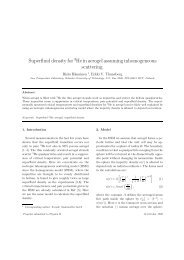
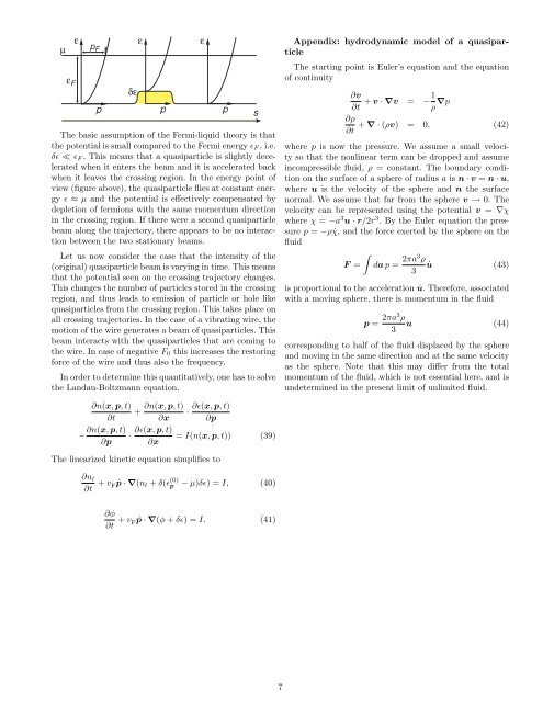
The basic assumption of the Fermi-liquid theory is that
the potential is small compared to the Fermi energy ɛF , i.e.
δɛ ≪ ɛF . This means that a quasiparticle is slightly decelerated
when it enters the beam and it is accelerated back
when it leaves the crossing region. In the energy point of
view (figure above), the quasiparticle flies at constant energy
ɛ ≈ µ and the potential is effectively compensated by
depletion of fermions with the same momentum direction
in the crossing region. If there were a second quasiparticle
beam along the trajectory, there appears to be no interaction
between the two stationary beams.
Let us now consider the case that the intensity of the
(original) quasiparticle beam is varying in time. This means
that the potential seen on the crossing trajectory changes.
This changes the number of particles stored in the crossing
region, and thus leads to emission of particle or hole like
quasiparticles from the crossing region. This takes place on
all crossing trajectories. In the case of a vibrating wire, the
motion of the wire generates a beam of quasiparticles. This
beam interacts with the quasiparticles that are coming to
the wire. In case of negative F0 this increases the restoring
force of the wire and thus also the frequency.
In order to determine this quantitatively, one has to solve
the Landau-Boltzmann equation.
∂n(x, p, t)
+
∂t
∂n(x, p, t)
·
∂x
∂ɛ(x, p, t)
∂p
∂n(x, p, t)
− ·
∂p
∂ɛ(x, p, t)
= I(n(x, p, t)) (39)
∂x
The linearized kinetic equation simplifies to
∂nl
∂t + v F ˆp · ∇(nl + δ(ɛ (0)
p − µ)δɛ) = I, (40)
∂φ
∂t + vF ˆp · ∇(φ + δɛ) = I. (41)
ε
p
s
7
Appendix: hydrodynamic model of a quasiparticle
The starting point is Euler’s equation and the equation
of continuity
∂v
+ v · ∇v
∂t
=
1
−
ρ ∇p
∂ρ
+ ∇ · (ρv)
∂t
= 0, (42)
where p is now the pressure. We assume a small velocity
so that the nonlinear term can be dropped and assume
incompressible fluid, ρ = constant. The boundary condition
on the surface of a sphere of radius a is n · v = n · u,
where u is the velocity of the sphere and n the surface
normal. We assume that far from the sphere v → 0. The
velocity can be represented using the potential v = ∇χ
where χ = −a3u · r/2r3 . By the Euler equation the pressure
p = −ρ ˙χ, and the force exerted by the sphere on the
fluid
F =
da p = 2πa3 ρ
3
˙u (43)
is proportional to the acceleration ˙u. Therefore, associated
with a moving sphere, there is momentum in the fluid
p = 2πa3ρ u (44)
3
corresponding to half of the fluid displaced by the sphere
and moving in the same direction and at the same velocity
as the sphere. Note that this may differ from the total
momentum of the fluid, which is not essential here, and is
undetermined in the present limit of unlimited fluid.