ESC-210: Introduction to Video Compression - DAIICT Intranet
ESC-210: Introduction to Video Compression - DAIICT Intranet
ESC-210: Introduction to Video Compression - DAIICT Intranet

Create successful ePaper yourself
Turn your PDF publications into a flip-book with our unique Google optimized e-Paper software.
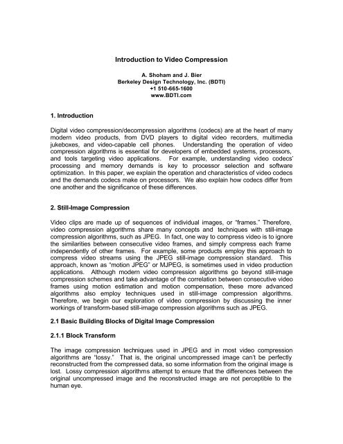
1. <strong>Introduction</strong><br />
<strong>Introduction</strong> <strong>to</strong> <strong>Video</strong> <strong>Compression</strong><br />
A. Shoham and J. Bier<br />
Berkeley Design Technology, Inc. (BDTI)<br />
+1 510-665-1600<br />
www.BDTI.com<br />
Digital video compression/decompression algorithms (codecs) are at the heart of many<br />
modern video products, from DVD players <strong>to</strong> digital video recorders, multimedia<br />
jukeboxes, and video-capable cell phones. Understanding the operation of video<br />
compression algorithms is essential for developers of embedded systems, processors,<br />
and <strong>to</strong>ols targeting video applications. For example, understanding video codecs’<br />
processing and memory demands is key <strong>to</strong> processor selection and software<br />
optimization. In this paper, we explain the operation and characteristics of video codecs<br />
and the demands codecs make on processors. We also explain how codecs differ from<br />
one another and the significance of these differences.<br />
2. Still-Image <strong>Compression</strong><br />
<strong>Video</strong> clips are made up of sequences of individual images, or “frames.” Therefore,<br />
video compression algorithms share many concepts and techniques with still-image<br />
compression algorithms, such as JPEG. In fact, one way <strong>to</strong> compress video is <strong>to</strong> ignore<br />
the similarities between consecutive video frames, and simply compress each frame<br />
independently of other frames. For example, some products employ this approach <strong>to</strong><br />
compress video streams using the JPEG still-image compression standard. This<br />
approach, known as “motion JPEG” or MJPEG, is sometimes used in video production<br />
applications. Although modern video compression algorithms go beyond still-image<br />
compression schemes and take advantage of the correlation between consecutive video<br />
frames using motion estimation and motion compensation, these more advanced<br />
algorithms also employ techniques used in still-image compression algorithms.<br />
Therefore, we begin our exploration of video compression by discussing the inner<br />
workings of transform-based still-image compression algorithms such as JPEG.<br />
2.1 Basic Building Blocks of Digital Image <strong>Compression</strong><br />
2.1.1 Block Transform<br />
The image compression techniques used in JPEG and in most video compression<br />
algorithms are “lossy.” That is, the original uncompressed image can’t be perfectly<br />
reconstructed from the compressed data, so some information from the original image is<br />
lost. Lossy compression algorithms attempt <strong>to</strong> ensure that the differences between the<br />
original uncompressed image and the reconstructed image are not perceptible <strong>to</strong> the<br />
human eye.
The first step in JPEG and similar image compression algorithms is <strong>to</strong> divide the image<br />
in<strong>to</strong> small blocks and transform each block in<strong>to</strong> a frequency-domain representation.<br />
Typically, this step uses a discrete cosine transform (DCT) on blocks that are eight<br />
pixels wide by eight pixels high. Thus, the DCT operates on 64 input pixels and yields<br />
64 frequency-domain coefficients. The DCT itself preserves all of the information in the<br />
eight-by-eight image block. That is, an inverse DCT (IDCT) can be used <strong>to</strong> perfectly<br />
reconstruct the original 64 pixels from the DCT coefficients. However, the human eye is<br />
more sensitive <strong>to</strong> the information contained in DCT coefficients that represent low<br />
frequencies (corresponding <strong>to</strong> large features in the image) than <strong>to</strong> the information<br />
contained in DCT coefficients that represent high frequencies (corresponding <strong>to</strong> small<br />
features). Therefore, the DCT helps separate the more perceptually significant<br />
information from less perceptually significant information. Later steps in the compression<br />
algorithm encode the low-frequency DCT coefficients with high precision, but use fewer<br />
or no bits <strong>to</strong> encode the high-frequency coefficients, thus discarding information that is<br />
less perceptually significant. In the decoding algorithm, an IDCT transforms the<br />
imperfectly coded coefficients back in<strong>to</strong> an 8x8 block of pixels.<br />
The computations performed in the IDCT are nearly identical <strong>to</strong> those performed in the<br />
DCT, so these two functions have very similar processing requirements. A single twodimensional<br />
eight-by-eight DCT or IDCT requires a few hundred instruction cycles on a<br />
typical DSP. However, video compression algorithms must often perform a vast number<br />
of DCTs and/or IDCTs per second. For example, an MPEG-4 video decoder operating<br />
at CIF (352x288) resolution and a frame rate of 30 fps may need <strong>to</strong> perform as many as<br />
71,280 IDCTs per second, depending on the video content. The IDCT function would<br />
require over 40 MHz on a Texas Instruments TMS320C55x DSP processor (without the<br />
DCT accelera<strong>to</strong>r) under these conditions. IDCT computation can take up as much as<br />
30% of the cycles spent in a video decoder implementation.<br />
Because the DCT and IDCT operate on small image blocks, the memory requirements<br />
of these functions are rather small and are typically negligible compared <strong>to</strong> the size of<br />
frame buffers and other data in image and video compression applications. The high<br />
computational demand and small memory footprint of the DCT and IDCT functions make<br />
them ideal candidates for implementation using dedicated hardware coprocessors.<br />
2.1.2 Quantization<br />
As mentioned above, the DCT coefficients for each eight-pixel by eight-pixel block are<br />
encoded using more bits for the more perceptually significant low-frequency DCT<br />
coefficients and fewer bits for the less significant high-frequency coefficients. This<br />
encoding of coefficients is accomplished in two steps: First, quantization is used <strong>to</strong><br />
discard perceptually insignificant information. Next, statistical methods are used <strong>to</strong><br />
encode the remaining information using as few bits as possible.<br />
Quantization rounds each DCT coefficient <strong>to</strong> the nearest of a number of predetermined<br />
values. For example, if the DCT coefficient is a real number between -1 and 1, then<br />
scaling the coefficient by 20 and rounding <strong>to</strong> the nearest integer quantizes the coefficient<br />
<strong>to</strong> the nearest of 41 steps, represented by the integers from -20 <strong>to</strong> +20. Ideally, for each<br />
DCT coefficient a scaling fac<strong>to</strong>r is chosen so that information contained in the digits <strong>to</strong><br />
the right of the decimal point of the scaled coefficient may be discarded without<br />
introducing perceptible artifacts <strong>to</strong> the image.
In the image decoder, dequantization performs the inverse of the scaling applied in the<br />
encoder. In the example above, the quantized DCT coefficient would be scaled by 1/20,<br />
resulting in a dequantized value between -1 and 1. Note that the dequantized<br />
coefficients are not equal <strong>to</strong> the original coefficients, but are close enough so that after<br />
the IDCT is applied, the resulting image contains few or no visible artifacts.<br />
Dequantization can require anywhere from about 3% up <strong>to</strong> about 15% of the processor<br />
cycles spent in a video decoding application. Like the DCT and IDCT, the memory<br />
requirements of quantization and dequantization are typically negligible.<br />
2.1.3 Coding<br />
The next step in the compression process is <strong>to</strong> encode the quantized DCT coefficients in<br />
the digital bit stream using as few bits as possible. The number of bits used for<br />
encoding the quantized DCT coefficients can be minimized by taking advantage of some<br />
statistical properties of the quantized coefficients.<br />
After quantization, many of the DCT coefficients have a value of zero. In fact, this is<br />
often true for the vast majority of high-frequency DCT coefficients. A technique called<br />
“run-length coding” takes advantage of this fact by grouping consecutive zero-valued<br />
coefficients (a “run“) and encoding the number of coefficients (the “length”) instead of<br />
encoding the individual zero-valued coefficients.<br />
To maximize the benefit of run-length coding, low-frequency DCT coefficients are<br />
encoded first, followed by higher-frequency coefficients, so that the average number of<br />
consecutive zero-valued coefficients is as high as possible. This is accomplished by<br />
scanning the eight-by-eight-coefficient matrix in a diagonal zig-zag pattern.<br />
Run-length coding is typically followed by variable-length coding (VLC). In variablelength<br />
coding, each possible value of an item of data (i.e., each possible run length or<br />
each possible value of a quantized DCT coefficient) is called a symbol. Commonly<br />
occurring symbols are represented using code words that contain only a few bits, while<br />
less common symbols are represented with longer code words. VLC uses fewer bits for<br />
the most common symbols compared <strong>to</strong> fixed-length codes (e.g. directly encoding the<br />
quantized DCT coefficients as binary integers) so that on average, VLC requires fewer<br />
bits <strong>to</strong> encode the entire image. Huffman coding is a variable-length coding scheme that<br />
optimizes the number of bits in each code word based on the frequency of occurrence of<br />
each symbol.<br />
Note that theoretically, VLC is not the most efficient way <strong>to</strong> encode a sequence of<br />
symbols. A technique called “arithmetic coding” can encode a sequence of symbols<br />
using fewer bits than VLC. Arithmetic coding is more efficient because it encodes the<br />
entire sequence of symbols <strong>to</strong>gether, instead of using individual code words whose<br />
lengths must each be an integer number of bits. Arithmetic coding is more<br />
computationally demanding than VLC and has only recently begun <strong>to</strong> make its way in<strong>to</strong><br />
commercially available video compression algorithms. His<strong>to</strong>rically, the combination of<br />
run-length coding and VLC has provided sufficient coding efficiency with much lower<br />
computational requirements than arithmetic coding, so VLC is the coding method used in<br />
the vast majority of video compression algorithms available <strong>to</strong>day.
Variable-length coding is implemented by retrieving code words and their lengths from<br />
lookup tables, and appending the code word bits <strong>to</strong> the output bit stream. The<br />
corresponding variable-length decoding process (VLD) is much more computationally<br />
intensive. Compared <strong>to</strong> performing a table lookup per symbol in the encoder, the most<br />
straightforward implementation of VLD requires a table lookup and some simple decision<br />
making <strong>to</strong> be applied for each bit. VLD requires an average of about 11 operations per<br />
input bit. Thus, the processing requirements of VLD are proportional <strong>to</strong> the video<br />
compression codec’s selected bit rate. Note that for low image resolutions and frame<br />
rates, VLD can sometimes consume as much as 25% of the cycles spent in a video<br />
decoder implementation.<br />
In a typical video decoder, the straightforward VLD implementation described above<br />
requires several kilobytes of lookup table memory. VLD performance can be greatly<br />
improved by operating on multiple bits at a time. However, such optimizations require<br />
the use of much larger lookup tables.<br />
One drawback of variable-length codes is that a bit error in the middle of an encoded<br />
image or video frame can prevent the decoder from correctly reconstructing the portion<br />
of the image that is encoded after the corrupted bit. Upon detection of an error, the<br />
decoder can no longer determine the start of the next variable-length code word in the<br />
bit stream, because the correct length of the corrupted code word is not known. Thus,<br />
the decoder cannot continue decoding the image. One technique that video<br />
compression algorithms use <strong>to</strong> mitigate this problem is <strong>to</strong> intersperse “resynchronization<br />
markers” throughout the encoded bit stream. Resynchronization markers occur at<br />
predefined points in the bit stream and provide a known bit pattern that the video<br />
decoder can detect. In the event of an error, the decoder is able <strong>to</strong> search for the next<br />
resynchronization marker following the error, and continue decoding the portion of the<br />
frame that follows the resynchronization marker.<br />
In addition, the MPEG-4 video compression standard employs “reversible” variablelength<br />
codes. Reversible variable-length codes use code words carefully chosen so that<br />
they can be uniquely decoded both in the normal forward direction, and also backwards.<br />
In the event of an error, the use of reversible codes allows the video decoder <strong>to</strong> find the<br />
resynchronization marker following the error and decode the bit stream in the backward<br />
direction from the resynchronization marker <strong>to</strong>ward the error. Thus, the decoder can<br />
recover more of the image data than would be possible with resynchronization markers<br />
alone.<br />
All of the techniques described so far operate on each eight-pixel by eight-pixel block<br />
independently from any other block. Since images typically contain features that are<br />
much larger than an eight-by-eight block, more efficient compression can be achieved by<br />
taking in<strong>to</strong> account the correlation between adjacent blocks in the image.<br />
To take advantage of inter-block correlation, a prediction step is often added prior <strong>to</strong><br />
quantization of the DCT coefficients. In this step, the encoder attempts <strong>to</strong> predict the<br />
values of some of the DCT coefficients in each block based on the DCT coefficients of<br />
the surrounding blocks. Instead of quantizing and encoding the DCT coefficients<br />
directly, the encoder computes, quantizes, and encodes the difference between the<br />
actual DCT coefficients and the predicted values of those coefficients. Because the<br />
difference between the predicted and actual values of the DCT coefficients tends <strong>to</strong> be<br />
small, this technique reduces the number of bits needed for the DCT coefficients. The
decoder performs the same prediction as the encoder, and adds the differences<br />
encoded in the compressed bit stream <strong>to</strong> the predicted coefficients in order <strong>to</strong><br />
reconstruct the actual DCT coefficient values. Note that in predicting the DCT coefficient<br />
values of a particular block, the decoder has access only <strong>to</strong> the DCT coefficients of<br />
surrounding blocks that have already been decoded. Therefore, the encoder must<br />
predict the DCT coefficients of each block based only on the coefficients of previously<br />
encoded surrounding blocks.<br />
In the simplest case, only the first DCT coefficient of each block is predicted. This<br />
coefficient, called the “DC coefficient,” is the lowest frequency DCT coefficient and<br />
equals the average of all the pixels in the block. All other coefficients are called “AC<br />
coefficients.” The simplest way <strong>to</strong> predict the DC coefficient of an image block is <strong>to</strong><br />
simply assume that it is equal <strong>to</strong> the DC coefficient of the adjacent block <strong>to</strong> the left of the<br />
current block. This adjacent block is typically the previously encoded block. In the<br />
simplest case, therefore, taking advantage of some of the correlation between image<br />
blocks amounts <strong>to</strong> encoding the difference between the DC coefficient of the current<br />
block and the DC coefficient of the previously encoded block instead of encoding the DC<br />
coefficient values directly. This practice is referred <strong>to</strong> as “differential coding of DC<br />
coefficients” and is used in the JPEG image compression algorithm.<br />
More sophisticated prediction schemes attempt <strong>to</strong> predict the first DCT coefficient in<br />
each row and each column of the eight-by-eight block. Such schemes are referred <strong>to</strong> as<br />
“AC-DC prediction” and often use more sophisticated prediction methods compared <strong>to</strong><br />
the differential coding method described above: First, a simple filter may be used <strong>to</strong><br />
predict each coefficient value instead of assuming that the coefficient is equal <strong>to</strong> the<br />
corresponding coefficient from an adjacent block. Second, the prediction may consider<br />
the coefficient values from more than one adjacent block. The prediction can be based<br />
on the combined data from several adjacent blocks. Alternatively, the encoder can<br />
evaluate all of the previously encoded adjacent blocks and select the one that yields the<br />
best predictions on average. In the latter case, the encoder must specify in the bit<br />
stream which adjacent block was selected for prediction so that the decoder can perform<br />
the same prediction <strong>to</strong> correctly reconstruct the DCT coefficients.<br />
AC-DC prediction can take a substantial number of processor cycles when decoding a<br />
single image. However, AC-DC prediction cannot be used in conjunction with motion<br />
compensation. Therefore, in video compression applications AC-DC prediction is only<br />
used a small fraction of the time and usually has a negligible impact on processor load.<br />
However, some implementations of AC-DC prediction use large arrays of data. Often it<br />
may be possible <strong>to</strong> overlap these arrays with other memory structures that are not in use<br />
during AC-DC prediction <strong>to</strong> dramatically optimize the video decoder’s memory use.<br />
2.2 A Note About Color<br />
Color images are typically represented using several “color planes.” For example, an<br />
RGB color image contains a red color plane, a green color plane, and a blue color plane.<br />
Each plane contains an entire image in a single color (red, green, or blue, respectively).<br />
When overlaid and mixed, the three planes make up the full color image. To compress a<br />
color image, the still-image compression techniques described here are applied <strong>to</strong> each<br />
color plane in turn.
<strong>Video</strong> applications often use a color scheme in which the color planes do not correspond<br />
<strong>to</strong> specific colors. Instead, one color plane contains luminance information (the overall<br />
brightness of each pixel in the color image) and two more color planes contain color<br />
(chrominance) information that when combined with luminance can be used <strong>to</strong> derive the<br />
specific levels of the red, green, and blue components of each image pixel.<br />
Such a color scheme is convenient because the human eye is more sensitive <strong>to</strong><br />
luminance than <strong>to</strong> color, so the chrominance planes are often s<strong>to</strong>red and encoded at a<br />
lower image resolution than the luminance information. Specifically, video compression<br />
algorithms typically encode the chrominance planes with half the horizontal resolution<br />
and half the vertical resolution as the luminance plane. Thus, for every 16-pixel by 16pixel<br />
region in the luminance plane, each chrominance plane contains one eight-pixel by<br />
eight-pixel block. In typical video compression algorithms, a “macro block” is a 16-pixel<br />
by 16-pixel region in the video frame that contains four eight-by-eight luminance blocks<br />
and the two corresponding eight-by-eight chrominance blocks. Macro blocks allow<br />
motion estimation and compensation, described below, <strong>to</strong> be used in conjunction with<br />
sub-sampling of the chrominance planes as described above.<br />
3. Adding Motion <strong>to</strong> the Mix<br />
Using the techniques described above, still-image compression algorithms such as<br />
JPEG can achieve good image quality at a compression ratio of about 10:1. The most<br />
advanced still-image coders may achieve good image quality at compression ratios as<br />
high as 30:1. <strong>Video</strong> compression algorithms, however, employ motion estimation and<br />
compensation <strong>to</strong> take advantage of the similarities between consecutive video frames.<br />
This allows video compression algorithms <strong>to</strong> achieve good video quality at compression<br />
ratios up <strong>to</strong> 200:1.<br />
In some video scenes, such as a news program, little motion occurs. In this case, the<br />
majority of the eight-pixel by eight-pixel blocks in each video frame are identical or nearly<br />
identical <strong>to</strong> the corresponding blocks in the previous frame. A compression algorithm<br />
can take advantage of this fact by computing the difference between the two frames, and<br />
using the still-image compression techniques described above <strong>to</strong> encode this difference.<br />
Because the difference is small for most of the image blocks, it can be encoded with<br />
many fewer bits than would be required <strong>to</strong> encode each frame independently. If the<br />
camera pans or large objects in the scene move, however, then each block no longer<br />
corresponds <strong>to</strong> the same block in the previous frame. Instead, each block is similar <strong>to</strong><br />
an eight-pixel by eight-pixel region in the previous frame that is offset from the block’s<br />
location by a distance that corresponds <strong>to</strong> the motion in the image. Note that each video<br />
frame is typically composed of a luminance plane and two chrominance planes as<br />
described above. Obviously, the motion in each of the three planes is the same. To<br />
take advantage of this fact despite the different resolutions of the luminance and<br />
chrominance planes, motion is analyzed in terms of macro blocks rather than working<br />
with individual eight-by-eight blocks in each of the three planes.<br />
3.1 Motion Estimation and Compensation<br />
Motion estimation attempts <strong>to</strong> find a region in a previously encoded frame (called a<br />
“reference frame”) that closely matches each macro block in the current frame. For each<br />
macro block, motion estimation results in a “motion vec<strong>to</strong>r.” The motion vec<strong>to</strong>r is
comprised of the horizontal and vertical offsets from the location of the macro block in<br />
the current frame <strong>to</strong> the location in the reference frame of the selected 16-pixel by 16pixel<br />
region. The video encoder typically uses VLC <strong>to</strong> encode the motion vec<strong>to</strong>r in the<br />
video bit stream. The selected 16-pixel by 16-pixel region is used as a prediction of the<br />
pixels in the current macro block, and the difference between the macro block and the<br />
selected region (the “prediction error”) is computed and encoded using the still-image<br />
compression techniques described above. Most video compression standards allow this<br />
prediction <strong>to</strong> be bypassed if the encoder fails <strong>to</strong> find a good enough match for the macro<br />
block. In this case, the macro block itself is encoded instead of the prediction error.<br />
Note that the reference frame isn’t always the previously displayed frame in the<br />
sequence of video frames. <strong>Video</strong> compression algorithms commonly encode frames in<br />
a different order from the order in which they are displayed. The encoder may skip<br />
several frames ahead and encode a future video frame, then skip backward and encode<br />
the next frame in the display sequence. This is done so that motion estimation can be<br />
performed backward in time, using the encoded future frame as a reference frame.<br />
<strong>Video</strong> compression algorithms also commonly allow the use of two reference frames—<br />
one previously displayed frame and one previously encoded future frame. This allows<br />
the encoder <strong>to</strong> select a 16-pixel by 16-pixel region from either reference frame, or <strong>to</strong><br />
predict a macro block by interpolating between a 16-pixel by 16-pixel region in the<br />
previously displayed frame and a 16-pixel by 16-pixel region in the future frame.<br />
One drawback of relying on previously encoded frames for correct decoding of each<br />
new frame is that errors in the transmission of a frame make every subsequent frame<br />
impossible <strong>to</strong> reconstruct. To alleviate this problem, video compression standards<br />
occasionally encode one video frame using still-image coding techniques only, without<br />
relying on previously encoded frames. These frames are called “intra frames” or “Iframes.”<br />
If a frame in the compressed bit stream is corrupted by errors the video<br />
decoder must wait until the next I-frame, which doesn’t require a reference frame for<br />
reconstruction.<br />
Frames that are encoded using only a previously displayed reference frame are called<br />
“P-frames,” and frames that are encoded using both future and previously displayed<br />
reference frames are called “B-frames.” In a typical scenario, the codec encodes an Iframe,<br />
skips several frames ahead and encodes a future P-frame using the encoded Iframe<br />
as a reference frame, then skips back <strong>to</strong> the next frame following the I-frame. The<br />
frames between the encoded I- and P-frames are encoded as B-frames. Next, the<br />
encoder skips several frames again, encoding another P-frame using the first P-frame as<br />
a reference frame, then once again skips back <strong>to</strong> fill in the gap in the display sequence<br />
with B-frames. This process continues, with a new I-frame inserted for every 12 <strong>to</strong> 15 P-<br />
and B-frames. For example, a typical sequence of frames is illustrated in Figure 1.<br />
Encoding<br />
Order<br />
(<strong>to</strong>p <strong>to</strong><br />
bot<strong>to</strong>m)<br />
Display Order (left <strong>to</strong> right)<br />
I<br />
P<br />
B<br />
B<br />
B<br />
B<br />
P
Figure 1. A typical sequence of I, P, and B frames.<br />
<strong>Video</strong> compression standards sometimes restrict the size of the horizontal and vertical<br />
components of a motion vec<strong>to</strong>r so that the maximum possible distance between each<br />
macro block and the 16-pixel by 16-pixel region selected during motion estimation is<br />
much smaller than the width or height of the frame. This restriction slightly reduces the<br />
number of bits needed <strong>to</strong> encode motion vec<strong>to</strong>rs, and can also reduce the amount of<br />
computation required <strong>to</strong> perform motion estimation. The portion of the reference frame<br />
that contains all possible 16-by-16 regions that are within the reach of the allowable<br />
motion vec<strong>to</strong>rs is called the “search area.”<br />
In addition, modern video compression standards allow motion vec<strong>to</strong>rs <strong>to</strong> have noninteger<br />
values. That is, the encoder may estimate that the motion between the reference<br />
frame and current frame for a given macro block is not an integer number of pixels.<br />
Motion vec<strong>to</strong>r resolutions of one-half or one-quarter of a pixel are common. Thus, <strong>to</strong><br />
predict the pixels in the current macro block, the corresponding region in the reference<br />
frame must be interpolated <strong>to</strong> estimate the pixel values at non-integer pixel locations.<br />
The difference between this prediction and the actual pixel values is computed and<br />
encoded as described above.<br />
Motion estimation is the most computationally demanding task in image compression<br />
applications, and can require as much as 80% of the processor cycles spent in the video<br />
encoder. The simplest and most thorough way <strong>to</strong> perform motion estimation is <strong>to</strong><br />
evaluate every possible 16-by-16 region in the search area, and select the best match.<br />
Typically, a “sum of absolute differences” (SAD) or “sum of squared differences” (SSD)<br />
computation is used <strong>to</strong> determine how closely a 16-pixel by 16-pixel region matches a<br />
macro block. The SAD or SSD is often computed for the luminance plane only, but can<br />
also include the chrominance planes. A relatively small search area of 48 pixels by 24<br />
pixels, for example, contains 1024 possible 16-by-16 regions at ½-pixel resolution.<br />
Performing an SAD on the luminance plane only for one such region requires 256<br />
subtractions, 256 absolute value operations, and 255 additions. Thus, not including the<br />
interpolation required for non-integer motion vec<strong>to</strong>rs, the SAD computations needed <strong>to</strong><br />
exhaustively scan this search area for the best match require a <strong>to</strong>tal of 785,408<br />
arithmetic operations per macro block, which equates <strong>to</strong> over 4.6 billion arithmetic<br />
operations per second at CIF (352 by 288 pixels) video resolution and a modest frame<br />
rate of 15 frames per second.<br />
Because of this high computational load, practical implementations of motion estimation<br />
do not use an exhaustive search. Instead, motion estimation algorithms use various<br />
methods <strong>to</strong> select a limited number of promising candidate motion vec<strong>to</strong>rs (roughly 10 <strong>to</strong><br />
100 vec<strong>to</strong>rs in most cases) and evaluate only the 16-pixel by 16-pixel regions<br />
corresponding <strong>to</strong> these candidate vec<strong>to</strong>rs. One approach is <strong>to</strong> select the candidate<br />
motion vec<strong>to</strong>rs in several stages. For example, five initial candidate vec<strong>to</strong>rs may be<br />
B<br />
B<br />
B<br />
B<br />
B<br />
P<br />
I
selected and evaluated. The results are used <strong>to</strong> eliminate unlikely portions of the search<br />
area and hone in on the most promising portion of the search area. Five new vec<strong>to</strong>rs<br />
are selected and the process is repeated. After a few such stages, the best motion<br />
vec<strong>to</strong>r found so far is selected.<br />
Another approach analyzes the motion vec<strong>to</strong>rs selected for surrounding macro blocks in<br />
the current and previous frames in the video sequence in an effort <strong>to</strong> predict the motion<br />
in the current macro block. A handful of candidate motion vec<strong>to</strong>rs are selected based on<br />
this analysis, and only these vec<strong>to</strong>rs are evaluated.<br />
By selecting a small number of candidate vec<strong>to</strong>rs instead of scanning the search area<br />
exhaustively, the computational demand of motion estimation can be reduced<br />
considerably, sometimes by over two orders of magnitude. Note that there is a tradeoff<br />
between computational demand and image quality and/or compression efficiency: using<br />
a larger number of candidate motion vec<strong>to</strong>rs allows the encoder <strong>to</strong> find a 16-pixel by 16pixel<br />
region in the reference frame that better matches each macro block, thus reducing<br />
the prediction error. Therefore, increasing the number of candidate vec<strong>to</strong>rs on average<br />
allows the prediction error <strong>to</strong> be encoded with fewer bits or higher precision, at the cost<br />
of performing more SAD (or SSD) computations.<br />
In addition <strong>to</strong> the two approaches describe above, many other methods for selecting<br />
appropriate candidate motion vec<strong>to</strong>rs exist, including a wide variety of proprietary<br />
solutions. Most video compression standards specify only the format of the compressed<br />
video bit stream and the decoding steps, and leave the encoding process undefined so<br />
that encoders can employ a variety of approaches <strong>to</strong> motion estimation. The approach<br />
<strong>to</strong> motion estimation is the largest differentia<strong>to</strong>r among video encoder implementations<br />
that comply with a common standard. The choice of motion estimation technique<br />
significantly impacts computational requirements and video quality; therefore, details of<br />
the approach <strong>to</strong> motion estimation in commercially available encoders are often closely<br />
guarded trade secrets.<br />
Many processors targeting multimedia applications provide a specialized instruction <strong>to</strong><br />
accelerate SAD computations, or a dedicated SAD coprocessor <strong>to</strong> offload this<br />
computationally demanding task from the CPU.<br />
Note that in order <strong>to</strong> perform motion estimation, the encoder must keep one or two<br />
reference frames in memory in addition <strong>to</strong> the current frame. The required frame buffers<br />
are very often larger than the available on-chip memory, requiring additional memory<br />
chips in many applications. Keeping reference frames in off-chip memory results in very<br />
high external memory bandwidth in the encoder, although large on-chip caches can help<br />
reduce the required bandwidth considerably.<br />
Some video compression standards allow each macro block <strong>to</strong> be divided in<strong>to</strong> two or<br />
four subsections, and a separate motion vec<strong>to</strong>r is found for each subsection. This option<br />
requires more bits <strong>to</strong> encode the two or four motion vec<strong>to</strong>rs for the macro block<br />
compared <strong>to</strong> the default of one motion vec<strong>to</strong>r. However, this may be a worthwhile<br />
tradeoff if the additional motion vec<strong>to</strong>rs provide a better prediction of the macro block<br />
pixels and results in fewer bits used for the encoding of the prediction error.
3.2 Motion Compensation<br />
In the video decoder, motion compensation uses the motion vec<strong>to</strong>rs encoded in the<br />
video bit stream <strong>to</strong> predict the pixels in each macro block. If the horizontal and vertical<br />
components of the motion vec<strong>to</strong>r are both integer values, then the predicted macro block<br />
is simply a copy of the 16-pixel by 16-pixel region of the reference frame. If either<br />
component of the motion vec<strong>to</strong>r has a non-integer value, interpolation is used <strong>to</strong><br />
estimate the image at non-integer pixel locations. Next, the prediction error is decoded<br />
and added <strong>to</strong> the predicted macro block in order <strong>to</strong> reconstruct the actual macro block<br />
pixels.<br />
Compared <strong>to</strong> motion estimation, motion compensation is much less computationally<br />
demanding. While motion estimation must perform SAD or SSD computation on a<br />
number of 16-pixel by 16-pixel regions per macro block, motion compensation simply<br />
copies or interpolates one such region. Because of this important difference, video<br />
decoding is much less computationally demanding than encoding. Nevertheless, motion<br />
compensation can still take up as much as 40% of the processor cycles in a video<br />
decoder, although this number varies greatly depending on the content of a video<br />
sequence, the video compression standard, and the decoder implementation. For<br />
example, the motion compensation workload can comprise as little as 5% of the<br />
processor cycles spent in the decoder for a frame that makes little use of interpolation.<br />
Like motion estimation, motion compensation requires the video decoder <strong>to</strong> keep one or<br />
two reference frames in memory, often requiring external memory chips for this purpose.<br />
However, motion compensation makes fewer accesses <strong>to</strong> reference frame buffers than<br />
does motion estimation. Therefore, memory bandwidth requirements are less stringent<br />
for motion compensation compared <strong>to</strong> motion estimation, although high memory<br />
bandwidth is still desirable for best processor performance in motion compensation<br />
functions.<br />
4. Reducing Artifacts<br />
4.1 Blocking and Ringing Artifacts<br />
Ideally, lossy image and video compression algorithms discard only perceptually<br />
insignificant information, so that <strong>to</strong> the human eye the reconstructed image or video<br />
sequence appears identical <strong>to</strong> the original uncompressed image or video. In practice,<br />
however, some visible artifacts may occur. This can happen due <strong>to</strong> a poor encoder<br />
implementation, video content that is particularly challenging <strong>to</strong> encode, or a selected bit<br />
rate that is <strong>to</strong>o low for the video sequence resolution and frame rate. The latter case is<br />
particularly common, since many applications trade off video quality for a reduction in<br />
s<strong>to</strong>rage and/or bandwidth requirements.<br />
Two types of artifacts, “blocking” and “ringing,” are particularly common in video<br />
compression. Blocking artifacts are due <strong>to</strong> the fact that compression algorithms divide<br />
each frame in<strong>to</strong> eight-pixel by eight-pixel blocks. Each block is reconstructed with some<br />
small errors, and the errors at the edges of a block often contrast with the errors at the<br />
edges of neighboring blocks, making block boundaries visible. Ringing artifacts are due<br />
<strong>to</strong> the encoder discarding <strong>to</strong>o much information in quantizing the high-frequency DCT<br />
coefficients. Ringing artifacts appear as dis<strong>to</strong>rtions around the edges of image features.
4.2 Deblocking and Deringing Image Filters<br />
<strong>Video</strong> compression applications often employ filters following decompression <strong>to</strong> reduce<br />
blocking and ringing artifacts. These filtering steps are known as “deblocking” and<br />
“deringing,” respectively. Both deblocking and deringing utilize low-pass FIR (finite<br />
impulse response) filters <strong>to</strong> hide these visible artifacts. Deblocking filters are applied at<br />
the edges of image blocks, blending the edges of each block with those of its neighbors<br />
<strong>to</strong> hide blocking artifacts. Deringing often uses an adaptive filter. The deringing filter<br />
first detects the edges of image features. A low-pass filter is then applied <strong>to</strong> the areas<br />
near the detected edges <strong>to</strong> smooth away ringing artifacts, but the edge pixels<br />
themselves are left unfiltered or weakly filtered in order <strong>to</strong> avoid blurring.<br />
Deblocking and deringing filters are fairly computationally demanding. Combined, these<br />
filters can easily consume more processor cycles than the video decoder itself. For<br />
example, an MPEG-4 simple-profile, level 1 (176x144 pixel, 15 fps) decoder optimized<br />
for the ARM9E general-purpose processor core requires that the processor be run at an<br />
instruction cycle rate of about 14 MHz when decoding a moderately complex video<br />
stream. If deblocking is added, the processor must be run at 33 MHz. If deringing and<br />
deblocking are both added, the processor must be run at about 39 MHz—nearly three<br />
times the clock rate required for the video decompression algorithm alone.<br />
4.3 Post-processing vs. In-line Implementation<br />
Deblocking and deringing filters can be applied <strong>to</strong> video frames as a separate postprocessing<br />
step that is independent of video decompression. This approach provides<br />
system designers the flexibility <strong>to</strong> select the best deblocking and/or deringing filters for<br />
their application, or <strong>to</strong> forego these filters entirely in order <strong>to</strong> reduce computational<br />
demands. With this approach, the video decoder uses each unfiltered reconstructed<br />
frame as a reference frame for decoding future video frames, and an additional frame<br />
buffer is required for the final filtered video output.<br />
Alternatively, deblocking and/or deringing can be integrated in<strong>to</strong> the video<br />
decompression algorithm. This approach, sometimes referred <strong>to</strong> as “loop filtering,” uses<br />
the filtered reconstructed frame as the reference frame for decoding future video frames.<br />
This approach requires the video encoder <strong>to</strong> perform the same deblocking and/or<br />
deringing filtering steps as the decoder, in order <strong>to</strong> keep each reference frame used in<br />
encoding identical <strong>to</strong> that used in decoding. The need <strong>to</strong> perform filtering in the encoder<br />
increases processor performance requirements for encoding, but can improve image<br />
quality, especially for very low bit rates. In addition, the extra frame buffer that is<br />
required when deblocking and/or deringing are implemented as a separate postprocessing<br />
step is not needed when deblocking and deringing are integrated in<strong>to</strong> the<br />
decompression algorithm .<br />
5. Color Space Conversion<br />
As noted above, video compression algorithms typically represent color images using<br />
luminance and chrominance planes. In contrast, video cameras and displays typically<br />
mix red, green, and blue light <strong>to</strong> represent different colors. Therefore, the red, green,<br />
and blue pixels captured by a camera must be converted in<strong>to</strong> luminance and
chrominance values for video encoding, and the luminance and chrominance pixels<br />
output by the video decoder must be converted <strong>to</strong> specific levels of red, green, and blue<br />
for display. The equations for this conversion require about 12 arithmetic operations per<br />
image pixel, not including the interpolation needed <strong>to</strong> compensate for the fact that the<br />
chrominance planes have a lower resolution than the luminance plane at the video<br />
compression algorithm’s input and output. For a CIF (352 by 288 pixel) image resolution<br />
at 15 frames per second, conversion (without any interpolation) requires over 18 million<br />
operations per second. This computational load can be significant; when implemented<br />
in software, color conversion requires roughly one-third <strong>to</strong> two-thirds as many processor<br />
cycles as the video decoder.<br />
6. Summary and Conclusions<br />
<strong>Video</strong> compression algorithms employ a variety of signal-processing tasks such as<br />
motion estimation, transforms, and variable-length coding. Although most modern video<br />
compression algorithms share these basic tasks, there is enormous variation among<br />
algorithms and implementation techniques. For example, the algorithmic approaches<br />
and implementation techniques used for performing motion estimation can vary among<br />
video encoders even when the encoders comply with the same compression standard.<br />
In addition, the most efficient implementation approach for a given signal-processing<br />
task can differ considerably from one processor <strong>to</strong> another, even when a similar<br />
algorithmic approach is used on each processor. Finally, the computational load of some<br />
tasks, such as motion compensation, can fluctuate wildly depending on the video<br />
program content. Therefore, the computational load of a video encoder or decoder on a<br />
particular processor can be difficult <strong>to</strong> predict.<br />
Despite this variability, a few trends can readily be observed:<br />
• Motion estimation is by far the most computationally demanding task in the video<br />
compression process, often making the computational load of the encoder several times<br />
greater than that of the decoder.<br />
• The computational load of the decoder is typically dominated by the variablelength<br />
decoding, inverse transform, and motion compensation functions.<br />
• The computational load of motion estimation, motion compensation, transform,<br />
and quantization/dequantization tasks is generally proportional <strong>to</strong> the number of<br />
pixels per frame and <strong>to</strong> the frame rate. In contrast, the computational load of the<br />
variable-length decoding function is proportional <strong>to</strong> the bit rate of the compressed<br />
video bit stream.<br />
• Post-processing steps applied <strong>to</strong> the video stream after decoding—namely,<br />
deblocking, deringing, and color space conversion—contribute considerably <strong>to</strong><br />
the computational load of video decoding applications. The computational load<br />
of these functions can easily exceed that of the video decompression step, and is<br />
proportional <strong>to</strong> the number of pixels per frame and <strong>to</strong> the frame rate.<br />
The memory requirements of a video compression application are much easier <strong>to</strong> predict<br />
than its computational load: in video compression applications memory use is dominated
y the large buffers used <strong>to</strong> s<strong>to</strong>re the current and reference video frames. Only two<br />
frame buffers are needed if the compression scheme supports only I- and P-frames;<br />
three frame buffers are needed if B-frames are also supported. Post-processing steps<br />
such as deblocking, deringing, and color space conversion may require an additional<br />
output buffer. The size of these buffers is proportional <strong>to</strong> the number of pixels per frame.<br />
Combined, other fac<strong>to</strong>rs such as program memory, lookup tables, and intermediate data<br />
comprise a significant portion of a typical video application’s memory use, although this<br />
portion is often still several times smaller than the frame buffer memory.<br />
Implementing highly optimized video encoding and decoding software requires a<br />
thorough understanding of the signal-processing concepts introduced in this paper and<br />
of the target processor. Most video compression standards do not specify the method for<br />
performing motion estimation. Although reference encoder implementations are<br />
provided for most standards, in-depth understanding of video compression algorithms<br />
often allows designers <strong>to</strong> utilize more sophisticated motion estimation methods and<br />
obtain better results. In addition, a thorough understanding of signal-processing<br />
principles, practical implementations of signal-processing functions, and the details of<br />
the target processor are crucial in order <strong>to</strong> efficiently map the varied tasks in a video<br />
compression algorithm <strong>to</strong> the processor’s architectural resources.