Forward and Spot Prices: Testing the Expectations Hypothesis in the ...

Forward and Spot Prices: Testing the Expectations 

Hypothesis in the Bordeaux “En Primeur” Wine 

Market 

Bent Jesper Christensen ∗ Valérie Meunier † 

May 9, 2006 

Abstract 

This paper investigates the relation between “en primeur” (forward) and spot 

prices of Bordeaux wines. Using a unique data set, we examine the extent to which 

future spot prices are anticipated in the rather informal forward market that has 

existed for many years in Bordeaux. We find that, as predicted by normal backwar- 

dation, forward prices tend to be lower than expected future spot prices. We also 

shed light on the importance of the châteaux’ individual (unobserved) characteristics 

in spot price formation. When introducing fixed effects in a panel data analysis, the 

elasticity of the expected future spot price with respect to the forward price drops 

from above to below unity. Our results show that first growth châteaux are priced 

differently than lower ranked wines, with forward prices depending more on name 

than on expected future spot prices. 

JEL Codes: C23, D84, G13 

Keywords: expectations hypothesis, forward market, panel data, pricing, wine 

∗ University of Aarhus 

† University of Aarhus. We wish to thank Céline Nauges for many helpful discussions and comments. 

1

1 Introduction 

In this paper, we study the spot and forward markets for French red wines from the 

Bordeaux area. From the harvest of grapes to the bottling of wine, 12 to 30 months may 

elapse. This rather long period generates risk for producers, especially since the weather 

variability in South-Western France induces uncertainty about how each vintage develops 

after harvest. Wine merchants purchase from producers and sell to final consumers, and 

face price risk, too. Forward or futures markets for wine are classic means of providing 

insurance against price risk under such conditions, allowing hedgers to lock in a price early, 

thereby transferring risk to speculators. A formal futures contract based on bundles of 

fine Bordeaux red wines, called Winefex, was introduced in October 2001, in the European 

exchange Euronext. A pool of 140 Châteaux, all ranked at least as Crus Classés in the 

French classification system, served as underlying asset for this contract. Despite the 

hedging and insurance opportunities offered by this contract, the market failed to attract 

participants, and the contract was delisted in November 2003. 

One obvious difference between wines compared to commodities such as those under- 

lying heavily traded futures contracts e.g. on the Chicago Mercantile Exchange is that the 

product quality at delivery is not directly observable in the case of wine. For commodities 

such as wheat, soy beans, sugar, cocoa etc. a formalized system exists for guaranteeing 

cash compensation in case of shortfalls relative to the contractually specified commodity 

grade. In the case of wine, there is much more variability in product quality, and wines 

continue to develop through an ageing process extending long after the delivery date. 1 

In principle, it would seem that this difference could at least partly explain the lack of 

success of the futures market for Bordeaux reds. 

In this paper, we further investigate the functioning of the wine market, and the 

potential reasons for the failure of the Winefex contract. In fact, as we discuss in detail 

below, a certain kind of forward market for Bordeaux wines has existed since long before 

1 For some insights about the Bordeaux “en primeur” market, we refer the reader to Mahenc and 

Meunier (2006). 

2

the introduction of the Winefex contract, and survives until the present day. This market 

covers both white wines and a broader range of red wines than the pool underlying the 

Winefex. We argue that traders’ insurance needs possibly are satisfied in this forward 

market, even though it does not offer the same opportunities for continuous hedging as a 

futures market would. Our results suggest that on average, pricing in the forward market 

has been consistent with a simple version of the expectations hypothesis, setting forward 

prices as forecasts of future spot prices over a period of time immediately preceding the 

introduction of the Winefex, thus suggesting that there was no unusual pricing behavior or 

obvious inefficiency in the forward market that would spark an interest in a new market. 

This may well be an additional explanation of the failure of the futures market, beyond 

what is due to product heterogeneity and quality uncertainty. To be sure, deviations 

from a pure expectations relation exist, but this is not inconsistent with market efficiency, 

as noted already by Keynes (1930) in his theory of normal backwardation, where either 

hedgers or speculators dominate, and a risk premium is allowed (see Chang (1985)). The 

point is rather that prices may be forecast, and that this is reflected in the forward market, 

thus relating to long standing issues in speculative markets (Houthakker 1957). 

We also show that when we include relevant objective characteristics (vintage, rank, 

appellation, see e.g. Combris et al. (1997)), a systematic deviation from fair pricing 

in the forward market is revealed. In particular, pricing behavior is radically different 

for a very select group of the absolutely highest quality Bordeaux reds, here refereed to 

as the “Rank 1” or “first growth” wines, essentially comprised of the “Premiers Grands 

Crus Classés” from the French classification system. Forward prices are equal for different 

wines within this group, thus ruling out pricing according to the expectations hypothesis. 

Equal forward prices may be attributed to price coordination among producers, but our 

results do not support any particular interpretation in terms of collusion. 

To see how identical forward prices can correspond to price coordination among pro- 

ducers it is necessary to describe the forward market in some more detail. Thus, for many 

years, producers of Bordeaux wines have traded their goods in the informal forward mar- 

3

ket known as the “en primeur” sales, partly to alleviate some of the uncertainty they face. 

This market takes place every year, during the spring, and brings together producers, 

wholesalers, wine brokers and other specialists. The new vintage, corresponding to the 

previous autumn’s harvest, is sold, while the wine is still ageing in barrels. Producers 

and buyers agree on a quantity and a price for bottles that will be delivered at a specified 

time between 12 and 24 months later. These early sales are important in this industry, 

since they account for more than half of the Bordeaux production. Some estates sell up 

to 80% of their total supply on this market. 

This particular way of trading first emerged in Bordeaux and was meant for a small 

number of traders in Bordeaux. In recent years, other wine producing areas have started 

to organize “en primeur” sales, and final consumers have become increasingly interested 

in purchasing a few bottles that way. 

It is in this market setting that it turns out forward prices are equal across most of 

the Rank 1 wines, thus indicating some amount of coordination among producers. When 

we consider the other (lower ranked) wines, we show that pricing is very regular and 

similar to what would be expected in other forward markets. In fact, since buyers in this 

market are for the largest part not speculators, but wine merchants, who might exactly 

worry about the future spot price, it makes sense to find patterns in the data consistent 

with the expectations hypothesis. As for the Rank 1 wines, we find that on average the 

forward market underprices these, hence not suggesting an obvious and simple collusion 

interpretation. 

The paper is laid out as follows. In Section 2, we recall from standard arguments 

the relation between forward and spot prices that will be studied empirically. Section 3 

describes the data, Sections 4, 5 and 6 show our empirical results, and Section 7 concludes. 

4

2 The relation between forward and expected future 

spot prices 

The standard textbook case of a forward contract is an agreement to buy or sell an asset 

at a specified future time for a specified price. 2 Contrary to a futures contract, it is not 

traded on an exchange. The seller and the buyer of the underlying asset assume a short 

and long position, respectively. The price specified in the contract, the delivery price, is 

chosen so that at the time the contract is entered into the value of the forward contract 

to both parties is zero (no arbitrage opportunities). A forward contract is settled at 

maturity. The seller delivers the asset to the holder of the long position in return for the 

delivery price. 

The market we consider here is slightly different from this standard type of forward 

market. Thus, early sales occur after harvest, so there is no output uncertainty. Fur- 

thermore, holders of long positions must pay for the contract at the time of purchase, 

not at the delivery date. Another important difference is that it is not obvious to link 

the forward price with the current spot price of the underlying asset. Indeed, the asset 

traded on the current spot market and the one contracted upon in the forward market are 

wines of different vintages, which may be considered as two completely different goods. 

For these reasons, the relationship of interest here is the one between forward prices and 

expected future spot prices. 

Following the standard arguments of Hicks and Keynes, if hedgers (producers) tend to 

hold short positions and speculators long positions, the forward price tends to be below 

the future spot price. This difference, known as normal backwardation, occurs because 

speculators must be compensated for bearing the price risk inherent to the asset. An 

investor will in general require a higher expected return from the investment than the 

risk-free interest rate for bearing positive systematic risk. 

2 See for instance Duffie (1989). 

5

The present (time t) value of a speculator’s investment in a standard forward market 

can be written as 

P V s 

t = −Fte −r(T −t) + Et(ST )e −k(T −t) , (1) 

where Ft is the forward price at time t, r the risk-free interest rate, Et(ST ) the conditional 

expected spot price at maturity (T ), given information through t, and k the appropriate 

discount rate for the investment (the expected return on the investment required by 

speculators). The value of k depends on the systematic risk of the investment. If ST is 

positively (resp. negatively) correlated with the relevant market portfolio, the investment 

involves positive (resp. negative) systematic risk, and k > r (resp. k < r). Therefore, the 

speculator will invest if the present value of the investment equation (1) is nonnegative, 

that is, if 

Ft ≤ Et(ST ) exp[(r − k)(T − t)]. (2) 

By symmetric arguments for the hedger, we get the opposite inequality, as well. Thus, in 

equilibrium, 

Et(ST ) = Ft exp[(k − r)(T − t)]. (3) 

In case of no systematic risk, k = r, this relation reduces to the basic expectations 

hypothesis, that the fair forward price is given by the expected future spot price. 

In the en primeur market, the forward price is paid up front, so that no discounting 

at the risk-free rate is needed in the present value expression. Since the payment of Ft at 

T is riskless in the standard case, it is of no consequence for the derivations to shift the 

sure payment to time t, so we get the new equilibrium relation 

Et(ST ) = ft exp[k(T − t)], (4) 

6

where ft denotes the en primeur price paid at t for the wine trading for ST at the future 

date T . 

For purposes of testing the theoretical relationship (4), we may rewrite this as 

ST = ft exp[k(T − t)]uT , (5) 

where uT captures the forecast error, in particular, Et(uT ) = 1. As is standard in empirical 

work, we actually consider the regression equation in logarithmic form, 

log ST = α + β log ft + k(T − t) + εT . (6) 

Here, the fundamental unbiasedness hypothesis is that β = 1. Furthermore, the regression 

coefficient k on (T −t), time to delivery, considered as an explanatory variable, provides an 

estimate of the relevant expected return, which potentially contains a risk compensation 

component. Finally, the intercept α delivers an estimate of E(log uT ), the mean of the 

log forecast error, which by Jensen’s inequality and iterated expectations is negative, 

α = E(log uT ) < log E(uT ) = log E(Et(uT )) = 0. It is these relations and hypotheses 

we study in our empirical work, to investigate to which extent the en primeur market 

behaves similarly to a standard forward market, thus potentially offering at least a partial 

alternative to an institutionalized futures market. 

3 The data 

The data used in this study were provided by one of the main wine brokers in Bordeaux, 

and consist of “en primeur” and spot prices of 254 chateaux (estates), over 16 vintages, 

starting in 1982. Spot prices are available for a period of 4 years, from July 1996 to 

December 2000. Therefore, our data set has both panel and time series features. In 

particular, for each chateau, en primeur prices are available for several vintages, and for 

each of these, a time series of subsequent spot prices is available. The data also include 

7

elevant information concerning individual chateaux, namely, their area of production 

(appellation) and rank. We do not have any information on quantities produced or sold. 

For the purpose of our study, we discard certain observations. As we are interested 

in the relationship between forward and spot prices, we discard a number of the earliest 

vintages. Their spot prices are indeed driven by their scarcity, and not all chateaux of old 

vintage are present in the data, only the most remarkable. In fact, few chateaux older 

than 10 years of age trade. Another reason for restricting our attention to more recent 

vintages is that we want to study the link between a chateau’s forward price and its spot 

price when it is released in bottle, that is, between two prices separated by an interval of 

18 to 30 months. For the initial descriptive analysis, we retain vintages 1992 and later. 

For the regression analysis, we restrict attention to vintages 1994 through 1998, since spot 

prices are available in the interval 1996 through 2000. Since the forward (en primeur) 

market takes place in the spring following the harvest of the vintage year, this ensures 

that the initial spot price when the wine is first bottled is available for each forward price 

considered in the regression. Specifically, the en primeur market for the 1994 vintage was 

in the spring of 1995, for delivery in summer 1996 at the earliest, which is where our spot 

price data start. Similarly, for the 1998 vintage, the youngest wines we consider, the en 

primeur market was in 1999, and the first relevant spot prices are dated 2000, the end of 

our spot price data set, so no later vintage is considered. 

As for region (appellation) and rank, we focus on red wines of the main appellations: 

Haut-Médoc, Margaux, Pauillac, Pessac-Léognan, Pomerol, Saint-Emilion Grand Cru, 

Saint-Estèphe, Saint-Julien. 

Many wines in our database benefit from a rank that appears on the bottle’s label. 

There are three ranking systems relevant in the Bordeaux area: 

• The 1855 classification: designed at the request of Napoleon III, this classification 

concerns wines from the Médoc area (and one from Graves). 3 Wines are classified 

3 The Médoc area includes appellations Haut-Médoc, Margaux, Pauillac, Saint-Estèphe and Saint- 

Julien. 

8

in one of 6 categories, from First Growth (Premier cru classé, labeled 1CC) to Fifth 

Growth (5CC), and Cru Bourgeois (CB). 

• The Saint-Emilion classification, created in 1955 and revised every 10 years, follows 

a three-tier ranking: Premiers grands crus classés A (First Growth, C1A), Premiers 

grands crus classés B (First Growth B, C1B), and Grands crus classés (C). 

• The Graves classification, created in 1959, singles out a few chateaux as First Growth 

(crus classés, CC). 

Other wines are not classified in any of these three systems, and are labeled NC. 4 

In summary, a wine belongs to one of 11 categories, as summarized in Table 1. 5 

Table 1: Summary of the three ranking systems 

Médoc St-Emilion Graves Pomerol 

Class # Class # Class # Class # 

1CC 4 C1A 2 1CC 1 NC 19 

2CC 14 C1B 8 CC 17 

3CC 9 C 25 NC 26 

4CC 9 NC 7 

5CC 15 

CB 26 

NC 31 

Total 108 Total 42 Total 44 Total 19 

For our empirical analysis, we group these 11 categories into 4 ranks. Rank 1 contains 

Médoc and Saint-Emilion First Growth, 1CC and C1A. 6 Rank 2 includes wines classified 

as Second to Fifth Growth by the 1855 classification and the Saint-Emilion First Growth 

B, i.e., 2CC, ..., 5CC, C1B. Rank 3 contains Saint-Emilion Grands crus classés, Graves 

crus classés and Médoc Crus Bourgeois (CB, C, CC). Finally, Rank 4 consists of all 

non-classified wines (NC), including in particular all Pomerol wines. 

Summary statistics appear in Table 2. From the first line of the table, there are 7099 

observations on spot prices for different wines in the data set. Spot prices are higher 

4 The failed Winefex futures contract was restricted to classified wines, except CB. 

5 The 11 categories are: 1CC, 2CC, 3CC, 4CC, 5CC, CB, C1A, C1B, C, CC, NC. 

6 Thus, rank 1 comprises the world renowned Chateaux Haut-Brion, Lafitte-Rothschild, Latour, Margaux, 

Mouton-Rothschild, Ausone and Cheval Blanc. 

9

on average and more variable than forward prices, and are measured an average of 9.3 

quarters after “en primeur” sales. From the fourth column of the table, sample size is 

reduced to 698 when restricting attention to the first observed spot price for each wine. 

Here, a wine is identified as a given chateau of a given vintage. First spot prices are 

lower on average and less variable than subsequent spot prices, but still higher and more 

variable than forward prices. The observation that spot prices are higher on average and 

more variable than forward prices accords well with the notion of the forward price as a 

conditional expectation of the spot price, upon adjustment for expected return. 

The remainder of the table shows the similar statistics within each vintage, rank, and 

appellation. 

Figure 1 pictures the evolution across calendar time of average spot prices for vintages 

1992 through 1997. We observe that throughout the calendar years 1997 and 1998, spot 

prices steadily increase. Prices of vintage 1997 are lower than for other vintages, and 

are decreasing over time. This corresponds to the fact that initially, vintage 1997 was 

considered of a substantially lower quality, even though expert opinions became more 

optimistic later on (after the end of our sample period). When initially introduced, 

vintage 1996 was from the beginning considered to be of exceptional quality, and the spot 

prices are seen to be higher than those of older wines (except vintage 1995) from the 

beginning. Vintage 1995 was similarly considered to be of exceptional quality from the 

very start, and since the left most point in the figure corresponds to the introduction of 

this vintage, where again the price dominates those of older wines, the interpretation is 

the same. Overall, there is in fact an inverse relation between age and price in the early 

part of the sample, whereas the picture is more mixed in the later portion. 

10

4 Empirical results 

In our empirical analysis, we consider the regression relationship 

log SiT = α + β log fit + k(T − t) + εiT , (7) 

for i = 1, ..., N and, given i, for T = 1, ..., Ti. Here, i is an index of the observation unit, 

referred to as a “wine”, which in our case is specified as a given chateau of a given vintage. 

The time index t refers to the associated date of the en primeur (forward) market, in the 

spring following the vintage year corresponding to observation i. Time index T indicates 

the date where the spot price of wine i is observed, which is at least 12 months after t. 

Also, N is simply the number of wines considered, e.g. with 100 châteaux and 5 vintages 

of each, we would have 500 wines. Finally, Ti denotes the number of spot prices observed 

for wine i. We consider both specifications with Ti = 1, focussing only on the first spot 

price immediately after bottling, and Ti > 1, where we include all available spot prices in 

our data. Spot prices are available on a quarterly basis. Note that t is a function of i, 

but is retained for notational convenience. The regression assumption is that the error 

term εiT is of zero conditional mean, given the explanatory variables, namely, the forward 

price fit and elapsed time T − t. 

Table 3 shows the results from fitting the regression (7) to the data using all available 

spot prices for each wine. Even though all spot prices for a given wine are associated with 

the same forward price, we cannot in general take average across spot prices by wine prior 

to regression, due to the presence of the other regressor, elapsed time. Nonetheless, to fix 

ideas, the first line of the table in fact shows results where elapsed time has been dropped 

as a regressor. The estimated slope coefficient β is very close to unity, at 1.02. When 

elapsed time is introduced as an additional regressor, in the second line of the table, based 

on the previous theory, the intercept turns negative, consistent with the theory, and the 

slope is still not far from unity, although the difference is statistically significant. The 

expected return is estimated to 4.5% and is significant, and the regression explains 77% 

11

of the variation in the sample, which is considerable. These results suggest that the en 

primeur market for Bordeaux red wine does not behave very differently from an ordinary 

forward market, and its existence may thus have reduced the need for a formal futures 

market. 

The negative intercept accords with the predictions from the theory in Section 2. It 

is possible to take this point a little further. Thus, if log uT in the notation of that 

section is modeled as normally distributed, N(α, σ 2 ), then by the properties of the log- 

normal distribution E(uT ) = exp(α + σ 2 ), and restricting this to unity (the unbiasedness 

hypothesis) produces α = −σ 2 . The residual standard deviation of the regression (not 

reported) is 0.33, corresponding to −σ 2 = −0.11, which is close to the estimated intercept 

in the table, −.25. Considering that the coefficient and standard error estimates are 

asymptotically independent, the standard error of the difference is easily calculated from 

the sum of the approximate variances, and the asymptotic t-test takes the value 63.95, thus 

not rejecting unbiasedness from this viewpoint. Of course, β remains significantly greater 

than unity, and the joint hypothesis α + σ 2 = 0, β = 1 is rejected at conventional levels, 

too, but point estimates are not too far in economic terms from the hypothesized values, 

and the sign, significance and order of magnitude of the expected return estimate k makes 

good economic sense, too. For comparison, the riskless interest rate (French Treasury 

bills) averaged 1.56 annually over the period 1996 to 2000, suggesting that k includes a 

positive but small risk compensation, consistent with the notion that the wine market 

moves rather separately from the overall market portfolio. 

The remainder of Table 3 shows the results of applying (7) to different subsamples, by 

vintage or rank. The slopes exceed unity for all vintages, the differences being greatest for 

the oldest vintages considered, 1994 and 1995. Thus, forward prices somewhat underpriced 

wines during the period, particularly for older vintages. However, it should be recalled 

that spot price data start in September 1996, and that there is a general positive trend in 

wine prices starting in the mid 1990s, the “French Paradox” trend. Global demand for wine 

increased heavily at the time, possibly due to the release of results from scientific studies 

12

showing a positive effect on health of a moderate consumption of red wine. Furthermore, 

consistent with theory, the intercept is negative and the expected return (coefficient on 

time elapsed) positive for four of the five vintages, the one exception in both cases being 

the 1997 vintage, where the slope is very near unity and the regression fit nearly perfect. 

Turning to regression by rank, slopes are quite close to unity for ranks 2 through 4, 

where also expected returns are estimated at about 4% and significant. The regressions 

continue to explain more than 60% of the variation in these subsamples. The striking 

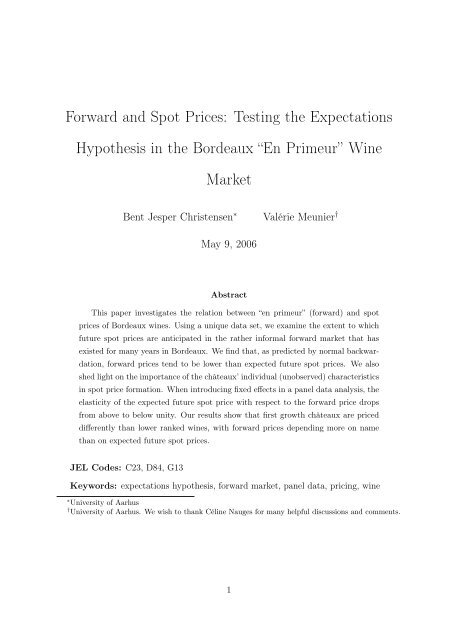
departure from this pattern in results concerns the rank 1 (highest quality) wines. Given 

the high value of the intercept (about 5), the low value of the slope (.26), the small portion 

of the variation explained (adjusted R 2 of only 5%), and the unrealistically low expected 

return (only 1%), we can outright reject every part of the theory for the topmost wines. A 

look at Figure 2 explains it all. Apart from chateau Ausone, all other first-rank wines set 

an identical forward price every year. This phenomenon may be traced back for at least 

the past 25 years. Nevertheless, the spot prices of these wines are not identical. What 

the regression shows is that the forward price is totally useless as a forecast of future spot 

prices for the top wines. 

To examine the robustness of our results, we consider in Table 4 the similar analysis, 

but using only the first spot price observed for each wine. The results are qualitatively 

similar. Slopes are slightly higher and expected returns slightly lower. Intercepts are now 

negative throughout, except for rank 1 wines. The theory is broadly confirmed for all 

subsamples except the top wines, for which again the slope is low, both statistically and 

economically, at .6, and significantly below unity at standard levels, and the intercept 

very high (in excess of 3). Thus, results using first spot price only confirm those using all 

spot prices, and we restrict attention to first spot prices in the remainder of the paper. 

Indeed, one characteristic of the Bordeaux en primeur market is that producers deliver 

the wine contracted upon to wholesalers as soon as it is bottled. It is thus the first spot 

price that should be the most relevant to traders. 

13

The poor forecasting power of the forward price relative to future spot prices of top 

wines suggests a possible market imperfection. Combined with the observation of identical 

forward prices across producers, it brings to mind the possibility of collusion. However, 

from the results, the forward price paid to producers systematically undervalues the top 

wines. This is clear both from the low slope and the very high constant term. 

In sum, our findings suggest that the en primeur market behaves quite similarly to a 

standard forward market, except for the top wines, where a very peculiar price-setting by 

producers takes place, albeit without any clear indication of harmful collusion. 

5 Conditional tests 

In a very simple regression like in (7), we do not capture everything. Several other factors 

may influence a wine’s spot price, particularly those related to information consumers rely 

on when purchasing wine. In the following, we introduce such variables in the analysis. 

As shown in different studies, consumers’ demand is driven by several of the wines’ at- 

tributes: blends of grapes, geographical origins, ranking, vintage,... (see Combris, Lecoq 

and Visser (1997)). In regressions in this section, we control for these attributes. More 

specifically, we account for the effect of the different vintages, ranks, and appellations. 

This yields a conditional test of the underlying theory. Given the rather strict definition 

of an official appellation (Appellation d’Origine Controlée, or Controlled Designation of 

Origin), the variable Appellation implicitly contains the information on grape varieties 

blending. Table 5 shows the results of the regression specification 

log SiT = α + β log fit + 

8 

k=1 

γkAik + 

4 

l=1 

δlRil + 

98 

m=94 

ηmVim + εiT 

where Aik and Ril are chateau-specific dummy variables for the appellation (area of pro- 

duction) and the rank, and Vim are dummy variables for the individual vintages. Thus, 

14 

(8)

Aik = 1 if wine i is produced in area k, 0 otherwise, Ril = 1 if wine i is classified as rank l, 

and Vim = 1 if wine i is of vintage m. 

Results are shown in Tables 5. In the first column, only vintage dummies are included. 

In the second, only rank dummies, and only appellation dummies in the third. Results in 

the fourth column are for the full specification including all three sets of dummy variables. 

Across the table, slopes on forward price are similar, slightly above unity, expected returns 

are all between 2% and 3% and significant, and intercepts negative, consistent with theory. 

All vintage dummies are significant, showing that later vintages differ from vintage 1994, 

the left out control group. In particular, the effect on spot prices is positive for vintages 

1995 and 1996, and negative for 1997 and 1998, relative to 1994. These findings are 

common across columns one and four, i.e., results do not depend on whether rank and 

appellation effects are included or not. As for rank, the results that stands out is that the 

top wines (rank 1) lie significantly above the remaining regression specification, i.e., the 

relevant dummy variable gets a high coefficient, at .27, and a t-statistic exceeding 4. The 

control group is rank 4, and there is no significant effect of being rank 2, whether vintage 

and appellation are included or not. In the full regression, last column, the effect of rank 

3 is insignificant, too, whereas this variable gets an apparently perverse negative sign 

in the specification with only rank dummies (the control group consists of non-classified 

wines). As for appellations, it turns out that only Pomerol is significant. It gets a positive 

sign (the control group is Saint-Julien), with a t-statistic of 2.60 in the full model, and 

the point estimate (.11) is the highest among all appellations. It is striking that exactly 

Pomerol, which is left out of the three classification systems, evidently carries high spot 

prices. Furthermore, this observation may be used to explain the apparently perverse 

sign on rank 3 in column 2. Thus, being unclassified, Pomerol wines belong to the control 

group in column 2, which focusses on ranks, but as Pomerol wines are pricey, they drive 

up the average price in rank 4, and the relative effect of rank 3 is estimated to be negative. 

However, when controlling for appellation (last column of the table), Pomerol gets the 

high positive coefficient, and the effect of rank 3 (relative to rank 4) vanishes. 

15

Overall, the results of this section confirm those obtained earlier. Slope on forward 

price, intercept and expected return are broadly consistent with theory, whereas rank 1 

(the highest quality) wines behave differently. In addition, we find that vintage has 

incremental explanatory power for spot price, and Pomerol wines carry high prices, but 

other appellation effects are already incorporated in the en primeur price. 

6 Panel data analysis 

In this section, we exploit the panel structure of our data set. The unit we consider is 

now a château, for which we have observations over several vintages (namely 5, from 1994 

to 1998). Furthermore, we are now explicitly only interested in the relation between the 

forward price of a château (fi) and its first spot price (S 1 i ). We therefore specify the 

following regression for château i: 

log S 1 iτ = c + β log fiτ + θi + eiτ, (9) 

for τ = 1994, ..., 1998. The forward price is indeed the only variable in our data set that 

varies across time and units. The other variables, as the rank or the appellation of a wine, 

are fixed across time and individuals. The term θi is the individual, unobserved effect of 

a wine i, and the error term eiτ is iid with zero mean. 

The individual, unobserved effect of a wine is likely to be correlated with the forward 

price set by the château. For instance, such an unobserved effect may contain a château’s 

reputation, or a specific technology, and will affect the way the forward price is fixed. We 

will thus conduct a fixed effect estimation of (9). 

Table 6 shows the results of the panel estimation. The fixed effects estimation proce- 

dure involves taking first differences. Hence, elapsed time is not included, but the time 

effect is captured by the constant term, which therefore has a different interpretation from 

the intercepts in earlier specifications and should not be negative. Variables constant in 

16

time, such as rank and appellation, also drop out when taking first differences. Vintage 

is not an explanatory variable, since it is used to form the groups of the panel. 

The first column of Table 6 shows the results for the basic specification with common 

slope β across all wines. This is now estimated at .77, and significantly below unity. This 

suggests that the findings from earlier sections of a slope above unity is not general. The 

inclusion of château-specific fixed effects allows for differences between châteaux unrelated 

to differences in forward prices, and when forward prices are only used to explain the 

remaining variation in spot prices after removing fixed effects, the coefficient drops. We 

believe the panel estimation is probably most relevant, i.e., we place more faith in the 

estimate of .77 than in the earlier estimates above unity. Indeed, the Hausman-Wu test 

is significant at the 1% level, showing that overall, the fixed effects are significant, and 

the panel approach most appropriate. More generally, the results show that, depending 

on specification, we can get slopes on forward prices above and below unity, showing that 

the average departure from expectations pricing is not that marked. 

Results for the case with a separate slope coefficient for each rank are shown in the 

second column of Table 6. Here, ranks 1 and 4, i.e., first growth and the unclassified wines 

including Pomerol, get lower coefficients, .66 and .68, than rank 2 and 3 wines, which get 

.82 and .81, respectively. Clearly, the coefficients on ranks 1 and 4 are nearly identical, 

and so are the coefficients on ranks 2 and 3. Wald tests confirm that the differences are 

insignificant at conventional levels. When re-estimating the model with equal coefficients 

for the two pairs of ranks, β is estimated at .67 for ranks 1 and 4, and at .81 for ranks 2 

and 3, with standard errors of .05 and .03, respectively, and the Wald test for equality 

of these two coefficients takes the value 5.21, for a p-value of 2.3% in the asymptotic χ- 

square distribution, significant at the 5% level. Evidently, pricing in the forward markets 

for rank 2 and 3 wines is not far from being consistent with the expectations hypothesis, 

whereas rank 1 and 4 wines (first growth and unclassified, including Pomerol) are priced 

are priced differently. 

17

The third column of Table 6 shows results with a separate slope for each appellation. 

Consistent with the results for separate rank (second column), Pomerol comes out as the 

appellation with the lowest coefficient, estimated at a mere .55. As the only appellation, 

Haut-Médoc has a point estimate in excess of unity, and the difference is insignificant. The 

remaining six appellations have slopes between .73 and .86, and the Wald test for equality 

of these does not reject at conventional levels. The model with equal coefficients for all 

appellations except Haut-Médoc and Pomerol produces an estimate of .79, with estimated 

standard error of .05, and the Wald test that this equals the Pomerol coefficient gets a 

p-value of 1.0%, clearly significant. This confirms that some wines are priced differently 

in the forward market, including the Pomerol. 

Table 6 also shows the standard errors of the estimated fixed effects θi and the error 

terms eiτ. The residual standard error σe is constant (.19 throughout), whereas the 

variation in fixed effects across châteaux σθ and hence the portion ρ of total error variance 

explained by this increases with the number of explanatory variables. With ρ of two- 

thirds or higher, the fixed effects approach appears quite successful in the application. 

Also reported are within, between, and overall adjusted R-squared statistics. The fixed 

effects estimator maximizes within-R 2 , which turns out to be nearly constant throughout, 

at about .57, suggesting that the basic specification with common slope at .77 is not bad, 

after all, and this impression is confirmed by the drop in adjusted (for degrees of freedom) 

R-square as regressors are added. 

To further investigate the nature of the estimated château-specific fixed effects, we 

finally regress these on rank and appellation. The results appear in Table 7. The three 

columns correspond to the three specification from Table 6. The results show that 42% 

or more of the variation in fixed effects may be explained by rank and appellation. This 

strong correlation rules out using alternative random effects estimators, which assume 

independence between château-specific effects and errors. The results show that rank 1 

and Pomerol wines on average have very high fixed effects. The result is also significant 

for Haut-Médoc, which gets a significantly negative effect, consistent with the higher 

18

slope from the previous table. Point estimates of average fixed effects are increasing by 

rank (rank 4 is the left out category) in the first column. The same applies for the third 

column, and to a lesser extent for the second column (the difference between ranks 2 

and 3 is insignificant), where fixed effects are from a model involving separate slopes by 

rank. Similarly, the third column results on appellation generally confirm the pattern 

from the first two columns, in particular the strong positive effect of Pomerol, but deviate 

somewhat from these, since fixed effects are from a model involving separate slopes by 

appellation. 

Overall, the change in results after introducing fixed effects in a panel analysis frame- 

work underscores the importance of the identity of the château in pricing in the forward 

market. Consistent with the results from earlier sections, the additional examination of 

the estimated fixed effects suggests that particularly first growth châteaux are priced dif- 

ferently. The forward prices of these wines depend less on expected future spot prices 

than for lower ranked wines. 

7 Conclusion 

In this paper, we have examined the extent to which prices in the informal forward market 

for wines that has existed for many years in Bordeaux reflect expected future spot prices. 

Depending on method used, we find elasticities of spot with respect to forward prices both 

above and below unity, broadly consistent with a version of the classical expectations 

hypothesis. However, when including relevant objective characteristics (vintage, rank, 

appellation, see e.g. Combris et al. (1997)), our results reveal important systematic 

departures from a pure expectations relation. Particularly forward prices of first growth 

châteaux depend more on name than on expected future spot prices. Our findings are 

consistent with a curious “reverse collusion” mechanism, by which producers meet early 

and fix a common price for first growth wines in the informal forward market which 

is actually on the low side, relative to rational expectations of subsequent spot market 

19

prices. Coordination of prices per se is consistent with standard collusion motives, given in 

particular that these well-known châteaux have a monopoly on famous names of Bordeaux 

wines. Whether avoiding competition between these famous names in order to protect 

reputation is truly sufficiently valuable to induce the setting of a common low forward 

price remains somewhat of a puzzle, which should be of interest for future research. 

20

References 

Anderson, R.W. (ed.) (1984). The Industrial Organization of Futures Markets. Lexing- 

ton, Massachusetts: D.C. Health and Company. 

Chang, E. C. (1985). “Returns to speculators and the theory of normal backwardation.” 

Journal of Finance, Vol. 40 (1985), pp. 193-208. 

Combris, P., Lecoq, S. and Visser, M. (1997). “Estimation of a hedonic price equa- 

tion for Bordeaux wine: Does quality matter?” Economic Journal , Vol. 107, pp. 390- 

402. 

Duffie, D. (1989). Futures Markets. Englewood Cliffs, New Jersey: Prentice-Hall. 

Hadj Ali, H. and Nauges, C. (2003). “Vente en primeur et investissement: Une etude 

sur les grands crus de Bordeaux.” Economie et Prevision, No. 159, pp. 93-103. 

(2006). “The pricing of experience goods: The case of en primeur wine.” Amer- 

ican Journal of Agricultural Economics, forthcoming. 

Houthakker, H. S. (1957). “Can speculators forecast prices?” Review of Economics 

and Statistics , Vol. 39, pp. 143-151. 

Keynes, J. M. (1930). A Treatise on Money. London: Macmillan. 

Mahenc, P. and Meunier, V. (2006). “Early sales of Bordeaux grands crus.” Journal 

of Wine Economics, forthcoming. 

21

Table 2: Summary statistics. 

Forward price First spot price Spot price Time 

Full Sample N 7099 698 7099 7099 

By Vintage 

Mean 86.03 137.03 172.76 9.32 

Sd 66.01 148.51 183.63 4.92 

1994 N 2057 136 2057 2057 

Mean 62.23 94.99 151.60 12.90 

Sd 34.06 80.86 126.86 4.84 

1995 N 2204 148 2204 2204 

Mean 75.22 118.86 194.73 9.31 

Sd 45.49 121.85 225.29 4.83 

1996 N 1592 151 1592 1592 

Mean 102.90 177.87 187.66 7.66 

Sd 72.69 204.52 202.30 3.44 

1997 N 925 146 925 925 

Mean 126.51 146.49 148.46 6.08 

Sd 101.04 142.01 138.49 2.01 

1998 N 321 117 321 321 

By rank 

Mean 112.39 144.36 153.56 4.05 

Sd 88.84 148.24 164.03 0.81 

Rank 1 N 386 34 386 386 

Mean 258.11 595.28 764.22 9.33 

Sd 103.82 251.26 278.64 5.04 

Rank 2 N 2687 249 2687 2687 

22 

Continued on next page


Mean 81.50 125.59 156.73 9.25 

Sd 45.58 89.08 95.74 5.00 

Rank 3 N 2378 242 2378 2378 

Mean 69.25 95.93 113.74 9.24 

Sd 39.86 63.95 64.71 4.93 

Rank 4 N 1648 173 1648 1648 

By Appellation 

Mean 77.29 120.93 145.52 9.56 

Sd 55.84 125.53 134.20 4.73 

HM N 722 78 722 722 

Mean 39.61 51.86 65.96 9.00 

Sd 13.48 25.09 31.35 4.81 

MA N 860 86 860 860 

Mean 75.09 119.88 169.34 9.11 

Sd 53.05 153.10 216.45 4.99 

PA N 1254 116 1254 1254 

Mean 92.48 164.91 217.98 9.44 

Sd 74.42 184.97 236.47 5.02 

PL N 843 85 843 843 

Mean 95.68 143.35 171.60 9.28 

Sd 66.98 142.81 158.19 4.87 

POM N 66 59 660 660 

Mean 111.01 204.59 220.99 9.19 

Sd 71.43 179.19 177.29 4.74 

23 

Continued on next page


SEGC N 1483 148 1483 1483 

Mean 98.99 151.74 185.36 9.28 

Sd 76.86 158.42 200.43 4.92 

SES N 554 52 554 554 

Mean 73.05 110.07 140.82 9.61 

Sd 41.61 69.15 84.34 4.94 

SJ N 723 74 723 723 

Mean 83.48 131.42 160.99 9.71 

Sd 53.09 108.74 116.75 4.94 

24

Price (FFR/bottle) 

300 

250 

200 

150 

100 

50 

0 

1996- 

Q3 

1996- 

Q4 

1997- 

Q1 

1997- 

Q2 

1997- 

Q3 

1997- 

Q4 

1998- 

Q1 

1998- 

Q2 

1998- 

Q3 

Time 

1998- 

Q4 

1999- 

Q1 

1999- 

Q2 

1999- 

Q3 

1992 1993 1994 1995 1996 1997 

Figure 1: Average spot prices. 

25 

1999- 

Q4 

2000- 

Q1 

2000- 

Q2 

2000- 

Q3

Table 3: Regression of (log) spot price on (log) forward price and time elapsed T − t. 

Sample Intercept (α) Slope (β) k Adj. R 2 Nb. Obs 

All (red) wines 0.479 1.024 0.68 7099 

(0.036)** (0.008)** 

All (red) wines -0.251 1.098 0.045 0.77 7099 

(0.033)** (0.007)** (0.001)** 

Vintage 94 -0.881 1.287 0.038 0.82 2057 

(0.059)** (0.014)** (0.001)** 


(0.056) (0.014)** (0.001)** 


(0.056) (0.012)** (0.002) 

Vintage 97 0.036 1.030 -0.008 0.98 925 

(0.023) (0.005)** (0.001)** 


(0.057)** (0.010)** (0.008)* 

Rank 1 5.014 0.264 0.012 0.05 386 

(0.330)** (0.057)** (0.004)** 

Rank 2 0.661 0.895 0.045 0.62 2687 

(0.065)** (0.014)** (0.001)** 

Rank 3 0.328 0.952 0.038 

(0.048)** (0.011)** (0.001)** 0.77 2378 

Rank 4 -0.057 1.050 0.041 

(0.071) (0.016)** (0.002)** 0.74 1648 

Standard errors in parentheses: * significant at 5% level; ** significant at 1% level. 

26

Table 4: Regression of first (log) spot price on (log) forward price and time elapsed T − t. 

Sample Intercept (α) Slope (β) k Adj. R 2 Nb. Obs 

All (red) wines -0.243 1.122 0.87 698 

(0.071)** (0.016)** 

All (red) wines -0.389 1.139 0.021 0.88 698 

(0.075)** (0.016)** (0.004)** 


(0.194)** (0.045)** (0.010)** 


(0.174)** (0.041)** (0.007)** 

Vintage 96 -0.593 1.237 -0.013 0.88 151 

(0.174)** (0.038)** (0.009) 

Vintage 97 -0.011 1.040 -0.006 0.99 146 

(0.058) (0.011)** (0.005) 


(0.103)** (0.016)** (0.018) 

Rank 1 3.190 0.598 -0.091 0.48 34 

(0.771)** (0.131)** (0.038)* 

Rank 2 -0.037 1.059 0.020 0.83 249 

(0.142) (0.031)** (0.008)* 

Rank 3 -0.031 1.048 0.016 0.89 242 

(0.102) (0.023)** (0.005)** 

Rank 4 -0.487 1.159 0.029 0.82 173 

(0.186)** (0.042)** (0.009)** 


27

Price (in Euro/bottle) 

600 

500 

400 

300 

200 

100 

0 

En Primeur Prices for Rank 1 wines 

92 93 94 95 96 97 98 

Vintages 

Ausone Cheval Blanc Haut-Brion Lafite-R Latour Margaux Mouton-R 

Figure 2: “En primeur” prices of Rank 1 wines 

28

Table 5: Regression of First (log) spot price on (log) forward price and time elapsed T −t. 

(1) (2) (3) (4) 

logprice logprice logprice logprice 

time 0.026 0.020 0.022 0.029 

(0.004)** (0.004)** (0.004)** (0.004)** 

logfwd 1.193 1.074 1.139 1.136 

(0.015)** (0.019)** (0.018)** (0.022)** 

i95 0.051 0.072 

(0.029) (0.029)* 

i96 0.077 0.110 

(0.028)** (0.029)** 

i97 -0.233 -0.193 

(0.028)** (0.029)** 

i98 -0.163 -0.124 

(0.029)** (0.030)** 

irank1 0.288 0.274 

(0.052)** (0.055)** 

irank2 -0.010 0.038 

(0.024) (0.027) 

irank3 -0.063 0.017 

(0.024)** (0.026) 

iHM 0.000 0.017 

(0.042) (0.038) 

iMA 0.022 0.013 

(0.039) (0.034) 

iPA 0.027 0.007 

(0.036) (0.032) 

iPL -0.057 -0.047 

(0.039) (0.036) 

iPOM 0.086 0.112 

(0.043)* (0.043)** 

iSEGC -0.036 -0.037 

(0.035) (0.032) 

iSES 0.015 0.023 

(0.044) (0.038) 

Constant -0.593 -0.091 -0.393 -0.417 

(0.070)** (0.084) (0.089)** (0.097)** 

Observations 698 698 698 698 

Adjusted R-squared 0.91 0.88 0.88 0.91 


29

Table 6: Panel data analysis. 

(1) (2) (3) 

logprice logprice logprice 

Constant 1.29** 1.27** 1.16** 

(.12) (.13) (.14) 

Logfwd .77** 

(.03) 

By rank 

Logfwd*rank1 .66** 

(.09) 


(.04) 


(.05) 


(.06) 

By appellation 

Logfwd*HM 1.12 

(.16) 

Logfwd*MA .77* 

(.10) 

Logfwd*PA .81** 

(.07) 

Logfwd*PL .86 

(.09) 

Logfwd*POM .55** 

(.08) 

Logfwd*SEGC .78** 

(.05) 

Logfwd*SES .73* 

(.10) 

Logfwd*SJ .74** 

(.08) 

σθ .27 .45 .70 

σe .19 .19 .19 

ρ .67 .84 .93 

R 2 : within .56 .57 .57 

Between .94 .51 .10 

overall .87 .52 .16 


30

Table 7: Analysis of predicted fixed effects. 

(1) (2) (3) 

θi θi θi 

Constant -.05 .31** .23** 

(.06) (.06) (.06) 

Irank1 .78** 1.02** .72** 

(.09) (.09) (.09) 

Irank2 .12* -.46** .1’ 

(.05) (.05) (.05) 

Irank3 .01 -.49** -.003 

(.05) (.05) (.05) 

Irank4 . . . 

iHM -.23** -.23** -1.66** 

(.07) (.07) (.07) 

iMA -.09 -.08 -.22** 

(.07) (.07) (.07) 

iPA -.06 -.05 -.36** 

(.06) (.07) (.07) 

iPL -.03 -.03 -.59** 

(.07) (.08) (.08) 

iPOM .24** .30** 1.1** 

(.08) (.08) (.08) 

iSEGC -.01 -.01 -.21** 

(.06) (.06) (.07) 

iSES -.03 -.02 -.01 

(.08) (.08) (.08) 

iSJ . . . 

Adj. R 2 .42 .77 .90 


31

Forward and Spot Prices: Testing the Expectations Hypothesis in the ...

Create successful ePaper yourself

Delete template?

Save as template?