Motivational Goal Bracketing - School of Economics and ...

Motivational Goal Bracketing
Alexander K. Koch a and Julia Nafziger b∗
a Aarhus University and IZA
b Aarhus University
October 2, 2009
Abstract
It is a puzzle why people often evaluate consequences of choices separately (narrow
bracketing) rather than jointly (broad bracketing). We study the hypothesis that a
present-biased individual, who faces two tasks, may bracket his goals narrowly for mo-
tivational reasons. Goals motivate because they serve as reference points that make
substandard performance psychologically painful. A broad goal allows high perfor-
mance in one task to compensate for low performance in the other. This partially
insures against the risk of falling short of ones’ goal(s), but creates incentives to shirk
in one of the tasks. Narrow goals have a stronger motivational force and thus can
be optimal. In particular, if one task outcome becomes known before working on the
second task, narrow bracketing is always optimal.
JEL Classification: A12, C70, D91
Keywords: Goals; Multiple tasks; Motivational bracketing; Self-control; Time incon-
sistency; Psychology.
∗ We thank Johannes Abeler, Juan Carrillo, Georg Nöldeke, Hideo Owan, Heiner Schumacher, Frederic
Warzynski, and Yoram Weiss for helpful comments and discussions. Contact: School of Economics and
Management, Aarhus University, Building 1322, 8000 Aarhus C, Denmark. a Email: akoch@econ.au.dk, Tel.:
+45 8942 2137. b Email: jnafziger@econ.au.dk, Tel.: +45 8942 2048.
1

1 Introduction
People often evaluate consequences of choices separately (narrow bracketing) rather than
jointly (broad bracketing). 1 For example, a student might set himself the narrow goals
to “achieve a score of 60% in each exam this term”, rather than the broad goal to “get an
average score of 60% over all exams this term”. Such narrow goals however seem at odds with
maximizing behavior, as Read et al. (1999, p.171) note: “Because broad bracketing allows
people to take into account all the consequences of their actions, it generally leads to choices
that yield higher utility.” We investigate one possible explanation for this puzzle: people
bracket their goals narrowly for motivational reasons, to overcome self-control problems – a
process for which Read et al. coined the term motivational bracketing (see also Thaler and
Shefrin 1981, Kahneman and Lovallo 1993).
As an illustration of how important motivational goal bracketing may be for everyday eco-
nomic decisions, consider the study of New York City cab drivers’ labor supply behavior by
Camerer et al. (1997). The cab drivers appear to set a daily income goal for themselves,
choose their working hours accordingly, and therefore display a negative wage elasticity. 2
Yet by taking it “one day at a time”, they forgo gains in earnings and leisure that they
could realize, for example, with a weekly target. Such a broader target would allow them to
work fewer hours on days with low wages by compensating with more hours on days with
high wages. The reason that cab drivers nevertheless set daily income targets is that narrow
goals may be better at mitigating self-control problems than a broad goal, as Camerer et al.
(1997, p.427) as well as Read et al. conjecture: “If [cab drivers] had, for example, picked
a weekly target they might have been tempted to quit early on any given day, while assuring
themselves that they could make up the deficiency later in the week” (Read et al. 1999, p.189).
Correspondingly, our model of goal bracketing is built around a self-control problem that
arises from a present bias (e.g., Strotz 1955, Phelps and Pollak 1968, Ainslie and Haslam
1992, Laibson 1997, O’Donoghue and Rabin 1999). For instance, an individual may judge
that going for morning runs is in his long-run interest. But come the start of a day, the
distant health benefits suddenly do not seem worth the effort. The preference reversal occurs
because the costs become more salient when they are immediate and loom larger than the
gains, which only accrue in the future.
Personal goals play an important role in helping to overcome such motivational problems.
1 The terms go back to Read et al. 1999. The phenomenon is also referred to as narrow framing
(Kahneman and Lovallo 1993), or mental accounting (Thaler 1980, 1985, 1990, 1999).
2 Camerer et al. (1997) triggered a lively debate about the estimation of wage elasticities of labor supply
(see Goette et al. 2004; Farber 2005, 2008; Fehr and Götte 2007; Crawford and Meng 2008). Particularly
relevant for our purposes is the link between loss aversion and effort elasticities suggested by Fehr and Götte’s
(2007) field experiment (see Footnote 6).
2

Bandura, for example, writes that “the regulation of motivation by goal setting is a remark-
ably robust phenomenon” (p.xii of his foreword to Locke and Latham 1990a). Goals serve as
reference points against which actual task outcomes are measured, and people display loss
aversion regarding goal achievement. 3 Falling short of a goal hence causes a psychological
loss that weighs more heavily than the gain from achieving the goal. A consequence is that
a higher goal raises the motivation of a future self to work hard. Yet a higher goal also
increases the chances of falling short of the performance standard and thereby suffering a
loss. So goals are painful self-disciplining devices; and this limits their attraction for self-
regulation (see also Koch and Nafziger 2008). The key question we address is how people
use goals when they face multiple tasks. Does an individual prefer to set narrow goals (i.e.,
to measure each task outcome against a separate performance standard) or a broad goal
(i.e., to evaluate the combined task outcomes against a global performance standard)? Our
model sheds light on the puzzle why people often bracket narrowly by making clearer the
trade-offs involved, and yields conditions under which narrow bracketing is indeed optimal.
Our analysis starts by looking at the case where an individual works sequentially on two
independent tasks, but does not learn about the outcome of the first task before deciding
how much effort to put into the second task (the no-information scenario). We then turn to
the case where the individual receives intermediate information (the information scenario).
Intuitively, in the no-information scenario, a broad goal seems appealing because it pools
outcomes across tasks and thus provides a partial hedge against the risk of falling short of
the goal despite best efforts: a high outcome in one task can compensate for a low outcome
in the other task. In contrast, with narrow goals the individual suffers a psychological loss
in a task as soon as the respective task outcome is low. Due to this risk-pooling effect, the
expected psychological cost of using a broad goal is lower than that for corresponding narrow
goals.
The possibility of compensating for low performance in one task with high performance in
the other task however also makes it more attractive to “lean back”: if the individual shirks
in one of the tasks, he can still achieve the broad goal and avoid a psychological loss. But the
3 Summarizing decades of psychology research on goals, Locke and Latham write that “goals serve as the
inflection point or reference standard for satisfaction versus dissatisfaction [...] For any given trial, exceeding
the goal provides increasing satisfaction as the positive discrepancy grows, and not reaching the goal creates
increasing dissatisfaction as the negative discrepancy grows” (Locke and Latham 2002, p.709-710). For an
extensive survey see Locke and Latham (1990a). Heath, Larrick, and Wu (1999) note the similarity to the
value function in Kahneman and Tversky’s (1979) Prospect Theory, and present evidence supporting the
view that goals work in conjunction with loss aversion. Using a controlled lab experiment to manipulate
subjects’ reference points, Abeler et al. (2009) observe that higher reference levels induce higher effort.
3

fear of facing such a loss when shirking is where the incentive effect of a goal stems from. 4 So
a broad goal provides lower motivation for working hard in both tasks than corresponding
narrow goals. What our model shows, however, is that the leaning-back effect alone is not
sufficient for narrow goals to be optimal: there still are cases where the risk-pooling effect
dominates, so that a broad goal performs better than narrow goals.
An additional effect arises if the individual receives intermediate information between the
tasks – a setting that seems particularly relevant for many applications. For instance, the
two different tasks may correspond to two working days of a cab driver in Camerer et al.
(1997), where a driver knows what he earned on the previous day.
Again, a broad goal allows for low performance in one task to be offset by high performance in
the other task, giving rise to the leaning-back effect. But, because the individual can observe
the outcome of the first task before working on the second task, a second effect arises that
further undermines the motivating force of a broad goal. If the individual observes that he
was successful in the first task and has already achieved his goal, he will “rest on his laurels”
and put in low effort in the second task. In contrast, if he observes a failure in the first task,
he will work hard in the second task to still meet the goal. This asymmetric response, in
turn, exacerbates the temptation to shirk in the first task. The reason is that the individual
wants his future self to work hard and not to rest on his laurels. But hard work today, in
addition to being painful, makes it more likely that the future self will rest on his laurels;
so the individual is tempted not to give his best today. To overcome this temptation, the
broad goal has to be much higher than what would be needed if the individual received
no intermediate information. As we show, the resting-on-your-laurels effect and its adverse
impact on first-period incentives make the broad goal perform worse than narrow goals: in
the information scenario, narrow bracketing is always optimal.
Overall, our model helps clarify the driving forces for narrow goal bracketing. The leaning-
back effect for example captures what Camerer et al. (1997, p.427) might have had in mind
in their discussion of why cab drivers set a daily income target: “A weekly or monthly target
[instead of a daily one] would leave open the temptation to make up for today’s shortfall to-
morrow, or next week, and so on”. While intuitively appealing as an explanation for narrow
goals, our analysis shows that this effect on its own is not necessarily enough to overcome
the disadvantages of narrow bracketing. Rather, our model suggests that intermediate in-
formation between the tasks, and the resulting resting-on-your-laurels effect and its adverse
impact on first-period incentives, play a crucial role in explaining many of the instances of
narrow goal bracketing that we observe.
The paper is organized as follows. Next, we discuss the related literature. Section 2 then
4 In line with this, Heath, Larrick, and Wu (1999) observe that workers are twice as willing to provide
effort to just meet a given goal than they are willing to work toward surpassing the goal.
4

introduces our model of goal setting in a multiple-task environment, which is based on the
single-task model in Koch and Nafziger (2008). To obtain closed-form solutions we simplify
that model by using a binary variable to describe task outcomes. While this simplification
makes the model tractable, none of its essential properties are lost, as we discuss in Section
3. This section also prepares the analysis of the no-information and information scenarios,
which follow in Sections 4 and 5, respectively. Section 6 concludes the paper.
Related Literature
Our paper contributes to three literature strands. First, the research on goals, carried out
mainly by psychologists (for an overview see e.g. Locke and Latham 1990a). Most of these
studies investigate the effect of given goals (e.g., exogenously assigned by an experimenter)
on incentives and performance in various tasks. 5 We analyze how individuals choose and
design goals for themselves, thereby filling this gap and contributing to the small economics
literature on goal choice (Falk and Knell 2004, Koch and Nafziger 2008, and in parallel and
independent work to our papers, Suvorov and van de Ven 2008 and Hsiaw 2009a, 2009b).
Our multiple-task model of goal setting is based on the single-task framework in Koch and
Nafziger (2008), which is complementary to the single-task models by Suvorov and van de
Ven (2008) and Hsiaw (2009a). They take a different approach and model goals as self-
fulfilling rational expectations. Most closely related to our question is Hsiaw (2009b), who
extends her single-task model to study goal bracketing with two sequential continuous-time
optimal stopping problems. In contrast to our model, costs and benefits from a project
accrue at the same time, and it is the tension between the option value of waiting versus
stopping today at a known project value that gives rise to a self-control problem. Goals
help counter the tendency of the present-biased individual to stop projects too early. So
the intuition is quite different from the one developed in our model. First, narrow goals
allow better regulation of stopping times relative to a broad goal, but cause disutility from
frequent goal evaluation. Second, as Hsiaw assumes that the agent receives no intermediate
information between the periods, the resting-on-your-laurels effect that arises in our model
plays no role in her results.
Falk and Knell’s (2004) social comparison model looks at the role of self-enhancement (people
use comparisons with others to make themselves feel better) and self-improvement (people
use comparisons with others to improve their own performance) for goal choice. We highlight
5 For example, Fuhrmann and Kuhl (1998, p.653) note: “Goals are typically considered to be ‘just there’
and the interest of research mostly remains restricted to the process of how the organism manages to reach
goals. We believe that the process by which goals are formed and become an object of self-regulation deserves
much more attention in self-regulation research.” Similarly, Bargh (1990), Carver and Scheier (1999), and
Oettingen, Pak, and Schnetter (2001) mention that little is known about why and how people set goals for
themselves.
5

another important motivation for goal setting: the regulation of own behavior when people
face self-control problems.
Second, our paper relates to the choice bracketing literature, that goes back to Tversky and
Kahneman (1981), Simonson (1990) and Herrnstein and Prelec (1991) (for an overview see
e.g. Read et al. 1999; Thaler 1999). Narrow bracketing is observed in a wide range of
settings, such as consumption decisions (Cicchetti and Dubin 1994, Heath and Soll 1996) or
lottery choices (Tversky and Kahneman 1981, Thaler, Tversky, Kahneman, and Schwartz
1997, Rabin and Weizsäcker 2009).
In conjunction with loss-aversion, a narrowly defined reference point can account for a
range of puzzles and “wrong” decisions, such as the equity premium puzzle (Benartzi and
Thaler 1995, Gneezy and Potters 1997), low stock market participation (Barberis 2001),
choice errors (Thaler 1999), asymmetric price elasticities (Hardie, Johnson, and Fader 1993),
the fact that investors hold on to “loosing” stocks too long (Odean 1998), and why workers
work fewer hours/provide less effort on high-wage days – as e.g., the cabbies in Camerer et
al.’s (1997) study, or the bicycle messengers in Fehr and Götte (2007). 6 The puzzle however
is that broad bracketing would (all else equal) lead to better outcomes than narrow brack-
eting.
Third, our paper contributes to the theoretical literature that deals with the question how
present-biased individuals cope with self-control problems (for an overview see e.g. Brocas,
Carrillo, and Dewatripont 2004). Much of this literature focuses on the role of external com-
mitment technologies for achieving pre-commitment (Elster 2000). Only a few contributions
deal with intra-personal strategies, as our paper. Similar to our approach, Benhabib and
Bisin (2005) and Herweg and Müller (2008) assume the presence of an internal commitment
device and ask how an individual can use it to regulate behavior. Koch and Nafziger (2009)
model the use of self-rewards. In a model where an individual has imperfect recall about past
motives, Bénabou and Tirole (2004) can explain why internal commitment devices actually
work.
2 The model
Overview. An individual needs to decide how much effort to put into two tasks that oc-
cur in sequence. In the no-information scenario, the individual does not learn about the
6 Camerer et al. (1997) observe that narrow bracketing and loss aversion relative to a reference point seem
to go hand in hand. Fehr and Götte’s (2007) field experiment is in line with a link between loss aversion and
narrow income targets. In response to an exogenous and transitory 25 percent increase in the commission
rate, bicycle messengers with higher loss aversion (elicited using lottery choices) displayed more negative
effort elasticities. Those with no loss aversion did not have a significantly negative elasticity.
6

outcome of the first task before working on the second task. In the information scenario,
the individual receives intermediate information before working on the next task. The cost
of effort for a task is immediate, whereas the task outcome (and the related utility) realize
only later. The individual has a present bias, and this bias creates an intra-personal conflict
of interest: before the individual faces the tasks he thinks that working hard in both tasks
is optimal; but once he makes the actual effort choices, all else equal, he will shirk. In antic-
ipation of this self-control problem, the individual sets goals that serve as reference points
for the future outcomes.
The tasks. The individual faces two symmetric tasks i ∈ {1, 2}. Each task leads to an
outcome yi ∈ {y, ¯y}, where ¯y > y. We normalize y ≡ 0. For each task the individual can
choose whether to work hard (ēi = 1) or shirk (e i = 0). Effort causes an instantaneous
utility cost c · ei. The outcome depends on both effort and luck: effort in task i leads to a
successful outcome yi = ¯y with probability p · ei, where p ∈ (0, 1). The outcome realization
for each task is independent of that in the other task.
Goal setting. Before working on the tasks, the individual can choose a goal which then
becomes anchored in his head as a standard for the future outcome to be achieved: he can
either specify a separate reference standard for each task i ∈ {1, 2}, i.e., a narrow goal
ani
∈ [0, ∞), or a global reference standard for the sum of the outcomes in both tasks, i.e., a
broad goal ab ∈ [0, ∞), or no goal (which corresponds to a reference standard that will be met
for sure, i.e., ani = 0 or ab = 0). 7 The assumption that an individual has the capacity to set
goals for himself that remain meaningful over time is grounded in the psychology literature.
For example, Gollwitzer (1999) writes: “By forming goal intentions, people translate their
noncommittal desires into binding goals. The consequence of having formed a goal intention
is a sense of commitment that obligates the individual to realize the goal.”
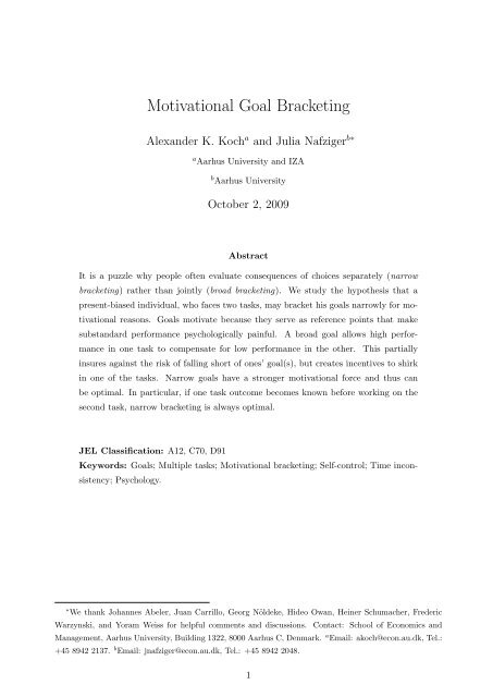
Timing and utilities. Figure 1 summarizes the timing. At date 0, the individual chooses
the goal bracket and level(s): a broad goal (ab), two narrow goals (an1, an2), or no goal. No
payoff-relevant events occur, so u0 = 0.
Date-1 utility reflects the immediate cost of effort exerted in the first task: u1 = −c(e1). At
date 2, the individual works on the second task, so u2 = −c(e2). In the information scenario,
he observes the outcome of task 1 before he provides effort at date 2. In the no-information
7 The lower bound on the goal level captures the idea that goals have to be “realistic” (e.g., Locke and
Latham 1990b): the individual cannot make himself infinitely happy by setting the goal “I want to achieve
−∞ points in the exam” even though the lowest possible outcome is zero points (as explained below, the
lower the goal, the better the individual feels about a given level of performance). Imposing a “realistic”
upper bound would not change any of our results: as we show, a narrow goal greater than ¯y, or a broad goal
greater than 2 ¯y, has no motivational power.
7

date 0 date 1 date 2 date 3
goal choice:
- broad goal
(ab)
- narrow goals
(an1, an2)
- no goal
effort choice
for task 1 (e1)
scenario, he does not observe it. 8
- effort choice
Figure 1: Timing
for task 2 (e2)
- info scenario:
outcome of
task 1 observed
- info scenario:
outcome of
task 2 observed
✲
- no-info scenario:
outcomes of
tasks 1 and 2
observed
- goals are
evaluated
At date 3, the individual experiences utility related to the realized task outcomes and the
goal(s). There is extensive psychological evidence that people experience a loss if they fall
short of a goal and a gain if they exceed it. Losses loom larger than gains of equal size.
For example, Bandura (1989, p.1180) summarizes that “people seek self-satisfactions from
fulfilling valued goals” and experience “discontent with substandard performances” (see also
Section 1). We capture this with a value function in the spirit of Kahneman and Tversky
(1979): depending on the difference between the outcome realization y and the goal a, the
individual experiences a gain µ + (y −a) from satisfying the goal if y ≥ a, and a loss µ − (a−y)
from falling short of the goal if y < a. 9 As in many applications of Kahneman and Tversky’s
(1979) gain-loss utility framework, we assume for tractability that the individual exhibits
linear loss aversion: µ + (y − a) = max{y − a, 0} and µ − (y − a) = µ · max{a − y, 0}, with
µ > 1.
With narrow goals ani , gain-loss utility relates to individual task performance yi, i = 1, 2:
u3 =
2
(max{yi − ani , 0} − µ max{ani − yi, 0}) .
i=1
And with a broad goal ab, the overall performance y1 + y2 is measured against the goal:
u3 = max{(y1 + y2) − ab, 0} − µ max{ab − (y1 + y2), 0}.
8 The no-information scenario yields the same results as a scenario where the individual works simultane-
ously on both tasks, as we show in Appendix B.
9 In a somewhat different context, Köszegi and Rabin (2006) refer to such a gain-loss utility function as
the individual’s “psychological utility”, which they distinguish from an outcome-based consumption utility
component. Making such a distinction, by adding a consumption utility component (say, v(y) = y), would
not change our qualitative results (but add notational clutter). With v(¯y) > v(y) ≥ 0, a high outcome is
more valuable relative to our setting. So the parameter range where a conflict of interest between self 0
and self 1 arises (Assumption 1) becomes smaller, but is still non-degenerate. Moreover, self 0 is willing to
specify a “painful” goal for a larger range of parameter values.
8

In the absence of a goal, simply set ab = 0 (or ani = 0).
Our setup is a simplified version of the single-task goal setting model in Koch and Nafziger
(2008). There, both the goal level and the outcome have the same continuous support, i.e.,
a goal always corresponds to a possible outcome level. The key property however is that
varying the goal level shifts the expected psychological gain from exceeding the goal relative
to the expected psychological loss from falling short of it. Our setting preserves this essential
feature, while making the model sufficiently tractable for analyzing multi-task problems (see
Section 3).
Present bias. The individual has time-inconsistent preferences in the sense of Strotz (1955).
A present bias causes current payoffs to be more salient than future payoffs. Following the
literature (e.g., Phelps and Pollak 1968, Laibson 1997, O’Donoghue and Rabin 1999), we
model this using (β, δ)-preferences. The first parameter, δ, corresponds to the standard
exponential discount factor (for simplicity, we assume δ = 1). The second parameter, β ∈
[0, 1), captures the extent of the present bias, and is the parameter of interest in our model.
The utility of the individual at date t ∈ {0, 1, 2, 3} is given by:
Ut =
3
ut + β
, (1)
τ=t+1
where ut is the instantaneous utility at date t. For instance, the date-0 incarnation of the
individual (self 0 ) weighs future utilities u1, u2 and u3 equally; but the date-1 incarnation
of the individual (self 1 ) puts a larger relative weight on u1 by discounting u2 and u3 with
β < 1, reflecting his present bias. We assume that self 0 knows about the present-biased
preferences of his future selves, i.e. is sophisticated in the sense of O’Donoghue and Rabin
(1999). Without this knowledge, self-regulation clearly would make no sense.
Self-control problem. To make the problem interesting, we assume that a conflict of
interest between self 0 and later-date selves arises in the absence of a positive goal level. For
self 0 the choice of effort still lies in the future, and he therefore weighs equally the effort
costs and the future benefits related to each task outcome. High effort in a task is therefore
optimal from the date-0 perspective if the expected utility it yields (β {p ¯y − c}) exceeds
that from low effort (β y = 0). That is, self 0 wants his future self to work hard in the tasks
if and only if
uτ
β { p ¯y − c} ≥ 0. (2)
Only in the case with no present bias (β = 1) does self 1 (or self 2) choose exactly as self
0 would. But because β < 1, the individual overemphasizes immediate costs relative to the
distant benefits. As a result, self 1 (self 2) may prefer to shirk, while self 0 wants his later
incarnation(s) to work hard. To see this formally, note that in the absence of a goal it is
9

optimal to provide low effort from the perspective of self 1 (self 2) if and only if
β p ¯y − c < 0, (3)
Thus, whenever both (2) and (3) hold, the individual has a self-control problem. The
following assumption summarizes this.
Assumption 1 (Self-control problem) Self 0 prefers high effort in each task, but in the
absence of a goal, the self making the effort decision on a task will choose low effort, i.e.,
p ¯y ≥ c and
βsc ≡ c
p ¯y
> β. (4)
3 The basics of goal setting (a single task)
To prepare for our main analysis, we first look at how an individual sets a goal for himself if
there is only a single task to be completed. When designing his task goal, self 0 anticipates
what it takes to motivate self 1 to provide effort. We therefore solve by backward induction:
starting with the effort choice at date 1, we ask how self 1 responds to a given goal. Then
we determine what is the optimal goal from the perspective of self 0.
3.1 The incentive effect of a given goal
For a given goal related to the task, self 1 provides high effort if and only if the expected
utility of self 1 if he works hard exceeds that if he shirks: U1(a; ē) ≥ U1(a; e). For a ≤ ¯y this
“incentive constraint” is given by (see Appendix A.1):
a β (µ − 1) [Pr(loss|e) − Pr(loss|ē)] ≥ c − β p ¯y, (5)
where Pr(loss|e) gives the probability that the individual falls short of the goal (thereby
suffering a psychological loss) when providing effort level e. The incentive constraint shows
how and why a goal motivates an individual to work hard. Think of studying for an exam.
Cramming yields self 1 net-utility β p ¯y − c, which however is negative: the benefit from
an expected good grade does not compensate for the cost of studying hard, because of the
individual’s present bias (Assumption 1). Hence, self 1 would refrain from working hard in
the absence of a goal. Motivating himself to study for an exam however is easier if he has a
target grade, as he then fears suffering a loss from not reaching his goal. If self 1 shirks, the
probability of failing the goal is larger (it is equal to 1) than if he works hard (the probability
then is 1 − p) – so the left-hand side of the incentive constraint is positive. Hence, with an
appropriately chosen goal, the loss avoided by exerting effort offsets the net cost from hard
work. More precisely, the goal level, where (5) just holds, is given by
â =
c − β p ¯y
. (6)
β p (µ − 1)
10

The more severe the present bias (i.e., the lower β), the more difficult it is to incentivize self
1 and thus the higher the required goal level â. If however the present bias is so strong that
â exceeds ¯y, self-regulation becomes impossible. The reason is that in this case the incentive
constraint (5) needs to be modified: with such a goal the individual experiences a loss no
matter whether he works hard or shirks. As loss aversion no longer kicks in, the goal simply
cancels out from the incentive constraint. 10 In sum, self-regulation with a goal is feasible if
and only if â ≤ ¯y, which is equivalent to 1
µ βsc ≤ β (βsc is defined in Assumption 1).
3.2 What goal does self 0 choose?
Holding the effort level e fixed, a higher goal increases the chance of falling short of the
aspired outcome a. But this matters more than the chance of exceeding a, because losses
loom larger than gains of equal size. So a higher goal level is painful, because it reduces the
utility self 0 expects from a given effort level e: d
d a U0(a; e) < 0.
This shows clearly that the only purpose of setting a > 0 is to discipline self 1 to put in
more effort than he would exert in the absence of a positive goal. Thus, the choice of self 0
is a relatively simple one: either avoid the pain from an ambitious goal by abstaining from
goal setting, and live with low effort; or pick the goal level that just suffices to motivate self
1 to work hard (if this is feasible). In other words, self 0 will specify a positive goal if his
expected utility with goal â and high effort in the future exceeds the utility from a = 0 and
low effort in the future: U0(â; ē) ≥ U0(0; e) = 0. Lemma 1 below characterizes this in terms
of β (it corresponds to Proposition 1 in Koch and Nafziger 2008).
4 Risk pooling vs leaning back (the no-information
scenario)
We start our analysis of the two-task setting with the no-information scenario, where the
individual does not learn about the first task outcome before working on the second task.
For example, think of studying for two exams in unrelated subjects, that take place in close
sequence. Before even taking the first exam, you need to already study for the second exam.
So all you know is how much (or little) effort you put into preparing for the first exam.
4.1 Self-regulation with narrow goals
If the individual sets narrow goals, he will evaluate task outcomes separately. (Did I reach
the target grade in the first exam? Did I in the second?) Given the symmetry of tasks, the
problem for each task hence mirrors the one in the single-task setting above. The minimum
10 −β µ {p (a − ¯y) + (1 − p) a} − c ≥ −β µ a. ⇔ β p ¯y ≥ c, which does not hold because of Assumption 1.
11

narrow goal level required to motivate self 1 to work hard on task i is just the one from
Equation (6), i.e.,
ân =
c − β p ¯y
. (7)
β p (µ − 1)
The following result provides the conditions under which self-regulation with narrow goals
is more attractive than no goal (i.e., when U0(ân, ân; ē1, ē2) ≥ U0(0, 0; e 1, e 2) = 0).
Lemma 1
(i) Self-regulation with narrow goals is feasible if and only if 1
µ βsc ≤ β.
(ii) There exists a cutoff βn, satisfying 1
µ βsc < βn < βsc, such that for β ∈ [βn, βsc) self 0
sets the narrow goal ân from (7) for each task rather than no goal, and self 1 and 2
provide high effort.
In other words, there exists a range for the present bias parameter β, for which self 0 would
find it worthwhile to engage in self-regulation with adequately chosen task-specific goals
(ani = ân). If there was no intra-personal conflict of interest – i.e., if β exceeded βsc – no
goal would be needed: self 1 would exert high effort anyway. In contrast, if β falls in between
1
µ βsc and βn, it would be feasible to overcome the self-control problem with narrow goals, yet
the required goal levels are too painful for self 0. So he rather gives up on self-regulation. If
the self-control problem is very severe, β < 1
µ βsc, no feasible narrow goal can help overcome
it (but by the previous argument, it would be too painful to do so anyhow).
4.2 Self-regulation with a broad goal
The alternative to narrow task-specific goals is to set a broad goal related to the overall
outcome from both tasks (e.g., reach some average grade score in the upcoming exams).
One needs to distinguish between two cases. Is an “easy” broad goal ab ≤ ¯y, that can be
achieved with one task outcome alone, enough to motivate self 1 and 2? Or does the goal
have to be more ambitious, i.e., ¯y < ab ≤ 2 ¯y (a “difficult” broad goal)? The difficult goal is
more painful, and therefore only makes sense if an easy broad goal does not do the job.
When does an easy broad goal make sense? 11 Because the individual evaluates the outcomes
of the two tasks jointly, the (previous or expected future) effort choice of the other self
influences the incentives of the current self. So we have to consider two cases: does the other
self work hard, or does he shirk? If there will be shirking in one task, say by self 1, the broad
goal necessary to motivate self 2 just equals the narrow goal for that task – i.e., ab = ân
from Equation (7). Yet if high effort in this task is worth the cost of the goal, then effort in
the other task is also worth it. So in this case, narrow goals (ân, ân) dominate.
11 Formal details for the following arguments are given in Appendix A.3.
12

Now consider what it takes to get both self 1 and 2 to put in effort. If self 2 knows that his
previous self worked hard at date 1, a broad goal ab ≤ ¯y provides incentives for him to work
hard in the second task if:
ab β (µ − 1) [Pr(loss|e 2, ē1) − Pr(loss|ē2, ē1)] ≥ c − β p ¯y. (8)
The interpretation is similar to that of the incentive constraint (5) for the single-task set-
ting/narrow goals: while shirking saves c − β p ¯y – the net-utility cost of effort of self 2 in
the task (note that the effort cost of self 1 is already sunk) – it exposes the individual to
the risk of falling short of the goal. Shirking now however does not for sure lead to a loss
(as under narrow goals), but only with probability 1 − p: a high outcome in the first task,
where self 1 put in effort already, can compensate for the low outcome that shirking causes
in the second task. By working hard, self 2 can reduce the probability of a loss to (1 − p) 2 .
So Pr(loss|e 2, ē1) − Pr(loss|ē2, ē1) = p (1 − p), and the broad goal necessary to motivate self
2 is given by:
âb =
c − β p ¯y
. (9)
β p (1 − p) (µ − 1)
This goal also motivates self 1 to work hard if he expects self 2 to put in effort. The reason
is that the incentive constraint of self 1 simply reduces to the one in (8): the anticipated
effort cost of self 2 appears on both sides of the incentive constraint, and thus cancels out
without influencing the decision of self 1 whether to work hard or shirk.
The following result provides the condition under which the “easy” broad goal âb ≤ ¯y is
better than abstaining from setting a positive goal altogether (i.e., when U0(âb; ē1, ē2) ≥
U0(0; e 1, e 2)).
Lemma 2
(i) Self-regulation for both tasks with an “easy” broad goal (¯y ≥ ab > 0) is feasible if and
only if
1
(1−p) µ+p βsc ≤ β.
1
(ii) There exists a cutoff βb satisfying (1−p) µ+p βsc < βb < βsc, such that for β ∈ [βb, βsc)
self 0 sets the “easy” broad goal âb from (9) rather than no goal, and self 1 and 2
provide high effort.
Similar to the case of narrow goals, even if a broad goal that would help overcome the self-
control problem is feasible, this does not mean that the individual is willing to use it. For
1
(1−p) µ+p βsc < β < βb, it is better to set no goal than to assure effort at the cost of a painful
broad goal.
This, as we now argue, also implies that a difficult broad goal (¯y < ab ≤ 2 ¯y) can never be
optimal. Self 0 will consider such a goal only if it is not possible to solve the motivation
problem with an easy broad goal. In the parameter range where this is true, β <
1
(1−p) µ+p βsc,
the benefit of higher effort however does not even outweigh the cost of setting an easy broad
13

goal. So, a fortiori, a difficult broad goal would yield negative utility for self 0. First, there
is a larger loss of falling short of the goal, as it is larger (by construction) than any easy
broad goal. Second, a high outcome in one task can no longer fully compensate for a low
outcome in the other task, so the individual also suffers a loss more often than with an easy
broad goal.
Lemma 3 Self 0 will never adopt a “difficult” broad goal (¯y < ab ≤ 2 ¯y).
As the easy broad goal âb is the only candidate that can beat narrow goal bracketing, we
will henceforth refer to the easy broad goal simply as the broad goal.
4.3 Motivational bracketing: broad vs narrow goals
Is broad or narrow goal bracketing better suited for self-regulation? To answer this question,
suppose first that those goals that motivate the individual – be they broad or narrow –
dominate setting no goal (i.e., β ≥ max{βn, βb}).
4.3.1 The risk-pooling effect
Broad bracketing would be superior if we were able to abstract from incentive considerations
(say, because self 1 always works hard), and simply compared the utility of self 0 in the
broad and narrow bracketing scenarios for the same goal level (say, a = ab = an). Under
both scenarios, the individual experiences disutility 2 c from working hard in the tasks, and
looks forward to an expected utility flow from the task outcomes of 2 p ¯y in the future. In
addition, he has to incur the psychological cost of goal setting. But that cost under broad
bracketing is different from the one under narrow bracketing: there is a risk-pooling effect.
Specifically, as the broad goal is lower than ¯y (Lemma 3), a high outcome in one task can
compensate for a low outcome in the other task. The individual therefore experiences a loss
only if the outcomes in both tasks are low, so the expected loss is (1 − p) 2 µ a. In contrast,
narrow goals provide no scope for risk pooling: the individual experiences a loss as soon as
the outcome is low in any of the two tasks. Hence, the overall probability of a loss increases
from (1 − p) 2 to 2 (1 − p). With the respective complementary probabilities, the individual
achieves his goal(s), and experiences a gain (i.e., the goal then is not weighed by µ). Plugging
everything in, we obtain
and
the psychological cost of a broad goal ab = a : [2 p − p 2 + (1 − p) 2 µ] × a,
≡[broad]
(10)
the psychological cost of narrow goals an1 = an2 = a : 2 [p + (1 − p) µ] × a.
≡[narrow]
(11)
As losses loom larger than gains (µ > 1), the overall cost under a broad goal is lower than
that under corresponding narrow goals: [broad] < [narrow].
14

4.3.2 The leaning-back effect
Yet the above comparison is incomplete, because it neglects the incentive side. The optimal
broad goal (âb ≤ ¯y by Lemma 3) provides a buffer against a loss also if the individual shirks
in one of the tasks; and this buffer creates an incentive to lean back in one of the tasks.
To understand this leaning-back effect, take as given the goal level under the narrow and
broad bracketing scenarios. Now ask where the individual has a greater motivation to work
hard. If self 1 and 2 both exert effort, the probability of falling short of the broad goal is
(1 − p) 2 . Shirking in a single task by one of the selves raises this probability, but only to
1 − p: a high outcome in the other task, where effort is put in, can compensate for the low
outcome that shirking will cause in the task at hand. In contrast, under a narrow goal,
shirking in a single task leads to a loss with probability one. Effort lowers this probability to
1 − p for each task. So the difference that hard work in both tasks makes relative to shirking
in one task is smaller with the broad goal than with the corresponding narrow goals (a drop
in the probability of a loss of p (1 − p) versus one of p). As a result, the individual needs to
set a more ambitious broad goal to motivate effort than the required goal level under narrow
bracketing. 12
Lemma 4 Motivating self 1 requires a larger goal level under broad bracketing than under
narrow bracketing:
âb = ân
1 − p
4.3.3 When is narrow bracketing optimal?
> ân.
What is the overall effect? Comparing the expected utility of self 0 from setting two nar-
row goals ân with that from setting the broad goal âb, the next result shows that narrow
bracketing can indeed be optimal.
Proposition 1 (No-information scenario) Suppose that setting some type of goal is op-
timal, i.e., β ≥ min{βn, βb}. Then the individual brackets goals narrowly rather than broadly
if and only if
or equivalently, if and only if βb ≥ βn.
p 2 − (1 − p) 2 µ ≥ 0,
The formula shows that for large p narrow bracketing is optimal, while for p ≤ 1/2 the
broad goal is for sure better. 13 A broad goal âb allows to hedge against the risk of suffering
12 The effects described here are robust to correlation in task outcomes. Unless tasks are perfectly positively
correlated, the risk-pooling effect arises (i.e., broad goals have a lower psychological cost than narrow goals).
And unless tasks are perfectly negatively correlated, the leaning-back effect arises.
13 To see the latter, note that the broad goal is better than the narrow goals if it involves a lower psycho-
logical cost, i.e., if ân
ân
, we have that 1−p ≤ 2 ân. And from (10) and
(11) we know that [broad] < [narrow]. So broad bracketing is for sure better if p ≤ 1/2.
1−p × [broad] ≤ 2 ân × [narrow]. For p ≤ 1
2
15

a loss. While the direct impact of the risk-pooling effect on the utility of self 0 is positive,
it decreases the motivational power of a given goal. The leaning-back effect dominates for a
high success probability p. The reason is that the incentive power (the impact of effort in
terms of lowering the probability of suffering a loss) increases with p under narrow bracketing,
whereas for a broad goal it is strongest at p = 1/2.
5 Resting on your laurels (the information scenario)
So far we assumed that the individual does not receive intermediate information between the
tasks. In many settings though, people work in tasks sequentially and receive information
about task outcomes in between tasks. For instance, the cabbies from Camerer et al.’s (1997)
study learn about their earnings on a given day before starting their next working day. A
student taking a series of exams over the course of an academic year learns about how well
he did in one exam before studying for the next exam. So we consider now the information
scenario, where the individual gets to know the outcome of task 1 before providing effort at
date 2 (see Figure 1). 14
5.1 Narrow goals are invariant to information
For self-regulation with narrow goals it is irrelevant whether the individual receives inter-
mediate information or not, because task outcomes are evaluated separately: a past success
provides no excuse to slack off today, and a past failure also does not provide extra motivation
to make up for it. So our results from Section 4.1 carry over.
5.2 The resting-on-your-laurels effect under a broad goal
Again we have to distinguish between an “easy” and a “difficult” broad goal. It turns out
that a difficult broad goal (¯y < ab ≤ 2 ¯y) can never be optimal, essentially for the same
reasons as in Section 4.2. We show this in Appendix A.9, and simply refer to an easy broad
goal (ab ≤ ¯y) as the broad goal in the following.
Consider first the incentives of self 2: What are his incentives to work hard if he observes
a first-period failure? And what if he observes a first-period success? In the case of a first-
period success, the risk-pooling effect of the broad goal undermines incentives: self 2 knows
that he has already exceeded the goal and will not risk a loss even if he shirks on the second
14 The choice bracketing literature suggests that people evaluate differently events that are spread over
time, depending on whether they bracket narrowly or broadly (e.g., Read et al. 1999, Thaler 1999). Without
changing our results, we could assume that under narrow bracketing the goal for the first task is evaluated at
date 2 (instead of date 3): with narrow goals, psychological accounts can be settled as soon as a goal-related
outcome realizes. A broad goal, in contrast, leaves the account open until the final goal-related outcome
becomes known. That is, goal evaluation only takes place at date 3, after all goal-related events have realized.
16

task. So the fear of a loss – which we know is needed to motivate self 2 to exert effort –
is gone. Hence, self 2 will “rest on his laurels” and shirk on the second task – even though
effort would be optimal from the perspective of self 0.
In contrast, if self 2 observes a first-period failure, he knows that he can achieve the broad
goal by working hard on the next task. In this case, the incentive problem for self 2 mirrors
the one under narrow bracketing: the focus is on the single task ahead, because the effort
cost of self 1 is sunk and the first-period outcome cannot be influenced – no matter whether
self 2 works hard or not. So to motivate self 2 to work hard (after a low first-task outcome)
it takes a broad goal level of at least ân from Equation (7).
But the asymmetric response of self 2 to the outcome of the first task changes the incentive
constraint for self 1 as well. Self 1 anticipates correctly that self 2 will rest on his laurels if
he succeeds today. While self 1 thinks that shirking today is the optimal thing to do in the
absence of a sufficiently ambitious goal (on account of his present bias), he does prefer self
2 to work hard tomorrow rather than to shirk. And self 1 can, by shirking today, always
push self 2 to work hard: the first task outcome then will for sure be low and hence self 2
will for sure work to make up for this – resulting in expected utility β (p ¯y − c) > 0 for self
1. In contrast, if self 1 works hard he reduces the probability that self 2 will work hard to
1 − p (the probability with which the first task outcome will be low). So as a result of the
resting-on-your-laurels effect, the individual has lower incentives to work hard on the task
at date 1 compared to a situation were the individual receives no intermediate information.
It therefore is quite intuitive that the broad goal required to motivate self 1 in the information
scenario is larger compared to the no-information scenario. This, in turn, means that it also
is larger than the narrow goal ân (which would suffice to motivate self 2 to work hard after
a first-period failure). Specifically, the broad goal required is given by (see Appendix A.7):
â info
b
ân
=
1 − p
=âb
p ¯y − c
+
. (12)
(1 − p) (µ − 1)
Note that the leaning-back effect described in Section 4.3 still kicks in: it shows up in the
first component (which is the same as for the no-information scenario). In addition, the goal
has to counter the resting-on-your-laurels effect, as captured by the second component. The
following lemma summarizes our observations:
Lemma 5
(i) If the outcome on task 1 is high, no “easy” broad goal (ab ≤ ¯y) can motivate self 2 to
provide high effort on task 2.
(ii) If the outcome on task 1 is low, any broad goal that weakly exceeds ân leads to high
effort on task 2.
17

(iii) The broad goal â info
b from (12), that motivates self 1 to work hard (and self 2 if the
outcome on task 1 is low), is larger than the narrow goal ân from (7), and larger than
the broad goal in the no-information scenario âb from (9).
In sum, the negative incentive effects of a broad goal are more pronounced if the individual
receives intermediate information: the goal level increases; and the individual rests on his
laurels after observing a high outcome in the first period (resulting in a utility loss of β p (p ¯y−
c) for self 0). 15 In contrast, the risk-pooling effect described in Section 4.3 is not affected
by the intermediate information: the psychological cost of the broad goal still behaves as
in (10). Overall, moving from the information to the no-information scenario decreases
the utility of self 0 under broad bracketing, but leaves his utility under narrow bracketing
unaffected. As a consequence, broad goals must perform relatively worse if the individual
receives intermediate information than if he does not.
5.3 Motivational bracketing: broad vs narrow goals
Can a broad goal still be optimal? The answer is no:
Proposition 2 (Information scenario) It is never optimal for self 0 to motivate future
selves with a broad goal. Narrow goals are optimal if and only if β ≥ βn.
To gain some intuition for the result, note that for relatively low values of p – where the
individual does not succeed often – the resting-on-your-laurels effect plays a minor role.
However, for low values of p it also becomes quite difficult in general to motivate future
selves to work hard: the expected gains from effort do not appear much larger than the ones
from shirking, precisely because the individual does not succeed often. That is, the broad
goal needs to be very large and, consequently, very painful for self 0. Goal setting thus is
generally unattractive for low values of p, and self 0 will rather let self 1 shirk. Indeed, the
proof of Proposition 2 shows that whenever the negative effects of broad bracketing are weak
and it stands a chance to do better than narrow bracketing (for low values of p), the broad
goal that motivates effort by self 1 yields negative utility.
Thus, with intermediate information on the first task outcome, self 0 will either specify two
narrow goals or no goal. A broad goal is never optimal even though it provides a hedge
against the risk of falling short of the goal. The risk-pooling effect in fact is what causes the
resting-on-your-laurels problem, because of which the broad goal becomes unattractive for
self-regulation.
15 Of course, the individual does not have to fight against the consequences of the resting-on-your-laurels
effect. A lower broad goal will lead to shirking on the first task, but ab = ân will still get self 2 to work hard
on the second task. But for the same psychological cost related to the second task, setting two narrow goals
ân will motivate effort also on the first task. So narrow bracketing clearly dominates.
18

6 Conclusion
An important reason why we often see people evaluating consequences of choices separately
rather than jointly (i.e., bracket narrowly) is that this allows them to overcome self-control
problems. This conjecture – advanced among others by Thaler and Shefrin (1981), Kahne-
man and Lovallo (1993), Camerer et al. (1997), and Read et al. (1999) – is the starting
point of our paper. With our model of goal setting by a present-biased individual we provide
a tractable framework for studying the motivational bracketing hypothesis, and thus help
clarify what driving forces may determine whether or not narrow bracketing is optimal.
Goals serve as reference points that make substandard performance psychologically painful.
And the fear of suffering a loss from falling short of a goal is what can provide the impetus for
effort, that an individual with a present bias may otherwise lack. But because there is a risk
of falling short of a goal even if the individual works hard, goal setting is costly. Bracketing
broadly – i.e., evaluating jointly the performance in two tasks – reduces this risk through a
risk-pooling effect, because high performance in one task can compensate for low performance
in another task. However, the possibility of offsetting outcomes also makes it less painful
to shirk in one of the tasks (the leaning-back effect). Furthermore, if the individual learns
about the outcome of the first task before facing the next task, incentives for effort on the
second task are lower following a good outcome than following a bad outcome (the resting-
on-your-laurels effect). The latter two effects do not arise if the individual sets narrow task
goals.
Our analysis sheds light on the particular circumstances where an individual who brackets
narrowly can achieve better outcomes than one who uses a broad bracket. Narrow goals
are superior at regulating self-control problems whenever the incentive dampening effects of
broad goals are severe – which is the case, in particular, when the individual learns about a
task outcome before engaging in the next task. Our results thus offer one important piece
to fill in and understand better the puzzle of narrow bracketing.
19

Appendix
A Proofs
A.1 Derivation of the incentive constraint (5)
Written out, the incentive constraint for self 1 is:
β {p (¯y − a) − (1 − p) µ a} − c ≥ −β µ a.
Working hard, the goal is surpassed with probability p (resulting in a gain ¯y − a); and
with probability 1 − p the task outcome falls short of the goal (resulting in a loss µ a).
Shirking results in a substandard outcome with associated loss µ a. Rewritten in terms of
the respective probabilities of obtaining a gain or a loss (Pr(gain|ē) = p, Pr(loss|ē) = 1 − p,
Pr(gain|e) = 0, and Pr(loss|e) = 1), the incentive constraint becomes:
β {Pr(gain|ē) (¯y − a) − Pr(loss|ē) µ a} − c ≥ β {Pr(gain|e) (¯y − a) − Pr(loss|e) µ a}.
Rearranging:
β a [{Pr(gain|ē) − Pr(gain|e)} + µ {Pr(loss|e) − Pr(loss|ē)}] ≥ c − β p ¯y.
Using Pr(gain|e) = 1 − Pr(loss|e) yields (5).
A.2 Proof of Lemma 1
With narrow goals, the utility is separable across tasks. So we can consider each task on its
own, using the single-task incentive constraint (5).
(i) To motivate self 1 (self 2), a narrow goal of at least â is required. And this goal has to
be feasible, i.e., â ≤ ¯y ⇔ 1
µ βsc ≤ β (using the definition of βsc in Assumption 1).
(ii) By Assumption 1, for the utility component of self 0 related to task i = 1, 2 (U0i(ani; e))
we have U0i(0; ē)−U0i(0; e) > 0. Moreover, U0i(¯y; ē)−U0i(0; e) = β [−(1 − p) µ ¯y − c] <
0. Note that U0i(a; ē) − U0i(0; e) is a continuous and strictly decreasing function in a,
because µ > 1:
∂
∂ a U0i(a; ē) = −β [µ − p (µ − 1)] < 0.
Applying the intermediate value theorem, there exists a unique value ã ∈ (0, ¯y) such
that U0i(ã; ē) − U0i(0; e) = 0. This is the maximum narrow goal level that self 0 would
ever choose to get a future self to exert high effort in a task.
As tasks are symmetric, consider without loss of generality the effort choice of self 1
in task 1. The next argument shows that there exists a βn ∈ (β, βsc) such that the
20

single-task incentive constraint (5) holds at ã, where β ≡ 1
µ βsc. Because utility is
separable across tasks, we can write the incentive constraint in terms of a function Φ
that captures the utility difference related to effort by self 1 on task 1, and that is
indexed by the present bias parameter β:
Φ(a, β) ≡ [β {p (¯y − a) − (1 − p) µ a} − c] − [−β µ a] .
=U1(a;ē)
=U1(a;e)
From Assumption 1 we know that for a = 0 the incentive constraint binds at β = βsc:
Φ(0, βsc) = 0. Note that ∂
∂ a Φ(·) > 0. So, Φ(ã, βsc) > 0. Similarly, Φ(¯y, β) = 0, which
implies that Φ(ã, β) < 0. Using ∂ Φ > 0, by the intermediate value theorem, there
∂ β
exists a unique βn ∈ (β, βsc) such that Φ(ã, βn) = 0. Thus, βn is the minimum value
of the present-bias parameter β for which self 0 would be willing to set a narrow goal
to incentivize self 1. While the precise formula for βn will be of little importance for
our analysis, we state it here for completeness:
A.3 Proof of Lemma 2
βn =
[(1 − p) µ + p] c
p [µ ¯y − (µ − 1) c] .
i) The relevant “easy” broad goal is âb from Equation (9).
For an easy broad goal level ab ≤ ¯y, consider the incentive constraint of self 2 after he
observes that self 1 worked hard:
β {p 2 (2 ¯y−ab)+2 p (1−p) (¯y−ab)−(1−p) 2 µ ab}−c ≥ β {p (¯y−ab)−(1−p) µ ab}. (13)
Rewritten in terms of the respective probabilities of obtaining a gain or a loss 16 and
rearranging, the incentive constraint becomes:
ab [Pr(gain|e 2, ē1) − Pr(gain|ē2, ē1) − µ {Pr(loss|ē2, ē1) − Pr(loss|ē2, ē1)}] ≥ c − β p ¯y.
Using Pr(gain|e2, ē1) = 1 − Pr(loss|e2, ē1) yields Equation (8). Solving for ab and using
Pr(loss|e 2, ē1) − Pr(loss|ē2, ē1) = p (1 − p) yields âb in Equation (9).
Now consider the incentive constraint for self 1 (given that he expects self 2 to work
hard):
β {p 2 (2 ¯y−ab)+2 p (1−p) (¯y−ab)−(1−p) 2 µ ab−c}−c ≥ β {p (¯y−ab)−(1−p) µ ab−c}.
Note that −β c (the effort cost of self 2) appears on both sided of the incentive con-
straint and cancels out. Hence, the incentive constraints (13) and (14) coincide, so the
broad goal âb given in Equation (9) also motivates self 1.
16 Pr(gain|e2 , ē1) = p, Pr(loss|e 2 , ē1) = 1−p, Pr(gain|ē2, ē1) = p 2 +2 p (1−p), and Pr(loss|ē2, ē1) = (1−p) 2 .
21
(14)

Similarly, the incentive constraint of self 2 after he observes that self 1 shirked is:
ab β (µ − 1) [Pr(loss|e2, e1) − Pr(loss|ē2, e
1)] ≥ c − β p ¯y. (15)
1−(1−p)=p
Again this coincides with the incentive constraint for self 1, if self 1 expects self
2 to shirk. Note also that the incentive constraint (15) coincides with the single-
task/narrow-goals incentive constraint (5), so it binds at ab = ân. As ân < âb, self
t ∈ {1, 2} will work hard under âb, even if the self responsible for the other task does
not.
ii) Part (i) of Lemma 2.
The upper bound on an “easy” broad goal, ab ≤ ¯y, implies that âb is feasible if and
only if
iii) Part (ii) of Lemma 2.
c ≤ β p ¯y [(1 − p) µ + p] ⇔
1
(1 − p) µ + p βsc ≤ β.
The proof of Part (ii) is analogous to that of Lemma 1 and therefore omitted. Again,
the precise formula for the cutoff value is of little importance, but we state it here for
completeness:
βb =
A.4 Proof of Lemma 3
See Section 4.2.
A.5 Proof of Lemma 4
Comparing the narrow goal ân =
forward that âb = ân/(1 − p).
A.6 Proof of Proposition 1
[µ (1 − p) 2 + p (2 − p)] c
p [µ ((1 − p 2 ) µ + p 2 ) ¯y − 2 (µ − 1)(1 − p) c] .
c−β p ¯y
β p (µ−1) with the broad goal âb =
For narrow goals the (normalized) expected utility of self 0 is:
For the broad goal it is:
U0(ân, ân; ē1, ē2)/β = 2 (p ¯y − c) − ân [2 p + 2 (1 − p) µ].
U0(âb; ē1, ē2)/β = 2 (p ¯y − c) − âb [2 p − p 2 + (1 − p) 2 µ].
22
c−β p ¯y
, it is straight-
β p (1−p) (µ−1)

So the expected utility of self 0 under narrow bracketing is larger than the one from broad
bracketing if and only if the expected cost of goal setting with narrow bracketing, ân [2 p +
2 (1 − p) µ], is lower than the one for broad bracketing, âb [2 p − p 2 + (1 − p) 2 µ]. Using
âb = ân
1−p
and rearranging:
1
1 − p
Rearranging again then shows that
≥ 2 p + 2 (1 − p) µ
2 p − p 2 + (1 − p) 2 µ .
U0(ân, ân; ē1, ē2) ≥ U0(âb; ē1, ē2) ⇔ p 2 − (1 − p) 2 µ ≥ 0.
Exploiting the monotonicity of the utility functions in β (which follows from ∂
∂β âb < 0, and
∂
∂β ân < 0, respectively), we obtain another equivalence relation in terms of the respective
minimum level of the present bias parameter for which an “easy” broad goal or narrow goals
are feasible:
U0(ân, ân; ē1, ē2) ≥ U0(âb; ē1, ē2) ⇔ p 2 − (1 − p) 2 µ ≥ 0 ⇔ βb ≥ βn. (16)
A.7 Derivation of â info
b
[Equation (12)]
There is an asymmetric effort response of self 2, depending on the outcome in the first task:
ē2(y 1 ) and e 2(¯y1). So the incentive constraint of self 1 is:
β ab (µ − 1) [Pr(loss|e1, ē2(y ), e
1 2(¯y1)) − Pr(loss|ē1, ē2(y ), e
1 2(¯y1)) ]
=1−p−(1−p) 2 =p (1−p)
≥ c − β p ¯y + [β (p ¯y − c) − β (1 − p) (p ¯y − c)].
The goal that makes this incentive constraint just bind is:
Subtracting âb from â info
b
and using âb = ân
1−p
gives (12).
â info
b
â info
b
A.8 Proof of Lemma 5
See Section 5.2.
c − β p ¯y + β p (p ¯y − c)
= .
β p (1 − p) (µ − 1)
− âb =
p ¯y − c
(1 − p) (µ − 1) ,
23

A.9 Proof of Proposition 2
i) A “difficult” broad goal ¯y < ab ≤ 2 ¯y is never optimal
The utility for self 0 from setting narrow goals is the same for the no-information and
information scenario. Abstaining from goal setting yields self 0 utility of zero. To obtain an
upper bound on the (normalized) utility of self 0 with a “difficult” broad goal, set ad b = ¯y
(recall that ∂
∂ aU0(a; e1, e2) < 0 for fixed e1, e2), and suppose that self 1 and 2 provide high
effort (if they do not, the utility of self 0 can only be lower):
U0(¯y; ē1, ē2)/β = ¯y [p 2 − (1 − p) 2 µ] − 2 c.
Hence, a necessary condition for a difficult broad goal to do strictly better than no goal is
that
p 2 − (1 − p) 2 µ > 0. (17)
Given that, for fixed effort levels, the utility is decreasing in the goal level, we also know
that U0(¯y; ē1, ē2) ≤ U0(âb; ē1, ē2). Therefore, the equivalence relation from (16) tells us that
a necessary condition for any type of broad goal to do strictly better than narrow goals is
that
p 2 − (1 − p) 2 µ < 0. (18)
But the two necessary conditions for a difficult broad goal to be optimal conflict with each
other. For example, if Condition (18) holds, Condition (17) is violated and tells us that the
utility from the goal is negative; this means that setting no goal is preferred over setting a
difficult broad goal. So whenever narrow goals are feasible (i.e., if 1
µ βsc ≤ β), either narrow
goals dominate a difficult broad goal, or setting no goal is optimal. As argued in the
proofs of Lemma 1 and 3, at β = 1
µ βsc we have U0(¯y; ē1, ē2) < 0. This is the upper bound
on the profit of a difficult broad goal for β < 1
µ βsc as well, because for any type of broad
goal ∂
∂ β U0(a; ē1, ē2) > 0. Taken together this shows that a difficult broad goal can never be
optimal.
ii) An “easy” broad goal ab ≤ ¯y is never optimal
The (normalized) expected utility of self 0 from setting narrow goals is:
U0(ân, ân; ē1, ē2)/β = 2 (p ¯y − c) − ân [2 p + 2 (1 − p) µ].
For the “easy” broad goal the utility can be written as:
U0(â info
b ; ē1, ē2)/β = (2 − p) (p¯y − c) − â info
b [2 p − p 2 + (1 − p) 2 =
µ]
p ¯y − c
(2 − p) (p¯y − c) − âb +
[2 p − p
(1 − p) (µ − 1)
2 + (1 − p) 2 µ]
= (2 − p − κ) (p ¯y − c) − âb [2 p − p 2 + (1 − p) 2 µ], (19)
24

where κ ≡ 2 p−p2 +(1−p) 2 µ
(1−p) (µ−1) , and we use from (12) that â info
b = âb +
ân = (1 − p) âb we obtain:
p ¯y−c
. Substituting
(1−p) (µ−1)
U0(ân, ân; ē1, ē2) − U0(â info
b ; ē1, ē2) ≥ 0
2 2
⇔ (p + κ) (p ¯y − c) − âb (1 − p) µ − p ≥ 0. (20)
Thus, if p2−(1−p) 2 µ ≥ 0 we know that U0(ân, ân; ē1, ē2)−U0(â info
b ; ē1, ē2) is strictly positive.
This is exactly the condition from Proposition 1: so whenever narrow bracketing is optimal
in the no-information scenario, it is also optimal in the information scenario.
Now suppose p2 − (1 − p) 2 µ < 0. We will now see that U0(â info
b ; ē1, ē2) ≥ 0 implies
U0(ân, ân; ē1, ē2) − U0(â info
b ; ē1, ē2) ≥ 0, i.e., whenever a broad goal would yield a positive
utility, it is dominated by narrow bracketing. For this we show that
U0(ân, ân; ē1, ē2) − U0(â info
b ; ē1, ē2) ≥ U0(â info
b ; ē1, ē2). (21)
Comparing (19) and (20), note first that âb [(1 − p) 2 µ − p 2 ] ≤ âb [2 p − p 2 + (1 − p) 2 µ].
Second, note that (p + κ) (p ¯y − c) ≥ (2 − p − κ) (p ¯y − c) ⇔ κ ≥ 1 − p. The result in (21)
follows because
κ ≡ 2 p − p2 + (1 − p) 2 µ
(1 − p) (µ − 1)
where the latter inequality clearly holds.
≥ 1 − p ⇔ 2 p − p 2 + (1 − p) 2 µ ≥ (1 − p) 2 (µ − 1),
B The simultaneous-tasks scenario
In Section 4, a broad goal ab ≤ ¯y gives rise to a leaning-back effect, according to which self
1 can substitute effort on the first task with (for self 1 less painful) effort by self 2 on the
second task. What if the individual works on the two tasks simultaneously? The difference
with the no-information scenario is that both effort costs are felt at the same time, and we
therefore have two incentive constraints. Providing effort in both tasks must be better than
providing effort in just one task:
ab β (µ − 1) [Pr(loss|ej, ēi) − Pr(loss|ēj, ēi) ] ≥ c − β p ¯y
p (1−p)
c − β p ¯y
⇔ ab ≥
≡ âb,
β p (µ − 1) (1 − p)
because this corresponds exactly to the relevant incentive constraint in the no-information
scenario [Equation (9)]. And providing effort in both tasks must also be better than shirking
in both tasks:
β ab (µ − 1) [Pr(loss|ej, ei) − Pr(loss|ēj, ēi) ] ≥ 2 (c − β p ¯y)
p (2−p)
c − β p ¯y
⇔ ab ≥
β p (µ − 1) (1 − p ≡ ă.
) 2
25

To satisfy both incentive constraints, ab ≥ max{âb, ă} = âb. So âsim b
(9), and the results from the no-information scenario carry over.
= âb from Equation
To gain some intuition for why the the “prevent-shirking-in-one-task” incentive constraint is
the binding one, consider first the effort cost side (net of the present-bias discounted expected
benefit from the task outcome). If, instead of working hard in both tasks, self 1 were to
shirk in one task he would gain c − β p ¯y; and if he were to shirk in both tasks he would
gain twice that amount, 2 (c − β p ¯y). But shirking exposes him to the risk of falling short
of the goal. Consider this side now. Intuitively, by not working at all, the individual would
definitely fall short of the goal and suffer a loss. In contrast, putting in effort in one of the
two tasks already goes some way toward avoiding this: with probability p the task outcome
is high, and this is enough to satisfy the easy broad goal. So the difference from working
hard in both tasks is not that big anymore. More specifically, shirking only in one task
would increase the probability of a loss by Pr(loss|e, ē) − Pr(loss|ē, ē) = p (1 − p), whereas
shirking in both tasks would increase by more than twice that amount the probability of a
loss: Pr(loss|e, e) − Pr(loss|ē, ē) = p (2 − p) > 2 p (1 − p).
Putting both sides together, we thus see that the risk of falling short of the goal is propor-
tionately larger relative to the net cost of effort in the case of shirking in both tasks. As a
result, the “prevent-shirking-in-one-task” incentive constraint is the binding one.
26

References
Abeler, J., A. Falk, L. Götte, and D. Huffman (2009): “Reference Points and Effort
Provision,” IZA Discussion Paper no. 3939.
Ainslie, G., and N. Haslam (1992): “Hyperbolic Discounting,” in Choice over Time, ed.
by G. Loewenstein, and J. Elster, pp. 57–92. Russell Sage Foundation, New York.
Bandura, A. (1989): “Human Agency in Social Cognitive Theory,” American Psychologist,
44(9), 1175–1184.
Barberis, N. (2001): “Mental Accounting, Loss Aversion, and Individual Stock Returns,”
Journal of Finance, 56(4), 1247–1292.
Bargh, J. A. (1990): “Auto-motives: Preconscious Determinants of Social Interaction,”
in Handbook of Motivation and Cognition: Foundations of Social Behavior, ed. by E. T.
Higgins, and R. M. Sorrentino, vol. 2, pp. 93–130. Guilford Press, New York.
Bénabou, R., and J. Tirole (2004): “Willpower and Personal Rules,” Journal of Political
Economy, 112(4), 848–886.
Benartzi, S., and R. H. Thaler (1995): “Myopic Loss Aversion and the Equity Premium
Puzzle,” Quarterly Journal of Economics, 110(1), 73–92.
Benhabib, J., and A. Bisin (2005): “Modeling Internal Commitment Mechanisms and
Self-Control: A Neuroeconomics Approach to Consumption-Saving Decisions,” Games
and Economic Behavior, 52(2), 460–492.
Brocas, I., J. D. Carrillo, and M. Dewatripont (2004): “Commitment Devices
under Self-control Problems: An Overview,” in Reasons and Choices, ed. by I. Brocas,
and J. D. Carrillo, vol. 2 of The Psychology of Economic Decisions, chap. 4, pp. 49–66.
Oxford University Press, Oxford.
Camerer, C., L. Babcock, G. Loewenstein, and R. Thaler (1997): “Labor Supply
of New York City Cabdrivers: One Day at a Time,” Quarterly Journal of Economics,
112(2), 407–41.
Carver, C. S., and M. F. Scheier (1999): “Themes and Issues in the Self-regulation
of Behavior,” in Advances in Social Cognition, ed. by R. S. Wyer, vol. 12, pp. 1–105.
Erlbaum, Mahwah, NJ.
Cicchetti, C. J., and J. A. Dubin (1994): “A Microeconometric Analysis of Risk Aver-
sion and the Decision to Self-Insure,” Journal of Political Economy, 102(1), 169–86.
27

Crawford, V., and J. Meng (2008): “New York City Cabdrivers’ Labor Supply Re-
visited: Reference-Dependence Preferences with Rational-Expectations Targets for Hours
and Income,” University of California at San Diego, Economics Working Paper No 2008-
03.
Elster, J. (2000): Ulysses Unbound: Studies in Rationality, Precommitment, and Con-
straints. Cambridge University Press, Cambridge, MA.
Falk, A., and M. Knell (2004): “Choosing the Joneses: Endogenous Goals and Reference
Standards,” Scandinavian Journal of Economics, 106(3), 417–435.
Farber, H. (2005): “Is Tomorrow Another Day? The Labor Supply of New York City
Cabdrivers,” Journal of Political Economy, 113(1), 46–82.
(2008): “Reference-Dependent Preferences and Labor Supply: The Case of New
York City Taxi Drivers,” American Economic Review, 98(3), 1069–1082.
Fehr, E., and L. Götte (2007): “Do Workers Work More if Wages are High? Evidence
from a Randomized Field Experiment,” American Economic Review, 97(1), 298–317.
Fuhrmann, A., and J. Kuhl (1998): “Maintaining a Healthy Diet: Effects of Personality
and Self-reward versus Self-punishment on Commitment to and Enactment of Self-chosen
and Assigned Goals,” Psychology & Health, 13(4), 651–686.
Gneezy, U., and J. Potters (1997): “An Experiment on Risk Taking and Evaluation
Periods,” Quarterly Journal of Economics, 112(2), 631–45.
Goette, L., D. Huffman, and E. Fehr (2004): “Loss Aversion and Labor Supply,”
Journal of the European Economic Association, 2(2-3), 216–228.
Gollwitzer, P. M. (1999): “Implementation Intentions: Strong Effects of Simple Plans,”
American Psychologist, 54(7), 493–503.
Hardie, B., E. Johnson, and P. Fader (1993): “Modeling Loss Aversion and Reference
Dependence Effects on Brand Choice,” Marketing Science, 12(4), 378–394.
Heath, C., R. P. Larrick, and G. Wu (1999): “Goals as Reference Points,” Cognitive
Psychology, 38, 79–109.
Heath, C., and J. B. Soll (1996): “Mental Budgeting and Consumer Decisions,” Journal
of Consumer Research: An Interdisciplinary Quarterly, 23(1), 40–52.
Herrnstein, R. J., and D. Prelec (1991): “Melioration: A Theory of Distributed
Choice,” Journal of Economic Perspectives, 5(3), 137–156.
28

Herweg, F., and D. Müller (2008): “Performance of Procrastinators: On the Value of
Deadlines,” mimeo, University of Bonn.
Hsiaw, A. (2009a): “Goal Bracketing and Self-control,” work in progress.
University.
(2009b): “Goal-Setting, Social Comparison, and Self-control,” mimeo, Princeton
Kahneman, D., and D. Lovallo (1993): “Timid Choices and Bold Forecasts: A Cognitive
Perspective on Risk Taking,” Managent Science, 39(1), 17–31.
Kahneman, D., and A. Tversky (1979): “Prospect Theory: An Analysis of Decision
under Risk,” Econometrica, 47(2), 263–292.
Koch, A. K., and J. Nafziger (2008): “Self-regulation Through Goal Setting,” IZA
Discussion Paper no. 3893.
(2009): “Self-rewards and Personal Motivation,” Working Paper, Aarhus University.
Köszegi, B., and M. Rabin (2006): “A Model of Reference-Dependent Preferences,”
Quarterly Journal of Economics, 121(4), 1133–1165.
Laibson, D. (1997): “Golden Eggs and Hyperbolic Discounting,” Quarterly Journal of
Economics, 112(2), 443–477.
Locke, E. A., and G. P. Latham (1990a): A Theory of Goal Setting & Task Performance.
Prentice Hall, Englewood Cliffs, NJ.
(1990b): “Work Motivation and Satisfaction: Light at the End of the Tunnel,”
Psychological Science, 1(4), 240–246.
(2002): “Building a Practically Useful Theory of Goal Setting and Task Motiva-
tion,” American Psychologist, 57(9), 705717.
Odean, T. (1998): “Are Investors Reluctant to Realize Their Losses?,” Journal of Finance,
53(5), 1775–1798.
O’Donoghue, T., and M. Rabin (1999): “Doing It Now or Later,” American Economic
Review, 89(1), 103–124.
Oettingen, G., H.-J. Pak, and K. Schnetter (2001): “Self-Regulation of Goal Setting:
Turning Free Fantasies About the Future Into Binding Goals,” Journal of Personality and
Social Psychology, 80(5), 736–753.
Phelps, E. S., and R. A. Pollak (1968): “On Second-Best National Saving and Game-
Equilibrium Growth,” Review of Economic Studies, 35(2), 185–199.
29

Rabin, M., and G. Weizsäcker (2009): “Narrow Bracketing and Dominated Choices,”
American Economic Review, forthcoming.
Read, D., G. Loewenstein, and M. Rabin (1999): “Choice Bracketing,” Journal of
Risk and Uncertainty, 19(1-3), 171–97.
Simonson, I. (1990): “The Effect of Purchase Quantity and Timing on Variety Seeking
Behaviour,” Journal of Marketing Research, 32, 150–162.
Strotz, R. H. (1955): “Myopia and Inconsistency in Dynamic Utility Maximization,”
Review of Economic Studies, 23(3), 165–180.
Suvorov, A., and J. van de Ven (2008): “Goal Setting as a Self-Regulation Mechanism,”
Working Papers w0122, Center for Economic and Financial Research (CEFIR).
Thaler, R. (1980): “Toward a Positive Theory of Consumer Choice,” Journal of Economic
Behavior & Organization, 1(1), 39–60.
183–206.
(1999): “Mental Accounting Matters,” Journal of Behavioral Decision Making, 12,
Thaler, R., A. Tversky, D. Kahneman, and A. Schwartz (1997): “The Effect of
Myopia and Loss Aversion on Risk Taking: An Experimental Test,” Quarterly Journal of
Economics, 112(2), 647–61.
Thaler, R. H. (1985): “Mental Accounting and Consumer Choice,” Marketing Science,
4(3), 199–214.
Thaler, R. H. (1990): “Saving, Fungibility, and Mental Accounts,” Journal of Economic
Perspectives, 4(1), 193–205.
Thaler, R. H., and H. M. Shefrin (1981): “An Economic Theory of Self-control,”
Journal of Political Economy, 89(2), 392–406.
Tversky, A., and D. Kahneman (1981): “The Framing of Decisions and the Psychology
of Choice,” Science, New Series, 211(4481), 453–458.
30