Capital Budgeting Techniques: Certainty and Risk

Capital
Budgeting
Techniques:
Certainty and Risk
340
LG1
LG2
LG3
LG4
LG5
LG6
Chapter
9
LEARNING GOALS
Calculate, interpret, and evaluate the
payback period.
Apply net present value (NPV) and
internal rate of return (IRR) to relevant
cash flows to choose acceptable
capital expenditures.
Use net present value profiles to
compare the NPV and IRR techniques
in light of conflicting rankings.
Discuss two additional considerations
in capital budgeting—recognizing
real options and choosing projects
under capital rationing.
Recognize sensitivity analysis and
scenario analysis, decision trees, and
simulation as behavioral approaches
for dealing with project risk, and the
unique risks that multinational
companies face.
Understand the calculation and
practical aspects of risk-adjusted
discount rates (RADRs).
Across the Disciplines
Why This Chapter Matters To You
Accounting: You need to understand capital
budgeting techniques in order to
develop good estimates of the relevant
cash flows associated with a proposed
capital expenditure and to appreciate how
risk may affect the variability of cash
flows.
Information systems: You need to understand
capital budgeting techniques,
including how risk is measured in those
techniques, in order to design decision
modules that help reduce the amount of
work required in analyzing proposed capital
projects.
Management: You need to understand
capital budgeting techniques in order to
understand the decision criteria used to
accept or reject proposed projects; how to
apply capital budgeting techniques when
capital must be rationed; and behavioral
and risk-adjustment approaches for dealing
with risk, including international risk.
Marketing: You need to understand capital
budgeting techniques in order to
understand how proposals for new products
and expansion of existing product
lines will be evaluated by the firm’s decision
makers and how risk of proposed projects
is treated in capital budgeting.
Operations: You need to understand capital
budgeting techniques in order to
understand how proposals for the acquisition
of new equipment and plants will be
evaluated by the firm’s decision makers,
especially when capital must be rationed.

LG1 LG2
CHAPTER 9 Capital Budgeting Techniques: Certainty and Risk 341
Firms use the relevant cash flows to make decisions about proposed capital
expenditures. These decisions can be expressed in the form of project acceptance
or rejection or of project rankings. A number of techniques are used in such
decision making, some more sophisticated than others. These techniques are the
topic of this chapter, wherein we describe the assumptions on which capital budgeting
techniques are based, show how they are used in both certain and risky situations,
and evaluate their strengths and weaknesses.
Capital Budgeting Techniques
When firms have developed relevant cash flows, as demonstrated in Chapter 8,
they analyze them to assess whether a project is acceptable or to rank projects. A
number of techniques are available for performing such analyses. The preferred
approaches integrate time value procedures, risk and return considerations, and
valuation concepts to select capital expenditures that are consistent with the
firm’s goal of maximizing owners’ wealth. This section and the following one
focus on the use of these techniques in an environment of certainty. Later in the
chapter, we will look at capital budgeting under uncertain circumstances.
We will use one basic problem to illustrate all the techniques described in this
chapter. The problem concerns Bennett Company, a medium-sized metal fabricator
that is currently contemplating two projects: Project A requires an initial
investment of $42,000, project B an initial investment of $45,000. The projected
relevant operating cash inflows for the two projects are presented in Table 9.1
and depicted on the time lines in Figure 9.1. 1 The projects exhibit conventional
TABLE 9.1 Capital Expenditure
Data for Bennett
Company
Project A Project B
Initial investment $42,000 $45,000
Year Operating cash inflows
1 $14,000 $28,000
2 14,000 12,000
3 14,000 10,000
4 14,000 10,000
5 14,000 10,000
1. For simplification, these 5-year-lived projects with 5 years of cash inflows are used throughout this chapter. Projects
with usable lives equal to the number of years of cash inflows are also included in the end-of-chapter problems.
Recall from Chapter 8 that under current tax law, MACRS depreciation results in n1 years of depreciation for an
n-year class asset. This means that projects will commonly have at least 1 year of cash flow beyond their recovery
period. In actual practice, the usable lives of projects (and the associated cash inflows) may differ significantly from
their depreciable lives. Generally, under MACRS, usable lives are longer than depreciable lives.

342 PART 3 Long-Term Investment Decisions
FIGURE 9.1
Bennett Company’s
Projects A and B
Time lines depicting the
conventional cash flows of
projects A and B
payback period
The amount of time required for a
firm to recover its initial investment
in a project, as calculated
from cash inflows.
Project A
0
$42,000
Project B
0
$45,000
cash flow patterns, which are assumed throughout the text. In addition, we initially
assume that all projects’ cash flows have the same level of risk, that projects
being compared have equal usable lives, and that the firm has unlimited funds.
Because very few decisions are actually made under such conditions, some of
these simplifying assumptions are relaxed in later sections of this chapter. Here
we begin with a look at the three most popular capital budgeting techniques: payback
period, net present value, and internal rate of return. 2
Payback Period
$14,000
1
$28,000
1
$14,000
2
$12,000
2
$14,000
End of Year
Payback periods are commonly used to evaluate proposed investments. The
payback period is the amount of time required for the firm to recover its initial
investment in a project, as calculated from cash inflows. In the case of an annuity,
3
$10,000
3
End of Year
$14,000
4
$10,000
4
$14,000
5
$10,000
2. Two other, closely related techniques that are sometimes used to evaluate capital budgeting projects are the average
(or accounting) rate of return (ARR) and the profitability index (PI). The ARR is an unsophisticated technique
that is calculated by dividing a project’s average profits after taxes by its average investment. Because it fails to consider
cash flows and the time value of money, it is ignored here. The PI, sometimes called the benefit–cost ratio, is
calculated by dividing the present value of cash inflows by the initial investment. This technique, which does consider
the time value of money, is sometimes used as a starting point in the selection of projects under capital
rationing; the more popular NPV and IRR methods are discussed here.
5

CHAPTER 9 Capital Budgeting Techniques: Certainty and Risk 343
the payback period can be found by dividing the initial investment by the annual
cash inflow. For a mixed stream of cash inflows, the yearly cash inflows must be
accumulated until the initial investment is recovered. Although popular, the payback
period is generally viewed as an unsophisticated capital budgeting technique,
because it does not explicitly consider the time value of money.
The Decision Criteria
When the payback period is used to make accept–reject decisions, the decision
criteria are as follows:
• If the payback period is less than the maximum acceptable payback period,
accept the project.
• If the payback period is greater than the maximum acceptable payback
period, reject the project.
The length of the maximum acceptable payback period is determined by management.
This value is set subjectively on the basis of a number of factors, including
the type of project (expansion, replacement, renewal), the perceived risk of the
project, and the perceived relationship between the payback period and the share
value. It is simply a value that management feels, on average, will result in valuecreating
investment decisions.
EXAMPLE We can calculate the payback period for Bennett Company’s projects A and B
using the data in Table 9.1. For project A, which is an annuity, the payback
period is 3.0 years ($42,000 initial investment$14,000 annual cash inflow).
Because project B generates a mixed stream of cash inflows, the calculation of its
payback period is not as clear-cut. In year 1, the firm will recover $28,000 of its
$45,000 initial investment. By the end of year 2, $40,000 ($28,000 from year 1
$12,000 from year 2) will have been recovered. At the end of year 3, $50,000 will
have been recovered. Only 50% of the year 3 cash inflow of $10,000 is needed to
complete the payback of the initial $45,000. The payback period for project B is
therefore 2.5 years (2 years50% of year 3).
If Bennett’s maximum acceptable payback period were 2.75 years, project A
would be rejected and project B would be accepted. If the maximum payback were
2.25 years, both projects would be rejected. If the projects were being ranked, B
would be preferred over A, because it has a shorter payback period.
Pros and Cons of Payback Periods
The payback period is widely used by large firms to evaluate small projects and
by small firms to evaluate most projects. Its popularity results from its computational
simplicity and intuitive appeal. It is also appealing in that it considers cash
flows rather than accounting profits. By measuring how quickly the firm recovers
its initial investment, the payback period also gives implicit consideration to the
timing of cash flows and therefore to the time value of money. Because it can be
viewed as a measure of risk exposure, many firms use the payback period as a
decision criterion or as a supplement to other decision techniques. The longer the

344 PART 3 Long-Term Investment Decisions
firm must wait to recover its invested funds, the greater the possibility of a
calamity. Therefore, the shorter the payback period, the lower the firm’s exposure
to such risk.
The major weakness of the payback period is that the appropriate payback
period is merely a subjectively determined number. It cannot be specified in light
of the wealth maximization goal because it is not based on discounting cash flows
to determine whether they add to the firm’s value. Instead, the appropriate payback
period is simply the maximum acceptable period of time over which management
decides that a project’s cash flows must break even (that is, just equal
the initial investment). A second weakness is that this approach fails to take fully
into account the time factor in the value of money. 3 This weakness can be illustrated
by an example.
EXAMPLE DeYarman Enterprises, a small medical appliance manufacturer, is considering
two mutually exclusive projects, which it has named projects Gold and Silver.
The firm uses only the payback period to choose projects. The relevant cash flows
and payback period for each project are given in Table 9.2. Both projects have 3year
payback periods, which would suggest that they are equally desirable. But
comparison of the pattern of cash inflows over the first 3 years shows that more
of the $50,000 initial investment in project Silver is recovered sooner than is
recovered for project Gold. For example, in year 1, $40,000 of the $50,000
invested in project Silver is recovered, whereas only $5,000 of the $50,000 investment
in project Gold is recovered. Given the time value of money, project Silver
would clearly be preferred over project Gold, in spite of the fact that they both
have identical 3-year payback periods. The payback approach does not fully
TABLE 9.2 Relevant Cash Flows and
Payback Periods for
DeYarman Enterprises’
Projects
Project Gold Project Silver
Initial investment $50,000 $50,000
Year Operating cash inflows
1 $ 5,000 $40,000
2 5,000 2,000
3 40,000 8,000
4 10,000 10,000
5 10,000 10,000
Payback period 3 years 3 years
3. To consider differences in timing explicitly in applying the payback method, the present value payback period is
sometimes used. It is found by first calculating the present value of the cash inflows at the appropriate discount rate
and then finding the payback period by using the present value of the cash inflows.

CHAPTER 9 Capital Budgeting Techniques: Certainty and Risk 345
account for the time value of money, which, if recognized, would cause project
Silver to be preferred over project Gold.
A third weakness of payback is its failure to recognize cash flows that occur
after the payback period.
EXAMPLE Rashid Company, a software developer, has two investment opportunities, X and
Y. Data for X and Y are given in Table 9.3. The payback period for project X is 2
years; for project Y it is 3 years. Strict adherence to the payback approach suggests
that project X is preferable to project Y. However, if we look beyond the
payback period, we see that project X returns only an additional $1,200 ($1,000
in year 3$100 in year 4 $100 in year 5), whereas project Y returns an additional
$7,000 ($4,000 in year 4$3,000 in year 5). On the basis of this information,
project Y appears preferable to X. The payback approach ignored the cash
inflows occurring after the end of the payback period. 4
Net Present Value (NPV)
TABLE 9.3 Calculation of the
Payback Period for
Rashid Company’s
Two Alternative
Investment Projects
Project X Project Y
Initial investment $10,000 $10,000
Year Operating cash inflows
1 $5,000 $3,000
2 5,000 4,000
3 1,000 3,000
4 100 4,000
5 100 3,000
Payback period 2 years 3 years
Because net present value (NPV) gives explicit consideration to the time value of
money, it is considered a sophisticated capital budgeting technique. All such techniques
in one way or another discount the firm’s cash flows at a specified rate.
4. To get around this weakness, some analysts add a desired dollar return to the initial investment and then calculate
the payback period for the increased amount. For example, if the analyst wished to pay back the initial investment
plus 20% for projects X and Y in Table 9.3, the amount to be recovered would be $12,000 [$10,000 (0.20
$10,000)]. For project X, the payback period would be infinite because the $12,000 would never be recovered; for
project Y, the payback period would be 3.50 years [3 years ($2,000$4,000) years]. Clearly, project Y would be
preferred.

346 PART 3 Long-Term Investment Decisions
net present value (NPV)
A sophisticated capital budgeting
technique; found by subtracting
a project’s initial investment
from the present value of its cash
inflows discounted at a rate
equal to the firm’s cost of capital.
This rate—often called the discount rate, required return, cost of capital, or
opportunity cost—is the minimum return that must be earned on a project to
leave the firm’s market value unchanged. In this chapter, we take this rate as a
“given.” In Chapter 10 we will explore how it is calculated.
The net present value (NPV) is found by subtracting a project’s initial investment
(CF0) from the present value of its cash inflows (CFt) discounted at a rate
equal to the firm’s cost of capital (k).
NPV Present value of cash inflowsInitial investment
NPV n
CFt CF0 (9.1)
(1 k) t
t1
n
t1
(CF tPVIF k,t)CF 0
(9.1a)
When NPV is used, both inflows and outflows are measured in terms of present
dollars. Because we are dealing only with investments that have conventional
cash flow patterns, the initial investment is automatically stated in terms of
today’s dollars. If it were not, the present value of a project would be found by
subtracting the present value of outflows from the present value of inflows.
The Decision Criteria
When NPV is used to make accept–reject decisions, the decision criteria are as
follows:
• If the NPV is greater than $0, accept the project.
• If the NPV is less than $0, reject the project.
If the NPV is greater than $0, the firm will earn a return greater than its cost of
capital. Such action should enhance the market value of the firm and therefore
the wealth of its owners.
EXAMPLE We can illustrate the net present value (NPV) approach by using Bennett
Company data presented in Table 9.1. If the firm has a 10% cost of capital, the
net present values for projects A (an annuity) and B (a mixed stream) can be calculated
as shown on the time lines in Figure 9.2. These
calculations result in net present values for projects A
Project A
Project B and B of $11,071 and $10,924, respectively. Both projects
are acceptable, because the net present value of each
CF1 Input
45000
28000
Function
CF0 CF1 is greater than $0. If the projects were being ranked,
however, project A would be considered superior to B,
because it has a higher net present value ($11,071 versus
5 N
12000 CF2 $10,924).
Input Function
42000 CF 0
14000
10
Solution
11071.01
I
NPV
10000
3
10
Solution
10924.40
CF 3
N
I
NPV
Calculator Use The preprogrammed NPV function in a
financial calculator can be used to simplify the NPV calculation.
The keystrokes for project A—the annuity—
typically are as shown at left. Note that because project
A is an annuity, only its first cash inflow, CF 114000, is
input, followed by its frequency, N5.

CHAPTER 9 Capital Budgeting Techniques: Certainty and Risk 347
FIGURE 9.2 Calculation of NPVs for Bennett Company’s Capital Expenditure Alternatives
Time lines depicting the cash flows and NPV calculations for projects A and B
Project A
0
$42,000
53,071
NPVA = $11,071
$55,924
Project B
0
$45,000
25,455
9,917
7,513
6,830
6,209
NPVB = $10,924
1
$14,000
1
$28,000
k = 10%
k = 10%
2
$14,000
2
$12,000
End of Year
k = 10%
End of Year
k = 10%
3
$14,000
3
$10,000
k = 10%
The keystrokes for project B—the mixed stream—are
as shown on page 346. Because the last three cash inflows
for project B are the same (CF 3CF 4CF 510000),
after inputting the first of these cash inflows, CF 3, we
merely input its frequency, N3.
The calculated NPVs for projects A and B of $11,071
and $10,924, respectively, agree with the NPVs cited
above.
Spreadsheet Use The NPVs can be calculated as shown
on the Excel spreadsheet at the left.
4
$14,000
4
$10,000
k = 10%
5
$14,000
5
$10,000

348 PART 3 Long-Term Investment Decisions
internal rate of return (IRR)
A sophisticated capital
budgeting technique; the
discount rate that equates the
NPV of an investment opportunity
with $0 (because the present
value of cash inflows equals the
initial investment); it is the
compound annual rate of return
that the firm will earn if it invests
in the project and receives the
given cash inflows.
WWW
Internal Rate of Return (IRR)
The internal rate of return (IRR) is probably the most widely used sophisticated
capital budgeting technique. However, it is considerably more difficult than NPV
to calculate by hand. The internal rate of return (IRR) is the discount rate that
equates the NPV of an investment opportunity with $0 (because the present value
of cash inflows equals the initial investment). It is the compound annual rate of
return that the firm will earn if it invests in the project and receives the given cash
inflows. Mathematically, the IRR is the value of k in Equation 9.1 that causes
NPV to equal $0.
The Decision Criteria
$0 n
CF0 t1
n
CFt
(1 IRR) t
CFt CF0 t1 (1 IRR) t
(9.2)
(9.2a)
When IRR is used to make accept–reject decisions, the decision criteria are as
follows:
• If the IRR is greater than the cost of capital, accept the project.
• If the IRR is less than the cost of capital, reject the project.
These criteria guarantee that the firm earns at least its required return. Such an
outcome should enhance the market value of the firm and therefore the wealth of
its owners.
Calculating the IRR
The actual calculation by hand of the IRR from Equation 9.2a is no easy chore. It
involves a complex trial-and-error technique that is described and demonstrated
on this text’s Web site: www.aw.com/gitman. Fortunately, many financial calculators
have a preprogrammed IRR function that can be used to simplify the IRR
calculation. With these calculators, you merely punch in all cash flows just as if
to calculate NPV and then depress IRR to find the internal rate of return. Computer
software, including spreadsheets, is also available for simplifying these calculations.
All NPV and IRR values presented in this and subsequent chapters are
obtained by using these functions on a popular financial calculator.
EXAMPLE We can demonstrate the internal rate of return (IRR) approach using Bennett
Company data presented in Table 9.1. Figure 9.3 uses time lines to depict the
framework for finding the IRRs for Bennett’s projects A and B, both of which
have conventional cash flow patterns. It can be seen in the figure that the IRR is
the unknown discount rate that causes the NPV just to equal $0.
Calculator Use To find the IRR using the preprogrammed function in a financial
calculator, the keystrokes for each project are the same as those shown on

CHAPTER 9 Capital Budgeting Techniques: Certainty and Risk 349
FIGURE 9.3 Calculation of IRRs for Bennett Company’s Capital Expenditure Alternatives
Time lines depicting the cash flows and IRR calculations for projects A and B
Project A
0
$42,000
42,000
NPVA = $ 0
Project B
0
$45,000
45,000
NPV B = $ 0
1
$14,000
1
$28,000
IRR?
IRR?
2
$14,000
2
$12,000
End of Year
IRR?
IRR A = 19.9%
IRR?
IRR B = 21.7%
3
$14,000
End of Year
3
$10,000
IRR?
page 346 for the NPV calculation, except that the last
two NPV keystrokes (punching I and then NPV) are
replaced by a single IRR keystroke.
Comparing the IRRs of projects A and B given in
Figure 9.3 to Bennett Company’s 10% cost of capital, we
can see that both projects are acceptable because
IRRA19.9%10.0% cost of capital
IRRB21.7%10.0% cost of capital
Comparing the two projects’ IRRs, we would prefer project
B over project A because IRRB21.7% IRRA 19.9%. If these projects are mutually exclusive, the IRR
decision technique would recommend project B.
Spreadsheet Use The internal rate of return also can be
calculated as shown on the Excel spreadsheet at the left.
4
$14,000
4
$10,000
IRR?
5
$14,000
5
$10,000

350 PART 3 Long-Term Investment Decisions
LG3
net present value profile
Graph that depicts a project’s
NPVs for various discount rates.
It is interesting to note in the preceding example that the IRR suggests that
project B, which has an IRR of 21.7%, is preferable to project A, which has an
IRR of 19.9%. This conflicts with the NPV rankings obtained in an earlier example.
Such conflicts are not unusual. There is no guarantee that NPV and IRR will
rank projects in the same order. However, both methods should reach the same
conclusion about the acceptability or nonacceptability of projects.
Review Questions
9–1 What is the payback period? How is it calculated? What weaknesses are
commonly associated with the use of the payback period to evaluate a
proposed investment?
9–2 How is the net present value (NPV) calculated for a project with a conventional
cash flow pattern? What are the acceptance criteria for NPV?
9–3 What is the internal rate of return (IRR) on an investment? How is it
determined? What are its acceptance criteria?
Comparing NPV and IRR Techniques
To understand the differences between the NPV and IRR techniques and decision
makers’ preferences in their use, we need to look at net present value profiles,
conflicting rankings, and the question of which approach is better.
Net Present Value Profiles
Projects can be compared graphically by constructing net present value profiles that
depict the projects’ NPVs for various discount rates. These profiles are useful in
evaluating and comparing projects, especially when conflicting rankings exist. They
are best demonstrated via an example.
EXAMPLE To prepare net present value profiles for Bennett Company’s two projects, A and
B, the first step is to develop a number of “discount rate–net present value”
coordinates. Three coordinates can be easily obtained for each project; they are
at discount rates of 0%, 10% (the cost of capital, k), and the IRR. The net present
value at a 0% discount rate is found by merely adding all the cash inflows
and subtracting the initial investment. Using the data in Table 9.1 and Figure
9.1, we get
For project A:
($14,000$14,000$14,000$14,000$14,000)$42,000$28,000
For project B:
($28,000$12,000$10,000$10,000$10,000)$45,000$25,000

FIGURE 9.4
NPV Profiles
Net present value profiles for
Bennett Company’s projects
A and B
NPV ($000)
40
30
20
10
0
–10
–20
CHAPTER 9 Capital Budgeting Techniques: Certainty and Risk 351
The net present values for projects A and B at the 10% cost of capital are
$11,071 and $10,924, respectively (from Figure 9.2). Because the IRR is the discount
rate for which net present value equals zero, the IRRs (from Figure 9.3) of
19.9% for project A and 21.7% for project B result in $0 NPVs. The three sets of
coordinates for each of the projects are summarized in Table 9.4.
Plotting the data from Table 9.4 results in the net present value profiles for
projects A and B shown in Figure 9.4. The figure indicates that for any discount
rate less than approximately 10.7%, the NPV for project A is greater than the
NPV for project B. Beyond this point, the NPV for project B is greater. Because
the net present value profiles for projects A and B cross at a positive NPV, the
IRRs for the projects cause conflicting rankings whenever they are compared to
NPVs calculated at discount rates below 10.7%.
Conflicting Rankings
TABLE 9.4 Discount-Rate–NPV
Coordinates for
Projects A and B
Net present value
Discount rate Project A Project B
Project A
Project B
0 % $28,000 $25,000
10 11,071 10,924
19.9 0 —
21.7 — 0
10.7% IRR A = 19.9%
IRR B = 21.7%
0 5 10 15 20 25 30 35
Discount Rate (%)
Ranking is an important consideration when projects are mutually exclusive or
when capital rationing is necessary. When projects are mutually exclusive, ranking
enables the firm to determine which project is best from a financial standpoint.
B
A

352 PART 3 Long-Term Investment Decisions
conflicting rankings
Conflicts in the ranking given a
project by NPV and IRR, resulting
from differences in the magnitude
and timing of cash flows.
intermediate cash inflows
Cash inflows received prior to
the termination of a project.
When capital rationing is necessary, ranking projects will provide a logical starting
point for determining what group of projects to accept. As we’ll see, conflicting
rankings using NPV and IRR result from differences in the magnitude and timing
of cash flows.
The underlying cause of conflicting rankings is different implicit assumptions
about the reinvestment of intermediate cash inflows—cash inflows received prior
to the termination of a project. NPV assumes that intermediate cash inflows are
reinvested at the cost of capital, whereas IRR assumes that intermediate cash
inflows are invested at a rate equal to the project’s IRR. 5
In general, projects with similar-size investments and lower cash inflows in
the early years tend to be preferred at lower discount rates. Projects that have
higher cash inflows in the early years tend to be preferred at higher discount
rates. Why? Because at high discount rates, later-year cash inflows tend to be
severely penalized in present value terms. For example, at a high discount rate,
say 20 percent, the present value of $1 received at the end of 5 years is about 40
cents, whereas for $1 received at the end of 15 years it is less than 7 cents.
Clearly, at high discount rates a project’s early-year cash inflows count most in
terms of its NPV. Table 9.5 summarizes the preferences associated with extreme
discount rates and dissimilar cash inflow patterns.
EXAMPLE Bennett Company’s projects A and B were found to have conflicting rankings at
the firm’s 10% cost of capital (as depicted in Figure 9.4). If we review each project’s
cash inflow pattern as presented in Table 9.1 and Figure 9.1, we see that
although the projects require similar initial investments, they have dissimilar cash
inflow patterns. Table 9.5 indicates that project B, which has higher early-year
TABLE 9.5 Preferences Associated with
Extreme Discount Rates and
Dissimilar Cash Inflow
Patterns
Cash inflow pattern
Lower early-year Higher early-year
Discount rate cash inflows cash inflows
Low Preferred Not preferred
High Not preferred Preferred
5. To eliminate the reinvestment rate assumption of the IRR, some practitioners calculate the modified internal rate
of return (MIRR). The MIRR is found by converting each operating cash inflow to its future value measured at the
end of the project’s life and then summing the future values of all inflows to get the project’s terminal value. Each
future value is found by using the cost of capital, thereby eliminating the reinvestment rate criticism of the traditional
IRR. The MIRR represents the discount rate that causes the terminal value just to equal the initial investment.
Because it uses the cost of capital as the reinvestment rate, the MIRR is generally viewed as a better measure of a
project’s true profitability than the IRR. Although this technique is frequently used in commercial real estate valuation
and is a preprogrammed function on some sophisticated financial calculators, its failure to resolve the issue of
conflicting rankings and its theoretical inferiority to NPV have resulted in the MIRR receiving only limited attention
and acceptance in the financial literature. For a thorough analysis of the arguments surrounding IRR and MIRR, see
D. Anthony Plath and William F. Kennedy, “Teaching Return-Based Measures of Project Evaluation,” Financial
Practice and Education (Spring/Summer 1994), pp. 77–86.

CHAPTER 9 Capital Budgeting Techniques: Certainty and Risk 353
cash inflows than project A, would be preferred over project A at higher discount
rates. Figure 9.4 shows that this is in fact the case. At any discount rate in excess
of 10.7%, project B’s NPV is above that of project A. Clearly, the magnitude and
timing of the projects’ cash inflows do affect their rankings.
Which Approach Is Better?
It is difficult to choose one approach over the other, because the theoretical and
practical strengths of the approaches differ. It is therefore wise to view both NPV
and IRR techniques in each of those dimensions.
Theoretical View
On a purely theoretical basis, NPV is the better approach to capital budgeting as
a result of several factors. Most important is that the use of NPV implicitly
assumes that any intermediate cash inflows generated by an investment are reinvested
at the firm’s cost of capital. The use of IRR assumes reinvestment at the
often high rate specified by the IRR. Because the cost of capital tends to be a reasonable
estimate of the rate at which the firm could actually reinvest intermediate
cash inflows, the use of NPV, with its more conservative and realistic reinvestment
rate, is in theory preferable.
In addition, certain mathematical properties may cause a project with a nonconventional
cash flow pattern to have zero or more than one real IRR; this
problem does not occur with the NPV approach.
Practical View
Evidence suggests that in spite of the theoretical superiority of NPV, financial
managers prefer to use IRR. 6 The preference for IRR is due to the general disposition
of businesspeople toward rates of return rather than actual dollar returns.
Because interest rates, profitability, and so on are most often expressed as annual
rates of return, the use of IRR makes sense to financial decision makers. They
tend to find NPV less intuitive because it does not measure benefits relative to the
amount invested. Because a variety of techniques are available for avoiding the
pitfalls of the IRR, its widespread use does not imply a lack of sophistication on
the part of financial decision makers.
Review Questions
9–4 Do the net present value (NPV) and internal rate of return (IRR) always
agree with respect to accept–reject decisions? With respect to ranking decisions?
Explain.
6. For example, see Harold Bierman, Jr., “Capital Budgeting in 1992: A Survey,” Financial Management (Autumn
1993), p. 24, and Lawrence J. Gitman and Charles E. Maxwell, “A Longitudinal Comparison of Capital Budgeting
Techniques Used by Major U.S. Firms: 1986 versus 1976,” Journal of Applied Business Research (Fall 1987), pp.
41–50, for discussions of evidence with respect to capital budgeting decision-making practices in major U.S. firms.

354 PART 3 Long-Term Investment Decisions
LG4
real options
Opportunities that are embedded
in capital projects that enable
managers to alter their cash
flows and risk in a way that
affects project acceptability
(NPV). Also called strategic
options.
9–5 How is a net present value profile used to compare projects? What causes
conflicts in the ranking of projects via net present value and internal rate
of return?
9–6 Does the assumption concerning the reinvestment of intermediate cash
inflow tend to favor NPV or IRR? In practice, which technique is preferred
and why?
Additional Considerations:
Real Options and Capital Rationing
A couple of important issues that often confront the financial manager when
making capital budgeting decisions are (1) the potential real options embedded in
capital projects and (2) the availability of only limited funding for acceptable
projects. Here we briefly consider each of these situations.
Recognizing Real Options
The procedures described in Chapter 8 and thus far in this chapter suggest that
to make capital budgeting decisions, we must (1) estimate relevant cash flows
and (2) apply an appropriate decision technique such as NPV or IRR to those
cash flows. Although this traditional procedure is believed to yield good decisions,
a more strategic approach to these decisions has emerged in recent years.
This more modern view considers any real options—opportunities that are
embedded in capital projects (“real,” rather than financial, asset investments)
that enable managers to alter their cash flows and risk in a way that affects project
acceptability (NPV). Because these opportunities are more likely to exist in,
and be more important to, large “strategic” capital budgeting projects, they are
sometimes called strategic options.
Some of the more common types of real options—abandonment, flexibility,
growth, and timing—are briefly described in Table 9.6. It should be clear from
their descriptions that each of these types of options could be embedded in a
capital budgeting decision and that explicit recognition of them would probably
alter the cash flow and risk of a project and change its NPV.
By explicitly recognizing these options when making capital budgeting decisions,
managers can make improved, more strategic decisions that consider in
advance the economic impact of certain contingent actions on project cash flow
and risk. The explicit recognition of real options embedded in capital budgeting
projects will cause the project’s strategic NPV to differ from its traditional NPV
as indicated by Equation 9.3.
NPV strategicNPV traditionalValue of real options (9.3)
Application of this relationship is illustrated in the following example.
EXAMPLE Assume that a strategic analysis of Bennett Company’s projects A and B (see
cash flows and NPVs in Figure 9.2) finds no real options embedded in project A

CHAPTER 9 Capital Budgeting Techniques: Certainty and Risk 355
TABLE 9.6 Major Types of Real Options
Option type Description
Abandonment option The option to abandon or terminate a project prior to the end of
its planned life. This option allows management to avoid or minimize
losses on projects that turn bad. Explicitly recognizing the
abandonment option when evaluating a project often increases
its NPV.
Flexibility option The option to incorporate flexibility into the firm’s operations,
particularly production. It generally includes the opportunity to
design the production process to accept multiple inputs, use flexible
production technology to create a variety of outputs by reconfiguring
the same plant and equipment, and purchase and retain
excess capacity in capital-intensive industries subject to wide
swings in output demand and long lead time in building new
capacity from scratch. Recognition of this option embedded in a
capital expenditure should increase the NPV of the project.
Growth option The option to develop follow-on projects, expand markets, expand
or retool plants, and so on, that would not be possible without
implementation of the project that is being evaluated. If a project
being considered has the measurable potential to open new doors if
successful, then recognition of the cash flows from such opportunities
should be included in the initial decision process. Growth
opportunities embedded in a project often increase the NPV of the
project in which they are embedded.
Timing option The option to determine when various actions with respect to a
given project are taken. This option recognizes the firm’s opportunity
to delay acceptance of a project for one or more periods, to
accelerate or slow the process of implementing a project in
response to new information, or to shut down a project temporarily
in response to changing product market conditions or
competition. As in the case of the other types of options, the
explicit recognition of timing opportunities can improve the NPV
of a project that fails to recognize this option in an investment
decision.
and two real options embedded in project B. The two real options in project B
are as follows: (1) The project would have, during the first two years, some
downtime that would result in unused production capacity that could be used to
perform contract manufacturing for another firm, and (2) the project’s computerized
control system could, with some modification, control two other
machines, thereby reducing labor cost, without affecting operation of the new
project.
Bennett’s management estimated the NPV of the contract manufacturing
over the 2 years following implementation of project B to be $1,500 and the
NPV of the computer control sharing to be $2,000. Management felt there was a
60% chance that the contract manufacturing option would be exercised and
only a 30% chance that the computer control sharing option would be exercised.

356 PART 3 Long-Term Investment Decisions
The combined value of these two real options would be the sum of their
expected values.
Value of real options for project B(0.60 $1,500)(0.30 $2,000)
$900$600$1,500
Substituting the $1,500 real options value along with the traditional NPV of
$10,924 for project B (from Figure 9.2) into Equation 9.3, we get the strategic
NPV for project B.
NPV strategic$10,924$1,500$ 1 2 , 4 2 4
Bennett Company’s project B therefore has a strategic NPV of $12,424,
which is above its traditional NPV and now exceeds project A’s NPV of $11,071.
Clearly, recognition of project B’s real options improved its NPV (from $10,924
to $12,424) and causes it to be preferred over project A (NPV of $12,424 for B
NPV of $11,071 for A), which has no real options embedded in it.
It is important to realize that the recognition of attractive real options
when determining NPV could cause an otherwise unacceptable project -
(NPV traditional $0) to become acceptable (NPV strategic$0). The failure to recognize
the value of real options could therefore cause management to reject projects
that are acceptable. Although doing so requires more strategic thinking and
analysis, it is important for the financial manager to identify and incorporate real
options in the NPV process. The procedures for doing this efficiently are emerging,
and the use of the strategic NPV that incorporates real options is expected to
become more commonplace in the future.
Choosing Projects under Capital Rationing
Firms commonly operate under capital rationing—they have more acceptable
independent projects than they can fund. In theory, capital rationing should not
exist. Firms should accept all projects that have positive NPVs (or IRRs > the cost
of capital). However, in practice, most firms operate under capital rationing.
Generally, firms attempt to isolate and select the best acceptable projects subject
to a capital expenditure budget set by management. Research has found that
management internally imposes capital expenditure constraints to avoid what it
deems to be “excessive” levels of new financing, particularly debt. Although failing
to fund all acceptable independent projects is theoretically inconsistent with
the goal of maximizing owner wealth, we will discuss capital rationing procedures
because they are widely used in practice.
The objective of capital rationing is to select the group of projects that provides
the highest overall net present value and does not require more dollars than
are budgeted. As a prerequisite to capital rationing, the best of any mutually
exclusive projects must be chosen and placed in the group of independent projects.
Two basic approaches to project selection under capital rationing are discussed
here.

internal rate of return approach
An approach to capital rationing
that involves graphing project
IRRs in descending order against
the total dollar investment, to
determine the group of acceptable
projects.
investment opportunities
schedule (IOS)
The graph that plots project IRRs
in descending order against total
dollar investment.
Internal Rate of Return Approach
CHAPTER 9 Capital Budgeting Techniques: Certainty and Risk 357
The internal rate of return approach involves graphing project IRRs in descending
order against the total dollar investment. This graph, which is discussed in
more detail in Chapter 10, is called the investment opportunities schedule
(IOS). By drawing the cost-of-capital line and then imposing a budget constraint,
the financial manager can determine the group of acceptable projects.
The problem with this technique is that it does not guarantee the maximum
dollar return to the firm. It merely provides a satisfactory solution to capitalrationing
problems.
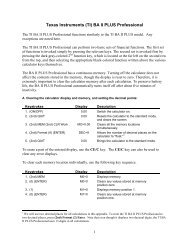
EXAMPLE Tate Company, a fast-growing plastics company, is confronted with six projects
competing for its fixed budget of $250,000. The initial investment and IRR for
each project are as follows:
FIGURE 9.5
Investment
Opportunities Schedule
Investment opportunities
schedule (IOS) for Tate
Company projects
Project Initial investment IRR
A $ 80,000 12%
B 70,000 20
C 100,000 16
D 40,000 8
E 60,000 15
F 110,000 11
The firm has a cost of capital of 10%. Figure 9.5 presents the IOS that results
from ranking the six projects in descending order on the basis of their IRRs.
According to the schedule, only projects B, C, and E should be accepted.
IRR
20%
10%
B
C
E
Budget
Constraint
0 100 200 250 300 400 500
230
Total Investment ($000)
A
F
D
Cost of
Capital
IOS

358 PART 3 Long-Term Investment Decisions
net present value approach
An approach to capital rationing
that is based on the use of
present values to determine the
group of projects that will
maximize owners’ wealth.
Together they will absorb $230,000 of the $250,000 budget. Projects A and F
are acceptable but cannot be chosen because of the budget constraint. Project D
is not worthy of consideration; its IRR is less than the firm’s 10% cost of
capital.
The drawback of this approach is that there is no guarantee that the acceptance
of projects B, C, and E will maximize total dollar returns and therefore
owners’ wealth.
Net Present Value Approach
The net present value approach is based on the use of present values to determine
the group of projects that will maximize owners’ wealth. It is implemented by
ranking projects on the basis of IRRs and then evaluating the present value of the
benefits from each potential project to determine the combination of projects
with the highest overall present value. This is the same as maximizing net present
value, in which the entire budget is viewed as the total initial investment. Any
portion of the firm’s budget that is not used does not increase the firm’s value. At
best, the unused money can be invested in marketable securities or returned to the
owners in the form of cash dividends. In either case, the wealth of the owners is
not likely to be enhanced.
EXAMPLE The group of projects described in the preceding example is ranked in Table 9.7 on
the basis of IRRs. The present value of the cash inflows associated with the projects
is also included in the table. Projects B, C, and E, which together require
$230,000, yield a present value of $336,000. However, if projects B, C, and A
were implemented, the total budget of $250,000 would be used, and the present
value of the cash inflows would be $357,000. This is greater than the return
expected from selecting the projects on the basis of the highest IRRs. Implementing
B, C, and A is preferable, because they maximize the present value for the given
budget. The firm’s objective is to use its budget to generate the highest present
value of inflows. Assuming that any unused portion of the budget does not gain
or lose money, the total NPV for projects B, C, and E would be $106,000
TABLE 9.7 Rankings for Tate Company
Projects
Initial Present value of
Project investment IRR inflows at 10%
B $170,000 20% $112,000
C 100,000 16 145,000
E 60,000 15 79,000
A 80,000 12 100,000
F 110,000 11 126,500
D 40,000 8 36,000
Cutoff point
(IRR10%)

LG5
risk (in capital budgeting)
The chance that a project will
prove unacceptable or, more
formally, the degree of variability
of cash flows.
($336,000$230,000), whereas for projects B, C, and A the total NPV would be
$107,000 ($357,000$250,000). Selection of projects B, C, and A will therefore
maximize NPV.
Review Questions
CHAPTER 9 Capital Budgeting Techniques: Certainty and Risk 359
9–7 What are real options? What are some major types of real options?
9–8 What is the difference between the strategic NPV and the traditional
NPV? Do they always result in the same accept–reject decisions?
9–9 What is capital rationing? In theory, should capital rationing exist? Why
does it frequently occur in practice?
9–10 Compare and contrast the internal rate of return approach and the net
present value approach to capital rationing. Which is better? Why?
Behavioral Approaches for Dealing with Risk
In the context of capital budgeting, the term risk refers to the chance that a project
will prove unacceptable—that is, NPV$0 or IRRcost of capital. More
formally, risk in capital budgeting is the degree of variability of cash flows. Projects
with a small chance of acceptability and a broad range of expected cash
flows are more risky than projects that have a high chance of acceptability and a
narrow range of expected cash flows.
In the conventional capital budgeting projects assumed here, risk stems
almost entirely from cash inflows, because the initial investment is generally
known with relative certainty. These inflows, of course, derive from a number of
variables related to revenues, expenditures, and taxes. Examples include the level
of sales, the cost of raw materials, labor rates, utility costs, and tax rates. We will
concentrate on the risk in the cash inflows, but remember that this risk actually
results from the interaction of these underlying variables.
Behavioral approaches can be used to get a “feel” for the level of project risk,
whereas other approaches explicitly recognize project risk. Here we present a few
behavioral approaches for dealing with risk in capital budgeting: sensitivity and
scenario analysis, decision trees, and simulation. In addition, some international
risk considerations are discussed.
Sensitivity Analysis and Scenario Analysis
Two approaches for dealing with project risk to capture the variability of cash
inflows and NPVs are sensitivity analysis and scenario analysis. As noted in
Chapter 5, sensitivity analysis is a behavioral approach that uses several possible
values for a given variable, such as cash inflows, to assess that variable’s impact
on the firm’s return, measured here by NPV. This technique is often useful in getting
a feel for the variability of return in response to changes in a key variable. In
capital budgeting, one of the most common sensitivity approaches is to estimate

360 PART 3 Long-Term Investment Decisions
scenario analysis
A behavioral approach that
evaluates the impact on the
firm’s return of simultaneous
changes in a number of
variables.
TABLE 9.8 Sensitivity Analysis
of Treadwell’s
Projects A and B
Project A Project B
Initial investment $10,000 $10,000
Annual cash inflows
Outcome
Pessimistic $1,500 $ 0
Most likely 2,000 2,000
Optimistic 2,500 4,000
Range $1,000 $ 4,000
Net present values a
Outcome
Pessimistic $1,409 $10,000
Most likely 5,212 5,212
Optimistic 9,015 20,424
Range $7,606 $30,424
a These values were calculated by using the corresponding
annual cash inflows. A 10% cost of capital and a
15-year life for the annual cash inflows were used.
the NPVs associated with pessimistic (worst), most likely (expected), and optimistic
(best) estimates of cash inflow. The range can be determined by subtracting
the pessimistic-outcome NPV from the optimistic-outcome NPV.
EXAMPLE Treadwell Tire Company, a tire retailer with a 10% cost of capital, is considering
investing in either of two mutually exclusive projects, A and B. Each requires a
$10,000 initial investment, and both are expected to provide equal annual cash
inflows over their 15-year lives. The firm’s financial manager made pessimistic,
most likely, and optimistic estimates of the cash inflows for each project. The
cash inflow estimates and resulting NPVs in each case are summarized in Table
9.8. Comparing the ranges of cash inflows ($1,000 for project A and $4,000 for
B) and, more important, the ranges of NPVs ($7,606 for project A and $30,424
for B) makes it clear that project A is less risky than project B. Given that both
projects have the same most likely NPV of $5,212, the assumed risk-averse decision
maker will take project A because it has less risk and no possibility of loss.
Scenario analysis is a behavioral approach similar to sensitivity analysis but
broader in scope. It evaluates the impact on the firm’s return of simultaneous
changes in a number of variables, such as cash inflows, cash outflows, and the
cost of capital. For example, the firm could evaluate the impact of both high
inflation (scenario 1) and low inflation (scenario 2) on a project’s NPV. Each scenario
will affect the firm’s cash inflows, cash outflows, and cost of capital,
thereby resulting in different levels of NPV. The decision maker can use these

decision trees
A behavioral approach that uses
diagrams to map the various
investment decision alternatives
and payoffs, along with their
probabilities of occurrence.
FIGURE 9.6
Decision Tree for NPV
Decision Tree for Convoy,
Inc.’s choice between
projects I and J
CHAPTER 9 Capital Budgeting Techniques: Certainty and Risk 361
NPV estimates to assess the risk involved with respect to the level of inflation.
The widespread availability of computer and spreadsheets has greatly enhanced
the use of both scenario and sensitivity analysis.
Decision Trees
Decision trees are a behavioral approach that uses diagrams to map the various
investment decision alternatives and payoffs, along with their probabilities of
occurrence. Their name derives from their resemblance to the branches of a tree
(see Figure 9.6). Decision trees rely on estimates of the probabilities associated
with the outcomes (payoffs) of competing courses of action. The payoffs of each
course of action are weighted by the associated probability; the weighted payoffs
are summed; and the expected value of each course of action is then determined.
The alternative that provides the highest expected value is preferred.
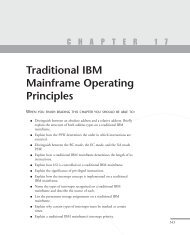
EXAMPLE Convoy, Inc., a manufacturer of picture frames, wishes to choose between two
equally risky projects, I and J. To make this decision, Convoy’s management has
gathered the necessary data, which are depicted in the decision tree in Figure 9.6.
Project I requires an initial investment of $120,000; a resulting expected present
value of cash inflows of $130,000 is shown in column 4. Project I’s expected net
present value, which is calculated below the decision tree, is therefore $10,000.
The expected net present value of project J is determined in a similar fashion.
Project J is preferred because it offers a higher NPV—$15,000.
Decision:
I or J ?
Project I
Project J
Initial
Investment
(1)
$120,000
Expected NPV I $130,000 $120,000 $10,000
Expected NPV J $155,000 $140,000 $15,000
Because Expected NPV J Expected NPV I , Choose J.
Present Value
of Cash Inflow
Probablility (Payoff)
(2)
(3)
.40
.50
.10
$225,000
$100,000
–$100,000
Expected Present Value of Cash Inflows
$140,000
.30
.40
.30
$280,000
$200,000
–$ 30,000
Expected Present Value of Cash Inflows
Weighted
Present Value
of Cash Inflow
[(2) (3)]
(4)
$ 90,000
50,000
–10,000
$130,000
$ 84,000
80,000
–9,000
$155,000

362 PART 3 Long-Term Investment Decisions
simulation
A statistics-based behavioral
approach that applies predetermined
probability distributions
and random numbers to estimate
risky outcomes.
FIGURE 9.7
NPV Simulation
Flowchart of a net present
value simulation
Simulation
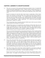
Simulation is a statistics-based behavioral approach that applies predetermined
probability distributions and random numbers to estimate risky outcomes. By
tying the various cash flow components together in a mathematical model and
repeating the process numerous times, the financial manager can develop a probability
distribution of project returns. Figure 9.7 presents a flowchart of the simulation
of the net present value of a project. The process of generating random
numbers and using the probability distributions for cash inflows and cash outflows
enables the financial manager to determine values for each of these variables.
Substituting these values into the mathematical model results in an NPV.
By repeating this process perhaps a thousand times, one can create a probability
distribution of net present values.
Although only gross cash inflows and cash outflows are simulated in Figure
9.7, more sophisticated simulations using individual inflow and outflow components,
such as sales volume, sale price, raw material cost, labor cost, maintenance
expense, and so on, are quite common. From the distribution of returns, the decision
maker can determine not only the expected value of the return but also the
probability of achieving or surpassing a given return. The use of computers has
made the simulation approach feasible. The output of simulation provides an
Probability
Repeat
Generate
Random
Number
Cash Inflows
Mathematical Model
NPV = Present Value of Cash Inflows – Present Value of Cash Outflows
Probability
Probability
Net Present Value (NPV)
Generate
Random
Number
Cash Outflows

exchange rate risk
The danger that an unexpected
change in the exchange rate
between the dollar and the
currency in which a project’s
cash flows are denominated will
reduce the market value of that
project’s cash flow.
transfer prices
Prices that subsidiaries charge
each other for the goods and
services traded between them.
CHAPTER 9 Capital Budgeting Techniques: Certainty and Risk 363
excellent basis for decision making, because it enables the decision maker to view
a continuum of risk–return tradeoffs rather than a single-point estimate.
International Risk Considerations
Although the basic techniques of capital budgeting are the same for multinational
companies (MNCs) as for purely domestic firms, firms that operate in several
countries face risks that are unique to the international arena. Two types of risk
are particularly important: exchange rate risk and political risk.
Exchange rate risk reflects the danger that an unexpected change in the
exchange rate between the dollar and the currency in which a project’s cash flows
are denominated will reduce the market value of that project’s cash flow. The
dollar value of future cash inflows can be dramatically altered if the local currency
depreciates against the dollar. In the short term, specific cash flows can be
hedged by using financial instruments such as currency futures and options.
Long-term exchange rate risk can best be minimized by financing the project, in
whole or in part, in local currency.
Political risk is much harder to protect against. Once a foreign project is
accepted, the foreign government can block the return of profits, seize the firm’s
assets, or otherwise interfere with a project’s operation. The inability to manage
political risk after the fact makes it even more important that managers account
for political risks before making an investment. They can do so either by adjusting
a project’s expected cash inflows to account for the probability of political interference
or by using risk-adjusted discount rates (discussed later in this chapter) in
capital budgeting formulas. In general, it is much better to adjust individual project
cash flows for political risk subjectively than to use a blanket adjustment for
all projects.
In addition to unique risks that MNCs must face, several other special issues
are relevant only for international capital budgeting. One of these special issues is
taxes. Because only after-tax cash flows are relevant for capital budgeting, financial
managers must carefully account for taxes paid to foreign governments on
profits earned within their borders. They must also assess the impact of these tax
payments on the parent company’s U.S. tax liability.
Another special issue in international capital budgeting is transfer pricing.
Much of the international trade involving MNCs is, in reality, simply the shipment
of goods and services from one of a parent company’s subsidiaries to another subsidiary
located abroad. The parent company therefore has great discretion in setting
transfer prices, the prices that subsidiaries charge each other for the goods and
services traded between them. The widespread use of transfer pricing in international
trade makes capital budgeting in MNCs very difficult unless the transfer
prices that are used accurately reflect actual costs and incremental cash flows.
Finally, MNCs often must approach international capital projects from a
strategic point of view, rather than from a strictly financial perspective. For example,
an MNC may feel compelled to invest in a country to ensure continued access,
even if the project itself may not have a positive net present value. This motivation
was important for Japanese automakers who set up assembly plants in the United
States in the early 1980s. For much the same reason, U.S. investment in Europe
surged during the years before the market integration of the European Community

364 PART 3 Long-Term Investment Decisions
FOCUS ON PRACTICE Bestfoods’ Recipe for Risk
With future volume growth in
North America and Western
Europe limited to 3 percent at
most, executives at Bestfoods
(now a unit of the Anglo-Dutch
conglomerate Unilever) decided to
look for more promising markets.
Whereas other food manufacturers
were hesitant to take the international
plunge, Bestfoods took its
popular brands, such as Hellman’s/Best
Foods, Knorr, Mazola,
and Skippy, where the growth
was—emerging markets like Latin
America, where the company
could grow at a rate of 15 percent
a year. At the time it was acquired
by Unilever, Bestfoods derived
about 22 percent of its revenues
outside the United States and
Western Europe, producing mayonnaise,
soups, and other foods for
110 different markets at 130 manufacturing
plants worldwide.
Bestfoods’ international
expansion succeeded because the
company developed methods to
incorporate the risks and rewards
of its foreign investments into proj-
ect analyses. These risks included
exchange rate and political risks,
as well as tax and legal considerations
and strategic issues. First, it
increased its familiarity with the
foreign market by partnering with
other companies whenever possible
and by developing local management
and experience. From
this knowledge base, Bestfoods
was willing to take calculated
risks. Working with consultants,
the company created its own analytical
model to set discount rates
for different markets.
Some companies attempt to
quantify the risk of foreign projects
by arbitrarily assigning a premium
to the discount rate they use for
domestic projects. Executives who
rely on this subjective method may
overestimate the costs of doing
business overseas and rule out
good projects. Unlike these companies,
Bestfoods took the time to
develop specific costs of capital
for international markets. To incorporate
the benefits of diversification
for a multinational company
in 1992. MNCs often invest in production facilities in the home country of major
rivals to deny these competitors an uncontested home market. MNCs also may
feel compelled to invest in certain industries or countries to achieve a broad corporate
objective such as completing a product line or diversifying raw material
sources, even when the project’s cash flows may not be sufficiently profitable.
Review Questions
In Practice
like Bestfoods, the company
adapted the capital asset pricing
model (CAPM). The model factors
in elements of economic and political
risk to obtain the country’s risk
premium and develops betas for
each country on the basis of the
local market’s volatility and its correlation
to the U.S. market. For
example, the high volatility of
Brazil’s market has a low correlation
to the U.S. market, so the
country beta was .81. With the
risk-free rates and country betas,
Bestfoods could calculate local
and global costs of capital. This
more sophisticated approach gave
Bestfoods the confidence to pursue
an aggressive international
strategy that increased shareholder
value and resulted in
Unilever offering a substantial premium
to acquire the company.
Sources: Adapted from Andrew Osterland,
“Lowering the Bar,” CFO (August 1, 2002),
downloaded from www.cfo.com; Stanley
Reed, “Unilever Restocks,” Business Week
International (August 6, 2001), downloaded
from Electric Library, ask.elibrary.com
9–11 Define risk in terms of the cash inflows from a capital budgeting project.
Briefly describe and compare the following behavioral approaches,
explaining how each can be used to deal with project risk: (a) sensitivity
analysis; (b) scenario analysis; (c) decision trees; and (d) simulation.
9–12 Briefly explain how each of the following considerations affects the capital
budgeting decisions of multinational companies: (a) exchange rate risk;
(b) political risk; (c) tax law differences; (d) transfer pricing; and (e) a
strategic rather than strictly financial viewpoint.

LG6
risk-adjusted discount rate
(RADR)
The rate of return that must be
earned on a given project to
compensate the firm’s owners
adequately—that is, to maintain
or improve the firm’s share price.
CHAPTER 9 Capital Budgeting Techniques: Certainty and Risk 365
Risk-Adjusted Discount Rates
The approaches for dealing with risk that have been presented so far enable the
financial manager to get a “feel” for project risk. Unfortunately, they do not
explicitly recognize project risk. We will now illustrate the most popular riskadjustment
technique that employs the net present value (NPV) decision
method. 7 The NPV decision rule of accepting only those projects with NPVs$0
will continue to hold. Close examination of the basic equation for NPV, Equation
9.1, should make it clear that because the initial investment (CF 0) is known
with certainty, a project’s risk is embodied in the present value of its cash inflows:
n
t1
Two opportunities to adjust the present value of cash inflows for risk exist:
(1) The cash inflows (CF t) can be adjusted, or (2) the discount rate (k) can be
adjusted. Adjusting the cash inflows is highly subjective, so here we describe the
more popular process of adjusting the discount rate. In addition, we consider the
practical aspects of risk-adjusted discount rates.
Determining Risk-Adjusted Discount Rates (RADRs)
A popular approach for risk adjustment involves the use of risk-adjusted discount
rates (RADRs). This approach uses Equation 9.1 but employs a risk-adjusted discount
rate, as noted in the following expression:
NPV n
t1
CF t
(1 k) t
CF 0
(9.4)
The risk-adjusted discount rate (RADR) is the rate of return that must be
earned on a given project to compensate the firm’s owners adequately—that is, to
maintain or improve the firm’s share price. The higher the risk of a project, the
higher the RADR, and therefore the lower the net present value for a given stream
of cash inflows. The logic underlying the use of RADRs is closely linked to the capital
asset pricing model (CAPM) developed in Chapter 5. Because the CAPM is
based on an assumed efficient market, which does not exist for real corporate
(nonfinancial) assets such as plant and equipment, the CAPM is not directly
applicable in making capital budgeting decisions. Financial managers therefore
assess the total risk of a project and use it to determine the risk-adjusted discount
rate (RADR), which can be used in Equation 9.4 to find the NPV.
In order not to damage its market value, the firm must use the correct discount
rate to evaluate a project. If a firm discounts a risky project’s cash inflows
at too low a rate and accepts the project, the firm’s market price may drop as
investors recognize that the firm itself has become more risky. On the other hand,
if the firm discounts a project’s cash inflows at too high a rate, it will reject
acceptable projects. Eventually the firm’s market price may drop, because
CF t
(1 RADR) t
7. The IRR could just as well have been used, but because NPV is theoretically preferable, it is used instead.

366 PART 3 Long-Term Investment Decisions
investors who believe that the firm is being overly conservative will sell their
stock, putting downward pressure on the firm’s market value.
Unfortunately, there is no formal mechanism for linking total project risk to
the level of required return. As a result, most firms subjectively determine the
RADR by adjusting their existing required return. They adjust it up or down
depending on whether the proposed project is more or less risky, respectively, than
the average risk of the firm. This CAPM-type of approach provides a “rough estimate”
of the project risk and required return because both the project risk measure
and the linkage between risk and required return are estimates.
EXAMPLE Bennett Company wishes to use the risk-adjusted discount rate approach to
determine, according to NPV, whether to implement project A or project B. In
addition to the data presented earlier, Bennett’s management after much analysis
assigned a “risk index” of 1.6 to project A and of 1.0 to project B. The risk index
is merely a numerical scale used to classify project risk: Higher index values are
assigned to higher-risk projects, and vice versa. The CAPM-type relationship
used by the firm to link risk (measured by the risk index) and the required return
(RADR) is shown in the following table.
Risk index Required return (RADR)
0.0 6% (risk-free rate, RF) 0.2 7
0.4 8
0.6 9
0.8 10
Project B → 1.0 11
1.2 12
1.4 13
Project A → 1.6 14
1.8 16
2.0 18
Because project A is riskier than project B, its RADR of 14% is greater than
project B’s 11%. The net present value of each project, calculated using its
RADR, is found as shown on the time lines in Figure 9.8. The results clearly
show that project B in preferable, because its risk-adjusted NPV of $9,798 is
greater than the $6,063 risk-adjusted NPV for project A. As reflected by the
NPVs in Figure 9.2, if the discount rates were not adjusted for risk, project A
would be preferred to project B.
Calculator Use We can again use the preprogrammed NPV function in a financial
calculator to simplify the NPV calculation. The keystrokes for project A—
the annuity—typically are as shown at the top of the next page. The keystrokes
for project B—the mixed stream—are also shown at the top of the next page.
The calculated NPVs for projects A and B of $6,063 and $9,798, respectively,
agree with those shown in Figure 9.8.

Project A
Input Function
42000 CF 0
14000
5
14
Solution
6063.13
CF 1
N
I
NPV
CHAPTER 9 Capital Budgeting Techniques: Certainty and Risk 367
Project B
Input Function
45000 CF 0
28000
12000
10000
3
11
Solution
9798.43
FIGURE 9.8 Calculation of NPVs for Bennett Company’s Capital Expenditure Alternatives
using RADRs
Time lines depicting the cash flows and NPV calculations using RADRs for projects A and B
Project A
0
$42,000
48,063
NPVA = $ 6,063
$54,798
Project B
0
$45,000
25,225
9,739
7,312
6,587
5,935
NPVB = $ 9,798
1
$14,000
1
$28,000
k = 11%
k = 11%
2
$14,000
2
$12,000
End of Year
k = 14%
End of Year
k = 11%
3
$14,000
3
$10,000
CF 1
CF 2
CF 3
N
I
NPV
k = 11%
4
$14,000
4
$10,000
k = 11%
5
$14,000
5
$10,000
Note: When we use the risk indexes of 1.6 and 1.0 for projects A and B, respectively, along with the table in the middle of the preceding page, a
risk-adjusted discount rate (RADR) of 14% results for project A and a RADR of 11% results for project B.

368 PART 3 Long-Term Investment Decisions
Spreadsheet Use Analysis of projects using risk-adjusted discount rates
(RADRs) also can be calculated as shown on the following Excel spreadsheet.
The usefulness of risk-adjusted discount rates should now be clear. The real
difficulty lies in estimating project risk and linking it to the required return
(RADR).
RADRs in Practice
In spite of the appeal of total risk, RADRs are often used in practice. Their popularity
stems from two facts: (1) They are consistent with the general disposition of
financial decision makers toward rates of return, and (2) they are easily estimated
and applied. The first reason is clearly a matter of personal preference, but the
second is based on the computational convenience and well-developed procedures
involved in the use of RADRs.
In practice, firms often establish a number of risk classes, with an RADR
assigned to each. Each project is then subjectively placed in the appropriate risk
class, and the corresponding RADR is used to evaluate it. This is sometimes done
on a division-by-division basis, in which case each division has its own set of risk
classes and associated RADRs, similar to those for Bennett Company in Table
9.9. The use of divisional costs of capital and associated risk classes enables a
large multidivisional firm to incorporate differing levels of divisional risk into the
capital budgeting process and still recognize differences in the levels of individual
project risk.

CHAPTER 9 Capital Budgeting Techniques: Certainty and Risk 369
TABLE 9.9 Bennett Company’s Risk Classes and RADRs
Risk-adjusted
discount rate,
Risk class Description RADR
I Below-average risk: Projects with low risk. Typically involve
routine replacement without renewal of existing activities.
8%
II Average risk: Projects similar to those currently implemented. 10% a
Typically involve replacement or renewal of existing activities.
III Above-average risk: Projects with higher than normal, but
not excessive, risk. Typically involve expansion of existing or
similar activities.
14%
IV Highest risk: Projects with very high risk. Typically involve
expansion into new or unfamiliar activities.
20%
a This RADR is actually the firm’s cost of capital, which is discussed in detail in Chapter 10. It represents
the firm’s required return on its existing portfolio of projects, which is assumed to be unchanged with
acceptance of the “average risk” project.
EXAMPLE Assume that the management of Bennett Company decided to use risk classes to
analyze projects and so placed each project in one of four risk classes according
to its perceived risk. The classes ranged from I for the lowest-risk projects to IV
for the highest-risk projects. Associated with each class was an RADR appropriate
to the level of risk of projects in the class, as given in Table 9.9. Bennett classified
as lower-risk those projects that tend to involve routine replacement or
renewal activities; higher-risk projects involve expansion, often into new or unfamiliar
activities.
The financial manager of Bennett has assigned project A to class III and project
B to class II. The cash flows for project A would be evaluated using a 14%
RADR, and project B’s would be evaluated using a 10% RADR. 8 The NPV of
project A at 14% was calculated in Figure 9.8 to be $6,063, and the NPV for project
B at a 10% RADR was shown in Figure 9.2 to be $10,924. Clearly, with
RADRs based on the use of risk classes, project B is preferred over project A. As
noted earlier, this result is contrary to the preference shown in Figure 9.2, where
differing risks of projects A and B were not taken into account.
Review Questions
9–13 Describe the logic involved in using risk-adjusted discount rates (RADRs).
How is this approach related to the capital asset pricing model (CAPM)?
Explain.
9–14 How are risk classes often used to apply RADRs?
8. Note that the 10% RADR for project B using the risk classes in Table 9.9 differs from the 11% RADR used in the
preceding example for project B. This difference is attributable to the less precise nature of the use of risk classes.

370 PART 3 Long-Term Investment Decisions
S UMMARY
FOCUS ON VALUE
After estimating the relevant cash flows, the financial manager must apply appropriate
decision techniques to assess whether the project creates value for shareholders. Net
present value (NPV) and internal rate of return (IRR) are the generally preferred capital
budgeting techniques. Both use the cost of capital as the required return needed to compensate
shareholders for undertaking projects with the same risk as that of the firm. Both
indicate whether a proposed investment creates or destroys shareholder value. NPV is the
theoretically preferred approach, but IRR is preferred in practice because of its intuitive
appeal.
Procedures for explicitly recognizing real options embedded in capital projects and
procedures for selecting projects under capital rationing enable the financial manager to
refine the capital budgeting process further. Not all capital budgeting projects have the
same level of risk as the firm’s existing portfolio of projects. The financial manager must
therefore adjust projects for differences in risk when evaluating their acceptability. Riskadjusted
discount rates (RADRs) provide a mechanism for adjusting the discount rate in a
manner consistent with the risk–return preferences of market participants and thereby
accepting only value-creating projects. These techniques should enable the financial manager
to make capital budgeting decisions that are consistent with the firm’s goal of maximizing
stock price.
REVIEW OF LEARNING GOALS
Calculate, interpret, and evaluate the payback
LG1
period. The payback period measures the
exact amount of time required for the firm to
recover its initial investment from cash inflows.
The formula and decision criterion for the payback
period are summarized in Table 9.10. Shorter
payback periods are preferred. In addition to its
ease of calculation and simple intuitive appeal, the
advantages of the payback period lie in its consideration
of cash inflows, the implicit consideration
given to timing, and its ability to measure risk
exposure. Its weaknesses include its lack of linkage
to the wealth maximization goal, failure to explicitly
consider time value, and the fact that it
ignores cash flows that occur after the payback
period.
Apply net present value (NPV) and internal rate
LG2
of return (IRR) to relevant cash flows to choose
acceptable capital expenditures. Sophisticated capital
budgeting techniques use the cost of capital to
consider the time factor in the value of money. Two
such techniques are net present value (NPV) and internal
rate of return (IRR). The key formulas and
decision criteria for these techniques are summarized
in Table 9.10. Both NPV and IRR provide the
same accept–reject decisions but often provide conflicting
ranks.
Use net present value profiles to compare the
LG3
NPV and IRR techniques in light of conflicting
rankings. Net present value profiles are useful in
comparing projects, especially when conflicting

ankings exist between NPV and IRR. On a purely
theoretical basis, NPV is preferred over IRR, because
NPV assumes reinvestment of intermediate
cash inflows at the cost of capital and is not subject
to the mathematical problems that often arise when
one is calculating IRRs for nonconventional cash
flows. In practice, the IRR is more commonly used
because it is consistent with the general preference
toward rates of return.
Discuss two additional considerations in capital
LG4
budgeting—recognizing real options and choosing
projects under capital rationing. By explicitly
recognizing real options—opportunities that are
embedded in capital projects and that allow managers
to alter their cash flow and risk in a way that
effects project acceptability (NPV)—the financial
manager can find a project’s strategic NPV. Some of
the more common types of real options are abandonment,
flexibility, growth, and timing options.
The strategic NPV explicitly recognizes the value of
real options and thereby improves the quality of
the capital budgeting decision.
CHAPTER 9 Capital Budgeting Techniques: Certainty and Risk 371
T ABLE 9.10 Summary of Key Formulas/Definitions and Decision Criteria
for Capital Budgeting Techniques
Technique Formula/definition Decision criteria
Payback period a For annuity:
Initial investment
Annual cash inflow
For mixed stream: Calculate cumulative cash
inflows on year-to-year basis until the initial
investment is recovered.
Net present value (NPV) b Present value of cash inflowsInitial Accept if $0.
investment. Reject if $0.
Internal rate of return (IRR) b The discount rate that causes NPV$0 Accept if the cost of capital.
(present value of cash inflows equals the Reject if the cost of capital.
initial investment).
a Unsophisticated technique, because it does not give explicit consideration to the time value of money.
b Sophisticated technique, because it gives explicit consideration to the time value of money.
Accept if maximum acceptable payback
period.
Reject if maximum acceptable payback
period.
Capital rationing commonly occurs in practice.
Its objective is to select from all acceptable projects
the group that provides the highest overall net present
value but does not require more dollars than are
budgeted. Of the two basic approaches for choosing
projects under capital rationing, the NPV approach
better achieves the objective of using the budget to
generate the highest present value of cash inflows.
Recognize sensitivity analysis and scenario
LG5
analysis, decision trees, and simulation as behavioral
approaches for dealing with project risk,
and the unique risks that multinational companies
face. Risk in capital budgeting is concerned with
either the chance that a project will prove unacceptable
or, more formally, the degree of variability
of cash flows. Sensitivity analysis and scenario
analysis are two behavioral approaches for dealing
with project risk to capture the variability of cash
inflows and NPVs. A decision tree is a behavioral
approach for dealing with risk that relies on estimates
of probabilities associated with the outcomes
of competing courses of action to determine the

372 PART 3 Long-Term Investment Decisions
expected values used to select a preferred action.
Simulation is a statistics-based behavioral approach
that results in a probability distribution of project
returns. It usually requires a computer and allows
the decision maker to understand the risk–return
tradeoffs involved in a proposed investment.
Although the basic capital budgeting techniques
are the same for multinational and purely domestic
companies, firms that operate in several countries
must also deal with both exchange rate and political
risks, tax law differences, transfer pricing, and
strategic rather than strictly financial considerations.
SELF-TEST PROBLEMS (Solutions in Appendix B)
LG1 LG2 LG3
LG6
Understand the calculation and practical as-
LG6
pects of risk-adjusted discount rates (RADRs).
The risk adjusted discount rate (RADR) technique
involves a market-based adjustment of the discount
rate used to calculate NPV. The RADR is closely
linked to the CAPM, but because real corporate assets
are generally not traded in an efficient market,
the CAPM cannot be applied directly to capital
budgeting. RADRs are commonly used in practice
because decision makers prefer rates of return and
find them easy to estimate and apply.
ST 9–1 All techniques with NPV profile—Mutually exclusive projects Fitch Industries
is in the process of choosing the better of two equal-risk, mutually exclusive capital
expenditure projects—M and N. The relevant cash flows for each project are
shown in the following table. The firm’s cost of capital is 14%.
Project M Project N
Initial investment (CF 0) $28,500 $27,000
Year (t) Cash inflows (CF t)
1 $10,000 $11,000
2 10,000 10,000
3 10,000 9,000
4 10,000 8,000
a. Calculate each project’s payback period.
b. Calculate the net present value (NPV) for each project.
c. Calculate the internal rate of return (IRR) for each project.
d. Summarize the preferences dictated by each measure you calculated,
and indicate which project you would recommend. Explain
why.
e. Draw the net present value profiles for these projects on the same set of
axes, and explain the circumstances under which a conflict in rankings
might exist.
ST 9–2 Risk-adjusted discount rates CBA Company is considering two mutually
exclusive projects, A and B. The following table shows the CAPM-type relationship
between a risk index and the required return (RADR) applicable to CBA
Company.

PROBLEMS
LG1
LG1
Project data are shown as follows:
CHAPTER 9 Capital Budgeting Techniques: Certainty and Risk 373
Risk index Required return (RADR)
0.0 7.0% (risk-free rate, RF) 0.2 8.0
0.4 9.0
0.6 10.0
0.8 11.0
1.0 12.0
1.2 13.0
1.4 14.0
1.6 15.0
1.8 16.0
2.0 17.0
Project A Project B
Initial investment (CF0) $15,000 $20,000
Project life 3 years 3 years
Annual cash inflow (CF) $7,000 $10,000
Risk index 0.4 1.8
a. Ignoring any differences in risk and assuming that the firm’s cost of capital is
10%, calculate the net present value (NPV) of each project.
b. Use NPV to evaluate the projects, using risk-adjusted discount rates (RADRs)
to account for risk.
c. Compare, contrast, and explain your findings in parts a and b.
9–1 Payback period Lee Corporation is considering a capital expenditure that
requires an initial investment of $42,000 and returns after-tax cash inflows of
$7,000 per year for 10 years. The firm has a maximum acceptable payback
period of 8 years.
a. Determine the payback period for this project.
b. Should the company accept the project? Why or why not?
9–2 Payback comparisons Dallas Tool has a 5-year maximum acceptable payback
period. The firm is considering the purchase of a new machine and must choose
between two alternative ones. The first machine requires an initial investment of
$14,000 and generates annual after-tax cash inflows of $3,000 for each of the
next 7 years. The second machine requires an initial investment of $21,000 and
provides an annual cash inflow after taxes of $4,000 for 20 years.
a. Determine the payback period for each machine.

374 PART 3 Long-Term Investment Decisions
LG2
LG2
LG2
LG2
b. Comment on the acceptability of the machines, assuming that they are independent
projects.
c. Which machine should the firm accept? Why?
d. Do the machines in this problem illustrate any of the weaknesses of using
payback? Discuss.
9–3 NPV Calculate the net present value (NPV) for the following 20-year projects.
Comment on the acceptability of each. Assume that the firm has an opportunity
cost of 14%.
a. Initial investment is $10,000; cash inflows are $2,000 per year.
b. Initial investment is $25,000; cash inflows are $3,000 per year.
c. Initial investment is $30,000; cash inflows are $5,000 per year.
9–4 NPV for varying costs of capital Cheryl’s Beauty Aids is evaluating a new
fragrance-mixing machine. The machine requires an initial investment of
$24,000 and will generate after-tax cash inflows of $5,000 per year for 8
years. For each of the costs of capital listed, (1) calculate the net present value
(NPV), (2) indicate whether to accept or reject the machine, and (3) explain
your decision.
a. The cost of capital is 10%.
b. The cost of capital is 12%.
c. The cost of capital is 14%.
9–5 Net present value—Independent projects Using a 14% cost of capital, calculate
the net present value for each of the independent projects shown in the following
table, and indicate whether each is acceptable.
Project A Project B Project C Project D Project E
Initial investment (CF 0) $26,000 $500,000 $170,000 $950,000 $80,000
Year (t) Cash inflows (CF t)
1 $4,000 $100,000 $20,000 $230,000 $ 0
2 4,000 120,000 19,000 230,000 0
3 4,000 140,000 18,000 230,000 0
4 4,000 160,000 17,000 230,000 20,000
5 4,000 180,000 16,000 230,000 30,000
6 4,000 200,000 15,000 230,000 0
7 4,000 14,000 230,000 50,000
8 4,000 13,000 230,000 60,000
9 4,000 12,000 70,000
10 4,000 11,000
9–6 NPV and maximum return A firm can purchase a fixed asset for a $13,000 initial
investment. The asset generates an annual after-tax cash inflow of $4,000
for 4 years.
a. Determine the net present value (NPV) of the asset, assuming that the firm
has a 10% cost of capital. Is the project acceptable?

LG2
LG2
CHAPTER 9 Capital Budgeting Techniques: Certainty and Risk 375
b. Determine the maximum required rate of return (closest whole-percentage
rate) that the firm can have and still accept the asset. Discuss this finding in
light of your response in part a.
9–7 NPV—Mutually exclusive projects Jackson Enterprises is considering the
replacement of one of its old drill presses. Three alternative replacement presses
are under consideration. The relevant cash flows associated with each are shown
in the following table. The firm’s cost of capital is 15%.
Press A Press B Press C
Initial investment (CF 0) $85,000 $60,000 $130,000
Year (t) Cash inflows (CF t)
1 $18,000 $12,000 $50,000
2 18,000 14,000 30,000
3 18,000 16,000 20,000
4 18,000 18,000 20,000
5 18,000 20,000 20,000
6 18,000 25,000 30,000
7 18,000 — 40,000
8 18,000 — 50,000
a. Calculate the net present value (NPV) of each press.
b. Using NPV, evaluate the acceptability of each press.
c. Rank the presses from best to worst using NPV.
9–8 Payback and NPV McAllister Products has three projects under consideration.
The cash flows for each of them are shown in the following table. The firm has a
16% cost of capital.
Project A Project B Project C
Initial investment (CF 0) $40,000 $40,000 $40,000
Year (t) Cash inflows (CF t)
1 $13,000 $ 7,000 $19,000
2 13,000 10,000 16,000
3 13,000 13,000 13,000
4 13,000 16,000 10,000
5 13,000 19,000 7,000
a. Calculate each project’s payback period. Which project is preferred according
to this method?
b. Calculate each project’s net present value (NPV). Which project is preferred
according to this method?

376 PART 3 Long-Term Investment Decisions
LG2
LG2
LG2
c. Comment on your findings in parts a and b, and recommend the best project.
Explain your recommendation.
9–9 Internal rate of return For each of the projects shown in the following table, calculate
the internal rate of return (IRR). Then indicate, for each project, the maximum
cost of capital that the firm could have and still find the IRR acceptable.
Project A Project B Project C Project D
Initial investment (CF 0) $90,000 $490,000 $20,000 $240,000
Year (t) Cash inflows (CF t)
1 $20,000 $150,000 $7,500 $120,000
2 25,000 150,000 7,500 100,000
3 30,000 150,000 7,500 80,000
4 35,000 150,000 7,500 60,000
5 40,000 — 7,500 —
9–10 IRR—Mutually exclusive projects Paulus Corporation is attempting to choose
the better of two mutually exclusive projects for expanding the firm’s warehouse
capacity. The relevant cash flows for the projects are shown in the following
table. The firm’s cost of capital is 15%.
Project X Project Y
Initial investment (CF 0) $500,000 $325,000
Year (t) Cash inflows (CF t)
1 $100,000 $140,000
2 120,000 120,000
3 150,000 95,000
4 190,000 70,000
5 250,000 50,000
a. Calculate the IRR to the nearest whole percent for each of the projects.
b. Assess the acceptability of each project on the basis of the IRRs found in part a.
c. Which project, on this basis, is preferred?
9–11 IRR, investment life, and cash inflows Cincinnati Machine Tool (CMT) accepts
projects earning more than the firm’s 15% cost of capital. CMT is currently considering
a 10-year project that provides annual cash inflows of $10,000 and
requires an initial investment of $61,450. (Note: All amounts are after taxes.)
a. Determine the IRR of this project. Is it acceptable?
b. Assuming that the cash inflows continue to be $10,000 per year, how many
additional years would the flows have to continue to make the project acceptable
(that is, to make it have an IRR of 15%)?

LG2
LG1 LG2
LG2 LG3
CHAPTER 9 Capital Budgeting Techniques: Certainty and Risk 377
c. With the given life, initial investment, and cost of capital, what is the minimum
annual cash inflow that the firm should accept?
9–12 NPV and IRR Lilo Manufacturing has prepared the following estimates for a
long-term project it is considering. The initial investment is $18,250, and the
project is expected to yield after-tax cash inflows of $4,000 per year for 7 years.
The firm has a 10% cost of capital.
a. Determine the net present value (NPV) for the project.
b. Determine the internal rate of return (IRR) for the project.
c. Would you recommend that the firm accept or reject the project? Explain
your answer.
9–13 Payback, NPV, and IRR Bruce Reed Enterprises is attempting to evaluate the
feasibility of investing $95,000 in a piece of equipment that has a 5-year life.
The firm has estimated the cash inflows associated with the proposal as shown
in the following table. The firm has a 12% cost of capital.
Year (t) Cash inflows (CF t)
1 $20,000
2 25,000
3 30,000
4 35,000
5 40,000
a. Calculate the payback period for the proposed investment.
b. Calculate the net present value (NPV) for the proposed investment.
c. Calculate the internal rate of return (IRR), rounded to the nearest whole percent,
for the proposed investment.
d. Evaluate the acceptability of the proposed investment using NPV and IRR.
What recommendation would you make relative to implementation of the
project? Why?
9–14 NPV, IRR, and NPV profiles Candor Enterprises is considering two mutually
exclusive projects. The firm, which has a 12% cost of capital, has estimated its
cash flows as shown in the following table.
Project A Project B
Initial investment (CF 0) $130,000 $85,000
Year (t) Cash inflows (CF t)
1 $25,000 $40,000
2 35,000 35,000
3 45,000 30,000
4 50,000 10,000
5 55,000 5,000

378 PART 3 Long-Term Investment Decisions
LG1 LG2 LG3
LG1 LG2 LG3
a. Calculate the NPV of each project, and assess its acceptability.
b. Calculate the IRR for each project, and assess its acceptability.
c. Draw the NPV profiles for both projects on the same set of axes.
d. Evaluate and discuss the rankings of the two projects on the basis of your
findings in parts a, b, and c.
e. Explain your findings in part d in light of the pattern of cash inflows associated
with each project.
9–15 All techniques—mutually exclusive investment decision Easi Chair Company
is attempting to select the best of three mutually exclusive projects. The initial
investment and after-tax cash inflows associated with these projects are shown
in the following table.
Cash flows Project A Project B Project C
Initial investment (CF0) $60,000 $100,000 $110,000
Cash inflows (CFt), t1 to 5 $20,000 $ 31,500 $ 32,500
a. Calculate the payback period for each project.
b. Calculate the net present value (NPV) of each project, assuming that the firm
has a cost of capital equal to 13%.
c. Calculate the internal rate of return (IRR) for each project.
d. Draw the net present value profiles for these projects on the same set of axes,
and discuss any conflict in ranking that may exist between NPV and IRR.
e. Summarize the preferences dictated by each measure, and indicate which
project you would recommend. Explain why.
9–16 All techniques with NPV profile—Mutually exclusive projects Projects A and
B, of equal risk, are alternatives for expanding the Rosa Company’s capacity.
The firm’s cost of capital is 13%. The cash flows for each project are shown in
the following table.
Project A Project B
Initial investment (CF 0) $80,000 $50,000
Year (t) Cash inflows (CF t)
1 $15,000 $15,000
2 20,000 15,000
3 25,000 15,000
4 30,000 15,000
5 35,000 15,000
a. Calculate each project’s payback period.
b. Calculate the net present value (NPV) for each project.
c. Calculate the internal rate of return (IRR) for each project.
d. Draw the net present value profiles for these projects on the same set of axes,
and discuss any conflict in ranking that may exist between NPV and IRR.

LG1 LG2
LG2
CHAPTER 9 Capital Budgeting Techniques: Certainty and Risk 379
e. Summarize the preferences dictated by each measure, and indicate which
project you would recommend. Explain why.
9–17 Integrative—Complete investment decision Hot Springs Press is considering
the purchase of a new printing press. The total installed cost of the press is $2.2
million. This outlay would be partially offset by the sale of an existing press.
The old press has zero book value, cost $1 million 10 years ago, and can be
sold currently for $1.2 million before taxes. As a result of acquisition of the
new press, sales in each of the next 5 years are expected to increase by $1.6 million,
but product costs (excluding depreciation) will represent 50% of sales. The
new press will not affect the firm’s net working capital requirements. The new
press will be depreciated under MACRS using a 5-year recovery period (see
Table 3.2 on page 89). The firm is subject to a 40% tax rate on both ordinary
income and capital gains. Hot Spring Press’s cost of capital is 11%. (Note:
Assume that both the old and the new press will have terminal values of $0 at
the end of year 6.)
a. Determine the initial investment required by the new press.
b. Determine the operating cash inflows attributable to the new press. (Note: Be
sure to consider the depreciation in year 6.)
c. Determine the payback period.
d. Determine the net present value (NPV) and the internal rate of return (IRR)
related to the proposed new press.
e. Make a recommendation to accept or reject the new press, and justify your
answer.
9–18 Integrative—Investment decision Holliday Manufacturing is considering the
replacement of an existing machine. The new machine costs $1.2 million and
requires installation costs of $150,000. The existing machine can be sold currently
for $185,000 before taxes. It is 2 years old, cost $800,000 new, and has a
$384,000 book value and a remaining useful life of 5 years. It was being depreciated
under MACRS using a 5-year recovery period (see Table 3.2 on page 89)
and therefore has the final 4 years of depreciation remaining. If it is held until
the end of 5 years, the machine’s market value will be $0. Over its 5-year life,
the new machine should reduce operating costs by $350,000 per year. The new
machine will be depreciated under MACRS using a 5-year recovery period (see
Table 3.2 on page 89). The new machine can be sold for $200,000 net of
removal and clean up costs at the end of 5 years. An increased investment in net
working capital of $25,000 will be needed to support operations if the new
machine is acquired. Assume that the firm has adequate operating income
against which to deduct any loss experienced on the sale of the existing machine.
The firm has a 9% cost of capital and is subject to a 40% tax rate on both ordinary
income and capital gains.
a. Develop the relevant cash flows needed to analyze the proposed
replacement.
b. Determine the net present value (NPV) of the proposal.
c. Determine the internal rate of return (IRR) of the proposal.
d. Make a recommendation to accept or reject the replacement proposal, and
justify your answer.
e. What is the highest cost of capital that the firm could have and still accept the
proposal? Explain.

380 PART 3 Long-Term Investment Decisions
LG4
LG4
9–19 Real options and the strategic NPV Jenny Rene, the CFO of Asor Products,
Inc., has just completed an evaluation of a proposed capital expenditure for
equipment that would expand the firm’s manufacturing capacity. Using the traditional
NPV methodology, she found the project unacceptable because
NPVtraditional$1,700$0 Before recommending rejection of the proposed project, she has decided to assess
whether there might be real options embedded in the firm’s cash flows. Her evaluation
uncovered the following three options.
Option 1: Abandonment—The project could be abandoned at the end of 3
years, resulting in an addition to NPV of $1,200.
Option 2: Expansion—If the projected outcomes occurred, an opportunity to
expand the firm’s product offerings further would occur at the end of 4 years.
Exercise of this option is estimated to add $3,000 to the project’s NPV.
Option 3: Delay—Certain phases of the proposed project could be delayed if
market and competitive conditions caused the firm’s forecast revenues to
develop more slowly than planned. Such a delay in implementation at that
point has a NPV of $10,000.
Rene estimated that there was a 25% chance that the abandonment option
would need to be exercised, a 30% chance the expansion option would be exercised,
and only a 10% chance that the implementation of certain phases of the
project would have to be delayed.
a. Use the information provided to calculate the strategic NPV, NPVstrategic, for
Asor Products’ proposed equipment expenditure.
b. Judging on the basis of your findings in part a, what action should Rene
recommend to management with regard to the proposed equipment
expenditures?
c. In general, how does this problem demonstrate the importance of considering
real options when making capital budgeting decisions?
9–20 Capital rationing—IRR and NPV approaches Bromley and Sons is attempting
to select the best of a group of independent projects competing for the firm’s fixed
capital budget of $4.5 million. The firm recognizes that any unused portion of this
budget will earn less than its 15% cost of capital, thereby resulting in a present
value of inflows that is less than the initial investment. The firm has summarized
the key data to be used in selecting the best group of projects in the following table.
Present value of
Project Initial investment IRR inflows at 15%
A $5,000,000 17% $5,400,000
B 800,000 18 1,100,000
C 2,000,000 19 2,300,000
D 1,500,000 16 1,600,000
E 800,000 22 900,000
F 2,500,000 23 3,000,000
G 1,200,000 20 1,300,000

LG4
LG5
CHAPTER 9 Capital Budgeting Techniques: Certainty and Risk 381
a. Use the internal rate of return (IRR) approach to select the best group of
projects.
b. Use the net present value (NPV) approach to select the best group of
projects.
c. Compare, contrast, and discuss your findings in parts a and b.
d. Which projects should the firm implement? Why?
9–21 Capital rationing—NPV approach A firm with a 13% cost of capital must
select the optimal group of projects from those shown in the following table,
given its capital budget of $1 million.
NPV at 13%
Project Initial investment cost of capital
A $300,000 $ 84,000
B 200,000 10,000
C 100,000 25,000
D 900,000 90,000
E 500,000 70,000
F 100,000 50,000
G 800,000 160,000
a. Calculate the present value of cash inflows associated with each
project.
b. Select the optimal group of projects, keeping in mind that unused funds are
costly.
9–22 Basic sensitivity analysis Renaissance Pharmaceutical is in the process of evaluating
two mutually exclusive additions to its processing capacity. The firm’s
financial analysts have developed pessimistic, most likely, and optimistic estimates
of the annual cash inflows associated with each project. These estimates
are shown in the following table.
Project A Project B
Initial investment (CF 0) $8,000 $8,000
Outcome Annual cash inflows (CF)
Pessimistic $ 200 $ 900
Most likely 1,000 1,000
Optimistic 1,800 1,100
a. Determine the range of annual cash inflows for each of the two projects.
b. Assume that the firm’ s cost of capital is 10% and that both projects have 20year
lives. Construct a table similar to this for the NPVs for each project.
Include the range of NPVs for each project.
c. Do parts a and b provide consistent views of the two projects? Explain.
d. Which project do you recommend? Why?

382 PART 3 Long-Term Investment Decisions
LG5
LG5
LG5
9–23 Sensitivity analysis James Secretarial Services is considering the purchase of
one of two new personal computers, P and Q. Both are expected to provide benefits
over a 10-year period, and each has a required investment of $3,000. The
firm has a 10% cost of capital. Management has constructed the following table
of estimates of annual cash inflows for pessimistic, most likely, and optimistic
results.
Computer P Computer Q
Initial investment (CF 0) $3,000 $3,000
Outcome Annual cash inflows (CF)
Pessimistic $ 500 $ 400
Most likely 750 750
Optimistic 1,000 1,200
a. Determine the range of annual cash inflows for each of the two computers.
b. Construct a table similar to this for the NPVs associated with each outcome
for both computers.
c. Find the range of NPVs, and subjectively compare the risks associated with
purchasing these computers.
9–24 Decision trees The Ouija Board-Games Company can bring out one of two
new games this season. The Signs Away game has a higher initial cost but also a
higher expected return. Monopolistic Competition, the alternative, has a slightly
lower initial cost but also a lower expected return. The present values and probabilities
associated with each game are listed in the table.
Initial Present value
Game investment of cash inflows Probabilities
Signs Away $140,000 1.00
$320,000 .30
220,000 .50
80,000 .20
Monopolistic Competition $120,000 1.00
$260,000 .20
200,000 .45
50,000 .35
a. Construct a decision tree to analyze the games.
b. Which game do you recommend (following a decision-tree analysis)?
c. Has your analysis captured the differences in the risks associated with these
games? Explain.
9–25 Simulation Wales Castings has compiled the following information on a capital
expenditure proposal:
(1) The projected cash inflows are normally distributed with a mean of $36,000
and a standard deviation of $9,000.

LG6
LG6
CHAPTER 9 Capital Budgeting Techniques: Certainty and Risk 383
(2) The projected cash outflows are normally distributed with a mean of
$30,000 and a standard deviation of $6,000.
(3) The firm has an 11% cost of capital.
(4) The probability distributions of cash inflows and cash outflows are not
expected to change over the project’s 10-year life.
a. Describe how the foregoing data can be used to develop a simulation model
for finding the net present value of the project.
b. Discuss the advantages of using a simulation to evaluate the proposed
project.
9–26 Risk-adjusted discount rates—Basic Country Wallpapers is considering investing
in one of three mutually exclusive projects, E, F, and G. The firm’s cost of
capital, k, is 15%, and the risk-free rate, R F, is 10%. The firm has gathered the
following basic cash flow and risk index data for each project.
Project (j)
E F G
Initial investment (CF 0) $15,000 $11,000 $19,000
Year (t) Cash inflows (CF t )
1 $ 6,000 $ 6,000 $ 4,000
2 6,000 4,000 6,000
3 6,000 5,000 8,000
4 6,000 2,000 12,000
Risk index (RIj) 1.80 1.00 0.60
a. Find the net present value (NPV) of each project using the firm’s cost of capital.
Which project is preferred in this situation?
b. The firm uses the following equation to determine the risk-adjusted discount
rate, RADRj, for each project j:
RADRjR F[RIj(kR F)]
where
RFrisk-free rate of return
RIjrisk index for project j
kcost of capital
Substitute each project’s risk index into this equation to determine its RADR.
c. Use the RADR for each project to determine its risk-adjusted NPV. Which
project is preferable in this situation?
d. Compare and discuss your findings in parts a and c. Which project do you
recommend that the firm accept?
9–27 Risk-adjusted discount rates—Tabular After a careful evaluation of investment
alternatives and opportunities, Joely Company has developed a CAPM-type relationship
linking a risk index to the required return (RADR), as shown in the following
table.

384 PART 3 Long-Term Investment Decisions
LG6
Risk index Required return (RADR)
0.0 7.0% (risk-free rate, RF) 0.2 8.0
0.4 9.0
0.6 10.0
0.8 11.0
1.0 12.0
1.2 13.0
1.4 14.0
1.6 15.0
1.8 16.0
2.0 17.0
The firm is considering two mutually exclusive projects, A and B. The following
are the data the firm has been able to gather about the projects.
Project A Project B
Initial investment (CF0) $20,000 $30,000
Project life 5 years 5 years
Annual cash inflow (CF) $7,000 $10,000
Risk index 0.2 1.4
All the firm’s cash inflows have already been adjusted for taxes.
a. Evaluate the projects using risk-adjusted discount rates.
b. Discuss your findings in part a, and recommend the preferred project.
9–28 Risk classes and RADR Attila Industries is attempting to select the best of
three mutually exclusive projects, X, Y, and Z. Though all the projects have 5year
lives, they possess differing degrees of risk. Project X is in class V, the highest-risk
class; project Y is in class II, the below-average-risk class; and project Z
is in class III, the average-risk class. The basic cash flow data for each project
and the risk classes and risk-adjusted discount rates (RADRs) used by the firm
are shown in the following tables.
Project X Project Y Project Z
Initial investment (CF 0) $180,000 $235,000 $310,000
Year (t) Cash inflows (CF t)
1 $ 80,000 $ 50,000 $ 90,000
2 70,000 60,000 90,000
3 60,000 70,000 90,000
4 60,000 80,000 90,000
5 60,000 90,000 90,000

CHAPTER 9 Capital Budgeting Techniques: Certainty and Risk 385
Risk Classes and RADRs
Risk-adjusted
Risk Class Description discount rate (RADR)
I Lowest risk 10%
II Below-average risk 13
III Average risk 15
IV Above-average risk 19
V Highest risk 22
a. Find the risk-adjusted NPV for each project.
b. Which project, if any, would you recommend that the firm
undertake?
CHAPTER 9 CASE Making Norwich Tool’s Lathe Investment Decision
Norwich Tool, a large machine shop, is considering replacing one of its
lathes with either of two new lathes—lathe A or lathe B. Lathe A is a
highly automated, computer-controlled lathe; lathe B is a less expensive lathe
that uses standard technology. To analyze these alternatives, Mario Jackson, a
financial analyst, prepared estimates of the initial investment and incremental
(relevant) cash inflows associated with each lathe. These are shown in the following
table.
Lathe A Lathe B
Initial investment (CF 0) $660,000 $360,000
Year (t) Cash inflows (CF t)
1 $128,000 $ 88,000
2 182,000 120,000
3 166,000 96,000
4 168,000 86,000
5 450,000 207,000
Note that Mario plans to analyze both lathes over a 5-year period. At the end of
that time, the lathes would be sold, thus accounting for the large fifth-year cash
inflows.
One of Mario’s dilemmas centered on the risk of the two lathes. He believes
that although the two lathes are equally risky, lathe A has a much higher chance
of breakdown and repair because of its sophisticated and not fully proven solidstate
electronic technology. Mario is unable to quantify this possibility effectively,
so he decides to apply the firm’s 13% cost of capital when analyzing the
lathes. Norwich Tool requires all projects to have a maximum payback period of
4.0 years.

386 PART 3 Long-Term Investment Decisions
Required
a. Use the payback period to assess the acceptability and relative ranking of
each lathe.
b. Assuming equal risk, use the following sophisticated capital budgeting techniques
to assess the acceptability and relative ranking of each lathe:
(1) Net present value (NPV).
(2) Internal rate of return (IRR).
c. Summarize the preferences indicated by the techniques used in parts a and b,
and indicate which lathe you recommend, if either, (1) if the firm has unlimited
funds and (2) if the firm has capital rationing.
d. Repeat part b assuming that Mario decides that because of its greater risk,
lathe A’s cash inflows should be evaluated by using a 15% cost of capital.
e. What effect, if any, does recognition of lathe A’s greater risk in part d have
on our recommendation in part c?
WEB EXERCISE Go to the Web site www.arachnoid.com/lutusp/finance_old.html. Page down to
the portion of this screen that contains the financial calculator.
WWW
1. To determine the internal rate of return (IRR) of a project whose initial
investment was $5,000 and whose cash inflows are $1,000 per year for the
next 10 years, perform the steps outlined below. By entering various interest
rates, you will eventually get a present value of $5,000. When this happens
you, have determined the IRR of the project.
To get started, into PV, enter 0; into FV, enter 0; into np, enter 1000;
into pmt, enter 10; and then into ir, enter 8. Click on Calculate PV. This
gives you a number much greater than $5,000. Now change ir to 20 and
then click on Calculate PV. Keeping changing the ir until PV $5,000, the
same as the initial investment.
2. Try another project. The initial investment is $10,000. The cash inflows are
$2,500 per year for the next 6 years. What is its IRR?
3. To calculate the IRR of an investment of $3,000 with a single cash inflow of
$4,800 to be received exactly 3 years after the investment, do the following:
Into FV, enter 4800; into np, enter 3; into pmt, enter 0; and then into ir,
enter 8. Then click on Calculate PV. As before, keep changing ir until the PV
is equal to the initial investment of $3,000. What is this investment’s IRR?
Remember to check the book’s Web site at
www.aw.com/gitman
for additional resources, including additional Web exercises.