LANDSLIDE ASSESSMENT OF THE STARCˇA BASIN (CROATIA ...

LANDSLIDE ASSESSMENT OF THE STARČA BASIN 

(CROATIA) USING MACHINE LEARNING ALGORITHMS 

MILOS ˘ MARJANOVIC, ´ MILOS ˘ KOVACEVIC, ˘ ´ BRANISLAV BAJAT, 

SNJEZANA ˘ 

MIHALIC ´ and BILJANA ABOLMASOV 

about the authors 

Miloš Marjanović 

Palacky University, 

Faculty of Science 

Tř. Svobodý 26, 77 146 Olomouc, Czech Republic 

E-mail: milos.marjanovic01@upol.cz 

Miloš Kovačević 

University of Belgrade, 

Faculty of Civil Engineering 

Bulevar kralja Aleksandra 73, 11000 Belgrade, Serbia 

E-mail: milos@grf.bg.ac.rs 

Branislav Bajat 


Faculty of Civil Engineering 

Bulevar kralja Aleksandra 73, 11000 Belgrade, Serbia 

E-mail: bajat@grf.bg.ac.rs 

Snježana Mihalić 

University of Zagreb, 

Faculty of Mining, Geology and Petroleum Engineering 

Pierottijeva 6, p.p. 390, 10000 Zagreb, Croatia 

E-mail: smihalic@rgn.hr 

corresponding author 

Biljana Abolmasov 


Faculty of Mining and Geology 

Đušina 7, 11000 Belgrade, Serbia 

E-mail: biljana@rgf.bg.ac.rs 

Abstract 

In this research, machine learning algorithms were 

compared in a landslide-susceptibility assessment. Given 

the input set of GIS layers for the Starča Basin, which 

included geological, hydrogeological, morphometric, and 

environmental data, a classification task was performed 

to classify the grid cells to: (i) landslide and non-landslide 

cases, (ii) different landslide types (dormant and abandoned, 

stabilized and suspended, reactivated). After 

finding the optimal parameters, C4.5 decision trees and 

Support Vector Machines were compared using kappa 

statistics. The obtained results showed that classifiers 

were able to distinguish between the different landslide 

types better than between the landslide and non-landslide 

instances. In addition, the Support Vector Machines classifier 

performed slightly better than the C4.5 in all the 

experiments. Promising results were achieved when classifying 

the grid cells into different landslide types using 20% 

of all the available landslide data for the model creation, 

reaching kappa values of about 0.65 for both algorithms. 

Keywords 

landslides, support vector machines, decision trees classifier, 

Starča Basin 

1 INTRODUCTION 

Prior to any conceptualizing and modeling, dealing 

with the landslide phenomenology requires a profound 

understanding of the triggering and conditioning factors 

that are in control of the landslide process. Difficulties 

in landslide-assessment practice arise from the temporal 

and spatial variability of the triggering and conditioning 

factors and the changes in the nature of their interaction 

[1]. This research concentrates only on the spatial aspect 

of landslide distribution, i.e., delimiting landslide-prone 

areas, also known as landslide-susceptibility zoning. 

Only selected conditioning factors (geological, hydrological, 

morphological, anthropogenic, etc.) addressing 

natural ground properties and environmental conditions 

were included in the investigation. 

A conceptual standard developed for the landslide assessment 

[2] was adhered to, and this involved: (i) generation 

of a landslide inventory, (ii) identification and modeling 

of a set of natural factors that are indirectly conditioning 

the slope instability, (iii) estimation of the relative 

contribution of these factors in generating slope failures, 

and (iv) classification of land surface into domains of 

different susceptibility degrees, in our case with respect 

ACTA GEOTECHNICA SLOVENICA, 2011/2 45.

M. MARJANOVIĆ ET AL.: LANDSLIDE ASSESSMENT OF THE STAR˘CA BASIN (CROATIA) USING MACHINE LEARNING ALGORITHMS 

to (i). The essential idea behind it suggests that if there 

were landslide occurrences under certain conditions 

in the past, it is quite likely that a similar association of 

conditions will lead to new occurrences [2]. The estimation 

of the relative contribution of a factor in the overall 

stability (iii) (which herein comes down to a classification 

problem) ranges over a broad variety of methods [3]. 

These include the Analytical Hierarchy Process (AHP) 

[4], conditional probability [5], discriminant analysis [6], 

different kinds of regression models [7], Fuzzy Logics [8], 

Support Vector Machines (SVMs) [9], Artificial Neural 

Networks (ANNs) [10] and decision trees [11]. Relatively 

few researchers have dealt with the machine learning 

approach, but recently it is getting more popular in geoscientific 

communities, especially for comparative studies 

of landslide susceptibility [12], [13]. 

Following such a trend, we herein utilized C4.5 decision 

trees and SVM algorithms for mapping landslides and 

distinguishing between different landslide categories. 

Thus far, researchers did not experiment with multiclass 

classifications (usually binary classification case 

studies can be found in the literature) and here we challenged 

the classification in that context. The theoretical 

advantages of the chosen machine learning approaches 

are numerous, particularly regarding the handling of 

data with different scales and types, independence from 

statistical distribution assumptions (the drawbacks of 

regression and discriminant methods) and so forth [14], 

which was also one of the motifs for its implementation 

in present research. 

The proposed model might serve for a landslidesusceptibility 

assessment in other areas of the City of 

Zagreb, under the assumption of similar terrain properties, 

primarily geological ones. These are urbanized and 

densely populated areas, hence less explorative for the 

field investigation of landslides. In such circumstances, 

the presented approach might lead to certain benefits, 

but more detailed investigations are needed to obtain 

reliable results. The latter involves testing the model 

against several pilot areas and tracking its performance. 

The biggest obstacle to the completion of that goal is a 

lack of detailed landslide inventories at the moment. 

2 METHODS 

The different stages of research called for different 

procedures, imposing a variety of methods, including 

the pre-processing of input attributes, machine learning 

implementation, and performance evaluation. All the 

related machine learning experiments and the subsequent 

algorithm-performance evaluation were placed in 

an open-source package, Weka 3.6 [15]. 

46. ACTA GEOTECHNICA SLOVENICA, 2011/2 

Assuming that our inputs are organized as raster sets 

where each grid element (pixel) represents a data instance 

at a certain point of the terrain, our approach leads to a 

classification task that places each pixel from any terrain 

attribute raster into an appropriate landslide category 

associated with that particular pixel. We will herein 

explain the classification problem and machine learning 

solution in depth, and from the perspective of their particular 

application in landslide-susceptibility assessment. 

2.1 PROBLEM FORMULATION 

Let P={x|xÎR n } be a set of all the possible pixels extracted 

from the raster representation of a given terrain. Each 

pixel is represented as an n-dimensional real vector 

where the coordinate x i represents a value of the i-th 

terrain attribute associated with the pixel x. Further, let 

C={c 1,c 2,…,c l} be a set of l disjunctive, predefined landslide 

categories (j=1,l). A function ¦ c:P→C is called a classification 

if for each x iÎP it holds that ¦ c(x i)=j whenever 

a pixel x i belongs to the landslide category c j. In practice, 

for a given terrain, one has a limited set of m-labeled 

examples (i=1,m) which form a training set (x i, c i), x iÎR n , 

c iÎC, i=1,…,m (m being a reasonably small number of 

instances). The machine learning approach tries to find a 

decision function ¦ c’ which is a good approximation of a 

real, unknown function ¦ c , using only the examples from 

the training set and a specific learning method [16]. 

2.2 SUPPORT VECTOR MACHINES CLAS- 

SIFIER 

Originally, a SVM is a linear binary classifier (instances 

could be classified to only one of the two classes), but 

one can easily transform an n-classes problem into a 

sequence of n (one-versus-all) or n(n-1)/2 (one-versusone) 

binary classification tasks, where using different 

voting schemes leads to a final decision [17]. Given a 

binary training set (x i ,y i), x iÎR n , y iÎ {-1,1}, i=1,…,m, the 

basic variant of the SVM algorithm attempts to generate 

a separating hyper-plane in the original space of n coordinates 

(x i parameters in vector x) between two distinct 

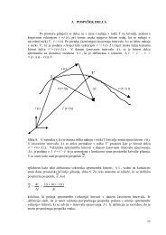
classes (Fig. 1). During the training phase the algorithm 

seeks out a hyper-plane that best separates the samples of 

binary classes (classes 1 and –1). Let h 1: wx + b = 1 and 

h -1: wx + b = –1 (w,xÎR n , bÎR) be possible hyper-planes 

such that the majority of class 1 instances lie above h 1 

(wx + b > 1) and the majority of class –1 fall below h -1 

(wx + b < –1), whereas the elements belonging to h 1, h -1 

are defined as Support Vectors (Fig. 1). Finding another 

hyper-plane h: wx + b = 0 as the best separating (lying in 

the middle of h 1, h -1), assumes calculating w and b, i.e., 

solving the nonlinear convex programming problem.

The notion of the best separation can be formulated as 

finding the maximum margin M between the two classes. 

Since M = 2w -1 maximizing the margin leads to the 

constrained optimization problem of Eq. (1). 

1 

min 

w, 

b 2 


w 

2 

+ Cåe i 

i 

(1) 

w.r.t: 1 -e -y ( w⋅ x + b) £ 0, - e £ 0, i= 1,2,... m 

i i i i 

Despite having some of the instances misclassified (Fig. 

1) it is still possible to balance between the incorrectly 

classified instances and the width of the separating 

margin. In this context, the positive slack variables ε i and 

the penalty parameter C are introduced. Slacks represent 

the distances of the misclassified points to the initial 

hyper-plane, while parameter C models the penalty for 

misclassified training points, that trades-off the margin 

size for the number of erroneous classifications (the 

bigger the C the smaller the number of misclassifications 

and the smaller the margin). The goal is to find a 

hyper-plane that minimizes the misclassification errors 

while maximizing the margin between classes. This 

optimization problem is usually solved in its dual form 

(dual space of Lagrange multipliers): 

* m 

= a y , C 0, i 1,... m 

i 1 

i i i 

³ a 

i 

³ = 

å w x , (2) 

= 

where w* is a linear combination of training examples 

for an optimal hyper-plane. 

However, it can be shown that w* represents a linear 

combination of Support Vectors x i for which the 

corresponding α i Langrangian multipliers are non-zero 

values. Support Vectors for which the C > α i > 0 condi- 

Figure 1. General binary classification case (h 0: wx+b=0; 

h 1: wx+b=1; h 2: wx+b=-1). Shaded points represent misclassified 

instances. 

tion holds, belong either to h 1 or h -1. Let x a and x b be 

two such Support Vectors (C > α a, α b > 0) for which 

y a = 1 and y b = –1. Now b could be calculated from 

b* = –0.5w*(x a + x b), so that the classification (decision) 

function finally becomes: 

x = 

m 

åai 

i= 

1 

i xi⋅ x + 

* 

. (3) 

f( ) sgn y ( ) b 

In order to cope with non-linearity even further, one 

can propose the mapping of instances to a so-called 

feature space of very high dimension: ϕ:R n →R d , n


the dataset. The interpretability of the derived model 

enables a domain expert to have a better understanding 

of the problem and in many cases could be preferable to 

functional models such as SVMs. 

Let us briefly explain how the tree can be derived from 

the training data (x i ,c i), i=1,…,m, where c i is one of k 

disjunctive classes. C4.5 deals both with numerical and 

categorical attributes, but for the sake of simplicity we first 

made an assumption that all attributes are categorical. 

The tree construction process performs a greedy search in 

the space of all possible trees starting from the empty tree 

and adding new nodes in order to increase the classification 

accuracy on the training set. A new node (candidate 

attribute test) is added below a particular branch if the 

instances following the branch are partitioned after the 

test in such way that the distinction between the classes 

becomes more evident. If the test on attribute A splits the 

instances into subsets in which all elements have the same 

class labels that would be a perfect attribute choice (those 

subsets become leaf nodes). On the other hand, if the 

instances are distributed so that in each subset there are 

equal numbers of elements belonging to different classes, 

then A would be the worst attribute choice. Hence, the 

root node should be tested against the most informative 

attribute concerning the whole training set. C4.5 uses the 

Gain Ratio measure [21] to choose between the available 

attributes and is heavily dependent on the notion of 

Entropy. Fig. 2 explains the calculation of Gain Ratio. 

Let Sin be the set of N instances for which the preceding 

test in the parent node forwarded them to the current 

node. Further, let ni be the number of instances from 

Sin that belong to class ci, i=1,...,k. The entropy E(Sin) is 

defined as a measure of impurity (with respect to the 

class label) of the set Sin as: 

k ni ni 

ES ( in ) =-å log2 

(6) 

N N 

i= 

1 

Figure 2. Calculating Gain Ratio of an attribute in the internal 

node of the growing tree. 


If all instances belong to the same class then the entropy 

is zero. On the other hand, if all classes are equally 

present, the entropy is a maximum (log 2k). In our 

problem the setting A denotes the candidate attribute 

of an instance x. Since by assumption A is categorical 

and can take n different values ν 1,ν 2,…,ν n , there are n 

branches leading from the current node. Each S out(A=ν i) 

represents the set of instances for which A takes the 

value ν i . The informative capacity of A concerning the 

classification into k predefined classes can be expressed 

by using the notion of Information Gain: 

S ( A= v) 

IG(S , A) = E(S ) - å E(S ( A = v)) 

(7) 

out 

in in 

vÎ{ v1,..., vn} 

N 

out 

In Eq. (7) |S out(A=ν)| represents the number of instances 

in the set S out(A=ν) and E(S out(A=ν)) is the entropy of 

that set calculated using Eq. (6). The higher is the IG, 

the more informative is the A for the classification in the 

current node, and vice versa [14]. 

The main disadvantage of the IG measure is that it favors 

attributes with many values over those with fewer. This 

leads to wide trees with many branches starting from 

corresponding nodes. If the tree is complex and has a 

lot of leaf nodes, then it is expected that the model will 

overfit the data (it will learn the anomalies of the training 

data and its generalization capacity, i.e., the classification 

accuracy on unseen instances, will be decreased). 

In order to reduce the effect of overfitting C4.5 further 

normalizes IG by the entropy calculated with respect to 

the attribute values instead of class labels (Split Information) 

to obtain the Gain Ratio (GR): 

S out ( A= v) S out ( A= v) 

SI(S in , A) 

=- å log 2 

vÎ{ v1,... vn} 

N N 

, 

IG(S in , A) 

GR(S in , A) 

= 

SI(S , A) 

(8) 

C4.5 uses GR to drive the greedy search over all possible 

trees. If the attribute is numerical (this is the case for 

most attributes in our application) C4.5 detects the 

candidate thresholds that separate the instances into 

different classes. Let (A, c i) pairs be (50, 0), (60, 1), (70,1) 

(80,1), (90,0) ,(100,0). C4.5 identifies two thresholds on 

the boundaries of different classes: A


well as possible (overfitted model) it converts the tree into 

a set of equivalent rules, one rule of the form if A=v and 

B


border of the City of Zagreb, Croatia (Fig. 3). This area 

is composed of the Upper Miocene and Plio-Quaternary 

sediments. The ground conditions, morphological 

settings and urbanization of the area could be considered 

as the primary causal factors for numerous shallow 

and relatively small landslides triggered by physical (e.g., 

intense, short period rainfall) or man-made processes. 

The resources for generating the input dataset of the 

Starča Basin included: landslide inventory; Digital Terrain 

Model (DTM); geological map; hydrogeological map; and 

a land-cover map. From the above-mentioned resources, 

the input dataset was generated as an assembly of attributes. 

Using the advantages of GIS software platforms 

(ArcGIS and SagaGIS) the input data were processed, 

i.e., referenced and normalized (where applicable) and 

stored in a raster image format so that every pixel (every 

center node of the pixel to be more exact) represents 

one instance. Every attribute within the input dataset 

contained 122513 instances with a 10-m cell resolution. 

3.1 LANDSLIDE INVENTORY 

A detailed geomorphological landslide map was 

prepared through a systematic field survey (in the period 

of March–April 2004) at 1:5000 scale (Fig. 4). The total 

mapped landslide area reached only 0.87 km 2 (or 7.1% of 

the study area, which is statistically speaking, an undesirable 

proportion), with a density of about 0.1 slope 

failures per km 2 . The landslide inventory was prepared 

in the form of a GIS database in which information on 

the location, features and abundance of 230 mapped 

landslides is archived [26]. The main landslide characteristics 

were described according to standard WP/WLI 

(1993) recommendations [27]. Landslides were classified 

as (shallow) slide type according to Cruden and Varnes 

Classification [28], with the age and state of activity 

determined according to the morphological indicators. 

Active, suspended and reactivated landslides have clearly 

recognizable fresh scars, without any vegetation cover, 

because of movement within the past few years (59 

slides). Most of the landslides are inactive and they are 

classified as: dormant landslides (95 slides) have recognizable 

scars covered by vegetation during the period of 

inactivity; abandoned landslides (72 slides) are characterised 

by a hummocky surface topography and relics of 

scars completely smoothed during the period of inactivity; 

and stabilized landslides included those mitigated 

by engineering measures (4 slides). Relict landslides (40 

slides) are difficult to recognize, because the only indicator 

of movement is a typical roughly undulating slope 

morphology: concave depletion zone in the upper part 

and convex accumulation zone in the lower part. 


a) 

b) 

Figure 4. a) Landslide distribution in the basin area, b) 

Enlargement of a geomorphological landslide map, original 

scale 1:5000. 

The size of the landslides varies from 270 m 2 to 25.073 

m 2 . Most of the landslides range in size from 400 m 2 to 

1600 m 2 . Regarding activity style, there are single movements 

(150 slides) as well as complex, composite, successive 

and multiple movements (120 slides). ‘Parent-child’ 

relationships were also defined during the mapping. 

The relict slides are excluded from any further analysis 

because of the mapping uncertainty. 

For the purpose of this research, the landslide inventory 

is used only in a raster-image form. The landslide 

inventory was somewhat simplified for the purpose of 

this research in order to enhance the statistical representativeness 

of the categories (the merging of the original 

categories was based on the activity stage).

3.2 CONDITIONING FACTORS – TERRAIN 

ATTRIBUTES 

The landslide-conditioning factors involved a variety 

of input layers, some being directly digitized from the 

original thematic maps, others derived from additional 

spatial calculations and modeling. In effect, 15 inputraster 

layers, with the same 10 m cell resolution, were 

available for further analysis. These could be divided 

into three thematic groups: geological, morphological, 

and environmental factors. Note also that the factors 

that turned more dominant in this research are somewhat 

detailed in the description. 

Geological factors included layers derived from the 1:5000 

geological map, indicating the main geological units in the 

area and the approximately located faults [29]: 

a) 


b) c) 

– Lithology (representing 10 rock units as categorical 

classes 1 ) Eight main lithological types can be distinguished 

(Fig. 5a): eluvial clay and silty clay with 

gravel (Quatenary), alluvial gravel with silty clay 

(Quaternary), gravel with silty clay (Plio-Pleistocene), 

coarse-grained sand (Plio-Pleistocene), sandy 

silt and silt (Pontian), marl with silt and calcareous 

siltstone (Pannonian), laminated marl with calcareous 

sandstone (Sarmatian) and marl (Badenian). 

Considering the relatively high proportion of clayey 

and marly units, the lithological model suggests that 

shallow to deep-seated landslides could be hosted on 

a significant part of the area (Fig. 5a) 

– Proximity to the fault lines 

A high precision terrain surface model (±1 m) was 

developed through the photogrammetric technique, in 

Figure 5. a) Attribute lithological units with the breakdown of the percentage proportion of unit groups, 

b) Attribute channel network base levels, c) Attribute altitude above channel network; 

Note that the selection of these three thematic layers corresponds with the three most important attributes in Table 2. 

1 The categorical attributes were extended into n binary attributes, coding n different initial values (e.g., class 1 and 4 of Lithology are coded as 

1000000000 and 0001000000, respectively, while the same classes for Land Use were 1000 and 0001), in order to give equal preference to every class. 



the framework of orthophotomaps production of the 

Zagreb City area, at a scale of 1:5000. The terrain model 

was subsequently transformed to a DTM by means of 

vector-to-raster conversion. A host of morphometric 

parameters with a proven relevance for landslide assessment 

[30] were derived from the DTM: 

– Slope 

– Downslope gradient (ratio of the slope angle and the 

elevation) 

– Aspect 

– Profile Curvature (terrain curvature in the steepest 

slope direction) 

– Plan Curvature (terrain curvature along the contour) 

– Convergence Index (slope angle convergence) 

– LS factor (ratio of the slope length and the length 

standardized by the Universal Soil Loss Equation) 

– Channel network base level elevations are values 

calculated as a vertical difference between the real 

DTM elevations and the elevations of the (interpolated) 

channel network (Fig. 5b). It provides information 

on how far each cell is from the local flow, just 

by interpreting the higher differences as more remote 

than the lower ones (in channel cells the attribute’s 

value is zero, while in non-channel cells the value is 

increasing with the distance from the flow) 

– Altitude above the channel network is another standard 

morphometric terrain attribute, yet sometimes 

important to determine the relief energy based on 

potential energy differences (height differences) 

between each cell and its local erosional basis (Fig. 

5c). It is basically a DTM downshifted by the value of 

the channel cells elevations. 

– Stream Power Index (potential power of the flows 

given by a relation of the local drainage area and the 

local slope gradient) 

– Topographic Wetness Index (topographic water 

retention potential given by a relation of the upslope 

drainage area and the slope gradient) 

Piezometric map, an interpolation of the maximum 

piezometric pressure heads, measured in a rainy period 

of 2004, was used to generate the attribute: 

– Groundwater table depth (depths from the measurements 

of the minimal water levels in wells, interpolated 

by the nearest-neighbor method, ranged by 4 

classes with 0.5 m intervals, i.e., 0–0.5, 0.5–1, 1–1.5 

and >1.5 m) 

The Land Use map was prepared by a direct visual 

interpretation of a 1:5000 orthophoto according to the 

CORINE classification. The map was generalized as the 

attribute: 


– Land Use (a categorical attribute with 4 thematic 

classes, similarly arranged as in the case of Lithology. 

The classes included: Agricultural areas 30%, Artificial 

surfaces 4%, Forests and semi-natural areas 65%, 

Water bodies 1%) 

4 RESULTS AND DISCUSSION 

The experimental design was governed by the characteristics 

of the dataset, particularly the unbalanced distribution 

of the landslide inventory classes. Since the non-landslide 

class turned out to be predominant over all the landslide 

classes combined, the sampling strategy was tuned accordingly. 

Two different dataset cases were induced: 

– S01 with a binary class labels, i.e., class c 1 – absence of 

landslides, and class c 2 – presence of landslides (Fig. 

6a). It contained 20% of the original dataset (randomly 

selected), or 24500 out of 122513 instances. 

– S123 included only landslide instances (Fig. 6b) from 

the original dataset distributed in three different 

classes: c 1 – dormant and abandoned, c 2 – stabilized 

and suspended, and c 3 – reactivated landslides (a 

total of 10500 instances). 

Thus, the classifier trained by the first set was used to 

locate the landslides throughout the area, while the 

classifier trained by the second set was used to discern 

between three landslide types. In this way, featured 

expert judgment is simulated and could be applied to the 

remaining part of the terrain, as well as to the adjacent 

ground. Both sets passed through the identical experimenting 

protocol discussed subsequently. 

For the C4.5 algorithm we used the default parameters 

of Weka explorer: 0.25 for confidence level for pruning, 

while the minimum number of objects in leaf was held 

at 2. The optimization of SVM also comes down to the 

fitting of only two parameters: the margin penalty C and 

the kernel width γ. The parameters are found in a wellestablished 

cross-validation procedure 2 over the training 

set in each performed experiment [31], [32]. It turns out 

that the optimal parameters (C=100, γ=4) are the same 

for all the performed experiments. 

– Experiment#1: testing was performed on S01 (24500 

instances) and S123 (10500 instances) data in a 

single run (no iterations), through 10-fold cross-validation 

(10-CV). The value of the representative κ was 

2 In k-fold cross-validation (k-CV), the entire set is partitioned 

into k disjoint splits of the same size. Validation is completed in k 

iterations, each time using a different split for the validation, and 

merging the remaining k-1 splits for training.

a) 


Figure 6. a) Landslide inventory map for S01, b) Different landslide categories 

(dormant and abandoned 1, stabilized and suspended 2, reactivated 3) for S123. 

obtained directly after the cross-validation was run. 

For the C4.5 algorithm it reached 0.52 in the S01 

and 0.82 in the S123 data set. The SVM algorithm 

reached a very similar performance, i.e., a fraction 

higher in S01 (Table 1), meaning that it is somewhat 

more reliable in mapping landslides but equal in 

discerning between different types of landslides. 

– Experiment#2: Both sets were randomly divided 

into 20–80% splits. The training was performed on 

20% of the data (5000 instances in S01 and 2000 

instances in S123). In order to obtain statistically 

relevant results, five different 20–80% splits were 

generated and the median among the obtained κ 

values was considered as being representative (Table 

1). As expected, the performance drops significantly, 

especially in S01. It is also apparent that SVM is 

slightly better than the C4.5 in this set, while in S123 

the algorithms are leveled. 

– Experiment#3: generating seven 15–85% splits (3800 

instances in S01 and 1500 instances in S123 for training 

purposes), otherwise analogue to the previous. A 

further decrease of the average κ is noticeable, as well 

as a slightly advantageous performance of the SVM 

algorithm (Table 1). 

– Experiment#4: generating ten 10–90% splits (2500 

instances in S01 and 1000 instances in S123), 

otherwise analogous to the previous. The dropping 

trend continues, as κ values became rather temperate 

for both algorithms within both sets (Table 1). 

Viewing the experiment results altogether, a slight 

preference for the SVM over the C4.5 is obvious in both 

S01 and S123 data sets, due to the smaller κ decrements 

(0.03–0.05) with a reduction of the training sample size. 

b) 

Table 1. Performance evaluation of the C4.5 and SVM classifiers 

by κ-index. 

Experiment S01 S123 

C4.5 SVM C4.5 SVM 

#1 (10–CV) 0.52 0.58 0.82 0.82 

#2 (5x20–80%) 0.38 0,47 0.63 0.65 

#3 (7x15–85%) 0.33 0.44 0.58 0.60 

#4 (10x10–90%) 0.31 0.40 0.48 0.55 

In all the experiments the algorithms exhibit a better 

generalization with the S123 set, meaning that they are 

better in categorizing landslides than actually mapping 

them, concerning the present study area and the chosen 

sampling strategy. Preliminary results suggest that using 

the same input attributes, it would be interesting to 

impose the algorithms over adjacent areas (which are 

urbanized, but have similar terrain features) in order to 

suggest to the expert which types of landslides are present 

prior to the real field mapping. 

Since we have been using a classifier based on information 

gain values (C4.5), we evaluated the ranking of the 

input features according to their IG values (Table 2). It 

appears that the most informative layers are Lithology, 

Channel Network Base Elevations, Altitude Above Channel 

Network, while surprisingly Slope turned out to be 

mediocre to low, hand in hand with the terrain Convergence 

Index and Land Use for instance. One possible 

way to explain this is an exaggeration of the geological 

and, to some extent, the hydrogeological influence on the 

landslide occurrence, so that they obscure the effects of 

slope steepness and land use for instance. 



Table 2. Information Gain (IG) ranking of the input layer 

attributes. 

Terrain attribute IG rank 

Lithology 0.06157 1 

Channel Network Base Elevations 0.04034 2 

Groundwater Table 0.0268 7 

Stream Power Index 0.03038 4 

Aspect 0.02828 5 

Altitude above channels 0.03078 3 

Topographic Wetness Index 0.02789 6 

Land Use 0.02129 10 

Downslope Gradient 0.02413 8 

LS factor 0.02241 9 

Slope 0.021 11 

Convergence Index 0.01723 12 

Plan Curvature 0.008 14 

Buffer of Faults 0.00938 13 

Profile Curvature 0.00605 15 

5 CONCLUSIONS 

The general conclusion that can be attached to this 

study is that it brought about a constructive facet on 

the machine learning application by challenging the 

capability of mapping the landslide instances and/or the 

landslide categories, between two different classifiers. It 

yielded partly eligible solutions for the posited landslideassessment 

problem, especially in terms of particularizing 

between different types of landslides. Although the 

classification was not so promising in terms of landslide 

instances’ mapping (κ=0.47, model derived from 20% 

of total points), the research gave some encouraging 

results in terms of categorizing landslide types (κ=0.65, 

model derived from 20% of total points). Distinguishing 

between landslides and non-landslides gave acceptable 

results only in the case with the maximum training data 

(90% for training). 

When comparing the two algorithms, a small advantage 

was observed for the SVM over the C4.5 in terms 

of both aspects (landslide instances mapping versus 

instances’ categorizing). The SVM generalizes better 

than the concurrent algorithm, especially over smaller 

training samples, but the C4.5 is less time-consuming 

and hardware-demanding, and thus should have some 

preference if time and hardware factors are the prevailing 

criteria. This research lacked in testing of the model 

against unknown instances, i.e., instances of adjacent 

terrains, thus, a major guideline to further the research 


is the inclusion of adjacent terrains within the urbanized 

area of the City of Zagreb, in order to prove or negate 

the plausibility of the method. The results could then be 

represented as preliminary landslide forecast map products, 

not just as performance-evaluation parameters (as 

in this research), but visually too. 

In the future research we plan to estimate the potential 

increase in the classification accuracy by using an 

ensemble of different classifiers (C4.5, SVM, Logistic 

Regression, etc.) and then to combine their individual 

decisions through various schemes, such as voting or 

weighting techniques. 

REFERENCES 

[1] Carrara, A. and Pike, R. (2008). GIS technology 

and models for assessing landslide hazard and risk. 

Geomorphology 94, No. 3-4, 257 260. 

[2] Crosta, G.B. and Shlemon, R.J. (eds) (2008). 

Guidelines for landslide susceptibility, hazard and 

risk zoning for land use planning. Engineering 

Geology 102, http://www.australiangeomechanics. 

org/common/files/lrm/LRM2007-a.pdf 

[3] Chacón, J., Irigaray, C., Fernández, T. and El 

Hamdouni, R. (2006). Engineering geology maps: 

landslides and geographical information systems. 

Bulletin of Engineering Geology and the Environment 

65, No. 4, 341-411. 

[4] Komac, M. (2006). A landslide susceptibility model 

using the Analytical Hierarchy Process method 

and multivariate statistics in perialpine Slovenia. 

Geomorphology 74, No. 1-4, 17-28. 

[5] Clerici, A., Perego, S., Tellini, C. and Vescovi, P. 

(2002). A procedure for landslide susceptibility 

zonation by the conditional analysis method. 

Geomorphology 48, No. 4, 349-364. 

[6] Donga, J.J., Tunga, Y.H., Chenb, C.C., Liaoc, J.J. 

and Panc, Y.Z. (2009). Discriminant analysis of the 

geomorphic characteristics and stability of landslide 

dams. Geomorphology 110, No. 3-4,162-171. 

[7] Nefeslioglu, H.A., Gokceoglu, C. and Sonmez, H. 

(2008). An assessment on the use of logistic regression 

and artificial neural networks with different 

sampling strategies for the preparation of landslide 

susceptibility maps. Engineering Geology 97, No. 

3-4, 171-191. 

[8] Kanungo, D.P., Arora, M.K., Sarkar, S. and Gupta, 

R.P. (2006). A comparative study of conventional, 

ANN black box, fuzzy and combined neural and 

fuzzy weighting procedures for landslide susceptibility 

zonation in Darjeeling Himalayas. Engineering 

Geology 85, No. 3-4, 347-366.


[9] Yao, X., Tham, L.G. and Dai, F.C. (2008). Landslide 

susceptibility mapping based on support vector 

machine: A case study on natural slopes of Hong 

Kong, China. Geomorphology 101, No. 4, 572-582. 

[10] Saito, H., Nakayama, D. and Matsuyama, H. 

(2009). Comparison of landslide susceptibility 

based on a decision-tree model and actual landslide 

occurrence: The Akaishi Mountains, Japan. 

Geomorphology 109 No. 3-4, 108-121. 

[11] Yeon, Y.K., Han, J.G. and Ryi, K.H. (2010). Landslide 

susceptibility mapping in Injae, Korea using a decision 

tree. Engineering Geology 116 No. 3-4, 274-283. 

[12] Brenning, A. (2005). Spatial prediction models for 

landslide hazards: review, comparison and evaluation. 

Natural Hazards and Earth System Sciences 

5, 853-862. 

[13] Yilmaz, I. (2009). Comparison of landslide susceptibility 

mapping methodologies for Koyulhisar, 

Turkey: conditional probability, logistic regression, 

artificial neural networks, and support vector 

machine. Environmental Earth 61, No. 4, 821-836. 

[14] Mitchell, T.M. (1997). Machine learning. McGraw 

Hill, New York. 

[15] Hall, M., Frank, E., Holmes, G., Pfahringer, B., 

Reutemann, P. and Witten, I.H. (2009). The WEKA 

Data Mining Software: An Update. SIGKDD Explorations 

11/1, 10-18. 

[16] Burges, C.J.C. (1998). A tutorial on support vector 

machines for pattern recognition. Data Mining and 

Knowledge Discovery 2/1, 121-167. 

[17] Belousov, A.I., Verzakov, S.A. and Von Frese, J. 

(2002). Applicational aspects of support vector 

machines. Journal of Chemometrics 16, No. 8-10, 

482-489. 

[18] Cristiani, N. and Shawe-Taylor, J. (2000). An 

Introduction to Support Vector Machines and 

other kernel-based learning methods. Cambridge 

University Press, Cambridge 

[19] Abe, S. (2005). Support Vector Machines for 

pattern classification. Springer, London. 

[20] Quinlan, J.R. (1993). C4.5: Programs for Machine 

Learning. Morgan Caufman, San Mateo, CA. 

[21] Quinlan, J.R. (1986). Introduction to Decision 

Trees, Machine Learning (1), 81-106. 

[22] Frattini, P., Crosta, G., and Carrara, A. (2010). 

Techniques for evaluating performance of landslide 

susceptibility models. Engineering Geology 

111, No. 1-4, 62-72. 

[23] Landis, J. and Koch, G.G. (1977). The measurement 

of observer agreement for categorical data. 

Biometrics 33, No. 1, 159-174. 

[24] Bonham-Carter, G. (1994). Geographic information 

system for geosciences – Modeling with GIS. 

Pergamon, New York. 

[25] Fielding, A.H. and Bell, J.F. (1997). A review of 

methods for the assessment of prediction errors in 

conservation presence/absence models. Environmental 

Conservation 24, 38-49. 

[26] Mihalić, S., Oštrić, M. and Vujnović, T. (2008). 

A Landslide susceptibility mapping in the Starca 

Basin (Croatia, Europe). Proceedings of: 2 nd European 

Conference of International Association for 

Engineering Geology, 2008, Madrid, Spain 

[27] WP/WLI International Geotechnical Societies 

UNESCO Working Party on World Landslide 

Inventory. (1993). A suggested method for 

describing the activity of a landslide. Bulletin of the 

International Association of Engineering Geology 

47, 53-57. 

[28] Cruden, D.M. and Varnes, D.J. (1996). Landslides 

Types and Processes. In: Turner A.K., Schuster, 

R.L. (eds) Landslides: Investigation and Mitigation. 

Transportation Research Board special report 247, 

36-75. 

[29] Vrsaljko, D. (2003). Biostratigraphy of the Miocene 

deposits of Zumberak Mt. and Samoborsko Gorje 

Mts. on the base of mollusca (In Croatian). PhD 

thesis, University of Zagreb, 143 p. 

[30] Van Westen, C.J., Rengers, N. and Soeters, R. 

(2003). Use of geomorphological information in 

indirect landslide susceptibility assessment. Natural 

Hazards 30, No. 3, 399-419. 

[31] Marjanović, M. Bajat, B. Kovačević, M. (2009). 

Landslide Susceptibility Assessment with Machine 

Learning Algorithms. Proceedings of: Intelligent 

Networking and Collaborative Systems, 2009. 

INCOS '09, Barcelona, Spain, 273-278. 

[32] Marjanović, M., Kovačević, M., Bajat, B. and 

Voženílek, V. (2011). Landslide susceptibility 

assessment using SVM machine learning algorithm. 

Engineering Geology 123, No. 3, 225-234

LANDSLIDE ASSESSMENT OF THE STARCˇA BASIN (CROATIA ...

Create successful ePaper yourself

Delete template?

Save as template?