A hydrocarbon microtremor survey over a gas field: Identification of ...
A hydrocarbon microtremor survey over a gas field: Identification of ...
A hydrocarbon microtremor survey over a gas field: Identification of ...

Create successful ePaper yourself
Turn your PDF publications into a flip-book with our unique Google optimized e-Paper software.
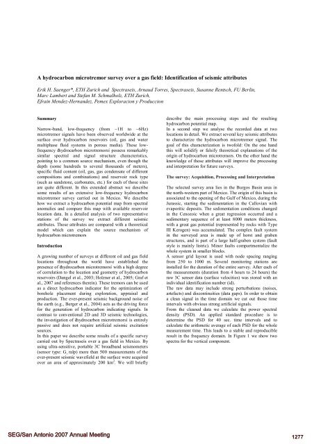
A <strong>hydrocarbon</strong> <strong>microtremor</strong> <strong>survey</strong> <strong>over</strong> a <strong>gas</strong> <strong>field</strong>: <strong>Identification</strong> <strong>of</strong> seismic attributes<br />
Erik H. Saenger*, ETH Zurich and Spectraseis, Arnaud Torres, Spectraseis, Susanne Rentsch, FU Berlin,<br />
Marc Lambert and Stefan M. Schmalholz, ETH Zurich,<br />
Efrain Mendez-Hernandez, Pemex Exploracion y Produccion<br />
Summary<br />
Narrow-band, low-frequency (from ~1H to ~6Hz)<br />
<strong>microtremor</strong> signals have been observed worldwide at the<br />
surface <strong>over</strong> <strong>hydrocarbon</strong> reservoirs (oil, <strong>gas</strong> and water<br />
multiphase fluid systems in porous media). These lowfrequency<br />
ë<strong>hydrocarbon</strong> <strong>microtremor</strong>sí possess remarkably<br />
similar spectral and signal structure characteristics,<br />
pointing to a common source mechanism, even though the<br />
depth (some hundreds to several thousands <strong>of</strong> meters),<br />
specific fluid content (oil, <strong>gas</strong>, <strong>gas</strong> condensate <strong>of</strong> different<br />
compositions and combinations) and reservoir rock type<br />
(such as sandstone, carbonates, etc.) for each <strong>of</strong> those sites<br />
are quite different. In this extended abstract we describe<br />
some results <strong>of</strong> an extensive low-frequency <strong>hydrocarbon</strong><br />
<strong>microtremor</strong> <strong>survey</strong> carried out in Mexico. We describe<br />
how we extract a <strong>hydrocarbon</strong> potential map from spectral<br />
anomalies and compare this map with available reservoir<br />
location data. In a detailed analysis <strong>of</strong> two representative<br />
stations <strong>of</strong> the <strong>survey</strong> we extract different seismic<br />
attributes. Those attributes are compared with a theoretical<br />
model which can explain the source mechanism <strong>of</strong><br />
<strong>hydrocarbon</strong> <strong>microtremor</strong>s<br />
Introduction<br />
A growing number <strong>of</strong> <strong>survey</strong>s at different oil and <strong>gas</strong> <strong>field</strong><br />
locations throughout the world have established the<br />
presence <strong>of</strong> ë<strong>hydrocarbon</strong> <strong>microtremor</strong>sí with a high degree<br />
<strong>of</strong> correlation to the location and geometry <strong>of</strong> <strong>hydrocarbon</strong><br />
reservoirs (Dangel et al., 2003; Holzner et al., 2005; Graf et<br />
al., 2007 and references therein). These tremors can be used<br />
as a direct <strong>hydrocarbon</strong> indicator for the optimization <strong>of</strong><br />
borehole placement during exploration, appraisal and<br />
production. The ever-present seismic background noise <strong>of</strong><br />
the earth (e.g., Berger et al., 2004) acts as the driving force<br />
for the generation <strong>of</strong> <strong>hydrocarbon</strong> indicating signals. In<br />
contrast to conventional 2D and 3D seismic technologies,<br />
the investigation <strong>of</strong> ë<strong>hydrocarbon</strong> <strong>microtremor</strong>sí is entirely<br />
passive and does not require artificial seismic excitation<br />
sources.<br />
In this paper we describe some results <strong>of</strong> a specific <strong>survey</strong><br />
carried out by Spectraseis <strong>over</strong> a <strong>gas</strong> <strong>field</strong> in Mexico. By<br />
using ultra-sensitive, portable 3C broadband seismometers<br />
(sensor type: G¸ ralp) more than 500 measurements <strong>of</strong> the<br />
ever-present seismic wave<strong>field</strong> at the surface were acquired<br />
<strong>over</strong> an area <strong>of</strong> approximately 200 km 2 . We will briefly<br />
SEG/San Antonio 2007 Annual Meeting<br />
describe the main processing steps and the resulting<br />
<strong>hydrocarbon</strong> potential map.<br />
In a second step we analyse the recorded data at two<br />
locations in detail. We extract several key seismic attributes<br />
to characterize the <strong>hydrocarbon</strong> <strong>microtremor</strong> signal. The<br />
goal <strong>of</strong> this characterization is tw<strong>of</strong>old: On the one hand<br />
this will solidify or falsify theoretical explanations <strong>of</strong> the<br />
origin <strong>of</strong> <strong>hydrocarbon</strong> <strong>microtremor</strong>s. On the other hand the<br />
knowledge <strong>of</strong> those attributes will improve the processing<br />
and interpretation for future <strong>survey</strong>s.<br />
The <strong>survey</strong>: Acquisition, Processing and Interpretation<br />
The selected <strong>survey</strong> area lies in the Burgos Basin area in<br />
the north-western part <strong>of</strong> Mexico. The origin <strong>of</strong> this basin is<br />
associated to the opening <strong>of</strong> the Gulf <strong>of</strong> Mexico, during the<br />
Jurassic, starting the sedimentation in the Callovian with<br />
evaporitic deposits. The sedimentation conditions changed<br />
in the Cenozoic when a great regression occurred and a<br />
sedimentary sequence <strong>of</strong> at least 8000 meters thickness,<br />
with a great <strong>gas</strong> potential (represented by rocks with Type<br />
III Kerogen) was accumulated. The complex fault system<br />
in the <strong>survey</strong>ed area is made up <strong>of</strong> horst and graben<br />
structures, and is part <strong>of</strong> a large half-graben system (fault<br />
style is mainly listric). Minor faults compartmentalize the<br />
whole system in smaller blocks.<br />
A sensor grid layout is used with node spacing ranging<br />
from 250 to 1000 m. Several monitoring stations are<br />
installed for the duration <strong>of</strong> the entire <strong>survey</strong>. After each <strong>of</strong><br />
the measurements (duration from 4 hours to 24 hours) the<br />
raw 3C sensor data (surface velocities) was stored with an<br />
individual identification number (id).<br />
The raw data may include strong perturbations (noises,<br />
artefacts) and discontinuities (data gaps). In order to obtain<br />
a clean signal in the time domain we cut out those time<br />
intervals with obvious strong artificial signals.<br />
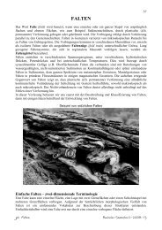
From the cleaned data we calculate the power spectral<br />
density (PSD). An applied standard procedure is to<br />
determine the PSD for 40 sec. time intervals and to<br />
calculate the arithmetic average <strong>of</strong> each PSD for the whole<br />
measurement time. This leads to a stable and reproducible<br />
result in the frequency domain. In Figure 1 we show two<br />
spectra for the vertical component.<br />
1277
Figure 1: Spectrum <strong>of</strong> the passive seismic wave<strong>field</strong><br />
(vertical surface velocities) in the frequency range from 0.5<br />
to 7.4Hz. The id 70139 was recorded <strong>over</strong> a known <strong>gas</strong><br />
<strong>field</strong>, id 70575 is <strong>over</strong> an area with no <strong>hydrocarbon</strong><br />
potential. Both locations are marked in Figure 3.<br />
One goal <strong>of</strong> the processing <strong>of</strong> <strong>hydrocarbon</strong> <strong>microtremor</strong><br />
data is to map low-frequency energy anomalies in the<br />
expected total bandwidth <strong>of</strong> the <strong>hydrocarbon</strong> <strong>microtremor</strong><br />
(i.e. between ~1 and 6Hz). We suggest to use a special<br />
integration<br />
technique: This<br />
method considers<br />
only the vertical<br />
component <strong>of</strong> the<br />
signal. The noise<br />
variations are taken<br />
into account by<br />
defining an<br />
individual minimum<br />
for each spectrum<br />
between 1 and 1.7Hz<br />
(for <strong>hydrocarbon</strong><br />
<strong>microtremor</strong>s we typically observe a minimum in this<br />
range). The integral above this level is used for determining<br />
the KTI-IZ value (see Figure 2; KTI is a project<br />
abbreviation an IZ stands for Integral <strong>of</strong> Z-component). For<br />
this Mexican <strong>gas</strong> <strong>survey</strong> we calculate the integral only<br />
between 1 and 3.7Hz because <strong>of</strong> some identified artificial<br />
noise sources above this frequency interval. As an output<br />
we receive a <strong>hydrocarbon</strong> potential map (Figure 3) based<br />
on this specific integral attribute.<br />
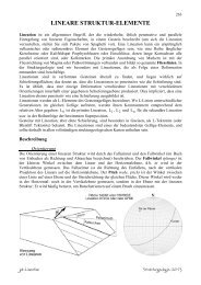
The strong KTI-IZ values are well aligned with the zone<br />
where most <strong>of</strong> the <strong>gas</strong>-producing wells are currently<br />
concentrated. This match is quite satisfactory since it shows<br />
that it was possible to detect the presence <strong>of</strong> <strong>hydrocarbon</strong>s<br />
in the most exploited part <strong>of</strong> the <strong>field</strong>.<br />
Seismic attributes <strong>of</strong> <strong>hydrocarbon</strong> <strong>microtremor</strong>s<br />
Figure 2: Green surface<br />
defines the KTI-IZ value<br />
SEG/San Antonio 2007 Annual Meeting<br />
Figure 3: Subset <strong>of</strong> a <strong>hydrocarbon</strong> potential map (3 levels<br />
<strong>of</strong> probability for the presence <strong>of</strong> <strong>gas</strong> ñ orange is the<br />
highest) together with the KTI-IZ method values<br />
(ì bubblesî showing integrated peak surfaces for Z<br />
component). Two location are marked with their<br />
identification number (id).<br />
Seismic attributes <strong>of</strong> <strong>hydrocarbon</strong> <strong>microtremor</strong>s<br />
Now we have a detailed look on the measurement-point<br />
already shown in Figure 1. The KTI-IZ value described<br />
above is one attribute to characterize <strong>hydrocarbon</strong><br />
<strong>microtremor</strong> signals. Another signature can be extracted by<br />
analyzing spectral ratios. In contrast to the well known H/V<br />
ratio method to identify soil layers we concentrate our<br />
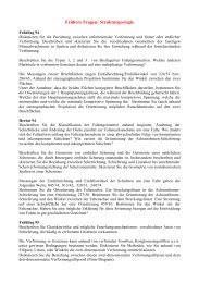
analysis on the V/H ratio (i.e. the opposite). As shown in<br />
Figure 4 one observes a peak (values significantly above 1)<br />
in this ratio in the frequency band <strong>of</strong> <strong>hydrocarbon</strong><br />
<strong>microtremor</strong>s (i.e. ca. 1..6Hz) for a station placed above<br />
<strong>hydrocarbon</strong>s. For details how we calculate this ratio refer<br />
to Lambert et al. (2006).<br />
1278
Figure 4: V/H ratio <strong>of</strong> the passive seismic wave<strong>field</strong> in the<br />
frequency range from 0.5 to 10Hz. The id 70139 was<br />
recorded <strong>over</strong> a known <strong>gas</strong> <strong>field</strong> (left hand side), id 70575<br />
is <strong>over</strong> an area with no <strong>hydrocarbon</strong> potential. The dashed<br />
line indicates a value <strong>of</strong> V/H=1.<br />
It is also possible to perform a polarization analysis <strong>of</strong> the<br />
recorded <strong>microtremor</strong> data. The first step in this procedure<br />
is to bandpass-filter the 3C-data in the time domain. We<br />
apply a zero-phase filter which cuts out the frequencies<br />
from 1Hz to 3.7Hz for further analysis. In this work, the<br />
analysis <strong>of</strong> the polarization behavior <strong>over</strong> 40sec.-time<br />
intervals was adapted from Jurkevics (1988). Considering<br />
any time interval <strong>of</strong> three-component data ux, uy and uz<br />
containing N time samples auto- and cross-variances can be<br />
obtained with:<br />
C<br />
⎡ 1<br />
⎢<br />
⎣ N<br />
N<br />
= ∑<br />
s=<br />
Seismic attributes <strong>of</strong> <strong>hydrocarbon</strong> <strong>microtremor</strong>s<br />
⎤<br />
ui(<br />
s)<br />
u j ( s)<br />
⎥<br />
⎦<br />
ij<br />
1<br />
where i and j represent the component index x, y, z and s is<br />
the index variable for a time sample. The 3◊3 covariance<br />
matrix<br />
⎛C<br />
⎜<br />
C = ⎜C<br />
⎜<br />
⎝C<br />
xx<br />
xy<br />
xz<br />
C<br />
C<br />
C<br />
xy<br />
yy<br />
yz<br />
C<br />
C<br />
C<br />
xz<br />
yz<br />
zz<br />
⎞<br />
⎟<br />
⎟<br />
⎟<br />
⎠<br />
is real and symmetric and represents a polarization ellipsoid<br />
with best fit to the data. The principal axis <strong>of</strong> this ellipsoid<br />
can be obtained by solving C for its eigenvalues λ1 7λ2 7λ3<br />
and eigenvectors p1, p2, p3:<br />
( C − λ I ) p = 0<br />
where I is the identity matrix.<br />
The parameter called rectilinearity L, sometimes also called<br />
linearity, relates the magnitudes <strong>of</strong> the intermediate and<br />
smallest eigenvalue to the largest eigenvalue<br />
⎛ λ2<br />
+ λ3<br />
⎞<br />
L = 1−<br />
⎜ ,<br />
2 ⎟<br />
⎝ λ1<br />
⎠<br />
and measures the degree <strong>of</strong> how linear the incoming<br />
wave<strong>field</strong> is polarized. It yields values between zero and<br />
one. The other two polarization parameters describe the<br />
SEG/San Antonio 2007 Annual Meeting<br />
orientation <strong>of</strong> the largest eigenvector p1 = (p1(x), p1(y),<br />
p1(z)) in dip and azimuth. The dip can be calculated with<br />
⎛<br />
φ = arctan⎜<br />
⎜<br />
⎝<br />
p ( x)<br />
1<br />
p ( z)<br />
1<br />
2<br />
+ p ( y)<br />
and is zero for horizontal polarization and is defined<br />
positive in positive z-direction. The azimuth is specified as<br />
⎛ p ⎞ 1(<br />
y)<br />
θ = arctan ⎜<br />
⎟<br />
⎝ p1(<br />
x)<br />
⎠<br />
and measured positive counterclockwise (ccw) from the<br />
positive x-axis. In addition we analyse the strength <strong>of</strong> the<br />
signal which is given by the eigenwert λ1. All four<br />
attributes are illustrated in Figure 5.<br />
Figure 5: Polarization parameter sketch. Reliability <strong>of</strong> dip<br />
and azimuth. Left hand side: high rectilinearity and<br />
medium dip, Right hand side: low rectilinearity and<br />
relatively high dip. The length <strong>of</strong> the red arrow is given by<br />
the largest eigenvalue λ1, further refered as the strength <strong>of</strong><br />
the signal.<br />
In Figure 6 and 7 we apply the analysis explained above to<br />
our <strong>microtremor</strong> data <strong>of</strong> station id 70139 and 70575 with<br />
high and low <strong>hydrocarbon</strong> potential, respectively. It is clear<br />
that we have on the surface a complicated mixture <strong>of</strong><br />
different wave types with different origins. However, we<br />
have identified very stable trends in the selected <strong>gas</strong> <strong>survey</strong><br />
regarding the attributes dip, azimuth, rectilinearity and<br />
strength in the <strong>hydrocarbon</strong> <strong>microtremor</strong> frequency range<br />
(i.e. 1..3.7Hz). We summarize our observations as follows:<br />
Above a reservoir (station id 70139):<br />
- Dip: Stable high value (≥80 o ) directly above the<br />
reservoir (Figure 7, top, left hand side).<br />
- Strength: Varying, but present <strong>over</strong> the whole<br />
measure period.<br />
- Rectilinearity: Relative high and relatively stable<br />
and somehow correlated with the strength<br />
- Azimuth: Strongly varying, as expected for such<br />
high dip values.<br />
1<br />
2<br />
⎞<br />
⎟<br />
⎟<br />
⎠<br />
1279
For a measure point with low <strong>hydrocarbon</strong> potential<br />
(station id 70575):<br />
- Dip: Stable low value (≈20 o , Figure 7, top, left hand<br />
side).<br />
- Strength: Relatively low with some spikes.<br />
- Rectilinearity: Lower in comparison with the values<br />
observed above a <strong>hydrocarbon</strong> reservoir.<br />
- Azimuth: Relatively stable; maybe points to an<br />
artificial noise source.<br />
Figure 6: Time variations <strong>of</strong> dip (φ), strength (λ1),<br />
rectilinearity (L) and azimuth (θ) for bandpass-filtered<br />
data (1..3.7Hz) from station id 70139 (High <strong>hydrocarbon</strong><br />
potential). The time unit on the horizontal axes is periods <strong>of</strong><br />
40sec. The solid line represents the value using data <strong>of</strong> the<br />
whole time period.<br />
Figure 7: Same as Figure 6 but for station id 70575 (Low<br />
Hydrocarbon potential)<br />
A theoretical model based on observed attributes<br />
In Graf et al. (2007) we discuss some possible origins <strong>of</strong><br />
<strong>hydrocarbon</strong> <strong>microtremor</strong>s. Based on the seismic attributes<br />
identified in this paper we suggest the following theoretical<br />
model. The driven sources are ocean waves interacting with<br />
the coast structure. They produce the so-called ocean-wave<br />
SEG/San Antonio 2007 Annual Meeting<br />
Seismic attributes <strong>of</strong> <strong>hydrocarbon</strong> <strong>microtremor</strong>s<br />
peak around 0.1Hz in the seismic background noise (e.g.<br />
Berger et al. 2004) which can be observed on all locations<br />
around the world. Those surface waves propagate through<br />
whole continents and can be used for determining seismic<br />
velocities down to a depth <strong>of</strong> 20km (e.g. Shapiro et al.<br />
2005). Interestingly, Rayleigh waves around 0.1Hz<br />
oscillate at reservoir depth (deeper than ≈500m) mainly in<br />
vertical direction (e.g. Aki and Richards 2002). By a<br />
complex resonant amplification effect (see Graf et al. 2007<br />
and references therein) with the <strong>hydrocarbon</strong> reservoir the<br />
<strong>microtremor</strong> itself produce a radiation pattern as shown in<br />
Figure 8. Directly above the reservoir one observe mainly<br />
P-waves. This is consistent with the following observations<br />
at id 70139 <strong>of</strong> the selected <strong>gas</strong> reservoir <strong>survey</strong>: Strong<br />
anomaly in the vertical component (Figure 1), a peak in the<br />
V/H-ratio (Figure 4), a constant high dip with a relatively<br />
high rectilinearity and an non-vanishing strength as shown<br />
in Figure 6.<br />
Figure 8: A model which explains the observed seismic<br />
attributes.<br />
Conclusions<br />
We have described a low-frequency <strong>hydrocarbon</strong><br />
<strong>microtremor</strong> <strong>survey</strong> <strong>over</strong> a <strong>gas</strong> <strong>field</strong> in Mexico. As in<br />
previous case studies (Graf et al. 2007 and references<br />
therein) we observe a high correlation <strong>of</strong> the <strong>hydrocarbon</strong><br />
<strong>microtremor</strong> signal with the known location <strong>of</strong> the <strong>gas</strong><br />
reservoir. With a deeper analysis we have indentified and<br />
specified different seismic attributes <strong>of</strong> the signal: KTI-IZ<br />
value, V/H-signal, dip, rectilinearity and strength. Based on<br />
those attributes we propose a model <strong>of</strong> the origin <strong>of</strong> the<br />
described LF-signal.<br />
Acknowledgements<br />
We are gratefully to Pemex and Spectraseis for the<br />
permission to publish the data. Swiss KTI-program has c<strong>of</strong>inanced<br />
this work<br />
1280
EDITED REFERENCES<br />
Note: This reference list is a copy-edited version <strong>of</strong> the reference list submitted by the author. Reference lists for the 2007<br />
SEG Technical Program Expanded Abstracts have been copy edited so that references provided with the online metadata for<br />
each paper will achieve a high degree <strong>of</strong> linking to cited sources that appear on the Web.<br />
REFERENCES<br />
Aki, K., and Richards, P. G., 2002, Quantitative seismology, 2nd ed: University Science Books.<br />
Berger, J., P. Davis, and G. Ekstrom, 2004, Ambient earth noise: A <strong>survey</strong> <strong>of</strong> the global seismograph network: Journal<br />
Geophysical Research, 109, B11307; http://dx.doi.org/10.1029/2004JB003408.<br />
Dangel, S., M. E. Schaepman, E. P.Stoll, R. Carniel, O. Barzandji, E. D. Rode, and J. M. Singer, 2003, Phenomenology <strong>of</strong><br />
tremor-like signals observed <strong>over</strong> <strong>hydrocarbon</strong> reservoirs: Journal <strong>of</strong> Volcanology and Geothermal Research 128, 135–<br />
158.<br />
Graf, R., S. M. Schmalholz, Y. Podladchikov, and E. H. Saenger, 2007, Passive low frequency spectral analysis: Exploring a new<br />
<strong>field</strong> in geophysics: World Oil, 228, 47–52.<br />
Holzner, R., P. Eschle, H. Zuercher, M. Lambert, R. Graf, S. Dangel, and P. F. Meier, 2005, Applying <strong>microtremor</strong> analysis to<br />
identify <strong>hydrocarbon</strong> reservoirs: First Break, 23, 41–49.<br />
Jurkevics, A., 1988, Polarization analysis <strong>of</strong> three-component array data: Bulletin <strong>of</strong> the Seismological Society <strong>of</strong> America, 78,<br />
1725–1743.<br />
Lambert, M., B. Steiner, S. M. Schmalholz, R. Holzner, and E. H. Saenger, 2006, S<strong>of</strong>t soil amplification <strong>of</strong> ambient seismic noise<br />
– <strong>field</strong> measurements and numerical modeling <strong>of</strong> H/V ratios: Passive Seismic Workshop, EAGE, A10.<br />
Shapiro, N. M., M. Campillo, L.Stehly, and M. Ritzwoller, 2005, High resolution surface wave tomography from ambient<br />
seismic noise: Science, 307, 1615–1618.<br />
SEG/San Antonio 2007 Annual Meeting<br />
1281