van den Berg et al., 2005, Earth Planetary Science Letters.

More documents

Recommendations

Info

264 A.P. van den Berg et al. / Physics of the Earth and Planetary Interiors 149 (2005) 259–278 ary q C described by the ordinary differential equation (Steinbach et al., 1993) dT C dt A = − q C (t) (8) ρ C c PC V C where A is the area of the core–mantle boundary surface and C C = ρ C c PC V C is the total heat capacity of the core. The core heat capacity is expressed as a fraction X of the mantle heat capacity C M , resulting in an O.D.E. for T C (t): dT C dt = − 1 Xρc p h q C(t) (9) where ρ and c p are the mantle values of density and heat capacity. Parameter values are given in Table 1. At each time step T C is updated by integrating (9), using the average heatflow value q C , computed from the finite element solution for the mantle temperature field. This is done by forward extrapolation in time of the heat flux in an Euler type scheme. The updated uniform core temperature is then taken as a time dependent boundary condition for the finite element computation of the mantle temperature in the next time step, so T CMB (t) = T C (t) in (9). We note that analytical asymptotic methods (Solomatov and Zharkov, 1990) for treating thermal history, though capable of handling variable viscosity, may be hard-pressed to apply in the case of variable thermal conductivity. 3. Results A comparison of a series of temperature snapshots for typical secular cooling runs for two different values of the T CMB (0) = 3273 and 4273 K is shown in Fig. 2. The snapshots represent a time span of about the age of the Earth, illustrating the effects of different initial T CMB (0), showing faster cooling for the hotter initial temperature case. In previous work we have investigated the impact of variable conductivity on the secular cooling of the convecting mantle, restricted to isoviscous models (van den Berg and Yuen, 2002) and to models with temperature dependence of the viscosity limited to around 1000 (van den Berg et al., 2004). Here we consider models including pressure and temperature dependent viscosity given by (7) with a higher value of the temperature dependence. In contrast to previous work we also focus on the opposite role of the different heat transport mechanisms (phonons versus photons) in the composite conductivity model. Finally we introduce here thermal coupling between the convecting mantle and a thermal reservoir representing the core. Photon conductivity is likely to be dominant in the lower mantle and hence important for thermal core/mantle coupling. Phonon conductivity is suppressed by the 1/T temperature dependence. The effect of varying η T on the overall cooling history of the coupled mantle and core system is presented in Figs. 3 and 4. The cooling curves in Fig. 3, show the volume averaged temperature of the mantle, comparing also the variable conductivity cases with the corresponding constant conductivity cases. The corresponding constant conductivity cases have the same surface conductivity value as the variable conductivity cases. For the conductivity model with f = 1 this also corresponds to an approximately similar value of the volume average conductivity. This was also shown in previous work, Fig. 7 of van den Berg and Yuen (2002). The main feature of the results shown in Figs. 3 and 4 is a similar cooling delay of the variable conductivity models with respect to the corresponding constant conductivity models. This amounts to an accumulated delay time of almost two billion years at a model time of 4.5 Gyr. These results indicate that the delay we found earlier in secular cooling in isoviscous models with variable conductivity is a robust phenomenon, also in models including variable viscosity. The results also show that the trend in the cooling rate, for increasing η T , is non-monotonic. It appears that cooling is slightly slower for η T = 3 × 10 3 (Fig. 3b) than for η T = 3 × 10 2 (Fig. 3a). Increasing the temperature to η T = 3 × 10 4 the cooling rate increases also (Fig. 3c). This non-monotonic trend is the same for constant conductivity models represented by the dashed curves. The small difference in the overall cooling behavior between the three contrasting viscosity cases is surprising inview of the significant difference of the interior viscosity shown for these cases shown in Fig. 4. It appears from these results that one cannot simply apply the temperature dependence of the viscosity to predict an increased cooling rate for increasing η T . The pressure dependence of the viscosity complicates the details of the resulting temperature distribution which feeds back into the viscosity, resulting in this non-monotonic behavior.
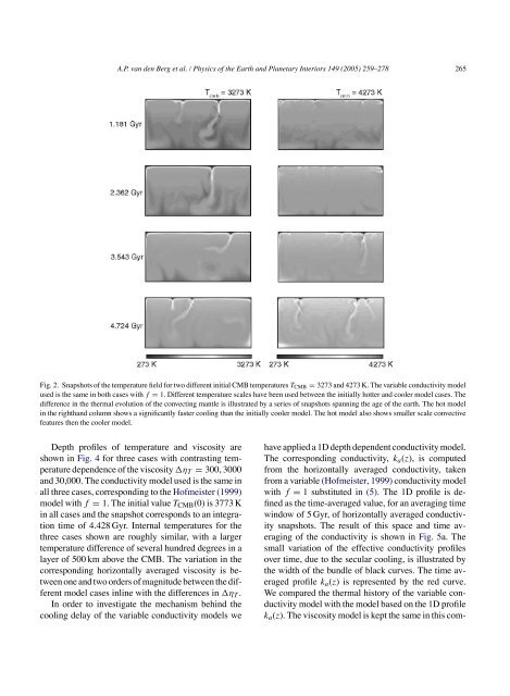
A.P. van den Berg et al. / Physics of the Earth and Planetary Interiors 149 (2005) 259–278 265 Fig. 2. Snapshots of the temperature field for two different initial CMB temperatures T CMB = 3273 and 4273 K. The variable conductivity model used is the same in both cases with f = 1. Different temperature scales have been used between the initially hotter and cooler model cases. The difference in the thermal evolution of the convecting mantle is illustrated by a series of snapshots spanning the age of the earth. The hot model in the righthand column shows a significantly faster cooling than the initially cooler model. The hot model also shows smaller scale convective features then the cooler model. Depth profiles of temperature and viscosity are shown in Fig. 4 for three cases with contrasting temperature dependence of the viscosity η T = 300, 3000 and 30,000. The conductivity model used is the same in all three cases, corresponding to the Hofmeister (1999) model with f = 1. The initial value T CMB (0) is 3773 K in all cases and the snapshot corresponds to an integration time of 4.428 Gyr. Internal temperatures for the three cases shown are roughly similar, with a larger temperature difference of several hundred degrees in a layer of 500 km above the CMB. The variation in the corresponding horizontally averaged viscosity is between one and two orders of magnitude between the different model cases inline with the differences in η T . In order to investigate the mechanism behind the cooling delay of the variable conductivity models we have applied a 1D depth dependent conductivity model. The corresponding conductivity, k a (z), is computed from the horizontally averaged conductivity, taken from a variable (Hofmeister, 1999) conductivity model with f = 1 substituted in (5). The 1D profile is defined as the time-averaged value, for an averaging time window of 5 Gyr, of horizontally averaged conductivity snapshots. The result of this space and time averaging of the conductivity is shown in Fig. 5a. The small variation of the effective conductivity profiles over time, due to the secular cooling, is illustrated by the width of the bundle of black curves. The time averaged profile k a (z) is represented by the red curve. We compared the thermal history of the variable conductivity model with the model based on the 1D profile k a (z). The viscosity model is kept the same in this com-
Page 1 and 2: Physics of the Earth and Planetary
Page 3 and 4: A.P. van den Berg et al. / Physics
Page 5: A.P. van den Berg et al. / Physics

van den Berg et al., 2005, Earth Planetary Science Letters.

You also want an ePaper? Increase the reach of your titles

Delete template?

Save as template?