2. Average rate of change
2. Average rate of change
2. Average rate of change

You also want an ePaper? Increase the reach of your titles
YUMPU automatically turns print PDFs into web optimized ePapers that Google loves.
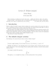
Lecture 2: Rates <strong>of</strong> <strong>change</strong><br />
Nathan Pflueger<br />
11 September 2013<br />
1 Introduction<br />
Calculus was initially developed in large part to study the motion <strong>of</strong> planets and other physical problems.<br />
The basic insight behind Newton’s laws <strong>of</strong> motion is that the motion <strong>of</strong> physical objects is best describing<br />
by talking about their velocity and acceleration; calculus provided the vocabulary and logical apparatus to<br />
do this. Velocity is the most familiar example <strong>of</strong> a <strong>rate</strong> <strong>of</strong> <strong>change</strong>, while accelerations is the <strong>rate</strong> <strong>of</strong> <strong>change</strong><br />
<strong>of</strong> velocity.<br />
This lecture begins a basic, informal discussion about what we mean when we say <strong>rate</strong> <strong>of</strong> <strong>change</strong>. The<br />
basic idea is simple: it tells how much a quantity (like distance traveled along a road) will <strong>change</strong> in a given<br />
period <strong>of</strong> time. We will see how this concept graphically as a secant line. The trouble is that objects don’t<br />
keep moving at a steady speed forever, so we must think about what a <strong>rate</strong> <strong>of</strong> <strong>change</strong> (like velocity) can<br />
mean at a particular instant, not over a period <strong>of</strong> time. Graphically this corresponds to the idea <strong>of</strong> a tangent<br />
line, which is a sort <strong>of</strong> idealized secant line. This will lead into a discussion <strong>of</strong> limits in the next lecture,<br />
where we will describe the modern way to make this transition (secant to tangent) a bit more precise.<br />
The reference for todays material is section <strong>2.</strong>1 <strong>of</strong> Stewart.<br />
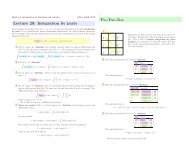
2 Example: rising water level in a flask<br />
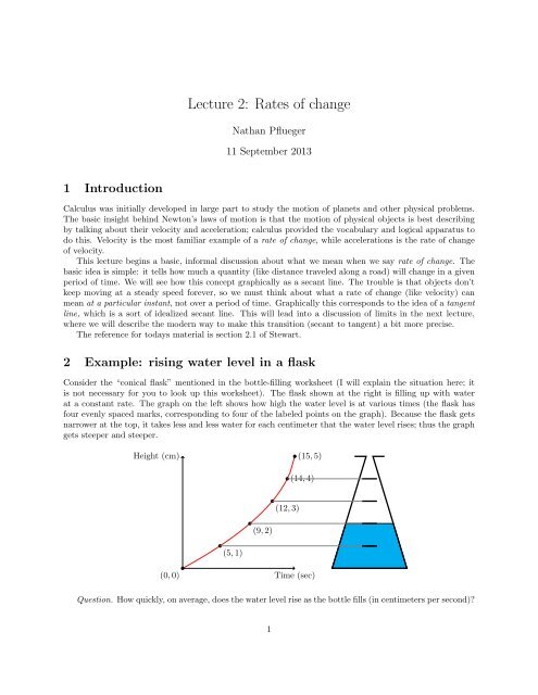
Consider the “conical flask” mentioned in the bottle-filling worksheet (I will explain the situation here; it<br />
is not necessary for you to look up this worksheet). The flask shown at the right is filling up with water<br />
at a constant <strong>rate</strong>. The graph on the left shows how high the water level is at various times (the flask has<br />
four evenly spaced marks, corresponding to four <strong>of</strong> the labeled points on the graph). Because the flask gets<br />
narrower at the top, it takes less and less water for each centimeter that the water level rises; thus the graph<br />
gets steeper and steeper.<br />
Height (cm)<br />
(15, 5)<br />
(14, 4)<br />
(12, 3)<br />
(9, 2)<br />
(5, 1)<br />
(0, 0)<br />
Time (sec)<br />
Question. How quickly, on average, does the water level rise as the bottle fills (in centimeters per second)?<br />
1
Answer. The water level rises a total <strong>of</strong> 5cm, over the course <strong>of</strong> 15 seconds. Therefore the average <strong>rate</strong><br />
that the water rises is 5cm<br />
15s<br />
≈ 0.333cm/s.<br />
Question. How quickly (on average) is the height rising as it rises from the bottom <strong>of</strong> the bottle to the<br />
first mark (1 cm up)? From the first mark to the second? The second to the third? The third to the fourth?<br />
From the fourth to the top <strong>of</strong> the bottle?<br />
Answer. In each case, the average <strong>rate</strong> that the water rises is the total rise (in centimeters) divided by<br />
the time (in seconds). Therefore these are:<br />
• From the bottom to the first mark:<br />
1cm<br />
5s<br />
= 0.200cm/s.<br />
• From the first mark to the second:<br />
• From the second mark to the third:<br />
(2−1)cm<br />
(9−5)s<br />
(3−2)cm<br />
(12−9)s<br />
= 0.250cm/s.<br />
≈ 0.333cm/s.<br />
• From the third mark to the fourth:<br />
• From the fourth mark to the top:<br />
(4−3)cm<br />
(14−12)s = 0.500cm/s.<br />
(5−4)cm<br />
(15−14)s = 1.000cm/s.<br />
As we could guess from looking at the picture, the <strong>rate</strong> that the height goes up is increasing as the bottle<br />
fills. It increases gently at first and then begins to increase dramatically at the end.<br />
Visually, these <strong>rate</strong>s <strong>of</strong> increase correspond to the slopes <strong>of</strong> the secant lines joining adjacent pairs <strong>of</strong><br />
points. Note that in this pictures, the x and y axes use slightly different scales; this is why the line look<br />
steeper than you would think from the numbers.<br />
0.200cm/s 0.250cm/s 0.333cm/s 0.500cm/s 1.000cm/s<br />
3 Example: a bicycle speedometer<br />
Many bicycle speedometers work in the following way: a small magnet is attached to one <strong>of</strong> the spokes <strong>of</strong><br />
a wheel. Every time the wheel makes a full revolution, a small sensor detects the magnet passing by. How<br />
can this device be used to measure the speed the bicycle is traveling?<br />
This device can measure speed because it knows the two main pieces <strong>of</strong> information: the number <strong>of</strong><br />
meters traveled, and the amount <strong>of</strong> time it took to travel them. The distance traveled is just the number<br />
<strong>of</strong> times the magnet passed by multiplied by the circumference <strong>of</strong> the wheel (since this is how far the bike<br />
travels with each revolution). The device can determine the time it takes to travel this distance by measuring<br />
the time between each moment it detects the magnet.<br />
Suppose that the bicycle wheel has circumference 2 meters. Then the speedometer, in effect, can tell<br />
how much time has passed every time the bicycle travels another two meters. Suppose that it records the<br />
following data.<br />
Time elapsed (seconds) 0.00 <strong>2.</strong>0 3.6 4.8 5.6 6.0<br />
Distance traveled (meters) 0 2 4 6 8 10<br />
Question. At what speed does the bicycle travel these 10 meters, on average? How fast is it traveling for<br />
the first 2 meters? The second 2 meters? The third, fourth, and fifth?<br />
Answer. The bicycle travels the first 2 meters at an average <strong>of</strong> 2m<br />
2s<br />
= 1m/s (this is approximately<br />
<strong>2.</strong>24milesperhour). The second two meters are completed at 2m<br />
1.6s<br />
= 1.25m/s. The third are completed at<br />
2
2m<br />
1.2s<br />
at 2m<br />
0.4s<br />
2m<br />
≈ 1.67m/s. The fourth two meters are completed at<br />
0.8s<br />
= <strong>2.</strong>50m/s. The last two meters are completed<br />
= 5m/s, or about 11 miles per hour.<br />
Notice that this example is essentially identical to the previous example. All I’ve done is<br />
multiplied the x values by 0.4 and the y values by 2 to get more realistic figures for this situation.<br />
Question. How fast is the bicycle traveling after exactly 2 seconds?<br />
Distance (m)<br />
(0, 0)<br />
(2, 2)<br />
(6, 10)<br />
(5.6, 8)<br />
(4.8, 4)<br />
(3.6, 4)<br />
Time (sec)<br />
Answer. The tricky thing about this question is that we’re no longer asking for an average – we want to<br />
know how fast the bicycle is traveling at that instant. And unfortunately the answer is: the device can’t tell<br />
precisely. All it knows is how <strong>of</strong>ten the magnet goes all the way around. However, we can get a pretty good<br />
guess: we know that the instant when 3 seconds has passed lies somewhere in between the moment when<br />
the wheel made one revolution (2 seconds in) and the moment when the wheel made two revolutions (3.6<br />
seconds in). From the previous problem, we know that the average speed in this interval was 1.25 m/s.<br />
This is the slope <strong>of</strong> the tangent line between the two sensor readings mentioned.<br />
Distance (m)<br />
(0, 0)<br />
(2, 2)<br />
(6, 10)<br />
(5.6, 8)<br />
(4.8, 4)<br />
(3.6, 4)<br />
Time (sec)<br />
From the picture, we see that the secant line between the corresponding points on the graph is a very<br />
good approximation <strong>of</strong> the function in this range, so its slope is a very good guess at the instantaneous <strong>rate</strong><br />
<strong>of</strong> <strong>change</strong>. To get a better guess would require either a more precise measuring device (for example, magnets<br />
on more spokes <strong>of</strong> the wheel) or some assumptions about how quickly the bicycle accele<strong>rate</strong>s during this<br />
interval.<br />
To even be able to tell that the secant line is not a perfect approximation requires zooming in on this<br />
graph, as shown below. Here, both the secant line we’ve used to approximate the speed, and the tangent<br />
line whose slope is the true speed, are shown. The difference in their slopes is clearly very small.<br />
3
(3.6, 4)<br />
(3, ?)<br />
(2, 2)<br />
Question to think about. Is this sort <strong>of</strong> bike speedometer more accu<strong>rate</strong> at high speeds or low speeds?<br />
Why?<br />
4 Secant lines and tangent lines<br />
As we’ve seen in the last two examples, the concept <strong>of</strong> average <strong>rate</strong> <strong>of</strong> <strong>change</strong>, namely<br />
Avg. <strong>rate</strong> <strong>of</strong> <strong>change</strong> =<br />
total <strong>change</strong><br />
total time elapsed<br />
has a geometric counterpart: the slope <strong>of</strong> a secant line. This is illust<strong>rate</strong>d in the following picture. A<br />
secant line just means a line passing through two chosen points on a graph.<br />
total <strong>change</strong><br />
total time elapsed<br />
A slightly more slippery concept is the instantaneous <strong>rate</strong> <strong>of</strong> <strong>change</strong>. It is remarkably hard to define what<br />
we mean by this term. But we have all watched the speedometer on a car: at any moment, it is pointing<br />
somewhere. Where it’s pointing, as far as we are concerned, is the speed that the car is currently, at that<br />
very instant, traveling.<br />
The graphical equivalent <strong>of</strong> instantaneous <strong>rate</strong> <strong>of</strong> <strong>change</strong> is the tangent line. One way to understand the<br />
tangent line is purely visually: it is the line that perfectly kisses the graph at a chosen point 1 .<br />
1 A use the word kisses here partly for historical reasons: sometimes the tangent line is called an osculating line, from the<br />
latin word osculum, for kiss.<br />
4
Why should such a line, however nicely it kisses the graph, tell something like an instantaneous <strong>rate</strong><br />
<strong>of</strong> <strong>change</strong>? One explanation is that it shows where the graph would go if it would just settle down, stop<br />
turning, and travel straight. The slope, then, is the average <strong>rate</strong> <strong>of</strong> <strong>change</strong> after the points where the graph<br />
has started moving straight.<br />
Another way to understand the tangent line is that it is a sort <strong>of</strong> idealized secant line. We like secant<br />
lines better if the two points are very close together, so that we can measure speed clearly without too much<br />
acceleration happening. There is no perfect secant line, because the two points are always a little apart. But<br />
we can try harder and harder, and draw closer and closer. The tangent line is a sort <strong>of</strong> Platonic ideal: the<br />
secant line that God would draw, where the two points are so close together that they are actually the same<br />
point.<br />
5
Example 4.1. What is the slope <strong>of</strong> the tangent line to the graph <strong>of</strong> y = −x 2 + 12x − 11 at (1, 0)?<br />
Solution. Begin by considering any other point (x, y) on the graph, and find the slope <strong>of</strong> the secant line<br />
through (1, 0) and (x, y). The slope <strong>of</strong> this line is rise run = y−0<br />
x−1<br />
. The following table shows some sample values,<br />
with x getting closer and closer to 1.<br />
x y slope<br />
9−0<br />
2 9<br />
2−1 = 9<br />
0.99<br />
1.1 0.99<br />
0.1 = 9.9<br />
0.0999<br />
1.01 0.0999<br />
0.01 = 9.99<br />
0.009999<br />
1.001 0.009999<br />
0.001<br />
= 9.999<br />
0<br />
1 0<br />
0 = ???<br />
−0.010001<br />
0.999 −0.010001<br />
−0.001<br />
= 10.001<br />
−0.1001<br />
0.99 −0.1001<br />
−0.01 = 10.01<br />
−1.01<br />
0.9 −1.01<br />
−0.1 = 10.1<br />
−5.25<br />
0.5 −5.25<br />
−0.5 = 10.5<br />
The pattern is clear: for values <strong>of</strong> x very close to 1, the secant line from (1, 0) to (x, y) has slope very<br />
close to 10. But we can’t quite move the second point “right on top <strong>of</strong>” the first point, since the slope would<br />
then appear to be 0/0, which is undefined.<br />
In this case, however, we can see fairly easily why the slope gets close to 10 in such a regular way. The<br />
value <strong>of</strong> the slope, for any value <strong>of</strong> x other than 1, is given by<br />
6
ise<br />
run<br />
=<br />
y<br />
x − 1<br />
= −x2 + 12x − 11<br />
x − 1<br />
(x − 1)(11 − x)<br />
=<br />
x − 1<br />
= 11 − x.<br />
Now this is an expression that we can put 1 into very easily, to obtain 10. This suggests that if we could<br />
take a secant line “from the point to itself,” the slope would be 10. And indeed, this is the slope <strong>of</strong> the<br />
tangent line.<br />
The next lecture discusses the usual formalism for doing problems like the one above.<br />
5 Appendix: The other use <strong>of</strong> the words “secant” and “tangent”<br />
Note. Whenever a section is labeled as an appendix in these notes, it is completely optional and included<br />
just for those who may be interested. Of course, all <strong>of</strong> these notes are optional reading, but the appendices<br />
in particular are not about anything that will be mentioned in homework or exams.<br />
In class, a student asked about what the terms secant and tangent (as we use them here) have to do with<br />
their usual usage, namely the following trigonometric functions.<br />
secant function sec θ = 1<br />
cos θ<br />
tangent function tan θ = sin θ<br />
cos θ<br />
The answer is that the two things (secant/tangent lines, and the secant/tangent functions) are rooted<br />
in the same etymology, but don’t have any substantive relationship that you need to worry about. The<br />
common etymology comes from the following diagram.<br />
sec θ<br />
tan θ<br />
θ<br />
1<br />
In the early days <strong>of</strong> trigonometry, functions were defined very explicitly in terms <strong>of</strong> lengths <strong>of</strong> line segments<br />
in figures. The functions sec θ and tan θ were defined like in the figure above: two lines are drawn to a circle<br />
<strong>of</strong> radius 1: one <strong>of</strong> them is a tangent line (blue), and one is a secant line (red). The angle θ is as shown.<br />
Then the quantities sec θ and tan θ are defined as the two lengths shown.<br />
So the common name simply comes from the fact that the secant function is defined in terms <strong>of</strong> a segment<br />
<strong>of</strong> a secant line to a circle, while the tangent function is defined to be a segment <strong>of</strong> a tangent line.<br />
7