Paper - Computer Graphics and Multimedia - RWTH Aachen ...
Paper - Computer Graphics and Multimedia - RWTH Aachen ...
Paper - Computer Graphics and Multimedia - RWTH Aachen ...

You also want an ePaper? Increase the reach of your titles
YUMPU automatically turns print PDFs into web optimized ePapers that Google loves.
Spectral Quadrangulation with Orientation <strong>and</strong> Alignment Control<br />
Jin Huang † Muyang Zhang Jin Ma Xinguo Liu † Leif Kobbelt ∗ Hujun Bao †<br />
State Key Lab. of CAD&CG, Zhejiang University<br />
∗ <strong>RWTH</strong> <strong>Aachen</strong> University<br />
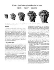
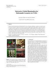
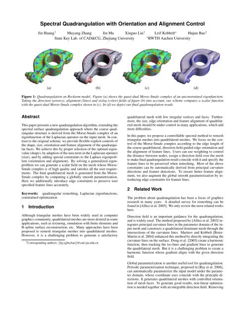
(a) (b) (c) (d)<br />
Figure 1: Quadrangulation on Rockarm model. Figure (a) shows the quasi-dual Morse-Smale complex of an unconstrained eigenfunction.<br />
Taking the direction (arrows), alignment (lines) <strong>and</strong> sizing (color) fields of figure (b) into account, our scheme computes a scalar function<br />
with the quasi-dual Morse-Smale complex shown in (c). In (d) we depict our final quadrangulation result.<br />
Abstract<br />
This paper presents a new quadrangulation algorithm, extending the<br />
spectral surface quadrangulation approach where the coarse quadrangular<br />
structure is derived from the Morse-Smale complex of an<br />
eigenfunction of the Laplacian operator on the input mesh. In contrast<br />
to the original scheme, we provide flexible explicit controls of<br />
the shape, size, orientation <strong>and</strong> feature alignment of the quadrangular<br />
faces. We achieve this by proper selection of the optimal eigenvalue<br />
(shape), by adaption of the area term in the Laplacian operator<br />
(size), <strong>and</strong> by adding special constraints to the Laplace eigenproblem<br />
(orientation <strong>and</strong> alignment). By solving a generalized eigenproblem<br />
we can generate a scalar field on the mesh whose Morse-<br />
Smale complex is of high quality <strong>and</strong> satisfies all the user requirements.<br />
The final quadrilateral mesh is generated from the Morse-<br />
Smale complex by computing a globally smooth parametrization.<br />
Here we additionally introduce edge constraints to preserve user<br />
specified feature lines accurately.<br />
Keywords: quadrangular remeshing, Laplacian eigenfunctions,<br />
constrained optimization<br />
1 Introduction<br />
Although triangular meshes have been widely used in computer<br />
graphics community, quadrilateral meshes are more desired in some<br />
applications, such as texturing, simulation with finite elements <strong>and</strong><br />
B-spline surface reconstruction, etc. Many approaches have been<br />
proposed to remesh triangular meshes into quadrilateral meshes.<br />
However, it is a challenging problem to generate a satisfactory<br />
† Corresponding authors: {hj,xgliu,bao}@cad.zju.edu.cn<br />
quadrilateral mesh with few irregular vertices <strong>and</strong> faces. Furthermore,<br />
the size, edge orientation <strong>and</strong> feature alignment of quadrilateral<br />
mesh should be under control in many applications, which add<br />
more difficulties.<br />
In this paper, we propose a controllable spectral method to remesh<br />
triangular meshes into quadrilateral meshes. We focus on the control<br />
of the Morse-Smale complex according to the edge length of<br />
the coarse quadrilateral, direction field guided edge orientation <strong>and</strong><br />
the alignment of feature lines. Users can use weighting to control<br />
the distance between nodes, assign a direction field over the mesh<br />
to make final quadrangulation result coincide with it <strong>and</strong> specify the<br />
feature lines to be preserved when remeshing. Most of the above<br />
constraints can be automatically derived from principal curvature<br />
directions <strong>and</strong> feature detections. To ensure better feature alignment,<br />
we also augment the global smooth parameterization by introducing<br />
edge constraints for feature lines.<br />
2 Related Work<br />
The problem about quadrangulation has been a focus of graphics<br />
research in many years. A detailed survey for remeshing can be<br />
found in [Alliez et al. 2005]. We only review the most related works<br />
here.<br />
Direction field is an important guidance for the quadrangulation,<br />
<strong>and</strong> is widely used. The method proposed by [Alliez et al. 2003] integrates<br />
principal curvature lines in the parameter domain of the input<br />
mesh <strong>and</strong> constructs a quadrilateral dominant mesh through the<br />
intersections of the curvature lines. Marinov <strong>and</strong> Kobbelt [Boier-<br />
Martin et al. 2004] enhanced this method by directly integrating the<br />
curvature lines on the surface. Dong et al. [2005] create a harmonic<br />
function, then tracking the iso-lines <strong>and</strong> gradient lines to generate<br />
the quadrilateral mesh. But it is a challenging problem to create a<br />
harmonic function whose gradient aligns with the given direction<br />
field.<br />
Global parameterization is another useful tool for quadrangulation.<br />
Periodic parameterization technique, proposed in [Ray et al. 2006],<br />
can automatically parameterize the input model under the parameter<br />
domain, whose coordinate axes coincide with the principle directions.<br />
It generates quadrilateral meshes with controlled orientation<br />
of mesh faces. To generate good results, non-linear optimization<br />
is needed together with an integrable direction field. Removing
the curl of the direction field will decrease the number of singular<br />
regions, but may stretch the parameterization greatly. As a consequence,<br />
it’s hard to ensure good shape of quadrilateral faces while<br />
keeping a small number of irregular vertices. In [Kälberer et al.<br />
2007], by converting a given frame field into a single vector field<br />
on a branched covering space, they can achieve high quality quadrangulation<br />
results with much fewer irregular vertices. This method<br />
does not require the irregular vertices located at the corners of some<br />
coarse meta mesh. All irregular vertices in both methods have to be<br />
known a priori from the input direction field. For noisy input direction<br />
field, they cannot optimize the irregular vertex positions for<br />
good quadrangulation.<br />
Another way to control the quadrangulation result is to decompose<br />
a mesh into coarse patches which satisfy user’s intention, <strong>and</strong> then<br />
convert these patches into quadrilaterals. For the CAD <strong>and</strong> CAE<br />
models, Marinov <strong>and</strong> Kobbelt [2006] propose a patch based quadrangulation<br />
method. They divide the model into a few polygonal<br />
patches according to the variational shape approximation, then<br />
remesh the patches individually into quadrilaterals. With given<br />
coarse meta mesh, [Tong et al. 2006] presents a linear solution with<br />
the consideration of Gaussian curvature, <strong>and</strong> achieves low distortion<br />
parameterization results. With the assistance of the curvature<br />
analysis proposed in [Tong et al. 2006], user specifies a quadrangular<br />
base domain as well as the types of singular continuity at the<br />
edges for further global parameterization. When the quadrangular<br />
base domain is not good enough, the result may contain fold <strong>and</strong><br />
significant stretch.<br />
[Dong et al. 2006] can automatically create coarse quadrangular<br />
domain by the Morse-Smale complex which comes from a eigenfunction<br />
of the mesh Laplacian. Then they track the iso-line of the<br />
global multi-chart parameterization to generate the final quadrangulation<br />
results. By virtue of the property of eigenfunctions, the<br />
coarse quadrangular complex contains only a few number of irregular<br />
vertices without any non-quad polygon. But the method is not<br />
good enough for controllable quadrangulation because of lacking<br />
controls over size, orientation <strong>and</strong> feature alignment.<br />
3 Finding the Optimal Morse-Smale Complex<br />
Similar to [Dong et al. 2006] we derive a coarse global quadrangular<br />
structure by computing the Morse-Smale Complex (MSC) of a<br />
scalar function f defined at mesh vertices. Our algorithm refines<br />
the idea of spectral surface quadrangulation in the sense that we<br />
provide flexible user controls over the shape, size, orientation <strong>and</strong><br />
alignment of the resulting quadrangular structure. In particular we<br />
want to achieve the following goals:<br />
1) In order to generate quadrangular patches with rectangular shape,<br />
the stationary points should be distributed periodically in two (locally)<br />
orthogonal directions across the mesh.<br />
2) The size of these patches should follow a user specified sizing<br />
field.<br />
3) The orientation of the two (locally) orthogonal directions should<br />
be consistent with the user specified tangent direction field.<br />
4) The boundaries of some quadrangular patches should properly<br />
align with some feature lines on the mesh.<br />
Notice that throughout this paper we make a distinction between<br />
orientation <strong>and</strong> aligment of a quadrilateral mesh. The term orientation<br />
refers to the rotational degree of freedom that is used to take<br />
the user specified direction field into account. The term alignment<br />
refers to the phase-shift degree of freedom that controls the actual<br />
location of the edges. With mere orientation control, we can only<br />
make the edges of a quadrilateral mesh parallel to the feature lines.<br />
The addition of alignment control enables a parallel shift of mesh<br />
edges such that they lie exactly on the feature lines (see Figure 6).<br />
As empirically observed in [Dong et al. 2006], the eigenfunctions of<br />
the Laplacian operator do have the potential to satisfy requirements<br />
(1) <strong>and</strong> (2) but lacks analysis of under which circumstances it actually<br />
happens. As we will show, these requirements can be achieved<br />
by selecting a proper eigenvalue λ. For the requirements (3) <strong>and</strong> (4)<br />
we have to add weighted constraints to the original eigenproblem.<br />
By taking these additional constraints into consideration, our solution<br />
is no longer an exact eigenfunction to the Laplacian operator<br />
but rather a close enough approximation that inherits most of<br />
the nice analytical properties of the true eigenfunction while at the<br />
same time satisfying all the above requirements.<br />
3.1 Setup<br />
Let M = (V, T ) be the input mesh with V the set of vertices <strong>and</strong> T<br />
the connectivity information. Each vertex v i ∈ V is equipped with<br />
a position p i <strong>and</strong> a tangent vector d i which provides a 4-symmetry<br />
direction field on the mesh for the orientation of the final quadrilateral<br />
mesh.<br />
A scalar function f on M is defined by assigning a scalar value<br />
f i to each vertex v i. In order to transfer concepts from differential<br />
geometry to this discrete setting, we compute a local quadratic<br />
approximation to f for the one-ring neighborhood of each vertex.<br />
We first assign local parameter values (u, v) to v i <strong>and</strong> each of its<br />
adjacent neighbor vertices v j ∈ N (i) by exponential map. The rotational<br />
degree of freedom is used to orientate the u-direction in parameter<br />
space to the projected tangent direction d i associated with<br />
v i (we will exploit this orientation of the parametrization later in<br />
Section 3.4). Then we find the best fitting quadratic polynomial<br />
(<br />
q i(u, v) = c i 0 + (c i u, c i u<br />
v) +<br />
v)<br />
1 ( ) ( )<br />
c<br />
i<br />
2 (u, v) uu c i uv u<br />
c i uv c i vv v<br />
by minimizing the error functional<br />
∑<br />
E(q i) = D j(q i(u j, v j) − f j) 2 (1)<br />
j∈{i}∪N (i)<br />
where the weight factor D j takes the relative surface area associated<br />
with each vertex into account<br />
D j = 1 ∑<br />
|t|. (2)<br />
3<br />
t∈N (j)<br />
Since the least squares minimizer of (1) is found by solving the<br />
corresponding normal equations, we can derive the linear operators<br />
Q i ∗ for ∗ ∈ {0, u, v, uu, uv, vv} such that<br />
c i ∗ = < Q i ∗, f > .<br />
Notice that these Taylor-operators Q i ∗ depend only on the local<br />
parametrization of the input mesh M <strong>and</strong> the direction field<br />
spanned by the vectors d i. Hence we can precompute these operators<br />
in advance <strong>and</strong> reuse them for any function f defined on M.<br />
The local operator Q i ∗ is the i-th row of the matrix operator Q ∗<br />
which maps the vector of all function values f to the vector of corresponding<br />
Taylor-coefficients c ∗. This operator will be used later<br />
in the optimization of f.<br />
In order to optimally capture the geometry of the input mesh M,<br />
we use the well-established cotangent form Laplacian operator L<br />
[Pinkall <strong>and</strong> Polthier 1993]:<br />
L(f i) =<br />
∑<br />
(cot(α ij) + cot(β ij)) (f j − f i)<br />
j∈N (i)
with α ij, β ij being the two angles opposite to the edge [i, j] in the<br />
mesh M. In order to keep the Laplacian operator L symmetric, we<br />
do not normalize by the reciprocal surface area 1/D i (cf. equation<br />
2). Instead we formulate a generalized eigenproblem<br />
⎧<br />
⎨ ∥<br />
min ∥( √ D −1 L √ D −1 + λI) g ∥ 2<br />
Lf = −λDf ⇔ ‖g‖=1<br />
⎩<br />
where f = √ (3)<br />
D −1 g<br />
where the diagonal matrix D with area elements D i appears explicitly.<br />
We will use this formulation later in Section 3.3 to adjust the<br />
local cell size of the MSC.<br />
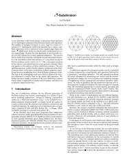
Figure 2: Example of a Laplacian eigenfunction f(x, y) =<br />
cos(πx) cos(πy). The corresponding Morse-Smale complex is depicted<br />
by black arrows.<br />
3.2 Square Patches<br />
Let f be an eigenfunction of the discrete Laplacian operator, i.e.,<br />
L f = −λ f. (4)<br />
The Laplacian operator is tightly related to discrete cosine transform<br />
[Strang 1999]. By intuition, we extend the relationship to<br />
locally developable surface: there exist two intrinsic parameter directions<br />
x <strong>and</strong> y such that f is a discrete analogon to a function of<br />
the form<br />
2006]). For each f[λ k ] we check the non-orthogonality measure<br />
(6) at all the extrema (in the simplified MSC). This will produce<br />
orthogonal c<strong>and</strong>idates to select from. Figure 3 shows an example<br />
of how this procedure allows us to find out the most orthogonal<br />
MSC.<br />
To evaluate Esquare, we consider the Hessian of (5)<br />
( )<br />
−α 2 cc αβ ss<br />
H[f(x, y)] = A<br />
αβ ss −β 2 cc<br />
where we set cc = cos(α x + φ x) cos(β y + φ y) <strong>and</strong> ss =<br />
sin(α x + φ x) sin(β y + φ y). At an extremum, we have cc = ±1<br />
<strong>and</strong> ss = 0. Hence<br />
H[f(<br />
πi − φx<br />
,<br />
α<br />
(<br />
πj − φy ∓A α<br />
2<br />
)] =<br />
β<br />
)<br />
0<br />
0 ∓A β 2 .<br />
This means that Esquare can be expressed by the ratio of the eigenvalues<br />
of the Hessian <strong>and</strong> hence it does not depend on the amplitude<br />
A (which may vary at different extrema).<br />
Since for a given eigenfunction f we cannot easily derive the intrinsic<br />
directions x <strong>and</strong> y, it is quite difficult to exploit (5) directly.<br />
However, we can replace f(x, y) by the local quadratic fit q(u, v)<br />
whose Hessian<br />
( )<br />
cuu c<br />
H[q(u, v)] =<br />
uv<br />
c uv c vv<br />
has approximately the same eigenvalues as H[f(x, y)]. This is obvious<br />
because the rotation between the (u, v) <strong>and</strong> the (x, y) coordinate<br />
systems only affect the eigenvectors, not the eigenvalues.<br />
From<br />
trace H[q(u, v)] = c uu + c vv ≈ −A (α 2 + β 2 )<br />
det H[q(u, v)] = c uu c vv − c 2 uv ≈ A 2 α 2 β 2<br />
at the extrema we conclude that<br />
Esquare = α4 + 2α 2 β 2 + β 4<br />
α 2 β 2 − 2 ≈<br />
(cuu + cvv)2<br />
− 2.<br />
c uu c vv − c 2 uv<br />
(7)<br />
f(x, y) = A cos(α x + φ x) cos(β y + φ y) (5)<br />
where α, β define the frequencies in x <strong>and</strong> y directions respectively,<br />
A is the amplitude, (φ x, φ y) defines the phase shift, <strong>and</strong> the eigenvalue<br />
is λ = α 2 + β 2 . The corresponding MSC is an affine grid<br />
consisting of two sets of lines with a slope of (β, α) <strong>and</strong> (−β, α)<br />
respectively. This affine grid turns out to be an orthogonal one if<br />
<strong>and</strong> only if α = β. See Figure 2 for a depiction of this situation.<br />
We use the “Multiresolution Spectral Analysis” technique [Dong<br />
et al. 2006] to solve the generalized eigenproblem on a large mesh,<br />
<strong>and</strong> then pick the eigenfunction for producing the best results. To<br />
find an eigenvalue λ whose eigenfunction f yields an as orthogonal<br />
as possible MSC, let<br />
Esquare = α2<br />
β 2 + β2<br />
α 2 = α4 + β 4<br />
α 2 β 2 (6)<br />
be a measure for the “non-orthogonality” of the MSC grid. Then<br />
we compute a small number of eigenfunctions f[λ k ] for several<br />
eigenvalues λ k around the estimated λ which is selected according<br />
to the number of critical points in the complex (c.f. [Dong et al.<br />
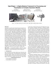
index = 22 32 35<br />
Esquare = 10.75 6.58 2.670<br />
Figure 3: Finding eigenfunctions with approximately orthogonal<br />
MSC. By testing eigenfunctions f[λ k ] for eigenvalues λ k around<br />
the estimated λ (center column), we can find the most orthogonal<br />
eigenfunction (right column) among them.<br />
3.3 Adaptive Size Control<br />
In order to preserve fine details in some surface regions without<br />
introducing redundant over-tesselation in other regions, we would
like to vary the distance between stationary points locally in a controlled<br />
fashion. Therefore, we exploit the physical meaning of the<br />
Laplace eigenproblem.<br />
The generalized eigenproblem in (3) can be viewed as a vibration<br />
analysis on the elastic membrane given by the input mesh. As discussed<br />
in [Vallet <strong>and</strong> Lévy 2007], we can interpret the Laplacian<br />
matrix L as a stiffness matrix, <strong>and</strong> D as a lumped mass matrix. The<br />
eigenvalue λ is related to the vibration frequency by ω = √ λ <strong>and</strong><br />
the eigenfunction f represents the corresponding stationary wave.<br />
From the theory of wave propagation in an elastic body [Alford<br />
et al. 1974], we have the following relationship:<br />
√<br />
stiffness<br />
wave speed = frequency × wavelength = k 1<br />
mass density<br />
<strong>and</strong> for the distance l between two adjacent extrema we obtain<br />
where k 1, k 2 are constant coefficients.<br />
l = k 2<br />
1<br />
√<br />
λD<br />
(8)<br />
Due to the surface area weights D i in (3), the underlying elastic<br />
body is assumed to have uniform material properties. Hence, the<br />
wave speed is nearly constant over the mesh <strong>and</strong> thus for a given<br />
eigenvalue (frequency), the stationary points of the eigenfunction<br />
are uniformly distributed. From (8), we can also underst<strong>and</strong> why<br />
the stationary points move closer to each other when the eigenvalue<br />
(frequency) is increasing.<br />
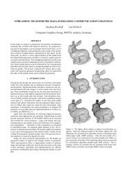
(a) (b) (c) (d)<br />
Figure 4: Creating a quadrangulation with adaptive density by<br />
changing the surface area weights D. (a) Local surface areas are<br />
scaled by 1, 3, <strong>and</strong> 6 in the gray, green, <strong>and</strong> red regions respectively.<br />
(b) The quasi-dual Morse-Smale complex constructed from<br />
the generalized eigenproblem. (c)(d) The front <strong>and</strong> back view of<br />
the quadrangulation result with smaller quads in the green <strong>and</strong> red<br />
regions.<br />
To control the cell size of the MSC, i.e., the density distribution of<br />
the eigenfunction’s stationary points, we can simply scale the corresponding<br />
entries in the lumped mass matrix D up (to increase the<br />
density) or down (to decrease it). Thus we can effectively adapt the<br />
resulting quadrilateral mesh density for better feature preserving.<br />
See Figure 4 for an example.<br />
In [Dong et al. 2006], the eigenproblem is solved without considering<br />
the mass matrix D <strong>and</strong> consequently the distance between<br />
stationary nodes in the MSC strongly depends on the tesselation of<br />
the input mesh. Our adaptive size control also provides a physical<br />
interpretation of the partial shifting technique used in [Dong et al.<br />
2006] which reduces the diagonal entries of the Laplacian matrix<br />
for some vertices. From the relation:<br />
(L − S)f = λf ⇔ Lf = λ(I + S)f<br />
with S being a diagonal matrix, we find that partial shifting actually<br />
corresponds to adding offsets to the corresponding entries of the<br />
mass matrix (while we apply a scaling factor). In the region with<br />
partial shifting, the wavelength becomes much shorter, so extrema<br />
more likely appear.<br />
3.4 Orientation Control<br />
In section 3.2 we already exploited the Hessian (of the continuous<br />
analogon) of the eigenfunction f to identify the function which<br />
leads to a MSC with an orthogonal structure. Here we take this idea<br />
even further by using the coefficients of the Hessian for orientation<br />
control.<br />
For eigenfunctions f with orthogonal MSC, we can assume the directional<br />
frequencies α <strong>and</strong> β to be equal <strong>and</strong> hence the Hessian of<br />
the continuous analogon (5) simplifies to<br />
( )<br />
H[f(x, y)] = Aα 2 −cc ss<br />
. (9)<br />
ss −cc<br />
( ( )<br />
1 −1<br />
The eigenvectors e + = <strong>and</strong> e<br />
1)<br />
− = of this matrix,<br />
i.e., the principal directions of f do not change with (x, y).<br />
1<br />
They coincide with the two orthogonal directions of the corresponding<br />
MSC.<br />
The basic idea of orientating the MSC is to take an eigenfunction f<br />
which has an approximately orthogonal MSC <strong>and</strong> to “twist” it towards<br />
a function with the property that the principal directions (i.e.,<br />
the eigenvectors of the Hessian) coincide with the prescribed direction<br />
field. Our approach is to add an energy term to the Laplace<br />
eigenproblem which penalizes the deviation of the principal directions.<br />
Again, instead of using the Hessian of (5) directly we use the Hessian<br />
of the local quadratic fit q(u, v). Since we have oriented the<br />
(u, v)-coordinate system such that its u-direction coincides with<br />
the prescribed direction field d i, we simply have to make sure that<br />
the principal directions of q(u, v) coincide with the main axes in<br />
(u, v)-parameter space. This is guaranteed if the Hessian of q(u, v)<br />
is a diagonal matrix. Hence, our local penalizing energy is<br />
(c i uv) 2 = < Q i uv, f > 2 .<br />
The total penalizing energy is then obtained by integration over the<br />
entire mesh, i.e.,<br />
E orient = ∑<br />
D i < Q i uv, f > 2 = ‖Q orient f‖ 2 . (10)<br />
v i ∈V<br />
As mentioned in [Dong et al. 2006], the angle between the edge<br />
direction of quasi-dual <strong>and</strong> primal complex is π/4, we can use the<br />
π/4 rotated direction field to make the orientation of a quasi-dual<br />
complex coincide with this direction field. See Figure 5 for orientation<br />
examples.<br />
3.5 Alignment Control<br />
When the input mesh has sharp or non-sharp feature lines, they<br />
should be represented by a sequence of polygon edges in the output.
(a) (b) (c)<br />
Figure 5: Orientation control on the torus model. (a) make the<br />
edges of the quasi-dual Morse-Smale complex coincide with the<br />
principal curvatures (b) rotate the direction field in (a) by 20 degree.<br />
(c) rotate the direction field in (a) by 45 degree.<br />
(a) (b) (c)<br />
Figure 6: Using alignment control to snap some edges of the quasidual<br />
MSC in (b) to the specified feature lines in (a). (c) shows the<br />
quasi-dual MSC for the unconstrained eigenproblem.<br />
Hence, besides orientation control we have to introduce control on<br />
feature alignment. Many feature detection techniques have been<br />
proposed, for example [Yoshizawa et al. 2005]. In this paper we<br />
assume that the relevant feature lines on the input mesh are given.<br />
In the local DCT approximation (5) of the eigenfunction f, we can<br />
observe that the edges of the primal MSC lie on the diagonals:<br />
(αx + φ x) ± (βy + φ y) = kπ, <strong>and</strong> the edges of dual MSC are<br />
on: αx + φ x = kπ <strong>and</strong> βy + φ y = kπ. These lines represent<br />
the set of symmetry axes of f. Hence in order to make the MSC of<br />
the function f align to a certain feature line l, we enforce f to be<br />
symmetric with respect to l.<br />
Let (û, ˆv) be a local parametrization such that the û-axis is aligned<br />
to the feature line l. Then the symmetry condition on f written in<br />
terms of the local quadratic approximation q(û, ˆv) is<br />
which is equivalent to<br />
q(û, −ˆv) = q(û, ˆv)<br />
cûˆv = 0 <strong>and</strong> cˆv = 0.<br />
Thus, the penalizing energy for feature alignment over the whole<br />
mesh becomes:<br />
E align = ∑ v i ∈l<br />
D i(< Q i ûˆv, f > 2 + < Q iˆv, f > 2 ) = ‖Q align f‖ 2 .<br />
(11)<br />
In the primal MSC case, we can expect that the feature is oriented<br />
along the prescribed tangent direction field d. In this case the<br />
parametrization (û, ˆv) coincides with (u, v) <strong>and</strong> the first condition<br />
cûˆv = 0 simply repeats the orientation condition. Consequently the<br />
penalizing energy for misalignment to the feature line l is simplified<br />
as<br />
E align = ∑ D i < Q i v, f > 2 . (12)<br />
v i ∈l<br />
3.6 Meshes with Boundaries<br />
The original framework proposed in [Dong et al. 2006] cannot h<strong>and</strong>le<br />
meshes with boundaries which are very common in practice.<br />
By treating boundaries of the mesh as feature lines, we can easily<br />
exploit the orientation <strong>and</strong> alignment control to h<strong>and</strong>le them.<br />
As shown in Figure 7 <strong>and</strong> Figure 8, we create a direction field which<br />
is perpendicular or parallel to the boundaries in the nearby region,<br />
<strong>and</strong> use the orientation control to ensure that some of the edges of<br />
the MSC are parallel with the boundaries. The alignment control<br />
finally snaps edges precisely to the boundaries. In Figure 8, we<br />
also add size controls to make the wavelength compatible with the<br />
alignment configuration (which will be discussed in section 5).<br />
(a) (b) (c) (d)<br />
Figure 7: H<strong>and</strong>le meshes with boundaries by treating boundaries<br />
as feature lines. (a) the direction field which is perpendicular to<br />
the boundaries (b) the unconstrained MSC which is not aligned<br />
with the boundaries. (c) some edges of the MSC are aligned with<br />
the boundaries by orientation <strong>and</strong> alignment control. (d) the final<br />
quadrangulation result.<br />
Since there is no appropriate definition of the Laplacian operator<br />
on boundaries, we use the definition proposed in [Vallet <strong>and</strong> Lévy<br />
2008]: if the edge [i, j] is on the border, the term of cot(β ij) in<br />
ω ij vanishes. This definition matches the FEM formulation with<br />
Neumann boundary conditions.<br />
3.7 Constrained Eigenproblem<br />
To eventually find a scalar function f on M which satisfies all the<br />
requirements, we first select a proper λ <strong>and</strong> D with the methods<br />
presented in Sections (3.2) <strong>and</strong> (3.3), then combine Equations (3),<br />
(10) <strong>and</strong> (11) to obtain:<br />
min<br />
f<br />
( ∥∥∥( √<br />
D<br />
−1<br />
L<br />
√<br />
D<br />
−1<br />
+ λI)<br />
√<br />
Df<br />
∥ ∥∥<br />
2<br />
+w 1‖Q orient f‖ 2 + w 2‖Q align f‖ 2)<br />
s.t.‖ √ Df‖ 2 = 1<br />
(a) (b) (c)<br />
(13)<br />
Figure 8: Quadrangulation on the car model. (a) the direction<br />
field. Different weights D are indicated by different color. (b) the<br />
quasi-dual Morse-Smale complex, (c) the final quadrilateral mesh.
where w 1 <strong>and</strong> w 2 are the user specified weights to balance the orientation<br />
energy, alignment energy <strong>and</strong> the quality of MSC (see Figure<br />
9). We experimentally find that w 1 = 0.5 <strong>and</strong> w 2 = 1.0 works<br />
well in all our results.<br />
The above constrained optimization problem are iteratively solved<br />
by the following equation:<br />
( ) ( ) (<br />
A J<br />
T<br />
k fk+1 0<br />
=<br />
(14)<br />
J k 0 ν 1)<br />
where ν is the Lagrange multiplier, <strong>and</strong><br />
A = ̂L T ̂L + w1Q T orient Q orient + w2QT align Q align<br />
̂L = ( √ D −1 L √ D −1 + λI) √ D<br />
J k = f T k D.<br />
In (14) we take f k to calculate the approximate Hessian matrix at<br />
iteration k + 1. By exploiting the block structure in (14), it can<br />
be solved efficiently through the following two equations with prefactorized<br />
the matrix A:<br />
(J k A −1 J T k )ν = −1<br />
Af k+1 = −νJ T k .<br />
(15)<br />
The iteration stops when the ‖ √ D(f k+1 − f k )‖ < 10 −7 . In our<br />
experiments, about 20 iterations are enough.<br />
the steepest ascending/descending lines starting from each saddle<br />
to a maximum/minimum, <strong>and</strong> use them to partition the mesh into<br />
quadrangular regions. We also use the cancellations [Edelsbrunner<br />
et al. 2003; timo Bremer et al. 2004] which eliminates<br />
a connected saddle-extremum pair each time to simplify the<br />
MSC. The priority of cancellation is ranked by their persistence<br />
[Edelsbrunner et al. 2002]. In practice, we only perform the<br />
anti − cancellation for the very high valency (larger than 7) extremum<br />
of MSC, <strong>and</strong> split it along the longest edge. This procedure<br />
is actually rarely used, because high valency extrema rarely occur<br />
in our experiments. If the quasi-dual MSC is required, we connect<br />
the maximum-minimum diagonal within each quadrangular region<br />
on the simplified primal MSC.<br />
The parameterization method proposed in [Dong et al. 2006] will<br />
relocate the edges of the MSC when swapping vertices across<br />
boundaries to adjust patches. As a result, after the iterative relaxation<br />
procedure, the parameterization often distorts the edge away<br />
from the feature lines. To accurately align the feature lines, we<br />
augment the original algorithm by edge constraints. The parameterization<br />
coordinates of vertices on the feature lines are interpolated<br />
from the corresponding nodes of the complex. Then we put<br />
these known values as hard constraints into the parameterization<br />
equations.<br />
The analysis of the performance, some additional results <strong>and</strong> the<br />
quality of the final quadrilateral meshes will be demonstrated in the<br />
following.<br />
|M| |M q| MSC Parameterization<br />
Car 2818 3360 0.65s 2.28s<br />
Rockarm 9405 9301 2.32s 19.08s<br />
Elephant 18074 18173 4.57s 51.19s<br />
Pegaso 23930 16693 5.84s 83.57s<br />
Table 1: Performance of our system.<br />
w 1 0.0 0.015 0.040 0.060 0.10 0.7<br />
max 3.70 1.82 1.98 2.30 2.46 1.14<br />
mean 3.32 1.502 0.98 0.84 0.67 0.23<br />
Figure 9: Visualization of how the eigenfunction f <strong>and</strong> the MSC<br />
change as more <strong>and</strong> more weight w 1 is put on the orientation. The<br />
other two rows show the maximum <strong>and</strong> average value of c 2 uv.<br />
After removing the topological noise using the algorithm proposed<br />
in [Dong et al. 2006] which includes cancellation(removing redundant<br />
saddle-extremum pairs) <strong>and</strong> anti-cancellation(the inverse of<br />
cancellation), we have constructed a quadrangular base complex<br />
over the mesh which satisfies all the input requirements. Then we<br />
build a parameterization over this complex <strong>and</strong> generate a regular<br />
d × d grid of quadrilaterals in this parametric domain with a userspecified<br />
density d.<br />
4 Implementation Details <strong>and</strong> Results<br />
Alike [Dong et al. 2006], we construct the MSC by<br />
the algorithm proposed in [Edelsbrunner et al. 2003;<br />
timo Bremer et al. 2004]. After classifying the critical<br />
points(maximum/minimum/saddle) of f, we construct<br />
Tabel 1 summarizes the size of some models <strong>and</strong> the performance<br />
of our system on these models. |M| <strong>and</strong> |M q| are the number<br />
of vertices of the input triangle mesh <strong>and</strong> output quadrangulation<br />
mesh respectively. The column named as MSC shows the time (in<br />
seconds) for solving the constrained eigenproblem. And the column<br />
Parameterization lists the time used in the parameterization.<br />
Running times are measured on a 1.8G Intel DualCore 2 CPU with<br />
2GB memory. We solve all the sparse linear equations by UMF-<br />
PACK [Davis 2004].<br />
Our method is insensitive to the noise in the direction field, <strong>and</strong> can<br />
even apply to noisy geometry. In Figure 10, we directly use the direction<br />
field which comes from the curvature tensor <strong>and</strong> weight the<br />
orientation energy by the curvature tensor magnitude. Although the<br />
hair of the David head model is very noisy, the orientation control<br />
still works well. Even in the hair region, some singularities automatically<br />
appear to make the quadrangulation result consistent with<br />
some of the significant features in the direction field. Comparing<br />
with [Ray et al. 2006; Kälberer et al. 2007], it’s an advantage that<br />
our method can optimize irregular vertex positions for such noisy<br />
direction field.<br />
Finally, we measure the quality of our results. The number of irregular<br />
vertices, the distribution of the angle <strong>and</strong> edge length can be<br />
found in Figure 11. Both models are constrained by direction field,<br />
<strong>and</strong> size control is added on the face of pegaso horse to capture<br />
more details. By virtue of the period property of the eigenfunction,<br />
our result has only a few irregular vertices.
(a) (b) (c) (d) (e)<br />
Figure 11: Quadrangulation on the pegaso horse <strong>and</strong> elephant model. (a) the direction field. Different weights D are indicated by different<br />
color on the pegaso horse. (b) the quasi-dual Morse-Smale complex, (c)(d) the final quadrilateral mesh from the left <strong>and</strong> right view, (e) the<br />
plot of quality measurement.<br />
when the applied constraints conflict with the period property of<br />
the eigenfunction. As shown in Figure 12 , the F<strong>and</strong>isk model has<br />
many corners, <strong>and</strong> the distribution of them is very irregular. It’s a<br />
tough job to set proper size, orientation <strong>and</strong> alignment controls to<br />
get a scalar function which has stationary points on every corner.<br />
(a) (b) (c) (d)<br />
Figure 10: Our method can directly apply to noisy geometry. (a)<br />
the direction field which comes from the curvature tensor. (b) the<br />
quasi-dual Morse-Smale complex. (c)(d) the final quadrilateral<br />
mesh from two views.<br />
5 Discussion <strong>and</strong> Future Work<br />
In this paper, we have presented a method to control the topological<br />
structure of the quadrangulation result by finding the optimal<br />
Morse-Smale complex. The scalar function from which the MSC<br />
is derived is approximated locally by DCT basis function <strong>and</strong> a<br />
quadratic polynomial. We look into the relationships between the<br />
MSC <strong>and</strong> the DCT basis function, then using the quadratic polynomial<br />
to represent these relationships. By solving a constrained least<br />
square problem which is dominated by a generalized eigenproblem,<br />
we find the best scalar function according to the requirements.<br />
After getting a good topological structure derived from the scalar<br />
function, we parameterize it over the surface. For better feature<br />
preserving, edge constraints are introduced into the global smooth<br />
parameterization framework.<br />
Our method can generate the quadrangulation result with low distortion<br />
<strong>and</strong> only a few number of the irregular vertices. But in<br />
some cases, the result may not follow user’s intention, especially<br />
Figure 12: Using the size, orientation <strong>and</strong> alignment controls can<br />
get an approximately feature aligned result. But a perfect result<br />
requires more controls except for the ones proposed in this paper.<br />
The alignment control cannot work well on some complex feature<br />
line configurations. It is hard to simultaneously align the edges of<br />
MSC with all feature lines if the distance between them is contradict<br />
with wavelength, e.g. the distance between two parallel feature<br />
lines is quite different from the integer times of the wavelength/4.<br />
We also tried a constrain to ensure the corners to be nodes of the<br />
MSC (see Figure 13), which is similar to the alignment control but<br />
without the requirement of orientation control. The nodes of the<br />
MSC are saddles or extrema of f <strong>and</strong> hence at the positions where<br />
nodes appear, the following equation must hold:<br />
0 = ∂f(u,v)<br />
∂u<br />
= c u = < Q u, f ><br />
0 = ∂f(u,v)<br />
∂v<br />
= c v = < Q v, f > .<br />
(16)<br />
By including above linear equations as hard constraints into (13),<br />
we can impose node position constraints. However, applying po-
(a) (b) (c)<br />
Figure 13: We can make nodes lie on the corners of the gargoyle<br />
model by position control. (a) without node position control. (b)<br />
the node positions are spedified by the user on some vertices of the<br />
model (indicated by yellow spheres), (c) the Morse-Smale Complex<br />
with node position control.<br />
sition constraints at sparse locations on the mesh does not guarantee<br />
that the arcs of the MSC properly align to the feature lines in<br />
between <strong>and</strong> hence alignment control along feature lines remains<br />
necessary.<br />
It would be another interesting control to constrain both the position<br />
<strong>and</strong> valance of irregular vertex simultaneously. As pointed out in<br />
[Tong et al. 2006], the optimal quadrangulation should match the<br />
curvature tensor. The position <strong>and</strong> valance of a MSC node should<br />
reflect the local average of Gaussian curvature, which is heavily<br />
related to the Hessian of f(x, y) <strong>and</strong> q(u, v).<br />
6 Acknowledgments<br />
We would like to thank the reviewers for their valuable comments.<br />
This work is supported in partial by NSFC (No.60703039), the<br />
973 Program of China (No.2002CB312100), the Program for New<br />
Century Excellent Talents in University of China (No. NCET-06-<br />
0516), Fok Ying Tung Education Fund, UMIC Research Cluster<br />
<strong>and</strong> AICES Graduate School (both funded by DFG).<br />
References<br />
ALFORD, R. M., KELLY, K. R., AND BOORE, D. M. 1974. Accuracy<br />
of finite-difference modeling of the acoustic wave equation. Geophysics<br />
39, 6 (December), 834–842.<br />
ALLIEZ, P., COHEN-STEINER, D., DEVILLERS, O., LÉVY, B., AND DES-<br />
BRUN, M. 2003. Anisotropic polygonal remeshing. ACM Trans. Graph.<br />
22, 3, 485–493.<br />
ALLIEZ, P., UCELLI, G., GOTSMAN, C., AND ATTENE, M. 2005. Recent<br />
advances in remeshing of surfaces.<br />
BOIER-MARTIN, I., RUSHMEIER, H., AND JIN, J. 2004. Parameterization<br />
of triangle meshes over quadrilateral domains. In SGP ’04: Proceedings<br />
of the 2004 Eurographics/ACM SIGGRAPH symposium on Geometry<br />
processing, ACM, 193–203.<br />
BOTSCH, M., AND PAULY, M. 2007. Course 23: Geometric modeling<br />
based on polygonal meshes. In SIGGRAPH courses.<br />
DAVIS, T. A. 2004. A column pre-ordering strategy for the unsymmetricpattern<br />
multifrontal method. ACM Trans. Math. Softw. 30, 2, 165–195.<br />
DONG, S., KIRCHER, S., AND GARLAND, M. 2005. Harmonic functions<br />
for quadrilateral remeshing of arbitrary manifolds. Comput. Aided Geom.<br />
Des. 22, 5, 392–423.<br />
DONG, S., BREMER, P.-T., GARLAND, M., PASCUCCI, V., AND HART,<br />
J. C. 2006. Spectral surface quadrangulation. ACM Trans. Graph. 25,<br />
3, 1057–1066.<br />
EDELSBRUNNER, H., LETSCHER, D., AND ZOMORODIAN, A. 2002.<br />
Topological persistence <strong>and</strong> simplification. Discrete <strong>Computer</strong> Geometry<br />
28, 511–533.<br />
EDELSBRUNNER, H., HARER, J., AND ZOMORODIAN, A. 2003. Hierarchical<br />
morse-smale complexes for piecewise linear 2-manifolds. Discrete<br />
<strong>and</strong> Computational Geometry 30, 1, 87–107.<br />
FISHER, M., SCHRÖDER, P., DESBRUN, M., AND HOPPE, H. 2007. Design<br />
of tangent vector fields. In SIGGRAPH ’07: ACM SIGGRAPH 2007<br />
papers, ACM, 56.<br />
GU, X., AND YAU, S.-T. 2003. Global conformal surface parameterization.<br />
In SGP ’03: Proceedings of the 2003 Eurographics/ACM SIG-<br />
GRAPH symposium on Geometry processing, Eurographics Association,<br />
127–137.<br />
IGARASHI, T., MOSCOVICH, T., AND HUGHES, J. F. 2005. As-rigid-aspossible<br />
shape manipulation. ACM Trans. Graph. 24, 3, 1134–1141.<br />
KÄLBERER, F., NIESER, M., , AND POLTHIER, K. 2007. Quadcover -<br />
surface parameterization using branched coverings. <strong>Computer</strong> <strong>Graphics</strong><br />
Forum 26, 3 (September), 375–384.<br />
KHODAKOVSKY, A., LITKE, N., AND SCHRÖDER, P. 2003. Globally<br />
smooth parameterizations with low distortion. In SIGGRAPH ’03: ACM<br />
SIGGRAPH 2003 <strong>Paper</strong>s, ACM, 350–357.<br />
LI, W.-C., RAY, N., AND LÉVY, B. 2006. Automatic <strong>and</strong> interactive mesh<br />
to t-spline conversion. In SGP ’06: Proceedings of the fourth Eurographics<br />
symposium on Geometry processing, Eurographics Association, 191–<br />
200.<br />
MARINOV, M., AND KOBBELT, L. 2004. Direct anisotropic quad-dominant<br />
remeshing. In PG ’04: Proceedings of the <strong>Computer</strong> <strong>Graphics</strong> <strong>and</strong> Applications,<br />
12th Pacific Conference on (PG’04), IEEE <strong>Computer</strong> Society,<br />
207–216.<br />
MARINOV, M., AND KOBBELT, L. 2006. A robust two-step procedure<br />
for quad-dominant remeshing. <strong>Computer</strong> <strong>Graphics</strong> Forum 25, 3 (Sept.),<br />
537–546.<br />
MEYER, M., DESBRUN, M., SCHRÖDER, P., AND BARR, A. H. Discrete<br />
differential-geometry operators for triangulated 2-manifolds.<br />
PINKALL, U., AND POLTHIER, K. 1993. Computing discrete minimal<br />
surfaces <strong>and</strong> their conjugates. Experimental Mathematics 2, 1, 15–36.<br />
RAY, N., LI, W. C., LÉVY, B., SHEFFER, A., AND ALLIEZ, P. 2006.<br />
Periodic global parameterization. ACM Trans. Graph. 25, 4, 1460–1485.<br />
SHI, L., AND YU, Y. 2004. Inviscid <strong>and</strong> incompressible fluid simulation<br />
on triangle meshes: Research articles. Comput. Animat. Virtual Worlds<br />
15, 3-4, 173–181.<br />
STRANG, G. 1999. The discrete cosine transform. SIAM Review 41, 1,<br />
135–147.<br />
TIMO BREMER, P., EDELSBRUNNER, H., HAMANN, B., AND PASCUCCI,<br />
V. 2004. A topological hierarchy for functions on triangulated surfaces.<br />
IEEE Transactions on Visualization <strong>and</strong> <strong>Computer</strong> <strong>Graphics</strong> 10, 385–<br />
396.<br />
TONG, Y., ALLIEZ, P., COHEN-STEINER, D., AND DESBRUN, M. 2006.<br />
Designing quadrangulations with discrete harmonic forms. In SGP ’06:<br />
Proceedings of the fourth Eurographics symposium on Geometry processing,<br />
Eurographics Association, 201–210.<br />
VALLET, B., AND LÉVY, B. 2007. Spectral geometry processing with<br />
manifold harmonics. Technical Report (April).<br />
VALLET, B., AND LÉVY, B. 2008. Spectral geometry processing with<br />
manifold harmonics. <strong>Computer</strong> <strong>Graphics</strong> Forum 27, 2 (Apr.), 251–260.<br />
YOSHIZAWA, S., BELYAEV, A., AND SEIDEL, H.-P. 2005. Fast <strong>and</strong> robust<br />
detection of crest lines on meshes. In SPM ’05: Proceedings of the 2005<br />
ACM symposium on Solid <strong>and</strong> physical modeling, ACM, 227–232.