Lap Time Optimization of a Sports Series Hybrid Electric Vehicle
Lap Time Optimization of a Sports Series Hybrid Electric Vehicle
Lap Time Optimization of a Sports Series Hybrid Electric Vehicle

You also want an ePaper? Increase the reach of your titles
YUMPU automatically turns print PDFs into web optimized ePapers that Google loves.
Proceedings <strong>of</strong> the World Congress on Engineering 2013 Vol III,<br />
WCE 2013, July 3 - 5, 2013, London, U.K.<br />
<strong>Lap</strong> <strong>Time</strong> <strong>Optimization</strong> <strong>of</strong><br />
a <strong>Sports</strong> <strong>Series</strong> <strong>Hybrid</strong> <strong>Electric</strong> <strong>Vehicle</strong><br />
Roberto Lot and Simos A. Evangelou<br />
Abstract—This paper illustrates a methodology for the lap<br />
time optimization <strong>of</strong> a race series hybrid electric vehicle based<br />
on the indirect optimal control approach. More specifically, for<br />
a vehicle with given characteristics running on a given track, the<br />
optimal trajectory and powertrain power flow that minimize the<br />
lap time are found. The paper presents a parametric model <strong>of</strong> a<br />
sports series hybrid electric vehicle, illustrates the optimization<br />
method and discusses simulation results.<br />
Index Terms—hybrid electric vehicle, vehicle dynamics, optimal<br />
control, lap time optimization.<br />
I. INTRODUCTION<br />
HYBRID electric vehicles (HEVs) are becoming more<br />
popular due to their potential to address climate change<br />
and the demand for a limited, but increasingly expensive,<br />
supply <strong>of</strong> fossil fuels. In addition, a new category <strong>of</strong> sports<br />
and race HEVs is emerging [1], [2]. Although the synergy<br />
between multiple energy sources in HEV powertrains is<br />
normally used to bring reductions in fuel consumption and<br />
noxious emissions, in racing the main interest is about<br />
performance and lap time minimization.<br />
In the case <strong>of</strong> road HEVs various control techniques have<br />
been proposed in the literature for the powertrain energy<br />
management, ranging from rule-based to optimisation-based<br />
[3]–[9]. This paper presents a global optimisation-based control<br />
approach that utilises indirect optimal control techniques<br />
to optimise not only the powertrain energy flow but also the<br />
trajectory <strong>of</strong> a racing HEV inside a given race circuit. The<br />
methodology is established by utilising symbolic dynamic<br />
vehicle modelling <strong>of</strong> appropriate complexity, together with<br />
computationally efficient optimal control s<strong>of</strong>tware [10].<br />
II. MATHEMATICAL MODEL<br />
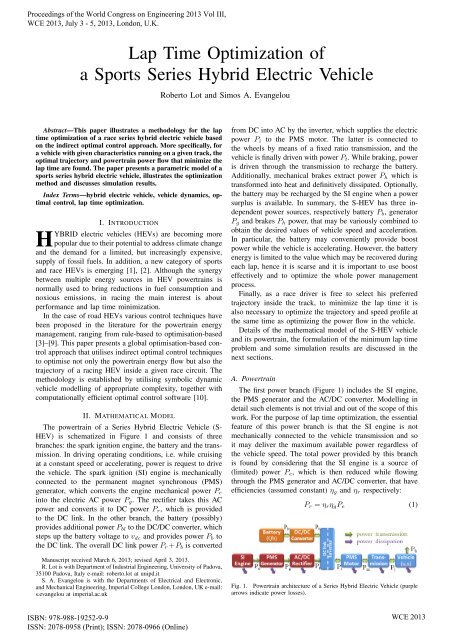
The powertrain <strong>of</strong> a <strong>Series</strong> <strong>Hybrid</strong> <strong>Electric</strong> <strong>Vehicle</strong> (S-<br />
HEV) is schematized in Figure 1 and consists <strong>of</strong> three<br />
branches: the spark ignition engine, the battery and the transmission.<br />
In driving operating conditions, i.e. while cruising<br />
at a constant speed or accelerating, power is request to drive<br />
the vehicle. The spark ignition (SI) engine is mechanically<br />
connected to the permanent magnet synchronous (PMS)<br />
generator, which converts the engine mechanical power P e<br />
into the electric AC power P g . The rectifier takes this AC<br />
power and converts it to DC power P r , which is provided<br />
to the DC link. In the other branch, the battery (possibly)<br />
provides additional power P bl to the DC/DC converter, which<br />
steps up the battery voltage to v dc and provides power P b to<br />
the DC link. The overall DC link power P r +P b is converted<br />
Manuscript received March 6, 2013; revised April 3, 2013.<br />
R. Lot is with Department <strong>of</strong> Industrial Engineering, University <strong>of</strong> Padova,<br />
35100 Padova, Italy e-mail: roberto.lot at unipd.it<br />
S. A. Evangelou is with the Departments <strong>of</strong> <strong>Electric</strong>al and Electronic,<br />
and Mechanical Engineering, Imperial College London, London, UK e-mail:<br />
s.evangelou at imperial.ac.uk<br />
from DC into AC by the inverter, which supplies the electric<br />
power P i to the PMS motor. The latter is connected to<br />
the wheels by means <strong>of</strong> a fixed ratio transmission, and the<br />
vehicle is finally driven with power P t . While braking, power<br />
is driven through the transmission to recharge the battery.<br />
Additionally, mechanical brakes extract power P h which is<br />
transformed into heat and definitively dissipated. Optionally,<br />
the battery may be recharged by the SI engine when a power<br />
surplus is available. In summary, the S-HEV has three independent<br />
power sources, respectively battery P b , generator<br />
P g and brakes P h power, that may be variously combined to<br />
obtain the desired values <strong>of</strong> vehicle speed and acceleration.<br />
In particular, the battery may conveniently provide boost<br />
power while the vehicle is accelerating. However, the battery<br />
energy is limited to the value which may be recovered during<br />
each lap, hence it is scarse and it is important to use boost<br />
effectively and to optimize the whole power management<br />
process.<br />
Finally, as a race driver is free to select his preferred<br />
trajectory inside the track, to minimize the lap time it is<br />
also necessary to optimize the trajectory and speed pr<strong>of</strong>ile at<br />
the same time as optimizing the power flow in the vehicle.<br />
Details <strong>of</strong> the mathematical model <strong>of</strong> the S-HEV vehicle<br />
and its powertrain, the formulation <strong>of</strong> the minimum lap time<br />
problem and some simulation results are discussed in the<br />
next sections.<br />
A. Powertrain<br />
The first power branch (Figure 1) includes the SI engine,<br />
the PMS generator and the AC/DC converter. Modelling in<br />
detail such elements is not trivial and out <strong>of</strong> the scope <strong>of</strong> this<br />
work. For the purpose <strong>of</strong> lap time optimization, the essential<br />
feature <strong>of</strong> this power branch is that the SI engine is not<br />
mechanically connected to the vehicle transmission and so<br />
it may deliver the maximum available power regardless <strong>of</strong><br />
the vehicle speed. The total power provided by this branch<br />
is found by considering that the SI engine is a source <strong>of</strong><br />
(limited) power P e , which is then reduced while flowing<br />
through the PMS generator and AC/DC converter, that have<br />
efficiencies (assumed constant) η g and η r respectively:<br />
P r = η r η g P e (1)<br />
Fig. 1. Powertrain architecture <strong>of</strong> a <strong>Series</strong> <strong>Hybrid</strong> <strong>Electric</strong> <strong>Vehicle</strong> (purple<br />
arrows indicate power losses).<br />
ISBN: 978-988-19252-9-9<br />
ISSN: 2078-0958 (Print); ISSN: 2078-0966 (Online)<br />
WCE 2013
Proceedings <strong>of</strong> the World Congress on Engineering 2013 Vol III,<br />
WCE 2013, July 3 - 5, 2013, London, U.K.<br />
The second power branch includes the battery and the<br />
DC/DC converter that steps up the low voltage on the battery<br />
side to a high voltage on the DC link side. The battery state<br />
<strong>of</strong> charge is described by the following differential equation:<br />
d<br />
dt Q b = −i b (2)<br />
where Q b is the actual charge and i b the current <strong>of</strong> the battery,<br />
assumed positive during the discharge phase. Moreover, the<br />
battery power (on the low voltage side) is:<br />
P bl = i b v b (3)<br />
where v b is the closed circuit voltage <strong>of</strong> the battery, which<br />
depends both on the battery charge Q b and current i b . Such<br />
dependence may be expressed in terms <strong>of</strong> the electrochemical<br />
parameters and an equivalent electrical circuit [11], [12] as<br />
follows:<br />
v b = E b −Ri b = E 0 +<br />
(<br />
1 − Q )<br />
max<br />
+Ae B(Q−Qmax) −Ri b<br />
Q<br />
(4)<br />
where E b is the open circuit voltage, R b is the internal<br />
resistance, E 0 is the nominal voltage, Q max is the capacity<br />
<strong>of</strong> the battery, and A, B are two additional constants. The<br />
DC/DC converter is simply modelled as a static element<br />
having a constant efficiency η dc . Since the converter is bidirectional,<br />
the power conversion may be described by means<br />
<strong>of</strong> the following equation:<br />
P b = η sign(P b)<br />
dc<br />
P bl (5)<br />
where P b is the battery power on the DC link side. The<br />
efficiency is adjusted according to the direction <strong>of</strong> the power<br />
flow, i.e. when the positive power flows from the battery to<br />
the DC link P b = η dc P bl , on the contrary when the negative<br />
power flows from the DC link to charge the battery P bl =<br />
η dc P b .<br />
Power flow is then collected by the DC link, which drives<br />
a bidirectional inverter. Similarly to the rectifier, the inverter<br />
is simply modelled by means <strong>of</strong> a constant efficiency factor<br />
η i , therefore the power balance <strong>of</strong> the DC link and inverter<br />
is described by the following equation:<br />
P i = η sign(Pr+P bl)<br />
i (P r + P bl ) (6)<br />
where once again the efficiency is adjusted according to the<br />
direction <strong>of</strong> the power flow sign(P r + P bl ). The inverter<br />
supplies the electric motor/generator, which is a 3-phase<br />
star-connected PMS machine. PMS machines combine a<br />
number <strong>of</strong> attractive features when used in hybrid vehicle<br />
applications, such as higher torque-to-inertia ratio and power<br />
density than ones <strong>of</strong> induction or wound-rotor synchronous<br />
machines. The dynamic electro-magnetic behaviour <strong>of</strong> the<br />
PMS machine may be effectively described in the rotor d−q<br />
reference frame [13] by the following non-linear differential<br />
equations:<br />
d<br />
L q<br />
dt i d = v d − Ri d + pωLi q (7a)<br />
d<br />
L q<br />
dt i q = v q − Ri q − pωLi q + λ (7b)<br />
where i d , v d and i q , v q are the direct and quadrature components<br />
<strong>of</strong> armature currents and terminal voltages, ω is the<br />
rotor angular speed, while the other parameters are described<br />
in Table I. Equations (7) model only the power losses due<br />
the resistance R <strong>of</strong> the stator copper windings, while in<br />
reality there are other electromagnetic dissipation sources<br />
[14] such as Eddy current losses (∝ ω 2 ) and hysteresis losses<br />
(∝ ω 2 ), while mechanical losses [14] include bearing losses<br />
(∝ ω) and windage losses (∝ ω 5 ). These additional losses<br />
are modelled in the dynamic equation <strong>of</strong> the rotor as follows:<br />
J d dt ω = 3 2 pλi q + T l + T d (ω) (8)<br />
where J is the rotor inertia, T l is the mechanical torque<br />
exchanged with the trasmission, and T d (ω) is the dissipation<br />
torque. The control strategy <strong>of</strong> the machine [15] uses a null<br />
direct current i d = 0. To further simplify the model, it may<br />
be observed that the dynamics <strong>of</strong> electromagnetic phenomena<br />
are much faster than mechanical ones, hence transient currents<br />
may be neglected. The inertia torque J d dtω is neglected<br />
also, as the motor inertia is much smaller than the vehicle<br />
inertia to which it is rigidly connected. These assumptions<br />
lead to the simplification <strong>of</strong> differential equations (7), (8)<br />
into a set <strong>of</strong> steady-state algebraic equations, which may be<br />
easily solved in term <strong>of</strong> currents and voltages, leading to<br />
the following equation for the input power P i (exchanged<br />
with the inverter) and output power P m (exchanged with the<br />
transmission):<br />
P i = ω(T l + T d ) − 2 3 R (T l + T d ) 2<br />
P m = ωT l<br />
(pλ) 2<br />
(9a)<br />
(9b)<br />
Equations (9) are capable <strong>of</strong> describing the reversible PMS<br />
machine both when it works as a generator, i.e. with positive<br />
power, load torque and quadrature current, or when it<br />
works as a motor, i.e. with negative power, load torque and<br />
quadrature current. According to such conventions, the PMS<br />
efficiency is:<br />
( ) sign(Pi)<br />
Pm<br />
η m =<br />
(10)<br />
P i<br />
and it is reported in Figure 2. The PMS machine efficiency<br />
is very high in a wide range <strong>of</strong> operating condition, even if<br />
it is very poor at low speeds, where the resistance losses Ri 2 q<br />
are predominant, and at low torques, where the mechanical<br />
losses ωT d (ω) are predominant. The figure also shows the<br />
current i q , which is√<br />
roughly proportional to the torque, and<br />
the overall voltage vq 2 + vd 2 , which is roughly proportional<br />
to the speed. The PMS motor is connected to the transmission<br />
and finally to the wheels in a way that the velocity ratio<br />
between the motor angular speed ω and the vehicle forward<br />
speed v is constant:<br />
τ = ω (11)<br />
u<br />
It is assumed that the transmission has a constant efficiency<br />
η t , the bi-directional power flow is hence modelled with the<br />
following equation:<br />
P t = η sign(Pm)<br />
t P m (12)<br />
i.e. when positive power flows form the PMS motor to the<br />
vehicle P t = η t P m , on the contrary when negative power<br />
flows from the vehicle to the battery P m = η t P t .<br />
Brakes are simply modelled as power withdrawal, i.e a<br />
source <strong>of</strong> negative power P h , which is converted into heat<br />
and dissipated.<br />
ISBN: 978-988-19252-9-9<br />
ISSN: 2078-0958 (Print); ISSN: 2078-0966 (Online)<br />
WCE 2013
Proceedings <strong>of</strong> the World Congress on Engineering 2013 Vol III,<br />
WCE 2013, July 3 - 5, 2013, London, U.K.<br />
torque [N]<br />
200<br />
100<br />
−100<br />
−200<br />
−300<br />
0.9<br />
0.92<br />
0.8<br />
0.50.5<br />
0.8<br />
0.94<br />
0.85<br />
0 0.5<br />
0.85<br />
0.9<br />
−100<br />
0.92<br />
0.95<br />
200<br />
0.95<br />
0.94<br />
0.95<br />
400<br />
0.92<br />
0.94<br />
0.9<br />
0<br />
100<br />
200<br />
0.8<br />
0.85<br />
0.9<br />
0.92<br />
0.85<br />
−400<br />
0 1000 2000 3000 4000 5000<br />
speed [rpm]<br />
Fig. 2. PMS machine efficiency (solid black), current (horizontal dotted red)<br />
and voltage (vertical dotted blue). Positive torques correspond to generator,<br />
and negative torques correspond to motor operating conditions.<br />
By coupling and manipulating equations (5), (6), (9),<br />
(10), and (12), the vehicle power flow may be completely<br />
described as a function <strong>of</strong> three independent power sources,<br />
respectively the generator P g , battery P b , and brakes P h , as<br />
follows:<br />
P e = ηe −1 P g (13a)<br />
P r = η r P g<br />
(13b)<br />
P bl = η − sign P b<br />
dc<br />
P b (13c)<br />
P i = η sign(ηrPg+P b)<br />
i (η r P g + P b ) (13d)<br />
P t = (η i η m η t ) sign(ηrPg+P b) (η r P g + P b )<br />
0.8<br />
0.5<br />
600<br />
(13e)<br />
The only dynamic variable <strong>of</strong> the powertrain is the battery<br />
charge Q b , while any other variable may algebraically be<br />
expressed as a function <strong>of</strong> P g , P b , P h .<br />
B. <strong>Vehicle</strong> and track<br />
This section illustrates the model used to capture the<br />
vehicle gross motion on the track for the purpose <strong>of</strong> trajectory<br />
and speed pr<strong>of</strong>ile optimization. The vehicle is modelled as<br />
a single-track rigid body, running on a horizontal flat track<br />
(Figure 3). The equations <strong>of</strong> motion in the longitudinal and<br />
Fig. 3.<br />
Single-track vehicle model.<br />
lateral directions are respectively:<br />
( ) d<br />
m<br />
dt u − Ωv = S r + S f cos δ − F f sin δ − F D (14)<br />
( ) d<br />
m<br />
dt v + Ωu = F r + S f sin δ + F f cos δ (15)<br />
where m is the vehicle mass, u and v are respectively the<br />
longitudinal and lateral speed, Ω is the yaw rate, (S f , F f )<br />
and (S r , F r ) are the longitudinal and lateral forces respectively<br />
on the front and rear axle, F D = 1 2 ρC DAu 2 is the<br />
aerodynamic drag resistance, and δ is the steering angle. The<br />
equation for the yaw motion is:<br />
I G<br />
d<br />
dt Ω = aF f cos δ + S f sin δ − bF r (16)<br />
while I G is the yaw moment <strong>of</strong> inertia, while a and b are the<br />
distance from the vehicle center <strong>of</strong> gravity (CoG) respectively<br />
<strong>of</strong> the front and rear axle.<br />
Tire longitudinal forces are strictly related to the power<br />
flow (13), in particular the propulsive power is transferred<br />
to the real axle only, while braking power is distributed on<br />
both axle with constant ratio r b :<br />
S f = r b min(P t + P h , 0)<br />
(17a)<br />
u<br />
S r = P t + P h − r b min(P t + P h , 0)<br />
(17b)<br />
u<br />
where suffixes f and r refer to the front and rear axle.<br />
<strong>Vehicle</strong> directionality is controlled by means <strong>of</strong> the steering<br />
angle δ. Tire lateral forces are assumed to be proportional<br />
to the cornering stiffness K, (small) sideslip angle λ and tire<br />
vertical load N as follows:<br />
(<br />
F f = k f λ f ≃ K f δ − aΩ + v )<br />
N f (18a)<br />
u<br />
bΩ − v<br />
F r = k r λ r ≃ K r N r (18b)<br />
u<br />
Tire loads are calculated taking into account the load transfer<br />
from the front to the rear axle during traction (and vice versa<br />
during braking), according to the (approximate) expressions:<br />
N r =<br />
a<br />
a + b mg + h<br />
a + b (S r + S f ) (19a)<br />
N f =<br />
b<br />
a + b mg − h<br />
a + b (S r + S f ) (19b)<br />
where h is the vehicle center <strong>of</strong> gravity height. The track<br />
is assumed to be flat and to lay on the horizontal plane<br />
xy. The curvature Θ <strong>of</strong> the track reference line Γ may be<br />
calculated from its cartesian coordinates (x, y) as a function<br />
<strong>of</strong> the travelled space s as follows:<br />
√ (d2 ) 2 ( ) 2<br />
x d2 y<br />
Θ(s) =<br />
ds 2 +<br />
ds 2 (20)<br />
To add the second dimension <strong>of</strong> the strip-like track model it<br />
is sufficient to specify the distance from the borders, which<br />
possibly depends on the position s. To track the position<br />
and orientation <strong>of</strong> the vehicle, it is very convenient to use<br />
the triple <strong>of</strong> curvilinear coordinates (s, n, α), where s and n<br />
are respectively the longitudinal and lateral position on the<br />
road strip and α is the vehicle heading relative to the road.<br />
As depicted in Figure 3, such coordinates are related to the<br />
vehicle speeds by the following differential relations:<br />
d<br />
dt<br />
d<br />
dt<br />
d<br />
n = u sin α + v cos α<br />
dt (21b)<br />
s =<br />
u cos α − v sin α<br />
1 − n Θ(s)<br />
u cos α − v sin α<br />
α = Ω − Θ(s)<br />
1 − n Θ(s)<br />
(21a)<br />
(21c)<br />
In conclusion, sections II-A and II-B describe the power<br />
train flow and the vehicle gross motion as a function <strong>of</strong> 7<br />
variables x(t) = {Q b , u, v, Ω, s, n, α} T and 4 control inputs<br />
u(t) = {P g , P b , P h , δ} T .<br />
ISBN: 978-988-19252-9-9<br />
ISSN: 2078-0958 (Print); ISSN: 2078-0966 (Online)<br />
WCE 2013
Proceedings <strong>of</strong> the World Congress on Engineering 2013 Vol III,<br />
WCE 2013, July 3 - 5, 2013, London, U.K.<br />
TABLE I<br />
MODEL PARAMETERS<br />
Symbol Value Parameter<br />
m 1050 kg vehicle mass<br />
h 0.450 m center <strong>of</strong> gravity (CoG) height<br />
a 1.150 m CoG to front axle<br />
b 1.000 m CoG to rear axle distancee<br />
I z 800 kg m 2 yaw moment <strong>of</strong> inertia<br />
1<br />
2 ρC DA 0.378 kg/m aerodynamic drag factor<br />
K r, K f 20 rad −1 tires non-dimensional sideslip stiffness<br />
µ r, µ f 1.05 tires friction coefficient<br />
r b 0.60 braking torque ratio on the front axle<br />
P e,max 125 kW SI engine max power<br />
E 0 200 V battery nominal voltage<br />
Q max 10 Ah battery capacity<br />
i b,d 100 A battery max discharging current<br />
i b,c 50 A battery max recharging current<br />
R b 0.200 Ω Battery internal resistance<br />
v dc 1000 V DC link voltage<br />
p 6 number <strong>of</strong> pole pairs <strong>of</strong> the PMS motor<br />
R 0.040 Ω PMS stator resistance<br />
L d , L q 450 mH stator inductances <strong>of</strong> PMS motor<br />
λ 0.20 Wb rotor magnetic flux <strong>of</strong> PMS motor<br />
i m,max 250 A max current <strong>of</strong> PMS motor<br />
τ 9 transmission ratio<br />
η r 0.96 rectifier efficiency<br />
η dc 0.96 DC/DC converter efficiency<br />
η i 0.96 inverter efficiency<br />
η t 0.85 transmission efficiency (tires included)<br />
III. THE MINIMUM LAP TIME PROBLEM<br />
The minimum lap time problem consists in finding the<br />
vehicle control inputs that minimize the time T necessary to<br />
move the vehicle from the starting line to the finish one <strong>of</strong> the<br />
given track, by satisfying the mechanical equations <strong>of</strong> motion<br />
as well as inequality constraints such as tires adherence, max<br />
power, track width, etc. As the final value T <strong>of</strong> the time<br />
variable t is clearly undefined, while the curvilinear abscissa<br />
s varies from between fixed initial point s = 0 and end<br />
point s = L, it is convenient to mathematically formulate<br />
the problem in terms <strong>of</strong> the independent variable s instead<br />
<strong>of</strong> t. Such optimal control problem (OCP) may be formulated<br />
as follows:<br />
find:<br />
subject to:<br />
min T<br />
u∈U<br />
d<br />
x = f (x, u, s)<br />
ds (22b)<br />
ψ (x, u, s) ≤ 0<br />
b (x(0), x(L)) = 0<br />
(22a)<br />
(22c)<br />
(22d)<br />
where x and u are respectively the state variables and inputs<br />
vector, (22b) is the state space model in the s domain,<br />
(22c) are algebraic inequalities that may bound both the state<br />
variables and control inputs and (22d) is the set <strong>of</strong> boundary<br />
conditions used to (partially) specify the vehicle state at the<br />
beginning and at the end <strong>of</strong> the maneuver.<br />
A. State space model<br />
The vehicle model described in Sections II-A and II-B has<br />
to be slightly modified to take into account that in the OCP<br />
formulation (22) it is allowed to bound the controls u, but it<br />
is not possible to guarantee that such controls remain smooth<br />
and to avoid unrealistic jerky maneuvers. For this reason,<br />
powers and steering angle are not controlled directly, but via<br />
their (bounded) time derivative, as follows:<br />
d<br />
dt δ = ω δ<br />
(23a)<br />
d<br />
dt P g = mu j g<br />
(23b)<br />
d<br />
dt P h = mu j b<br />
(23c)<br />
d<br />
dt P w = mu j h<br />
(23d)<br />
where power controls j have dimensions <strong>of</strong> jerk [ms −3 ].<br />
To be consistent with the OCP formulation (22b), the independent<br />
variable t must be replaced with the new independent<br />
variable s in all model equations, according to the following<br />
derivation rule:<br />
x ′ = dx<br />
ds = dx dt<br />
dt ds = dx<br />
dt t′ (24)<br />
where the time variation with respect to the track length is<br />
simply calculated by inverting the relation (21a) as follows:<br />
t ′ 1 − n Θ(s)<br />
=<br />
(25)<br />
u cos α − v sin α<br />
At this point the s-domain state space model has 11 state<br />
variables:<br />
and 4 inputs:<br />
x(s) = {t, Q b , u, v, Ω, n, α, P g , P b , P h , δ} T (26)<br />
u(s) = {ω δ , j g , j b , j h } T (27)<br />
B. Inequality constraints and boundary conditions<br />
Inequalities (22c) are used to keep the vehicle operating<br />
conditions inside their admissible range. Power train constraints<br />
include the limitation <strong>of</strong> the SI engine power:<br />
0 ≤ P e ≤ P e,max (28)<br />
The battery is constrained in terms <strong>of</strong> charge and current:<br />
Q b,min ≤ Q b ≤ Q b,max<br />
−|i b,d | ≤ i b ≤ |i b,c |<br />
(29a)<br />
(29b)<br />
The PMS motor/generator is constrained in terms <strong>of</strong> voltageand<br />
current:<br />
vd 2 + vq 2 ≤ v2 dc<br />
3<br />
(30a)<br />
|i q | ≤ i m,max (30b)<br />
Braking power is constrained to be negative:<br />
P h ≤ 0 (31)<br />
The vehicle must remain inside the track borders:<br />
−(b l − w) ≤ n ≤ b r − w (32)<br />
while w is the vehicle width and b l , b r are the left and right<br />
borders distance.<br />
Tires adherence is constrained inside their traction ellipse:<br />
F 2 r + S 2 r ≤ (µ r N r ) 2<br />
F 2 f + S 2 f ≤ (µ f N f ) 2<br />
(33a)<br />
(33b)<br />
ISBN: 978-988-19252-9-9<br />
ISSN: 2078-0958 (Print); ISSN: 2078-0966 (Online)<br />
WCE 2013
Proceedings <strong>of</strong> the World Congress on Engineering 2013 Vol III,<br />
WCE 2013, July 3 - 5, 2013, London, U.K.<br />
where µ r , µ r are the friction coefficients respectively for the<br />
rear and front tire.<br />
To complete the problem definition it is necessary to<br />
specify boundary conditions (22d). As the optimization is<br />
made on a closed loop track, it is natural to impose cyclic<br />
boundary conditions for all state variables x(s), except for<br />
the time t - which is obviously acyclic.<br />
60<br />
100<br />
0<br />
−100<br />
−200<br />
−300<br />
−200 0 200 400 600 800 1000<br />
C. Solution <strong>of</strong> the Minimum <strong>Lap</strong> <strong>Time</strong> problem<br />
The optimal control problem defined in equations (22) may<br />
be solved by using various methods [16], such as non linear<br />
programming, dynamic programming or indirect methods.<br />
The latter approach has been used in this work. Summarizing,<br />
the inequality constraints (22c) have been replaced with some<br />
(approximately) equivalent terms in the penalty function<br />
(22a) by means <strong>of</strong> a wall function W which is null when the<br />
constraint is satisfied and becomes very large as the boundary<br />
is approached and possibly exceeded. Moreover, the presence<br />
<strong>of</strong> equality constraints (22b) is managed with the Lagrange’s<br />
multiplier methods. In this manner, the constrained OCP<br />
problem (22) is converted into the equivalent, unconstrained<br />
minimization <strong>of</strong> the following functional:<br />
∫ L<br />
∫ L<br />
J(x, u, s) = t(L)+ ∑ W (ψ j )ds+ ∑ γ i (x ′ i − f i )ds<br />
j 0<br />
i 0<br />
(34)<br />
To minimize J(·), the first variation principle is used and the<br />
minimization problem is finally converted into a differential<br />
boundary value problem (BVP). More details are given in<br />
[10], [17]. Since this process heavily requires the manipulation<br />
<strong>of</strong> the equations <strong>of</strong> motion at symbolically level, the<br />
whole problem formulation has been carried out in Maple<br />
[18]. In particular the mathematical model <strong>of</strong> the vehicle<br />
has been modelled by using the MBSymba package [19],<br />
then the OCP problem has been formulated by using the<br />
XOptima package, which also automatically generates C++<br />
code ready to be compiled. Finally, the numerical integration<br />
<strong>of</strong> the BVP problem is performed by using the specialized<br />
solver described in [10].<br />
IV. SIMULATION RESULTS<br />
Simulations have been carried out for the exemplary HEV<br />
vehicle, whose characteristics are summarized in table I,<br />
and the Mugello circuit. Figure 4 shows the circuit and<br />
also the calculated optimal trajectory, speed and acceleration.<br />
In order to better understand the significance <strong>of</strong> the<br />
battery power boost and its optimal utilization, the vehicle<br />
performances with and without the battery are compared. The<br />
figure highlights that the boost (blue line) slightly increases<br />
acceleration and top speed, leading to a difference in the<br />
lap time <strong>of</strong> 189.19 s versus 191.24 s (i.e. +2.05 s) when the<br />
battery is disabled. Secondly, the figure shows that speed<br />
and acceleration are equal both at the beginning and at the<br />
end <strong>of</strong> the lap, according to the imposed cyclic boundary<br />
conditions. While acceleration is limited by engine battery<br />
power, deceleration is limited by tire adherence. The latter is<br />
depicted in Figure 5 in terms <strong>of</strong> the lateral force to tire load<br />
ratio vs longitudinal force to tire load ratio, for both tires.<br />
In particular this picture shows that the optimal maneuver<br />
makes large utilization <strong>of</strong> combined longitudinal and lateral<br />
a x<br />
[m/s 2 ]<br />
u [m/s]<br />
40<br />
20<br />
0<br />
0 1000 2000 3000 4000 5000 6000 7000<br />
curvilinear abscissa [m]<br />
5<br />
0<br />
−5<br />
−10<br />
0 1000 2000 3000 4000 5000 6000 7000<br />
curvilinear abscissa [m]<br />
Fig. 4. <strong>Lap</strong> time optimization at the Mugello circuit: optimal trajectory,<br />
speed and longitudinal acceleration (solid blue: reference HEV vehicle,<br />
dashed red: battery disabled).<br />
longitudinal adherence<br />
1<br />
0.5<br />
0<br />
−0.5<br />
−1<br />
rear tire<br />
−1 −0.5 0 0.5 1<br />
lateral adherence<br />
longitudinal adherence<br />
1<br />
0.5<br />
0<br />
−0.5<br />
−1<br />
front tire<br />
−1 −0.5 0 0.5 1<br />
lateral adherence<br />
Fig. 5. Adherence <strong>of</strong> the rear and front tires (solid blue: reference HEV<br />
vehicle, dashed red: battery disabled).<br />
forces, as only race drivers do. Figure 6 highlights the vehicle<br />
power flow from the spark ignition engine and battery to<br />
the PMS motor/generator. During acceleration, the SI engine<br />
is capable <strong>of</strong> providing the maximum power regardless <strong>of</strong><br />
the vehicle speed, indeed the engine may easily operate at<br />
the speed <strong>of</strong> maximum power thanks to the absence <strong>of</strong> any<br />
mechanical coupling between the engine and the traction<br />
axle. The battery presents a more evident on/<strong>of</strong>f operational<br />
mode, approximately switching from the positive maximum<br />
<strong>of</strong> delivered power to the negative maximum <strong>of</strong> recharge<br />
power. As it is required that the battery state <strong>of</strong> charge<br />
(SoC) at the end <strong>of</strong> the lap should be equal to the beginning<br />
(as depicted in figure 7), the integral <strong>of</strong> battery power is<br />
slightly negative to counterbalance power train losses. It<br />
may be observed that the battery is recharged not only by<br />
recovering energy during braking, but also by using the SI<br />
engine power when there is some surplus (e.g. at s=3000 m)<br />
and even during acceleration (e.g. 1250 s 1500,<br />
6500 s 6800, etc.). This effect is more evident by<br />
analyzing the PMS power: the maximum battery power is<br />
used to boost the acceleration from s = 400 m (blue line vs<br />
red line), at s = 1020 m the battery boost is not more used<br />
because the energy stored in the battery is not more sufficient.<br />
From s = 1180 m, the reference case highlights that the full<br />
available SI engine power is not provided to the PMS motor<br />
ISBN: 978-988-19252-9-9<br />
ISSN: 2078-0958 (Print); ISSN: 2078-0966 (Online)<br />
WCE 2013
Proceedings <strong>of</strong> the World Congress on Engineering 2013 Vol III,<br />
WCE 2013, July 3 - 5, 2013, London, U.K.<br />
P engine<br />
[kW]<br />
P battery<br />
[kW]<br />
P PMS<br />
[kW]<br />
150<br />
100<br />
50<br />
0<br />
0 1000 2000 3000 4000 5000 6000 7000<br />
20<br />
10<br />
0<br />
−10<br />
0 1000 2000 3000 4000 5000 6000 7000<br />
150<br />
100<br />
50<br />
0<br />
0 1000 2000 3000 4000 5000 6000 7000<br />
curvilinear abscissa [m]<br />
Fig. 6. Power <strong>of</strong> the SI engine, battery and PMS motor/generator (solid<br />
blue: reference HEV vehicle, dashed red: battery disabled).<br />
SoC [%]<br />
90<br />
85<br />
80<br />
75<br />
0 1000 2000 3000 4000 5000 6000 7000<br />
curvilinear abscissa [m]<br />
Fig. 7. Battery State <strong>of</strong> Charge (solid blue: reference HEV vehicle, dashed<br />
red: battery disabled).<br />
(as in the case <strong>of</strong> disabled battery), but it is split between<br />
the motor and the battery. In other words, to minimize the<br />
lap time, it is convenient to use the battery to boost during<br />
the initial phase <strong>of</strong> the acceleration, even if it is necessary to<br />
relinquish some propulsive power in the successive phase to<br />
recharge the battery. The proper timing <strong>of</strong> battery boost and<br />
recharging (shown in figure 7) is hence crucial for the lap<br />
time minimization. This task is excellently carried out with<br />
the global optimization approach adopted, while it would be<br />
very difficult to optimally manage the power flow by means<br />
<strong>of</strong> some pre-determinate control strategy.<br />
V. CONCLUSIONS<br />
This paper illustrates a methodology for the lap time<br />
optimization <strong>of</strong> a race series hybrid electric vehicle based<br />
on the indirect optimal control approach. This method is<br />
very powerful because it does not require the definition<br />
<strong>of</strong> a specific control architecture or strategy in advance,<br />
while system inputs are given as a result <strong>of</strong> the optimization<br />
process. Second, the optimization is performed globally, i.e<br />
along the whole track. This is essential in this kind <strong>of</strong><br />
problem, where the battery introduces a strong coupling<br />
among the different sections <strong>of</strong> the circuit: battery boost<br />
may be used while exiting from a curve only if the battery<br />
has been recharged while braking in another section, not<br />
necessarily close to the first one.<br />
Conversely, the indirect method is not so popular due to<br />
the difficulties associated with the problem implementation<br />
as well as the numerical solution. The transformation <strong>of</strong><br />
the constrained optimization problem into an equivalent<br />
boundary value problem (BVP) requires the definition <strong>of</strong> an<br />
optimization-tailored model and the symbolic manipulation<br />
<strong>of</strong> the model equations, that in the present work have<br />
been performed by using computer symbolic algebra tools.<br />
This approach also leads to very computationally efficient<br />
applications, with the optimizations in this paper carried out<br />
in times much faster than real time, highlighting that this<br />
approach may be applied effectively to more complex vehicle<br />
models as well.<br />
REFERENCES<br />
[1] S. Lambert, S. Maggs, P. Faithfull, and A. Vinsome, “Development<br />
<strong>of</strong> a hybrid electric racing car,” in <strong>Hybrid</strong> and Eco-Friendly <strong>Vehicle</strong><br />
Conference, 2008. IET HEVC 2008, Dec., pp. 1–5.<br />
[2] http://www.bbc.co.uk/sport/0/formula1/20640255, “How Formula 1 is<br />
going green for 2014.”<br />
[3] F. R. Salmasi, “Control strategies for hybrid electric vehicles: evolution,<br />
classification, comparison, and future trends,” IEEE Trans. Veh.<br />
Technol., vol. 56, no. 5, pp. 2393–2404, September 2007.<br />
[4] D. A. Crolla, Q. Ren, S. ElDemerdash, and F. Yu, “Controller design<br />
for hybrid vehicles – state <strong>of</strong> the art review,” in <strong>Vehicle</strong> Power and<br />
Propulsion Conference, 2008. VPPC ’08. IEEE, sept. 2008, pp. 1 –6.<br />
[5] X. He, M. Parten, and T. Maxwell, “Energy management strategies<br />
for a hybrid electric vehicle,” in <strong>Vehicle</strong> Power and Propulsion, 2005<br />
IEEE Conference, sept. 2005, pp. 390 – 394.<br />
[6] C. Musardo, G. Rizzoni, and B. Staccia, “A-ECMS: An adaptive<br />
algorithm for hybrid electric vehicle energy management,” in Decision<br />
and Control, 2005 and 2005 European Control Conference. CDC-ECC<br />
’05. 44th IEEE Conference on, dec. 2005, pp. 1816 – 1823.<br />
[7] L. V. Pérez and E. A. Pilotta, “Optimal power split in a hybrid electric<br />
vehicle using direct transcription <strong>of</strong> an optimal control problem,” Math.<br />
and Comput. in Simulation, vol. 79, no. 6, pp. 1959–1970, 2009.<br />
[8] L. Serrao, S. Onori, and G. Rizzoni, “ECMS as a realization <strong>of</strong> Pontryagin’s<br />
minimum principle for HEV control,” in American Control<br />
Conference, 2009. ACC ’09., june 2009, pp. 3964 –3969.<br />
[9] S. Stockar, V. Marano, M. Canova, G. Rizzoni, and L. Guzzella,<br />
“Energy-optimal control <strong>of</strong> plug-in hybrid electric vehicles for realworld<br />
driving cycles,” Vehicular Technology, IEEE Transactions on,<br />
vol. 60, no. 7, pp. 2949–2962, September 2011.<br />
[10] E. Bertolazzi, F. Biral, and M. Da Lio, “Symbolic-numeric efficient<br />
solution <strong>of</strong> optimal control problems for multibody systems,” Journal<br />
<strong>of</strong> Computational and Applied Mathematics, vol. 185, no. 2, pp. 404–<br />
421, 2006.<br />
[11] C. M. Shepherd, “Design <strong>of</strong> primary and secondary cells - part 2.<br />
an equation describing battery discharge,” Journal <strong>of</strong> Electrochemical<br />
Society, vol. 112, pp. 657–664, July 1965.<br />
[12] O. Tremblay and L. A. Dessaint, “Experimental validation <strong>of</strong> a battery<br />
dynamic model for ev applications,” World <strong>Electric</strong> <strong>Vehicle</strong> Journal,<br />
vol. 3, 2009.<br />
[13] P. Pillay and R. Krishnan, “Modelling, simulation, and analysis <strong>of</strong><br />
permanent-magnet motor drives, Part I: The permanent-magnet synchronous<br />
motor drive,” IEEE Transactions on Industry Application,<br />
vol. 25, no. 2, pp. 265–273, 1989.<br />
[14] J. Hey, D. A. Howey, R. Martinez-Botas, and M. Lamperth, “Transient<br />
thermal modeling <strong>of</strong> an axial flux permanent magnet (AFPM) machine<br />
using a hybrid thermal model,” International Conference on Fluids and<br />
Thermal Engineering, 2010.<br />
[15] S. Morimoto, Y. Takeda, T. Hirasa, and K. Taniguchi, “Expansion<br />
<strong>of</strong> operating limits for permanent magnet motor by current vector<br />
control considering inverter capacity,” Industry Applications, IEEE<br />
Transactions on, vol. 26, no. 5, pp. 866 –871, sep/oct 1990.<br />
[16] A. E. Bryson, Dynamic optimization. Addison Wesley, 1999.<br />
[17] V. Cossalter, M. Da Lio, R. Lot, and L. Fabbri, “A general method for<br />
the evaluation <strong>of</strong> vehicle manoeuvrability with special emphasis on<br />
motorcycles,” <strong>Vehicle</strong> System Dynamics, vol. 31, no. 2, pp. 113–135,<br />
1999.<br />
[18] www.maples<strong>of</strong>t.com, “Maple.”<br />
[19] R. Lot and M. Da Lio, “A symbolic approach for automatic generation<br />
<strong>of</strong> the equations <strong>of</strong> motion <strong>of</strong> multibody systems,” Multibody System<br />
Dynamics, vol. 12, no. 2, pp. 147–172, 2004.<br />
ISBN: 978-988-19252-9-9<br />
ISSN: 2078-0958 (Print); ISSN: 2078-0966 (Online)<br />
WCE 2013