Here - Institute for Computational Physics
Here - Institute for Computational Physics
Here - Institute for Computational Physics

Create successful ePaper yourself
Turn your PDF publications into a flip-book with our unique Google optimized e-Paper software.
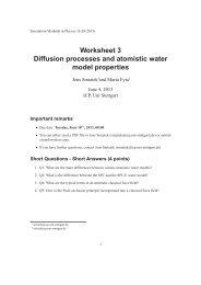
Simulation Methods in <strong>Physics</strong> I<br />
MD in NVE and NVT ensembles<br />
Implementing different thermostats<br />
Fatemeh Tabatabaei, Marcello Sega ∗<br />
1. 12. 2010<br />
ICP, Uni Stuttgart<br />
This tutorial aims at providing knowledge about Molecular Dynamics simulation techniques<br />
in different ensembles. In the following there is a short introduction about physical quantities in<br />
different ensembles and after that, with some programming, the theoretical concept will be applied.<br />
The tutorial main topics are Microcanonical and Canonical ensembles.<br />
Molecular Dynamics in NVE and NVT ensembles<br />
If a system is ergodic, average quantities computed along the trajectory generated by a MD simulation (i.e.<br />
time averages) at constant number N of particles, volume V and total energy E, are equivalent to ensemble<br />
averages in the microcanonical ensemble. Since in the thermodynamic limit (of a large number of particles),<br />
measurements taken in every ensemble are equivalent, one could naively think that a NV E MD simulation is<br />
all what one needs to simulate any thermodynamic point. In practice, however, simulated systems are usually<br />
too small <strong>for</strong> this to happen, and even in the case when they are big enough, it can be complicated to find<br />
out which energy value E is the correct one to simulate the desired thermodynamic point. If, <strong>for</strong> example, we<br />
are interested in a given density and temperature, it is easier to simulate the coupling to an external thermal<br />
bath (hence implementing a canonical, NV T ensemble), than guessing the correct energy. In other cases,<br />
some of the system parameters might not be known a priori. Many algorithms have been devised to simulate<br />
different ensembles like the isothermal-isobaric NpT one (used when the density of the system is unknown) or<br />
the grand-canonical ensemble (µV T ) (where the chemical composition of the system is unknown).<br />
In this tutorial you will learn how to use two different implementations of a thermostat <strong>for</strong> MD simulations,<br />
simulating two different systems. The first system represents a barrier potential. In this system we exercise two<br />
methods <strong>for</strong> thermalizing the system and consequently obtaining constant temperature (NV T ). The first one<br />
is called the Andersen thermostat, in which a constant temperature can be achieved by coupling the system to<br />
a heat bath and the second is called the Nosé-Hoover thermostat. In this method, the motion of the particle<br />
is coupled to a chain of thermostats. The equations of motion are integrated using an explicit time-reversible<br />
algorithm that might look a little bit complicated at first sight. These two methods will be explained more in<br />
detail in the later parts of this tutorial.<br />
The second system represents a Lennard-Jones liquid. With this system we exercise another method to<br />
obtain constant temperature, called Langevin thermostat. In summary, in this tutorial we discuss three<br />
different methods to sample the canonical ensemble.<br />
1 Barrier Crossing<br />
Consider the motion of a single particle in the following external potential (ɛ ≥ 0):<br />
∗ sega@icp.uni-stuttgart.de<br />
1
⎧<br />
⎨ ɛAx 2 x ≤ 0<br />
U(x) = ɛ(1 − cos(2πx)) 0 ≤ x ≤ 1<br />
⎩<br />
ɛA(x − 1) 2 x ≥ 1<br />
(1)<br />
Homework 1 (1 point)<br />
1. As a first task, derive an expression <strong>for</strong> A, so that the <strong>for</strong>ce and its derivative to be continuous, and<br />
make a sketch of the energy landscape.<br />
1.1 System Setup<br />
A program is provided, which integrates the equations of motion of the particle starting at x(t = 0) = 0<br />
using several methods while applying the “barrier potential” equation (1). First inspect the code readdat.c.<br />
This file contains all the in<strong>for</strong>mation required <strong>for</strong> the generation of our system. A description of the input<br />
parameters is provided in the shell script Run/run.sh. You will have to change the setup parameters in that<br />
file in a later part of the tutorial.<br />
The program provides the following methods including two different ensembles:<br />
1. NVE ensemble which can be achieved with a “No thermostat” system.<br />
2. The Andersen thermostat providing an NVT ensemble.<br />
1.2 NVE ensemble<br />
Using this method, a system with constant energy is provided. Try to predict what would you expect the<br />
phase space trajectories (i.e. curves in the 2D position-momentum space, in case of a single particle) to look<br />
like in the case of no thermostat.<br />
Compile the code using make, then change the path to folder Run and run the code launching ./run.sh to<br />
get the data output <strong>for</strong> NVE ensemble.<br />
Remark : In order to switch the code <strong>for</strong> an NVE ensemble, change the value of “CHOICE” in the run.sh to<br />
"1". The other “CHOICE” values <strong>for</strong> other methods are commented in run.sh as well.<br />
Homework 2 (2 points)<br />
1. Set the temperature to T = 0.05. This is a low temperature and the system behaves like a harmonic<br />
oscillator. Explain why it is so.<br />
Notice: Think about the potential function.<br />
2. Plot the phase space distribution. Explain why the phase-space distribution looks like a circle.<br />
3. Plot the phase-space trajectories at two other values of T like T = 1.5 and T = 4.0. What do you<br />
observe? Explain.<br />
1.3 Constant temperature ensemble<br />
In the thermostat proposed by Andersen the system is coupled to a heat bath that keeps the system at the<br />
desired (average) temperature. The coupling to a heat bath is represented by stochastic impulsive <strong>for</strong>ces that<br />
act occasionally on randomly selected particles. These stochastic collisions with the heat bath transport the<br />
system from one constant-energy shell to another. Between stochastic collisions, the system evolves at constant<br />
energy according to the normal Newtonian laws of motion. The stochastic collisions ensure that all accessible<br />
constant-energy shells are visited according to their Boltzmann weight.<br />
All thermostats have in common that they transfer heat, sometimes momentum or angular momentum to<br />
or from the system. Obviously, the total energy then loses its property as a control parameter of the system<br />
(i.e. it is not anymore a conserved quantity). This means that it is no longer obvious whether our simulations<br />
is on the safe side on numerical grounds (Note that Nosé and Hoover <strong>for</strong>mulated a method, the Nosé-Hoover<br />
2
thermostat, where the energy accounting of the heat bath is realized by one (or more) fictitious particle, which<br />
is propagated like the real particles of the system and this particle acts as a reservoir of the energy <strong>for</strong> the<br />
heat bath. Then, the total energy of the extended system is again a conserved quantity, and again a control<br />
parameter is available).<br />
The integration of the Andersen thermostat in integrate-and.c is not implemented yet.<br />
implement the algorithm yourself according to the following steps:<br />
You should<br />
1. Start with an initial set of positions and momenta {r N (0), p N (0)} and integrate the equations of motion<br />
<strong>for</strong> a time ∆t. For this you can use the Velocity-Verlet algorithm.<br />
2. A particle is randomly selected to undergo a collision with the heat bath. The probability that a particle<br />
is selected in a time step of length ∆t is ν∆t. <strong>Here</strong> ν is the collision frequency and specifies the strength<br />
of the coupling to the heat bath. <strong>Here</strong> you should use RandomNumber() from file ran_uni<strong>for</strong>m.c.<br />
3. If the particle has been selected to undergo a collision, its new velocity will be drawn from a Maxwell-<br />
Boltzmann distribution corresponding to the reservoir temperature T . For generating a Gaussian distributed<br />
random velocity look at the file ran_uni<strong>for</strong>m.c. Use the function RandomVelocity() (To read<br />
more about the algorithm <strong>for</strong> Andersen thermostat see [1] ).<br />
Homework 3 (2 points)<br />
1. Make plots <strong>for</strong> the phase space distribution at low temperature T = 0.05 <strong>for</strong> different values coupling<br />
parameters. What do you observe?<br />
2. Compare the phase space distribution generated by the Andersen thermostat with the phase space<br />
distribution you obtained <strong>for</strong> NV E ensemble in the last homework.<br />
3. The relation between the reservoir temperature T and the kinetic energy per particle is<br />
k B T = m 〈 v 2 α〉<br />
, (2)<br />
where m is the mass of the particle and v α is the α-th component of its velocity. This is often used<br />
to measure the temperature in a microcanonical MD simulation. However, the condition of constant<br />
temperature is not equivalent to the condition that the kinetic energy per particle is constant. In a<br />
canonical ensemble of the finite system, the instantaneous kinetic temperature T k fluctuates. Running<br />
the code provides you the instantaneous kinetic temperature in every time step in temp.dat. Plot the<br />
data and explain what you see.<br />
4. When running the code you will get the “Averaged temperature” as an output. Make a record of the<br />
average temperature <strong>for</strong> the two methods. Change the “NSTEP” parameter (number of time steps<br />
in the run) and see if any meaningful change happens towards getting a value closer to the reservoir<br />
temperature. Comment on this.<br />
5. By changing the value of the temperature, investigate at which temperature the particle is able to cross<br />
the energy barrier in two methods. Remark: Crossing the barrier here means to find the density of<br />
the particle at the top of the barrier area to be non-zero.When you run the simulation you will get the<br />
density distribution output. So investigate the density distribution at different temperatures.<br />
2 Lennard-Jones liquid<br />
Now we consider the second system, a Lennard-Jones liquid (you should already be familiar with it from<br />
previous tutorials) that consists of N particles located in a 3D cubic simulation box with edge length L, which<br />
interact with each other via the Lennard-Jones potential. In this case we employ the Langevin thermostat in<br />
order to simulate the canonical ensemble.<br />
3
2.1 Langevin Thermostat<br />
In the Langevin thermostat, at each time step every particle is subject to a random (stochastic) <strong>for</strong>ce and to<br />
a friction (dissipative) <strong>for</strong>ce. There is a precise relation between the stochastic and dissipative terms, which<br />
comes from the so-called fluctuation-dissipation theorem, and ensures sampling of the canonical ensemble. The<br />
equation of motion of particle i is thus modified:<br />
ma i = F i − mγv i + W i (t) (3)<br />
<strong>Here</strong> γ is a friction coefficient with units of t −1 and W i is a random <strong>for</strong>ce that is uncorrelated in time and<br />
between particles, and is characterized by its variance:<br />
2.2 Velocity-Verlet <strong>for</strong> Langevin thermostat<br />
〈W i (t) · W j (t ′ )〉 = δ ij δ (t − t ′ ) 6k B mT γ (4)<br />
The modified Velocity-Verlet algorithm <strong>for</strong> a Langevin thermostat is as follows<br />
where the G i is the total <strong>for</strong>ce: G i = F i + W i .<br />
Homework 4 (1 points)<br />
x i (t + ∆t) = x i (t) + ∆tv i (t)(1 − ∆t γ 2 ) + ∆t2<br />
2m G i(t) (5)<br />
v i (t + ∆t) = v i(t)(1 − ∆t γ 2 ) + ∆t<br />
2m (G i(t) + G i (t + ∆t))<br />
(1 + ∆t γ 2 ) (6)<br />
1. Derive Eq. (6) using Eq (3). Remember that, according to the Verlet algorithm (See Lennard-Jones<br />
liquid tutorial), we have v(t + ∆t) = v(t) + a(t)+a(t+∆t)<br />
2<br />
∆t.<br />
2.3 System Setup<br />
A program is provided (in folder program2) which integrates the equation of motion <strong>for</strong> the N fluid particles.<br />
There are two major elements in this code. First is the <strong>for</strong>ce initialization at each time step that adds in the<br />
random <strong>for</strong>ces, W i . The second is a slight modification to update equations in the integrator to include the<br />
effect of γ.<br />
Homework<br />
You should modify the integration algorithm in such a way that gives us a constant temperature according<br />
to the Langevin dynamics, according to Eqs. 5,6. The updates <strong>for</strong> the velocities should be done in two<br />
half integration steps like in the usual Velocity-Verlet. After finishing the implementation <strong>for</strong> the integration<br />
compile the code.<br />
Remark: you can compile the code using this syntax : gcc -O3 -o lan_thermo lan_thermo.c -lm -lgsl<br />
Homework 5 (2 points)<br />
1. To get a quick help run ./lan_thermo -h. Then you find out which arguments correspond to the<br />
parameters. For example, to specify the number of particles and the number of steps use:<br />
./lan_thermo -N 256 -ns 10000.<br />
2. When running the code you will get an output file data.txt: the first 5 columns are time-step, time,<br />
potential, kinetic and total energy. Integrate 10000 steps with γ = 1.0 and γ = 0.0 Plot the<br />
potential, kinetic and total energy <strong>for</strong> these two systems as a function of time in a single figure. Explain<br />
what do you see. Which of them are constant and which of them fluctuates? Why ?<br />
3. Make a plot of the kinetic temperature (with γ=1.0). That can be done by plotting the 7th column of<br />
the data output. Explain what do you see.<br />
4
Figure 1: Typical mean square displacement of a Lennard-Jones fluid. The solid lines represent the balistic<br />
and diffusive behaviors.<br />
Since you have per<strong>for</strong>med MD simulations, you also obtained in<strong>for</strong>mation about the dynamics of the system.<br />
The next task is to analyse the velocity autocorrelation function, C(τ), (VACF), and the mean square<br />
displacement ∆r 2 (t) (MSD) which are defined as follows:<br />
C(τ) = 〈⃗v(t) · ⃗v(t + τ)〉 (7)<br />
∆r 2 (τ) = 〈|⃗r(t + τ) − ⃗r(t)| 2 〉 (8)<br />
The VACF shows the timespan of the correlation between the velocities of a particle. This in<strong>for</strong>mation may<br />
be useful in interpreting the shapes of MSD(τ) curves. At very small time intervals τ the motion is ballistic,<br />
while after more random kicks from neighbours, particles lose the memory of their original direction of motion<br />
which is manifested by VACF(τ) ≈ 0 and the motion becomes diffusive.<br />
In the program2 folder you can find the diffusion.c code, which analyzes both the MSD (-m option) or<br />
the VACF (-v option) given a series of frames. The programs reads its data as from stdin and expects either<br />
only coordinates or velocities. Supposing you saved a set of configurations (0.xyz,. . . ,1000.xyz,. . . ), starting<br />
from an equilibrated one, you can provide the proper input to the analysis code with such a command line:<br />
cat ?.xyz ??.xyz ???.xyz | grep "^16" | awk ’{print $2,$3,$4}’ |<br />
./diffusion -m -b 100 -n 216 -d 3 > msd.dat<br />
the xyz files are first concatenated in temporal order, then grep is used to select the lines with in<strong>for</strong>mation<br />
about position and velocities. Last, awk is used to print the 2nd, 3rd and 4th column, where the coordinates<br />
are stored. The output is then passed to the analysis code, specifying a window of 100 frames, 216 particles<br />
per frame, and 3 dimensions, and saved in the msd.dat file.<br />
2.4 Homework (2 points)<br />
1. Plot the MSDs and VACFs at two different densities (e.g., 0.5 and 0.8) As an example see figures 1 and<br />
2. Note that MSD should be plotted on a log-log scale.<br />
2. Explain the different behavior of the VACFs at the two densities.<br />
3. Explain the different regimes in the MSD.<br />
5
Figure 2: Typical velocity autocorrelation function of a Lennard-Jones fluid.<br />
References<br />
[1] Molecular Simulation of Fluids, R. J. Sadus, Elsevier Science Publishers pp. 304 - 309<br />
6