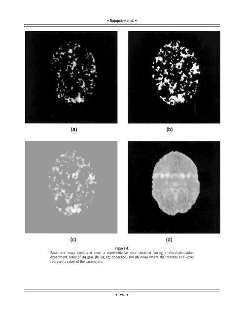
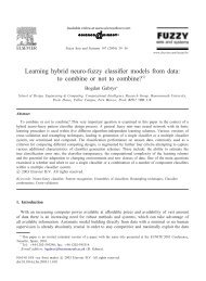
Rajapakse et al. Figure 4. Parameter maps computed over a representative slice obtained during a visual-stimulation experiment. Maps <strong>of</strong> (a) gain, (b) lag, (c) dispersion, and (d) noise where the intensity at a voxel represents values <strong>of</strong> the parameters. 292
HDMF <strong>of</strong> f<strong>MRI</strong> Time-Series TABLE II. Comparison <strong>of</strong> <strong>hemodynamic</strong> parameters <strong>of</strong> the largest activated region and nonactivated region in a visual-stimulation experiment, using the t-test* Region Gain Lag (s) Dispersion (s 2 ) Noise Mean SD Mean SD Mean SD Mean SD Activated region 0.053 0.024 4.504 0.915 4.721 2.628 0.050 0.032 Nonactivated region 0.000 0.004 0.577 2.308 0.471 2.356 0.013 0.031 Significance (P-value) P 0.001 P 0.001 P 0.001 P 0.169 * Significance <strong>of</strong> the comarison in the tests is given as P-values. effectiveness depends on its ability to avoid false alarms in the correction process. Hence, the above S/N ratio gives a quantitative measure <strong>for</strong> the improvement achieved in the <strong>hemodynamic</strong> correction. Figure 3 shows the f<strong>MRI</strong> <strong>time</strong> courses obtained by averaging the <strong>time</strong>-series over the voxels <strong>of</strong> the largest activation blob and the fitted model wave<strong>for</strong>ms using each HDMF. Note the drift in our data, which was corrected by using a linear dummy variable in the regression <strong>analysis</strong>. The actual <strong>time</strong> courses seen in the plots <strong>for</strong> the different models are different because the sizes <strong>of</strong> the detected regions slightly differ in some cases. Poisson and Gamma functions gave similar fits, while Gaussian functions gave a symmetrical fit at the rise and fall <strong>of</strong> stimulations. Maps <strong>of</strong> gain, lag, dispersion, and noise values obtained in the particular slice in the visual-stimulation experiment are shown in Figure 4, where the intensities <strong>of</strong> the voxels represent the values <strong>of</strong> each parameter. The parameters <strong>of</strong> the largest region and the nonactivated voxels with their standard deviations are given in Table II. (The <strong>hemodynamic</strong> parameters <strong>for</strong> nonactivated voxels do not have any meaning, but result as a by-product <strong>of</strong> the <strong>analysis</strong>.) The differences <strong>of</strong> the <strong>hemodynamic</strong> parameters measured over the activated and nonactivated voxels were compared using t-tests. The significances or P-values <strong>of</strong> their differences <strong>of</strong> lag and dispersion at the two sites are also shown. Data obtained in six EPI experiments were analyzed similarly as above, and improvements in the activity patterns were seen with <strong>hemodynamic</strong> correction <strong>for</strong> all data sets. The results <strong>of</strong> <strong>hemodynamic</strong> correction applied to all four slices <strong>of</strong> a representative experiment are shown in Figure 5. Note the improvement <strong>of</strong> the activations or z-maps with <strong>hemodynamic</strong> correction. Table III shows the characteristics <strong>of</strong> the largest activated region with and without <strong>hemodynamic</strong> correction and using multiple regression <strong>analysis</strong> <strong>for</strong> the third slice <strong>of</strong> the sequence. Space-dependence <strong>of</strong> <strong>hemodynamic</strong> parameters In order to find the dependence <strong>of</strong> <strong>hemodynamic</strong> parameters on various brain sites during a sensory simulation, the images taken at six sagittal levels (W 1 ...W 6 ) in a representative word-discrimination experiment were analyzed. Figure 6 shows the detected activations <strong>of</strong> the corresponding slices with and without <strong>hemodynamic</strong> correction, assuming a Gaussian HDMF. The largest activation regions <strong>of</strong> six slices were compared among one another with t-tests <strong>for</strong> any discrepancies in lag and dispersion values. Significance <strong>of</strong> the differences or P-values is shown in Table IV. As seen in Table IV, the lag and dispersion values computed over some regions showed significant differences, while others were statistically similar. Intersubject variability <strong>of</strong> <strong>hemodynamic</strong> parameters To investigate the intersubject variability <strong>of</strong> the <strong>hemodynamic</strong> parameters, three data sets (V 1 ,V 2 , and V 3 ) at the same axial level, obtained while 3 different subjects separately per<strong>for</strong>med the same visual-stimulation task, were analyzed. In all 3 cases, activations appear in the visual cortex, as seen in Figure 7, both with and without <strong>hemodynamic</strong> correction. The <strong>hemodynamic</strong> parameters <strong>of</strong> the largest activated regions <strong>of</strong> different subjects were compared using t-tests and their significances are shown in Table V. The lag values were significantly different between V 1 and V 3 and between V 2 and V 3 , whereas the dispersions were statistically different between V 1 and V 2 and between V 1 and V 3 . DISCUSSION In the absence <strong>of</strong> proper understanding <strong>of</strong> the coupling between cerebral neuronal activity and associated <strong>hemodynamic</strong>s, the linear convolution models 293