Extraction of Passive Device Model Parameters ... - ETRI Journal

Extraction of Passive Device Model Parameters 

Using Genetic Algorithms 

Ilgu Yun a) , Lawrence A. Carastro, Ravi Poddar, Martin A. Brooke, Gary S. May, Kyung-Sook Hyun, and Kwang Eui Pyun 

The extraction of model parameters for embedded passive 

components is crucial for designing and characterizing 

the performance of multichip module (MCM) substrates. 

In this paper, a method for optimizing the extraction of 

these parameters using genetic algorithms is presented. 

The results of this method are compared with optimization 

using the Levenberg-Marquardt (LM) algorithm used in 

the HSPICE circuit modeling tool. A set of integrated resistor 

structures are fabricated, and their scattering parameters 

are measured for a range of frequencies from 45 MHz to 5 

GHz. Optimal equivalent circuit models for these structures 

are derived from the s-parameter measurements using each 

algorithm. Predicted s-parameters for the optimized equivalent 

circuit are then obtained from HSPICE. The difference 

between the measured and predicted s-parameters in the 

frequency range of interest is used as a measure of the accuracy 

of the two optimization algorithms. It is determined 

that the LM method is extremely dependent upon the initial 

starting point of the parameter search and is thus prone to 

become trapped in local minima. This drawback is alleviated 

and the accuracy of the parameter values obtained is 

improved using genetic algorithms. 

Manuscript received November 27, 1999; revised January 20, 2000. 

a) Electronic mail: iyun@etri.re.kr 

I. INTRODUCTION 

As electronics technology continues to develop, there is a 

continuous need for higher levels of system integration and 

miniaturization. For example, in many applications, it is desirable 

to package several integrated circuits (ICs) together in 

multichip modules (MCMs) to achieve further compactness and 

higher performance. Passive components (i.e., capacitors, resistors, 

and inductors) are an essential requirement for many 

MCM applications [1]. A significant advantage of MCM technology 

is the ability to embed large numbers of these passive 

components directly into the substrate at low cost. Such an arrangement 

provides further advantages in component miniaturization, 

power consumption, reliability, and performance. 

It is common for high frequency systems to include filters 

with specifications into the gigahertz range. In order to successfully 

design passive filters at such high frequencies, the behavior 

of the passive components that comprise the filter must be 

modeled accurately up to those frequencies. Recently, computeraided 

design tools such as HSPICE [2] have become indispensable 

in IC design. Accurate circuit simulation using HSPICE 

is dependent on both the validity of the device models and the 

accuracy of the values used as model parameters. Therefore, 

the extraction of an optimum set of device model parameter 

values is crucial to characterizing the precise relationship between 

the device model and the measured behavior. Even if the structure 

of a model is valid, it could lead to poor simulation results if 

model parameters are not extracted properly. 

In this paper, a method for optimizing the extraction of these 

parameters using genetic algorithms (GAs) is presented [3]. GAs 

are a set of guided stochastic search procedures based loosely on 

the principles of genetics. To investigate the use of GAs for the 

optimization of parameter extraction in passive devices operated 

38 Ilgu Yun et al. ETRI Journal, Volume 22, Number 1, March 2000

at high frequencies, a set of integrated passive structures were 

fabricated, and their scattering parameters were measured for a 

range of frequencies from 45 MHz to 5 GHz. Optimal equivalent 

circuit models for these structures were derived from the s- 

parameter measurements. Predicted s-parameters for the optimized 

equivalent circuit were then obtained from HSP ICE. 

The difference between the measured and predicted s- 

parameters in the frequency range of interest is used as the measure 

of the accuracy of the optimization results. 

Conventional optimization techniques such as the Levenberg-Marquardt 

(LM) method [4], which is used by HSPICE 

for parameter extraction, are often subject to becoming trapped 

in local minima, leading to suboptimal parameter values. 

GAs represent an effective method for determining the global 

minimum and are less dependent upon the initial starting point 

of the search. Here, we compare optimization using the LM algorithm 

to optimization using GAs. It is determined that drawbacks 

of the LM method are alleviated, and the accuracy of the 

parameter values obtained is improved using GAs. 

Probe Pad 

Probe Pad 

20 Uncoupled Line Building Blocks 

... 

(a) 

(b) 

Shielded Stub 

Probe Pad 

10 Uncoupled Line Building Blocks 

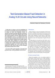
II. TEST STRUCTURE DESCRIPTION 

Three different types of passive devices were considered in 

this study. These test structures are shown in Fig. 1. The first 

structure is simply a straight-line resistor with probe pads on its 

ends. This structure is needed to characterize basic uncoupled 

material parameters including self resistance, inductance, and 

capacitance. The second test structure is an interdigitated capacitor. 

This type of device is used in a wide variety of circuits, 

including resonators, oscillators, and filters to perform functions 

such as DC blocking, frequency filtering and impedance 

transformation. The final test structure is a three-dimensional 

solenoid inductor made using a low-temperature cofired ceramic 

(LTCC) process [1], [5]. 

The resistor and capacitor test structures were built using 

Ti/Au deposited on a 96 % alumina substrate. An electron beam 

evaporation system was used to deposit 0.04 um of titanium 

followed by a 0.2 um layer of gold. The thin layer of titanium 

was used to improve adhesion of the gold to the substrate. 

Following deposition, the resistors were defined using standard 

photolithography and etch back techniques. The photoresist 

was hard-baked for five minutes at 125 °C in order to stabilize it 

before etching. The gold was etched in a heated KCN solution 

for one minute, followed by a buffered oxide etch to remove 

the titanium. Due to the surface roughness of the substrate (approximately 

+/− 1.5 um), the edges of the resistor were jagged, 

but the lines were continuous. All processing was done at the 

Georgia Tech Microelectronics Research Center. 

The LTCC inductor structure was designed within the Cadence 

Virtuoso design environment. A custom technology file 

(c) 

Fig.1. Schematic three test structures: (a) straight-line resistor; 

(b) interdigitated capacitor; and (c) LTCC inductor. 

for a 12-layer process was developed, and a process design rule 

compliant test structure coupon was fabricated at the National 

Semiconductor Corporation LTCC fabrication facility. The size 

of the completed coupon was approximately 2.25" × 2.25". 

Each layer of ceramic tape was specified to be 3.6 mils thick 

with a dielectric constant of 7.8. The metal lines were drawn to 

be 10 mils wide, and the vias were a diameter of 5.6 mils. 

III. MODELING SCHEME 

High frequency analysis of complex geometrical structures is 

required to investigate their electrical performance in a frequency 

range of interest. This analysis is especially important to determine 

the effects of unwanted spurious couplings and resonances which 

can greatly affect the overall system response. Analysis such as this 

is usually only achievable through the use of electromagnetic or 

RF/microwave simulation tools. The derivation of equivalent circuit 

models is very useful to designers who would 

ETRI Journal, Volume 22, Number 1, March 2000 Ilgu Yun et al. 39

1 2 

Probe Pad Building Block 

R_pad = 0.1E-3 Ohm 

L_pad = 0.2E-10 H 

C_pad = 0.1E-14 F 

Uncoupled LineBuilding Block 

1 2 

C_cou = 1.2E-15 F 

R_pad = 0.08 Ohm 

L_pad = 1E-11 H 

C_pad = 2.7E-15 F 

1 2 

1 2 

(a) 


1 2 


1 2 

Shielded Stub Building Block 

1 

2 

3 

2 

1 3 

1 2 

1 2 


L_pad = 1.2E-11 H 

C_pad = 3.6E-15 F 

C_cou = 1.2E-15 F 


L_pad = 1E-11 H 

C_pad = 2.9E-15 F 

C2 = 3.3E-15 F 

R = 0.6 Ohm 

L = 1E-10 H 

C = 7.1E-15 F 

(b) 



1 

1 2 

2 

R_pad = 1E-3 Ohm 

L_pad = 1.8e-10 H 

C_pad = 3.1e-13 F 

1 2 

C_cou = 1.2E-15 F 

R_pad = 1E-3 Ohm 

L_pad = 8.3E-11 H 

C_pad = 2.8E-14 F 

1 2 

(c) 

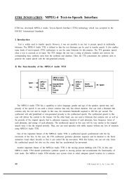
Fig. 2. Building blocks with associated circuit topologies and model parameters for (a) the straight-line resistor; (b) the interdigitated 

capacitor; and (c) the LTCC inductor. 


like to incorporate the complex behavior of these structures in a 

system level circuit simulation. However, the process of obtaining 

lumped models from these simulators is a slow and computationally 

challenging task. 

The modeling procedure implemented here involves determining 

a set of fundamental building blocks for the passive 

structures and then characterizing test structures comprised of 

combinations of those blocks [6]. The test structures are measured 

up to a desired frequency, and the electrical contribution to 

the overall response by the building blocks can then be determined. 

Equivalent circuits of each of the building blocks are 

then extracted using a hierarchical extraction procedure that 

will be described. Simulation of the derived circuit in a standard 

SPICE-compatible circuit simulator then provides the desired 

prediction of electrical behavior. Test structure models are verified 

experimentally by comparing the predicted electrical response 

with the measured response. 

1. Test Structure Characterization 

The test structures described in Section II above were measured 

using standard network analysis techniques. For high frequency 

measurements, an HP 8,510 C network analyzer was 

used in conjunction with a Cascade Microtech probe station 

and ground-signal-ground configuration probes. Calibration 

was accomplished using a supplied substrate and the linereflect-match 

(LRM) calibration method. After calibration was 

completed, s-parameters were obtained for each of the test 

structures at 201 frequency points between 45 MHz and 5 GHz. 

This data was stored with the aid of computer data acquisition 

software and equipment. 

2. Device Model Parameter Extraction 

For passive device structures, it is desirable to predict their 

electrical behavior in a standard circuit simulator. In order to 

accomplish this, circuit models for each of the defined building 

blocks need to be extracted. The fundamental circuit for the 

building blocks is based on the partial element equivalent circuit 

(PEEC) [7] which has been used extensively for interconnect 

analysis [8] and general three-dimensional high frequency 

structure simulation [9]. Coupling behavior is represented by 

the coupling capacitance between center nodes of the two 

PEEC circuits, as well as by mutual inductances between the 

left upper and left lower branch inductors in the model, and 

likewise for the right hand side. These circuits represent models 

for the building blocks only. The test structure circuits are comprised 

of many of the building block circuits connected in accordance 

with the structure geometry. The various circuit models 

and parameters for the different building blocks are shown 

in Fig. 2. 

After the circuit models for the different building blocks 

were obtained, the extraction of the circuit model parameters 

was achieved using two different optimization techniques. The 

first method chosen was the Levenberg-Marquardt (LM) algorithm 

[10]. Since the LM algorithm is built into HSPICE, all 

LM-based optimization and simulations were done using the 

HSPICE simulator on a Sun Sparc 20 workstation. Since the 

starting point or initial guesses for the circuit parameters were 

crucial for achieving convergence, an initial optimization was 

done assuming that each test structure was comprised of just 

one building block, utilized repetitively across the length of the 

structure on a per square basis. The initial guesses for the circuit 

parameters were derived by converting the measured s- 

parameters to z-parameters, and then dividing by the number of 

blocks used in order to extract the valid R, L, and C, values for 

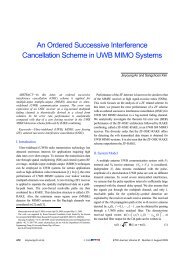
the circuit model. Figure 3 shows a flow chart for the s- 

parameter extraction procedure. 

However, since small changes in the initial guesses often led 

to non-convergence or incorrect optimization results, another 

optimization method which used genetic algorithms (GAs) was 

investigated. GA optimization was performed by software written 

in ANSI standard C++, and was compiled for use in the 

UNIX environment. HSPICE circuit simulations were still 

needed to obtain s-parameter data to complete GA optimization. 

GAs represent a guided stochastic approach to optimization 

which establishes a parallel search of the solution space. Since 

GAs use a large population of trial solutions, they can explore 

many regions of the search space simultaneously. Therefore, 

GAs are insensitive to initial guesses, and they are less likely to 

become trapped in local optima compared to conventional 

optimization methods. Further details on both the LM algorithm 

and GAs are provided in the following section. 

IV. PARAMETER OPTIMIZATION METHODS 

The equivalent circuit model parameter values required by 

the HSPICE simulator are usually obtained by curve fitting the 

model equations to device measured data. This curve fitting is 

accomplished using nonlinear least squares optimization techniques. 

Optimization is the process by which the set of model 

parameter values which best fit the data are selected. This optimum 

parameter set is created by adjusting an initial estimate 

of model parameter values using an iterative process. The 

process continues until simulated output data matches the actual 

measured output data within specified tolerances. In short, 

given a set of measured data, the optimizer solves for a set of 

model parameters which produce simulated data that optimally 

approximates the measured data. 


Define test structure geometry and 

building blocks 

Fabricate test structures 

Measure s-parameters for test structure 

purely gradient descent when the Marquardt scaling parameter 

is very large, whereas the LM method is equivalent to the 

Gauss-Newton method when the Marquardt scaling parameter 

is zero. 

The objective function of LM algorithm is 

⎡ ( ) − ⎤ 

( ) = ( 1, 

2 ,..., 

) = ∑ 

m 

i 

fi 

X Fmeas 

Fo 

X X x x x ⎢wi 

i ⎥ (1) 

n 

i= 

1 ⎣ Fmeas 

⎦ 

2 

Extract circuit models for each building 

blocks using PEEC 

Device Model Parameter Optimization 

1) LM algorithm 

2) Genetic Algorithms 

Obtain device model parameters 

Simulate s-parameters 

using HSPICE 

Fig. 3. Flow chart for s-parameter extraction. 

1. Levenberg-Marquardt Algorithm 

The optimization method used in the HSPICE simulator is 

the well-known Levenberg-Marquardt (LM) algorithm implemented 

with the Marquardt scaling parameter to prevent unexpected 

deviation of the parameter values. The LM search 

method is a combination of steepest descent and the Gauss- 

Newton method. 

Gradient descent is a commonly used search method where 

parameters are moved in the opposite direction to the error gradient. 

Each step down the gradient results in smaller errors until 

minimum error is achieved. However, simple gradient descent 

suffers from slow convergence, in particular when a minimum 

is approached. Another commonly used method is the gradient 

with momentum that updates parameters proportionally to a 

running average of the gradient. In general, this technique can 

decrease the probability of becoming trapped in local minima. 

Nevertheless, the final iterations of the gradient with momentum 

method are still not effective when approaching a solution. 

The Gauss-Newton method provides better convergence properties 

near the solution. However, at a point away from the solution, 

this method suffers from the fact that prescribed the direction 

may not be a descent direction, and the associated inverted 

Hessian matrix may not exist. 

In the LM algorithm, steepest descent is used initially to approach 

the solution, and then the Gauss-Newton method is used 

to refine the solution. During this search, the Marquardt scaling 

parameter becomes very small, but increases if the solution starts 

to deviate. If this happens, the LM technique optimizer becomes 

where X = (x 1 , x 2 , ..., x n ) are the model parameters to be extracted, 

n is the total number of the model parameters, F i meas is 

the measured value of the ith model parameter, m is the total 

number of measurements, f i (X) is the simulated value of the ith 

point, and w i is a weight factor for the ith measured data point 

(used for giving higher significance to a given data point). 

Therefore, the HSPICE optimizer finds the vector X of the device 

model parameters that minimizes F o (X). 

2. Genetic Algorithms 

Genetic algorithms (GAs) refer to a family of computational 

models inspired by evolution. In the last few years, GAs have 

started to be explored for several applications in industry [11], 

[12]. These algorithms encode a potential solution to a specific 

problem on a simple chromosome-like binary data structure 

and apply recombination operators to these structures so as to 

preserve critical information. An implementation of a genetic 

algorithm begins with a population of (typically random) 

chromosomes. To implement a GA, the set of parameters to be 

optimized are first mapped onto a set of binary strings, with 

each string representing a potential solution. The GA then manipulates 

the most promising strings in searching for improved 

solutions. A GA typically operates iteratively through a simple 

cycle of four stages: 1) creation of a population of strings, 2) 

evaluation of each string, 3) selection of the best strings, and 4) 

genetic manipulation to create a new population of strings. The 

process for optimizing passive device model parameters using 

GAs is shown in Fig. 4. 

The genetic manipulation includes three genetic operations 

—reproduction, crossover, and mutation—to search the optimal 

solution in the entire search space. Using these operations, GAs 

can search through large, irregularly shaped spaces effectively, 

requiring only the information of the objective function. This is 

a desirable characteristic, considering that the majority of commonly 

used search techniques require not only the complete information 

of the objective function but also derivative information, 

continuity of the search space. 

In coding genetic searches, binary strings are typically used. 

One successful method for coding multiparameter optimization 

problems is concatenated, multiparameter, mapped, fixed-point 


Initial population 

P1 

1 0 0 0 1 1 

O1 

1 0 0 0 0 0 

Measure model Parameters 

HSPICE Simulation 

Simulate model Parameters 

crossover point 

P2 

0 1 1 1 0 0 

crossover point 

O2 

0 1 1 1 1 1 

Error 

Criteria ? 

yes 

Fig. 6. Illustration of the crossover operation. 

no 

Genetic Algorithms 

- Reproduction 

- Crossover 

- Mutation 

Extract device model 

parameters 

1 0 1 1 0 1 

1 0 1 1 1 1 

Generate new population 

Fig.7. Illustration of the mutation operation. 

Fig. 4. Optimization process for device model parameters using GAs. 

1 0 1 1 0 1 1 1 

1st parameter = 4.2 

range [2, 5] 

precision = 0.2 

2nd parameter = 7 

range [0, 15] 

precision = 1 

Fig. 5. Example of multiparameter coding. 

coding [3]. If x ∈ [0, 2 b ] is the parameter of interest (where b is 

the number of bits in the string), the decoded unsigned integer 

x can be mapped linearly from [0,2 b ] to a specified interval 

[U min , U max ]. In this way, both the range and precision of the 

decision variables can be controlled. To construct a multiparameter 

coding, required single parameters can simply be 

concatenated. Each coding may have its own sub-length (i.e., 

its own U min and U max ). Figure 5 shows an example of a 2- 

parameter coding with four bits in each parameter. The ranges 

of the first and second parameters are 2-5 and 0-15, respectively. 

The string manipulation process employs the aforementioned 

genetic operators to produce a new population of individuals 

(called offspring) by modifying the genetic code possessed 

by members of the current population (called parents). 

Reproduction is the process by which strings with high fitness 

values (i.e., good solutions to the optimization problem under 

consideration) receive larger numbers of copies in the new 

population. A popular method of reproduction is elitist roulette 

wheel selection [13]. In this method, those strings with large 

fitness values F i are assigned a proportionately higher probability 

of survival into the next generation. This probability distribution 

is determined according to 

P 

select i 

= n 

F 

∑ 

i 

j = 1 

Thus, an individual string whose fitness is n times better than 

another will produce n times the number of offspring in the 

subsequent generation. Once the strings have reproduced, they 

are stored in a mating pool awaiting the actions of the crossover 

and mutation operators. 

The crossover operator takes two chromosomes and interchanges 

part of their genetic information to produce two new 

chromosomes (Fig. 6). After the crossover point has been randomly 

chosen, portions of the parent strings (P1 and P2) are 

swapped to produce the new offspring (O1 and O2) based 

upon a specified crossover probability. Mutation is motivated 

by the possibility that the initially defined population might not 

contain all of the information necessary to solve the problem. 

This operation is implemented by randomly changing a fixed 

number of bits every generation based upon a specified mutation 

probability (Fig. 7). Typical values for the probabilities of 

crossover and bit mutation range from 0.6 to 0.95 and 0.001 to 

0.01, respectively. Higher mutation and crossover rates disrupt 

good “building blocks” (schemata) more often, and for smaller 

populations, sampling errors tend to wash out the predictions. 

For this reason, the greater the mutation and crossover rates and 

the smaller the population size, the less frequently predicted 

F 

(2) 


Table 1. Genetic algorithm parameters. 

Parameters 

Value 

Crossover Probability 0.9 

Mutation Probability 0.01 

Population Size 8 

Chromosome Length 

80 bits 

solutions are confirmed. 

In this study, the genetic algorithms have been implemented 

to extract the passive device circuit model parameters for the 

test structures described above using the following fitness function 

(F fit ): 

1 

= 

1+ ∑ − 

Ffit 

2 

( ymeas 

ysim 

) 

n 

where n is the number of s-parameter measurements taken, 

y meas are the actual s-parameter measurements, and y sim are the 

simulated s-parameters found using HSPICE. The probabilities 

of crossover and mutation were set to 0.9 and 0.01, respectively 

(see Table 1). A population size of 8 was used in each generation. 

Each of the eight device model parameters were encoded 

as a 10-bit string, resulting in a total chromosome length of 80 

bits. The optimization procedure was stopped after 100 iterations 

or when F fit was within a predefined tolerance. 

V. RESULTS AND DISCUSSION 

The optimization results using the LM algorithm in the 

HSPICE optimizer and GAs for the three test structures described 

in Section II are presented here. Each structure requires 

the extraction of eight passive device values from s-parameter 

measurements. The root mean square error (RMSE) between 

the measured and simulated s-parameters has been calculated 

for each optimization method. 

For the extraction of the passive device model parameters in the 

straight-line resistor, 20 different sets of parameters were used as 

the initial starting points for the LM algorithm. These initial sets of 

parameters were randomly selected using 10 % deviation from a 

previously analyzed set of parameters which had converged to a 

solution. Among the 20 simulations, only three converged to a solution. 

Table 2 shows the results of extracting the passive device 

model parameters for the straight line resistor using the LM algorithm 

and GAs. The results illustrate that the LM algorithm can be 

trapped in local minima, and the use of GAs can improve the accuracy 

of the model parameter values. 

(3) 

Table 2. Optimization results for the straight-line resistor. 

HSPICE Optimizer results 

GA result 

Parameter run1 run2 run3 GA_run 

C_cou 1.52E−14 1.63E−13 5.15E−14 2.19E−14 

Rsq 5.38E−02 1.00E−02 3.04E−02 4.83E−02 

Lsq 1.13E−15 9.36E−12 9.36E−12 9.32E−12 

Csq 2.72E−15 2.59E−16 2.61E−15 2.70E−15 

C_cou2 1.00E−15 6.23E−11 7.75E−11 9.22E−11 

R2sq 9.85E−02 1.37E−01 1.15E−01 9.80E−02 

L2sq 8.88E−12 1.15E−12 1.03E−12 9.32E−13 

C2sq 3.35E−17 2.46E−15 8.98E−17 1.20E−17 

RMSE 1.50E−03 1.40E−03 1.40E−03 1.20E−03 

Table 3. Optimization results for the interdigitated capacitor. 


GA result 

Parameter run1 run2 run3 run4 GA_run 

C_cou 1.00E−15 1.00E−15 1.00E−15 1.00E−09 4.40E−16 

R_pad 1.54E−01 1.50E−01 1.59E−01 1.70E−01 5.67E−02 

L_pad 1.54E−11 1.50E−11 1.59E−11 1.20E−11 8.99E−11 

C_pad 3.54E−15 3.50E−15 3.59E−15 3.20E−15 3.59E−15 

Rsq 1.55E−01 1.55E−01 1.55E−01 1.39E−01 1.88E−01 

Lsq 8.87E−12 8.87E−12 8.87E−12 9.15E−12 9.42E−12 

Csq 2.76E−15 2.76E−15 2.76E−15 2.25E−15 2.51E−15 

RMSE 1.13E−03 1.58E−03 1.29E−03 2.03E−03 5.81E−04 

Similar results were found for the interdigitated capacitor test 

structure (see Table 3). In this case, 30 sets of randomly generated 

initial model parameters were used for the LM algorithm, 

and a solution was found for only four of these. The model parameter 

values found using GAs were much more accurate 

compared those found by means of the LM method. 

Table 4 shows the results of extracting the passive device 

model parameters for the LTCC inductor. In this case, 20 sets 

of randomly generated initial model parameters were used for 

the LM algorithm, and a solution was found for ten of these 

cases. From these results, it was found that the LM algorithm 

yields a large variation in the extracted model parameters. 

For example, C_cou varies from 10 −15 to 10 −10 F, and Rsq varies 

from 10 −3 to 10 −6 ohms. However, since GAs can explore 

the search space more effectively, a single solution representing 

the global optimum is found using this method. 


Table 4. Optimization results for the LTCC inductor. 


GA result 

Parameter run1 run2 run3 run4 run5 run6 run7 run8 run9 run10 GA_run 

C_cou 1.36E−10 1.00E−15 1.00E−15 1.00E−15 5.75E−10 1.28E−10 8.36E−11 8.98E−11 1.00E−15 9.23E−11 6.90E−10 

R_pad 1.00E−06 1.00E−06 1.00E−06 1.00E−06 1.00E−06 1.00E−06 1.00E−06 1.00E−06 1.00E−06 1.00E−06 1.03E−16 

L_pad 5.68E−10 2.80E−10 3.01E−10 2.96E−10 5.99E−10 5.67E−10 5.52E−10 5.53E−10 2.95E−10 5.54E−10 6.45E−10 

C_pad 4.03E−13 4.31E−13 4.35E−13 4.29E−13 4.06E−13 4.04E−13 4.05E−13 4.04E−13 4.20E−13 4.04E−13 3.11E−13 

Rsq 1.00E−06 3.18E−03 1.00E−06 1.00E−06 1.83E−03 1.00E−06 1.00E−06 1.00E−06 1.00E−06 1.00E−06 3.40E−03 

Lsq 5.94E−12 6.56E−11 6.25E−11 6.37E−11 1.74E−12 6.21E−12 8.72E−12 8.28E−12 6.40E−11 8.11E−12 8.64E−12 

Csq 1.00E−17 2.90E−15 1.46E−15 2.90E−15 1.00E−17 1.00E−17 1.00E−17 1.00E−17 4.80E−15 1.00E−17 2.35E−17 

RMSE 1.70E−03 1.49E−03 1.31E−03 1.32E−03 1.33E−03 2.49E−03 1.32E−03 1.31E−03 1.32E−03 1.66E−03 8.98E−04 

VI. CONCLUSION 

The extraction of circuit model parameters for the three passive 

device test structures using genetic algorithms has been investigated 

and compared with optimization using the Levenberg- 

Marquardt algorithm used in the HSPICE circuit simulation program. 

Results indicate that GAs tend to provide improved accuracy 

and are better in finding global optima, whereas the LM 

method is extremely sensitive to the initial starting point of the 

parameter search and easily trapped in local optima. However, 

GAs are generally slower and the number of GA iterations and 

the optimum set of GA parameters must be ascertained empirically. 

Thus, a trade-off exists between computational time and 

achieving acceptable accuracy in optimizing model parameters. 

Nevertheless, GAs appear to show much promise in this area. 

ACKNOWLEDGMENT 

The authors would like to thank the National Science Foundation 

(Grant No. DDM-9358163) and the Georgia Tech Packaging 

Research Center (NSF Grant No. EEC-9402723) for support 

of this research. 

REFERENCES 

[1] R. Brown and A. Shapiro, “Integrated Passive Components and 

MCMs: The Future of Microelectronics,” Proc. Int’l. Conf. Exhibition 

Multichip Modules, April 1993, pp. 287–94. 

[2] Hspice Users Manual, Meta Software, May 1996. 

[3] D. Goldberg, Genetic Algorithms in Search, Optimization, and 

Machine Learning, Addison Wesley, 1989. 

[4] J. Zhang, Z. Yang, and L. Zhang, “A Scheme for Extracting Transient 

Model Parameters,” Proc. 4th Int’l. Conf. Solid-state and Integrated 

Circuit Tech., October 1995, pp. 287–91. 

[5] M. O’Hearn, “LTCC Technology: VCO in Low Temperature Co- 

Fired Ceramics Technology,” Elektronik, Vol. 45, No. 20, October 

1996. 

[6] R. Poddar, E. Moon, M. Brooke, and N. Jokerst, “Accurate, Rapid, 

High Frequency Empirically Based Predictive Modeling of Arbitrary 

Geometry Planar Resistive Passive Devices,” IEEE Trans. 

Comp. Pack. & Manufac. Tech. B, Vol. 21, No. 2, May 1998. 

[7] A. Ruehli, “Equivalent Circuit Models for Three Dimensional 

Multiconductor Systems,” IEEE Trans. Microwave Theory Tech., 

Vol. MTT-22, March 1974. 

[8] H. Heeb and A. Ruehli, “Three-Dimensional Interconnect Analysis 

Using Partial Element Equivalent Circuits,” IEEE Trans. Cir. 

& Sys., Vol. 39, No. 11, November 1992. 

[9] A. Ruehli and H. Heeb, “Circuit Models for Three-Dimensional 

Geometries Including Dielectrics,” IEEE Trans. Microwave Tech., 

Vol. 40, No. 7, July 1992. 

[10] D. Marquardt, “An Algorithm for Least-Squares Estimation of 

Nonlinear Parameters,” J. Soc. Ind. Appl. Math., Vol. 11, 1963, pp. 

431–441. 

[11] E. Rietman and R. Frye, “A Genetic Algorithm for Low Variance 

Control in Semiconductor Device Manufacturing: Some Early 

Results,” IEEE Trans. Semi. Manufac., Vol. 9, May 1996, pp. 223– 

228. 

[12] S. Han and G. S. May, “Using Neural Network Process Models to 

Perform PECVD Silicon Dioxide Recipe Synthesis via Genetic 

Algorithms,” IEEE Trans. Semi. Manufac., Vol.10, No. 2, May 

1997, pp. 279–287. 

[13] J. F. Frenzel, “Genetic Algorithms,” IEEE Potentials, Oct. 1993, 

pp. 21–24. 

Ilgu Yun received the B.S. degree in electrical 

engineering from Yonsei University, Seoul, Korea, 

in 1990, and his M.S. and Ph.D. degrees in 

electrical and computer engineering, from Georgia 

Institute of Technology, in 1995 and 1997, 

respectively. He was previously a postdoctoral 

fellow in microelectronics research center at the 


Georgia Institute of Technology. He is now a senior research staff in 

Electronics and Telecommunications Research Institute, Taejon, Korea. 

His research interests include reliability and parametric yield modeling 

for III-V compound semiconductor devices, optoelectronic devices and 

high speed embedded passive components and interconnect of integrated 

modules, and process modeling, control, and simulation applied 

to computer-aided manufacturing of integrated circuits. He is currently 

a member of IEEE Electron Device and Reliability Society. 

Lawrence A. Carastro was born in Miami, 

Florida. He received the B.E.E. and the M.S. 

degrees in electrical engineering from the Georgia 

Institute of Technology in 1995 and 1997 respectively. 

He is currently pursuing his Ph.D. 

degree in electrical engineering also at the 

Georgia Institute of Technology. His research 

areas include analog/mixed signal IC design, 

analog to digital converter design, and passive device modeling methodology. 

He is currently working as a research assistant for Dr. Martin 

A. Brooke at the Georgia Institute of Technology since 1995. He also 

designed, built, and manages his wife’s (Sheri) high-end beauty salon 

business. 

Ravi Poddar received The B.S. Degree in electrical engineering with 

highest honors in 1991, the M.S. degree in 1995, and Ph.D. degree in 

1998 from Georgia Institute of Technology, Atlanta, Georgia, USA. His 

research interests include statistical modeling and yield prediction, 

computer-aided design and simulation of integrated circuits, transistor 

modeling, predictive modeling and characterization of integrated passive 

devices and interconnect, and high-speed automated testing. He is 

currently a CAD engineer at Integrated Device Technology, Duluth, 

Georgia, USA. 

Martin A. Brooke received the B. E. (elect.) degree (1st Class Honors) 

from Auckland University, New Zealand, in 1981, and the M.S. and 

Ph.D. in electrical engineering from the University of Southern California, 

Los Angeles, in 1984 and 1988, respectively. His doctoral research 

focused on reconfigurable analog and digital integrated circuit 

design. He is currently the Analog Device Career Development Professor 

of Electrical Engineering at the Georgia Institute of Technology, Atlanta, 

Georgia, USA, and is developing electronically adjustable parallel 

analog circuit building blocks that achieve high levels of performance 

and fault tolerance. His current research interests are in high-speed, 

high-precision signal processing. Current projects include development 

of adaptive neural network and analog multipliers and dividers, precision 

analog amplifiers, communications circuits, and sensor signal 

processing circuitry. To support this large analog and digital systems research, 

he actively pursues systems level circuit modeling research. He 

has developed software that reduce the complexity of large analog electronic 

system models to a user specified tolerance. Prof. Brooke won 

the only 1990 NSF Research Initiation Award given in the analog signal 

processing area. 

Gary S. May received the B.S. degree in electrical 

engineering from the Georgia Institute of 

Technology in 1985 and the M.S. and Ph.D. degrees 

in electrical engineering and computer 

science from the University of California at 

Berkeley in 1987 and 1991, respectively. He is 

currently an Associate Professor in the School of 

Electrical and Computer Engineering and Microelectronics 

Research Center at the Georgia Institute of Technology. 

His research is in the field of computer-aided manufacturing of integrated 

circuits, and his interests include semiconductor process and 

equipment modeling, process simulation and control, automated process 

and equipment diagnosis, and yield modeling. Dr. May was a National 

Science Foundation “National Young Investigator,” and is Editor-in-Chief 

of IEEE Transactions on Semiconductor Manufacturing. 

He was a National Science Foundation and an AT&T Bell Laboratories 

graduate fellow, and has worked as a member of the technical staff at 

AT&T Bell Laboratories in Murray Hill, NJ. He is Chairperson of the 

National Advisory Board of the National Society of Black Engineers 

(NSBE). 

Kyung-Sook Hyun received the B.S. degree in 

physics from Seoul National University, Seoul, 

Korea in 1987, and the M.S. and the Ph.D. degree 

in physics from KAIST, Korea, in 1989 

and 1992, respectively. While working on her 

Ph.D. degree, she worked on the metastabilities 

on hydrogenated amorphous silicon. Since 1994, 

she has been a senior research staff in ETRI involved 

in optoelectronic devices group and researched on the field of 

high-speed optical communication devices. Her research interests include 

the characterization and the development of III-V compound 

semiconductor devices, such as avalanche photodiodes, for high-speed 

application and integrated waveguide optical devices. She is a member 

of the Korean Physics Society and American Physics Society. 

Kwang Eui Pyun received Ph.D. degree in 

electronic engineering from Yonsei university at 

Seoul Korea in 1990. From 1980 to the middle 

of 1981 he was a research assistant of Yonsei 

university in electronic engineering department. 

From the middle of 1981 to 1984 he was a full 

instructor of Korea Naval Academy in electronic 

engineering department. In the middle of 

1984, he joined ETRI to research semiconductor field. From 1984 to 

1992, he was a Senior Technical Staff in Compound Semiconductor 

Department. In 1993 he was dispatched to the electric and electronic 

department of University of Tokyo for one year to do international research 

activities. After returning from Japan, he was in charge of processing 

laboratories including silicon and compound semiconductor 

fields for one year. From 1995 to the middle of 1998, he was in charge 

of Compound Semiconductor Department of ETRI. From the middle of 

1998, he is currently in charge of optical source and detector team. His 

main areas of interest are compound-based processing fields including 

GaAs, InP, especially high frequency and opto-electronic devices.

Extraction of Passive Device Model Parameters ... - ETRI Journal

You also want an ePaper? Increase the reach of your titles

Delete template?

Save as template?