download the full article here - E-International Scientific Research ...

Volume: 3, Issue: 2, 2011 

April – June 2011 

ISSN 2094-1749

Table of Contents 

9. Morphometric Analysis of Third order River Basins using High 

Resolution Satellite Imagery and GIS Technology: Special Reference 

to Natural Hazard Vulnerability Assessment 

………Pradeep K. Rawat, P.C. Tiwari and Charu C. Pant …70 

10. Seaweed Bath Soap Product Formulation and Development 

.........Rogelio M. Estacio ...88 

11. In Vivo Fluorescence Imaging Of Fruit Fly With Soluble Quantum 

Dots 

..........Tapas K. Mandal, Nragish Parvin and Mitali Saha ..101 

12. Biofertilizers in Action: Contributions of BNF in Sustainable 

Agricultural Ecosystems 

………..A.M., Ellafi, Gadalla, , A. and Galal, Y.G.M. ..108 

13. Successional Changes in Herb Vegetation Community in an Age 

Series of Restored Mined Land- A Case Study of Uttarakhand India 

............Shikha Uniyal Gairola, Prafulla Soni ..117 

14. Short-term dynamics of the active and passive soil organic carbon 

pools in a volcanic soil treated with fresh organic matter 

………Wilfredo A. Dumale, Jr., Tsuyoshi Miyazaki, Taku 

Nishimura and Katsutoshi Seki ..128 

15. Rainwater Harvesting, Quality Assessment and Utilization in Region I 

........Adriano T. Esguerra, Antonio E. Madrid, Rodolfo G. Nillo ..145

E-International Scientific Research Journal 

ISSN: 2094-1749 Volume: 3 Issue: 2, 2011 

Morphometric Analysis of Third order River Basins using 

High Resolution Satellite Imagery and GIS Technology: 

Special Reference to Natural Hazard Vulnerability 

Assessment 

Abstract 

Pradeep K. Rawat * , P.C. Tiwari * and Charu C. Pant ** 

* Department of Geography Kumaun University, Nainital, India 

** Department of Geology Kumaun University, Nainital, India 

Email: geopradeeprawat@hotmail.com 

The main objective of the study was to analysis the morphometric parameters of third order sub 

basins (TOSBs) special reference to natural hazard vulnerability assessment through integrated 

GIS database modeling on geo-informatics and morphometry-informatics modules. The Dabka 

River Basin (DRB) constitutes a part of the Kosi Basin in the Lesser Himalaya, India in district 

Nainital has been selected for the case illustration. Geo-informatics module consists of GIS 

mapping for location map, drainage map, drainage order map, lineament map, structural map, 

geological map etc. Morphometric module consists of morphometric analysis for several 

drainage basin parameters include drainage pattern, stream order, stream number, stream 

length, mean stream length, drainage pattern, drainage density, stream frequency, stream length 

ratio, relief ratio, elongation ratio, bifurcation ratio, form factor, circularity ratio and sinuosity 

index. Consequently the morphometric results integrated with geo-informatics parameters to 

assess the natural hazard vulnerability in all third order sub basins (TOSBs) and the final 

integrated results concluded that out of total 23 sub basins maximum 17 sub basins are highly 

vulnerable for several natural hazards whereas only 4 sub basins and 2 sub basins have 

respectively moderate and low natural hazards vulnerability. 

Keywords: GI-Science, Geo-informatics, Morphometry-informatics, Natural Hazards 

Introduction 

Dwarfing all other mountains of the world in sheer height, Himalaya is the youngest mountain 

system, which is still undergoing tectonic movement due to prevailing geological conditions. 

Though each and every part of the world is more or less susceptible to natural calamities, the 

Himalaya due to its complex geological structures, dynamic geomorphology, and seasonality in 

hydro-meteorological conditions experience natural disasters very frequently, especially waterinduced 

hazards (Bisht, 1991; Bora and Lodhiyal, 2010; Rawat et. al., 2011). Although the 

Himalaya is highly vulnerable for all type of hazards such as erosion, land slide, flood in 

70



monsoon period and drought in non-monsoon period (as drying up of natural water springs and 

streams). In the mountain regions, such as, Himalaya, the problems of earthquake and landslides 

or hillslope instability are very common particularly in the geodynamically sensitive belts, i.e. 

zones of boundary thrusts and transverse faults (Valdiya, 1980). The presence of Main Boundary 

Thrust (MBT) and a number of other major and minor faults the study area is tectonically active 

which makes highly vulnerable the area for natural hazards whereas several morphometric 

parameters of river basin accelerating this vulnerability. In order to that present study highlights 

on these morphometric parameters through GIS (Geographical Information Science) database on 

geo-informatics and morphometry-informatics modules. Throughout the study area third order 

sub basins found highly vulnerable for several types of natural hazards and also responsible to 

accelerate the vulnerability for down order river basins. Therefore the study concentrated on 

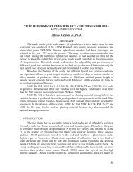
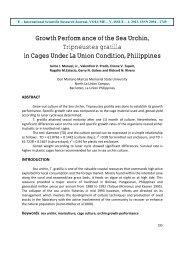
third order sub basins (TOSBs) morphometric analysis. The watershed lies between the latitude 

29°24'09"– 29°30'19"N and longitude 79°17'53"-79°25'38"E in the north-west of Nainital town 

along the tectonically active Main Boundary Thrust (MBT) of Himalaya, India. The region 

encompasses a geographical area of 69.06 km 2 between 700 m and 2623 m altitude above mean 

sea level (Fig.1). 

Dabka Dabka Watershed 

Location Map Map 

I N D I A 

0 100 200 

Km 

Index 

Third order River Basins 

Drainage 

m 

Km 

500 250 0 1/2 1 

Meteorological station 

1:25000 

Figure 1: Location Map 

71



Although in this technology era we are using various digital techniques with the help of 

indigenous software for morphometric analysis but the morphometric studies on river basins 

were first introduction by Horton, 1932 and the idea was later developed in detail by Miller 

1953, Schumm 1956, Melton 1958, Smith 1958, Morisawa 1962, Strahler 1964. In order to that 

a number of other studies have been carried out as a traditional morphometric analysis without 

any scientific application of the morphometric results (Khan, 1998, Nag, 1998; Biswas et al., 

1999; Shrimali et al., 2000; Srinivasa et al., 2004; Chopra et al., 2005 and Nookaratnam et al., 

2005). Whereas the present morphometric analysis advocating a scientific application of the 

results for natural hazard vulnerability assessment which is a major environmental problem of 

the Himlaya because natural hazards in the region cause great loss to life and property and poses 

serious threat to the process of development with have far-reaching economic and social 

consequences. In view of this the proposed work will fill up this highly realized gap and thus will 

have great scientific relevance in the field of natural hazard and risk management in Himalaya 

and other mountainous parts of the world. 

Methodology 

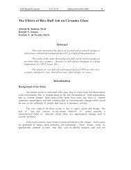
The study comprises mainly two components, (a) lab/desk study and (b) field investigations. 

Geo-structural maps were prepared during field study and details were verified and modified 

with other maps prepared during the lab/desk study. The procedure adopted for morphometric 

analysis and GIS mapping has been outlined in Fig. 2 and describing as below: 

GIS Mapping 

The necessary base maps for morphometric analysis carried out through GIS Mapping using 

Indian Remote Sensing Satellite (IRS-1C) LISS III and PAN merged data of 2010 and SOI 

Topographical Sheets (56 O/7NE and 56 O/7NW) of the area at scale 1:25000 (Fig. 2). These 

required GIS maps are location map, drainage map, drainage order map, lineament map, 

structural map, geological map etc. The satellite images of the study area were registered 

geometrically using SOI Topographical Sheets (56 O/7NE and 56 O/7NW) of the area at scale 

1:25000. For carrying out this important exercise uniformly distributed common Ground Control 

Points (GCPs) were selected and marked with root mean square (rms) error of one pixel and the 

images used were resampled by cubic convolution method. Both the data sets were then coregistered 

for further analysis initially, the LISS and PAN data were co-registered with root 

mean square (rms) error of 0.3 pixel and the output FCC was transformed into Intensity, Hue and 

Saturation (IHS) colour space images. The reverse transformation from IHS to RBG was 

performed substituting the original high-resolution image for the intensity component, along with 

the hue and saturation components from the original RBG images. This merge data product 

obtained through the fusion of IRS –1C LISS – III and PAN was used for the generation of GIS 

mapping through digital image processing techniques supported by intensive ground truth 

surveys were used for the interpretation of the remote sensing data. In order to enhance the 

interpretability of the remote sensing data for digital analysis several image enhancement 

techniques, such as, PCA, NDVI etc. were employed (Fig. 2). 

Morphometric Analysis: The morphometric parameters are calculated based on the formula 

suggested by (Horton, 1945), (Strahler, 1964), (Schumm, 1956), (Nookaratnam et al., 2005) and 

72



(Miller, 1953) given in result section of the article. Morphometric parameters like stream order, 

stream length, bifurcation ratio, drainage density, drainage frequency, relief ratio, elongation 

ratio, circularity ratio and compactness constant are calculated. 

Data Integration and Natural Hazard Assessment: GIS base maps and the morphometric 

results have been integrated and superimposed to identify vulnerability for erosion, landslide and 

flash flood hazards following scalogram modeling approach (Fig. 2). 

Morphometric Analysis and Natural Hazard 

Vulnerability Assessment 

Desk/Lab study 

Field study 

Selection of 

Data sources 

Field Survey 

for Data Sources 

Verification 

Acquisition of 

Topographic Maps 

1:25000 

Acquisition of geo-coded 

data (Liss+Pan) 

1:25000 

GIS Database 

Management (DBMS) 

Morphometry-informatics 

Modeling 

Final Morphometric 

Results 

Geo-informatics 

Modeling 

Preliminary GIS 

Mapping 

Ground truth 

survey on 

Preliminary 

Preliminary 

GIS Mapping 

Final GIS Mapping 

Data Integration and Superimposition 

To Assess Natural Hazards Vulnerability 

Ground truth 

Survey on Final 

Results for 

Verification and 

Figure 2: Procedure Adopted for Study 

73



In scalogram modelling approach (Cruz, 1992), an arithmetic operation was combined with the 

corresponding numerical weights for the vulnerable factors. To assess the combined vulnerability 

level a multiple hazard vulnerability map has been carried out through integration and overlaying 

of all existing natural hazards vulnerability with in third order subbasins (TOSBs). 

Result and Discussion 

Geo-informatics 

Geo-informatics module consists of GIS mapping for location map, drainage map, drainage order 

map, lineament map, structural map, geological map etc. a brief discussion is given as below: 

Drainage Pattern: Drainage network is a significant indicator of the process of landform 

development in a geographical unit. Horton (1932) advocated, a drainage basin is an ideal unit 

for understanding the geo-morphological and hydrological processes and for evaluating the 

runoff pattern of the streams. The geological settings of the area as portrayed by the main steams 

and their tributaries generally control the drainage of the watershed. Generally the rectangular 

drainage pattern has developed at many places in the watershed. The drainage pattern of the 

Lesser Himalayan Ranges is quite different from that of Siwalik Hills falling in watershed. This 

difference in the drainage pattern is mainly due to the presence of active Main Boundary Thrust 

(MBT) in the watershed that separates the Lesser Himalaya from Siwaliks. Dabak river is a Sixth 

order stream includes as many as 495 first, 105 second, 22 third, 5 fourth and 2 fifth order 

streams (Fig. 3 and Table 1). 

Third order Sub-Basins (TOSBs): As discussed introduction and methodological section that 

through out the study area third order sub basins found highly vulnerable for several types of 

natural hazards and also responsible to accelerate the vulnerability for down order river basins. 

Therefore the study concentrated on third order sub basins (TOSBs) morphometric analysis. Fig. 

4 and Table 1 showing that there are total twenty three third order sub basins in the study area 

which all have been selected for comprehensive morphometric analysis. 

Table 1: Number of Streams in different stream orders 

Stream order 

No. Of Stream 

1 st 495 

2 nd 105 

3 rd 23 

4 th 5 

5 th 2 

6 th 1 

74



Dabka Watershed 

Drainage Order 

West Dabka R. 

East Dabka R. 

Dabka R. 

Index 

I. Order Streams 

II. Order Streams 

IV. Order Streams 

V. Order Streams 

0 0.5 1 2 

Km 

1:25000 

III. Order Streams 

Figure 3: Drainage map of the area of present investigation 

VI. Order Streams 

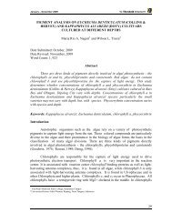
Lineament and Structural Setting: A lineament is a linear feature in a landscape which is 

an expression of an underlying geological structure such as a fault. Typically a lineament 

will comprise a fault-aligned valley, a series of fault or fold-aligned hills, a straight 

coastline or indeed a combination of these features. Fracture zones, shear zones and 

igneous intrusions such as dykes can also give rise to lineaments. Lineament orientations 

are dominantly found in NE to SW and NW to SE orientations in the study area (Fig. 4). 

Geology and Structural Setting: Geologically the study area is located in the southeastern 

extremity of the Krol belt forming outer part of Lesser Himalaya in Kumaun (Auden 1934). 

The watershed encloses rocks of the Blaini-Krol-Tal succession which are thrust over the 

autochthonous Siwalik Group along the Main Boundary Thrust (MBT) of Himalaya. The 

rocks of the area are divisible into Blaini and Krol groups (Rawat and Pant 2007). The 

Blaini Group has been further sub divided into Bhumiadhar, Lariakantha, Pangot and 

Kailakhan formations in an ascending order of succession (Fig. 4) The oldest rocks 

exposed in the watershed comprise quartzwacke, quartzarenite, diamictite, siltstone and 

shale (Bhumiadhar Formation) followed upward by predominantly arenaceous Lariakantha 

75



Formation, which intern is followed by the diamictites, purple grey slates, siltstone and lenticular 

pink siliceous dolomitic limestone of the Pangot Formation. The upper most Kailakhan 

Formation comprises dark grey carbonaceous pyritous slate and siltstone. The Blaini Group 

transitionally grades into the Krol Group. The lower most formation of the Krol Group is 

characterized by argillaceous marly sequence of the Lower Krol Formation (= Krol A). The 

Formation grades upward into purple green slates and yellow weathered dolomites with pockets 

of gypsum of the Hanumangarhi Formation (= Krol B). The Formation constitutes a marker 

horizon in the Krol belt. The Upper Krol Formation (Krol C, D, and E) is characterized by an 

assemblage of dolomitic limestone at the base followed by carbonaceous shales, fenestral 

dolomite showing cross bedding, brecciation and oolites and cryptalgal laminites. The upper 

most part is made up of massive stromatolitic dolomites locally cherty and phosphatic at places. 

The youngest Tal Formation comprises purple green slates interbedded with cross-bedded finegrained 

sandstone and siltstone. The lower most southern part of the watershed comprises 

Siwalik Formation with massive sandstones. 

22 

1 


Third Order Sub-Basins 

2 

3 


Lineaments 

4 

5 

23 

13 

14 

16 

15 

17 

18 


Lineaments 

7 

6 

8 

9 

10 

11 12 21 

Index 

19 

20 

Third order Sub Basins (TOSBs) 

Fourth to Sixth order Basins 

Index 

Index 

Lineaments 

Lineaments 

Third order Sub Third Basins order Sub (TOSBs) Basins 


Existing Land Use 


Geology and Structurl Setting 

After Pant, C.C. (2002) 

Index 

Oak 

Index 

Agricultural Land 

Upper Krol Formation (C,D,E) 

Middle Krol Formation (B) 

Lower Krol Formation (A) 

Kailakhan Formation (Infrakrol) 

Krol 

Group 

Siwalik Group 

Dolerite Dyke 

Faults 

Thrusts 

0 0.5 1 2 

Km 

1:25000 

Pine 

Mixed 

Scrub Land 

Barren Land 

Drainage/River bed 

Third order Sub Basins 

Pangot Formation 

Lariakanta Formation 

Bhumiadhar Formation 

Blaini 

Group 

Third order 

Sub Basins 

Figure 4: Third order Sub Basins, Lineaments, Geology and Land use (Clockwise from upper Left) 

76



Land Use: The forest emerged as the major land use/land cover also in the year 2010. A 

geographical area of 36.77 km 2 , which accounts for nearly 53 % of total area of the watershed, 

has been classified as forests. Due to complexities of terrain and other geomorphic features the 

forests of the watershed are diversified in nature. Out of the total forest 22.20 % (15.33 km 2 ) is 

under mixed forest, 19.56 % (13.51 km 2 ) is under Oak forest, and 11.48 % (7.93 km 2 ) is under 

Pine forests. The hilly and mountainous parts of the watershed are covered with Oak and Pine 

species, whereas, in the lower elevations in the south mixed type of vegetation is very common. 

Agriculture and settlement are now confined to 20.40 km 2 or 29.54 % of the total area. Scrub 

land, barren land and Riverbeds and water bodies respectively extend over 6.22 km 2 (9.01 %), 

3.39 km 2 (4.91 %), 2.28 km 2 (3.30 %) of the total geographical land surface of the study area 

(Fig. 4). 

Morphometry-informatics 

Morphometric module consists of morphometric analysis for several drainage basin parameters 

include drainage pattern, stream order, stream number, stream length, mean stream length, 

drainage pattern, drainage density, stream frequency, stream length ratio, relief ratio, elongation 

ratio, bifurcation ratio, form factor, circularity ratio and sinuosity index as describing following 

sections: 

Drainage basin, drainage divide, and drainage pattern: The entire area of a river basin whose 

runoff drains into the river in the basin is considered as a hydrologic unit and is called a drainage 

basin, watershed or catchment area. The boundary line along a topographic ridge separating two 

adjacent drainage basins is called drainage divide. The DRB possesses a triangular shaped 

catchment area, which develop greater flood intensity at the outlet (at Bagjala). The greater flood 

intensity is because of the analogous length of tributaries and the run off reaches almost at once 

to the outlet. 

Stream Order: The first order streams are those that do not have any tributary. The smallest 

recognizable channels (stream) are called first order and these channels normally flow during 

wet weather (Chow et al., 1988). A second order stream forms when two first order stream join 

and a third order when two second order streams are joined and so on (Strahler, 1964). Where a 

channel of lower order joins a channel of higher order, the channel downstream preserves the 

higher of the two orders and the order of the river basin is the order of the stream draining its 

outlet, the highest stream order in the basin (Chow et al, 1988). It may be noted that Dabka river 

is a sixth order stream and the third to Sixth order streams are perennial and all others are 

ephemeral in nature (Fig. 3 and Table 1). The first order streams (495 numbers) can be identified 

only during monsoon period and stream ordering designates discharge from a drainage network. 

Stream Number: The order wise total number of stream segment is known as the stream 

number. As mention above that Dabak river is a Sixth order stream includes as many as 495 first, 

105 second, 22 third, 5 fourth and 2 fifth order streams (Fig. 3 and Table 1). The data reveals that 

the number of stream segments decreases with increase in stream order. The decrease in the 

number of stream segments is experienced because when a channel of lower order joins a 

channel of higher order, the channel downstream retains the higher of the two orders (Chow et al, 

1988). Table 1 holds excellent the law of stream numbers which states that the number of stream 

segment of each order form an inverse geometric sequence with states the order number (Horton 

77



1945). There is a total of 1945 stream in DRB. Some TOSBs with high proportion of first order 

stream and it may be due to structural weakness present in DRB. For the detailed study of other 

morphometric parameters the TOSBs were taken the number of polygons, perimeter and area of 

23 TOSBs and the remaining portion (23 rd polygon) were determined and the location of TOSBs 

were observe (Fig. 4) and the drainage parameters of the TOSBs were compiled (Table 2). 

Table 2: Results of morphometric analysis of 23 third order basins 

Morphometric parameters 

Sub-basins 

(TOSBs) 

Sub-basin 

Area (Km 2 ) 

Length of Rb (Km.) 

Perimeter (Km.) 

Stream order 

No. of stream 

(Segments) 

Length of 

Stream (Km.) 

Mean Streams 

Length (Km.) 

Streams Length 

Ratio (order) 

Bifurcation Ratio 

Steams Involved in Rb. 

Drainage Density 

(Km/Sq Km.) 

Drainage frequency 

(Streams/sq km.) 

1 

2 

3 

4 

5 

6 

7 

8 

9 

10 

1 13 3.5 0.2692308 6.5 

2 2 1.5 0.75 2.7857 2 14 4 11.33 

1.5 6.4 17.25 3 1 1 1 1.3333 3 

1 8 2 0.25 4 

2 2 1 0.5 2 2 10 2.8 8.67 

1.25 5.3 15.1 3 1 0.5 0.5 1 3 

1 6 1.5 0.25 3 

2 2 0.5 0.25 1 2 8 3.52 13.75 

0.85 4.5 11.3 3 1 1 1 4 3 

1 14 8 0.5714286 4.6667 

2 3 3.5 1.1666667 2.0417 3 17 5.68 9.55 

2.2 12 25 3 1 1 1 0.8571 4 

1 13 5 0.3846154 4.3333 

2 3 1 0.3333333 0.8667 3 16 5.6 16 

1.25 6 14 3 1 1 1 3 4 

1 28 8 0.2857143 4.6667 

2 6 1.5 0.25 0.875 6 34 5.33 18.23 

2.25 10.1 20 3 1 2.5 2.5 10 7 

1 8 2.3 0.2875 4 

2 2 0.5 0.25 0.8696 2 10 5.33 17.34 

0.75 7 17 3 1 1.2 1.2 4.8 3 

1 32 10 0.3125 8 

2 4 2.5 0.625 2 4 36 5.47 15.48 

2.65 11 22.4 3 1 2 2 3.2 5 

1 11 2 0.1818182 5.5 

2 2 1.5 0.75 4.125 2 13 5 14.55 

1.1 10 15 3 1 2 2 2.6667 3 

1 8 2 0.25 4 

2 2 0.5 0.25 1 2 10 1.47 11.35 

1.15 9 16 3 1 1.2 1.2 4.8 3 

78



11 

12 

13 

14 

15 

16 

17 

18 

19 

20 

21 

22 

23 

1 6 1.5 0.25 3 

2 2 0.5 0.25 1 2 8 3.05 12.95 

0.85 6.08 11.1 3 1 0.6 0.6 2.4 3 

1 11 3.2 0.2909091 3.6667 

2 3 1.2 0.4 1.375 3 14 4.52 16.37 

1.15 6.46 13 3 1 0.8 0.8 2 4 

1 13 3.6 0.2769231 3.25 

2 4 1.6 0.4 1.4444 4 17 3.16 10.23 

2.15 12 19.5 3 1 1.6 1.6 4 5 

1 28 10 0.3571429 4.6667 

2 6 5 0.8333333 2.3333 6 34 4.22 9.11 

4.5 19 33 3 1 4 4 4.8 7 

1 9 2.5 0.2777778 4.5 

2 2 1 0.5 1.8 2 11 4.2 14 

1 5.35 13 3 1 0.7 0.7 1.4 3 

1 8 3 0.375 4 

2 2 2.5 1.25 3.3333 2 10 7.37 16.25 

0.8 5.05 11 3 1 0.4 0.4 0.32 3 

1 14 4.5 0.3214286 4.6667 

2 3 1.5 0.5 1.5556 3 17 7.42 12.35 

1.75 7 17.1 3 1 7 7 14 4 

1 24 6.5 0.2708333 3.4286 

2 7 2.2 0.3142857 1.1604 7 31 4.8 16.59 

2.35 12.06 22.2 3 1 2.6 2.6 8.2727 8 

1 6 2.8 0.4666667 3 

2 2 0.4 0.2 0.4286 2 8 4.7 12.94 

0.85 5.12 11.45 3 1 0.8 0.8 4 3 

1 21 8 0.3809524 4.2 

2 5 2.5 0.5 1.3125 5 26 6.76 18.82 

1.7 6.48 18.35 3 1 1 1 2 6 

1 13 5 0.3846154 4.3333 

2 3 1.3 0.4333333 1.1267 3 16 4.88 11.11 

1.8 11.38 19.3 3 1 2.5 2.5 5.7692 4 

1 9 3.8 0.4222222 4.5 

2 2 2.5 1.25 2.9605 2 11 7.88 16.47 

0.85 5.16 13 3 1 0.4 0.4 0.32 3 

1 11 3.5 0.3181818 5.5 

2 2 1.5 0.75 2.3571 2 13 5.8 16.84 

0.95 7.15 14.48 3 1 0.8 0.8 1.0667 3 

Total 35.65 189.59 389.53 135 393 171.5 55.722182 122.97 163.88 464 108.96 308.95 

Ave 1.55 8.243 16.936 5.8696 17.087 7.4565 2.4227036 5.3466 7.1252 20.174 4.7374 13.433 

Stream Length (Lu): Horton’s law of stream lengths states that the mean lengths of streams 

segment of each the order. Generally Lu increases as the order of segment increases. Except the 

TOSBs 7, 8, 9, 10, and 20 Lu decreases as the order of stream segments increases and it 

constitutes about 24% of the TOSBs. The 48 stream orders of TOSBs have Lu less than 1 Km 

79



(57 %), 24 stream orders have a value between 1 and 2 Km for first order streams and for others 

Lu given in Table 2. 

Drainage density (Dd): Drainage density (Dd) is the total length of the stream in a given 

drainage basin divided by the area of drainage basin (Horton, 1932). 

Dd= ∑L/A, 

Where ∑L- total length of the stream, 

A- Area of drainage basin. 

Table 2 depicts the distribution of third order basins under different drainage density groups. The 

Dd value of DRB is 1.82 Km/km 2 . The study of TOSBs revealed that average Dd is 2.67 km/km 2 

and it varies in between 1.47 km/km 2 to 7.88 km/km 2 (Table-2). The highest Dd is for the TOSB 

15, 16, 20, and 22. With a value of 7.37, 7.42, 6.76, 7.88 respectively is situated nearest to the 

highest rainfall occurring region such as Ghughukhan ,Maniya and Binayak. The TOSB 10 with 

lowest Dd value with 1.44, nearer to the lowest rainfall occurring region such as Fathehpur. The 

Table 3 reveals the relationship between rainfall and Dd. At present Ghughukhan rain gauge 

station records highest rainfall. 

The Dd generally increases with rainfall (R) 

Thus Dd ∞ R 

Dd= KXR 

Dd/R = K, where K is a constant and its value is always less than one 

The Dd and R studies reveal that Dd controls runoff following a particular period of 

precipitation and the increasing Dd shows increasing size of mean annual flood. 

Table 3: Relation of rainfall and drainage density (Dd) 

Code 

of 

TOS 

B 

Dd Nearest 

Rain Gauge 

Annual 

mean 

Rainfall 

(mm) 

22 7.88 Ghughukhan 2749.80 

13 3.16 Maniya 2357.10 

10 1.47 Aniya 854.06 

Data 

Recorded 

5Year (2005- 

2010) 

5Year, (2005- 

2010) 

5Year, (2005- 

2010) 

Stream frequency (Df): It is the number of stream segments per unit area (Horton, 1932, 1945). 

The stream frequency, Df = ∑N/A, where N is the number of stream segments and A denotes the 

drainage area. The average Df for DRB is 2.45. The lowest Df value is for the TOSB 8 with a 

value of 8.67 and the highest for the TOSB 20 with a value of 18.82. The frequency value wise 

numbers of TOSBs are tabulated (Table 2).. 

Relation between Drainage Density and Frequency: The relation of Dd and Df revealed that 

the Df is directly proportional to Dd (Table 4) Thus drainage frequency is double the value of 

drainage density and its variation occurs due to rainfall, relief, infiltration rate, and initial 

resistivity of terrain to erosion, total drainage area of the basin and above all the Dd of the basin 

80



itself. The low values of Df indicate poor stream networks and high indicate denser networks in 

the catchment area. 

Stream length ratio (R L ): Stream length ratio is the ratio of mean length of streams of one order 

to that of the next lower order that tends to be constant thorough the successive order of a 

watershed (Horton, 1945). 

The stream length ratio R L = Lu/Lu-1, 

Where Lu is the mean stream length of order u and Lu-1 is the mean stream length of next lower 

order. The average length ratio of TOSBs is 5.35 with highest value of 14.00 for TOSB of 17 

(indicates lower order sources for the next higher order streams) and the lowest 0.32 for the 

TOSBs of 16 & 22 (indicates limited length of lower order streams) Table 2. 

Relief ratio (R h ): The difference in elevation between the highest and lowest points in a basin is 

called basin relief. It indicates the overall steepness of drainage basin and is an ndication of 

intensity of degradation processes operating on slopes of the basin and is ratio between the total 

relief of the basin and its longest dimension parallel to the principal drainage line. R h = H/L b 

Table 4: Relation between Dd & Df 

Sub-basins Drainage Density Drainage Frequency Relation 

(TOSBs) (Km/Sq Km.) (Streams/sq km.) (R=Df/Dd) 

1 4 11.33 2.83 

2 2.8 8.67 3.10 

3 3.52 13.75 3.91 

4 5.68 9.55 1.68 

5 5.6 16 2.86 

6 5.33 18.23 3.42 

7 5.33 17.34 3.25 

8 5.47 15.48 2.83 

9 5 14.55 2.91 

10 1.47 11.35 7.72 

11 3.05 12.95 4.25 

12 4.52 16.37 3.62 

13 3.16 10.23 3.24 

14 4.22 9.11 2.16 

15 4.2 14 3.33 

16 7.37 16.25 2.20 

17 7.42 12.35 1.66 

18 4.8 16.59 3.46 

19 4.7 12.94 2.75 

20 6.76 18.82 2.78 

21 4.88 11.11 2.28 

22 7.88 16.47 2.09 

23 5.8 16.84 2.90 

81



Where H is the total relief and L b is the basin length. The R h value of DRB is 0.173. The low R h 

values are resulted by resistant bedrock and low slope and R h values usually increases with 

decreasing with decreasing drainage area (Table 2). 

Elongation ratio (R e ): It is the ratio of diameter of a circle having the same area as of the basin 

and maximum basin length (Schumm, 1956). The R e is given by 

R e = d/Lb, 

Where d is diameter of a circle having the same area as of the basin, and Lb maximum basin 

length parallel to the principal drainage line. It is a measure of the shape of the river basin and 

the value ranges between 0.6 and 1. Value ranges from 0.6 to 0.8 are regions of high relief and 

the value close to 1.0 are regions of very low relief with circular in shape and are efficient in the 

discharge of runoff than and elongated basin because concentration time is less in circular basins. 

Thus R e values help in flood forecasting. The elongation ratio and shape of basin are given in 

Table 5. 

Table 5: Elongation ratio and shape of river 

Elongation ratio 

Shape of basin 

0.9 Circular 

Elongation ratio 

Shape of basin 



Circularity ratio (R e ): It is the ratio of area of river basin to the area of circle having the same 

perimeter as the basin (Miller, 1935). Like form factor, it is also a dimensionless ratio to express 

outline of drainage basin (Strahler, 1964) and R e is uniform between 0.6 and 0.7 for homogenous 

rock types and 0.40 and 0.5 for quartzitic terrain and is influenced by length and Df of streams, 

geological structures, vegetation, climate, relief and slope of the basin. 

Sinuosity index (S): It is the ratio of channel length and river valley length (Muller, 1968). 

Sinuosity index reveals the topographic and hydraulic conditions of streamlines and it varies 

from 1.1 to 4.0 or more and those having S less than 1.5 called sinuous and with 1.5 or more than 

1.5 are called meandering. Stream channels usually originate in sinuous form, which depends on 

underlying rock structure, climate, vegetation and time. The average Sinuosity index of DRB is 

1.11. 

Data Integration and Natural Hazard Vulnerability Assessment 

The morphometric results have been integrated and superimposed with other GIS base maps to 

natural hazard vulnerability assessment. Mainly three types of natural hazard identified within 

the third order sub basins i.e. erosion, landslide and flash flood hazard. A brief description on 

each type of hazard vulnerability within all the twenty three third order sub-basins given as 

below: 

Erosion Hazard Vulnerability: Increasing first order streams, increasing drainage density and 

frequency are the main morphometric parameter for erosion hazard vulnerability but the frizzled 

geo-ecological parameters (i.e. stressed and crushed geology, active faults and thrust, degraded 

land use pattern and lineaments etc.) are accelerating factor for the hazard vulnerability. 

Therefore out of total 23 sub basins 15 sub basins have high erosion vulnerability whereas 4 sub 

basins found for moderate and 4 sub basins found for low erosion hazard vulnerability (Fig. 5 

and Table 6). 

Landslide Hazard Vulnerability: Although the study area is highly vulnerable for seismic 

landslide activity due to active lineaments such as thrusts (MBT) and number of faults but it 

experienced that the area is equally vulnerable for non-seismic landslide during rainy season 

because of degraded land use pattern whereas the morphometric factors for landslide 

vulnerability are same as for erosion hazard vulnerability. Fig. 5 and Table 6 depicting the spatial 

distribution of the landslide vulnerability within the third order sub basins. Out of total 23 sub 

basins maximum 19 sub basins have high landslide vulnerability whereas only 2 sub basins 

found for moderate and 2 sub basins found for low landslide hazard vulnerability (Fig. 5 and 

Table 6). 

83



22 

4 

1 


Erosion Hazard Vulnerability 

2 

3 

23 

13 

14 

16 

15 

0 0.5 1 2 

Km 

1:25000 

22 

4 

1 


Landslide Hazard Vulnerability 

2 

3 

23 

13 

14 

16 

15 

7 

5 

6 

9 

10 

11 

12 

21 

17 

Index 

High 

19 

18 

20 

7 

5 

6 

9 

10 

11 

12 

21 

17 

Index 

High 

19 

18 

20 

8 

Moderate 

Low 

8 

Moderate 

Low 

22 

4 

5 

6 

7 

1 


Multiple Hazard Vulnerability 

8 

2 

3 

23 

9 

13 

10 

11 

14 

12 

16 

21 

15 

17 

Index 

High 

19 

Moderate 

Low 

18 

20 

22 

4 

5 

6 

7 

1 


FloodHazard Vulnerability 

8 

2 

3 

23 

9 

13 

10 

11 

14 

12 

16 

21 

15 

17 

Index 

High 

19 

Moderate 

Low 

18 

20 

Figure 8: Natural Hazards Vulnerability (Flood, Erosion, and Landslide=Multiple: 

Clockwise from Upper Left to Lowe Left) 

Flood Hazard Vulnerability: Mainly two types of floods are common throughout the Himalaya 

i.e. flash flood and river-line flood which are among the more devastating types of hazard as they 

occur rapidly with little lead time for warning, and transport tremendous amounts of water and 

debris at high velocity. Intense rainfall (IRF) is very frequent cause for flash flood and river-line 

flood in the study area which play a key role for flash flood and river-line flood. The main 

meteorological phenomenon causing intense rainfalls in the region are cloudbursts, stationarity 

of monsoon trough and monsoon depressions. Flash flood in the region cause great loss to life 

and property and poses serious threat to the process of development with have far-reaching 

economic and social consequences. In order to that it is quit important to assess the flood hazard 

vulnerability due to morphometric parameters and geo-environmental factors. The major 

morphometric parameter of flood high hazard vulnerability is decreasing Elongation ratio (R e ). 

The spatial distribution of flood hazard vulnerability with in the third order sub basins suggesting 

that out of total 23 sub basins 6 sub basins have high flood vulnerability whereas only 5 sub 

basins found for moderate and 12 sub basins found for low flood hazard vulnerability (Fig. 5 and 

Table 6). 

84



Table 6: Several Types of Hazards Vulnerability Assessment in 23 third order Sub Basins 

Thir 

d 

orde 

r 

Sub 

Basi 

ns 

Erosion Hazard 

Vulnerability 

(I) 

Different Natural Hazard Vulnerability 

Landslide 

Flash Flood 

Hazard 

Hazard 

Vulnerabilit 

Vulnerability 

y 

(III) 

(II) 

Multiple 

Hazard 

Vulnerab 

ility 

(I+II+III 

) 

1 High High low High 



4 High High Moderate High 




Moderate Moderate Low Modera 

8 

te 


10 

Moderate Moderate High Modera 

te 

11 Low Low Low Low 

12 Low Low Low Low 

13 High High High High 





Moderate Moderate Low Modera 

18 

te 



Moderate Moderate High Modera 

21 

te 



Multiple Hazard Vulnerability: Above study reviles that each third order sub basin not equally 

vulnerable for all three types of natural hazards (Fig. 5 and Table 6). In view of that a combined 

multiple hazard vulnerability map has been carried out through integration and overlaying GIS 

layers of all these three natural hazards vulnerability (i.e. erosion+ landslide+ flood) for each 

third order sub-basin (Fig. 5 and Table 6). This map suggesting that out of total 23 sub basins 

maximum 17 sub basins have high natural hazards vulnerability whereas only 4 sub basins found 

for moderate and 2 sub basins found for low natural hazards vulnerability. 

Conclusion 

Throughout the study area third order sub basins found highly vulnerable for several types of 

natural hazards and also responsible to accelerate the vulnerability for down order river basins. 

Therefore the study concentrated on third order sub basins (TOSBs) morphometric analysis and 

integrated the results with geo-environmental background of the sub basins through GIS database 

85



management system (DMS). The study concluded that each third order sub basin not equally 

vulnerable for all three types of natural hazards. In view of that a combined multiple hazard 

vulnerability map has been carried out through integration and overlaying GIS layers of all these 

three natural hazards vulnerability (i.e. erosion+ landslide+ flood) for each third order sub-basin 

and suggesting that out of total 23 sub basins maximum 17 sub basins have high natural hazards 

vulnerability whereas only 4 sub basins found for moderate and 2 sub basins found for low 

natural hazards vulnerability. 

Acknowledgement 

This study constitutes part of multidisciplinary Collaborated project, Department of Science and 

Technology (D.S.T.) Gov. of India, No.ES/11/599/01 Dated 27/05/2005, “Geo-environmental 

Appriasal of the Dabka Watershed, Kumaun Lesser Himalaya, District Nainital: A Model Study 

for Sustainable Development” funded to Prof. C.C. pant under collaboration of Department of 

Geography and Geology Kumaun University Nainital. Dr. Pradeep Goswami, Senior Scientist, 

Center for climate change, Kumaun University Nainital helped in GIS analysis for which authors 

indebted to him. Thanks to Shri M.S. Bargali, project assistant helped during the intensive field 

work. 

References 

Auden, J.B. 1934. The Geology of the Krol belt. Geol. Soc. India, 67: 357-454. 

Bisht, M.K.S, 1991. Geohydrological and geomorphological investigations of the Dabka 

catchment district Nainital, with special reference to problem of erosion. Unpublished PhD. 

thesis, 37-115. 

Bora, C.S. and L.S. Lodhiyal, 2010. Ecological trends of under canopy species of Eucalyptus 

plantations in Bharbhar and Tarai region of India Central Himalaya. E-International Scientific 

Research Journal, 2 (2): 118-127. 

Biswas, S., S. Sudhakar, and V.R. Desai 1999. Prioritisation of subwatersheds based on 

morphometric analysis of drainage basin: A Remote Sensing and GIS approach, Journal of 

Indian Society of Remote Sensing, 27(3): 155166. 

Chopra, R., R. Dhiman, and P.K. Sharma 2005. Morphometric analysis of subwatersheds 

in Gurdaspur District, Punjab using Remote Sensing and GIS techniques, Journal of 

Indian Society of Remote Sensing, 33(4): 531539. 

Cruz, R.A.D. 1992. The determination of suitable upland agricultural areas using GIS 

technology. Asian pacific Remote Sensing Journal, 5:123-132. 

Melton, M.A. 1958. Correlation structure of morphometric properties of drainage system and 

their controlling agents. J. Geol., 66: 442-460. 

86



Morisawa, M.E. 1962. Quantitative geomorphology of some watershed in the Appalachian 

plateau, Geol. Soc. Bull., 73: 1025-1046. 

Horton, R.E. 1932. Drainage Basin Characteristics. Transfixions of Am. Geophys. Union, 13: 

350. 

Miller, V. C., 1953. A quantitative geomorphic study of drainage basin characteristics in the 

clinch mountain area, Technical report3, Department of Geology, Columbia University. 

Nag, S. K., 1998, Morphometric analysis using remote sensing techniques in the Chaka subbasin, 

Purulia district, West Bengal, Journal of Indian Society of Remote Sensing, 26(12): 69-76. 

Nookaratnam, K., Y.K. Srivastava, V. Venkateswarao, E. Amminedu, K.S.R. Murthy, 2005. 

Check dam positioning by prioritization of microwatersheds Using SYI model and morphometric 

analysis – Remote sensing and GIS perspective, Journal of the Indian Society of Remote 

Sensing, 33(1): 25-28. 

Rawat, Pradeep K., C.C. Pant 2007. Geohydrology of Dabka watershed, using remote sensing 

and GIS”, in Rawat M.M.S and Pratap D. (Ed.), Management Strategy for the Indian Himalayan 

Development and Conservation proceedings of National conference held in Srinagar 

Uttarakhend, India 2007, Trans Media Publication, Srinagar Uttarakhend, India: 161-183. 

Rawat, Pradeep K., P.C. Tiwari, C.C. Pant, A.K Sharama, P.D. Pant, 2011. Climate change and 

its geo-hydrological impacts on mountainous terrain: A case study through Remote Sensing and 

GIS modelling. E-International Scientific Research Journal, 3 (1): 51-69. 

Schumm, S. A., 1956. Evolution of drainage systems and slopes in Badlands at Perth Amboy, 

New Jersey. Geological Society of America, Bulletin, 67: 597-646. 

Shrimali, S.S., S.P. Aggarwal,and J.S. Samra 2001. Prioritizing erosionprone areas in hills using 

remote sensing and GIS – a case study of the Sukhna Lake catchment, Northern India, JAG, 

3(1): 54-60. 

Srinivasa, V. S., S. Govindaonah, and H. G Home 2004. Morphometric analysis of 

subwatersheds in the Pawagada area of Tumkur district South India using remote sensing and 

GIS techniques. Journal of Indian Society of Remote Sensing, 32(4): 351-362. 

Strahler, A. N. 1964. Quantitative geomorphology of drainage basins and channel networks, 

section 4II, In: Handbook of Applied Hydrology, edited by V.T. Chow, McGraw Hill: 439. 

Smith, K.G. 1953. Standard for grading texture of erosional topography, Am. J. Soc., 

5(298):655-668. 

Valdiya, K.S. 1980. Geology of Kumaun Lesser Himalaya. Wadia Institute of Himalaya 

Geology, Dehradun UP.:291. 

87



Seaweed Bath Soap Product 

Formulation and Development 

Abstract 

Rogelio M. Estacio 

Associate Professor 

Don Mariano Marcos Memorial State University, Bacnotan, La Union, Philippines 

The process of making bath soap comprises the following steps: preparation of alkaline 

solution; preparation of seaweed gel, papaya (Carica papaya Linn), atsuete (Bixa orellana Linn) 

and coconut oil as primary ingredients of the product, and mixing these ingredients to produce 

a thick solution, pouring the solution into the molder, cooling and solidifying the solution at 

room temperature, aging , and packaging the end- product. 

The “Seaweed Bath Soap” was an offshoot product of the project entitled “ Seaweed Gel 

Extract Product Formulation and Development.” The soap product containing a mixture of 

seaweed gel, papaya and atsuete extract were brought to the Cagayan Valley Herbal Processing 

Plant.- Philippine Institute for Traditional and Alternative Health Care, Carig, Tuguegarao City 

for bioassay analysis and testing. After which, it was subjected to sensory evaluation by trained 

panelists of Don Mariano Marcos Memorial State University- North La Union Campus. 

Result of the study revealed that the soap product was found to be very much acceptable in its 

overall quality attributes. 

Keywords: Seaweeds bath soap, seaweed gel extract, seaweed product formulation, herbal 

soap, DMMMSU soap 

Introduction 

In the Ilocos Region, seaweeds such as sargassum, gracilaria and eucheuma are abundant. 

Eucheuma is cultured in some parts of the province. Favorable growth of this seaweed is noted 

but still limited to meet the export demand. Sargassum, however, is found washed up on beaches 

in large quantity or floating near shore. Sargassum is found throughout the world’s ocean and 

seas and none is known to be poisonous. It is usually ignored by coastal dwellers and treated as 

waste in the coastal area. 

The objective is to utilize seaweeds such as eucheuma, gracilaria and sargassum seaweeds, and 

turned them into something that would result to a better income opportunity for the fish farmers 

in the region. 

This work can also create employment by putting small and medium enterprises of the product in 

coastal communities as livelihood projects of housewives, out of school youths and jobless 

adults. 

88



Seaweed bath soap is a natural product for cleansing. It is actually a salt that foams. This 

crystalline nature soap is made of seaweed gel extract that is mixed with caustic soda and natural 

oil to produce an opaque, premium bath soap that is mild for sensitive skin. 

The seaweeds eucheuma, gracilaria and sargassum are red-to-brown grass of the sea that 

provide food for man. Aside from being consumed as food these are utilized as raw material in 

the manufacture of industrial products such as alginate, agar and carrageenan. They contain 

protein which help to fight premature aging of the skin by restructuring collagen and generating 

elasticity, skin suppleness which in turn reduces and softens wrinkles. They also contain 

betacarotene to help slow skin aging, treat acne and irritated skin, as well as eczema problems. It 

is also used as detoxifier when it is eaten or applied to the skin. 

The papaya extract is known as an effective skin whitening. Papaya contains vitamins A, that 

benefits the skin through increasing the rate of new cell formation. It also balances and regulates 

skin firmness, tones and improve smoothness. 

The atsuete contains volatile fatty oil with palmitin and traces of stearin alkaloids saponin and 

tannin for homogeneous color of the skin aside from fascinating the product. 

The soap product provides the benefits of exfoliation, cleansing, smoother, healthier looking skin 

that’s is more receptive to moisturizing lotion. Exfoliation is part of natural skin care and the 

secret to smooth, soft healthy looking skin. The seaweed bath soap gently scrubs away dead skin 

and other skin impurities caused by environmental pollutions, sun exposures and stresses of 

everyday life. By using this soap, a younger skin is exposed. It also stimulates blood circulation. 

Analysis showed that the quality attributes of the product such as physical evaluation (texture, 

color, odor, hardness and size) and after-effect evaluation (exfoliation, irritation, freshness, 

irritation, freshness, lather and allergynisity) were very much acceptable . 

Moreover, the soap is cheaper compared to other commercial soap in the market. 

Review of Related Literature 

Seaweeds are rich in vitamins A, B1, B2, B6, Folic acid and Niacin. It supplies 60 trace elements 

and is a primary source of B12 and significant amount of vitamins E and K. It is also an excellent 

source of over 60 minerals, especially potassium, calcium, iodine, magnesium, phosporous iron, 

zinc, manganese (Trono, Gavino, 1989,). 

Seaweed bath soap products hydrate and feed the body through the most vital organ – the skin. 

Our entire skin care bath soap is 100 percent natural, free of dyes, animals-by-products and 

contains no artificial fragrances, making it safe for all skin types. Regular use of seaweed bath 

soap increases the levels of moisture in the skin and promote a healthy glowing complexion. 

Seaweeds contain much larger concentration of what is present in seawater, and in a form, which 

can easily be assimilated, the potassium-sodium content of sea vegetable is usually quite close to 

89



that occurring naturally in human body. Many marine algae are a source of B12, which are rarely 

found in land vegetables. 

Many species of seaweeds contain protein which helps fight premature aging of the skin by 

restructuring collagen and generating elasticity. This increase the skin suppleness which in turn 

reduces and softens wrinkles. Due to its iodine and sulphur amino acid content, seaweeds are 

stimulating, revitalizing and nourishing to the skin. It also offers antibacterial and skin healing 

benefits. 

Objectives 

General: To develop new non-food products from seaweed (eucheuma, greacilaria, and 

sargassum) extract. 

Specific: 

1. To formulate new products, e.g. bath soap with seaweeds extract; 

2. To determine the acceptability of the formulated product; and 

3. To determine the cost and return benefits of the product. 

Expected Output: 

A novel seaweed bath soap that would promote healthy skin. 

Methodology/ Procedure: 

a. Preparation of supplies and materials 

The basic soap ingredients (fats, oil and alkali), seaweed and equipments molder, mixing 

bowl, weighing scale and stirring rod to be used were prepared and set at the processing 

laboratory of DMMMSU-NLUC. Gracilaria spp, Sargassum and Eucheuma seaweeds 

were gathered at the shoreline of Balaoan, La Union. Other raw materials were bought 

locally. The seaweeds were prepared by washing, drying, bleaching, and cooking for 

phycocolloids extraction. 

b. Seaweed bath soap product formulation 

b.1. Bath soap formulation 

90



Table 1. Percentage composition of the ingredients for each seaweed used. 

Treatment Seaweeds Papaya Atsuete 

T 1 45% 35% 20% 

T 2 55% 25% 20% 

T 3 65% 15% 20% 

T 4 conrol Leading brand Leading brand Leading brand 

b.2. Procedure 

1. Dissolve caustic soda flakes in distilled water by continuously stirring until 

completely dissolved and cooled; 

2. Add this to the coconut/oil and mix in a single direction for five minutes; 

3. Add seaweeds extract, papaya and atsuete extract and continue stirring the solution 

for 30-40 minutes; 

4. Pour the solution into the molders; and are left to cool and harden. This is now the 

cooling and solidifying stage; 

5. Afterwhich, remove the soap from the molder and age the soap for 3 to 4 weeks. 

The process will remove the irritation effects of caustic soda; 

6. Finally, the soap is packed for analysis and evaluation. 

c. Representative samples were brought to DOST- Cagayan Valley Herbal Processing 

Plant, Carig, Tuguegarao City for bioassay analysis and testing. 

91



Figure 1. Flow Chart – the step- by- step process of making seaweed bath soap 

7. 

Preparing alkaline solution, seaweed, papaya and atsuete 

extract as ingredients 

Mixing the prepared ingredients through a plastic container 

Stirring the mixed ingredients continuously to 

produce a thick solution 

Pouring the solution into the molder 

Cooling and solidifying the solution at room 

temperature 

Removing the solution to the said molder 

Aging (saponification) the solution, 

Packaging the finish product 

92



d. Test and Evaluation 

1. Sensory evaluation – The formulated bath soap was initially evaluated by 6 panelists who 

tried the product. Below is the rating scale used by the panelists. 

Table 2. Scale Used: 0 – 5 

POINT VALUE RANGE DESCRIPTIVE 

RATING 

5 4.20 – 5.00 Very High 

4 3.40 – 4.19 High 

3 2.60 – 3.39 Moderate High 

2 1.8 – 2.59 Low 

1 0 – 1.79 Very Low 

2. Sampling tools and technique. The panelists, composed of faculty, staff and students 

of the University, used the modified hedonic rating scale to evaluate the products. 

The quality attributes or criteria for evaluation was adopted based on the 

recommendation of the Philippine Institute of Traditional and Alternative Health Care 

for bath soap product. 

3. Data Analysis – Data on the sensory evaluation results were analyzed using the 

analysis of variance (ANOVA) 

Results and Discussion 

A. Acceptability of the seaweed bath soap. 

Sensory evaluation results by the panelists is reflected in Tables 3, 4 and 5. Five (5) 

quality attributes on physical evaluation and five (5) quality attributes on the effect 

of the seaweed bath soap were presented and served as basis for the acceptability 

test of the product. 

Table 3.a. Physical Evaluation. 

Mean response on the different quality attributes of the gracilaria formulated soap. 

Treatment Texture Color Odor Hardness Size Mean Descriptive 

Equivalent 

T 1 4.5 4.5 4.16 4.5 4.16 4.36 Very High 

T 2 4.16 4.83 4.16 4.16 4.5 4.36 Very High 

T 3 3.5 4.0 4.66 4.33 4.16 4.13 High 

T 4 4.35 4.25 4.26 4.26 4.15 4.26 Very High 

93



Table3.b. Effect Evaluation. 

Mean response on the different quality attributes of the gracilaria formulated soap. 

Treatment Exfoliation Irritation Freshness Lather Allergynisity Mean Descriptive 

Equipvalent 

T 1 4.66 4.5 4.33 4.5 4.66 4.53 Very High 

T 2 4.66 4.33 4.0 4.66 4.33 4.39 Very High 

T 3 4.0 3.83 3.66 4.0 4.66 4.03 High 

T 4 4.1 4.15 4.0 4.15 4.25 4.13 High 


Mean response on the different quality attributes of the eucheuma formulated soap 

Treatment Texture Color Odor Hadness Size Mean D. E. 

T 1 4.83 4.83 4.0 4.66 4.66 4.59 VH 

T 2 4.0 4.33 4.5 4.5 4.5 4.36 VH 

T 3 4.33 4.66 4.0 4.5 4.5 4.39 VH 

T 4 4.25 4.25 4.25 4.25 4.25 4.25 VH 

Table 4.b. Effect evaluation. 

Mean response on the different quality attributes of the eucheuma formulated soap. 

Treatment Exfoliaation Irritation Freshness Lather Allergynisity Mean D.E. 

T 1 4.33 4.83 4.5 4.66 4.83 4.63 VH 

T 2 4.0 3.66 3.66 3.83 4.66 3.96 High 

T 3 4.66 4.16 4.16 4.66 4.33 4.39 VH 

T 4 4.16 4.25 4.33 4.25 4.25 4.25 VH 

Table 5.a. Physical evaluation. 

Mean response on the different quality attributes of the sargassum formulated soap. 

Treatment Texture Color Odor Hardness Size Mean D. E. 

T 1 4.83 4.83 4.0 4.66 4.66 4.59 VH 

T 2 4.0 4.33 4.5 4.5 4.5 4.36 VH 

T 3 4.33 4.66 4.0 4.5 4.5 4.39 VH 

T 4 4.25 4.25 4.25 4.25 4.25 4.25 VH 

94



Table 5.b. Effect evaluation. 

Mean response on the different quality attributes of the sargassum formulated soap. 

Treatment Exfoliation Irritation Freshness Lather Allergynisity Mean D.E. 

T 1 4.33 4.83 4.5 4.66 4.83 4.63 VH 

T 2 4.0 3.66 3.66 3.83 4.66 3.96 High 

T 3 4.66 4.16 4.16 4.66 4.33 4.39 VH 

T 4 4.0 4.15 4.25 4.25 4.25 4.18 H 

Result indicated that the mean value of all formulated product is 4.41 which suggests that the 

product is highly acceptable. The five (5) physical quality attributes ( texture, color, odor, 

hardness and size) are indicative to a good bath soap quality attributes considering the “nontraditional” 

materials used in developing bath soap. 

On the other hand, the five (5) effect quality attributes of the seaweed bath soap is very high with 

regards to the acceptability of the soap. The exfoliation, irritation, freshness, lather and 

allergynisity are characteristics of bath soap. The irritation and allergynisity quality attribute is 

very high with a mean value of 4.23 and 4.58, respectively that indicate that the formulated 

seaweed bath soap is considered safe for all skin types. The exfoliation and lather quality 

attributes of the formulated soap is generally acceptable by the panelists with a mean of 4.49 and 

4.36, respectively in which such attributes reflect good quality of the product. 

Meanwhile, the quality attribute of the soap that may need to be improved is the “freshness.” 

Though the product is generally accepted by the panelists, such attribute must be improved for 

acceptance by the general public. 


Mean acceptability of the seaweed bath soap by the panelists on the quality attributes of the 

products. 

Formulated 

soap 

Gracilaria 

soap 

Eucheuma 

soap 

Sargassum 

soap 

Commercial 

soap 

Texture Color Odor Hardness Size Mean Descriptive 

equivalent 

4.05 4.43 4.32 4.33 4.27 4.28 Very high 

4.44 4.60 4.10 4.55 4.66 4.47 Very high 

4.38 4.60 4.16 4.55 4.55 4.44 Very high 

4.29 4.25 4.26 4.26 4.22 4.26 Very high 

95



Table 5.b. Effect Evaluation. 

Mean acceptability of the seaweed bath soap by the panelists on the quality attributes of the 

products. 

Formulated Exfoliation Irritation Freshness Lather Allergynisity Mean D.E. 

soap 

Gracilaria 4.44 4.22 3.99 4.38 4.55 4.31 VH 

soap 

Eucheuma 4.55 4.27 4.05 4.38 4.60 4.37 VH 

soap 

Sargassum 4.33 4.21 4.10 4.38 4.60 4.32 VH 

soap 

Commercial 

soap 

4.09 4.19 4.20 4.22 4.25 4.19 Hgh 

Table 5 presents the mean score of respondents with respect to the three (3) bath soap products. 

Results indicated that all formulated bath soap preparations are highly accepted by the 

respondents with the highest mean of 4.47 and the lowest is 4.26 which has very high descriptive 

equivalent. Irritation and allergynisity are given very high score by the respondents, maybe 

because of the no erythema occurrence to the skin. 

Cost and return analysis 

FIXED CAPITAL Cost/Unit(P) TOTAL AMOUNT(P) 

1 food processor 2,500.00 2,500.00 

1 plastic container 10Lcap 300.00 300.00 

1 stainless casserole 1,000.00 1,000.00 

1 laddle (stainless long 

handle) 

100.00 100.00 

50 pcs plastic molder 50.00 2,500.00 

II. WORKING CAPITAL (one cycle operation) 

Quantity particular Amount 

12 kgs Caustic soda 3,000.00 

50 ltr. Minola oil 5,000.00 

3kg Dried gracilaria 200.00 

1kg Dried atsuete seed 100.00 

1 contract labor 5 days @ 190.00 950.00 

600 pcs. Paper boards 2,040.00 

96



III. TOTAL PROJECT COST 

P17,690.00 

IV. Depreciation Cost per cycle 

Particular Cost Number of Salvage value Depreciation cost 

Services 

Food processor 2,500.00 100 50.00 24.50 

Plastic container 300.00 100 3.00 2.97 

Stainless 

casserole 1,000.00 200 10.00 4.95 

laddle 100.00 200 2.00 

molder 2,500.00 200 50.00 12.25 

Total depreciation Cost P46.67 

Projected Income per cycle 

Total number of production per cycle 

1,200 pcs/cycle 

Selling Price (farm gate) 

P25.00 per piece 

Cost of sale per cycle P 17,690.00 

Total Sales 30,000.00 

Net Income 12,310.00 

Break even price 14.74 

ROI 41 % 

Economic analysis 

The utilization of low grade/rejected/washed-out/highly abundant seaweeds will pave a new area 

of developing alternative livelihood and resource utilization for the benefits of coastal 

communities. 

The basic soap ingredients such as oil and alkaline as well as the equipments can be bought 

locally. The seaweeds can be gathered easily the coastal areas. Thus, the total cost for a single 

operations of the soap making is very minimal and affordable by the producers. The return of 

investment is 41% if price is P25.00/pc. and break even at P14.74/pc. 

Table 6.a. Erythema test 

Skin reaction of test animals after application of test soap samples with code numbers T 1 

gracilaria T 2 gracilaria T 3 sargassum. 

Skin 

Reactions 

S 

C 

O 

R 

E 

F1-1 F1-2 F3-2 

A) erythema 30min 24h 3day 7days 30min 24h 3day 7days 30min 24h 3day 7days 

No 0 

erythema 

- 0/10 0/10 0/10 0/10 0/10 0/10 0/10 0/10 0/10 0/10 0/10 

Very Slight 1 

eryrhema 

1/10 - - - - - - - - - - 

97



Well 

defined 


Moderate to 

severe 


Erythema 

with eschar 

2 

- - - - - - - - - - - 

3 

- - - - - - - - - - - 

4 - - - - - - - - - - - 

Table 6.b Edema test. 

Skin reaction of test animals after application of test soap samples with code numbers T 1 

gracilaria T 2 gracilaria T 3 sargassum. 

Skin 

Reactions 

S 

C 

O 

R 

E 

F1-1 F1-2 F3-2 

A) edema 30min 24h 3day 7days 30min 24h 3day 7days 30min 24h 3day 7days 

No edema 0 - 0/10 0/10 0/10 0/10 0/10 0/10 0/10 0/10 0/10 0/10 0/10 

Very Slight 1 

edema 

- - - - - - - - - - - - 

Well 2 

defined 

- - - - - - - - - - - - 

edema 

Moderate to 3 

severe 

- - - - - - - - - - - - 

edema 

Edema with 

eschar 

4 - - - - - - - - - - - - 

Tables 6.a & 6.b. represent the skin reactions of mature guinea pig (about 4 months old 

male). Results indicated that the formulated bath soap causes one of the ten (1/10) 

animals reacting with very slight erythema which detected within the first 30 minutes 

with reversible reaction during the succeeding periods of evaluation. The skin reaction 

was evaluated in 30 minutes, 24hours, 3days and 7 days for reactions of erythema and or 

edema. 

Table 7. Mean weight (g)/hr of dissolved soap material observed with the seaweed soap 

samples. 

T1-1 (g/hr dissolve) T1-2 (g/hr dissolve) T3-2 (g/hr dissolve) 

14.35 15 16.5 

21.12 18 19.5 

8.59 10 9.5 

Total 44.06 43 45.5 

Mean 14.68 14.33 15.16 

The mean weight (g) lost/hr (14-15g) of dissolution time for soap samples are not comparably 

different, which means that the quality of the formulated soap is almost equal. 

98



Analysis of variance (ANOVA) on the mean score of the panelists on the physical quality 

attributes of the products shows that there were no significant differences; Fc is lesser than Ft. 

But on the effect quality attribute, analysis of variance shows that there is significant difference 

in eucheuma formulated soap (Fc is greater than Ft). 

Summary, Conclusion and Recommendations 

Summary 

The seaweed bath soap product was formulated out of seaweeds, papaya and atsuete extracts 

combined with coconut oil. The use of the local materials as soap ingredient will optimize the 

utilization and increase the current effort of seaweeds farmers. 

A formulation protocol was developed in coming up with the seaweed bath soap product. The 

product was brought to DOST- Cagayan Valley Herbal Processing Plant, Carig, Tuguegarao City 

for bioassay analysis and testing. The product was sensory-evaluated by 10 trained panelists of 

the DMMMSU-NLUC, Bacnotan, La Union. The result indicated that all seaweed bath soap 

preparations including the control are highly acceptable by the respondents. 

Conclusions 

Results indicated the following: 

The seaweed soap product was generally accepted as to its quality attributes, though other factor 

attributes such as freshness shall be improved. 

There are no significant differences with regards to the quality attributes and among soap 

preparations presented for evaluation. 

The application of the soap formulations (gracilaria, sargassum, eucheuma) did not cause skin 

edema in guinea pig during the rest of the evaluation. 

The patch application with test soap samples T 1 gracilaria caused one of the ten(1/10) animals 

reacting with very slight erythema detected within the first 30 minutes with reversible reaction 

detected during the succeeding periods of evaluation. 

Recommendations 

The seaweed bath soap must be tested by a wider consumer group to serve as basis for further 

improvement of the quality attributes of the product; and 

Stability and packaging studies must be undertaken for quality development and standardization 

prospect of the product. 

99



References 

1. http://www.perfects.net/Aoqili-Seaweed-Soap-defat-Soap-All-Natural-5,3-02-barhtml 

2. http://www.aromatic.com/seaweed.html 

3. http://www.ihatecellulite.com/cellulite-seaweed-soap.html 

4. http://www.bluespenoriginals/seaweed.soap.html 

5. http://bathgifts.us/ 

6. http://ezinearticle.com/?slimming-seaweed-soap---Abetter-Alternativeandid=827378 

7. http://soapoperabathshop.blogspot.com/ 

8. http://www.redonbit.com/news/health/819342/seaweed_substance_helps_againsts_ski 

n_cancer/ 

9. http://www.ehow.com/facts_5700892_benefits_seaweed-bath_html 

10. Trono, Gavino, 1989, Field Guide and Atlas of the Seaweed Resource of the 

Philippines. 

Seaweed Bath Soap 

` 

100



In Vivo Fluorescence Imaging Of Fruit Fly 

With Soluble Quantum Dots 

Tapas K. Mandal, Nragish Parvin and Mitali Saha 

Department of Chemistry, National Institute of Technology Agartala, Agartala- 799055, India 

Corresponding address:- 

*Tapas K. Mandal 

Department of Chemistry, 

National Institute of Technology,Agartala-799055,India; 

Cell: +91 8974729766 

E-mail : tps.mndl@gmail.com 

Abstract 

The ability of multi colour fluorescence imaging with water soluble carbon quantum dots 

(WSCQDs) in organisms and biological tissues has been explored using Drosophila 

melanogaster (fruit flies). Here we present strategies to visualize different developmental stages 

and their various internal organs in vivo and in vitro condition with multiple, distinct colors. 

Their viability and growth were not reduced by oral quantum dots ingestion. We demonstrate a 

new methodology in the field of bioimaging by using synthesized water soluble carbon quantum 

dots (WSCQDs) that will bring a revolution in the history of biomedical science. 

Keywords: Noninvasive, bioimaging, carbon, quantum dots, water soluble, fruit fly 

Introduction: 

Exploration of quantum dots in biological systems got attention ever since its discovery. The role 

of WSCQDs, in biological systems and its implications are currently under evaluation primarily 

on the work interfacing chemistry, physics and biology. The emergence of fluorescence carbon 

nanoparticles/ dots shows high potential in biological labeling, bioimaging, and other different 

optoelectronic device applications (Batalov et al., 2009; Selvi et al., 2008; Mochalin and 

Gogotsi 2009). These carbon nanoparticles are biocompatible and chemically inert, (Lim et al., 

2009 ; Kong et al., 2005) which has advantages over conventional cadmium-based quantum dots 

(Medintz, et al., 2005). However, these application of fluorescent carbon nanoparticles are 

poorly studied compared with other carbon or cadmium based materials. In addition, the 

understanding of the uses of fluorescence character in carbon nanoparticle is far from sufficient. 

(Zhou et al., 2007; Zhao et al., 2008). For example, the understand dynamic processes in live 

cells, such as intercellular and intracellular trafficking, microstructure remains unclear. To prove 

these difficult imaging tasks, a robust water soluble QDs are needed. Several synthesis strategies 

have been used, such as surface functionalization with water-soluble ligands (Sun et al., 2006), 

101



silanization (Cao et al., 2007) and encapsulation within block-copolymer micelles (Liu et al., 

2007). Here, we investigated the photo physical properties of water-soluble CQDs prepared by a 

synthesis method based on Common routes in making fluorescent water soluble carbon quantum 

dots followed by oxidation of carbon soot ( collected from waste plant materials burning) with 

nitric acid (Ray et al., 2009). 

We observed that these small carbon particles enter into cells without any further 

functionalization and the fluorescence property of the particles can be used for fluorescencebased 

cell-imaging applications. The ability of multi color fluorescence imaging with WSCQDs 

in organisms and biological tissues has been explored by using Drosophila melanogaster (fruit 

flies). In vivo emission imaging has made detailed study of a biological species by fluorescence 

microscopy. 

Therefore we show all the in vivo images of various internal organs through out the 

developmental phases of Drosophila melanogaster using a new fluorescent material like 

WSCQDs and tally with a control experiment. We successfully acquire in vivo images of the 

developing three larval stages till the adult hood by using the minimally invasive imaging 

modality of ordinary fluorescence microscopy. The whole-body imaging of a probe in real time 

means that the efficacy of therapeutic treatments can be seen directly without the need for any 

invasive procedure. 

Experimental Procedures / Materials and Methods: 

Synthesis of water soluble Carbon Particles: 

Carbon soot 50 mg (collected from burning waste plant materials) was mixed with 30 ml of 5 M 

nitric acid in a 50ml three-necked flask. It was then refluxed at 140 °C for 10 h with magnetic 

stirring. After that, the black solution was cooled and centrifuged at 8000 rpm for 7 min to 

separate out unreacted carbon soot. The light brownish-yellow supernatant was collected, which 

shows green fluorescence under UV exposure. The aqueous supernatant was mixed with acetone 

(water/acetone volume ratio was 1:3) and centrifuged at 16000 rpm for 10 min. The black 

precipitate was collected and dissolved in 30 ml of water. The colorless and nonfluorescent 

supernatant was discarded. This step of purification separates excess nitric acid from the carbon 

nanoparticles. This concentrated aqueous solution, having almost neutral pH, was taken for 

further use. The same synthesis technique was also performed for 18 h of reflux. The supernatant 

obtained from the 18 h reflux, was dark yellow. We weighed the unreacted carbon soot, which 

was removed as precipitate, in order to find out the yield of soluble carbon nanoparticles. 

The weight was ∼50 mg for the 18 h reflux times (yield ∼22%). This solution has particles 

having sizes ranging from 20 to 220nm and is called as-synthesized carbon quantum dots 

(CQDs) (see Scheme 1). Figure-2 shows AFM and TEM images of WSCQDs. 

Fly cultured with water soluble CQDs: 

Flies were of the Canton S strain (obtained from the laboratory of Dr Pradip Singha , 

Department of biological science ,IIT Kanpur) that had been reared in the laboratory for many 

generations. Stocks were maintained in an room temperature at 20- 25°C under a L14:D10 

photoperiod in 250-ml bottles on WSCQDs mixed 60g of a cornmeal–agar medium seeded with 

yeast. Cornmeal agar medium was made according to a recipe modified from (Lewis, 1960). 

102



Agar (8.00g) and 0.5mg WSCQDs mixed water (1000 ml) were added to a saucepan and heated 

until boiling. 50 grams of organic cornmeal, 40g dextrose, 25g dried yeast were mixed together 

and added when the agar was boiling. The mixture was simmered for 5 min and then removed 

from the heat and allowed to cool to at room temperature . 2.5 gms of Nipagin and 9 ml 

propionic acids in 15 ml of 95% ethanol were then added and stirred into the food. 

Flies that were to be used in experiments were reared as follows. Twenty virgins adult were 

assigned randomly to media containing vial. Vials were plugged with cotton wool bungs and 

placed in a room temperature / incubator at 20-25°C under a L14:D10 photoperiod (the lights 

came on at 08:00 GMT). 

Drosophila were treated for two- three days before to lay eggs. These eggs were allowed to grow 

under WSCQDs treated food to complete their life cycle. 

Another set of experiment (control) has done without any WSCQDs, others conditions were 

same like treated and their life cycle was monitored. The organism and their all life cycle stages 

were washed thrice with the sterilized PBS (pH 7.4) for fluorescence microscopy (LEICA 

DC200). 

Fluorescence microscopy: 

Images of life cycle stages of drosophila were captured by using a Leica inverted microscope 

(Leica DC200, Leica microscopy system ltd, CH-9435, Heerbrugg) with an attached RS 

Photometrics Sensys camera, KAF1401E G1. The intensity of fluorescence was quantified by 

using the 488, 561 and 633nm band pass (BP) emission filter functions of the Leica microsystem 

imaging solution software (Leica Q fluoro version V1.0a, Leica microsystem imaging solution 

ltd, Germany). 

Result and Discussion: 

The fruit fly Drosophila melanogaster is one of the most valuable organisms in genetic and 

developmental biology studies. Transgenic methods are in use to image with bleachable organic 

fluorphore or fluorescent protein, full image of all the stages of the life cycle of the living wild 

organism is lacking. WSCQDs have a high emission range fluorescence property. The 

fluorescence property of the particles were used to track their position in cells using a 

conventional fluorescence microscope. We acquire in vivo images of the eggs through all the 

larval stages till adult hood under oral ingestion (figure-3). Figure-4. showed multicolored 

fluorescence images providing clearer internal structure of Drosophila. In contrast, the 

fluorescence signals of the cells without addition of the CQDs were invisible in control 

experiments. Furthermore, these images reveal WSCQDs bind to the cells, but it is nonspecific. 

The possible mechanisms are that the WSCQDs with surface carboxylic acids bind on the 

surface of cells (Jessica et al., 2007; Liu and Vu, 2007). It indicated that the water-soluble CQDs 

bind on the surface of cells. Since the surface of WSCQDs were the functional carboxylic Group 

was free, which can be easily coupled with amine groups the surface cell of an organism, such as 

proteins, peptides and amino acids. In fact, one cell membrane carries numerous proteins and one 

protein typically bind on numerous water soluble CQDs. 

103



We observed the viability rate of the both control and treated organisms were same. While both 

of them completed their life cycle within 12-14 days. Their behavioral pattern is same with the 

normal fly. So WSCQDs does not show any toxic effect during the life cycles of Drosophila). 

Conclusion: 

Before our these experiments a non-invasive method to create an image of a body structure from 

a laboratory animal using relatively simple equipment is not known. Bio–imaging began since 

the discovery of X-rays by Roentgen in 1895. The magnetic resonance imaging (MRI) technique 

has been introduced to overcome the relatively high permeability of X-rays and its deleterious 

effects on biological tissue. The imaging can noninvasively monitor cellular or genetic activity 

and subsequently use the results to track gene expression, the spread of disease, or the effect of a 

new drug in vivo. Our imaging process could give in vivo multicolor fluorescence images. Water 

soluble carbon quantum dots will become key probes for multicolor fluorescence microscopy. It 

is suitable for long term imaging because it is not photo bleaching. Also it has not cytotoxic 

effect. The whole-body imaging of a probe in real time means that the efficacy of therapeutic 

treatments can be seen directly without the need for any invasive procedure. Our approach can be 

used for milligram-scale to bio imaging . These fluorescence imaging process can useful for 

medical applications. These process can obtain in vivo images of cells without any invasive 

surgery. Also these process have the potential in biomedical applications where cadmium-based 

quantum dots show toxic effects. However, synthetic methods of these particles need to be much 

more advanced so that large quantities of these particles with different emission colors were 

easily prepared. 

Acknowledgements: 

T. K. M., N.P. and M.S. are grateful to Prof. R. Gurunath, Prof. S. Sarkar and Prof. B. Prakash, 

IIT Kanpur for providing necessary laboratory facilities. N.P. T.K.M thanks NIT Agartala for 

providing a fellowship. Thanks to Prasenjit Samanta and Santanu Mondal of D.A.V college, 

Kanpur, for helping us. 

References: 

Batalov, A., Jacques, V., Kaiser, F., Siyushev, P., Neumann, P., Rogers, L. J., McMurtrie, R. L., 

Manson, N. B., Jelezko, F. and Wrachtrup, (2009). Low temperature studies of the excited-state 

structure of negatively charged nitrogen-vacancy color centers in diamond. J. Phys. ReV. Lett. 

15;102(19):195506. 

Cao, L., Wang, X., Meziani, M. J., Lu, F., Wang, H., Luo, P. G., Lin, Y., Harruff, B. A., Veca, L. 

M., Murray, D., Xie, S. Y. and Sun, Y. P.(2007). Carbon dots for multiphoton bioimaging. J. 

Am. Chem. Soc. 129, 11318. 

Jessica, P., Ryman-Rasmussen, Nancy, A., Riviere, J.E. and Monteiro-Riviere. (2007). Variables 

Influencing Interactions of Untargeted Quantum Dot Nanoparticles with Skin Cells and 

Identification of Biochemical Modulators. Nano Lett. 7:1344–1348. 

104



Kong, X. L., Huang, L. C. L., Hsu, C. M., Chen, W. H., Han, C. and Chang, H. C. (2005). Highaffinity 

capture of proteins by diamond nanoparticles for mass spectrometric analysis,” Anal. 

Chem. 77, 259-265. 

Lewis, E.B. (1960). A new standard food medium. D. I. S. 34: 117--118. 

Lim, T.S., Fu, C.-C., Lee, K.-C., Lee, H.-Y., Chen, K., Cheng, W.-F., Pai, W. W., Chang, H.-C. 

and Fann, W. (2009). Fluorescence enhancement and lifetime modification of single 

nanodiamonds near a nanocrystalline silver surface. Phys. Chem. Chem. Phys. 14;11(10):1508- 

14. 

Liu, H., Ye, T. and Mao, C. (2007). Fluorescent Carbon Nanoparticles Derived from Candle 

Soot. Angew. Chem. 46 (34), 6473-6475 

Liu, H.Y. ,and Vu, T.Q.( 2007). Quantum Dot Hybrid Gel Blotting: A Technique for Identifying 

Quantum Dot-Protein/Protein-Protein Interactions .Nano Lett. 7:1044–1049. 

Mochalin, V. and Gogotsi, Y.( 2009). Wet Chemistry Route to Hydrophobic Blue Fluorescent 

Nanodiamond. J. Am. Chem. Soc.131, 4594-95. 

Medintz, I. L., Uyeda, H. T., Goldman, E. R. and Mattoussi, H. (2005). Quantum dot 

bioconjugates for imaging, labelling and sensing. Nat. Mater. 4(6):435-46. 

Ray, S. C., Saha, A., Jana, N. R. and Sarkar R.(2009). Fluorescent Carbon Nanoparticles: 

Synthesis, Characterization, and Bioimaging Application, J. Phys. Chem. C.113, 18546–18551 

Selvi, B. R., Jagadeesan, D., Suma, B. S., Nagashankar, G., Arif, M., Balasubramanyam, K., 

swaramoorthy, M. and Kundu, T. K. (2008). Intrinsically Fluorescent Carbon Nanospheres as a 

Nuclear Targeting Vector: Delivery of Membrane-Impermeable Molecule to Modulate Gene 

Expression In Vivo. Nano lett., 8(10):3182-85. 

Sun, Y. P., Zhou, B., Lin, Y., Wang, W., Fernando, K. A. S., Pathak, P., Meziani, M. J., Harruff, 

B. A., Wang, X., Wang, H., Luo, P. G., Yang, H., Kose, M. E., Chen, B., Veca, L. M. ans Xie, 

S. Y. (2006). Quantum-sized carbon dots for bright and colorful photoluminescence. J. Am. 

Chem. Soc. 128(24):7756. 

Zhou, J., Booker, C., Li, R., Zhou, X., Sham, T. K., Sun, X. and Ding, Z. (2007). An 

electrochemical avenue to blue luminescent nanocrystals from multiwalled carbon nanotubes 

(MWCNTs). J. Am. Chem. Soc. 129(4):744-5. 

Zhao, Q.-L., Zhang, Z.-L., Huang, B.-H., Peng, J., Zhang, M. and Pang, D.-W. (2008). Facile 

preparation of low cytotoxicity fluorescent carbon nanocrystals by electrooxidation of graphite. 

Chem. Commun. 41, 5116-5118. 

105



Figure Legends 

Figure 1. Schematic diagram of WSCQDs treated drosophila (fluorescing) and untreated 

drosophila (not fluorescing). 

Figure 2. AFM topography images of water soluble C-Dots(left) and HRTEM image C.Dots 

(right). 

Figure 3. Fluorescence images of various developmental stages of drosophila treated with 

WSCQDs. From left to right egg, larva, pupa, female imago and male imago respectively. 

Figure 4. Various internal organs of D. melanogaster larva treated with water soluble quantum 

dots. In vivo image, merge of three lights (488, 561 and 633nm). Where at-atrium, bn-brain, asanterior 

spiracle, tc-trachea, pxpharynx, sd- salivary duct, sg-salivary gland, Ep-esophagus, pvcproventiculus, 

gc-gastric ceaca, mg-midgut, mi-mid intestine, gd-gonad, utr-ureter, mtmalpighian 

tubule, hg-hind gut, as- anus. Scale bar 0.5mm. 

Figure-1 

106



Figure-2 

Figure-3 

Figure-4 

107



Biofertilizers in Action: Contributions of BNF in Sustainable 

Agricultural Ecosystems 

A.M., Ellafi, 1 Gadalla, A 2 and Galal 2 , Y.G.M. 

1 Biotechnology Research Center, Tripoli, Libya 

2Atomic Energy Authority, Nuclear Research Center, Soil and Water Research Department, 

Abou-Zaabl, 13759, Egypt. 

Abstract 

Biofertilizers are considered to be cost effective, ecofriendly and renewable sources of plant 

nutrients supplementing chemical fertilizers in sustainable agricultural systems. This refers to 

microorganisms, which increase crop growth through different mechanisms, i.e. biological 

nitrogen fixation, growth-promoting or hormonal substances increased availability of soil 

nutrients. Their importance lies in their ability to supplement/ mobilize soil nutrients with 

minimal use of non-renewable resources and as components of integrated plant nutrient systems. 

The most important group of biofertilizers that have played vital role of maintaining soil fertility 

in agriculture via BNF process. Contributions of BNF through the application of different 

nitrogen fixing microorganisms (biofertilizers groups) were estimated under different 

environmental conditions given using isotopic ( 15 N isotope dilution) and non-isotopic (N 

difference) methods. Symbiotic plant-microbe interactions such as Rice-Azolla, Legume- 

Rhizobium either prennial crops or fixing trees were examined on field and greenhouse 

experiments. Similarly, free-living or associative N 2 fixing microorganisms were evaluated for 

potential N 2 fixation with non-legumes, i.e. rice, maize, barely and wheat. Also, growthpromoting 

effect was considered for plants, particularly cereal crops inoculated with 

diazotrophs and/or arbuscular mycorrhiza fungi (VAM). Such microflora have the ability to 

provide considerable amounts of sparing nutrients especially P in rhizoplane of inoculated 

plants. Application of 15 N tracer techniques gave us a chance to confirm some of the mechanisms 

responsible for enhancement of plant growth and nutrient acquisition. From our viewpoint, it is 

important to encourage the use of biofertilizers especially under circumstances of lacks in soil 

and water resources like we have in our region and in the same time, to spread out the concept 

of low input agriculture to the poor farmers. Therefor, there is a need to develop reliable 

biofertilizers with scientifically defined modes of action and incorporating BNF to maximize 

their efficacy. 

Keywords: Agro-ecosystems, Biofertilizers, BNF, Isotopic techniques 

Introduction 

Beneficial plant-microbe interactions in the rhizosphere are primary determinants of plant health 

and soil fertility. Various soil microorganisms that are capable of exerting beneficial effects on 

plants have a potential for use in agriculture and can lead to increased yields of a wide variety of 

crops. Soil-plant-microbe interactions are complex and there are many ways in which the 

outcomes can influence plant health and productivity (Kennedy 1998). Microbial groups that 

108



affect plants by supplying combined nitrogen include the symbiotic N 2 -fixing rhizobia in 

legumes, actinomycetes in non-leguminous trees, and blue-green algae in symbiosis with water 

ferns. Additionally, free-living fixing bacteria of the genus Azospirillum affect the development 

and function of grass and legume roots, thereby improving minerals and water uptake (Okon et 

al., 1998). Other microorganisms that are known to be beneficial to plants are the phosphate 

solubilizers (Pesudomonas spp. and Bacillus megatherium), plant-growth-promoting 

pesudomonads and mycorrhizal fungi. 

These different types of microorganisms are of economic importance in improving crop 

productivity and can replace costly chemical fertilizers, improving water utilization, lowering 

production costs, and reducing environmental pollution, while ensuring high yields. Some 

groups of beneficial rhizosphere microorganisms are engage in well-developed symbiotic 

interactions in which particular organs are formed, such as mycorrhizas and root nodules, whilst 

others develop from fairly loose associations with the root. The interaction between rhizobial 

bacteria and the roots of leguminous crops has been well researched (Brockwell et al., 1995), but 

for the mycorrhizal relationship it has only recently become a significant topic of research (Smith 

and Read 1997). Other plant root-microbe interactions arise from specific interactions between 

groups of bacteria or fungi that are adapted to live in the rhizosphere. Such rhizobacteria or 

rhizofungi are adapted to exploit this niche and often act synergistically in combination with 

mycorrhizal. Both the growth-promoting rhizobacteria (PGPR) and plant-growth-promoting 

fungi (PGPF) affects the plant health through interactions with potential phytopathogens (Azcon- 

Aguilar and Barea 1996). Others produce compounds that directly stimulate plant growth, such 

as vitamins or plant hormones (Barea 1997, 2000). Others, such as the fungi Trichoderma, may 

stimulate plant growth in more than one mechanism (Ousley et al., 1994). 

Advanced methodologies, such as 15 N techniques applied in such topics of biofertilization offers 

reliable techniques for verifying the mechanisms involved in plant-growth promotion occurred 

and consequently gave an exact estimation of biologically fixed nitrogen. 

In this context, we will overview the situation of different biofertilizers systems applied under 

semi-arid conditions of our area using the conventional and isotopic methods. Thus, the 

biofertilizers effectiveness on plant health and soil fertility, as a most cheap source of nutrients, 

has been discussed. 

Rhizobium-Legume symbiosis 

Sustainable agriculture relies greatly on renewable resources and on-farm nitrogen 

contributions are achieved largely through biological nitrogen fixation (BNF .(Biological 

nitrogen fixation helps in maintaining and/or improving soil fertility by using N 2 , which is in 

abundance in the atmosphere. Annually, BNF is estimated to be around 175 million tones N of 

which close to 79 % is accounted for by terrestrial fixation. In this respect, Fig (1) illustrates the 

distribution of N 2 -fixed in various terrestrial systems and recognize the importance of BNF in the 

context of the global N cycle. The BNF offers an economically attractive and ecologically sound 

means of reducing external N inputs and improving the quality and quantity of internal resources 

(Wani et al., 1995). Experimental estimates of the proportion of plant N derived from N 2 - 

fixation (P fix. ) and the amounts of N 2 -fixed by important tropical and cool season crop legumes 

109



are presented in Table (1). Available data of N 2 -fixed in forage legumes, cover crops and N 2 - 

fixing trees indicates similar values to 

Permanent Grasslands 

Legumes 

Non-Legumes 

Forsts & Woodlands 

Unused Land 

Fig 1. Distribution of 139 million tonnes of N 2 fixed in terrestrial systems. 

Source: Burns and Hardy (1975) 

Table 1. Range of experimental estimates of the proportion (P fix ) and amount of N 2 fixed by 

important pulses and legume oilseeds. Source: Peoples et al. (1995) 

Species P fix Amount N 2 fixed 

Cool-season legumes 

(%) (kg N ha -1 ) 

Chickpea (Cicer arietinum ) 8 - 82 3 - 141 

Lentil (Lins culinaris) 39 - 87 10 –192 

Pea (Pisum sativum) 23 - 73 17 –244 

Faba bean (Vicia faba) 64 - 92 53 – 330 

Lupin (Lupinus angustifolius) 29 - 97 32 – 288 

Warm–season legumes 

Soybean (Glycine max) 0 - 95 0 – 450 

Groundnut (Arachis hypogaea) 22 - 92 37 – 206 

Common bean (Phaseolus vulgaris) 0 - 73 0 –125 

Pigeon pea (Cajanus cajan) 10 - 81 7 – 235 

110



Green gram (Vigna radiata) 15 - 63 9 – 112 

Black gram (V. mango) 37 - 98 21 – 140 

Cowpea (V. unguiculata) 32 - 89 9 - 201 

that of crop legumes (Tables 2, 3). Legumes have been an important component of agriculture 

since ancient times because of its role in improving soil fertility via their N 2 -fixing ability (Wani 

et al., 1995). Review made by those investigators showed different proportions of N 2 -fixed 

raged from low to moderate and high levels. For example, pigeon pea cultivars fixed 4 - 53 kg N 

ha -1 season -1 while depleting 20 - 49 kg N ha -1 from the soil pool. In the case of chickpea, 

different cultivars fixed 23 - 40 kg N ha -1 season -1 and removed 63 - 77 kg N ha -1 season -1 from 

soil. Groundnut fixed 190 kg N ha -1 season -1 when pod yields were around 3.5 t ha -1 (Nambiar et 

al., 1986), however, it relies for its 20 - 40 % (47 - 127 kg N ha -1 season -1 ) of the N requirement 

on soil or from fertilizer (Giller et al., 1987). Our results, in this regard, showed that N 2 -fixation 

in groundnut was vigorous with Bradyrhizobium inoculation either solely of in combination with 

mycorrhizal fungi (El-Ghandour et al., 1997), and the values of N derived from air, as estimated 

using 15 N isotope dilution, were on line with those reported by Giller et al., (1987). Residual 

effect of 15 N-labelled urea or ammonium sulfate on growth and N 2 -fixation by modulating 

soybean was examined (Galal and El-Ghandour 1997), and the data of N derived from air was 

ranged from 42 to 65 % as affected by Bradyrhizobium inoculation either solely or in 

combination with Azotobacter chroococcum strain. Similar, dual inoculation with B. japonicum 

and Azospirillum brasilense enhanced growth and N 2 -fixation of nodulating soybean cultivated 

in sterilized and/or non-sterilized soils. It seems that A. brasilense act as helper bacteria for 

developing B. japonicum performance in the rhizosphere of nodulating soybean (Galal 1997). 


important forage legumes. Modified after: Peoples et al. (1995) 

Species 

P fix 

(%) 

Amount N 2 fixed 

(kg N ha -1 ) 

Period of 

measurement 

Temperate forages 

Lucerne/ alfalfa (Medicago sativa) 46 - 92 90 – 386 Annual 

White clover (Trifoliumrepens) 62 - 93 54 - 291 Annual 

Subterranean clover (T. Subterranean) 50 - 93 2 - 206 Annual 

Vech (Vicia sativa) 75 106 Not available 

In a pot experiment, El-Ghandour and Galal (1997) reported that more than 80 % of the nitrogen 

requirement of faba bean plants (different genotypes) was gained from air (% Ndfa). Thus, the 

addition of 15 N rice straw enhanced the N 2 -fixation potential as compared to 15 N-ammonium 

nitrate fertilizer. Combined inocula of rhizobia and mycorrhizae fungi had enhanced growth and 

N 2 -fixation of inoculated faba bean comparable to single inocula. 

Faba bean grown in farmer’s fields well responded to inoculation with Rhizobium applied in two 

ways (liquid culture or peat-based) under gradual increase of nitrogen fertilizer up to 40 kg N ha - 

1 . In this field experiment, nitrogen fixation estimated by N difference method was negatively 

affected by the high level of fertilizer applied (40 kg N ha -1 ).In this respect, the inoculant types 

were slightly differentiated (El-Ghandour et al. 2001). Similar field trial with mungbean (Vigna 

radiata L. Wilczek) was conducted under drip irrigation system to investigate the effect of 

111



rhizobial inoculants either applied in peat based inoculum or through the irrigation water 

(inocugation). Nodulation was excellently performed with both types of inoculum. Application 

of isotope dilution approach showed the superiority of inocugation method over the peat-based 

inoculum since the percentages of N derived from air and utilized by seeds were 73% and 50%, 

respectively (Thabet and Galal 2001). 


important N2-fixing trees, green manures and cover crops. Modified after: Peoples et al. (1995) 

Species 

P 

Period of 

fix Amount N 2 fixed 

measurement 

(%) (kg N ha -1 ) 

Trees 

Acacia holosericea 30 3 - 6 6.5 months 

Casuarina equisetifolia 39 -65 9 - 440 6 – 12 months 

Gliricidia (Gliricidia sepium) 52 - 64 86 - 309 Annual 

- hedgerow for forage 69 - 75 99 - 185 3 – 6 months 

- alley crop hedgerow 43 170 Annual 

Leucaena (Leucaena leucocephala) 34 - 78 98 - 230 3 – 6 months 

Green manures and cover crops 

Azolla spp. 52 - 99 22 - 40 30 days 

Sesbania cannabina 70 - 93 126 - 141 Seasonal average 

Sesbania rostrata 68 - 94 70 - 324 45 – 65 days 

Sesbania sesban 13 - 18 7 - 18 2 months 

Asymbiotic diazotrophs 

Several groups of asymbiotic N 2 -fixing bacteria have been identified in soils and flooded 

systems and those genera which include N 2 -fixing species were reviewed by Roper and Ladha 

(1995). The heterotrophic diazotrophs depend on carbon, e.g. from crop residues, for energy. The 

most common isolates from soils are Azotobacter, Azomonas, Beijerinckia and Derxia, 

Clostridium and Bacillus, Klebsiella and Enterobacter, and Azospirillum, Desulfovibrio and 

Desulfotomaculum (Roper and Halsall 1986). 

Nitrogen fixation by asymbiotic bacteria has been observed in greenhouse and field experiments 

under dry land cropping systems. Biological N 2 fixation associated with crop residues (legumes 

or cereals) was investigated in pot experiments with wheat (Galal 2002) and chickpea cultivars 

(El-Ghandour and Galal 2002). In these experiments, both residues of wheat and rice were 

labelled with 15 N and used as organic N sources in comparison with either 15 N-labelled 

ammonium sulfate or ammonium nitrate as chemical nitrogen fertilizers. Dual inoculation with 

Rhizobium and mycorrhizae fungi significantly affected nodulation and colo0nization 

percentages of chickpea cultivars (El-Ghandour and Galal 2002). Rhizobium inoculation 

extended to be used with wheat gave the best results of growth parameters and N 2 fixation when 

combined with Azospirillum brasilense as heterotrophic diazotrophs (Galal 2002). The 

economical return of Azospirillum brasilense (as liquid media or commercial product) was 

estimated with maize crop grown under field conditions. The obtained data showed that 

inoculation combined with the half dose of recommended N fertilizer rates was the most 

effective and low cost agricultural inputs (Abdel Monem et al. 2001). The nitrogen uptake by 

wheat plants was significantly increased by application of soybean residues and inoculation with 

112



Azospirillum brasilense (Galal and Thabet 2002). This field trial concluded that soybean residue 

as enriched N material, and Azospirillum brasilense inoculation enhanced growth, grain and N 

yields of wheat cultivars grown in poor fertile sandy soil. 

All studies on lowland rice reported a positive N balances but no one determine what proportion 

of this N may be derived from free-living N 2 -fixing cyanobacteria in the flood water, 

heterotrophic N 2 -fixers in the soil or those associated with the plant (Boddey et al. (1995). 

Against the acetylene reduction (AR) assay, the 15N isotope dilution technique has the potential 

to estimate contribution of BNF to the plants over the whole growth season and unlike the N 

balance and acetylene reduction techniques, it estimates fixed N actually incorporated into the 

plant tissue (Chalk 1985). The main problem with this technique lies in labelling the soil with 

15 N, if the enrichment varies with area, depth or time, different plants (the control and different 

rice varieties) may have different N uptake patterns and do not obtain the same 15 N enrichment in 

the soil derived N, an assumption essential to the application of the technique (Boddey 1987). 

Many diazotrophs has been isolated from the rhizospherte and roots of rice such as Azotobacter, 

Azospirillum, Pseudomonas, Klebsiella and Enterobacter, but the presence of these 

microorganisms in association with rice roots does not necessarily mean that the plants obtain 

significant contribution from biological fixation. In this respect, Boddey et al. (1986) counted 

numbers of Azospirillum brasilense above 10 6 cells g fresh root -1 of wheat plants grown in 15 N- 

labelled soil and in the same time, plant N uptake was significantly increased by inoculation, but 

15 N enrichment data showed that the response was not due to BNF inputs. 

Galal and El-Ghandour (2000) examined the effect of inoculation of Azospirillum brasilense on 

grain yield, biological nitrogen fixation and NPK uptake by two rice cultivars (Giza 172 and IR 

28), grown under greenhouse conditions (pot experiment). 15 N data confirmed the enhancement 

of N derived from fertilizer and 15 N recovery due to inoculation with Azospirillum as compared 

to the uninoculated treatment. The proportion of N derived from air not exceeds 28% indicating 

that the effective mechanism is the promotion of plant growth and nutrients uptake rather than 

BNF. Similar findings were observed when comparative study was held between Azospirillum 

brasilense, Azolla pinnata and arbuscular mycorrhizae fungi, as individual inoculum, using 15 N 

tracer technique in pot experiment with japonica rice variety, Giza 171 (Galal; 2000). 

Azolla 

The aquatic fern Azolla is probably used as a green manure on < 2% of the world’s rice crop, but 

this still represents around 2 to 3 million ha (Giller and Wilson 1991), Under optimal conditionsa 

Azolla doubles in biomass every 3 to 5 days and one crop can be expected to accumulate 

between 70 and 110 kg N ha -1 (Ventura and Watanabe 1993). With experimental values of Pfix 

commonly >70% (Kumarasinghe and Eskew 1993; Roger and Ladha 1992).Azolla represents a 

potentially important source of N for flooded rice. However, there is little information available 

concerning inputs of N by Azolla in farmer’s fields. Since growth and N 2 -fixing capacity of 

Azolla can be affected by many environmental variables, mineral nutrition (particularly 

phosphorus), insect predators and pathogens, it is uncertain whether experimental potentials are 

ever realized in farmer’s paddies (Giller and Wilson 1991). 

113



Estimation of N 2 fixed by Azolla and utilized by rice plants using 15 N techniques indicated that N 

derived from Azolla pinnata was identical to those derived from 15 N-labelled urea and more than 

80% of the N utilized by rice was gained from fixation. This result was true under both sterilized 

and nonsterilized soils (Galal 1997). Azolla have a potential to fix atmospheric air in adequate 

quantities (more than 60% of total N uptake) which compensated a considerable amount of N 

requirements for rice production (Galal, 2000; Galal and El-Ghandour, 2000). 

References 

Abdel Monem, MAS, Khalifa, HE, Beider, M, El-Ghandour, IA and Galal, YGM (2001) 

Using biofertilizers for maize production: Response and economic return under different 

irrigation treatments. J. sustainable Agric. 19: 41-48. 

Azcon-Aguilar, C. and Barea, J.M. (1996). Arbuscular mycorrhizas and biological control of 

soil-borne plant pathogens: an overview of the mechanisms involved. Mycorrhiza 6: 457-464. 

Barea, J.M. (1997). Mycorrhiza / bacteria interactions on plant growth promotion. In: Ogoshi 

A., Kobayashi L., Homma Y., Koclama E., Kondon N., Akino S. (eds) Plant growth-promoting 

rhizobacteria, present status and future prospects. OECD, Paris, pp. 150-158. 

Barea, J.M. (2000). Rhizosphere and mycorrhiza of field crops. In: Toutant J.P., Barazs E., 

Galante E., Lynch J.M., Schepers J.S., Werner D., Werry P.A. (eds) Biological resource 

management: connecting science and policy, (OECD) INRA Editions and Speringer, Berlin 

Heidelberg New York, pp. 110-125. 

Boddey, RM (1987) Methods for quantification of nitrogen fixation associated with 

gramineae. CRC Crit. Rev. Plant Sci. 6: 209-266. 

Boddey, RM, de Oliveira, OC, Urquiaga, S, Reis, VM, de Olivares, FL, Baldani, VLD and 

Döbereiner, J (1995) Biological nitrogen fixation associated with sugar cane and rice: 

Contribution and prospects for improvement. Plant and Soil 174: 195-209. 

Boddey, RM, Baldani, VLD, Baldani, JI and Döbereiner, J (1986) Effect of inoculation of 

Azospirillum spp. on the nitrogen assimilation of field grown wheat. Plant and Soil 95: 109- 

121. 

Brockwell, J., Bottomley, P.J. Thies, J.E. (1995). Manipulation of rhizobia microflora for 

improving legume productivity and soil fertility: a critical assessment. Plant and Soil 174: 143- 

180. 

Burns, RC and Hardy, RWF (1975) Nitrogen fixation in bacteria and higher plants. Springer 

Verlag, Berlin, 189 p. 

Chalk, PM (1985) Estimation of N 2 fixation by isotope dilution: An appraisal of techniques 

involving 15 N enrichment and their application. Soil Biol. Biochem. 17: 389-410 

114



El-Ghandour IA and Galal YGM (2002) nitrogen fixation and seed yield of chickpea cultivars 

as affected by microbial inoculation, crop residue and inorganic N fertilizer. Egypt. J. 

Microbiol. (Accepted) 

El-Ghandour IA, Galal YGM, Aly SS, Gadalla AM and Soliman S (2001) Rhizobium inoculants 

and mineral nitrogen for growth, N 2 -fixation and yield of faba bean. Egypt. J. Microbiol. 36: 

243-254. 

El-Ghandour, I.A., Galal, Y.G.M.(1997). Evaluation of biological nitrogen fixation by faba bean 

(Vicia faba L.) plants using N-15 dilution techniques. Egypt J. Microbiol. 32: 295-307. 

El-Ghandour, I.A., Galal, Y.G.M., Soliman, S.M. (1997). Yields and N 2 -fixation of groundnut 

(Arachis hypogaea L.) in response to inoculation with selected Bradyrhizobium strains and 

mycorrhizal fungi. Egypt J. Microbiol. 32: 467-480. 

Galal, YGM (2002) Assessment of nitrogen availability to wheat (Triticum aestivum L.) from 

inorganic and organic N sources as affected by Azospirillum brasilense and Rhizobium 

leguminosarum inoculation. Egypt. J. Microbiol. (Accepted) 

Galal, YGM (2000) Rice biofertilization: A comparative study using 15N tracer technique. In: 

El-Nawawy et al. (Eds.) Proceedings of the Tenth Microbiology Conference, pp. 87-99. 

Galal, Y,G.M. (1997). Dual inoculation with strains of Bradyrhizobium japonicium and 

Azospirillum brasilense to improve growth and biological nitrogen fixation of soybean (Glycine 

max L.). Biol. Fertil. Soils 24: 317-322. 

Galal, YGM (1997) Estimation of nitrogen fixation in an Azolla-rice association using the 

nitrogen-15 isotope dilution technique. Biol. Fertil. Soils 24: 76-80. 

Galal YGM and Thabet EMA (2002) Effect of soybean residues, Azospirillum and fertilizer N 

on nitrogen accumulation and biological fixation in two wheat cultivars. Egypt. J. Microbiol. 

(Accepted) 

Galal YGM and El-Ghandour, IA (2000) Biological nitrogen fixation, mycorrhizal infection and 

Azolla symbiosis in two rice cultivars in Egypt. Egypt. J. Microbiol. 35: 445-461. 

Galal, Y.G.M., El-Ghandour, I.A. (1997). Biological N 2 -fixation and growth of soybeans as 

affected by inoculation and residual 15 N. Egypt J. Microbiol. 32: 453-466. 

Giller, KE and Wilson, KJ (1991) Nitrogen fixation in tropical cropping systems. CAB 

International, Wallingford, UK, 313 p. 

Giller, K.E., Nambiar P.T.C. Sritivasa Rao, B., Dart, P.J., Day, J.M. (1987). A comparison of 

nitrogen fixation in genotypes of groundnut (Arachis hypogae L.) using 15 N-isotope dilution. 

Biol. Fertil. Soils 5: 23-25. 

115



Kennedy, A.C. (1998). The rhizosphere and spermosphere. In: Sylvia DM, Fuhrmann JJ, Hartel 

PG, Zuberer DA (eds) Principles and applications of soil microbiology, Prentice Hall, New 

Jersey, pp. 389-407. 

Kumarasinghe, KS and Eskew, DL (1993) Isotopic studies of Azolla and nitrogen fertilization of 

rice. Kluwer Academic Publishers, Dordrecht, 145 p. 

Nambiar, P.I.C., Rego, T.G., Sritivasa Rao, B. (1986). Comparison of the requirement and 

utilization of nitrogen by genotypes of sorghum (Sorghum bicolor) and nodulating and nonnodulating 

groundnut (Arachis hypogae L.). Field Crops Res. 15: 165-179. 

Okon, Y., Bloemberg, G.V. and Lugtenberg, B.J.J. (1998). Biotechnology of biofertilization and 

phytostimulation. In: A. Altman (ed.) Agricultural Biotechnology. Marcel Dekker, Inc. New 

York, pp. 327-349. 

Ousley, M.A., Lynch, J.M., Whipps, J.M. (1994). Potential of Trichoderma spp. as consistent 

plant-growth stimulators. Biol. Fertil. Soils. 17: 85-90. 

Peoples, MB, Herridge, DF and Ladha, JK (1995) Biological nitrogen fixation: An efficient 

source of nitrogen for sustainable agricultural production? Plant and Soil 174: 3-28. 

Roger, PA and Ladha, JK (1992) biological N 2 fixation in wetland rice fields: estimation and 

contribution to nitrogen balance. Plant and Soil 141: 41-55. 

Roper MM and Ladha JK (1995) Biological N 2 fixation by heterotrophic and phototrophic 

bacteria in association with straw. Plant and Soil 174: 211-224. 

Roper MM and Halsall DM (1986) Use of products of straw decomposition by N 2 -fixing (C 2 H 2 

reducing) populations of bacteria in three soils from wheat-growing areas. Aust. J. Agric. Res.37: 

1-9. 

Smith, S.E., Read, D.J. (1997). Mycorrhizal symbiosis. Academic Press, London. 

Thabet EMA and Galal YGM (2001) Field trial to evaluate mungbean (Vigna radiata L.Wilczek) 

response to rhizobial inoculation using N-15 tracer technique. Isotope & Rad. Res. 33: 339-348. 

Ventura, W and Watanabe, I (1993) Green manure production of Azolla microphulla and 

Sesbania rostrata and their long-term effects on the rice yields and soil fertility. Biol. Fertil. 

Soils 15: 241-248. 

Wani, S.P., Rupela, O.P., Lee, K.K. (1995). Sustainable agriculture in the semi-arid tropics 

through biological nitrogen fixation in grain legumes. Plant and Soil 174: 29-49. 

116



Successional Changes in Herb Vegetation Community in an 

Age Series of Restored Mined Land- A Case Study of 

Uttarakhand India 

Abstract 

Shikha Uniyal Gairola* Dr. (Mrs.) Prafulla Soni** 

*Research scholar 

Forest Ecology and Environment Division 

Forest Research Institute 

Dehradun, Uttarakhand 

India 

e-mail- shikhaa.fri@gmail.com 

**Scientist G & Head 

Forest Ecology and Environment Division 

Forest research Institute 

Dehradun, Uttarakhand 

e-mail- sonip1405@gmail.com 

Corresponding author 

e-mail shikhaa.fri@gmail.com 

Present study was done with an objective to study the successional changes in herbaceous 

vegetation in an age series of restored mined land and also analyzes them by subjecting the 

vegetation data to cluster analysis. Succession is a slow process naturally and in the absence of 

human interventions and aid, disturbed areas such as abandoned surface-mined sites proceed 

through a process of primary succession, which carries important implications for long term site 

stability, soil fertility, and compositional changes in vegetation and plant productivity. In the 

field of ecology, community composition changes over time. The study of succession addresses 

this change, which is influenced by the environment, biotic interactions and dispersal. The 

present study was carried out in an age series of 23, 22, 21 and 20 years old mine restored sites 

at Dehradun district in Uttarakhand and an adjoining natural forest was also studied for 

comparison of composition of herbs in all sites. The results of the study reveals that with 

widespread distribution and dominance of some of the prominent naturals invaders as 

component of both - the mined sites as well as the undisturbed natural site, the final composition 

of the community at the restored sites are compiled solely from the existing population of the 

species and the succession on restored area results in the similar community as that found on 

undisturbed forest in the same vicinity. 

Key words: Age series; Community composition; Natural invaders; Restored mined land 

Site; stability; Succession; Undisturbed forest; 

117



Introduction 

Humans have disturbed, preempted or damaged much of the earth's terrestrial ecosystems. Some 

of this damage is permanent and it is clear that degradation thresholds have been crossed in many 

habitats and that natural succession alone cannot restore viable and desirable ecosystems without 

intervention (Van Andel and Aronson 2005). Natural succession of mine spoil is a slow process. 

Initially, the mine spoils are colonized only by a few herbaceous species especially the hardy 

grasses and nitrogen-fixing legumes. The growth of grasses and legumes ameliorates the spoil 

fertility by the addition of organic matter and nutrients to it, subsequently paving way for other 

herbaceous species to colonize (Arvind Singh,2004). 

The present study has been undertaken in restored area of rock phosphate mine at Maldeota in 

Doon Valley that has an elevation ranging from 650m to about 1050m above mean sea level 

(MSL). It is situated in the north east of Dehradun, Uttarakhand (India) at a distance of about 

18km on the west bank of perennial river Bandal. The area affected by open cast mining was 

about 15 hectares till 1982 when ecorestoration was initiated. Ecological restoration of this mine 

site has been done by using integrated technical and biological measures. (Soni and Vasistha, 

1985). Present study was done in the year 2005 and 2006 and data was collected during post 

monsoon seasons during both the years. A comparative study of herbaceous vegetation has been 

done between a 23 years old restored site (site1), 22 years old restored site (site 2), 21 years old 

restored site (site3) and 20 years old restored site (site 4). For comparison an adjoining natural 

forest (site 5) has also been studied. 

Materials and Methods 

For the present investigation, the restored areas of different ages were selected, besides the 

adjoining natural forest (undisturbed by mining) as control site for comparing the impact of 

restoration and successional changes in shrubs in all age series of restoration. Five quadrat of 1x1 

meter was laid in the selected sites according to quadrat method (Misra, 1968). Importance Value 

Index (IVI) was calculated separately for each species of the community. Importance Value Index 

(IVI) was calculated by the summation of relative values of frequency, density and dominance 

(Curtis and McIntosh, 1950; Curtis and Cottam, 1956; Phillips, 1959). 

The formulae used for the various calculations were: - 

Density = 

Frequency% = 

Abundance = 

Total number of individual of 

Total number of 

Total number of 

a species 

quadrats studied 

Number of quadrats of occurrenceof a species 

Total no. of 

quadrats studied 

individuals of a species 

Number of quadrats of occurrence 

× 100 

118



Results 

In site 1, during first year among herbaceous vegetation highest IVI was found for Murraya 

koenigii (97.18) while lowest IVI was calculated for Achyranthes aspera (9.52). During the 

second year of study the minimum IVI was observed for Cynadon dactylon i.e. 5.02 and 

maximum IVI was observed for Ageratum conyzoides (Table 5.1). In site 2, among herbs during 

the first year highest IVI was found for Adhatoda zeylanica (63.78) while lowest IVI was 

calculated for Cymbopogon martini (6.39). Similarly, during the second year of study the 

minimum IVI was observed for Eupatorium glandulosum i.e. 4.74 and maximum IVI was 

observed for Lantana camara (60.99) (Table 5.7). In site 3, among herbaceous vegetation in first 

year highest IVI was found for Murraya koenigii (74.24) while lowest IVI was calculated for 

Corchorous aestuans (6.76) (Table 5.13). During second year of the study minimum IVI was 

observed for Aerva scandens i.e. 9.03 and maximum IVI was observed for Achyranthes aspera 

(68.03) (Table 5.16). In site 4, among herbs in first year highest IVI was found for Bidens pilosa 

(81.61) while lowest IVI was calculated for Frageria (4.42). During second year of the study the 

minimum IVI was observed for Murraya paniculata i.e. 4.67 and maximum IVI was observed 

for Murraya koenigii (49.31) (Table 5.22). In site 5, among herbaceous vegetation during postmonsoon 

season in first year highest IVI was found for Bidens pilosa (118.49) while lowest IVI 

was calculated for Ageratum conyzoides (3.78). During second year of the study in minimum IVI 

was observed for Rumex hastatus i.e. 5.32 and maximum IVI was observed for Achyranthes 

aspera (77.06) (Table 5.28). 

Cluster Analysis. 

Cluster analysis divides data into cluster that are meaningful and useful and helps in 

understanding relationships between and within the community. Classification of sites was done 

through cluster analysis. In the present study cluster analysis was used to distinguish the sites on 

the basis of herb layer (RS in the figure denotes the restored sites). 

5.2.1 Cluster analysis for herbs Among herbs, (figure 5.1) during the period of study, first 

division of the cluster was at 59.17% similarity segregating 22 years old restored site (site 2) 

from other four sites i.e. 23 years old restored site (site 1), 21 years old restored site (site 3), 20 

years old restored site (site 4) and natural forest (site 5). This segregation may be due to the 

presence of Agave sisalana and Deutizia staminia in site 2 and absence of Bidens pilosa. The 

second division of cluster was at 53.62% which segregated site 3 from other study sites. This 

may be due to the presence of Melia composita seedling, Corchorous aestuans, Oxalis 

corniculata, Urtica aphyla and absence of Oplismenus burmanii. Third division of cluster was at 

47.41% which segregated site 4 from other sites. This may be due to the presence of Frageria 

sp., and Randia dumetorum in this site. The fourth division was observed at 47.25%. This 

division segregated site 1 from site 5. Presence of species like Sida cordifolia, Adhatoda 

zeylanica and Oplismenus compositus may be the reason for this segregation. 

119



Figure 1 Cluster analysis of herbs during postmonsoon season in October 2005 

During the study period, among herbs, the first division of cluster was at 36.87% similarity 

segregating site 3 from other four sites i.e. 23 years old restored site (site 1), 22 years old 

restored site (site 2) 20 years old restored site (site 4) and and natural forest. This segregation 

may be due to the presence of Cyperus rotundus, Boerhavia diffusa in site 3 and absence of 

Adhatoda zeylanica. The second division of cluster was at 48.16% which segregated site 4 from 

other study sites. This may be due to the presence of Cissampelos pareira, Syzygium cumini 

seedling, Toona ciliata seedling. Third division of cluster was at 52.44% which segregated site 5 

from other sites. This may be due to the presence of Rumax hastatus, Ipomoea fistulosa and 

absence of Lantana camara seedling. The fourth division was observed at 59.25%. This division 

segregated site 2 from site 1. Presence of species like Justicia simplex, Setaria glauca may be the 

reason for this segregation while Aerva scandens 

120



Figure 2 cluster analysis of herbs during pre monsoon in the study period (October 2006) 

was absent from site 2. However, site 2 and site 1 were the most similar sites observed during the 

study. 

Discussion 

Among herbs (Site 1) Murraya koenigii, Lantana camara, Ageratum conyzoides and Bidens 

pilosa were the dominant herbs found in this site (Table 5.1 and 5.4). The invasion of large 

number of native species including trees, shrubs and herbs and grasses may attribute that the 

system is still progressing towards successional phase. Invasion in the successional phase is 

relatively easy than invasion in to climax phase of the system (Ramakrishnan, 1991). Among 

herbaceous vegetation (site 2) a total of 22 species were found and none of the planted species 

were found in the restored area. This may be due to the process of natural succession. Murraya 

koenigii, Adhatoda zeylanica, Oplismenus compositus Barleria cristata showed the highest 

density. (Table 5.7 and 5.10). In herbaceous vegetation Bidens pilosa, Achyranthes aspera and 

Commelina benghalensis were found dominant in site 3. Among herbaceous vegetation, during 

the study period in site 4 Bidens pilosa, Cymbopogon martini, Murraya koenigii, Oplismenus 

compositus, Eupatorium glandulosum and Lantana camara were the densest species found 

during the study period (Table 5.19 and 5.22). Due to restoration activity the diversity of the 

plant community generally increases. It was due to invasion of native plant species from 

surrounding areas as the site got ameliorated after restoration providing favorable condition for 

their establishment. Bhatt et al. (1991) and Banerjee et al. (1996) have supported these findings. 

In site 5 i.e. the natural forest Bidens pilosa had the maximum density. The maximum number of 

species in the natural site and the restored sites were similar which supports the fact that plant 

species from adjoining areas must have invaded the restored sites. 

Bhatt 1990 has reported the presence of Eriophorum comosum, Pennisetum purpureum and 

Saccharum spontaneum after 8 years of restoration in the same area but after 23 years of 

121



succession these species has been replaced by higher successional species. The critical 

examination of the data shows that although some of the planted species like Agave sisalana, 

Dodonea viscosa and Rumex hastatus are still present but their density has declined considerably 

through the entire period of successional development. The widespread dominance of natural 

invaders like Eupatorium glandulosum, Desmodium gangeticum Artemisia vulgaris, Boehmeria 

platyphylla, Woodfordia fruticosa, Lantana camara indicates that the restored site is proceeding 

towards similar characteristics of the adjacent natural forest. It is interesting to note that while 

natural invaders recorded an increase in the percentage contribution to overall density, the 

species introduced initially showed an increasing mortality. These findings support the earlier 

studies which show that planted species do not persist because local species required less 

maintenance and provide compatibility with surrounding sites (Luken, 1990). 

References 

Banerjee, S.K. A.J. Williams; S.C. Biswar; R.B. Manjhi and T.K. Mishra, 1996. Dyanmics of 

Natural ecorestoration in coal mine overburden of dry deciduous zone in M.P. India. 

Ecol. Env. & Cons. 2 (97-104). 

Bhatt, V., 1990. Biocoenological succession in reclaimed rock phosphate mine of Doon Valley. 

Ph.D. thesis, H.N. Bahuguna Garhwal University, Srinagar (U.K.) 

Bhatt, V., Soni, P., Vasistha H.B. and Kumar, O., 1991. Preliminary investigation of the status of 

soil inhabitants in reclaimed mine spoils. J. Nat. Con., 3(1): 10 

Curtis, J.T. and Cottom, G., 1956. Plant Ecology workbook laboratory field reference manual. 

Minnesota, Burgers Publishing Co. pp 193. 

Curtis, J.T. and McIntosh, R.P., 1950. The interactions of certain analytic and synthetic 

phytosociological characters. Ecology 31: 434-455. 

Luken, O.J., 1990. Directing ecological succession. Champman and Hall, University press 

Cambridge. 127-251. 

Misra, R., 1968. Ecology Work Book, Oxford and IBH Publishing Co. New Delhi.(pH) 

Philip, E.A., 1951 Methods of vegetation study. Henry Holf and Co. ing. 

Ramakrishnan, P.S., 1991. Biological invasion in the Tropics (Ed.) An overview. In: Ecology of 

Biological Invasion in the Tropics (Ed.) Ramakrisnan, P.S. International Scientific 

Publication. New Delhi 

Singh, A., 2004. Herbaceous biomass yield on an age series of naturally revegetated mine spoils 

in a dry tropical environment, Journal of Indian Institute of science, 84, 53-56 pp. 

Soni, P. and Vasistha, H.B., 1985. Reclamation of rock phosphate mine at Maldeota. In: (Eds) 

Sharma, M.R. & Gupta, B.K. Proc. Recent advances in plant science. Bishen Singh and 

Mahendra Pal Singh, Dehradun. 

Van Andel J and Aronson J (Eds) 2005:Restoration Ecology: The New Frontier. Oxford: 

Blackwell Publishing. 

122



Table 1. Floristic structure of herbs in site 1(23 years old restored site). 

Herbs 

Frequency 

Density ha -1 Abundance IVI 

Year I st II nd I st II nd I st II nd I st II nd 

Achyranthes aspera. L. 20.00 20.00 2000 2000 1.00 1.00 9.52 8.53 

Adhatoda zeylanica Nees. 20.00 20.00 2000 2000 1.00 1.00 9.69 9.67 

Aerva scandens Wall. - 20.00 - 2000 - 1.00 - 8.05 

Ageratum conyzoides Linn. 20.00 60.00 2000 12000 1.00 2.00 21.80 42.57 

Artemisia vulgaris Linn. - 20.00 - 2000 - 1.00 - 8.98 

Bidens pilosa L. 20.00 80.00 22000 20000 11.00 2.50 64.79 39.83 

Commelina benghalensis L. - 20.00 - 2000 - 1.00 - 5.61 

Cymbopogon martini Stapf. 20.00 - 4000 - 2.00 - 13.15 - 

Cynadon dactylon (L.) Pers. - 20.00 - 2000 - 1.00 - 5.02 

Eupatorium glandulosum - 20.00 - 2000 - 1.00 - 6.00 

Michx. 

Lantana camara L. - 100.00 - 14000 - 1.40 - 50.77 

Malvestrum 

- 20.00 - 2000 - 1.00 - 6.44 

coromandelianum .Gareke. 

Mallotus philippensis (Lam.) 20.00 - 2000 - 1.00 - 12.08 - 

Muell.-Arg. 

Murraya koenigii Spreng. 40.00 60.00 60000 10000 15.00 1.67 97.18 32.31 

Murraya paniculata (L) Jacq. 20.00 20.00 2000 2000 1.00 1.00 11.70 11.04 

Oplismenus compositus (L.) 20.00 40.00 2000 6000 1.00 1.50 18.20 16.17 

P. Beauv 

Oxalis corniculata (L.) L - 20.00 - 4000 - 2.00 9.17 

Sida acuta Burm. 60.00 20.00 8000 2000 1.33 1.00 30.65 5.48 

Sida humilis Willd. 20.00 40.00 4000 4000 2.00 1.00 11.23 11.14 

Urena lobata L. - 60.00 - 6000 - 1.00 - 17.24 

Woodfordia fruticosa Kurz. - 20.00 - 2000 - 1.00 - 5.96 

123



Table 2. 

Floristic structure of herbs in site 2 (22 years old restored site). 

Herbs Frequency Density ha -1 Abundance IVI 

Year 

I st II nd I st II nd I st II nd I st II nd 

Achyranthes aspera L. 40.00 80.00 8000 10000 2.00 1.25 26.77 22.44 

Adhatoda zeylanica Nees. 60.00 100.00 18000 22000 3.00 2.20 63.78 38.59 

Aerva scandens Wall. 60.00 - 6000 - 1.00 - 19.37 - 

Agave sisalana Perrine 20.00 - 2000 - 1.00 - 6.40 - 

Ageratum conyzoides Linn. 20.00 - 4000 - 2.00 - 8.23 - 

Barleria cristata Linn. 40.00 - 10000 - 2.50 - 21.48 - 

Bidens pilosa L. - 100.00 - 20000 - 2.00 - 56.10 

Boehmeria platyphylla D.Don 20.00 40.00 6000 6000 3.00 1.50 10.60 11.25 

Commelina benghalense L. - 20.00 - 2000 - 1.00 - 4.78 

Cymbopogon martini Stapf. 20.00 - 2000 - 1.00 - 6.39 - 

Deutzia staminea R. Br. ex. 20.00 - 2000 - 1.00 - 7.59 - 

Wall. 

Eupatorium glandulosum 20.00 20.00 2000 2000 1.00 1.00 8.09 4.74 

Michx. 

Justicia simplex D.Don 20.00 60.00 4000 6000 2.00 1.00 9.74 13.64 

Lantana camara L. 60.00 100.00 8000 36000 1.33 3.60 27.23 60.99 

Mallotus philippensis (Lam.) 20.00 - 2000 - 1.00 - 10.66 - 

Muell.-Arg. 


Oplismenus compositus (L.) P. 40.00 60.00 12000 8000 3.00 1.33 20.39 27.70 

Beauv 

Oxalis corniculata (L.) L - 20.00 - 2000 - 1.00 - 5.72 

Desmodium gangeticum DC. - 20.00 - 4000 - 2.00 - 11.51 


Toona ciliata M.Reem. - 20.00 - 2000 - 1.00 - 5.00 

Urena lobata L. - 40.00 - 6000 - 1.50 - 12.25 

124



Table 3. Floristic structure of herbs in site 3 (21 years old restored site) 


years 



Adiantum sp. 20.00 - 20000 - 10.00 - 14.03 -- 


Aerva scandens Wall. - 20.00 - 4000 - 2.00 - 9.03 

Bidens pilosa L. 60.00 - 18000 - 3.00 - 22.41 - 

Boerhavia diffusa L. - 60.00 - 10000 - 1.67 56.28 

Corchorus olitorius Linn. 20.00 - 6000 - 3.00 - 6.76 - 

Commelina benghalensis - 100.00 - 12000 - 1.20 - 32.81 

L. 

Cyperus rotandrus L. - 40.00 - 12000 - 3.00 - 20.62 


Michx. 


Mallotus philippensis 20.00 - 4000 - 2.00 - 13.63 - 

(Lam.) Muell.-Arg. 

Melia composita Willd. 20.00 -- 2000 - 1.00 - 7.53 - 

leaf. 

Murraya koenigii Spreng. 100.00 - 40000 - 4.00 - 74.24 - 

Oplismenus burmannii 100.00 - 46000 - 4.60 - 41.40 - 

(Retz.) P. Beauv. 

Randia dumetorum Lamk. 40.00 - 10000 - 2.50 - 34.33 - 

Sida cordifolia Linn. 60.00 - 16000 - 2.67 - 19.22 - 

Urtica aphyla L. 20.00 - 10000 - 5.00 - 23.12 - 

125



Table 4. Floristic structure of herbs in site 4 (20 years old restored site). 


Year I st II nd I st II nd I st II nd I st II nd 


Adiantum sp. 20.00 - 2000 - 1.00 - 4.74 - 

Adhatoda zeylanica Nees. - 20.00 - 2000 - 1.00 - 9.05 

Aerva scandens Wall. 20.00 60.00 4000 12000 2.00 2.00 6.46 26.82 


Bidens pilosa L. 80.00 - 74000 - 9.25 - 81.61 - 


Boehmeria platyphylla - 20.00 - 2000 - 1.00 - 6.98 

D.Don 

Cissampelos pareira L. - 40.00 - 6000 - 1.50 - 11.62 

var. hirsute (DC.) Forman 

Cymbopogon martini 20.00 - 46000 - 23.00 - 40.91 - 

Stapf. 

Dicliptera peristrophe 20.00 - 6000 - 3.00 - 7.84 - 

Nees 


Michx. 

Euphorbia hirta L. - 40.00 - 6000 - 1.50 - 11.54 

Frageria vesca Linn. 20.00 - 2000 - 1.00 - 4.42 - 

Justicia simplex D.Don 20.00 - 4000 - 2.00 - 5.93 - 





Murraya paniculata (L) - 20.00 - 2000 - 1.00 - 4.67 

Jacq. 

Oplismenus compositus 80.00 40.00 44000 24000 5.50 6.00 44.34 33.82 

(L.) P. Beauv 

Oxalis minuta Thunb. 20.00 - 6000 - 3.00 - 8.90 - 


Syzygium cumini (L.) - 20.00 - 2000 - 1.00 - 4.95 

Skeels 

Toona ciliata M.Reem. - 20.00 - 2000 - 1.00 - 5.49 

Urena lobata L. - 20.00 8000 - 4.00 - 11.01 

126



Table 5. Floristic structure of herbs in site 5 (Natural forest) 


Year 



Adhatoda zeylanica Nees. - 100.00 16000 1.60 49.89 

Aerva scandens Wall. 40.00 60.00 16000 12000 4.00 2.00 11.22 15.99 

Ageratum conyzoides Linn. 20.00 - 2000 - 1.00 - 3.78 - 

Apluda mutica L.. 40.00 - 10000 - 2.50 - 9.84 - 


Bidens pilosa L. 100.00 100.00 198000 24000 19.80 2.40 118.49 35.95 

Boehmeria platyphylla 40.00 40.00 4000 4000 1.00 1.00 7.81 8.38 

D.Don 

Commelina benghalensis - 40.00 - 4000 - 1.00 - 8.11 

L. 

Cyperus rotandrus L. - 40.00 - 4000 - 1.00 - 7.98 

Dicliptera roxburghiana 80.00 - 18000 - 2.25 31.45 

Nees 

Eupatorium glandulosum 40.00 40.00 12000 6000 3.00 1.50 22.37 17.48 

Michx. 

Ipomoea fistulosa Mart. ex - 20.00 - 4000 - 2.00 - 5.34 

Choisy 



Murraya koenigii Spreng. - 60.00 - 12000 - 2.00 - 38.84 

Oplismenus compositus 80.00 60.00 28000 6000 3.50 1.00 21.20 11.92 

(L.) P. Beauv 

Oxalis corniculata (L.) L - 40.00 - 4000 - 1.00 - 8.34 

Randia dumetorum Lamk. 20.00 - 2000 - 1.00 10.83 - 

Rumex hastatus D. Don. - 20.00 - 4000 - 2.00 - 5.32 

Sida humillis Willd. 20.00 40.00 4000 6000 2.00 1.50 4.42 9.42 

``` 

127



Short-Term Dynamics of the Active and Passive Soil 

Organic Carbon Pools in a Volcanic Soil Treated With Fresh 

Organic Matter 

Wilfredo A. Dumale, Jr. 1, 2, *, Tsuyoshi Miyazaki 2 , Taku Nishimura 2 and Katsutoshi Seki 3 

1 Department of Plant Science, Nueva Vizcaya State University, 

Bayombong 3700, Nueva Vizcaya, Philippines 

2 Department of Biological and Environmental Engineering, Graduate School of Agricultural and 

Life Sciences, The University of Tokyo, 1-1-1 Yayoi, Bunkyo-ku, Tokyo 113-8657 Japan 

3 Faculty of Business Administration, Toyo University, 5-28-20 

Hakusan, Bunkyo-ku, Tokyo 112-8606, Japan 

Abstract 

* Corresponding author, 

e-mail: dumalewajr@soil.en.a.u-tokyo.ac.jp; dumalewajr@nvsu.edu.ph 

In a 110-day constant temperature experiment (20° C), we determined the effect of fresh organic 

matters (FOM): 0 (control); 1.81 g leaf litter (LL) carbon kg -1 ; and 2.12 g chicken manure (CM) 

carbon kg -1 in the stable soil organic carbon [mineral-associated organic carbon (MAOC)], 

labile soil organic carbon [soil microbial biomass carbon (SMBC)], and carbon dioxide (CO 2 ) 

evolution of a volcanic ash soil from Tsumagoi, Gunma Prefecture, Japan (138°30’ E, 36°30’ 

N). 

Overall, CO 2 evolution and SMBC increased after the treatment of soil with FOM, whereas 

MAOC decreased below its original level three days after FOM application. These data support 

the view that fresh OM promotes increases in SMBC and CO 2 in the rapidly cycling active 

carbon pool and further suggest that the MAOC fraction, though stable as conventionally 

believed, can be a source of CO 2 . Our findings challenge the convention that only labile SOC is 

the source of short-term CO 2 evolution from soils. 

Keywords: mineral-associated organic carbon, soil microbial biomass carbon, soil organic 

carbon, CO 2 evolution 

Introduction 

Soil organic carbon (SOC) is the largest pool within the terrestrial carbon cycle (Gerzabek et al., 

2001), consisting of a heterogeneous mixture of organic matter originating from plant, microbial 

and animal residues (Baldock and Skjemstad, 2000). A variety of terrestrial ecosystem models 

have been developed recently to study the impacts of management and/or climate change on 

SOC turnover under different climates, topographies and management (Sherrod et al., 2005). For 

example, the CENTURY model is a terrestrial SOC model which partitions SOC into three 

128



conceptual pools: active, slow, and passive, which differ in turnover times (Parton et al., 1988). 

The relationships of the measurable fractions of these conceptual pools and their measurable 

fractions with the particle size fractions were summarized by Dumale et al. (2009) (Table 1). The 

mineral-associated organic carbon (MAOC) is the measurable fraction of the passive SOC pool 

(Sherrod et al., 2005). The MAOC fraction can be measured by physically separating the



is attributed to the stabilization mechanisms through surface interactions (Baldock and 

Skjemstad, 2000; Lützow et al., 2006; Rumpel et al., 2002). The silt- and clay-associated C was 

older in the light fraction (LF) and particulate organic matter (POM) (Haile-Mariam et al., 2008). 

Further, the clay-associated residues have the highest mean residence times (MRT). 

Most of the input of carbon to soil from different sources is subject to microbial attack, 

explaining the extra CO 2 mineralization soon after addition to soil. A part, however, are retained 

and stabilized into the soil over long period of time. Previously, it was suggested that this extra 

CO 2 originates from the labile SOC fraction. However, from more recent studies, it seems 

unlikely that only the labile pool is affected, since it cannot fully account for the extra CO 2 

released (Hamer and Marschner, 2005). The extra CO 2 evolution can originate from the various 

pools of SOM (Kuzyakov, 2006). Some studies have found that organic matter (OM) application 

does not increase SOC (Foereid et al., 2004; Fontaine et al., 2004; Fontaine et al., 2003; Bell et 

al., 2003; Campbell et al., 1991). Others have reported gains in SOC after years of OM addition 

to soil (Gerzabek et al., 2001; Gerzabek et al., 1997; Dalenberg and Jager, 1989). 

We separated the soil microbial biomass carbon (SMBC) as a measure of the labile soil organic 

carbon using a modification of the fumigation extraction technique (Vance et al., 1987) and the 

mineral-associated organic carbon (MAOC) fraction as a measure of the stable soil organic 

carbon using combined chemical dispersion and physical fractionation (Sherrod et al., 2005; 

Haile-Mariam et al., 2008; Cambardella and Elliot, 1992). 

Our objectives are to (1) determine the short–term influence of fresh organic matter (FOM) 

application on the dynamics of MAOC, and (2) study the dynamics of SMBC and CO 2 evolution 

in soils applied with fresh organic matters. We hypothesized that although the MAOC is stable 

soil organic carbon due to physical protection in the silt and clay fractions, it does contribute to C 

turnover in the short-term, although conventionally believed to turn over in centuries to 

millennial time scales. 


Soil sampling and FOM preparation 

Soil samples collected from the 0–5- and 6–20-cm layers of an upland field located in Tsumagoi, 

Gunma Prefecture, Japan (138°30’ E, 36°30’ N) were air-dried in the shade, sieved through a 2- 

mm mesh screen, and stored at 4°C until experimentation. Some of the physico-chemical 

properties of the soil are presented in Table 2. Most of the plant residue was removed by 

flotation, followed by drying of the soil. Leaf litter (362.7 g kg -1 C; 18.0 g kg -1 N; 20.1 C/N ratio) 

and chicken manure (424.9 g kg -1 C; 52.5 g kg -1 N; 8.1 C/N ratio) were used as FOM. The FOM 

was air-dried for one week in the shade and then finely ground and passed through a 0.5-mm 

mesh screen. FOM was stored at 4°C until use. 

130



Table 2. Some physico-chemical properties of the Tsumagoi soil, Gunma Prefecture, Japan. 

Depth 

(cm) 

Soil 

texture 

Particle 

density 

(gcm -3 ) 

Bulk 

density 

(gcm -3 ) 

Total 

C (gkg - 

1 ) 

Total N 

(gkg -1 ) 

C/N 

ratio 

0–5 sandy 2.48 0.44 70.57 4.76 14.83 

5–20 loam 2.48 0.5 88.9 5.7 15.6 

Land use/ 

Common 

vegetation 

Agricultural 

experimental 

field; cabbage 

Incubation experiment 

Transparent 500-mL glass bottles with plastic lid were used for incubation. (Figure 1). Three 

holes, one 12.5-mm diameter and two 10-mm diameter, were bored on the lid in triangular 

fashion. A “cock-rubber stopper” assembly, inserted into the 10-mm holes, served dually as air 

outlet of “old air” inside the bottles and air inlet of “new moist air” after every sampling day. 

This “cock-rubber stopper” assembly was made by inserting a three-way plastic cock (Top 

Corp., Japan) into a 14 x 15.5 x 10.5 mm rubber stopper. 

Figure 1. The experimental unit. Acrylic tubing fitted with a septum mounted on cable grand 

served as the gas sampling port (A); Viewed from the bottom of the lid are the gas sampling port, 

131



inlet and outlet “cock-rubber stopper” assembly (B); the triangular boring in the bottle lid (C); 

the “cock-rubber stopper” assembly (D); and the assembled experimental unit (E). 

Also, a self-designed 35-mm length acrylic tubing sealed with a rubber septum was fitted in the 

12.5-mm diameter hole in the bottle lid through a cable grand. This tubing served as the gas 

sampling port for CO 2 evolution measurement. All assembled incubation bottles were tested 

leak-free by immersing in a pail of water. 

Each experimental unit consisted of 20-g soil samples adjusted to 50% of the soil’s waterholding 

capacity. Incubation was conducted for 110 days at 20°C constant temperature. Prior to 

sealing each incubation bottle, FOM was evenly incorporated to the soil according to treatment 

rates. Experimental units allowed for three replicates per treatment on each sampling day. 

Parameters were measured by destructive sampling at 3, 13, 21, 44, 70, 85, and 110 days after 

FOM application. For MAOC, measurement was also conducted at day zero. 

Separation and measurement of the MAOC fraction 

Combined chemical dispersion and particle size separation methods based on the work of several 

authors (Sherrod et al., 2005; Haile-Mariam, et al., 2008; Cambardella and Elliot, 1992; Bell et 

al., 2003) were used to separate the combined silt- and clay-sized fractions which contain the 

MAOC. 

On each sampling day, 5-g subsample was placed in 100-mL plastic bottle and dispersed with 50 

mL of sodium hexametaphosphate (5 g/L). The suspension was shaken in a reciprocating shaker 

(Yamato shaker model SA-31, Yamato Scientific Co., Ltd., Japan) overnight at 240 rpm. The 

soil suspensions were sieved in a 53-µm screen (Tokyo Screen Co. Ltd., Japan). During sieving, 

the particles retained in the screen were repeatedly rinsed with distilled water to ensure thorough 

separation of the



inlet and outlet cocks mounted in the bottle lid. The inlet cock was connected to an air source 

passing through a tank of distilled water to moisten the air and maintain moisture inside the 

incubation bottles. The outlet cock was simultaneously opened while moist air flowed through 

the inlet cock at 2.5 kgf cm -2 for 3 min to ensure flushing out of “old air” from the bottles. 

SMBC fumigation, extraction, and measurement 

The soil microbial biomass carbon (SMBC) fumigation and extraction technique used was 

slightly modified from the fumigation-extraction method described by Vance et al. (1987). Each 

sampling day, 5-g subsamples were placed in small Petri dishes and placed inside a glass 

desiccator containing 40 mL of ethanol-free chloroform (CHCl 3 ) in a small beaker. To enhance 

vapor production, the beaker of CHCl 3 was immersed in a cup of hot water. The desiccator was 

sealed and placed in the dark at 25°C for 24 h. After 24 h the beaker of CHCl 3 was removed, and 

the residual CHCl 3 vapor in the soil was removed by repeated evacuation using a vacuum pump 

connected to the desiccator. 

For extraction, the samples were transferred to 100-mL plastic bottles, diluted with 50 mL of 

potassium sulfate (0.5 M K 2 SO 4 ), and shaken in an oscillating shaker at 240 rpm. After 30 min, 

the suspension was filtered using Whatman No. 42 filter paper followed by membrane filtration 

using 0.2-µm Millex syringe-driven filter units. A separate set of unfumigated samples was also 

prepared for use as control. The filtered samples were analyzed using a Total Organic Carbon 

Analyzer (Shimadzu TOC-VCSN, Shimadzu, Inc.). SMBC was calculated using the formula, 

SMBC = 2.64E c , where E c is the difference between the organic carbon extracted from the 

fumigated and non-fumigated samples (Vance et al., 1987). 

Statistical treatment of data 

Data were subjected to statistical analysis following the split-split plot design to compare and 

determine any significant differences between and among treatment means. The analysis of 

variance (ANOVA) was done using the SAS software (SAS Institute). Comparisons of means 

were done using the least significant difference (LSD) or the Duncan’s multiple range test 

(DMRT) where appropriate. 


CO 2 evolution rate and cumulative CO 2 evolution 

The addition of leaf litter and chicken manure increased the CO 2 flux in soil (Figure 2). Soils that 

received chicken manure had exceptionally higher CO 2 production than did soils that received 

leaf litter. The peak of CO 2 production occurred during the first three days of incubation, except 

for soils from the 0–5-cm layer that received chicken manure, which peaked at day 13 of 

incubation. The 6–20-cm layer that received chicken manure exhibited the highest CO 2 

production, reaching as high as 122 mg kg -1 day -1 during the first three days after OM 

application. In the 0–5-cm layer, CO 2 production peaked at 74.6 mg kg -1 day -1 at 3 to 13 days 

after FOM application. There was little difference in CO 2 production between soils from the 0–5- 

133



cm (0.49) and 6–20-cm (0.52 mg CO 2 kg -1 day -1 ) layers that received leaf litter during the 120- 

day incubation period. 

The carbon equivalent of the total CO 2 produced in the 0–5- and 6–20-cm layers of soil and 

between the control and leaf litter treatments ranged from 109 to 178 mg kg -1 for the 120-day 

incubation period. For soils that received chicken manure, the carbon equivalent reached as high 

as 527 and 828 mg carbon kg -1 for the 0–5- and 6–20-cm layers, respectively. 

CO2 evolution rate (mg kg -1 day -1 ) 

180 

160 

140 

120 

100 

80 

60 

40 

20 

0 

0-5 cm No OM (control) 5-20 cm No OM (control) 

0-5 cm Chicken manure 5-20 cm Chicken manure 

0-5 cm Leaf litter 5-20 cm Leaf litter 

0 10 20 30 40 50 60 70 80 90 100 110 

Time (days) 

Figure 2. Carbon dioxide evolution rate (mg kg -1 day -1 ) of Tsumagoi soil, Gunma Prefecture, 

Japan over 110 days of incubation following application of leaf litter and chicken 

manure. 

Soils that received chicken manure produced 199.7% and 531.9% more CO 2 than did controls 

from the 0–5- and 6–20-cm soil layers, respectively. Approximately, 32–64% of the total 

evolved CO 2 was released during the first 21 days after FOM addition. In soils that received leaf 

litter, both the 0–5- and 6–20-cm layers had total evolved CO 2 levels similar to those of the 

controls. Thus, in contrast to chicken manure, leaf litter has negligible effects on CO 2 production 

when applied to soil. In the 0–5-cm layer, CO 2 evolution rate in the control was highest 0–3 days 

after FOM addition (Table 3). Beyond this period, CO 2 evolution rates were statistically lower 

until the end of incubation. CO 2 evolution rates were comparable during the 4–110-day periods. 

This is exactly the trend in the leaf litter-applied 0–5-cm layer. In the chicken manure-applied 

soils, CO 2 evolution rates significantly varied, and highest during the early stage of incubation 

(0–13 days after FOM addition), when rate was in the range 68.24 to 74.55 mg kg -1 day -1 . 

Starting from two weeks after FOM application, CO 2 evolution rate significantly dropped by 

more than half of the 4–13-day period level, decreasing with time until the end of incubation. 

From 14–110 days after FOM addition, evolution rates did not significantly differ. 

In the 0–5-cm layer without manure (control), CO 2 evolution rate was in the range 5.43 to 19.26 

mg kg -1 day -1 during the 0–44-day period, but from 4–110 days after FOM application, rates were 

134



also statistically the same. In the leaf litter-applied soils, CO 2 evolution rate during the 0–3-day 

period (23.03 mg kg -1 day -1 ) was significantly highest than anytime during the incubation period. 

Rates during the period 4–110 days after FOM application, ranging from 3.87 to 8.75 mg kg - 

1 day -1 , were all statistically the same. In the chicken manure-treated soils, rates were significant 

from each other in the 0–3-, 4–13, and 14–21-day periods. Starting from 22 days after 

incubation, CO 2 evolution rates did not vary significantly. These results were in agreement with 

earlier reports. Addition of manure increased CO 2 flux of the soils and that the largest difference 

between manured and control soils occurred at week 1, when the manured soils had from 42 to 

more than 400 % higher CO 2 fluxes (Calderon et al., 2004). Similarly, after a short lag phase (3 

days) after cellulose addition, the cellulose decomposition followed an exponential dynamic until 

the rate of CO 2 production had markedly decreased (at day 17) likely due to cellulose exhaustion 

(Fontaine et al., 2004). Conversely, cumulative values of evolved CO 2 -C increased rapidly from 

day 0 to 14, thereafter the increase was less for the rest of the incubation (Rudrappa et al., 2006). 

Maximum CO 2 production rate in the urine+dairy farm effluent-applied soils incubated at 28° C 

was attained starting immediately after application until day 5 (Clough and Kelliher, 2005). 

Table 3. Effects of time and fresh organic matter application on the CO 2 evolution rate in the 0– 

5- and 5–20-cm layers of Tsumagoi soil, Gunma Prefecture, Japan. 

Days after 

FOM addition 

No OM 

(control) 

0–5-cm 

Leaf litter 

CO 2 evolution rate (mg kg -1 day -1 ) 

Chicken 

manure 

No OM 

(control) 

5–20-cm 

Leaf litter 

Chicken 

manure 

0–3 22.77 a 25.89 a 68.24 a 19.26 a 23.03 a 121.67 a 

4–13 5.34 b 7.8 b 74.55 a 6.29 ab 8.2 b 107.25 b 

14–21 5.24 b 7.55 b 36.3 b 7.52 ab 8.75 b 49.31 c 

22–44 2.33 b 4.45 b 8.27 c 5.43 ab 5.33 b 17.94 d 

45–70 2.28 b 3.27 b 7.45 c 3.27 b 4.56 b 10.79 d 

71–85 3.35 b 3.76 b 7.89 c 2.09 b 5.6 b 12.28 d 

86–110 1.54 b 2.38 b 4.49 c 3.56 b 3.87 b 8.4 d 

In a column, means followed by different letters are significant at 5% level using DMRT 

Rates of organic matter decomposition depend upon several factors, ranging from the type of 

organic amendments to the soil type and properties, the climatic conditions and land 

management practices (Pedra et al., 2007). In addition, the quantity and nature of the soil clay 

affects the amount of C stabilized in soil, since fine textures soils often contain higher amounts 

of OM than sandy soils (Mtambanengwe et al., 2004) 

135



Sources of CO 2 efflux from soils 

According to Kuzyakov (2006), there are four main contributors to CO 2 efflux classified as 

microbial: (1) microbial decomposition of soil organic matter in root free soil without 

undecomposed plant remains, frequently referred to as “basal respiration”; (2) microbial 

decomposition of soil organic matter in root affected or plant residue affected soil, called 

“rhizosphere priming effect” or “priming effect”; (3) microbial decomposition of dead plant 

remains; and (4) microbial decomposition of rhizodeposits from living roots, called 

“rhizomicrobial respiration”. 

Root respiration is and the dissolution of calcium carbonate (CaCO 3 ) also contributes to CO 2 

efflux from soils. However, this CaCO 3 contribution during pedogenesis is only marginal since 

soil-CO 2 flux measurements are usually done in sub-annual, annual, and decadal time scales. 

Soil microbial biomass carbon 

The soil microbial biomass as an active soil organic matter (SOM) fraction and agent of CO 2 

production in soil is divided into two main groups: heterotrophic and autotrophic organisms. The 

most important heterotrophs in the soil can be subdivided into two broad groups: (1) soil 

microorganisms (bacteria, fungi, actinomycetes and protozoans) and (2) soil macrofauna, the 

contribution of which to total CO 2 efflux from soils is usually a few percent (Ke et al., 2005; 

Konate et al., 2003; Andren and Schnurner, 1985). Most of the CO 2 evolved by heterotrophic 

soil organisms is respired by microorganisms such as bacteria, non-mycorrhizal and mycorrhizal 

fungi, and actinomycetes. This component of soil CO 2 flux is collectively called microbial 

respiration (Kuzyakov, 2006). 

The SMBC increased dramatically in the early stages of incubation (Figure 3). The application of 

chicken manure caused a greater increase in the SMBC than did the application of leaf litter. 

Peak microbial growth occurred 13 days after the application of FOM. SMBC concentration in 

the 5–20-cm layer that received chicken manure peaked at 1509.2 mg kg -1 . The 0–5-cm layer 

that received chicken manure peaked at a SMBC concentration of 1059.5 mg kg -1 . In soils that 

were treated with leaf litter, the peak SMBC concentration was 631.2 and 886.9 mg kg -1 for the 

0–5- and 5–20-cm layers, respectively. Control soils had SMBC peaks of 123.62 (0–5-) and 

875.16 mg kg -1 (5–20-) also at 13 days after FOM application. 

136



Soil microbial biomass carbon 

(mg kg -1 ) 

1800 

1600 

1400 

1200 

1000 

800 

600 

400 

200 

0 




0 10 20 30 40 50 60 70 80 90 100 110 

Time (days) 

Figure 3. Changes in the soil microbial biomass (SMBC) (mg kg -1 ) of Tsumagoi soil, Gunma 

Prefecture, Japan over 110 days of incubation following application of leaf litter and 

chicken manure. 

The peak in SMBC at 13 days after the addition of FOM was followed by a drop at day 21. From 

day 21, different patterns in SMBC were observed. SMBC in the 0–5-cm layer of control and 

leaf litter-applied soils generally increased again at 44 days after incubation and peaked 85 days 

after FOM application while in the chicken manure-applied soil, SMBC continued to drop until 

day 70 and peaked at day 85. In 5–20-cm layer control, SMBC peaked at day 70, while for the 

leaf litter- and chicken manure-applied soils, SMBC continued to increase until the end of 

incubation. 

In all FOM treatments, the increase in SMBC during the 4–13-day period was highest (Table 4). 

Following this peak was a decline at the start of the 4 th week (22 days after FOM addition). 

Following this decline was a significant increase again. For the control and leaf litter-applied 

soils, this was observed starting from 45 days after incubation onwards. In the case of chicken 

manure-applied soils, the marked increase of SMBC for the second time was observed starting 

from 71 days until the end of incubation. 

137



Table 4. Effect of time and fresh organic matter application on the soil microbial biomass carbon 

(SMBC) of Tsumagoi soil, Gunma Prefecture, Japan. 

Days after FOM 

addition 

No OM (control) 

SMBC (mg kg -1 ) 

Leaf litter 

(1.81 g kg -1 ) 

Chicken manure 

(2.12 g kg -1 ) 

0–3 451.84 b 500.98 b 416.46 c 

4–13 799.39 a 759.09 a 1284.36 a 

14–21 249.96 d 223.12 d 409.2 c 

22–44 357.9 cd 397.58 c 474.45 c 

45–70 448.23 bc 436.22 bc 331.41 c 

71–85 583.57 b 565.11 b 761.82 b 

86–110 483.47 b 544.28 b 817.52 b 

In a column, means followed by different letters are significant at 5% level using DMRT 

According to Fontaine et al., (2004) the supply of cellulose highly stimulated the microbial 

activity. In their experiment, the production of unlabelled extra CO 2 induced by glucose was 

completed after 3 days and amounted to about 15-19 % of the microbial biomass-C. Further, the 

addition of cellulose as small as



The occurrence of a second peak suggests that soil microorganisms started to use an alternative 

source of energy, since the readily-available components of the applied manure could have been 

used up, leading to a drop in SMBC at 21 days after FOM application. In this scenario, although 

the actual microbial structure that caused the first SMBC peak was not identified, we propose 

that the dominant microbial structure that caused the first SMBC peak was different from that in 

the second peak. 

Several authors observed similar trend in terms of the surge in SMBC early in the incubation 

period. Annual application of manure caused a rapid increase in SMBC following application 

and potentially mineralizable C reached maximum fluxes within a month after manure 

application (Lee et al., 2007). The microbial population is easily activated even by trace amounts 

of readily-available source of energy. Trace amounts of simple and easily degradable substances 

such as glucose or amino acids, and more complex soil and root extracts, could shift the soil 

microorganisms from dormancy to activity, causing more to be evolved as CO 2 than was 

contained in the substrate (De Nobili et al., 2001). This response of the microbial biomass is 

presumably in anticipation of the coming of a bigger source of energy available for further 

reproduction and respiration. This could partly explain the response of SMBC almost 

immediately after FOM application. In conditions without any external application of readilyavailable 

substrates, favorable conditions of soil moisture or aeration would trigger this initial 

microbial response. 

Kinetics and dynamics of the mineral-associated organic carbon 

Original MAOC level was lower in the 0–5-cm layer (33.93 g kg -1 ) than in the 5–20-cm 

layer (38.19 g kg -1 ) of the Tsumagoi soil (Table 5). 

Table 5. Initial total organic carbon (TOC) and mineral-associated organic carbon (MAOC) of 

the 0–5- and 5–20-cm layers of Tsumagoi soil, Gunma Prefecture, Japan. 

Depth 

(cm) 

TOC 

(g kg -1 ) 

MAOC 

(g kg -1 ) 

Labile SOC* 

(g kg -1 ) 

0–5 70.57 33.93 36.64 

5–20 88.9 38.19 50.71 

* TOC less MAOC 

The short-term kinetics of MAOC of Tsumagoi soil are shown in Figure 4. The behavior of the 

MAOC three days after the application of FOM is significant (Table 6) and an interesting point 

of discussion. MAOC is conventional understood as a stable entity and have long turnover times 

due to protection by silt and clay. Statistical comparison of treatments means challenge our 

conventional knowledge of the stability of MAOC. There was strong evidence that significant 

portion of MAOC is turned over in short time scale. The decline in MAOC three days after FOM 

addition suggests that a portion of MAOC is prone to turnover in a matter of days, though it is 

believed that MAOC has turnover times of centuries to millennial timescales (Table 1). 

139



45 


Mineral-associated organic carbon 

(g kg -1 ) 

40 

35 

30 



0 10 20 30 40 50 60 70 80 90 100 110 

Time (days) 

Figure 4. Mineral-associated organic carbon (MAOC) (g kg -1 ) of Tsumagoi soil, Gunma 

Prefecture, Japan over 110 days following application of leaf litter and chicken 

manure. 

Results showed that the mineral-associated organic carbon changes from time to time within a 

short time scale, indicating that there are sites within the mineral phase that are accessible to the 

microorganisms. It may be safe to say that the mineral phase is also continually interacting with 

the soil organic matter, as indicated by the significant differences in MAOC at particular time 

periods. 

Between measurement dates during the incubation period, “add and subtract” changes in the 

MAOC particularly in the early stage of incubation were observed. These changes could have 

been due to the labile SOM that moves and associates with the particle size fractions. SOM is a 

continuum of materials from very young to very old with ongoing transfers between pools 

(Haile-Mariam et al., 2008). This means that SOM moves between particle size fractions. Owing 

to artificial, biological, and other pedoturbations, the transfer of SOC between the particle size 

fractions is a continuous process in the soil continuum. However, it is assumed that the transfer 

of SOC from the silt- and clay sized fractions should be less than the transfer from the sand 

fractions to the finer-sized fractions, due to the physical protection of SOM by the silt and clay 

fractions (Hassink, 1997; can Veen and Kuikman, 1990). The organo-silt and organo-clay 

fractions in FOM are slow to mineralize due to physical protection (Mando et al., 2005). This 

could result to the heterogeneity of SOC in the fine soil fractions because SOC from the sandsize 

fraction, from where SOM moves to the silt- and clay-sized fractions, is dominated by 

particulate plant material that has a lower extent of decomposition (Guggenberger et al., 1995) 

and has younger radiocarbon ages (Lützow et al., 2006). 

140



Most notable was the significant decline of the MAOC three days after FOM addition compared 

with the day zero level (Table 6). Two possible fates of the lost MAOC can be interpreted – (1) 

some microbial structures utilized this MAOC for microbial cell division, and (2) microbial 

degradation to CO 2 . This cannot be verified using the experimental design used in this 

experiment because to prove this may require isotopic fractionation of evolved CO 2 and 

comparing the isotopic signature of the MAOC. This finding, however, proved that the stable 

MAOC may be a source of microbial energy in the short-term, although this stable fraction is 

conventionally believed to have long mean residence and turnover times. 

Table 6. Effect of time on the mineral-associated organic carbon (MAOC) of Tsumagoi soil, 

Gunma Prefecture, Japan. 

Days after 

FOM addition 

MAOC 

(g kg -1 ) 

0 36.06 cd 

3 34.05 e 

13 39.03 a 

21 37.58 b 

44 36.99 bc 

70 36.91 bc 

85 35.64 d 

110 35.64 d 

Means followed by different letter(s) are significant at 5% level by DMRT 

Conclusions 

The occurrence of second SMBC peaks in this experiment involving one-time only addition of 

fresh organic matters is very meaningful, and suggests a shift in the microbial community 

structure as the readily-available substrates from FOM became exhausted a few days after 

application. This suggests that the new soil microbial biomass growth found energy from a new 

source, which could be the MAOC, a stable SOM fraction. Regarding this process, it is 

suggested that most energetic compounds of FOM are used by r-strategist microorganisms that 

only decompose FOM. K-strategists arise only in the later stage of the FOM decomposition 

process when energy-rich compounds have been exhausted and only polymerized compounds 

remain (Fontaine et al., 2003). 

Our finding of a significant MAOC decline three days after FOM application puts into question 

the convention that only the labile SOC contributes to CO 2 evolution in soils applied with FOM. 

Further, this suggests that physical protection of SOC in the silt and clay fractions is not a 

guarantee of its resistance to turnover in the short-term time scale, although previously believed 

141



as such. This could have big impact on the overall terrestrial carbon dynamics if the most stable 

SOC with long turnover times are lost in exchange of the less stable SOC that moves into the 

fine soil fractions during carbon input to soil. 

References 

Andren, O., and J. Schnurer, 1985. Barley Straw Decomposition with Varied Levels of Microbial 

Grazing by Folsomia fimetaria(L.) (Collembola isotomidae). Oecologia, 68: 57–62. 

Baldock J. A., and J. O. Skjemstad, 2000. Role of the Soil Matrix and Minerals in Protecting 

Natural Organic Materials Against Biological Attack. Organic Geochemistry, 31:697–710. 

Bell, J. M., J. L. Smith, V. L. Bailey, and H. Bolton, 2003. Priming Effect and C Storage in 

Semi-arid No-till Spring Crop Rotations. Biology and Fertility of Soils, 37:237–244. 

Calderon F. J., G. W. McCarty, J. A. S. van Kessel, J. B. Reeves, 2004. Carbon and Nitrogen 

Dynamics during Incubation of Manured Soil. Soil Science Society of America Journal, 

68:1592–1599. 

Cambardella, C. A., and E. T. Elliot, 1992. Particulate Soil Organic Matter Changes Across a 

Grassland Cultivation Sequence. Soil Science Society of America Journal, 58:1167–1173. 

Campbell, C. A., G. P. Lafond, R. P. Zentner, and V. O. Biederbeck, 1991. Influence of Fertilizer 

and Straw Baling on Soil Organic Matter in a Thick Black Chernozem in Western Canada. 

Soil Biology and Biochemistry, 23:443–446. 

Clough T. J., and F. M. Kelliher, 2005. Dairy Farm Effluent Effects on Urine Patch Nitrous 

Oxide and Carbon Dioxide Emissions. Journal of Environmental Quality, 34:979–986. 

Dalenberg, J. W., and G. Jager, 1989. Priming Effect of some Organic Additions to 14 C-labelled 

Soil. Soil Biology and Biochemistry, 21:443–448. 

De Nobili, M., M. Contin, C. Mondini, and P. C. Brookes, 2001. Soil Microbial Biomass is 

Triggered into Activity by Trace Amounts of Substrate. Soil Biology and Biochemistry, 

33:1163–1170. 

Dumale, W. A. Jr., T. Miyazaki, T. Nishimura and K. Seki, 2009. CO 2 Evolution and Short-term 

Carbon Turnover in Stable Soil Organic Carbon from Soils Applied with Fresh Organic 

Matter. Geophysical Research Letters. 36:L01301. 

Foereid, B., A. de Neergaard, and H. H. Jensen, 2004. Turnover of Organic Matter in a 

Miscanthus field: Effect of Time in Miscanthus Cultivation and Inorganic Supply. Soil 

Biology and Biochemistry, 36:1075–1085. 

Fontaine S., G. Badoux, L. Abbadie, and A. Mariotti, 2004. Carbon Input to Soil may Decrease 

Soil Carbon Content. Ecological Letters, 7:314–320. 

Fontaine S., A. Mariotti, and L. Abbadie, 2003. The Priming Effect of Organic Matter: A 

Question of Microbial Competition? Soil Biology and Biochemistry, 35:837–843. 

Gerzabek, M. H., G. Haberhauer, and H. Kirchman, 2001. Soil Organic Matter Pools and 

Carbon-13 Natural Abundances in Particle Size Fractions of a Long-term Agricultural Field 

Experiment Receiving Organic Amendments. Soil Science Society of America Journal, 

65:352–358. 

Gerzabek, M. H., F. Pichlmayer, H. Kirchmann, and G. Haberhauer, 1997. The Response of Soil 

Organic Matter to Manure Amendments in a Long-term Experiment at Ultuna, Sweden. 

European Journal of Soil Science, 48:273–282. 

142



Guggenberger, G., W. Zech, L. Haumaier, B. T. Christensen, 1995. Land-use Effects on the 

Composition of Organic Matter in Particle-size Separates of Soils: II. CPMAS and Solution 

13 C NMR Analysis. European Journal of Soil Science, 46:147–158. 

Haile–Mariam, S., H. P. Collins, S. Wright, and E. A. Paul, 2008. Fractionation and Long–term 

Laboratory Incubation to Measure Soil Organic Matter Dynamics. Soil Science Society of 

America Journal, 72:370–378. 

Hamer, U., and B. Marschner, 2005. Priming Effects in Soils after Combined and Repeated 

Substrate Additions. Geoderma, 128:38–51. 

Hassink, J., 1997. The Capacity of Soils to Preserve Organic C and N by their Association with 

Clay and Silt Particles. Plant and Soil, 191:77–87. 

Ke, X., K. Winter, and J. Filser, 2005. Effects of Soil Mesofauna and Farming Management on 

Decomposition of Clover Litter: A Microcosm Experiment. Soil Biology and Biochemistry, 

37:731–738. 

Konate, S., X. Le Roux, B. Verdier, and M. Lepage, 2003. Effect of underground Fungusgrowing 

Termites on Carbon Dioxide Emission at the Point- and Landscape-scales in an 

African Savanna. Functional Ecology, 17: 305–314. 

Kuzyakov, Y., 2006. Sources of CO 2 Efflux from Soil and Review of Partitioning Methods. Soil 

Biology and Biochemistry, 38:425–448. 

Kuzyakov, Y., J. K. Friedel, and K. Stahr, 2000. Review of Mechanisms and Quantification of 

Priming Effects. Soil Biology and Biochemistry, 32:1485–1498. 

Lee, D. K., J. J. Doolittle, and V. N. Owens, 2007. Soil Carbon Dioxide Fluxes in Established 

Switchgrass Land Managed for Biomass Production. Soil Biology and Biochemistry, 

39:178–186. 

Li, L. X. Zhang, P. Zhang, J. Zheng and G. Pan, 2007. Variation of Organic Carbon and 

Nitrogen in Aggregate Size Fractions of a Paddy Soil under Fertilization Practices from Tai 

Lake Region, China. Journal of Food Science and Agriculture, 87:1052–58. 

Lützow, M. V., I. Kıgel–Knabner, K. Ekschmitt, E. Matzner, G. Guggenberger, B. Marschner 

and H. Flessa, 2006. Stabilization of Organic Matter in Temperate Soils: Mechanisms and 

their Relevance under Different Soil Conditions – A Review. European Journal of Soil 

Science, 57:426–45. 

Mando, A., B. Quattara, A. E. Somado, M. C. S. Woperis, L. Stroosnijder, H. Breman, 2005. 

Long-term Effects of Fallow, Tillage and Manure Application on Soil Organic Matter and 

Nitrogen Fractions on Sorghum Yield under Sudano-Sahelian Conditions. Soil Use and 

Management, 21:25–31. 

Mtambanengwe, F., P. Mapfuno, and H. Kirchmann, 2004. Decomposition of organic matter in 

soil as influenced by texture and pore size distribution. In Managing nutrient cycles to sustain 

soil fertility in sub-Saharan Africa Ed., Bationo, A. Centro Internacional de Agriculture 

Tropical. pp: 261–276. 

Ohm, H., U. Hamer, and B. Marschner, 2007. Priming Effects in Soil Size Fractions of a Podzol 

Bs Horizon after Addition of Fructose and Alanine. Journal of Plant Nutrition and Soil 

Science, 170:551–59. 

Parton W. J., J. W. B. Stewart, and C. V. Cole, 1988. Dynamics of C, N, P, and S in Grassland 

Soils: A Model. Biogeochemistry, 5:109–131. 

Pedra, F., A. Polo, A. Ribiero, and H. Domingues, 2007. Effects of Municipal Solid Waste 

Compost and Sewage Sludge on Mineralization of Soil Organic Matter. Soil Biology and 

Biochemistry, 39: 1375–1382. 

143



Rudrappa L., T. J. Purakayastha, D. Singh, and S. Bhadraray, 2006. Long-term Manuring and 

Fertilization Effects on Soil Organic Carbon Pools in a Typic Haplustert of Aemi-arid Subtropical 

India. Soil Tillage and Research, 88:180–192. 

Rumpel, C., H. Knicker, I. Kıgel-Knabner, J. O. Skjemstad and R. F. Huttl, 1998. Types and 

Chemical Composition of Organic Matter in Reforested Lignite-rich Mine Soils. Geoderma, 

86:123–142. 

Sherrod L. A., G. A. Peterson, D. G. Westfall, and L. R. Ahuja, 2005. Soil Organic Carbon after 

12 Years in No-till Dryland Agroecosystems. Soil Science Society of America Journal, 

69:1600–1608. 

van Veen, J. A., and P. J. Kuikman, 1990. Soil Structural Aspects of Decomposition of Organic 

Matter by Microorganisms. Biogeochemistry, 11:213–233. 

Vance, E. D., P. C. Brookes, and D. S. Jenkinson, 1987. An Extraction Method for Measuring 

Soil Microbial Biomass C. Soil Biology and Biochemistry, 19:703–707. 

Zhao, L., Y. Sun, X. Zhang, X. Yang, and C. F. Drury, 2006. Soil Organic Carbon in Clay and 

Silt Sized Particles in Chinese Mollisols: Relationship to the Predicted Capacity. Geoderma, 

132:315–323. 

144



Abstract 

Rainwater Harvesting, Quality Assessment 

And Utilization In Region I 

*Adriano T. Esguerra, **Antonio E. Madrid and *** Rodolfo G. Nillo, Mme 

*Professor VI, **Associate Professor V , ***Instructor; 

Don Mariano Marcos Memorial State University 

Bacnotan, La Union 

Corresponding author 

Email: rgnillo@yahoo.com 

The project harnessed the potential of house rooftops as rainwater harvesters for household use, 

principally as drinking water. It likewise assessed the system’s technical soundness, 

environmental dimensions, economic feasibility as well as its social and political acceptability. 

Technically, the rainwater harvesting system consisting of rooftops, gutters, down spouts, filter 

and storage tank is capable of collecting/impounding rainwater to supply and support the 

drinking water needs of 8-12 members of the family throughout the six-month dry period 

(January-June) of the year. In terms of rainwater microbiological quality, total coliforms and 

Escherichia coli were of low concentrations (i,e., less than 1.1 MPN/100 ml) meeting the 

allowable limits set by the Philippine National Standards for Drinking Water (PNSDW). Other 

quality and aesthetic characteristics of collected/stored rainwater such as the presence of 

inorganic and organic substances through total dissolved solids as well as its total hardness 

adequately met the PNSDW values indicating potability of the harvested rainwater. The 

harvester is economically feasible especially so if construction materials would be limited to 

locally available ones. Economic analysis showed that the cost of the rainwater harvesting 

system could be recovered in two years at most. Cost of the system could be significantly lower if 

more than three families would share in the construction and that the harvested rainwater would 

be utilized for purposes other than for drinking. 

Demonstrating the importance of the system to the community, neighboring families were 

convinced that it provided water for drinking purposes microbiologically safer than the existing 

water they have been drinking for years. Result of the survey confirmed the desire of the 

community to put up similar system as they stressed that their health is of paramount importance 

and subscribed that the construction cost is not an issue at all. Local government units were 

likewise of the perception that the system would work in the locality and that they are willing to 

support the initiative of making the system an important and innovative part of their development 

plan. 

Keywords: water, water scarcity, rainwater harvesting, 

145



Introduction 

Water is essential to all life – human, animal and vegetation. It is therefore important that 

adequate supplies of water be developed to sustain such life. The development of water sources 

must be within the capacity of the nature to replenish and to sustain. The application of 

innovative technologies and the improvement of indigenous ones should therefore include 

management of the water sources to ensure sustainability and to safeguard the sources against 

pollution. There is now increasing interest in the low cost alternative – generally referred to as 

“rainwater harvesting”. (http://members.rediff.com/asitsahu/) 

Rainwater harvesting, in its broadest sense, is a technology used for collecting, conveying and 

storing rainwater for human use from rooftops, land surfaces or rock catchments using simple 

techniques such as jars and pots as well as engineered techniques. Rainwater harvesting has been 

practiced for more than 4,000 years, owing to the temporal and spatial variability of rainfall. It is 

an important water source in many areas with significant rainfall but lacking any kind of 

conventional, centralized supply system. It is also a good option in areas where good quality 

fresh surface water or groundwater is lacking. The application of appropriate rainwater 

harvesting technology is important for the utilization of rainwater as a water resource. 

Rainwater harvesting is simple to install and operate. Local people can be easily trained to 

implement such technologies, and construction materials are also readily available. Rainwater 

harvesting is convenient in the sense that it provides water at the point of consumption of family 

members have full control of their own systems, which greatly reduces operation and 

maintenance problems. Running costs, also, are almost negligible. Water collected from roof 

catchments usually is of acceptable quality for domestic purposes. As it is collected using 

existing structures not specially constructed for the purpose, rainwater harvesting has few 

negative environmental impacts compared to other water supply project technologies. Although 

regional or other local factors can modify the local climatic conditions, rainwater can be a 

continuous source of water supply for both the rural and poor. Depending upon the household 

capacity and needs., both the water collection and storage capacity may be increased as needed 

within the available catchmentarea.(http://www.gdrc.org/uem/water/rainwater/introduction.html) 

The project was carried out at Barangay Sapilang, Bacnotan, La Union from October to 

December 2009. 

Objectives of the Project 

The project aimed at piloting/showcasing rooftop rainwater harvesting as an adaptation strategy 

against impact of climate change in an upland ecosystem. It showcased how a house rooftop 

could be effectively and efficiently harnessed to harvest rainwater for domestic or household use. 

Specifically, it sought to determine the project’s technical soundness, environmental safety, 

economic feasibility, social as well as political acceptability in terms of the assessed quality 

(microbiological and physic-chemical) and level of utilization of the harvested rainwater. 

146




Site Identification and Characterization 

The study site is located at Barangay Sapilang, Bacnotan, La Union, about 200 meters west of 

the Don Mariano Marcos Memorial State University- North La Union Campus (Figure 1). It is 

16 o 43’N longitude and 120 o 21’E latitude. The area falls under Type 2 Climate, with two 

pronounced seasons, that is, dry from November to April and wet the rest of the year. The area is 

an upland rainfed usually grown with rice during wet season and vegetable crops during the dry 

months of the year. Fruit crops such as banana and citrus also abound. Raising of cattle and small 

ruminants on top of the native chicken and pigs is a common scene in the area. The source of 

water is a spring which has been observed inadequate to supply the water requirements of the 

barangay during the entire dry season. 

As of 2007, the total population of the barangay under study is 858, equivalent to 140 

households. 

Project Preparation and Construction 

Upon identification of the project site, survey of the house to serve as the rainwater harvesting 

unit was done. Two adjacent houses, about three meters separating them, were selected for the 

purpose. Assessment of the capability of the households was done through a personal face-toface 

interview. On top of the series of questions asked was the willingness of the households to 

undertake simple data gathering during the project implementation as well as their share of 

responsibility in maintaining the project even after its completion. 

Figure 1. Map of La Union showing location of the Municipality of Bacnotan 

147



Figure 2. Map of the Municipality of Bacnotan showing the location of barangay Sapilang 

Figure 3. Location plan of the Rainwater Harvesting Project 

148



Considering the subject households’ willingness to work with the project management vis-à-vis 

data gathering and responsibility sharing, the necessary preparation of the project commenced. 

The roofings as well as their accessories such as gutters and downspouts of the two subject 

houses were then assessed for proper technical planning and budget considerations. Added to 

these were the needed calculations on the water requirements of the households as well as their 

animals and crops. This requirement was made basis in the design and development of the 

rainwater collecting tank. 

The necessary installation of the needed parts of the subject houses such as roofing, gutters, and 

downspouts alongside the construction of the rainwater collecting tank and its accessories began 

after the completion of the project technical plan. The DMMMSU-NLUC Planning Office was 

requested to do the technical plan for the project. 

Project Implementation 

The project implementation consisted of two parts, the quality assessment and the utilization of 

the harvested rainwater. 

Upon completion of the construction and installation of the necessary accessories of the project, 

project implementation and data gathering followed. Simple manual for the project 

implementation to include operation and maintenance activities as well as data gathering 

instructions was provided to the households. The first few days of the project implementation 

was confined to do’s and don’ts of the operation and maintenance of the rainwater harvesting 

system as well as the what, where and how to gather data. To ensure accurate gathering of data, 

qualified research assistants were assigned to assist during the implementation and data gathering 

period. 

Quality Assessment. Determination of the microbiological and physic-chemical data such as 

total coli form count, Escherichia coli (E. coli ) count, total hardness, total dissolved solids and 

acidity of both rainwater before and after rooftop harvesting formed part of the quality 

assessment phase. Rainwater samples (at 500 ml each) were collected and taken to the 

Department of Science and Technology Laboratory, Region I at San Fernando City, La Union for 

analysis. The results of the analyses served as guide in determining the utilization of the 

rainwater after its collection by way of rooftop as harvester. 

Utilization. Utilization of the harvested rainwater was for drinking water and for other 

household use such as for cooking, dishwashing, house cleaning, bathing, etc. Other uses were in 

the form of vegetable crop irrigation and provision for backyard animal water requirement. 

Other Information and Observation 

Kinds of materials used and their costs as well as other economic parameters were also gathered 

for the purpose of assessing the economic feasibility of the rooftop as rainwater harvester for 

household use (i.e., cooking, drinking, bathing, washing, and others to include irrigating 

vegetable crops and supplying water needs of backyard animals). 

149



In terms of social and political acceptability of the rooftop rainwater harvesting project, a simple 

survey instrument was prepared and was later distributed to the barangay constituents. About 30 

percent of the total households (or 40 households) who served as respondents of the study were 

randomly selected to determine the perceived level of acceptability of the harvester. Barangay as 

well as municipal officials were also referred to as to the acceptability of the same rainwater 

harvesting project in their jurisdictions. The level of acceptability ranges from 1-5, with 5 as the 

highest level described as highly acceptable and 1 as the lowest interpreted as not acceptable at 

all. For the purpose of getting fresh and accurate responses from these two groups of 

respondents, they were all invited to the project site to see how the rainwater harvester worked. 

Data Treatment and Analysis 

Descriptive analysis was done for all the data obtained in the project, which includes frequency, 

percentage and means determination. 


Rainwater Harvesting 

Figure 1 shows the completed rainwater harvesting system utilizing house rooftops to collect 

rainwater for multiple household uses. It consists of the following major parts, namely: (a) 

rooftop as catchment, (b) gutter and downspout as rainwater conduit to the tank, (c) filter, and (d) 

collecting tank. Each of these composite parts is described below. 

a. Catchment 

The rainwater catchments are the rooftops of the two houses made of painted galvanized 

iron (G.I.) corrugated sheets which directly receive the rainfall providing water to the 

system. The two houses are of gable-type roofs and were designed to withstand the dead 

load as well as the forces of wind and rain. The rooftops of the two houses (owned by Mr. 

Nillo family and Mr. Antipolo family) have total surface areas of 56 sq m (7m x 8m) and 

30 sq m (3m x 10m), respectively. 

b. Gutters and Downspouts 

Gutters are channels placed at the edge or end of the gable sloping roof to collect and 

transport rainwater to the concrete collecting tank. These are called “Spanish gutter” and 

in semi – circular shape. Downspouts, on the other hand, are pipelines or drains linked to 

the gutters that carry rainwater from the catchment or rooftop area of the two houses to 

the harvesting system. They are made up of polyvinyl chloride (PVC). 

150



c. Filter 

Figure 1. Overview of the Rainwater Harvesting System 

The harvester as a system requires first flush device to ensure that runoff from the first 

spell of rain is flushed out and does not enter the system. This was done since the first 

spell of rain carries a relatively larger amount of pollutants from the air and catchment 

surface. 

The filtering device measures 2 meters long, 0.5 meter wide and 0.5 meter deep. It is 

divided into two compartments by a concrete wall having 0.3 meter high allowing water 

to overflow upon reaching this level moving to the second compartment prior to entering 

the concrete collecting tank. 

The first compartment was filled with three different filtering materials. These are dried 

empty shells placed at the bottom , coarse white sand at the middle and gravel with 

medium size at the top and a thickness of 2 cm, 3 cm, and 4 cm, respectively. It is 

covered with a pre – fabricated reinforced concrete. 

d. Rainwater Collecting Tank 

The tank measures 3 meters long, 3 meters wide and 2.5 meters deep (or a volume 

capacity of 22.5 cu m equivalent to 22,500 liters). The walls measure 40 cm long and 15 

151



cm wide and are plastered by a mixture of cement – sand ratio of 1:2 and tiled flooring. It 

is covered by a pre – fabricated reinforced concrete. A manhole (0.5 m x 0.5 m) was 

placed neatly at one of the corners. 

e. Hand-pump 

The hand-pump is used to draw water from the rainwater collecting tank. It is 

permanently installed between the two houses and about 2.5 meters away from the 

rainwater collecting tank. 

Quality Assessment of Harvested Rainwater 

Reflected in Table 1 are results of the microbial and chemical analysis done on the rainwater 

samples collected from the collecting tank. 

Table 1. Summary of the results of the microbial and chemical analyses on the rainwater 

collected (tank-based) 

Microbial Parameter 

Level 

Total coliform count 

Escherichia coli ( E. coli ) Count 

Total hardness 

Total dissolved solids 

Acidity 

< 1.1MPN/100 mL 

< 1.1 MPN/100 mL 

122.0 mg/L 

68-238 mg/L 

-68 to -113.0 CaCO3/L 

Philippine National Standards, 2007: < 1.1 MPN/100 mL (for drinking water); 300 mg/L (for total hardness); 500 

mg/L (for total dissolved solids); no standard value for acidity 

Multiple Tube Fermentation Technique was used in determining the total coliform count of the 

water samples. The values reflected in the table are indices used to indicate the number of tubes 

in which the samples were found positive of coliform. Based on standards set for by the 

Philippine National Standards for Drinking Water (PNSDW) of 2007, drinking water should be 

negative of coliform, indicated by an index of < 1.1 MPN/100 mL. With this standard value as 

guide, the harvested rainwater was therefore safe for drinking. 

Coliform bacteria are indicator organisms which are used in water biological analysis. Coliforms 

are a group of bacteria which are readily found in soil, decaying vegetation, animal feces and raw 

surface water. “Total coliform” is the collective name used for all coliform groups. The presence 

of these coliforms is an indication of contamination of the source of water samples. These 

indicator organisms may be accompanied by pathogens (i.e., disease causing organisms), but do 

not normally cause disease in healthy individuals. However, individuals with compromised 

immune systems should be considered at risk (Buenafe, 2005). 

Results of the analysis showed that collected rainwater from the tank met the standard of 

PNSDW for the E. coli count, that is,



bacteria that live in digestive tract of animals. These bacteria enter water bodies from human and 

animal wastes. If a large number of coliform bacteria (over 200 colonies/100 mL of water 

sample) are found in water, it is possible that pathogenic organisms are also present in water. 

Coliforms by themselves are not pathogenic; they are an indicator organism, which means they 

may indicate the presence of pathogenic bacteria (Brown, 1995). 

In terms of total hardness, ethylenediaminetetraacetic acid (EDTA) Trimetric Method, 2310B 

was used in determining the properties of water samples. Hardness is a term used to express the 

properties of highly mineralized water (high TDS concentrations). Water with more than 300 

mg/L of hardness is generally considered to be hard, and water with less than 75 mg/L is 

considered to be soft. Very soft water is undesirable in public supplies because it tends to 

increase corrosion in metal pipes; also some health officials believe it to be associated with the 

incidence of heart disease (Nathanson, 1997). 

The 122 mg/L total hardness of the rainwater harvested and collected was within the standard set 

by the PNSDW which means that it is safe for drinking. 

Total dissolved solids dried at 180 0 C, 2540C were the method used in determining the combined 

content of all inorganic and organic substances present in the water samples. Total dissolved 

solids (TDS) are an indication of aesthetic characteristics of drinking water and as an aggregate 

indicator of the presence of a broad array of chemical contaminants (Wikipedia, 2009). 

Water samples collected from the storage tank were far below the standards set by PNSDW 

which is 500 mg/L and, therefore, were acceptable for drinking purposes. 

As to acidity, Potentiometric Method, 2310B was the method used in determining the acidity of 

the water samples. Acidity may pertain to the level of pH between acidity and alkalinity. 

Palintest Alkaphot test which used a colometric method covers the total alkalinity range 0-500 

mg/L CaCO 3 to check the suitability of natural drinking water. Results of the test indicate that all 

water samples met the standard of PNSDW. 

Utilization of Harvested Rainwater 

Beside its use for drinking purposes, the harvested rainwater was likewise utilized for supplying 

the water requirements of different vegetable crops (ampalaya, pechay, okra, squash, pole beans, 

eggplant and tomato), banana and calamansi grown and backyard animals such as cattle 

(carabao and cow), small ruminants (goat and sheep) as well as native chicken and pigs raised by 

the households in the project site. With this add-on utilization of harvested rainwater, the more 

the rooftop rainwater harvesting became highly economically feasible and viable under the 

village conditions. 

Acceptability of the Rainwater Harvester 

Barangay Sapilang is an identified area that lacks supply of water. Based on the information 

gathered from the community people, this area is seriously experiencing water scarcity most of 

the time throughout the year due to poor source of water supply. The residents rely largely on a 

reservoir that was constructed in the school campus. Considering the population in the area, the 

water supply coming from this reservoir could not completely provide the required volume of 

water for their daily personal and farm needs. They even organized themselves to plan out other 

ways and means for another possible source of water. They constructed a deep well somewhere 

153



in their area as a supplemental source of water. Hence, the establishment of the Rainwater 

Harvesting Project in the area was very timely and a welcome relief in the community. 

The community found the rainwater harvesting system as convenient in the sense that it provides 

water at the point of consumption, and family members have full control of their system, thereby 

greatly reducing the operation and maintenance problems. 

Aside from knowing that rainwater harvested is suitable for drinking, the community noted that 

it can be used for other purposes such as those mentioned above, that is, for irrigating vegetable 

and fruit crops as well as supplying the water needs of the animals tended in the backyard. This 

alone, according to the barangay respondents, justifies the putting up of the rainwater harvesting 

project in their locality. 

Political Acceptability 

Various levels of governmental and community involvement in the development of rainwater 

harvesting technologies in different parts of Asia were noted. In the Philippines, both 

governmental and household-based initiatives played key roles in expanding the use of this 

technology, especially in water scarce areas like barangay Sapilang. 

Upon showing the advantages and benefits that could be derived from the rainwater harvesting 

system, the local officials agreed to include the system as priority project of the barangay. The 

same project was planned to be indorsed to the Local Government Unit of Bacnotan for possible 

integration to its five-year development plan so that the greater number of barangays in the 

municipality could benefit from the project. 

Conclusions and Recommendations 

Conclusions 

Based on the findings of the project, the following conclusions were derived: 

a. The rainwater harvesting system harnessing house rooftops is technically feasible, 

environmentally sound, economically viable, socially and politically acceptable. 

b. Harvested rainwater is safe for drinking and could be utilized to augment the water 

requirement of different crops grown and animals raised in the backyard. 

Recommendations 

Taking into account the above findings, the following recommendations are forwarded: 

1. Initiative of piloting the house rooftop rainwater harvesting system be intensified and 

expanded to far- flung barangays especially to those areas experiencing water quality 

problems for drinking purposes. 

2. The rainwater harvesting system be part of the initiative or part of the ordinance of the local 

government units under their water for all programs so that regular budget allocation be 

given to the project. 

3. Wide dissemination of the project be done at the LGUs level as an adaptation strategy to 

address water scarcity attributed to climate change and El Niňo. 

154



References 

Coombes, P., Kuczera, G., Kalma, J. (2000). Rainwater Quality from Roofs Tanks and Hot 

Water Systems at Fig Tree Place. Proceedings of the 3rd International Hydrology and Water 

Resources Symposium, Perth. 

Every Water Drop Counts: Rooftops as Potential Rainwater Harvesting System, (Nillo, R.G, and 

MADRID, A.E., 2009) 

Macomber, P.S.H. (2001). Guidelines on rainwater catchment systems for Hawaii. College of 

tropical agriculture and human resources, University of Hawaii, Manoa. Publication no. RM-12. 

(http://www2.ctahr.hawaii.edu/oc/freepubs/pdf/RM-12.pdf) 

Michaelides, G. (1987). Laboratory Experiments on Efficiency of Foul Flush Diversion Systems; 

3rd International Conference on Rainwater Cistern Systems, Khon Kaen. 

(http://www.eng.warwick.ac.uk/ircsa/abs/3rd/b1.html) 

UNEP (1998). Sourcebook of Alternative Technologies for Freshwater Augmentation, United 

Nations Environment Programme, Nairobi. 

(http://www.unep.or.jp/ietc/Publications/TechPublications/) 

Vasudevan, P., Tandon, M., Krishnan, C., Thomas, T. (2001). Bacteriological Quality of Water 

in DRWH. 10th Conference of the International Rainwater Catchment Systems Association, 

International Rainwater Catchment Systems Association. 

WHO (1996). Guidelines for Drinking Water Quality, 2nd Edition, Vol. 2. World Health 

Organization, Geneva. 

Websites 

http://en.wikipedia.org/wiki/Water 

http://www.rainharvesting.com.au/rainwater_research.asp 

http://waterwiki.net/index.php/Rainwater_harvesting 

http://www.http://www.eng.warwick.ac.uk/ircsa/abs/10th/3_05.html 

http://rambler.newcastle.edu.au/%7Ecegak/Coombes/Hydro20003.htm 

http://www.gdrc.org/uem/water/rainwater/introduction.html 

*********** 

155

download the full article here - E-International Scientific Research ...

You also want an ePaper? Increase the reach of your titles

Delete template?

Save as template?