Discrete Mathematics University of Kentucky CS 275 Spring ... - MGNet
Discrete Mathematics University of Kentucky CS 275 Spring ... - MGNet
Discrete Mathematics University of Kentucky CS 275 Spring ... - MGNet

Create successful ePaper yourself
Turn your PDF publications into a flip-book with our unique Google optimized e-Paper software.
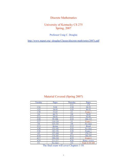
<strong>Discrete</strong> <strong>Mathematics</strong><br />
<strong>University</strong> <strong>of</strong> <strong>Kentucky</strong> <strong>CS</strong> <strong>275</strong><br />
<strong>Spring</strong>, 2007<br />
Pr<strong>of</strong>essor Craig C. Douglas<br />
http://www.mgnet.org/~douglas/Classes/discrete-math/notes/2007s.pdf<br />
Material Covered (<strong>Spring</strong> 2007)<br />
Tuesday Pages Thursday Pages<br />
1/11 1-9<br />
1/16 9-24 1/18 24-33<br />
1/23 34-45 1/25 46-52<br />
1/30 53-65 2/1 Exam 1<br />
2/6 66-73 2/8 74-83<br />
2/13 84-92 2/15 92-94<br />
2/20 95-106 2/22 106-115<br />
2/27 116-124 3/1 Exam 2<br />
3/6 125-132 3/8 No class<br />
3/13 <strong>Spring</strong> 3/15 Break<br />
3/20 132-142 3/22 No class<br />
3/26 142-156 3/28 Exam 3<br />
4/3 157-169 4/5 170-177<br />
4/10 178-185 4/12 186-197<br />
4/17 198-210 4/19 Exam 4<br />
4/24 211-217 4/26 Rama: review<br />
5/1 No class 5/3 Final: 8-10 AM<br />
The final exam will cover Chapters 1-10.<br />
2
Course Outline<br />
1. Logic Principles<br />
2. Sets, Functions, Sequences, and Sums<br />
3. Algorithms, Integers, and Matrices<br />
4. Induction and Recursion<br />
5. Simple Counting Principles<br />
6. <strong>Discrete</strong> Probability<br />
7. Advanced Counting Principles<br />
8. Relations<br />
9. Graphs<br />
10. Trees<br />
11. Boolean Algebra<br />
12. Modeling Computation<br />
3<br />
Logic Principles<br />
Basic values: T or F representing true or false, respectively. In a computer T an<br />
F may be represented by 1 or 0 bits.<br />
Basic items:<br />
• Propositions<br />
o Logic and Equivalences<br />
• Truth tables<br />
• Predicates<br />
• Quantifiers<br />
• Rules <strong>of</strong> Inference<br />
• Pro<strong>of</strong>s<br />
o Concrete, outlines, hand waving, and false<br />
4
Definition: A proposition is a statement <strong>of</strong> a true or false fact (but not both).<br />
Examples:<br />
• 2+2 = 4 is a proposition because this is a fact.<br />
• x+1 = 2 is not a proposition unless a specific value <strong>of</strong> x is stated.<br />
Definition: The negation <strong>of</strong> a proposition p, denoted by ¬p and pronounced not<br />
p, means that, “it is not the case that p.” The truth values for ¬p are the opposite<br />
for p.<br />
Examples:<br />
• p: Today is Thursay, ¬p: Today is not Thursday.<br />
• p: At least a foot <strong>of</strong> snow falls in Boulder on Fridays. ¬p: Less than a foot<br />
<strong>of</strong> snow falls in Boulder on Fridays.<br />
5<br />
Definition: The conjunction <strong>of</strong> propositions p and q, denoted p!q, is true if<br />
both p and q are true, otherwise false.<br />
Definition: The disjunction <strong>of</strong> propositions p and q, denoted p"q, is true if<br />
either p or q is true, otherwise false.<br />
Definition: The exclusive or <strong>of</strong> propositions p and q, denoted p#q, is true if<br />
only one <strong>of</strong> p and q is true, otherwise false.<br />
Truth tables:<br />
p ¬p q p!q p"q p#q<br />
T F T T T F<br />
T * F * F F T T<br />
F * T * T F T T<br />
F T F F F F<br />
* The truth table for p and ¬p is really a 2$2 table.<br />
6
Concepts so far can be extended to Boolean variables and Bit strings.<br />
Definition: A bit is a binary digit. Hence, it has two possible values: 0 and 1.<br />
Definition: A bit string is a sequence <strong>of</strong> zero or more bits. The length <strong>of</strong> a bit<br />
string is the number <strong>of</strong> bits.<br />
Definition: The bitwise operators OR, AND, and XOR are defined based on<br />
!, ", and #, bit by bit in a bit string.<br />
Examples:<br />
• 010111 is a bit string <strong>of</strong> length 6<br />
• 010111 OR 110000 = 110111<br />
• 010111 AND 110000 = 010000<br />
• 010111 XOR 110000 = 100111<br />
7<br />
Definition: The conditional statement is an implication, denoted p%q, and is<br />
false when p is true and q is false, otherwise it is true. In this case p is known<br />
as a hypothesis (or antecedent or premise) and q is known as the conclusion<br />
(or consequence).<br />
Definition: The biconditional statement is a bi-implication, denoted p&q, and<br />
is true if and only if p and q have the same truth table values.<br />
Truth tables:<br />
p q p%q p&q<br />
T T T T<br />
T F F F<br />
F T T F<br />
F F T T<br />
8
We can compound logical operators to make complicated propositions. In<br />
general, using parentheses makes the expressions clearer, even though more<br />
symbols are used. However, there is a well defined operator precedence<br />
accepted in the field. Lower numbered operators take precedence over higher<br />
numbered operators.<br />
Examples:<br />
• ¬p!q = (¬p) !q<br />
• p!q"r = (p!q) "r<br />
Operator Precedence<br />
¬ 1<br />
! 2<br />
" 3<br />
% 4<br />
& 5<br />
9<br />
Definition: A compound proposition that is always true is a tautology. One that<br />
is always false is a contradiction. One that is neither is a contingency.<br />
Example:<br />
p ¬p p!¬p p"¬p<br />
T F F T<br />
F T F T<br />
contigencies contradiction tautology<br />
Definition: Compound propositions p and q are logically equivalent if p&q is a<br />
tautology and is denoted p'q (sometimes written as p!q instead).<br />
10
Theorem: ¬(p"q) ' ¬p ! ¬q.<br />
Pro<strong>of</strong>: Construct a truth table.<br />
p q ¬(p"q) ¬p ¬q ¬p!¬q<br />
T T F F F F<br />
T F F F T F<br />
F T F T F F<br />
F F T T T T<br />
qed<br />
Theorem: ¬(p!q) ' ¬p " ¬q.<br />
Pro<strong>of</strong>: Construct a truth table similar to the previous theorem.<br />
These two theorems are known as DeMorgan’s laws and can be extended to any<br />
number <strong>of</strong> propositions:<br />
¬(p 1 "p 2 "…"p k ) ' ¬ p 1 ! ¬ p 2 ! … ! ¬ p k<br />
¬(p 1 !p 2 !…!p k ) ' ¬ p 1 " ¬ p 2 " … " ¬ p k<br />
11<br />
Theorem: p%q ' ¬p"q.<br />
Pro<strong>of</strong>: Construct a truth table.<br />
p q p%q ¬p ¬p"q<br />
T T T F T<br />
T F F F F<br />
F T T T T<br />
F F T T T<br />
qed<br />
These pro<strong>of</strong>s are examples are concrete ones that are proven using an exhaustive<br />
search <strong>of</strong> all possibilities. As the number <strong>of</strong> propositions grows, the number <strong>of</strong><br />
possibilities grows like 2 k for k propositions.<br />
The distributive laws are an example when k=3.<br />
12
Theorem: p" (q!r) ' (p"q)!(p"r).<br />
Pro<strong>of</strong>: Construct a truth table.<br />
p q r p" (q!r) p"q p"r (p"q)!(p"r)<br />
T T T T T T T<br />
T T F T T T T<br />
T F T T T T T<br />
T F F T T T T<br />
F T T T T T T<br />
F T F F T F F<br />
F F T F F T F<br />
F F F F F F F<br />
qed<br />
Theorem: p! (q"r) ' (p!q) " (p!r).<br />
Pro<strong>of</strong>: Construct a truth table similar to the previous theorem.<br />
13<br />
Some well known logical equivalences includes the following laws:<br />
'<br />
p!T'p<br />
p"F'p<br />
p"T'T<br />
p!F'F<br />
p"p'p<br />
p!p'p<br />
¬(¬p) 'p<br />
p"¬p 'T<br />
p!¬p 'F<br />
p"q'q"p<br />
p!q'q!p<br />
(p"q)"r' p"(q"r)<br />
(p!q) !r' p!(q!r)<br />
Law<br />
Identity<br />
Domination<br />
Idempotent<br />
Double negation<br />
Negation<br />
Commutative<br />
Associative<br />
14
'<br />
p"(q!r) '(p"q)!(q"r)<br />
p!(q"r) '(p!q)"(q!r)<br />
¬(p"q) ' ¬p!¬q<br />
¬(p!q) ' ¬p"¬q<br />
p"(p!q)'p<br />
p!(p"q)'p<br />
Law<br />
Distributive<br />
DeMorgan<br />
Absorption<br />
All <strong>of</strong> these laws can be proven concretely using truth tables. It is a good<br />
exercise to see if you can prove some.<br />
15<br />
Well known logical equivalences involving conditional statements:<br />
p%q ' ¬p"q<br />
p%q ' ¬q%¬p<br />
p"q ' ¬p%q<br />
p!q ' ¬(p%¬q)<br />
¬(p%q) ' p!¬q<br />
(p%q)!(p%r) ' p%(q!r)<br />
(p%r)!(q%r) ' (p"q)%r<br />
(p%q)"(p%r) ' p%(q"r)<br />
(p%r)"(q%r) ' (p!q)%r<br />
Well known logical equivalences involving biconditional statements:<br />
p&q ' (p%q)!(q%p)<br />
p&q ' ¬p&¬q<br />
p&q ' (p!q) " (¬p!¬q)<br />
¬(p&q) ' p&¬q<br />
16
Propositional logic is pretty limited. Almost anything you really are interested in<br />
requires a more sophisticated form <strong>of</strong> logic: predicate logic with quantifiers (or<br />
predicate calculus).<br />
Definition: P(x) is a propositional function when a specific value x is substituted<br />
for the expression in P(x) gives us a proposition. The part <strong>of</strong> the expression<br />
referring to x is known as the predicate.<br />
Examples:<br />
• P(x): x > 24. P(2) = F, P(102) = T.<br />
• P(x): x = y + 1. P(x) = T for one value only (y is an unbounded variable).<br />
• P(x,y): x = y + 1. P(2,1) = T, P(102,-14) = F.<br />
Definition: A statement <strong>of</strong> the form P(x 1 ,x 2 ,…,x n ) is the value <strong>of</strong> the<br />
propositional function P at the n-tuple (x 1 ,x 2 ,…,x n ). P is also known as a n-place<br />
(or n-ary) predicate.<br />
17<br />
Definition: The universal quantification <strong>of</strong> P(x) is the statement P(x) is true for<br />
all values <strong>of</strong> x in some domain, denoted by (x P(x).<br />
Definition: The existential quantification <strong>of</strong> P(x) is the statement P(x) is true for<br />
at least one value <strong>of</strong> x in some domain, denoted by )x P(x).<br />
Definition: The uniqueness quantification <strong>of</strong> P(x) is the statement P(x) is true for<br />
exactly one value <strong>of</strong> x in some domain, denoted by )!x P(x).<br />
There is an infinite number <strong>of</strong> quantifiers that can be constructed, but the three<br />
above are among the most important and common.<br />
Examples: Assume x belongs to the real numbers.<br />
• (x 0). The negative real numbers form the domain.<br />
• )!x (x 1223 = 0).<br />
18
( and ) have higher precedence than the logical operators.<br />
Example: (x P(x)!Q(x) means ((x P(x))!Q(x).<br />
Definition: When a variable is used in a quantification, it is said to be bound.<br />
Otherwise the variable is free.<br />
Example: )x (x = y + 1).<br />
Definition: Statements involving predicates and quantifiers are logically<br />
equivalent if and only if they have the same truth value independent <strong>of</strong> which<br />
predicates are substituted and in which domains are used. Notation: S ' T.<br />
DeMorgan’s Laws for Negation:<br />
• ¬)x P(x) ' (x ¬P(x).<br />
• ¬(x P(x) ' )x ¬P(x).<br />
19<br />
Nested quantifiers just means that more than one is in a statement. The order <strong>of</strong><br />
quantifiers is important.<br />
Examples: Assume x and y belong to the real numbers.<br />
• (x)y (x + y = 0).<br />
• (x(y (x < 0) ! (y > 0) % xy < 0.<br />
Quantification <strong>of</strong> two variables:<br />
Statement When True? When False?<br />
(x(y P(x,y) For all x and y, P(x,y)=T. There is a pair <strong>of</strong> x and y such that<br />
P(x,y)=F.<br />
(x)y P(x,y) For all x there is a y such There is an x such that for all y,<br />
that P(x,y)=T<br />
P(x,y)=F.<br />
)x(y P(x,y) There is an x such that for For all x there is a y such that<br />
)x)y P(x,y)<br />
all y, P(x,y)=T.<br />
There is a pair x and y<br />
such that P(x,y)=T.<br />
P(x,y)=F.<br />
For all x and y, P(x,y)=F.<br />
20
Rules <strong>of</strong> Inference are used instead <strong>of</strong> truth tables in many instances. For n<br />
variables, there are 2 n rows in a truth table, which gets out <strong>of</strong> hand quickly.<br />
Definition: A propositional logic argument is a sequence <strong>of</strong> propositions. The<br />
last proposition is the conclusion. The earlier ones are the premises. An<br />
argument is valid if the truth <strong>of</strong> the premises implies the truth <strong>of</strong> the conclusion.<br />
Definition: A propositional logic argument form is a sequence <strong>of</strong> compound<br />
propositions involving propositional variables. An argument form is valid if no<br />
matter what particular propositions are substituted for the proposition variables<br />
in its premises, the conclusion remains true if the premises are all true.<br />
Translation: An argument form with premises p 1 , p 2 , …, p n and conclusion q is<br />
valid when (p 1 !p 2 !…!p n ) % q is a tautology.<br />
21<br />
There are eight basic rules <strong>of</strong> inference.<br />
Rule Tautology Name<br />
p<br />
[p!( p%q)] % q Modus ponens<br />
p%q<br />
*q<br />
¬q<br />
[¬q!(p%q)] % ¬p Modus tollens<br />
p%q<br />
*¬p<br />
p%q<br />
[(p%q)!(q%r)] % (p%r) Hypothetical syllogism<br />
q%r<br />
* p%r<br />
p"q<br />
[(p"q)!¬p] % q Disjunctive syllogism<br />
¬p<br />
*q<br />
p<br />
*p"q<br />
p % (p"q)<br />
Addition<br />
22
Rule Tautology Name<br />
p!q<br />
(p!q) % p<br />
Simplification<br />
*p<br />
p<br />
[(p)!(q)] % (p!q) Conjunction<br />
q<br />
*p!q<br />
p"q<br />
¬p"r<br />
*q"r<br />
[(p"q)!(¬p"r)]% (q"r) Resolution<br />
23<br />
Rules <strong>of</strong> Inference for Quantified Statements:<br />
Rule <strong>of</strong> Inference<br />
(x P(x)<br />
*P(c)<br />
P(c) for an arbitrary c<br />
*(x P(x)<br />
(x (P(x) % Q(x))<br />
P(a), where a is a particular element in the domain<br />
*Q(a)<br />
(x (P(x) % Q(x))<br />
¬Q(a), where a is a particular element in the domain<br />
*¬P(a)<br />
)x P(x)<br />
*P(c) for some c<br />
P(c) for some c<br />
*)x P(x)<br />
Name<br />
Universal instantiation<br />
Universal generalization<br />
Universal modus ponens<br />
Universal modus tollens<br />
Existential instantiation<br />
Existential generalization<br />
24
Sets, Functions, Sequences, and Sums<br />
Definition: A set is a collection <strong>of</strong> unordered elements.<br />
Examples:<br />
• Z = {…, -3, -2, -1, 0, 1, 2, 3, …}<br />
• N = {1, 2, 3, …} and + = N 0 = {0, 1, 2, 3, …} (Slightly different than text)<br />
• Q = {p/q | p,q,Z, q-0}<br />
• R = {reals}<br />
Definition: The cardinality <strong>of</strong> a set S is denoted |S|. If |S| = n, where n,Z, then<br />
the set S is a finite set. Otherwise it is an infinite set (|S| = .).<br />
Example: The cardinality <strong>of</strong> <strong>of</strong> Z, N, N 0 , Q, and R is infinite.<br />
25<br />
Definition: If |S| = |N|, then S is a countable set. Otherwise it is an uncountable<br />
set.<br />
Examples:<br />
• Q is countable.<br />
• R is uncountable.<br />
Definition: Two sets S and T are equal, denoted S = T, if and only if (x(x,S &<br />
x,T).<br />
Examples:<br />
• Let S = {0, 1, 2} and T = {2, 0, 1}. Then S = T. Order does not count.<br />
• Let S = {0, 1, 2} and T = {0, 1, 3}. Then S - T. Only the elements count.<br />
Definition: The empty set is denoted by /. Note that (S(/,S).<br />
26
Definition: A set S is a subset <strong>of</strong> a set T if (x,S(x,T) and is denoted S0T. S is<br />
a proper subset <strong>of</strong> T if S0T, but S-T and is denoted S1T.<br />
Example: S = {1, 0} and T = {0, 1, 2}. Then S1T.<br />
Theorem: (S(S0S).<br />
Pro<strong>of</strong>: By definition, (x,S(x,S).<br />
27<br />
Definition: The Power Set <strong>of</strong> a set S, denoted P(S), is the set <strong>of</strong> all possible<br />
subsets <strong>of</strong> S.<br />
Theorem: If |S| = n, then |P(S)| = 2 n .<br />
Example: S = {0, 1}. Then P(S) = {/, {0}, {1}, {0,1}}<br />
Definition: The Cartesian product <strong>of</strong> n sets A i is defined by ordered elements<br />
from the A i and is denoted A 1 $A 2 $…$A n = {(a 1 ,a 2 ,…a n ) | a i ,A i }.<br />
Example: Let S = {0, 1} and T = {a, b}. Then S$T = {(0,a), (0,b), (1,a), (1,b)}.<br />
Definition: The union <strong>of</strong> n sets A i is defined by<br />
n<br />
! = A 1 2A 2 2…2A n = {x | )i x,A i }.<br />
i=1 A i<br />
Definition: The intersection <strong>of</strong> n sets A i is defined by<br />
n<br />
! = A 1 3A 2 3…3A n = {x | (i x,A i<br />
i=1 A i<br />
28
Definition: n sets A i are disjoint if A 1 3A 2 3…3A n = /.<br />
Definition: The complement <strong>of</strong> set S with respect to T, denoted T4S, is defined<br />
by T4S = {x,T | x6S}. T4S is also called the difference <strong>of</strong> S and T.<br />
Definitions: The universal set is denoted U. The universal complement <strong>of</strong> S is<br />
S = U4S.<br />
29<br />
Examples:<br />
• Let S = {1, 0} and T = {0, 1, 2}. Then<br />
o S1T.<br />
o S3T = S.<br />
o S2T = T.<br />
o T4S = {2}.<br />
o Let U = N 0 . S = {2, 3, …}<br />
• Let S = {0, 1} and T = {2, 3}. Then<br />
o S5T.<br />
o S3T = /.<br />
o S2T = {0, 1, 2, 3}.<br />
o T4S = {2, 3}.<br />
o Let U=R. Then S is the set <strong>of</strong> all reals except the integers 0 and 1, i.e.,<br />
S = {x,R | x-0 ! x-1}.<br />
30
The textbook has a large number <strong>of</strong> set identities in a table.<br />
Identity<br />
Law(s)<br />
A2/ = A, A3U = A Identity<br />
A2U = U, A3/ = /<br />
Domination<br />
A2A = A, A3A = A<br />
Idempotent<br />
A = A<br />
Complementation<br />
A2B = B2A, A3B = B3A<br />
Commutative<br />
A2(B2C) = (A2B)2C, A3 (B3C) = (A3B) 3C Associative<br />
A3 (B2C) = (A3B) 2 (A3C)<br />
Distributive<br />
A2(B3C) = (A2B) 3 (A2C)<br />
A!B = A"B, A!B = A"B<br />
DeMorgan<br />
A2 (A3B) = A, A3 (A2B) = A<br />
Absorption<br />
A!A = U, A"A = #<br />
Complement<br />
Many <strong>of</strong> these are simple to prove from very basic laws.<br />
31<br />
Definition: A function f:A%B maps a set A to a set B, denoted f(a) = b for a,A<br />
and b,B, where the mapping (or transformation) is unique.<br />
Definition: If f:A%B, then<br />
• If (b,B )a,A (f(a) = b), then f is a surjective function or onto.<br />
• If A=B and f(a) = f(b) implies a = b, then f is one-to-one (1-1) or injective.<br />
• A function f is a bijection or a one-to-one correspondence if it is 1-1 and<br />
onto.<br />
Definition: Let f:A%B. A is the domain <strong>of</strong> f. The minimal set B such that<br />
f:A%B is onto is the image <strong>of</strong> f.<br />
Definitions: Some compound functions include<br />
n<br />
n<br />
• (!<br />
f<br />
i i )(a) = ! f (a) i=1 i . We can substitute + if we expand the summation.<br />
n<br />
n<br />
• (!<br />
f<br />
i=1 i )(a)=! f (a) i=1 i . We can substitute * if we expand the product.<br />
32
Definition: The composition <strong>of</strong> n functions f i : A i %A i+1 is defined by<br />
(f 1 °f 2 °…°f n )(a) = f 1 (f 2 (…(f n (a)…)),<br />
where a,A 1 .<br />
Definition: If f: A%B, then the inverse <strong>of</strong> f, denoted f -1 : B%A exists if and only<br />
if (b,B )a,A (f(a) = b ! f -1 (b) = a).<br />
Examples:<br />
• Let A = [0,1] 1 R, B = [0,2] 1 R.<br />
o f(a) = a 2 and g(a) = a+1. Then f+g: A%B and f*g: A%B.<br />
o f(a) = 2*a and g(a) = a-1. Then neither f+g: A%B nor f*g: A%B.<br />
• Let B = A = [0,1] 1 R.<br />
o f(a) = a 2 and g(a) = 1-a. Then f+g: A%A and f*g: A%A. Both<br />
compound functions are bijections.<br />
o f(a) = a 3 and g(a) = a 1/3 . Then g°f(a): A%A is a bijection.<br />
• Let A = [-1, 1] and B=[0, 1]. Then<br />
o f(a) = a 3 and g(a) = {x>0 | x= a 1/3 }. Then g°f(a): A%B is onto.<br />
33<br />
Definition: The graph <strong>of</strong> a function f is {(a,f(a)) | a,A}.<br />
Example: A = {0, 1, 2, 3, 4, 5} and f(a) = a 2 . Then<br />
(a) graph(f,A)<br />
(b) an approximation to graph(f,[0,5])<br />
34
Definitions: The floor and ceiling functions are defined by<br />
Examples:<br />
• 7x8 = largest integer smaller or equal to x.<br />
• 9x: = smallest integer larger or equal to x.<br />
• 72.998 = 2, 92.99: = 3<br />
• 7-2.998 = -3, 9-2.99: = -2<br />
Definition: A sequence is a function from either N or a subset <strong>of</strong> N to a set A<br />
whose elements a i are the terms <strong>of</strong> the sequence.<br />
Definitions: A geometric progression is a sequence <strong>of</strong> the form {ar i , i=0, 1, …}.<br />
An arithmetic progression is a sequence <strong>of</strong> the form {a+id, i=0, 1,…}.<br />
Translation: f(a,r,i) = ar i and f(a,d,i) = a + id are the corresponding functions.<br />
35<br />
There are a number <strong>of</strong> interesting summations that have closed form solutions.<br />
Theorem: If a,r,R, then<br />
"(n+1)a,<br />
if r=1,<br />
n $<br />
! ar i =<br />
i=0<br />
# ar n+1 -a<br />
$<br />
% r-1 , otherwise.<br />
Pro<strong>of</strong>: If r = 1, then we are left summing a n+1 times. Hence, the r = 1 case is<br />
n<br />
trivial. Suppose r - 1. Let S = ! ar i . Then<br />
n<br />
i=0<br />
i=0<br />
rS = r! ar i<br />
Substitution S formula.<br />
n+1<br />
! ar i<br />
Simplifying.<br />
"<br />
#<br />
$<br />
!<br />
i=1<br />
n<br />
i=0<br />
ar i<br />
S+(ar n+1 -a)<br />
( ) Removing n+1 term and adding 0 term.<br />
%<br />
&<br />
' + arn+1 -a<br />
Substituting S for formula<br />
Solve for S in rS = S+(ar n+1 -a) to get the desired formula.<br />
qed<br />
36
Some other common summations with closed form solutions are<br />
Sum<br />
Closed Form Solution<br />
n<br />
i<br />
n(n+1)<br />
! i=1<br />
2<br />
n<br />
! i<br />
i=1<br />
2<br />
n(n+1)(2n+1)<br />
6<br />
n<br />
! i<br />
i=1<br />
3<br />
n 2 (n+1) 2<br />
4<br />
!<br />
! x<br />
i=0<br />
i , |x|
Theorem: If f i (x) is O(g i (x)), for 1;i;n, then<br />
n<br />
i=1<br />
! f i<br />
(x) is O(max{|g 1 (x)|, |g 2 (x)|, …, |g n (x)|}).<br />
Pro<strong>of</strong>: Let g(x) = max{|g 1 (x)|, |g 2 (x)|, …, |g n (x)|} and C i the constants associated<br />
with O(g i (x)). Then<br />
n<br />
i=1<br />
n<br />
i=1<br />
n<br />
i=1<br />
! f i<br />
(x) ; ! C i<br />
g i<br />
(x) ; ! C i<br />
g(x) = |g(x)| ! C i<br />
= C|g(x)|.<br />
Theorem: If f i (x) is O(g i (x)), for 1;i;n, then ! f i<br />
(x) is O( ! g i<br />
(x) ).<br />
Pro<strong>of</strong>: Let g(x) = |g 1 (x)|$|g 2 (x)|$…|g n (x)| and C i the constants associated with<br />
O(g i (x)). Then<br />
n<br />
i=1<br />
n<br />
i=1<br />
n<br />
i=1<br />
! f i<br />
(x) ; ! C i<br />
g i<br />
(x) ; C! g i<br />
(x) .<br />
n<br />
i=1<br />
n<br />
i=1<br />
n<br />
i=1<br />
39<br />
Definition: Let f and g be functions from either Z or R to R. Then f(x) is<br />
=(g(x)) if there are constants C and k such that |f(x)| < C|g(x)| whenever x>k.<br />
Definition: Let f and g be functions from either Z or R to R. Then f(x) is<br />
>(g(x)) if f(x) = O(g(x)) and f(x) = =(g(x)). In this case, we say that f(x) is <strong>of</strong><br />
order g(x).<br />
Comment: f(x) = O(g(x)) notation is great in the limit, but does not always<br />
provide the right bounds for all values <strong>of</strong> x. =, denoted Big Omega, is used to<br />
provide lower bounds. >, denoted Big Theta, is used to provide both lower and<br />
upper bounds.<br />
n<br />
i=0<br />
Example: f(x) = ! a i<br />
x i with a n -0 is <strong>of</strong> order x n .<br />
40
Notation: Timing, as a function <strong>of</strong> the number <strong>of</strong> elements falls into the field <strong>of</strong><br />
Complexity.<br />
Complexity Terminology<br />
>(1) Constant<br />
>(log(n)) Logarithmic<br />
>(n)<br />
Linear<br />
>(nlog(n)) nlog(n)<br />
>(n k )<br />
Polynomial<br />
>(n k log(n)) Polylog<br />
>(k n ), where k>1 Exponential<br />
>(n!)<br />
Factorial<br />
Notation: Problems are tractable if they can be solved in polynomial time and<br />
are intractable otherwise.<br />
41<br />
Algorithms, Integers, and Matrices<br />
Definition: An algorithm is a finite set <strong>of</strong> precise instructions for solving a<br />
problem.<br />
Computational algorithms should have these properties:<br />
• Input: Values from a specified set.<br />
• Output: Results using the input from a specified set.<br />
• Definiteness: The steps in the algorithm are precise.<br />
• Correctness: The output produced from the input is the right solution.<br />
• Finiteness: The results are produced using a finite number <strong>of</strong> steps.<br />
• Effectiveness: Each step must be performable and in a finite amount <strong>of</strong><br />
time.<br />
• Generality: The procedure should accept all input from the input set, not<br />
just special cases.<br />
42
!<br />
Algorithm: Find the maximum value <strong>of</strong> " a i<br />
! $<br />
procedure max( " a<br />
# i<br />
% : integers)<br />
&i=1<br />
max := a 1<br />
for i := 2 to n<br />
if max < a i then max := a i<br />
{max is the largest element}<br />
n<br />
#<br />
n<br />
$<br />
%<br />
&i=1<br />
, where n is finite.<br />
Pro<strong>of</strong> <strong>of</strong> correctness: We use induction.<br />
1. Suppose n = 1, then max := a 1 , which is the correct result.<br />
2. Suppose the result is true for k = 1, 2, …, i-1. Then at step i, we know that<br />
max is the largest element in a 1 , a 2 , …, a i-1 . In the if statement, either max is<br />
already larger than a i or it is set to a i . Hence, max is the largest element in<br />
a 1 , a 2 , …, a i . Since i was arbitrary, we are done. qed<br />
This algorithm’s input and output are well defined and the overall algorithm can<br />
be performed in O(n) time since n is finite. There are no restrictions on the input<br />
set other than the elements are integers.<br />
43<br />
!<br />
Algorithm: Find a value in a sorted, distinct valued " a<br />
# i<br />
There are many, many search algorithms.<br />
! $<br />
procedure linear_search(x, " a<br />
# i<br />
% : integers)<br />
&i=1<br />
i := 1<br />
while (i;n and x-a i )<br />
i := i + 1<br />
if i;n then location := i else location := 0<br />
!<br />
{location is the subscript <strong>of</strong> " a<br />
# i<br />
n<br />
n<br />
$<br />
%<br />
&i=1<br />
n<br />
$<br />
%<br />
&i=1<br />
, where n is finite.<br />
!<br />
equal to x or 0 if x is not in " a<br />
# i<br />
n<br />
$<br />
% }<br />
&i=1<br />
We can prove that this algorithm is correct using an induction argument. This<br />
algorithm does not rely on either distinctiveness nor sorted elements.<br />
Linear search works, but it is very slow in comparison to many other searching<br />
algorithms. It takes 2n+2 comparisons in the worst case, i.e., O(n) time.<br />
44
! $<br />
procedure binary_search(x, " a<br />
# i<br />
% : integers)<br />
&i=1<br />
i := 1<br />
j := n<br />
while ( i < j )<br />
m := 7(i+j)/28<br />
if x > a m then i := m+1 else j := m<br />
if x = a i then location := i else location := 0<br />
!<br />
{location is the subscript <strong>of</strong> " a<br />
# i<br />
n<br />
n<br />
$<br />
%<br />
&i=1<br />
!<br />
equal to x or 0 if x is not in " a<br />
# i<br />
We can prove that this algorithm is correct using an induction argument.<br />
n<br />
$<br />
% }<br />
&i=1<br />
This algorithm is much, much faster than linear_search on average. It is O(logn)<br />
!<br />
in time. The average time to find a member <strong>of</strong> " a<br />
# i<br />
order n.<br />
n<br />
$<br />
%<br />
&i=1<br />
can be proven to be <strong>of</strong><br />
45<br />
!<br />
Algorithm: Sort the distinct valued " a<br />
# i<br />
finite.<br />
n<br />
$<br />
%<br />
&i=1<br />
into increasing order, where n is<br />
There are many, many sorting algorithms.<br />
! $<br />
procedure bubble_sort( " a<br />
# i<br />
% : reals, n>1)<br />
&i=1<br />
for i := 1 to n-1<br />
for j := 1 to n-i<br />
if a j > a j+1 then swap a j and a j+1<br />
!<br />
{ " a<br />
# i<br />
n<br />
$<br />
%<br />
&i=1<br />
is in increasing order}<br />
n<br />
This is one <strong>of</strong> the simplest sorting algorithms. It is expensive, however, but quite<br />
easy to understand and implement. Only one temporary is needed for the<br />
swapping and two loop variables as extra storage. The worst case time is O(n 2 ).<br />
46
!<br />
procedure insertion_sort( " a<br />
# i<br />
for j := 2 to n<br />
i := 1<br />
while a j > a i<br />
i := i + 1<br />
t := a j<br />
for k := 0 to j-i-1<br />
a j-k := a j-k-1<br />
a i := t<br />
!<br />
{ " a<br />
# i<br />
n<br />
$<br />
%<br />
&i=1<br />
n<br />
$<br />
%<br />
&i=1<br />
is in increasing order}<br />
: reals, n>1)<br />
This is not a very efficient sorting algorithm either. However, it is easy to see<br />
that at the j th step that the j th element is put into the correct spot. The worst case<br />
time is O(n 2 ). In fact, insertion_sort is trivially slower than bubble_sort.<br />
47<br />
Number theory is a rich field <strong>of</strong> mathematics. We will study four aspects briefly:<br />
1. Integers and division<br />
2. Primes and greatest common denominators<br />
3. Integers and algorithms<br />
4. Applications <strong>of</strong> number theory<br />
Most <strong>of</strong> the theorems quoted in this part <strong>of</strong> the textbook require knowledge <strong>of</strong><br />
mathematical induction to rigorously prove, a topic covered in detail in the next<br />
chapter. !<br />
48
Definition: If a,b,Z and a-0, we say that a divides b if )c,Z(b=ac), denoted by<br />
a | b. When a divides b, we denote a as a factor <strong>of</strong> b and b as a multiple <strong>of</strong> a.<br />
When a does not divide b, we denote this as a/|b.<br />
Theorem: Let a,b,c,Z. Then<br />
1. If a | b and a | c, then a | (b+c).<br />
2. If a | b, then a | (bc).<br />
3. If a | b and b | c, then a | c.<br />
Pro<strong>of</strong>: Since a | b, )s,Z(b=as).<br />
1. Since a | c it follows that ) t,Z(c=at). Hence, b+c = as + at = a(s+t).<br />
Therefore, a | (b+c).<br />
2. bc = (as)c = a(sc). Therefore, a | (bc).<br />
3. Since b | c it follows that ) t,Z(c=bt). c = bt = (as)t = a(st), Therefore, a | c.<br />
Corollary: Let a,b,c,Z. If a | b and b | c, then a | (mb+nc) for all m,n,Z.<br />
49<br />
Theorem (Division Algorithm): Let a,d,Z(d > 0). Then )!q,r,Z(a = dq+r).<br />
Definition: In the division algorithm, a is the dividend, d is the divisor, q is the<br />
quotient, and r is the remainder. We write q = a div d and r = a mod d.<br />
Examples:<br />
• Consider 101 divided by 9: 101 = 11$9 + 2.<br />
• Consider -11 divided by 3: -11 = 3(-4) + 1.<br />
Definition: Let a,b,m,Z(m > 0). Then a is congruent to b modulo m if m | (a-b),<br />
denoted a ' b (mod m). The set <strong>of</strong> integers congruent to an integer a modulo m<br />
is called the congruence class <strong>of</strong> a modulo m.<br />
Theorem: Let a,b,m,Z(m > 0). Then a ' b (mod m) if and only if a mod m = b<br />
mod m.<br />
50
Examples:<br />
• Does 17 ' 5 mod 6? Yes, since 17 – 5 = 12 and 6 | 12.<br />
• Does 24 ' 14 mod 6? No, since 24 – 14 = 10, which is not divisible by 6.<br />
Theorem: Let a,b,m,Z(m > 0). Then a ' b (mod m) if and only if<br />
)k,Z(a=b+km).<br />
Pro<strong>of</strong>: If a ' b (mod m), then m | (a-b). So, there is a k such that a-b = km, or a =<br />
b+km. Conversely, if there is a k such that a = b + km, then km = a-b. Hence, m<br />
| (a-b), or a ' b (mod m).<br />
Theorem: Let a,b,c,d,m,Z(m > 0). If a ' b (mod m) and c ' d (mod m), then<br />
a+c ' b+d (mod m) and ac ' bd (mod m).<br />
Corollary: Let a,b,m,Z(m > 0). Then (a+b) mod m = ((a mod m)+(b mod m))<br />
mod m and (ab) mod m = ((a mod m)(b mod m)) mod m.<br />
51<br />
Some applications involving congruence include<br />
• Hashing functions h(k) = k mod m.<br />
• Pseudorandom numbers: x n+1 = (ax n +c) mod m.<br />
o c = 0 is known as a pure multiplicative generator.<br />
o c - 0 is known as a linear congruential generator.<br />
• Cryptography<br />
Definition: A positive integer a is a prime if it is divisible only by 1 and a. It is a<br />
composite otherwise.<br />
Fundamental Theorem <strong>of</strong> Arithmetic: Every positive integer greater than 1 can<br />
be written uniquely as a prime or the product <strong>of</strong> two or more primes where the<br />
prime factors are written in nondecreasing order.<br />
Theorem: If a is a composite number, then a has a prime divisor less than or<br />
equal to a 1/2 .<br />
52
Theorem: There are infinitely many primes.<br />
Prime Number Theorem: The ratio <strong>of</strong> primes not exceeding a and x/ln(a)<br />
approaches 1 as a%..<br />
Example: The odds <strong>of</strong> a randomly chosen positive integer n being prime is given<br />
by (n/ln(n))/n = 1/ln(n) asymptotically.<br />
There are still a number <strong>of</strong> open questions regarding the distribution <strong>of</strong> primes.<br />
Definition: Let a,b,Z(a and b not both 0). The largest integer d such that d | a<br />
and d | b is the greatest common devisor <strong>of</strong> a and b, denoted by gcd(a,b).<br />
Example: gcd(24,36) = 12.<br />
Definition: The integers a and b are relatively prime if gcd(a,b) = 1.<br />
53<br />
!<br />
Definition: The integers " a<br />
# i<br />
whenever 1;i
Integers can be expressed uniquely in any base.<br />
Theorem: Let b,Z(b>1). Then if n,N, then there is a unique expression such<br />
that n = a k b k + a k-1 b k-1 +…+a 1 b+a 0 , where {a i },k,N 0 , a k -0, and 0;a i 1, is really easy. Just group k bits together and<br />
convert to the base 2 k symbol.<br />
• Base 10 to any base 2 k is a pain.<br />
• Base 2 k to base 10 is also a pain.<br />
56
Algorithm: Addition <strong>of</strong> integers<br />
procedure add(a, b: integers)<br />
(a n-1 a n-2 …a 1 a 0 ) 2 := base_2_expansion(a)<br />
(b n-1 b n-2 …b 1 b 0 ) 2 := base_2_expansion(b)<br />
c := 0<br />
for j := 0 to n-1<br />
d := 7(a j +b j +c)/28<br />
s j := a j +b j +c – 2d<br />
c := d<br />
s n := c<br />
{the binary expansion <strong>of</strong> the sum is (s k-1 s k-2 …s 1 s 0 ) 2 }<br />
Questions:<br />
• What is the complexity <strong>of</strong> this algorithm?<br />
• Is this the fastest way to compute the sum?<br />
57<br />
Algorithm: Mutiplication <strong>of</strong> integers<br />
procedure multiply(a, b: integers)<br />
(a n-1 a n-2 …a 1 a 0 ) 2 := base_2_expansion(a)<br />
(b n-1 b n-2 …b 1 b 0 ) 2 := base_2_expansion(b)<br />
for j := 0 to n-1<br />
if b j = 1 then c j := a shifted j places else c j := 0<br />
{c 0 ,c 1 ,…,c n-1 are the partial products}<br />
p := 0<br />
for j := 0 to n-1<br />
p := p + c j<br />
{p is the value <strong>of</strong> ab}<br />
Examples:<br />
• (10) 2 $(11) 2 = (110) 2 . Note that there are more bits than the original integers.<br />
• (11) 2 $(11) 2 = (1001) 2 . Twice as many binary digits!<br />
58
Algorithm: Compute div and mod<br />
procedure division(a: integer, d: positive integer)<br />
q := 0<br />
r := |a|<br />
while r < d<br />
r := r – d<br />
q := q + 1<br />
if a < 0 and r > 0 then<br />
r := d – r<br />
q := -(q + 1)<br />
{q = a div d is the quotient and r = a mod d is the remainder}<br />
Notes:<br />
• The complexity <strong>of</strong> the multiplication algorithm is O(n 2 ). Much more<br />
efficient algorithms exist, including one that is O(n 1.585 ) using a divide and<br />
conquer technique we will see later in the course.<br />
• There are O(log(a)log(d)) complexity algorithms for division.<br />
59<br />
Modular exponentiation, b k mod m, where b, k, and m are large integers is<br />
important to compute efficiently to the field <strong>of</strong> cryptology.<br />
Algorithm: Modular exponentiation<br />
procedure modular_exponentiation(b: integer, k,m: positive integers)<br />
(a n-1 a n-2 …a 1 a 0 ) 2 := base_2_expansion(k)<br />
y := 1<br />
power := b mod m<br />
for i := 0 to n-1<br />
if a i = 1 then y := (y $ power) mod m<br />
power := (power $ power) mod m<br />
{y = b k mod m}<br />
Note: The complexity is O((log(m)) 2 log(k)) bit operations, which is fast.<br />
60
Euclidean Algorithm: Compute gcd(a,b)<br />
procedure gcd(a,b: positive integers)<br />
x := a<br />
y := b<br />
while y-0<br />
r := x mod y<br />
x := y<br />
y := r<br />
{gcd(a,b) is x}<br />
Correctness <strong>of</strong> this algorithm is based on<br />
Lemma: Let a=bq+r, where a,b,q,r,Z. then gcd(a,b) = gcd(b,r).<br />
The complexity will be studied after we master mathematical induction.<br />
61<br />
Number theory useful results<br />
Theorem: If a,b,N then )s,t,Z(gcd(a,b) = sa+tb).<br />
Lemma: If a,b,c,N (gcd(a,b) = 1 and a | bc, then a | c).<br />
Note: This lemma makes proving the prime factorization theorem doable.<br />
Lemma: If p is a prime and p | a 1 a 2 …a n where each a i ,Z, then p | a i for some i.<br />
Theorem: Let m,N and let a,b,c,Z. If ac ' bc (mod m) and gcd(c,m) = 1, then<br />
a ' b (mod m).<br />
Definition: A linear congruence is a congruence <strong>of</strong> the form ax ' b (mod m),<br />
where m,N, a,b,Z, and x is a variable.<br />
Definition: An inverse <strong>of</strong> a modulo m is an a such that aa ' 1 (mod m).<br />
62
Theorem: If a and m are relatively prime integers and m>1, then an inverse <strong>of</strong> a<br />
modulo m exists and is unique modulo m.<br />
Pro<strong>of</strong>: Since gcd(a,m) = 1, )s,t,Z(1 = sa+tb). Hence, sa=tb ' 1 (mod m). Since<br />
tm ' 0 (mod m), it follows that sa ' 1 (mod m). Thus, s is the inverse <strong>of</strong> a<br />
modulo m. The uniqueness argument is made by assuming there are two<br />
inverses and proving this is a contradiction.<br />
Systems <strong>of</strong> linear congruences are used in large integer arithmetic. The basis for<br />
the arithmetic goes back to China 1700 years ago.<br />
Puzzle Sun Tzu (or Sun Zi): There are certain things whose number is unknown.<br />
• When divided by 3, the remainder is 2.<br />
• When divided by 5, the remainder is 3, and<br />
• When divided by 7, the remainder is 2.<br />
What will be the number <strong>of</strong> things? (Answer: 23… stay tuned why).<br />
63<br />
Chinese Remander Theorem: Let m 1 , m 2 ,…,m n ,N be pairwise relatively prime.<br />
n<br />
Then the system x ' a i (mod m i ) has a unique solution modulo m = ! .<br />
i=1<br />
m i<br />
Existence Pro<strong>of</strong>: The pro<strong>of</strong> is by construction. Let M k = m / m k , 1;k;n. Then<br />
gcd(M k , m k ) = 1 (from pairwise relatively prime condition). By the previous<br />
theorem we know that there is a y k which is an inverse <strong>of</strong> M k modulo m k , i.e.,<br />
M k y k ' 1 (mod m k ). To construct the solution, form the sum<br />
x = a 1 M 1 y 1 + a 2 M 2 y 2 + … + a n M n y n .<br />
Note that M j ' 0 (mod m k ) whenever j-k. Hence,<br />
x ' a k M k y k ' a k (mod m k ), 1;k;n.<br />
We have shown that x is simultaneous solution to the n congruences. qed<br />
64
Sun Tzu’s Puzzle: The a k ,{2, 1, 2} from 2 pages earlier. Next<br />
The inverses y k are<br />
m k ,{3, 5, 7}, m=3$5$7=105, and M k =m/m k ,{35, 21, 15}.<br />
1. y 1 = 2 (M 1 = 35 modulo 3).<br />
2. y 2 = 1 (M 2 = 21 modulo 5).<br />
3. y 3 = 1 (M 3 = 15 modulo 7).<br />
The solutions to this system are those x such that<br />
x ' a 1 M 1 y 1 + a 2 M 2 y 2 + a 2 M 2 y 2 = 2$35$2 + 3$21$1 + 2$15$1 = 233<br />
Finally, 233 ' 23 (mod 105).<br />
65<br />
Definition: A m$n matrix is a rectangular array <strong>of</strong> numbers with m rows and n<br />
columns. The elements <strong>of</strong> a matrix A are noted by A ij or a ij . A matrix with m=n<br />
is a square matrix. If two matrices A and B have the same number <strong>of</strong> rows and<br />
columns and all <strong>of</strong> the elements A ij = B ij , then A = B.<br />
Definition: The transpose <strong>of</strong> a m$n matrix A = [A ij ], denoted A T , is A T = [A ji ]. A<br />
matrix is symmetric if A = A T and skew symmetric if A = -A T .<br />
Definition: The i th row <strong>of</strong> an m$n matrix A is [A i1 , A i2 , …, A in ]. The j th column<br />
is [A 1j , A 2j , …, A mj ] T .<br />
Definition: Matrix arithmetic is not exactly the same as scalar arithmetic:<br />
• C = A + B: c ij = a ij + b ij , where A and B are m$n.<br />
• C = A – B: c ij = a ij - b ij , where A and B are m$n<br />
k<br />
• C = AB: c ij<br />
= ! a ip<br />
b pj<br />
, where A is m$k, B is k$n, and C is m$n.<br />
p=1<br />
66
Theorem: A±B = B±A, but AB-BA in general.<br />
Definition: The identity matrix I n is n$n with I ii = 1 and I ij = 0 if i-j.<br />
Theorem: If A is n$n, then AI n = I n A = A.<br />
Definition: A r = AA … A (r times).<br />
Definition: Zero-One matrices are matrices A = [a ij ] such that all a ij ,{0, 1}.<br />
Boolean operations are defined on m$n zero-one matrices A = [a ij ] and B = [b ij ]<br />
by<br />
• Meet <strong>of</strong> A and B: A!B = a ij !b ij , 1;i;m and 1;j;n.<br />
• Join <strong>of</strong> A and B: A"B = a ij "b ij , 1;i;m and 1;j;n.<br />
• The Boolean product <strong>of</strong> A and B is C = A !B, where A is m$k, B is k$n,<br />
and C is m$n, is defined by c ij = (a i1 !b 1j )"(a i2 !b 2j )"…"(a ik !b kj ).<br />
Definition: The Boolean power <strong>of</strong> a n$n matrix A is defined by A [r] =<br />
A !A !… !A (r times), where A [0] = I n .<br />
67<br />
Induction and Recursion<br />
Principle <strong>of</strong> Mathematical Induction: Given a propositional function P(n), n,N,<br />
we prove that P(n) is true for all n,N by verifying<br />
1. (Basis) P(1) is true<br />
2. (Induction) P(k)%P(k+1), (k,N.<br />
Notes:<br />
• Equivalent to [P(1) ! (k,N (P(k)%P(k+1))] % (n,N P(n).<br />
• We do not actually assume P(k) is true. It is shown that if it is assumed that<br />
P(k) is true, then P(k+1) is also true. This is a subtle grammatical point with<br />
mathematical implications.<br />
• Mathematical induction is a form <strong>of</strong> deductive reasoning, not inductive<br />
reasoning. The latter tries to make conclusions based on observations and<br />
rules that may lead to false conclusions.<br />
• Sometimes P(1) is not the basis, but some other P(k), k,Z.<br />
68
• Sometimes P(k) is for a (possibly infinite) subset <strong>of</strong> N or Z.<br />
• Sometimes P(k-1)%P(k) is easier to prove than P(k)%P(k+1).<br />
• Being flexible, but staying within the guiding principle usually works.<br />
• There are many ways <strong>of</strong> proving false results using subtly wrong induction<br />
arguments. Usually there is a disconnect between the basis and induction<br />
parts <strong>of</strong> the pro<strong>of</strong>.<br />
• Examples 10, 11, and 12 in your textbook are worth studying until you<br />
really understand each.<br />
n<br />
Lemma: ! (2i-1) = n<br />
i=1<br />
2 (sum <strong>of</strong> odd numbers).<br />
Pro<strong>of</strong>: (Basis) Take k = 1, so 1 = 1.<br />
(Induction) Assume 1+3+5+…+(2k-1) = k 2 for an arbitrary k > 1. Add 2k+1 to<br />
both sides. Then (1+3+5+…+(2k-1))+(2k+1) = k 2 +(2k+1) = (k+1) 2 .<br />
69<br />
n<br />
i=0<br />
Lemma: ! 2 i = 2 n+1 -1.<br />
Pro<strong>of</strong>: (Basis) Take k=0, so 2 0 = 1 = 2 1 – 1.<br />
k<br />
(Induction) Assume ! 2<br />
i=0<br />
i = 2 k+1 -1 for an arbitrary k > 0. Add 2 k+1 to both<br />
sides. Then<br />
k<br />
! 2<br />
i=0<br />
i + 2 k+1 = 2 k+1 -1 + 2 k+1 ,<br />
which simplifies to<br />
k+1<br />
2<br />
i=0<br />
i<br />
! = 2 k+2 -1.<br />
Principle <strong>of</strong> Strong Induction: Given a propositional function P(n), n,N, we<br />
prove that P(n) is true for all n,N by verifying<br />
1. (Basis) P(1) is true<br />
2. (Induction) [P(1)!P(2)!…!P(k)]%P(k+1) is true (k,N.<br />
70
Example: Infinite ladder with reachable rungs. For mathematical or strong<br />
induction, we need to verify the following:<br />
Step Mathematical Strong<br />
Basis<br />
We can reach the first rung.<br />
Induction If we can reach an arbitrary (k,N, if we can reach all k<br />
rung k, then we can reach rungs, then we can reach<br />
rung k+1.<br />
rung k+1.<br />
We cannot prove that you can climb an infinite ladder using mathematical<br />
induction. Using strong induction, however, you can prove this result using a<br />
trick: since you can prove that you can climb to rungs 1, 2, …, k, it follows that<br />
you can climb 2 rungs arbitrarily, which gets you from rung k-1 to rung k+1.<br />
Rule <strong>of</strong> thumb: Always use mathematical induction if P(k)%P(k+1) % (k,N.<br />
Only resort to strong induction when that fails.<br />
71<br />
Fundamental Theorem <strong>of</strong> Arithmetic: Every n,N (n>1) is the product <strong>of</strong> primes.<br />
Pro<strong>of</strong>: Let P(n) be the proposition that n can be written as the product <strong>of</strong> primes.<br />
(Basis) P(2) is true: 2 = 2, the product <strong>of</strong> 1 prime.<br />
(Induction) Assume P(j) is true (j;k. We must verify that P(k+1) is true.<br />
Case 1: k+1 is a prime. Hence, P(k+1) is true.<br />
Case 2: k+1 is a composite. Hence k+1 = a•b, where 2;a;b
Example: Every postage amount < $.12 can be formed using $.04 and $.05<br />
stamp combinations only. We can prove this using modified strong induction.<br />
(Basis) Consider 4 specific cases:<br />
Postage Number <strong>of</strong> $.04’s Number <strong>of</strong> $.05’s<br />
$.12 3 0<br />
$.13 2 1<br />
$.14 1 2<br />
$.15 0 3<br />
Hence, P(j) is true for 12;j;15.<br />
(Induction) Assume P(j) is true for 12;j;k and k2.<br />
• h(0) = 1, h(n) = nh(n-1) = n!<br />
• Fibonacci numbers: f 0 = 0, f 1 = 1, f n = f n-1 + f n-2 , n>1.<br />
n 0 1 2 3 4<br />
f(n) 1 6 16 36 76<br />
g(n) 12 1 -10 -21 -32<br />
h(n) 1 1 2 6 24<br />
f n 0 1 1 2 3<br />
74
Theorem: Whenever n ? n-2 , where !=(1+ 5)/2 .<br />
The pro<strong>of</strong> is by modified strong induction.<br />
Lamé’s Theorem: Let a,b,N (a
Definition: A recursive algorithm solves a problem by reducing it to an instance<br />
<strong>of</strong> the same problem with smaller input(s).<br />
Note: Recursive algorithms can be proven correct using mathematical induction<br />
or modified strong induction.<br />
Examples:<br />
• n! = n•(n-1)!<br />
• a n = a•(a n-1 )<br />
• gcd(a,b) with a,b,N (a
• Fibonacci numbers<br />
procedure fib(n: n,N 0 )<br />
if n = 0 then fib(0) := 0<br />
else if n = 1 then fib(1) := 1<br />
else fib(n) := fib(n-1) + fib(n-2)<br />
or it can be defined iteratively:<br />
procedure fib(n: n,N 0 )<br />
if n = 0 then y := 0<br />
else<br />
x := 0, y := 1<br />
for I := 1 to n-1<br />
z := x+y<br />
x := y<br />
y := z<br />
{y is f n }<br />
79<br />
Graphs and trees are important concepts that we will spend a lot <strong>of</strong> time<br />
considering later in the course.<br />
• A graph is made up <strong>of</strong> vertices and edges that connect some <strong>of</strong> the vertices.<br />
• A tree is a special form <strong>of</strong> a graph, namely it is a connected unidirectional<br />
graph with no simple circuits.<br />
• A rooted tree is a tree with one vertex that is the root and every edge is<br />
directed away from the root.<br />
• A m-ary tree is a rooted tree such that every internal vertex has no more<br />
than m children. If m = 2, it is a binary tree.<br />
• The height <strong>of</strong> a rooted tree T, denoted h(T), is the maximum number <strong>of</strong><br />
levels (or vertices).<br />
• A balanced rooted tree T has all <strong>of</strong> its leaves at h(T) or h(T)-1.<br />
Let T 1 , T 2 , …, T m be rooted trees with roots r 1 , r 2 , …, r m . Let r be another root.<br />
Connecting r to the roots r 1 , r 2 , …, r m constructs another rooted tree T. We can<br />
reformulate this concept using the recursive set methodology.<br />
80
Merge sort is a balanced binary tree method that first breaks a list up recursively<br />
into two lists until each sublist has only one element. Then the sublists are<br />
recombined, two at a time and sorted order, until only one sorted list remains.<br />
Note: The height <strong>of</strong> the tree formed in merge sort is O(log 2 n) for n elements.<br />
Notes:<br />
10, 4, 7, 1<br />
10, 4 7, 1<br />
10 4 7 1<br />
4, 10 1, 7<br />
1, 4, 7, 10<br />
• First three rows do the sublist splitting.<br />
• Last two rows do the merging.<br />
• There are two distinct algorithms at work.<br />
81<br />
!<br />
procedure merge_sort(L = " a<br />
# i<br />
if n > 1 then<br />
m := 7n/28<br />
!<br />
L 1 := " a i<br />
m<br />
$<br />
%<br />
# &i=1<br />
n<br />
$<br />
%<br />
&i=m+1<br />
n<br />
$<br />
% )<br />
&i=1<br />
!<br />
L 2 := " a<br />
# i<br />
L := merge(merge_sort(L 1 ), merge_sort(L 2 ))<br />
!<br />
{L is now the sorted " a<br />
# i<br />
n<br />
$<br />
% }<br />
&i=1<br />
procedure merge(L 1 , L 2 : sorted lists)<br />
L := /<br />
while L 1 and L 2 are both nonempty<br />
remove the smaller <strong>of</strong> the first element <strong>of</strong> L 1 and L 2 and append it to<br />
end <strong>of</strong> L<br />
if either L 1 or L 2 are empty, append the other list to the end <strong>of</strong> L<br />
{L is the merged, sorted list}<br />
82
Theorem: If n i = |L i |, i=1,2, then merge requires at most n 1 +n 2 -1 comparisons. If<br />
n = |L|, then merge_sort requires O(nlog 2 n) comparisons.<br />
Quick sort is another sorting algorithm that breaks an initial list into many<br />
! $<br />
sublists, but using a different heuristic than merge sort. If L = " a<br />
# i<br />
% with<br />
&i=1<br />
distinct elements, then quick sort recursively constructs two lists: L 1 for all a i <<br />
a 1 and L 2 for all a i > a 1 with a 1 appended to the end <strong>of</strong> L 1 . This continues<br />
recursively until each sublist has only one element. Then the sublists are<br />
recombined in order to get a sorted list.<br />
Note: On average, the number <strong>of</strong> comparisons is O(nlog 2 n) for n elements, but<br />
can be O(n 2 ) in the worst case. Quick sort is one <strong>of</strong> the most popular sorting<br />
algorithms used in academia.<br />
Exercise: Google “quick sort, C++” to see many implementations or look in<br />
many <strong>of</strong> the 200+ C++ primers. Defining quick sort is in Rosen’s exercises.<br />
n<br />
83<br />
Counting, Permutations, and Combinations<br />
Product Rule Principle: Suppose a procedure can be broken down into a<br />
sequence <strong>of</strong> k tasks. If there are n i , 1;i;k, ways to do the i th task, then there are<br />
!<br />
k<br />
i=1<br />
n i<br />
ways to do the procedure.<br />
Sum Rule Principle: Suppose a procedure can be broken down into a sequence<br />
<strong>of</strong> k tasks. If there are n i , 1;i;k, ways to do the i th task, with each way unique,<br />
k<br />
then there are ! ways to do the procedure.<br />
i=1<br />
n i<br />
Exclusion (Inclusion) Principle: If the sum rule cannot be applied because the<br />
ways are not unique, we use the sum rule and subtract the number <strong>of</strong> duplicate<br />
ways.<br />
Note: Mapping the individual ways onto a rooted tree and counting the leaves is<br />
another method for summing. The trees are not unique, however.<br />
84
Examples:<br />
• Consider 3 students in a classroom with 10 seats. There are 10$9$8 = 720<br />
ways to assign the students to the seats.<br />
• We want to appoint 1 person to fill out many, may forms that the<br />
administration wants filled in by today. There are 3 students and 2 faculty<br />
members who can fill out the forms. There are 3+2 = 5 ways to choose 1<br />
person. (Duck fast.)<br />
• How many variables are legal in the orginal Dartmouth BASIC computer<br />
language? Variables are 1 or 2 alphanumeric characters long, begin with A-<br />
Z, case independent, and are not one <strong>of</strong> the 5 two character reserved words<br />
in BASIC. We use a combination <strong>of</strong> the three counting principles:<br />
o 1 character variables: V 1 = 26<br />
o 2 character variables: V 2 = 26$36 - 5 = 931<br />
o Total: V = V 1 + V 2 = 957<br />
85<br />
Pigeonhole Principle: If there are k,N boxes and at least k+1 objects placed in<br />
the boxes, then there is at least one box with more than one object in it.<br />
Theorem: A function f: D%E such that |D| >k and |E| = k, then f is not 1-1.<br />
The pro<strong>of</strong> is by the pigeonhole principle.<br />
Theorem (Generalized Pigeonhole Principle): If N objects are placed in k boxes,<br />
then at least one box contains at least 9N/k: - 1 objects.<br />
Pro<strong>of</strong>: First recall that 9N/k: < (N/k)+1. Now suppose that none <strong>of</strong> the boxes<br />
contains more than 9N/k: - 1 objects. Hence, the total number <strong>of</strong> objects has to<br />
be<br />
k(9N/k: - 1) < k((N/k)+1)-1) = N. %B<br />
Hence, the theorem must be true (pro<strong>of</strong> by contradiction).<br />
Theorem: Every sequence <strong>of</strong> n 2 +1 distinct real numbers contains a subsequence<br />
<strong>of</strong> length n+1 that is either strictly increasing or decreasing.<br />
86
Examples: From a standard 52 card playing deck.<br />
• How many cards must be dealt to guarantee that k = 4 cards from the same<br />
suit are dealt?<br />
o GPP Theorem says 9N/k: - 1 < 4 or N = 17.<br />
o Real minimum turns out to be 9N/k: < 4 or N = 16.<br />
• How many cards must be dealt to guarantee that 4 clubs are dealt?<br />
o GPP Theorem does not apply.<br />
o The product rule and inclusion principles apply: 3$13+4 = 43 since all<br />
<strong>of</strong> the hearts, spaces, and diamonds could be dealt before any clubs.<br />
Definition: A permutation <strong>of</strong> a set <strong>of</strong> distinct objects is an ordered arrangment <strong>of</strong><br />
these objects. A r-permutation is an ordered arrangement <strong>of</strong> r <strong>of</strong> these objects.<br />
Example: Given S = {0,1,2}, then {2,1,0} is a permutation and {0,2} is a 2-<br />
permutation <strong>of</strong> S.<br />
87<br />
Theorem: If n,r,N, then there are P(n,r) = n$(n-1)$(n-2)$…$(n-r+1) = n!/(n-r)!<br />
r-permutations <strong>of</strong> a set <strong>of</strong> n distinct elements. Further, P(n,0) = 1.<br />
The pro<strong>of</strong> is by the product rule for r
Theorem: The number <strong>of</strong> r-combinations <strong>of</strong> a set with n elements with n,r,N 0 is<br />
C(n,r) = n # r<br />
!<br />
"<br />
$<br />
.<br />
%<br />
&<br />
Pro<strong>of</strong>: The r-permutations can be formed using C(n,r) r-combinations and then<br />
ordering each r-combination, which can be done in P(r,r) ways. So,<br />
P(n,r) = C(n,r)$P(r,r)<br />
or<br />
C(n,r) = P(r,r)<br />
P(n,r) = n!<br />
(n-r)! !(r-r)! = n!<br />
r! r!(n-r)! .<br />
Theorem: C(n,r) = C(n,n-r) for 0;r;n.<br />
Definition: A combinatorial pro<strong>of</strong> <strong>of</strong> an identity is a pro<strong>of</strong> that uses counting<br />
arguments to prove that both sides f the identity count the same objects, but in<br />
different ways.<br />
89<br />
Binomial Theorem: Let x and y be variables. Then for n,N,<br />
(x+y) n n ! n$<br />
= # &<br />
' x<br />
j=0#<br />
j<br />
n-j y j .<br />
&<br />
Pro<strong>of</strong>: Expanding the terms in the product all are <strong>of</strong> the form x n-j y j for<br />
j=0,1,…,n. To count the number <strong>of</strong> terms for x n-j y j , note that we have to choose<br />
n-j x’s from the n sums so that the other j terms in the product are y’s. Hence,<br />
the coefficient for x n-j y j ! n $<br />
is # &<br />
# n-j<br />
= ! n $<br />
# &<br />
& # j<br />
.<br />
&<br />
"<br />
%<br />
"<br />
%<br />
Example: What is the coefficient <strong>of</strong> x 12 y 13 in (x+y) 25 !<br />
? 25 $<br />
# &<br />
#<br />
13<br />
= 5,200,300.<br />
&<br />
n ! n$<br />
Corollary: Let n,N 0 . Then # &<br />
' k=0#<br />
k<br />
= 2n .<br />
&<br />
Pro<strong>of</strong>: 2 n = (1+1) n n ! n$<br />
= # &<br />
# k<br />
1k 1 n-k n ! n$<br />
= # &<br />
'<br />
&<br />
' .<br />
k=0<br />
k=0#<br />
k&<br />
"<br />
%<br />
"<br />
%<br />
"<br />
"<br />
%<br />
%<br />
"<br />
%<br />
90
n<br />
k=0<br />
Corollary: Let n,N 0 . Then (-1) k n # &<br />
'<br />
# k<br />
= 0 .<br />
&<br />
Pro<strong>of</strong>: 0 = 0 n = ((-1)+1) n n ! n$<br />
= # &<br />
# k<br />
(-1)k 1 n-k n<br />
= (-1) k ! n $<br />
# &<br />
'<br />
&<br />
' .<br />
k=0<br />
k=0 # k&<br />
!<br />
Corollary: n # &<br />
# 0<br />
+ n # &<br />
& # 2<br />
+ n # &<br />
& # 4<br />
+!= n # &<br />
& # 1<br />
+ n # &<br />
& # 3<br />
+ n # &<br />
& # 5<br />
+!<br />
&<br />
"<br />
$<br />
%<br />
!<br />
"<br />
$<br />
%<br />
!<br />
"<br />
$<br />
%<br />
Corollary: Let n,N 0 . Then 2 k n # &<br />
'<br />
# k<br />
= 3n .<br />
&<br />
!<br />
"<br />
$<br />
%<br />
!<br />
"<br />
n<br />
k=0<br />
!<br />
Theorem (Pascal’s Identity): Let n,k,N with n
If we allow repetitions in the permutations, then all <strong>of</strong> the previous theorems and<br />
corollaries no longer apply. We have to start over !.<br />
Theorem: The number <strong>of</strong> r-permutations <strong>of</strong> a set with n objects and repetition is<br />
n r .<br />
Pro<strong>of</strong>: There are n ways to select an element <strong>of</strong> the set <strong>of</strong> all r positions in the r-<br />
permutation. Using the product principle completes the pro<strong>of</strong>.<br />
Theorem: There are C(n+r-1,r) = C(n+r-1,n-1) r-combinations from a set with n<br />
elements when repetition is allowed.<br />
Example: How many solutions are there to x 1 +x 2 +x 3 = 9 for x i ,N? C(3+9-1,9) =<br />
C(11,9) = C(11,2) = 55. Only when the constraints are placed on the x i can we<br />
possibly find a unique solution.<br />
Definition: The multinomial coefficient is C(n; n 1 , n 2 , …, n k ) = n!<br />
k<br />
! n i<br />
!<br />
.<br />
i=1<br />
93<br />
Theorem: The number <strong>of</strong> different permutations <strong>of</strong> n objects, where there are n i ,<br />
1;i;k, indistinguishable objects <strong>of</strong> type i, is C(n; n 1 , n 2 , …, n k ).<br />
Theorem: The number <strong>of</strong> ways to distribute n distinguishable objects in k<br />
distinguishable boxes so that n i objects are placed into box i, 1;i;k, is C(n; n 1 ,<br />
n 2 , …, n k ).<br />
Theorem: The number <strong>of</strong> ways to distribute n distinguishable objects in k<br />
indistinguishable boxes so that n i objects are placed into box i, 1;i;k, is<br />
k<br />
j=11<br />
j!<br />
Multinomial Theorem: If n,N, then<br />
"<br />
$<br />
$<br />
#<br />
!<br />
k<br />
i=1<br />
x i<br />
n<br />
%<br />
'<br />
'<br />
&<br />
j-1<br />
j"<br />
%<br />
j<br />
" %<br />
! -1 $ ' "<br />
! #<br />
$<br />
&<br />
' j-i<br />
i=0 $<br />
i'<br />
#<br />
$<br />
#<br />
&<br />
%<br />
& 'n<br />
.<br />
n<br />
= ! n1<br />
C(n;n 1<br />
,n 2<br />
,...,n<br />
+n 2<br />
+...n k<br />
)x 1<br />
n<br />
k<br />
=k<br />
1<br />
x 2<br />
n<br />
2<br />
...x k k<br />
.<br />
94
Generating permutations and combinations is useful and sometimes important.<br />
Note: We can place any n-set into a 1-1 correspondence with the first n natural<br />
numbers. All permutations can be listed using {1, 2, …, n} instead <strong>of</strong> the actual<br />
set elements. There are n! possible permutations.<br />
Definition: In the lexicographic (or dictionary) ordering, the permutation <strong>of</strong><br />
{1,2,…,n} a 1 a 2 …a n precedes b 1 b 2 …b n if and only if a i ; b i , for all 1;i;n.<br />
Examples:<br />
• 5 elements. The permutation 21435 precedes 21543.<br />
• Given 362541, then 364125 is the next permutation lexicographically.<br />
95<br />
Algorithm: Generate the next permutation in lexicographic order.<br />
procedure next_perm(a 1 a 2 …a n : a i ,{1,2,…,n} and distinct)<br />
j := n – 1<br />
while a j > a j+1<br />
j := j – 1<br />
{j is the largest subscript with a j < a j+1 }<br />
k := n<br />
while a j > a k<br />
k := k – 1<br />
{a k is the smallest integer greater than a j to the right <strong>of</strong> a j }<br />
Swap a j and a k<br />
r := n, s := j+1<br />
while r > s<br />
Swap a r and a s<br />
r := r – 1, s:= s + 1<br />
{This puts the tail end <strong>of</strong> the permutation after the j th<br />
increasing order}<br />
position in<br />
96
Algorithm: Generating the next r-combination in lexicographic order.<br />
procedure next_r_combination(a 1 a 2 …a n : a i ,{1,2,…,n} and distinct)<br />
i := r<br />
while a i = n-r+1<br />
i := i – 1<br />
a i := a i + 1<br />
for j := i+1 to r<br />
a j := a i + j - 1<br />
Example: Let S = {1, 2, …, 6}. Given a 4-permutation <strong>of</strong> {1, 2, 5, 6}, the next 4-<br />
permutation is {1, 3, 4, 5}.<br />
97<br />
<strong>Discrete</strong> Probability<br />
Definition: An experiment is a procedure that yields one <strong>of</strong> a given set <strong>of</strong><br />
possible outcomes.<br />
Definition: The sample space <strong>of</strong> the experiment is the set <strong>of</strong> (all) possible<br />
outcomes.<br />
Definition: An event is a subset <strong>of</strong> the sample space.<br />
First Assumption: We begin by only considering finitely many possible<br />
outcomes.<br />
Definition: If S is a finite sample space <strong>of</strong> equally likely outcomes and E0S is<br />
an event, then the probability <strong>of</strong> E is p(E) = |E| / |S|.<br />
98
Examples:<br />
• I randomly chose an exam1 to grade. What is the probability that it is one <strong>of</strong><br />
the Davids? Thirty one students took exam1 <strong>of</strong> which five were Davids. So,<br />
p(David) = 5 / 31 ~ 0.16.<br />
• Suppose you are allowed to choose 6 numbers from the first 50 natural<br />
numbers. The probability <strong>of</strong> picking the correct 6 numbers in a lottery<br />
drawing is 1/C(50,6) = (44!$6!) / 50! ~ 1.43$10 -9 . This lottery is just a<br />
regressive tax designed for suckers and starry eyed dreamers.<br />
Definition: When sampling, there are two possible methods: with and without<br />
replacement. In the former, the full sample space is always available. In the<br />
latter, the sample space shrinks with each sampling.<br />
99<br />
Example: Let S = {1, 2, …, 50}. What is the probability <strong>of</strong> sampling {1, 14, 23,<br />
32, 49}?<br />
• Without replacement: p({1,14,23,32,49}) = 1 / (50$49$48$47$46) =<br />
3.93$10 -9 .<br />
• With replacement: p({1,14,23,32,49}) = 1 / (50$50$50$50$50) = 3.20$10 -9 .<br />
Definition: If E is an even, then E is the complementary event.<br />
Theorem: p(E) = 1 – p(E) for a sample space S.<br />
Pro<strong>of</strong>: p(E) = (|S| – |E|) / |S| = 1 – |E| / |S| = 1 – p(E).<br />
Example: Suppose we generate n random bits. What is the probability that one<br />
<strong>of</strong> the bits is 0? Let E be the event that a bit string has at least one 0 bit. Then E<br />
is the event that all n bits are 1. p(E) = 1 – p(E) = 1 – 2 -n = (2 n – 1) / 2 n .<br />
Note: Proving the example directly for p(E) is extremely difficult.<br />
100
Theorem: Let E and F be events in a sample space S. Then<br />
p(E2F) = p(E) + p(F) – p(E3F).<br />
Pro<strong>of</strong>: Recall that |E2F| = |E| + |F| – |E3F|. Hence,<br />
p(E2F) = |E2F| / |S| = (|E| + |F| – |E3F|) / |S| = p(E) + p(F) – p(E3F).<br />
Example: What is the probability in the set {1, 2, …, 100} <strong>of</strong> an element being<br />
divisible by 2 or 3? Let E and F represent elements divisible by 2 and 3,<br />
respectively. Then |E| = 50, |F| = 33, and |E3F| = 16. Hence, p(E2F) = 0.67.<br />
101<br />
Second Assumption: Now suppose that the probability <strong>of</strong> an event is not 1 / |S|.<br />
In this case we must assign probabilities for each possible event, either by<br />
setting a specific value or defining a function.<br />
Definition: For a sample space S with a finite or countable number <strong>of</strong> events, we<br />
assign probabilities p(s) to each event s,S such that<br />
(1) 0 ; p(s) ; 1 (s,S, and<br />
(2) " p(s) = 1.<br />
s!S<br />
Notes:<br />
1. When |S| = n, the formulas (1) and (2) can be rewritten using n.<br />
2. When |S| = . and is uncountable, integral calculus is required for (2).<br />
3. When |S| = . and is countable, the sum in (2) is true in the limit.<br />
102
Example: Coin flipping with events H and T.<br />
• S = {H, T} for a fair coin. Hence, p(H) = p(T) = 0.5.<br />
• S = {H, H, T} for a weighted coin. Then p(H) = 0.67 and p(T) = 0.33.<br />
Definition: Suppose that S is a set with n elements. The uniform distribution<br />
assigns the probability 1/n to each element in S.<br />
Definition: The probability <strong>of</strong> the event E is the sum <strong>of</strong> the probabilities <strong>of</strong> the<br />
outcomes in E, i.e., p(E) = " p(s) .<br />
s!E<br />
Note: When |E| = ., the sum<br />
" p(s) must be convergent in the limit.<br />
s!E<br />
Definition: The experiment <strong>of</strong> selecting an element from a sample space S with<br />
a uniform distribution is known as selecting an element from S at random.<br />
We can prove that (1) p(E) = 1 – p(E) and (2) p(E2F) = p(E) + p(F) – p(E3F)<br />
using the more general probability definitions.<br />
103<br />
Definition: Let E and F be events with p(F) > 0. The conditional probability <strong>of</strong> E<br />
given F is defined by p(E|F) = p(E3F) / p(F).<br />
Example: A bit string <strong>of</strong> length 3 is generated at random. What is the probability<br />
that there are two 0 bits in a row given that the first bit is 0? Let F be the event<br />
that the first bit is 0. Let E be the event that there are two 0 bits in a row. Note<br />
that E3F = {000, 001} and p(F) = 0.5. Hence, p(E|F) = 0.25 / 0.5 = 0.5.<br />
Definition: The events E and F are independent if p(E3F) = p(E)p(F).<br />
Note: Independence is equivalent to having p(E|F) = p(E).<br />
Example: Suppose E is the event that a bit string begins with a 1 and F is the<br />
event that there is are an even number <strong>of</strong> 1’s. Suppose the bit strings are <strong>of</strong><br />
length 3. There are 4 bit strings beginning with 1: {100, 101, 110, 111}. There<br />
are 3 strings with an even number <strong>of</strong> 1’s: {101, 110, 011}. Hence, p(E) = 0.5<br />
and p(F) = 0.375. E3F = {101, 110}, so p(E3F) = 0.25. Thus, p(E3F) -<br />
p(E)p(F). Hence, E and F are not independent.<br />
104
Note: For bit strings <strong>of</strong> length 4, 0.25 = p(E3F) = (0.5)$(0.5) = p(E)p(F), so the<br />
events are independent. We can speculate on whether or not the even/odd length<br />
<strong>of</strong> the bit strings plays a part in the independence characteristic.<br />
Definition: Each performance <strong>of</strong> an experiment with exactly two outcomes,<br />
denoted success (S) and failure (F), is a Bernoulli trial.<br />
Definition: The Bernoulli distribution is denoted b(k; n,p) = C(n,k)p k q n-k .<br />
Theorem: The probability <strong>of</strong> exactly k successes in n independent Bernoulli<br />
trials, with probability <strong>of</strong> success p and failure q = 1 – p is b(k; n,p).<br />
Pro<strong>of</strong>: When n Bernoulli trials are carried out, the outcome is an n-tuple<br />
(t 1 , t 2 , …, t n ), all n t i ,{S, F}. Due to the trials independence, the probability <strong>of</strong><br />
each outcome having k successes and n-k failures is p k q n-k . There are C(n,k)<br />
possible tuples that contain exactly k successes and n-k failures.<br />
105<br />
Example: Suppose we generate bit strings <strong>of</strong> length 10 such that p(0) = 0.7 and<br />
p(1) = 0.3 and the bits are generated independently. Then<br />
• b(8; 10,0.7) = C(10,8)(0.7) 8 (0.3) 2 = 45$0 .0823543$0.09 = 0.3335<br />
• b(7; 10,0.7) = C(10,7)(0.7) 7 (0.3) 3 = 120$0 .05764801$0.027 = 0.1868<br />
n<br />
k=0<br />
Theorem: ! b(k;n,p) = 1.<br />
n<br />
k=0<br />
n<br />
k=0<br />
Pro<strong>of</strong>: ! b(k;n,p) = ! C(k; n,p)p k q n-k = (p+q) n = 1.<br />
Definition: A random variable is a function from the sample space <strong>of</strong> an<br />
experiment to the set <strong>of</strong> reals.<br />
Notes:<br />
• A random variable assigns a real number to each possible outcome.<br />
• A random function is not a function nor random.<br />
106
Example: Flip a fair coin twice. Let X(t) be the random variable that equals the<br />
number <strong>of</strong> tails that appear when t is the outcome. Then<br />
X(HH) = 0, X(HT) = X(TH) = 1, and X(TT) = 2.<br />
Definition: The distribution <strong>of</strong> a random variable X on a sample space is the set<br />
<strong>of</strong> pairs (r, p(X=r)) (r,X(S), where p(X=r) is the probability that X takes the<br />
value r.<br />
Note: A distribution is usually described by specifying p(X=r) (r,X(S).<br />
Example: For our coin flip example above, each outcome has probability 0.25.<br />
Hence,<br />
p(X=0) = 0.25, p(X=1) = 0.5, and p(X=2) = 0.25.<br />
107<br />
Definition: The expected value (or expectation) <strong>of</strong> the random variable X(s) in<br />
the sample space S is E(X)= " p(s)X(s) .<br />
s!S<br />
n<br />
i=1<br />
Note: If S = {x i<br />
} n i=1<br />
, then E(X) = ! p(x i<br />
)X(x i<br />
).<br />
Example: Roll a die. Let the random variable X take the valuess 1, 2, …, 6 with<br />
n<br />
!<br />
$<br />
probability 1/6 each. Then E = 1<br />
' = 3.5. This is not really what you would<br />
i=1"<br />
# 6 %<br />
&<br />
like to see since the die does not a 3.5 face.<br />
Theorem: If X is a random variable and p(X=r) is the probability that X=r so<br />
that p(X=r) = " , then E(X) = " p(X=r)r .<br />
p(s)<br />
r!S,X(s)=r<br />
r!X(S)<br />
Pro<strong>of</strong>: Suppose X is a random variable with range X(S). Let p(X=r) be the<br />
probability that X takes the value r. Hence, p(X=r) is the sum <strong>of</strong> probabilities <strong>of</strong><br />
outcomes s such that X(s)=r Finally, E(X) = " p(X=r)r .<br />
r!X(S)<br />
108
Theorem: If X i , 1;i;n, are random variables on S and if a,b,R, then<br />
1. E(X 1 +X 2 +…+X n ) = E(X 1 )+E(X 2 )+…+E(X n )<br />
2. E(aX i +b) = aE(X i ) + b<br />
Pro<strong>of</strong>: Use mathematical induction (base case is n=2) for 1 and using the<br />
definitions for 2.<br />
Note: The linearity <strong>of</strong> E is extremely convenient and useful.<br />
Theorem: The expected number <strong>of</strong> successes when n Bournoulli trials is<br />
performed when p is the probability <strong>of</strong> success on each trial is np.<br />
Pro<strong>of</strong>: Apply 1 from the previous theorem.<br />
109<br />
Notes:<br />
• The average case complexity <strong>of</strong> an algorithm can be interpreted as the<br />
expected value <strong>of</strong> a random variable. Let S={a i }, where each possible input<br />
is an a i . Let X be the random variable such that X(a i ) = b i , the number <strong>of</strong><br />
operations for the algorithm with input a i . We assign a probability p(a i )<br />
based on b i . Then the average case complexity is E(X) = " p(a i<br />
)X(a i<br />
).<br />
a i<br />
!S<br />
• Estimating the average complexity <strong>of</strong> an algorithm tends to be quite<br />
difficult to do directly. Even if the best and worst cases can be estimated<br />
easily, there is no guarantee that the average case can be estimated without a<br />
great deal <strong>of</strong> work. Frankly, the average case is sometimes too difficult to<br />
estimate. Using the expected value <strong>of</strong> a random variable sometimes<br />
simplifies the process enough to make it doable.<br />
110
Example <strong>of</strong> linear search average complexity: See page 44 in the class notes for<br />
the algorithm and worst case complexity bound. We want to find x in a distinct<br />
!<br />
set " a<br />
# i<br />
n<br />
$<br />
%<br />
&i=1<br />
. If x =<br />
!<br />
ai , then there are 2i+1 comparisons. If x6 " a i<br />
!<br />
2n+2 comparisons. There are n+1 input types: " a i<br />
!<br />
where p is the probability that x, " a<br />
# i<br />
n<br />
$<br />
%<br />
&i=1<br />
n<br />
i=1<br />
#<br />
n<br />
$<br />
%<br />
&i=1<br />
. Let q = 14p. So,<br />
E = (p/n)! (2i-1) + (2n+2)q<br />
= (p/n)((n+1) 2 + (2n+2)q<br />
= p(n+2) + (2n+2)q.<br />
There are three cases <strong>of</strong> interest, namely,<br />
• p = 1, q = 0: E = n + 1<br />
• p = q = 0.5: E = (3n + 4) / 2<br />
• p = 0, q = 1: E = 2n + 2<br />
#<br />
n<br />
$<br />
%<br />
&i=1<br />
, then there are<br />
2x. Clearly, p(ai ) = p/n,<br />
111<br />
Definition: A random variable X has a geometric distribution with parameter p if<br />
p(X=k) = (14p) k-1 p for k = 1, 2, …<br />
Note: Geometric distributions occur in studies about the time required before an<br />
event happens (e.g., time to finding a particular item or a defective item, etc.).<br />
Theorem: If the random variable X has a geometrix distribution with parameter<br />
p, then E(X) = 1/p.<br />
Pro<strong>of</strong>:<br />
E(X) =<br />
!<br />
!<br />
i=1<br />
!<br />
i=1<br />
!<br />
i=1<br />
ip(X=i)<br />
= i(1-p) i-1 p<br />
!<br />
= p i(1-p) i-1<br />
!<br />
= pp -2<br />
= 1/p<br />
112
Definition: The random variables X and Y on a sample space are independent if<br />
p(X(s)=r 1 and Y(S)=r 2 ) = p(X(S)=r 1 )p(Y(S)=r 2 ).<br />
Theorem: If X and Y are independent random variables on a space S, then<br />
E(XY) = E(X)E(Y).<br />
Pro<strong>of</strong>: From the definition <strong>of</strong> expected value and since X and Y are independent<br />
random variables,<br />
"<br />
E(XY) = X(s)Y(s)p(s)<br />
s!S<br />
= " rtp(X(s)=r and Y(s)=t)<br />
r!X(S),t!Y(S)<br />
"<br />
= rtp(X(s)=r)p(Y(s)=t)<br />
r!X(S),t!Y(S)<br />
= #<br />
& #<br />
% rp(X(s)=r) ( % tp(Y(s)=t)<br />
$ " r!X(S)<br />
= E(X)E(Y).<br />
' $ " t!Y(S)<br />
&<br />
'<br />
(<br />
113<br />
Third Assumption: Not all problems can be solved using deterministic<br />
algorithms. We want to assess the probability <strong>of</strong> an event based on partial<br />
evidence.<br />
Note: Some algorithms need to make random choices and produce an answer<br />
that might be wrong with a probability associated with its likelihood <strong>of</strong><br />
correctness or an error estimate. Monte Carlo algorithms are examples <strong>of</strong><br />
probabilistic algorithms.<br />
Example: Consider a city with a lattice <strong>of</strong> streets. A drunk walks home from a<br />
bar. At each intersection, the drunk must choose between continuing or turning<br />
left or right. Hopefully, the drunk gets home eventually. However, there is no<br />
absolute guarantee.<br />
114
Example: You receive n items. Sometimes all n items are guaranteed to be good.<br />
However, not all shipments have been checked. The probability that an item is<br />
bad in an unchecked batch is 0.1. We want to determine whether or not a<br />
shipment has been checked, but are not willing to check all items. So we test<br />
items at random until we find a bad item or the probability that a shipment<br />
seems to have been checked is 0.001. How items do we need to check? The<br />
probability that an item is good, but comes from an unchecked batch is 140.1 =<br />
0.9. Hence, the k th check without finding a bad item, the probability that the<br />
items comes from an unchecked shipment is (0.9) k . Since (0.9) 66 ~0.001, we must<br />
check only 66 items per shipment.<br />
Theorem: If the probability that an element <strong>of</strong> a set S does have a particular<br />
property is in (0,1), then there exists an element in S with this property.<br />
115<br />
Bayes Theorem: Suppose that E and F are events from a sample space S such<br />
that p(E) - 0 and p(F) - 0. Then<br />
p(F|E) = p(E|F)p(F) / (p(E|F)p(F) + p(E|F)p(F)).<br />
Generalized Bayes Theorem: Suppose that E is an event from a sample space<br />
n<br />
and that F 1 , F 2 , …, F n are mutually exclusive events such that ! F i<br />
= S.<br />
i=1<br />
Assume that p(E) - 0 and p(F i ) - 0, 1;i;n. Then<br />
n<br />
i=1<br />
p(F j |E) = p(E| F j )p(F j ) / ! p(E|F i<br />
)p(F i<br />
).<br />
116
Example: We have 2 boxes. The first box contains 2 green and 7 red balls. The<br />
second box contains 4 green and 3 red balls. We select a box at random, then a<br />
ball at random. If we picked a red ball, what is the probability that it came from<br />
the first box?<br />
• Let E be the event that we chose a red ball. Thus, E is the event that we<br />
chose a green ball. Let F be the event that we chose a ball from the first box.<br />
Thus, F is the event that we chose a ball from the second box. p(F) = p(F) =<br />
0.5 since we pick a box at random.<br />
• We want to calculate p(F|E) = p(E3F) / p(E), which we will do in stages.<br />
• p(E|F) = 7/9 since there are 7 red balls out <strong>of</strong> 9 total in box 1. p(E|F) = 3/7<br />
since there are 3 red balls out <strong>of</strong> a total <strong>of</strong> 7 in box 2.<br />
• p(E3F) = p(E|F)p(F) = 7/18 = 0.389 and p(E3F) = p(E|F)p(F) = 3/14.<br />
• We need to find p(E). We do this by observing that E = (E3F)2(E3F),<br />
where E3F and E3F are disjoint sets. So, p(E) = p(E3F)+p(E3F) = 0.603.<br />
• p(F|E) = p(E3F) / p(E) = 0.389 / 0.603 = 0.645, which is greater than the 0.5<br />
from the second bullet above. We have improved our estimate!<br />
117<br />
Example: Suppose one person in 100,000 has a particular rare disease and that<br />
there is an accurate diagnostic test for this disease. The test is 99% accurate when<br />
given to someone with the disease and is 99.5% accurate when given to someone<br />
who does not have the disease. We can calculate<br />
(a) the probability that someone who tests positive has the disease, and<br />
(b) the probability that someone who tests negative does not have the disease.<br />
Let F be the event that a person has the disease and let F be the event that this<br />
person tests positive. We will use Bayes theorem to calculate (a) and (b), so have<br />
to calculate p(F), p(F), p(E|F), and p(E|F).<br />
• p(F) = 1 / 100000 = 10 45 and p(F) = 1 4 p(F) = 0.99999.<br />
• p(E|F) = 0.99 since someone who has the disease tests positive 99% <strong>of</strong> the<br />
time. Similarly, we know that a false negative is p(E|F) = 0.01. Further,<br />
p(E|F) = 0.995 since the test is 99.5% accurate for someone who does not<br />
have the disease.<br />
• p(E|F) = 0.005, which is the probability <strong>of</strong> a false negative (100 4 99.5%).<br />
118
Now we calculate (a):<br />
p(F|E) = p(E|F)p(F) / (p(E|F)p(F) + p(E|F)p(F)) =<br />
(0.99$10 45 ) / (0.99$10 45 + 0.005$0.99999) = 0.002.<br />
Roughly 0.2% <strong>of</strong> people who test positive actually have the disease. Getting a<br />
positive should not be an immediate cause for alarm (famous last words).<br />
Now we calculate (b):<br />
p(F|E) = p(E|F)p(F) / (p(E|F)p(F) + p(E|F)p(F))<br />
(0.995$0.99999) / (0.995$0.99999 + 0.01$10 45 ) = 0.9999999.<br />
Thus, 99.99999% <strong>of</strong> people who test negative really do not have the disease.<br />
119<br />
Bayesian Spam Filters used to be the first line <strong>of</strong> defense for email programs.<br />
Like many good things, the spammers ran right over the process in about two<br />
years. However, it is an interesting example <strong>of</strong> useful discrete mathematics.<br />
The filtering involves a training period. Email messages need to be marked as<br />
Good or Bad messages, which we will denote as being the G or B sets.<br />
Eventually the filter will mark messages for you, hopefully accurately.<br />
The filter finds all <strong>of</strong> the words in both sets and keeps a running total <strong>of</strong> each<br />
word per set. We construct two functions n G (w) and n B (w) that return the<br />
number <strong>of</strong> messages containing the word w in the G and B sets, respectively.<br />
We use a uniform distribution. The empirical probability that a spam message<br />
contains the word w is p(w) = n B (w) / |B|. The empirical probability that a nonspam<br />
message contains the word w is q(w) = n G (w) / |G|.<br />
We can use p and q to estimate if an incoming message is or is not spam based<br />
on a set <strong>of</strong> words that we build dynamically over time.<br />
120
Let E be the event that an incoming message contains the word w. Let S be the<br />
event that an incoming message is spam and contains the word w. Bayes<br />
theorem tells us that the probability that an incoming message containing the<br />
word w is spam is<br />
p(S|E) = p(E|S)p(S) / (p(E|S)p(S) + p(E|S)p(S)).<br />
If we assume that p(S) = p(S) = 0.5, i.e., that any incoming message is equally<br />
likely to be spam or not, then we get the simplified formula<br />
p(S|E) = p(E|S) / (p(E|S) + p(E|S)).<br />
We estimate p(E|S) = p(w) and p(E|S) = q(w). So, we estimate p(S|E) by<br />
r(w) = p(w) / (p(w) + q(w)).<br />
If r(w) is greater than some preset threshold, then we classify the incoming<br />
message as spam. We can consider a threshold <strong>of</strong> 0.9 to begin with.<br />
121<br />
Example: Let w = Rolex. Suppose it occurs in 250 / 2000 spam messages and in<br />
5 / 1000 good messages. We will estimate the probability that an incoming<br />
message with Rolex in it is spam assuming that it is equally likely that the<br />
incoming message is spam or not. We know that p(Rolex) = 250 / 2000 = 0.125<br />
and q(Rolex) = 5 / 1000 = 0.005. So,<br />
r(Rolex) = 0.125 / (0.125 + 0.005) = 0.962 > 0.9.<br />
Hence, we would reject the message as spam. (Note that some <strong>of</strong> us would reject<br />
all messages with the word Rolex in it as spam, but that is another case entirely.)<br />
122
Using just one word to determine if a message is spam or not leads to excessive<br />
numbers <strong>of</strong> false positives and negatives. We actually have to use the<br />
generalized Bayes theorem with a large set <strong>of</strong> words.<br />
k<br />
i=1<br />
E i<br />
p(S | ! ) =<br />
k<br />
i=1<br />
!<br />
k<br />
i=1<br />
p(E i<br />
|S)<br />
k<br />
i=1<br />
! p(E i<br />
|S) + ! p(E i<br />
|S)<br />
,<br />
which we estimate assuming equal probability that an incoming message is<br />
spam or not by<br />
r(w 1<br />
,w 1<br />
,...,w 1<br />
) =<br />
!<br />
k<br />
i=1<br />
p(w i<br />
)<br />
.<br />
k<br />
k<br />
! p(w i<br />
) + ! q(w i<br />
)<br />
i=1<br />
i=1<br />
123<br />
Example: The word w 1 = stock appears in 400 / 2000 spam messages and in just<br />
60 / 1000 good messages. The word w 2 = undervalued appears in 200 / 2000<br />
spam messages and in just 25 / 1000 good messages. Estimate the likelihood that<br />
an incoming message with both words in it is spam. We know p(stock) = 0.2 and<br />
q(stock) = 0.06. Similarly, p(undervalued) = 0.1 and q(undervalued) = .025. So,<br />
r(stock,undervalued) =<br />
p(stock)p(undervalued)<br />
p(stock)p(undervalued)+q(stock)q(undervalued)<br />
=<br />
0.2!0.1<br />
0.2!0.1+0.06!0.025<br />
= 0.930 > 0.9<br />
Note: Looking for particular pairs or triplets <strong>of</strong> words and treating each as a<br />
single entity is another method for filtering. For example, enhance performance<br />
probably indicates spam to almost anyone, but high performance computing<br />
probably does not indicate spam to someone in computational sciences (but<br />
probably will for someone working in, say, Maytag repair).<br />
124
Advanced Counting Principles<br />
Definition: A recurrence relation for the sequence {a n } is the equation that<br />
expresses a n in terms <strong>of</strong> one or more <strong>of</strong> the previous terms in the sequence. A<br />
sequence is called a solution to a recurrence relation if its terms satisfy the<br />
recurrence relation. The initial conditions specify the values <strong>of</strong> the sequence<br />
before the first term where the recurrence relation takes effect.<br />
Note: Recursion and recurrence relations have a connection. A recursive<br />
algorithm provides a solution to a problem <strong>of</strong> size n in terms <strong>of</strong> a problem size n<br />
in terms <strong>of</strong> one more instances <strong>of</strong> the same problem, but <strong>of</strong> smaller size.<br />
Complexity analysis <strong>of</strong> the recursive algorithm is a recurrence relation on the<br />
number <strong>of</strong> operations.<br />
Example: Suppose we have {a n } with a n = 3n, n,N. Is this a solution for<br />
a n = 2a n-1 4 a n-2 for n
Fibonacci Example: A young pair <strong>of</strong> rabbits (1 male, 1 female) arrive on a<br />
deserted island. They can breed after they are two months old and produce<br />
another pair. Thereafter each pair at least two months old can breed once a<br />
month. How many pairs f n <strong>of</strong> rabbits are there after n months.<br />
• n = 1: f 1 = 1 Initial<br />
• n = 2: f 2 = 1<br />
conditions<br />
• n > 2: f n = f n-1 + f n-2 Recurrence relation<br />
The n > 2 formula is true since each new pair comes from a pair at least 2<br />
months old.<br />
Example: For bit strings <strong>of</strong> length n < 3, find the recurrence relation and initial<br />
conditions for the number <strong>of</strong> bit strings that do not have two consecutive 0’s.<br />
• n = 1: a 1 = 2 Initial {0,1}<br />
• n = 2: a 2 = 3 conditions {01,10,11}<br />
• n > 2: a n = a n-1 + a n-2 Recurrence relation<br />
For n > 2, there are two cases: strings ending in 1 (thus, examine the n41 case)<br />
and strings ending in 10 (thus, examine the n42 case).<br />
127<br />
Definition: A linear homogeneous recurrence relation <strong>of</strong> degree k with constant<br />
coefficients is a recurrence relation <strong>of</strong> the form<br />
where {c i },R.<br />
a n = c 1 a n41 + c 2 a n42 + … + c k a n4k ,<br />
Motivation for study: This type <strong>of</strong> recurrence relation occurs <strong>of</strong>ten and can be<br />
systematically solved. Slightly more general ones can be, too. The solution<br />
methods are related to solving certain classes <strong>of</strong> ordinary differential equations.<br />
Notes:<br />
• Linear because the right hand side is a sum <strong>of</strong> previous terms.<br />
• Homogeneous because no terms occur that are not multiples <strong>of</strong> a j ’s.<br />
• Constant because no coefficient is a function.<br />
• Degree k because a n is defined in terms <strong>of</strong> the previous k sequential terms.<br />
128
Examples: Typical ones include<br />
• P n = 1.15$P n-1 is degree 1.<br />
• f n = f n-1 + f n-2 is degree 2.<br />
• a n = a n-5 is degree 5.<br />
Examples: Ones that fail the definition include<br />
• a n = a n-1 + a2 n-2<br />
is nonlinear.<br />
• H n = 2H n-1 + 1 is nonhomogeneous.<br />
• B n = nB n-1 is variable coefficient.<br />
We will get to nonhomogeneous recurrence relations shortly.<br />
129<br />
Solving a recurrence relation usually assumes that the solution has the form<br />
a n = r n ,<br />
where r,C, if and only if<br />
r n = c 1 r n-1 + c 2 r n-2 + … + c n-k r n-k .<br />
Dividing both sides by r n-k to simplify things, we get<br />
Definition: The characteristic equation is<br />
r k 4 c 1 r k-1 4 c 2 r k-2 4 … 4 c n-k = 0.<br />
Then {a n } with a n = r n is a solution if and only if r is a solution to the<br />
characteristic equation. The pro<strong>of</strong> is quite involved.<br />
The n = 2 case is much easier to understand, yet still multiple cases.<br />
130
Theorem: Assume c 1 ,c 2 ,? 1 ,? 2 ,R and r 1 ,r 2 ,C. Suppose that r 2 4c 1 r4c 2 = 0 has<br />
two distinct roots r 1 and r 2 . Then the sequence {a n } is a solution to the<br />
recurrence relation a n = c 1 a n-1 + c 2 a n-2 if and only if a n = ! 1<br />
r 1<br />
n + ! 2<br />
r 2<br />
n for n,N 0 .<br />
Example: a 0 = 2, a 1 = 7, and a n = a n-1 + 2a n-2 for n
Now comes the second case for n = 2.<br />
Theorem: Assume c 1 ,c 2 ,? 1 ,? 2 ,R and r 0 ,C. Suppose that r 2 4c 1 r4c 2 = 0 has one<br />
root r 0 with multiplicity 2. Then the sequence {a n } is a solution to the recurrence<br />
relation a n = c 1 a n-1 + c 2 a n-2 if and only if a n = ! 1<br />
r 0<br />
n + ! 2<br />
nr 0<br />
n for n,N 0 .<br />
Example: a 0 = 1, a 1 = 6, and a n = 6a n-1 4 9a n-2 for n
Theorem: Let {c i<br />
} k<br />
i=i<br />
, {! i<br />
} k i=i<br />
,R and {r i<br />
} k i=i<br />
,C. Suppose the characteristic<br />
equation r k – c 1 r k41 4… 4 c k = 0 has t distinct roots r i , 1;i;t, with multiplicities<br />
t<br />
m i ,N such that ! m i<br />
= k . Then the sequence {a<br />
i=1<br />
n } is a solution <strong>of</strong> the<br />
recurrence relation a n = c 1 a n41 + c 2 a n42 + … + c k a n4k if and only if<br />
a n = (! 1,0<br />
+! 1,1<br />
n+...+! 1,m1 "1 nm 1 "1 )r 1<br />
n + ... + (! t,0<br />
+! t,1<br />
n+...+! t,mt "1 nm t "1 )r t<br />
n<br />
for n,N 0 and all ? i,j , 1;i;t and 0;j;m i 41.<br />
Example: Suppose the roots <strong>of</strong> the characteristic equation are 2, 2, 3, 3, 3, 5.<br />
Then the general solution form is<br />
(? 1,0 +? 1,1 n)2 n + (? 2,0 +? 2,1 n+? 2,2 n 2 )3 n + ? 3,0 5 n .<br />
With given initial conditions, we can even compute the ?’s.<br />
135<br />
Definition: A linear nonhomogeneous recurrence relation <strong>of</strong> degree k with<br />
constant coefficients is a recurrence relation <strong>of</strong> the form<br />
where {c i },R.<br />
a n = c 1 a n41 + c 2 a n42 + … + c k a n4k + F(n),<br />
Theorem: If {a n (p) } is a particular solution <strong>of</strong> the recurrence relation with<br />
constant coefficients a n = c 1 a n41 + c 2 a n42 + … + c k a n4k + F(n), then every solution<br />
is <strong>of</strong> the form {a n (p) +a n (h) }, where {a n (h) } is a solution <strong>of</strong> the associated<br />
homogeneous recurrence relation (i.e., F(n) = 0).<br />
Note: Finding particular solutions for given F(n)’s is loads <strong>of</strong> fun unless F(n) is<br />
rather simple. Usually you solve the homogeneous form first, then try to find a<br />
particular solution from that.<br />
136
Theorem: Assume {b i },{c i },R. Suppose that {a n } satisfies the nonhomogeneous<br />
recurrence relation<br />
and<br />
a n = c 1 a n41 + c 2 a n42 + … + c k a n4k + F(n)<br />
f(n) = (b t n t + b t-1 n t-1 + … + b 1 n + b 0 )s n .<br />
When s is not a root <strong>of</strong> the characteristic equation <strong>of</strong> the associated<br />
homogeneous recurrence relation, there is a particular solution <strong>of</strong> the form<br />
(p t n t + p t-1 n t-1 + … + p 1 n + p 0 )s n .<br />
When s is a root <strong>of</strong> multiplicity m <strong>of</strong> the characteristic equation, there is a<br />
particular solution <strong>of</strong> the form<br />
n m (p t n t + p t-1 n t-1 + … + p 1 n + p 0 )s n .<br />
Note: If s = 1, then things get even more complicated.<br />
137<br />
Example: Let a n = 6a n-1 – 9a n-2 + F(n). When F(n) = 0, the characteristic equation<br />
is (r43) 2 . Thus, r 0 = 3 with multiplicity 2.<br />
• F(n) = 3 n : particular solution is n 2 p 0 3 n .<br />
• F(n) = n3 n : particular solution is n 2 (p 1 n + p 0 )3 n .<br />
• F(n) = n 2 2 n : particular solution is (p 2 n 2 + p 1 n + p 0 )2 n .<br />
• F(n) = (n+1)3 n : particular solution is n 2 (p 2 n 2 + p 1 n + p 0 )3 n .<br />
Definition: Suppose a recursive algorithm divides a problem <strong>of</strong> size n into m<br />
subproblems <strong>of</strong> size n/m each. Also suppose that g(n) extra operations are<br />
required to combine the m subproblems into a solution <strong>of</strong> the problem <strong>of</strong> size n.<br />
If f(n) is the cost <strong>of</strong> solving a problem <strong>of</strong> size n, then the divide and conquer<br />
recurrence relation is f(n) = af(n/b) + g(n).<br />
We can easily work out a general cost for the divide and conquer recurrence<br />
relation using Big-Oh notation.<br />
138
Divide and Conquer Theorem: Let a,b,c,R and be nonnegative. The solution to<br />
the recurrence relation<br />
!<br />
# c, for n = 1,<br />
f(n) = "<br />
# af(n/b)+cn d , for n > 1,<br />
for n a power <strong>of</strong> b is<br />
$<br />
!<br />
# O(n d ),<br />
#<br />
f(n)= O(n d logn),<br />
"<br />
#<br />
#<br />
$ #<br />
O(n log b a ),<br />
for a < b d ,<br />
for a = b d ,<br />
for a > b d .<br />
log b<br />
n<br />
i=1<br />
Pro<strong>of</strong>: If n is a power <strong>of</strong> b, then for r = a/b, f(n) = cn! r i . There are 3 cases:<br />
!<br />
i=0<br />
• a < b d : Then ! r i converges, so f(n) = O(n d ).<br />
• a = b d : Then each term in the sum is 1, so f(n) = O(n d logn).<br />
• a > b d : Then cn d log b<br />
n<br />
! r<br />
i=1<br />
i = cn d " r1+log b n -1<br />
which is O(a log b n ) or O(n log b a ).<br />
r-1<br />
139<br />
Example: Recall binary search (see page 45 in the class notes). Searching for an<br />
element in a set requires 2 comparisons to determine which half <strong>of</strong> the set to<br />
search further. The search keeps halving the size <strong>of</strong> the set until at most 1<br />
element is left. Hence, f(n) = f(n/2) + 2. Using the Divide and Conquer theorem,<br />
we see that the cost is O(logn) comparisons.<br />
Example: Recall merge sort (see pages 81-83 in the class notes). This sorts<br />
halves <strong>of</strong> sets <strong>of</strong> elements and requires less than n comparisons to put the two<br />
sorted sublists into a sorted list <strong>of</strong> size n. Hence, f(n) = 2f(n/2) + n. Using the<br />
Divide and Conquer theorem, we see that the cost is O(nlogn) comparisons.<br />
Multiplying integers can be done recursively based on a binary decomposition<br />
<strong>of</strong> the two numbers to get a fast algorithm. The patent on this technique,<br />
implemented in hardware, made a computer company several billion dollars<br />
back when a billion dollars was real money (cf. a trillion dollars today).<br />
Why stop with integers? The technique extends to multiplying matrices, too,<br />
with real, complex, or integer entries.<br />
140
Example (funny integer multiplication): Suppose a and b have 2n length binary<br />
representations a = (a 2n41 a 2n42 … a 1 a 0 ) 2 and a = (b 2n41 b 2n42 … b 1 b 0 ) 2 . We will<br />
divide a and b into left and right halves:<br />
The trick is to notice that<br />
a = 2 n A 1 + A 0 and , where b = 2 n B 1 + B 0 and<br />
A 1 = (a 2n41 a 2n42 …a n+1 a n ) 2 and A 0 = (a n-1 a n42 …a 1 a 0 ) 2 ,<br />
B 1 = (b 2n41 b 2n42 …b n+1 b n ) 2 and B 0 = (b n-1 b n42 …b 1 b 0 ) 2 .<br />
ab = (2 2n +2 n )A 1 B 1 + 2 n (A 1 4A 0 )(B 0 4B 1 ) + (2 n +1)A 0 B 0 .<br />
Only 3 multiplies plus adds, subtracts, and shifts are required. So, f(2n) = 3f(n)<br />
+ Cn, where C is the cost <strong>of</strong> the adds, subtracts, and shifts. The Divide and<br />
Conquer theorem tells us this O(n log3 ), which is about O(n 1.6 ). The standard<br />
algorithm is O(n 2 ). It might not seem like much <strong>of</strong> an improvement, but it<br />
actually is when lots <strong>of</strong> integers are multiplied together. The trick can be applied<br />
recursively on the three multiplies in the ab line (halving 2n in the recursion).<br />
141<br />
Example (Strassen-Winograd Matrix-Matrix multiplication): We want to<br />
multiply A: m$k by B: k$n to get C: m$n. The matrix elements can be reals,<br />
complex numbers, or integers. When m = k = n, this takes O(n 3 ) operations<br />
using the standard matrix-matrix multiplication algorithm. However, Strassen<br />
first proposed a divide and conquer algorithm that reduced the exponent. The<br />
belief is that someday, someone will devise an O(n 2 ) algorithm. Some hope it<br />
will even be plausible to use such an algorithm. The variation <strong>of</strong> Strassen’s<br />
algorithm that is most commonly implemented by computer vendors in high<br />
performance math libraries is the Winograd variant. It computes the product as<br />
A 11<br />
A 12<br />
A 21<br />
A 22<br />
!<br />
#<br />
#<br />
#<br />
"<br />
$ !<br />
& #<br />
& #<br />
& #<br />
% "<br />
B 11<br />
B 12<br />
B 21<br />
B 22<br />
$<br />
&<br />
&<br />
&<br />
%<br />
!<br />
"<br />
$<br />
&<br />
&<br />
&<br />
%<br />
= C 11 C # 12<br />
# .<br />
# C 21<br />
C 22<br />
C is computed in 22 steps involving the submatrices <strong>of</strong> A, B, and intermediate<br />
temporary submatrices. An interesting question for many years was how little<br />
extra memory was needed to implement the Strassen-Winograd algorithm (see<br />
C. C. Douglas, M. Heroux, G. Slishman, and R. M. Smith, GEMMW: A<br />
142
portable Level 3 BLAS Winograd variant <strong>of</strong> Strassen's matrix-matrix multiply<br />
algorithm, Journal <strong>of</strong> Computational Physics, 110 (1994), pp. 1-10 for an<br />
answer).<br />
The 22 steps are the following:<br />
Step W mk C 11 C 12 C 21 C 22 W kn Operation<br />
1 S 7 B 22 4B 12<br />
2 S 3 A 11 4A 21<br />
3 M 4 S 3 S 7<br />
4 S 1 A 21 +A 22<br />
5 S 5 B 12 4B 11<br />
6 M 5 S 1 S 5<br />
7 S 6 B 22 4S 5<br />
8 S 2 S 1 4A 11<br />
9 M 1 S 2 S 6<br />
10 S 4 A 12 4S 2<br />
143<br />
Step W mk C 11 C 12 C 21 C 22 W kn Operation<br />
11 M 6 S 4 B 22<br />
12 T 3 M 5 +M 6<br />
13 M 2 A 11 B 11<br />
14 T 1 M 1 +M 2<br />
15 C 12 T 1 +T 3<br />
16 T 2 T 1 +M 4<br />
17 S 8 S 6 4B 21<br />
18 M 7 A 22 S 8<br />
19 C 21 T 2 4M 7<br />
20 C 22 T 2 +M 5<br />
21 M 3 A 12 B 21<br />
22 C 11 M 2 +M 3<br />
There are four tricky steps in the table above, depending on whether or not k is<br />
even or odd. Each step makes certain that we do not use more memory than is<br />
allocated for a submatrix or temporary. For example,<br />
144
• In step 4, we have to take care that with S 1 . (a) If k is odd, then copy the<br />
first column <strong>of</strong> A 21 into W mk . (b) Complete S 1 .<br />
• In step 10, we have to take care that with S 4 . (a) If k is odd, then pretend the<br />
first column <strong>of</strong> A 21 = 0 in W mk . (b) Complete S 4 .<br />
• In step 11, we have to take care that with M 6 . (a) If m is odd, then save the<br />
first row <strong>of</strong> M 5 . (b) Calculate most <strong>of</strong> M 6 . (c) Complete M 6 using (a) based<br />
on whether or not m is odd.<br />
• In step 21, we have to take care that with M 3 . (a) Caluclate M 3 using an<br />
index shift.<br />
This all sounds very complicated. However, the code GEMMW that is readily<br />
available on the Web effectively is implemented in 27 calls to subroutines that<br />
do the matrix operations and actually implements<br />
C = ?Cop(A)op(B) + DCC,<br />
where op(X) is either X, X transpose, X conjugate, or X conjugate transpose.<br />
145<br />
What is the total cost?<br />
• There are 7 submatrix-submatrix multiplies and 15 submatrix-submatrix<br />
adds or subtracts. So the cost is f(n) = 7f(n/2) + 15n 2 /4 when m=k=n. This is<br />
actually an O(n 2.807 logn) algorithm, where log 2 7 = 2.807.<br />
• The work area W mk needs 7((m+1)max(k,n)+m+4)/48 space.<br />
• The work area W kn needs 7((k+1)n+n+4)/48 space.<br />
• If C overlaps A or B in memory, an additional mn space is needed to save C<br />
before calculating DCC when D-0.<br />
• The maximum amount <strong>of</strong> extra memory is bounded by<br />
(mCmax(k,n)+kn)/3+(m+max(k,n)+k+3n)/2+32+mn. Hence, the overall<br />
extra storage is cN 2 /3, where c,{2,5}.<br />
• Typical memory usage when m=k=n is<br />
o D-0 or A or B overlap with C: 1.67N 2 .<br />
o D=0 and A and B do not overlap with C: 0.67N 2 .<br />
146
Definition: The (ordinary) generating function for a sequence a 1 , a 2 , …, a k , … <strong>of</strong><br />
!<br />
real numbers is the infinite series G(x) = " a k<br />
x<br />
k=0<br />
k . For a finite sequence<br />
{a k<br />
} n<br />
n<br />
k=0<br />
, the generating function is G(x) = ! a k<br />
x k .<br />
Examples:<br />
!<br />
1. a k = 3, G(x) = 3" x<br />
k=0<br />
k .<br />
!<br />
2. a k = k+1, G(x) = " (k+1)x<br />
k=0<br />
k .<br />
3. a k = 2 k !<br />
, G(x) = " (2x)<br />
k=0<br />
k .<br />
2<br />
4. a k = 1, 0;k;2, G(x) = ! x<br />
k=0<br />
k = x3 "1<br />
x"1 .<br />
Notes:<br />
• x is a placeholder, so that G(1) in example 4 above is undefined does not<br />
matter.<br />
• We do not have to worry about convergence <strong>of</strong> the series, either.<br />
k=0<br />
147<br />
• When solving a series using calculus, knowing the ball <strong>of</strong> convergence for<br />
the x’s is required.<br />
Lemma: f(x) = (14ax) 41 is the generating function for the sequence 1, (ax), (ax) 2 ,<br />
…, (ax) k , … since for a-0 and |ax|
Definition: The extended binomial coefficient u # &<br />
# k<br />
for u,R and k,N 0 is defined<br />
&<br />
by<br />
!<br />
#<br />
"<br />
#<br />
u<br />
k<br />
$<br />
&<br />
%<br />
&<br />
'<br />
)<br />
=<br />
u(u-1)!(u-k+1)/k! if k > 0,<br />
(<br />
) 1 if k = 0.<br />
*<br />
Extended Binomial Theorem: If u,x,R such that |x|
Note: Generating functions can be used to solve many counting problems.<br />
Examples:<br />
• How many solutions are there to the constrained problem a+b = 9 for 3;a;5<br />
and 4;b;6? There are 3 total. The number <strong>of</strong> solutions with the constraints<br />
is the coefficient <strong>of</strong> x 9 in (x 3 +x 4 +x 5 )(x 4 +x 5 +x 6 ). We choose x a and x b from<br />
the two factors, respectively, so that a+b = 9. By inspection, there are only 3<br />
choices for a and b.<br />
• How many ways can 8 CPUs be distributed in 3 servers if each server gets<br />
2-4 CPUs each? The generating function is f(x) = (x 2 +x 3 +x 4 ) 3 . We need the<br />
coefficient <strong>of</strong> x 8 in f(x). Expansion <strong>of</strong> f(x) gives us 6 ways.<br />
Note: Maple or Mathematica is really useful in the examples above.<br />
151<br />
Note: Generating functions are useful in solving recurrence relations, too.<br />
Example: a k = 3a k41 , k > 0 with a 0 = 2. Let f(x) = " a k<br />
x k be the generating<br />
"<br />
function for {a k }. Then xf(x) = # a k!1<br />
x<br />
k=1<br />
k . Using the recurrence relation<br />
directly, we have<br />
!<br />
k=0<br />
!<br />
k=0<br />
f(x) – 3xf(x) = ! a k<br />
x k " 3!<br />
a k"1<br />
x<br />
k=1<br />
k<br />
!<br />
= a 0<br />
+ (a k<br />
! 3a k!1<br />
)x k<br />
= a 0<br />
= 2<br />
"<br />
Hence, f(x) 4 3xf(x) = (143x)f(x) = 2 or f(x) = 2 / (143x). Using the identity for<br />
(14ax) 41 , we see that<br />
!<br />
k=0<br />
k=1<br />
f(x) = " 2!3 k x k or a k<br />
= 2!3 k .<br />
!<br />
152
Example: a n = 8a n41 + 10 n41 with a 0 = 1, which gives us a 1 = 9. Find a n in closed<br />
form. First multiply the recurrence relation by x n to give us<br />
a n x n + 8a n!1<br />
x n + 10 n-1 x n !<br />
. If f(x) = " a k<br />
x k , then<br />
f(x) 4 1 =<br />
!<br />
!<br />
!<br />
k=1<br />
!<br />
k=1<br />
k=0<br />
a k<br />
x k<br />
= (8a k-1<br />
x k +10 k-1 x k )<br />
= 8xf(x) + x/(1410x)<br />
Hence,<br />
f(x) = 1!9x<br />
(1!8x)(1!10x)<br />
= 1 "<br />
1<br />
2 1!8x + 1!10x<br />
1<br />
$<br />
$<br />
'<br />
#<br />
!<br />
k=0<br />
!<br />
%<br />
'<br />
'<br />
&<br />
= 1 8 k +10 k<br />
2<br />
#<br />
&x k<br />
or a n = .5(8 k +10 k ).<br />
"<br />
$<br />
%<br />
153<br />
Note: It is possible to prove many identities using generating functions.<br />
Exclusion-Inclusion Theorem: Given sets A i , 1;i;n, the number <strong>of</strong> elements in<br />
the union is<br />
n<br />
i=1<br />
A i<br />
n<br />
i=1<br />
"<br />
! = ! A i<br />
! 1!i
Example: A factory produces vehicles that are car or truck based: 2000 could be<br />
cars, 4000 could be trucks, and 3200 are SUV’s, which can be car or truck based<br />
(depending on the frames). How many vehicles were produced? Let A 1 be the<br />
number <strong>of</strong> cars and A 2 be the number <strong>of</strong> trucks. There are<br />
A 1<br />
!A 2<br />
= A 1<br />
+ A 2<br />
! A 1<br />
"A 2<br />
= 2000 + 4000 ! 3200 = 2800.<br />
Theorem: The number <strong>of</strong> onto functions from a set <strong>of</strong> m elements to a set <strong>of</strong> n<br />
elements with m,n,N is<br />
n m 4 C(n,1)(n41) m41 + C(n,2) )(n41) m41 4 … + (41) n41 C(n,n41).<br />
155<br />
Definition: A derangement is a permutation <strong>of</strong> objects such that no object is in<br />
its original position.<br />
Theorem: The number <strong>of</strong> derangements <strong>of</strong> a set <strong>of</strong> n elements is<br />
#<br />
"<br />
n<br />
D n = 1! (!1) k 1<br />
%<br />
(<br />
% k=1<br />
n! k! (<br />
$<br />
Example: I hand back graded exams randomly. What is the probability that no<br />
student gets his or her own exam? It is P n = D n / n! since there are n! possible<br />
permutations. As n%., P n %e 41 .<br />
&<br />
'<br />
156
Relations<br />
Definition: A relation on a set A is a subset <strong>of</strong> A$A.<br />
Definition: A binary relation between two sets A and B is a subset <strong>of</strong> A$B. It is<br />
a set R <strong>of</strong> ordered pairs, denoted aRb when (a,b),R and aRbwhen (a,b)6R.<br />
Definition: A n-ary relation on n sets A 1 , …, A n is a subset <strong>of</strong> A 1 $…$A n . Each<br />
A i is a domain <strong>of</strong> the relation and n is the degree <strong>of</strong> the relation.<br />
Examples:<br />
• Let f: A%B be a function. Then the ordered pairs (a,f(a)), (a,A, forms a<br />
binary relation.<br />
• Let A = {<strong>Spring</strong>field} and B = {U.S. state | )<strong>Spring</strong>field in the state}. Then<br />
(<strong>Spring</strong>field,U.S. states) is a relation with about 44 elements (the so-called<br />
Simpsons relation).<br />
157<br />
Theorem: Let A be a set with n elements. There are 2 n2 unique relations on A.<br />
Pro<strong>of</strong>: We know there are n 2 elements in A$A and that there are 2 m possible<br />
subsets <strong>of</strong> a set with m elements. Hence, the result.<br />
Definitions: Consider a relation R on a set A. Then<br />
• R is reflexive if (a,a),R, (a,A.<br />
• R is symmetric if (a,b),R and (b,a),R, (a,b,A.<br />
• R is antisymmetric if (a,b),R and (b,a),R, then a=b, (a,b,A.<br />
• R is transitive if (a,b),R and (b,c),R, then (a,c),R, (a,b,c,A.<br />
Theorem: Let A be a set with n elements. There are 2 n(n41) unique transitive<br />
relations on A.<br />
Pro<strong>of</strong>: Each <strong>of</strong> the n pairs (a,a),R. The remaining n(n41) pairs may or may not<br />
be in R. The product rule and previous theorem give the result.<br />
158
Examples: Let A = {1, 2, 3, 4}.<br />
• R 1 = {(1,1), (1,2), (2,1), (2,2), (3,4), (4,1), (4,4)} is<br />
o just a relation<br />
• R 2 = {(1,1), (1,2), (2,1)} is<br />
o symmetric<br />
• R 3 = {(1,1), (1,2), (1,4), (2,1), (2,2), (3,3), (4,1), (4,4)} is<br />
o reflexive and symmetric<br />
• R 4 = {(2,1), (3,1), (3,2), (4,1), (4,2), (4,3)} is<br />
o antisymmetric and transitive<br />
• R 5 = {(1,1), (1,2), (1,3), (1,4), (2,1), (2,2), (2,3), (2,4), (3,3), (3,4), (4,1),<br />
(4,4)} is<br />
o reflexive, antisymmetric, and transitive<br />
• R 6 = {(3,4)} is<br />
o antisymmetric<br />
Note: We will come back to these examples when we get around to<br />
representations <strong>of</strong> relations that work in a computer.<br />
159<br />
Note: We can combine two or more relations to get another relation. We use<br />
standard set operations (e.g., 3, 2, #, 4, …).<br />
Definition: Let R be a relation on a set A to B and S a relation on B to a set C.<br />
Then the composite <strong>of</strong> R and S is the relation S!R such that if (a,b),R and<br />
(b,c),S, then (a,c), S!R, where a,A, b,B, and c,C.<br />
Definition: Let R be a relation on a set A. Then R n is defined recursively: R 1 = R<br />
and R n =R n!1 !R , n>1.<br />
Theorem: The relation R is transitive if and only if R0R n , n
Representation: The relation R from a set A to a set B can be represented by a<br />
zero-one matrix M R = [m ij ], where<br />
#<br />
m ij<br />
= 1 if (a i ,b j )!R,<br />
%<br />
$<br />
% 0 if (a i<br />
,b j<br />
)"R.<br />
Notes:<br />
&%<br />
• This is particularly useful on computers, particularly ones with hardware bit<br />
operations for packed words.<br />
• M R contains I for reflexive relations.<br />
• M R<br />
= M R<br />
T for symmetric relations.<br />
• m ij = 0 or m ji = 0 when i-j for antisymmetric relations.<br />
161<br />
Examples:<br />
• M R<br />
=<br />
• M R<br />
=<br />
1 1 0<br />
1 1 1<br />
0 1 1<br />
!<br />
#<br />
#<br />
#<br />
#<br />
"<br />
#<br />
!<br />
#<br />
#<br />
#<br />
#<br />
"<br />
#<br />
$<br />
&<br />
&<br />
&<br />
&<br />
%<br />
&<br />
$<br />
&<br />
&<br />
&<br />
&<br />
%<br />
&<br />
is transitive and symmetric.<br />
0 1 0<br />
0 0 0 is antisymmetric.<br />
0 1 0<br />
162
Representation: A relation can be represented as a directed graph (or digraph).<br />
For (a,b),R, a and b are vertices (or nodes) in the graph and a directional edge<br />
runs from a to b.<br />
Example: The following digraph represents {(a,b), (b,c), (c,a), (c,b)}.<br />
a" " b<br />
" c<br />
What about all <strong>of</strong> those examples on page 159 <strong>of</strong> the class notes? We can do all<br />
<strong>of</strong> them over in either representation.<br />
163<br />
Examples (from page 159):<br />
!<br />
# 1 1 0 0<br />
#<br />
• M R1<br />
= #<br />
1 1 0 0<br />
#<br />
#<br />
0 0 0 1<br />
#<br />
1 0 0 1<br />
"#<br />
!<br />
#<br />
#<br />
#<br />
#<br />
#<br />
#<br />
"#<br />
!<br />
#<br />
#<br />
#<br />
#<br />
#<br />
#<br />
"#<br />
$<br />
&<br />
&<br />
&<br />
&<br />
&<br />
&<br />
%&<br />
$<br />
&<br />
&<br />
&<br />
&<br />
&<br />
&<br />
%&<br />
$<br />
&<br />
&<br />
&<br />
&<br />
&<br />
&<br />
%&<br />
1 1 0 0<br />
• M R2<br />
=<br />
1 0 0 0<br />
0 0 0 0<br />
0 0 0 0<br />
1 1 0 1<br />
• M R3<br />
=<br />
1 1 0 0<br />
0 0 1 0<br />
1 0 0 1<br />
or a digraph a 1 " " a 2<br />
164
!<br />
# 0 0 0 0<br />
#<br />
• M R4<br />
= #<br />
1 0 0 0<br />
#<br />
#<br />
1 1 0 0<br />
#<br />
1 1 1 0<br />
"#<br />
!<br />
#<br />
#<br />
#<br />
#<br />
#<br />
#<br />
"#<br />
!<br />
#<br />
#<br />
#<br />
#<br />
#<br />
#<br />
"#<br />
1 1 1 1<br />
• M R5<br />
=<br />
1 1 1 1<br />
0 0 1 0<br />
1 0 0 1<br />
0 0 0 0<br />
• M R6<br />
=<br />
0 0 0 0<br />
0 0 0 1<br />
0 0 0 0<br />
$<br />
&<br />
&<br />
&<br />
&<br />
&<br />
&<br />
%&<br />
$<br />
&<br />
&<br />
&<br />
&<br />
&<br />
&<br />
%&<br />
$<br />
&<br />
&<br />
&<br />
&<br />
&<br />
&<br />
%&<br />
or the digraph a 3 " " a 4<br />
165<br />
Definition: A relation on a set A is an equivalence relation if it is reflexive,<br />
symmetric, and transitive. Two elements a and b that are related by an<br />
equivalence relation are called equivalent and denoted a~b.<br />
Examples:<br />
• Let A = Z. Define aRb if and only if either a = b or a = 4b.<br />
o symmetric: aRa since a = a.<br />
o reflexive: aRb E bRa since a = ±b.<br />
o transitive: aRb and bRc E aRc since a = ±b = ±c.<br />
• Let A = R. Define aRb if and only if a4b,Z.<br />
o symmetric: aRa since a4a = 0,Z.<br />
o reflexive: aRb E bRa since a4b,Z E 4(a4b) = b4a,Z.<br />
o transitive: aRb and bRc E aRc since (a4b)+(b4c) ,Z E a4c,Z.<br />
166
Definition: Let R be an equivalence relation on a set A. The set <strong>of</strong> all elements<br />
that are related to an element a,A is called the equivalence class <strong>of</strong> a and is<br />
denoted by [a] R . When R is obvious, it is just [a]. If b,[a] R , b is called a<br />
representative <strong>of</strong> this equivalence class.<br />
Example: Let A = Z. Define aRb if and only if either a = b or a = 4b. There are<br />
two cases for the equivalence class:<br />
• [0] = {0}<br />
• [a] = {a, 4a} if a-0.<br />
167<br />
Theorem: Let R be an equivalence relation on a set A. For a,b,A, the following<br />
are equivalent:<br />
1. aRb<br />
2. [a] = [b]<br />
3. [a] 3 [b] - /.<br />
Pro<strong>of</strong>: 1 E 2 E 3 E 1.<br />
• 1 E 2: Assume aRb. Suppose c,[a]. Then aRc. Due to symmetry,<br />
we know that bRa. Knowing that bRa and aRc, by transitivity,<br />
bRc. Hence, c,[b]. A similar argument shows that if c,[b], then<br />
c,[a]. Hence, [a] = [b].<br />
• Assume that [a] = [b]. Since a,A and R is reflexive, [a] 3 [b] - /.<br />
• Assume [a] 3 [b] - /. So there is a c,[a] and c,[b], too. So, aRc<br />
and bRc. By symmetry, cRb. By transitivity, aRc and cRb, so aRb.<br />
Lemma: For any equivalence relation R on a set A, [a] R<br />
=A<br />
a!A ! .<br />
Pro<strong>of</strong>: For all a,A, a,[a] R .<br />
168
Definition: A partition <strong>of</strong> a set S is a collection <strong>of</strong> disjoint sets whose union is A.<br />
Theorem: Let R be an equivalence relation on a set S. Then the equivalence<br />
classes <strong>of</strong> R form a partition <strong>of</strong> S. Conversely, given a partition {A i | i,I} <strong>of</strong> the<br />
set S, there is an equivalence relation R that has the sets A i , i,I, as its<br />
equivalence classes.<br />
169<br />
Graphs<br />
Definition: A graph G = (V,E) consists <strong>of</strong> a nonempty set <strong>of</strong> vertices V and a set<br />
<strong>of</strong> edges E. Each edge has either one or two vertices as endpoints. An edge<br />
connects its endpoints.<br />
Note: We will only study finite graphs (|V| < .).<br />
Categorizations:<br />
• A simple graph has edges that connects two different vertices and no two<br />
edges connect the same vertex.<br />
• A multigraph has multiple edges connecting the same vertices.<br />
• A loop is a set <strong>of</strong> edges from a vertex back to itself.<br />
• A pseudograph is a graph in which the edges do not have a direction<br />
associated with them.<br />
• An undirected graph is a graph in which the edges do not have direction.<br />
• A mixed graph has both directed and undirected edges.<br />
170
Definition: Two vertices u and v in an undirected graph G are adjacent (or<br />
neighbors) in G if u and v are endpoints <strong>of</strong> an edge e in G. Edge e is incident to<br />
{u,v} and e connects u and v.<br />
Definition: The degree <strong>of</strong> a vertex v, denoted deg(v), in an undirected graph is<br />
the number <strong>of</strong> edges incident with it except that loops contribute twice to the<br />
degree <strong>of</strong> that vertex. If deg(v) = 0, then it is isolated. If deg(v) = 1, then it is a<br />
pendant.<br />
Handshaking Theorem: If G = (V,E) is an undirected graph with e edges, then<br />
#<br />
&<br />
e= % deg(v) ( /2.<br />
$<br />
" v!V<br />
'<br />
Pro<strong>of</strong>: Each edge contributes 2 to the sum since it is incident to 2 vertices.<br />
Example: Let G = (V,E). Suppose |V| = 100,000 and deg(v) = 4 for all v,V.<br />
Then there are (4$100,000)/2 = 200,000 edges.<br />
171<br />
Theorem: An undirected graph has an even number <strong>of</strong> vertices and an odd<br />
degree.<br />
Definition: Let (u,v),E in a directed graph G(V,E). Then u and v are the initial<br />
and terminal vertices <strong>of</strong> (u,v), respectively. The initial and terminal vertices <strong>of</strong> a<br />
loop (u,u) are both u.<br />
Definition: The in-degree <strong>of</strong> a vertex, denoted deg 4 (v), is the number <strong>of</strong> edges<br />
with v as their terminal vertex. The out-degree <strong>of</strong> a vertex, denoted deg + (v), is<br />
the number <strong>of</strong> edges with v as their initial vertex.<br />
Theorem: For a directed graph G(V,E), # deg ! (v) = deg<br />
v"V # + (v) = E .<br />
v"V<br />
172
Examples <strong>of</strong> Simple Graphs:<br />
• A complete graph has an edge between any vertex.<br />
• A cycle C n is a graph with |V|
Representation: For graphs without multiple edges we can use adjacency lists or<br />
matrices. For general graphs we can use incidence matrices.<br />
Definition: Let G(V,E) have no multiple edges. The adjacency list L G = {a v } v,V ,<br />
where a v = adj(v) = {w,V | w is adjacent to v}.<br />
Definition: Let G(V,E) have no multiple edges. The adjacency matrix A G = [a ij ]<br />
is<br />
!<br />
a ij<br />
= 1 if {v i ,v # } is an edge <strong>of</strong> G,<br />
j<br />
"<br />
# 0 otherwise.<br />
Example:<br />
$<br />
v 1<br />
v 2<br />
v 4<br />
v 3<br />
results in A G<br />
=<br />
0 1 1 0<br />
1 0 0 1<br />
1 0 0 1<br />
0 1 1 0<br />
!<br />
#<br />
#<br />
#<br />
#<br />
#<br />
#<br />
"#<br />
$<br />
&<br />
&<br />
&<br />
&<br />
&<br />
&<br />
%&<br />
and L G<br />
=<br />
v 1<br />
:<br />
v 2<br />
:<br />
v 3<br />
:<br />
v 4<br />
:<br />
!<br />
#<br />
#<br />
"<br />
#<br />
#<br />
#<br />
$<br />
v 2<br />
,v 3<br />
v 1<br />
,v 4<br />
v 1<br />
,v<br />
.<br />
4<br />
v 2<br />
,v 3<br />
175<br />
Note: For an undirected graph, A G<br />
= A G T . However, this is not necessarily true<br />
for a directed graph.<br />
Definition: The incidence matrix M = [m ij ] for G(V,E) is<br />
!<br />
m ij<br />
= 1 when edge e i is incident with v j ,<br />
#<br />
"<br />
# 0 otherwise.<br />
$<br />
Definition: The simple graphs G(V,E) and H = (W,F) are isomorphic if there is<br />
an isomorphism f: V%W, a one to one, onto function, such that a and b are<br />
adjacent in G if and only if f(a) and f(b) are adjacent in H for all a,b,V.<br />
176
Examples:<br />
v 1<br />
v 2<br />
•<br />
and<br />
v 4<br />
v 3<br />
v 1<br />
v 2<br />
v 3<br />
v 4<br />
are not isomorphic.<br />
v 1<br />
v 2<br />
•<br />
and<br />
v 3<br />
v 4<br />
v 1<br />
v 2<br />
v 4<br />
v 3<br />
are isomorphic.<br />
Note: Isomorphic simple graphs have the same number <strong>of</strong> vertices and edges.<br />
Definition: A property preserved by graph isomorphism is called a graph<br />
invariant.<br />
Note: Determining whether or not two graphs are isomorphic has exponential<br />
worst case complexity, but linear average case complexity using the bet<br />
algorithms known.<br />
177<br />
Definition: Let G = (V,E) be an undirected graph and n,N. A path <strong>of</strong> length n<br />
for u,v,V is a sequence <strong>of</strong> edges e 1 , e 2 , …, e n ,E with associated vertices in V<br />
<strong>of</strong> u = x 0 , x 1 , …, x n = v. A circuit is a path with u = v. A path or circuit is simple<br />
if all <strong>of</strong> the edges are distinct.<br />
Notes:<br />
• We already defined these terms for directed graphs.<br />
• The terminal vertex <strong>of</strong> the first edge in a path is the initial vertex <strong>of</strong> the<br />
second edge. We can define a path using a recursive definition.<br />
Definition: An undirected graph is connected if there is a path between every<br />
pair <strong>of</strong> distinct vertices in the graph.<br />
178
Theorem: There is a simple path between every distinct pair <strong>of</strong> vertices <strong>of</strong> a<br />
connected undirected graph G = (V,E).<br />
Pro<strong>of</strong>: Let u,v,V such that u - v. Since G is connected, there is a path from u to<br />
v that has minimum length n. Suppose this path is not simple. Then in this<br />
minimum length path, there is some pair <strong>of</strong> vertices x i =x j ,V for some 0;i
Theorem: Let G = (V,E) be a graph with adjacency matrix A. The number <strong>of</strong><br />
different paths <strong>of</strong> length n from v i to v j , where v i ,v j ,V and n,N, is the (i,j) entry<br />
in A n .<br />
Example:<br />
v 1<br />
v 2<br />
v 4<br />
v 3<br />
A =<br />
0 1 1 0<br />
1 0 0 1<br />
1 0 0 1<br />
0 1 1 0<br />
!<br />
#<br />
#<br />
#<br />
#<br />
#<br />
#<br />
"#<br />
$<br />
&<br />
&<br />
&<br />
&<br />
&<br />
&<br />
%&<br />
and A 4 =<br />
8 0 0 8<br />
0 8 8 0<br />
0 8 8 0<br />
8 0 0 8<br />
!<br />
#<br />
#<br />
#<br />
#<br />
#<br />
#<br />
"#<br />
$<br />
&<br />
&<br />
&<br />
&<br />
&<br />
&<br />
%&<br />
Note: The theorem can be used to find the shortest path between any two<br />
vertices and also to determine if a graph is connected.<br />
181<br />
Definition: Let G = (V,E) have an associated weighting function w(u,v):<br />
V$V%R. G is called a weighted graph. The weighted length <strong>of</strong> a path in G is<br />
the sum <strong>of</strong> the weights for the edges in the path.<br />
Example: Let G = (V,E) be a weighted graph where V represents airports. Then<br />
some interesting weighting functions include the following between pairs <strong>of</strong><br />
distinct airports:<br />
• Distance<br />
• Flight times<br />
• Airfares<br />
• Frequent flier miles<br />
• Frequent flier qualification miles<br />
Note: Weighted graphs are extremely important in analyzing transportation <strong>of</strong><br />
goods and people and trying to minimize time and expenses.<br />
182
Dijkska’s Algorithm (Shortest Path) – [published in 1959]<br />
Procedure Dijkstra( G = (V,E) with w: V$V%R + . G is a weighted connected<br />
simple graph,<br />
a,z,V: initial and terminal vertices )<br />
for i := 1 to n<br />
L(i) := .<br />
L(a) := 0<br />
S := /<br />
while z6S<br />
u := a vertex not in S with L(u) minimal<br />
S := S2{u}<br />
for all v,V such that v6S<br />
if L(u) + w(u,v) < L(v) then L(v) := L(u,v) + w(u,v)<br />
{ L(z) = length <strong>of</strong> shortest path from a to z. }<br />
183<br />
Theorem: Dijkstra’s algorithm finds the length <strong>of</strong> the shortest path between two<br />
vertices in a connected simple undirected weighted graph. The algorithm uses<br />
O(n 2 ) comparison and addition operations.<br />
Traveling Salesman Problem: Find the circuit <strong>of</strong> minimum total weight in a<br />
weighted complete undirected graph that visits every vertex exactly once and<br />
returns to its starting vertex.<br />
Note: There are n! possible circuits to consider, which is intractable when n is<br />
sufficiently large. A tremendous amount <strong>of</strong> research has been devoted to finding<br />
fast approximate solution algorithms. The best ones can produce a circuit <strong>of</strong><br />
length 1,000 in a few seconds and still be within 2% <strong>of</strong> the optimum circuit.<br />
184
Definition: A coloring <strong>of</strong> a simple graph is the assignment <strong>of</strong> a color to each<br />
vertex <strong>of</strong> the graph so that no adjacent vertices are assigned the same color.<br />
Definition: The chromomatic number F(G) is the least number <strong>of</strong> colors needed<br />
for a coloring <strong>of</strong> the graph G = (V,E).<br />
Definition: A planar graph is a graph that can be drawn in a plane with no edges<br />
crossing in the picture.<br />
Four Color Theorem: If G is a planar graph, then F(G) ; 4.<br />
Note: The Four Color Conjecture was made in the 1850’s and not proven until<br />
1976. Like Fermat’s last theorem, this theorem became famous partly for how<br />
many wrong pro<strong>of</strong>s (some quite ingenious) were either published or submitted<br />
for publication.<br />
185<br />
Trees<br />
Definition: A tree is a connected undirected graph with no simple circuits. A<br />
weighted tree is a tree with weights associated with the edges.<br />
Uses:<br />
• An efficient data structure for searching a list.<br />
o Useful in encoding data for transmission.<br />
o Computational complexity easily determined for algorithms using trees.<br />
• Weighted trees have edges with weights.<br />
o Useful in decision making.<br />
o Used by telecoms to dynamically connect calls cheaply.<br />
Historical Note: Trees were first developed in the context <strong>of</strong> this course to<br />
describe molecules in chemistry, where atoms were the vertices and bonds were<br />
the edges.<br />
186
Theorem: An undirected graph T = (V,E) is a tree if and only if there is a unique<br />
simple path between any two <strong>of</strong> its distinct vertices.<br />
Pro<strong>of</strong>:<br />
1. Assume T is a tree, so it has no simple circuits. Since T is connected, for all<br />
distinct u,v,V, there is exactly one simple path between u and v.<br />
Otherwise, there is another simple path. Combining the two simple paths is<br />
a circuit, which is a contradiction that T is a tree.<br />
2. Assume that there is a unique simple path between any two distinct vertices<br />
u,v,V. The T is connected. T has no simple circuits since then there would<br />
be two simple paths between u and v (thus forming a crcuit), which is a<br />
contradiction.<br />
Definition: A rooted tree is a tree with one vertex designated as the root and<br />
every edge is directed away from the root.<br />
Note: Any tree can become a rooted tree by picking the right vertex as the root.<br />
187<br />
Terminology/Definitions: Let T = (V,E) be a rooted tree. Then<br />
• If v,V is not a root <strong>of</strong>, the parent w,V <strong>of</strong> v is a vertex with an edge<br />
directed at v and v is a child <strong>of</strong> u.<br />
• If v i ,V are children <strong>of</strong> the same u,V, they are siblings.<br />
• The ancestors v i ,V <strong>of</strong> u,V are any vertices in V except the root which are<br />
in the path from the root to u.<br />
• The descendents v i ,V <strong>of</strong> u,V are all vertices with u as an ancestor.<br />
• A leaf v,V is a vertex with no children.<br />
• An internal vertice v,V has children.<br />
• A subtree is the subgraph formed from a,V and all <strong>of</strong> its descendents and<br />
the edges incident to these descendents.<br />
• The height <strong>of</strong> a rooted tree T, denoted h(T), is the maximum number <strong>of</strong><br />
levels (or vertices).<br />
• A balanced rooted tree T has all <strong>of</strong> its leaves at h(T) or h(T)-1.<br />
188
Definition: A m-ary tree is a rooted tree such that every internal vertex has no<br />
more than m children. A full m-ary tree is a rooted tree such that every internal<br />
vertex has exactly m children. If m = 2, it is a (full) binary tree.<br />
Definition: An ordered rooted tree is a rooted tree with an ordering applied to<br />
the children <strong>of</strong> all <strong>of</strong> the children <strong>of</strong> the root and the internal vertices.<br />
Examples:<br />
• Management charts<br />
• Directory based file or memory systems<br />
Theorem: A tree with n vertices has n41 edges.<br />
The pro<strong>of</strong> is by mathematical induction.<br />
Theorem: A full m-ary tree with i internal vertices contains n = mi+1 vertices.<br />
Pro<strong>of</strong>: There are mi children plus the root.<br />
189<br />
Theorem: A full m-ary tree with<br />
• n vertices has i = (n41)/m internal vertices and q = [(m41)n+1]/m leaves.<br />
• i internal vertices has n = m+1 vertices and q = (m41)i + 1 leaves.<br />
• q leaves has n = (mq41) / (m41) vertices and i = (q41) / (m41) internal<br />
vertices.<br />
Theorem: There are at most m h leaves in a m-ary tree <strong>of</strong> height h.<br />
The pro<strong>of</strong> uses mathematical induction.<br />
Corollary: If an m-ary tree <strong>of</strong> height h has q leaves, then h < 9log m q:. For a full<br />
m-ary and balnced m-ary tree, h = 9log m q:.<br />
190
Definition: A binary search tree T = (V,E) is a binary tree with a key for each<br />
vertex. The keys are ordered such that a key for a vertex is greater in value than<br />
all keys associated with its left subtree and less in value than all keys associated<br />
with its right subtree. The key for vertex v,V is denoted by label(v).<br />
Note: Recursive algorithms search binary trees for keys in O(log h n) operations<br />
for a binary tree <strong>of</strong> height h and with n vertices.<br />
Notation: Let T = (V,E) be a binary tree.<br />
• Let root(T) be the root vertex in T.<br />
• Let left_child(v) and right_child(v) refer to the left or right child <strong>of</strong> a root or<br />
internal vertice v in a binary tree.<br />
• Let add_new_vertex(parent, value) add a new left or right vertex to the<br />
parent vertex with a key <strong>of</strong> value. The details are left intentionally fuzzy.<br />
Note: One <strong>of</strong> the most common operation with a binary tree is to search it.<br />
Another is to search a binary tree for a key and add it if it is missing.<br />
191<br />
procedure insertion( T = (V,E): binary tree, x: item )<br />
v := root(T)<br />
while v - / and label(v) - x<br />
if x < label(v) then<br />
if left_child(v) - / then<br />
v := left_child(v)<br />
else<br />
add_new_vertex(left_child(v), x) and v = /<br />
else<br />
if right_child(v) - / then<br />
v := right_child(v)<br />
else<br />
add_new_vertex(right_child(v), x) and v = /<br />
if root(T) = / then<br />
add_new_vertex(T, x)<br />
else if v = / or label(v) = / then<br />
label the new vertex x and set v := the new vertex<br />
{ v = location <strong>of</strong> x. }<br />
192
Definition: A decision tree is a rooted tree in which the children are the possible<br />
outcomes <strong>of</strong> their ancestors’ keys.<br />
Note: There is usually a weighting associated with a decision tree. The keys may<br />
not be unique.<br />
Definition: A prefix code is an encoding based on bit strings representing<br />
symbols such that a symbol, as a bit string, never occurs as the first part <strong>of</strong><br />
another symbol’s bit string.<br />
Example: We can represent normally a-z in 5 bits and a-zA-Z in 6 bits. Suppose<br />
we only have 3 letters: a = 0, c = 10, and t = 11. Then cat = 10011. Wowee! We<br />
saved one whole bit!!!<br />
Representation: Prefix codes form a binary tree.<br />
193<br />
Example: The prefix code for a = 0, c = 10, and t = 11 is stored as<br />
•<br />
0 1<br />
a • •<br />
0 1<br />
c • t •<br />
Definition: A Huffman coding takes the frequency <strong>of</strong> symbols and is the prefix<br />
code with the smallest number <strong>of</strong> bits.<br />
Note: Huffman coding was a course project by a graduate student at MIT in the<br />
1950’s. Needless to say, his pr<strong>of</strong>essor was stunned.<br />
194
procedure Huffman(a i : symbols, w i : frequencies, 1;i;n )<br />
F := forest <strong>of</strong> n rooted trees, each with a single vertex a i with weight w i<br />
while F - tree<br />
Replace the rooted trees T and T’ <strong>of</strong> least weights from F with w(T) <<br />
w(T’) with a tree T’’ having a new root that has T and T’ as it left and<br />
right children. Label the edge to T as 0 and the edge to T’ as 1.<br />
Assign w(T) + w(T’) to the new tree T’’<br />
{ Huffman encoding tree is complete. }<br />
195<br />
Example: Given {(a,1), (c,2), (t,3)} as (symbol,frequency). What is the Huffman<br />
coding?<br />
Initial forest • (a,1) • (c,2) • (t,3)<br />
Step1 • 3 • (t,3)<br />
0 1<br />
• a • c<br />
Step 2 • 6<br />
0 1<br />
• a •<br />
0 1<br />
• c • t<br />
196
Note: Game trees are another highly studied tree.<br />
Definition (Minimax Strategy): The value <strong>of</strong> a vertex in a game tree is defined<br />
recursively as:<br />
1. The value <strong>of</strong> a leaf is the pay<strong>of</strong>f to the first player when the game terminates<br />
in the position represented by this leaf.<br />
2. The value <strong>of</strong> an internal vertex at an even level is the maximum <strong>of</strong> the<br />
values <strong>of</strong> its children. The value <strong>of</strong> an internal vertex at an odd level is the<br />
inximum <strong>of</strong> the values <strong>of</strong> its children.<br />
Theorem: The value <strong>of</strong> a vertex v <strong>of</strong> a game tree tells us the pay<strong>of</strong>f to the first<br />
player if both players follow the Minimax strategy and play starts from the<br />
position represented by vertex v.<br />
Notes: Game trees are<br />
• Enormous (not just slightly, but really, really enormous)<br />
• Lead to optimal solutions (if you can compute them)<br />
• Basically intractable using standard computer<br />
197<br />
Note: Tree traversal is extremely important to accessing data. There are many<br />
algorithms, each with a plus and a minus. We will study three traversal<br />
algorithms:<br />
• Preorder<br />
• Inorder<br />
• Postorder<br />
These traversal methods not only are used for data storage, but for representing<br />
arithmetic that is useful for compilers.<br />
Definition: The universal addressing system is defined recursively for an<br />
ordered rooted tree T = (V,E). The root r,V is labeled 0 and its k children are<br />
labeled 1, …, k. For each vertex v,V, labeled A v , its n children are labeled A v .1,<br />
A v .2, …, A v .n.<br />
198
Example: Given a tree T = (V,E) with keys ordered 0 < 1 < 1.1 < 2 < 2.1 < 2.2 <<br />
2.2.1 < 2.3, we represent it as<br />
• 0<br />
• 1 • 2<br />
• 1.1 • 2.1 • 2.2 • 2.3<br />
• 2.2.1<br />
We will use this example for quite some time.<br />
199<br />
Definition (Preorder Traversal): Let T be an ordered rooted tree with root r. If T<br />
consists only <strong>of</strong> r, then r is the preorder traversal <strong>of</strong> T. Otherwise, suppose T 1 ,<br />
T 2 , …, T n are subtrees at r from left to right in T. Then the preorder traversal<br />
begins at r and continues by traversing T 1 in preorder, T 2 in preorder, …, and T n<br />
in preorder.<br />
Example: In the tree example at the top <strong>of</strong> page 199, the preorder traversal order<br />
is 0, 1, 1.1, 2, 2.1, 2.2, 2.2.1, and 2.3.<br />
Definition (Inorder Traversal): Let T be an ordered rooted tree with root r. If T<br />
consists only <strong>of</strong> r, then r is the inorder traversal <strong>of</strong> T. Otherwise, suppose T 1 , T 2 ,<br />
…, T n are subtrees at r from left to right in T. Then the inorder traversal begins<br />
by traversing T 1 in inorder, then r, and continues with T 2 in inorder, …, and T n<br />
in inorder.<br />
Example: In the tree example at the top <strong>of</strong> page 199, the inorder traversal order<br />
is 1.1, 1, 0, 2.1, 2, 2.2.1, 2.2, and 2.3.<br />
200
Definition (Postorder Traversal): Let T be an ordered rooted tree with root r. If T<br />
consists only <strong>of</strong> r, then r is the postorder traversal <strong>of</strong> T. Otherwise, suppose T 1 ,<br />
T 2 , …, T n are subtrees at r from left to right in T. Then the postorder traversal<br />
begins by traversing T 1 in postorder, T 2 in postorder, …, T n in postorder, and r.<br />
Example: In the tree example at the top <strong>of</strong> page 199, the postorder traversal<br />
order is 1.1, 1, 2.1, 2.2.1, 2.2, 2.3, 2, and 0.<br />
Notation: Let add_to_list(v) be a global function to append a vertex v to a list.<br />
The list must be initialized to / at some point before use.<br />
Note: The tree traversal algorithms are all easily defined recursively using a<br />
global list that must be initialized first.<br />
201<br />
procedure preorder_traversal( T: ordered rooted tree )<br />
r := root(T)<br />
add_to_list(r)<br />
for each child c <strong>of</strong> r from left to right<br />
T(c) := subtree with c as its root<br />
preorder_traversal( T(c) )<br />
procedure inorder_traversal( T: ordered rooted tree )<br />
r := root(T)<br />
if r = leaf then add_to_list(r)<br />
else<br />
q := first child <strong>of</strong> r from left to right<br />
T(q) := subtree with q as its root<br />
inorder( T(q) )<br />
add_to_list(r)<br />
for each remaining child c <strong>of</strong> r from left to right<br />
T(c) := subtree with c as its root<br />
inorder_traversal( T(c) )<br />
202
procedure postorder_traversal( T: ordered rooted tree )<br />
r := root(T)<br />
for each child c <strong>of</strong> r from left to right<br />
T(c) := subtree with c as its root<br />
postorder_traversal( T(c) )<br />
add_to_list(r)<br />
Definition: Logic and arithmetic can be rewritten using binary trees. Using<br />
inorder, preorder, or postorder traversal <strong>of</strong> the binary tree is known as infix,<br />
prefix, or postfix notation.<br />
Note: The best known is prefix notation, otherwise known as reverse Polish<br />
notation (RPN). This was used in the first pocket sized electronic calculator, the<br />
HP-45 (1972). This notation is valuable in writing compilers, too. See<br />
• http://glow.sourceforge.net/tutorial/lesson7/side_rpn.html<br />
• http://www.hpmuseum.org/rpn.htm<br />
203<br />
Examples: Parentheses disappear completely. It is best to think <strong>of</strong> a RPN<br />
calculator as a stack machine where data is in the stack and arithmetic operates<br />
on the top elements <strong>of</strong> the stack.<br />
• The expression 2+3 is written as 2 3 + in RPN.<br />
• The expression [(9+3) * (4/2)] - [(3x) + (2-y)] is written as 9 3 + 4 2 / * 3 x<br />
* 2 y - + - in RPN, where x and y are numbers.<br />
Tree representation: Labels are the operations on internal vertices or the root and<br />
values (constants or simple variables) on the leaves.<br />
Example: 4 * 3 + 2 in RPN is 4 3 * 2 +, or<br />
• +<br />
• * • 2<br />
• 4 • 3<br />
204
Definition: Let G = (V,E) be a simple graph. A spanning tree <strong>of</strong> G is a subgraph<br />
<strong>of</strong> G that is a tree containing every vertex in G.<br />
Example: Your instructor wants his town, the states <strong>of</strong> Connecticut and New<br />
York, and New York City to keep the roads and highways cleared in <strong>of</strong> ice and<br />
snow connecting his house and Laguardia airport. A graph connecting each <strong>of</strong><br />
the relevant endpoints and connecting points can be made. The relevant agencies<br />
can use this graph when deciding how to keep roads open after a storm.<br />
• G • G • G<br />
• PC • PC • PC<br />
• RB • RB • RB<br />
• S • S • S<br />
WB • • LGA WB • • LGA WB • • LGA<br />
205<br />
Theorem: A simple graph G is connected if and only if it has a spanning tree T.<br />
Example: Multicasting over networks.<br />
Note: Constructing a spanning tree can be done in many different ways,<br />
including some very inefficient ones. Two common ways are depth first and<br />
breadth first searches.<br />
Notation: Let visit(v) mean that we keep track <strong>of</strong> when we first go to vertex v<br />
until we return to v using a backtrack.<br />
procedure visit( G = (V,E): connected graph, T: tree )<br />
for each w,V adjacent to v and not yet in T<br />
add w and edge {v,w} to T<br />
visit(w, T)<br />
206
procedure depth_first( G = (V,E): connected graph )<br />
T := tree with only some single v,V<br />
visit( v, T )<br />
{ T is a spanning tree. }<br />
procedure breadth_first( G = (V,E): connected graph )<br />
T := tree with only some single v,V<br />
L := v<br />
while L - /<br />
Remove first vertex v,L<br />
for each neighbor w,V <strong>of</strong> v<br />
if w6L and w6T then<br />
Add w to the end <strong>of</strong> L<br />
Add w and edge {v,w} to T<br />
{ T is a spanning tree. }<br />
207<br />
Theorem: Let G = (V,E) be a connected graph with |V| = n. Then either depth<br />
first or breadth first takes O(e), or O(n 2 ), steps to construct a spanning tree.<br />
Pro<strong>of</strong>: For a simple graph, |E| ; n(n41)/2.<br />
Bactracking applications:<br />
• Graph coloring: can a graph be colored in n colors<br />
• n-Queens problem: find places on a n$n board so n queens are toothless<br />
n<br />
! $<br />
• Sums <strong>of</strong> subsets: Given " x<br />
# i<br />
% , where xi ,N, find a subset whose sum is M<br />
&i=1<br />
• Web crawlers: search all hyperlinks on a network efficiently<br />
208
Definition: A minimum spanning tree in a connected weighted graph is a<br />
spanning tree that has the smallest possible sum <strong>of</strong> weights on its edges.<br />
procedure Pim( G = (V,E): weighted connected undirected graph )<br />
T := minimum weighted edge<br />
for i := 1 to |V|42<br />
e := an edge <strong>of</strong> minimum weight incident to a vertex in T not<br />
forming a simple circuit in T if it is added to T<br />
T := T with e added<br />
{ T is a minimum spanning tree. }<br />
procedure Kruskal(G = (V,E): weighted connected undirected graph )<br />
T := empty graph<br />
for i := 1 to |V|41<br />
e := an edge in G <strong>of</strong> minimum weight that does not form a simple<br />
circuit in T if it is added to T<br />
T := T with e added<br />
{ T is a minimum spanning tree. }<br />
209<br />
Theorem: The cost <strong>of</strong> Pim’s algorithm is O(|E|log|V|). The cost <strong>of</strong> Kruskal’s<br />
algorithm is O(|E|log|E|).<br />
Definition: A graph G = (V,E) is sparse if |E| is very small with respect to |V| 2 .<br />
Comment: Sparse is ill defined intentionally. There are different degrees <strong>of</strong><br />
sparseness, too (highly sparse, very sparse, somewhat sparse, hardly sparse, not<br />
sparse, and the Scottish favorite, a wee bit sparse). Matrices can also be<br />
categorized as (fill in the blank type) sparse based on their graphs.<br />
Note: When G is sparse, Kruskal’s algorithm is much less expensive than Pim’s<br />
algorithm.<br />
210
Boolean Algebra<br />
Definition: Let B = { 0, 1 } and B n = B$B$…$B ($ n times). A Boolean<br />
variable x,B. A Boolean function <strong>of</strong> degree n is a function f: B n %B.<br />
Notation: For x,y,B, define<br />
• x + y = x " y<br />
• x C y = x ! y<br />
• x = ¬x<br />
using the logic predicate notation from the class notes (circa pages 5-6).<br />
Definition: A Boolean algebra is a set B with binary operators " and !, the<br />
unitary operator ¬, elements 0 and 1, and the following laws holding for all<br />
elements <strong>of</strong> B: identity, complement, associative, commutative, and distributive.<br />
211<br />
Logic gates: Boolean algebra is used to model electronic logic gates, such as<br />
AND, OR, NOT, XAND, XOR, … We design functions with Boolean algebras<br />
and operators. Then we build them using the right gates and wiring patterns.<br />
Typical symbols for AND, OR, and NOT are the following:<br />
AND: OR: NOT:<br />
These are two input AND and OR gates. Versions <strong>of</strong> these gates exist for more<br />
than two inputs and perform the expected operation on all <strong>of</strong> the inputs to get<br />
one output.<br />
Definition: A simple output circuit takes the input(s) and has one output. A<br />
multiple output circuit takes input(s) and has multiple outputs.<br />
Example: The gates above are simple output circuits.<br />
212
Examples: Most circuits are <strong>of</strong> the multiple output variety.<br />
• A half adder adds two bits producing a single bit sum plus a single bit carry:<br />
S := (x"y) ! (¬(x!y)) = x#y and C out := x!y. A half adder has two AND,<br />
one OR, and one NOT gates.<br />
• A full adder computes the complete two bit sum and carry out:<br />
S := (x#y)#c in , where C in is the incoming carry. The carry is quite<br />
complicated: C out := (xCy) + (yCC in ) + (C in Cx). A full adder has two half<br />
adders and an OR gate.<br />
• Ripple adders, lookahead adders, and lookahead carry circuits use many<br />
bits as input to implement integer adders.<br />
Half adder<br />
Full adder<br />
213<br />
Note: Minimizing the Boolean algebra function means a less complicated<br />
circuit. Simpler circuits are cheaper to make, take up less space, and are usually<br />
faster. Add in how many devices are made and there is potentially a lot <strong>of</strong><br />
money involved in saving even a small amount <strong>of</strong> circuitry.<br />
There are two basic methods for simplifying Boolean algebra functions:<br />
• Karnaugh maps (or K-maps) provide a graphical or table driven technique<br />
that works up to about 6 variables before it becomes too complicated.<br />
• The Quine-McCluskey algorithm works with any number <strong>of</strong> variables.<br />
Going to Google and searching on Karnaugh map s<strong>of</strong>tware leads to a number <strong>of</strong><br />
programs to do some <strong>of</strong> the work for you.<br />
Definition: A literal <strong>of</strong> a Boolean variable is its value or its complement. A<br />
minterm <strong>of</strong> Boolean variables x 1 , x 2 , …, x n is a Boolean product <strong>of</strong> the {x i<br />
,x i<br />
}.<br />
Note: A minterm is just the product <strong>of</strong> n literals.<br />
214
Karnaugh maps: The area <strong>of</strong> a K-map rectangle is determined by the number <strong>of</strong><br />
variables (n) and how many (k) are used in a Boolean expression: 2 n4k . Common<br />
arrangements are<br />
• 2 variables: 2$2,<br />
• 3 variables: 4$2, and<br />
• 4 variables: 4$4.<br />
Each variable contributes two possibilities to each possibility <strong>of</strong> every other<br />
variable in the system. K-maps are organized so that all the possibilities <strong>of</strong> the<br />
system are arranged in a grid form and between two adjacent boxes only one<br />
variable can change value. Each square in a K-map corresponds to a minterm.<br />
Cover the ones on the map by rectangule that contain a number <strong>of</strong> boxes equal<br />
to a power <strong>of</strong> 2 (e.g., 4 boxes in a line, 4 boxes in a square, 8 boxes in a<br />
rectangle, etc.). Once the ones are covered, a term <strong>of</strong> a sum <strong>of</strong> products is<br />
produced by finding the variables that do not change throughout the entire<br />
covering, and taking a 1 to mean that variable and a 0 as the complement <strong>of</strong> that<br />
variable. Doing this for every covering produces a matching function.<br />
215<br />
Given a Boolean function f with inputs x 1 , …, x n , make a table with all possible<br />
inputs and outputs. Then create a K-map with the variables on the left and top<br />
sides <strong>of</strong> the rectangle. Look for 1’s. The rectangle is a torus, so look for wrap<br />
arounds, too.<br />
Example: f: B 4 %B with a corresponding K-map <strong>of</strong><br />
x 1 , x 2<br />
00 01 11 10<br />
00 0 0 1 1<br />
x 3 , 01 0 0 1 1<br />
x 4 11 0 0 0 1<br />
10 0 1 1 1<br />
The K-map is colored to try to find patterns in the Boolean expression that can<br />
be simplified. It is quite common to eliminate some <strong>of</strong> the Boolean variables<br />
using this approach. Use high quality s<strong>of</strong>tware if you use the K-map approach.<br />
216
Definition: An implicant is sum term or product term <strong>of</strong> one or more minterms<br />
in a sum <strong>of</strong> products. A prime implicant <strong>of</strong> a function is an implicant that cannot<br />
be covered by a more reduced (i.e., one with fewer literals) implicant.<br />
Note: Suppose f is a Boolean function and P is a product term. Then P is an<br />
implicant <strong>of</strong> f if f takes the value 1 whenever P takes the value 1. This is<br />
sometimes written as P ; f in the natural ordering <strong>of</strong> the Boolean algebra.<br />
Quine-McCluskey: This algorithm has two steps:<br />
1. Find all prime implicants <strong>of</strong> the function.<br />
2. Use those prime implicants in a prime implicant chart to find the essential<br />
prime implicants <strong>of</strong> the function as well as other prime implicants that are<br />
necessary to cover the function.<br />
The algorithm constructs a table and then simplifies the table. The method leads<br />
to computer implementations for large numbers <strong>of</strong> variables. Use high quality<br />
s<strong>of</strong>tware if you use the Quine-McCluskey approach.<br />
217