Common Core Infinite Algebra 2.pdf - Kuta Software
Common Core Infinite Algebra 2.pdf - Kuta Software
Common Core Infinite Algebra 2.pdf - Kuta Software

Create successful ePaper yourself
Turn your PDF publications into a flip-book with our unique Google optimized e-Paper software.
<strong>Infinite</strong> <strong>Algebra</strong> 2<br />
<strong>Kuta</strong> <strong>Software</strong> LLC<br />
<strong>Common</strong> <strong>Core</strong> Alignment <strong>Software</strong> version 1.55 Last revised April 2013<br />
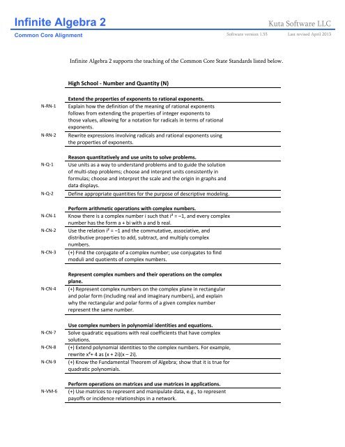
<strong>Infinite</strong> <strong>Algebra</strong> 2 supports the teaching of the <strong>Common</strong> <strong>Core</strong> State Standards listed below.<br />
High School ‐ Number and Quantity (N)<br />
N‐RN‐1<br />
N‐RN‐2<br />
N‐Q‐1<br />
N‐Q‐2<br />
N‐CN‐1<br />
N‐CN‐2<br />
N‐CN‐3<br />
N‐CN‐4<br />
N‐CN‐7<br />
N‐CN‐8<br />
N‐CN‐9<br />
N‐VM‐6<br />
Extend the properties of exponents to rational exponents.<br />
Explain how the definition of the meaning of rational exponents<br />
follows from extending the properties of integer exponents to<br />
those values, allowing for a notation for radicals in terms of rational<br />
exponents.<br />
Rewrite expressions involving radicals and rational exponents using<br />
the properties of exponents.<br />
Reason quantitatively and use units to solve problems.<br />
Use units as a way to understand problems and to guide the solution<br />
of multi‐step problems; choose and interpret units consistently in<br />
formulas; choose and interpret the scale and the origin in graphs and<br />
data displays.<br />
Define appropriate quantities for the purpose of descriptive modeling.<br />
Perform arithmetic operations with complex numbers.<br />
Know there is a complex number i such that i² = –1, and every complex<br />
number has the form a + bi with a and b real.<br />
Use the relation i² = –1 and the commutative, associative, and<br />
distributive properties to add, subtract, and multiply complex<br />
numbers.<br />
(+) Find the conjugate of a complex number; use conjugates to find<br />
moduli and quotients of complex numbers.<br />
Represent complex numbers and their operations on the complex<br />
plane.<br />
(+) Represent complex numbers on the complex plane in rectangular<br />
and polar form (including real and imaginary numbers), and explain<br />
why the rectangular and polar forms of a given complex number<br />
represent the same number.<br />
Use complex numbers in polynomial identities and equations.<br />
Solve quadratic equations with real coefficients that have complex<br />
solutions.<br />
(+) Extend polynomial identities to the complex numbers. For example,<br />
rewrite x²+ 4 as (x + 2i)(x – 2i).<br />
(+) Know the Fundamental Theorem of <strong>Algebra</strong>; show that it is true for<br />
quadratic polynomials.<br />
Perform operations on matrices and use matrices in applications.<br />
(+) Use matrices to represent and manipulate data, e.g., to represent<br />
payoffs or incidence relationships in a network.
N‐VM‐7<br />
N‐VM‐8<br />
N‐VM‐9<br />
N‐VM‐10<br />
N‐VM‐11<br />
(+) Multiply matrices by scalars to produce new matrices, e.g., as when<br />
all of the payoffs in a game are doubled.<br />
(+) Add, subtract, and multiply matrices of appropriate dimensions.<br />
(+) Understand that, unlike multiplication of numbers, matrix<br />
multiplication for square matrices is not a commutative operation, but<br />
still satisfies the associative and distributive properties.<br />
(+) Understand that the zero and identity matrices play a role in matrix<br />
addition and multiplication similar to the role of 0 and 1 in the real<br />
numbers. The determinant of a square matrix is nonzero if and only if<br />
the matrix has a multiplicative inverse.<br />
(+) Multiply a vector (regarded as a matrix with one column) by a<br />
matrix of suitable dimensions to produce another vector. Work with<br />
matrices as transformations of vectors.<br />
High School ‐ <strong>Algebra</strong> (A)<br />
A‐SSE‐1a<br />
A‐SSE‐1b<br />
A‐SSE‐2<br />
A‐SSE‐3a<br />
A‐SSE‐3b<br />
A‐SSE‐3c<br />
A‐SSE‐4<br />
A‐APR‐1<br />
Interpret the structure of expressions<br />
Interpret parts of an expression, such as terms, factors, and<br />
coefficients.<br />
Interpret complicated expressions by viewing one or more of their<br />
parts as a single entity. For example, interpret P(1+r)ⁿ as the product<br />
of P and a factor not depending on P.<br />
Use the structure of an expression to identify ways to rewrite it. For<br />
example, see x⁴ – y⁴ as (x²)²– (y²)², thus recognizing it as a difference of<br />
squares that can be factored as (x² – y²)(x² + y²).<br />
Write expressions in equivalent forms to solve problems<br />
Factor a quadratic expression to reveal the zeros of the function it<br />
defines.<br />
Complete the square in a quadratic expression to reveal the<br />
maximum or minimum value of the function it defines.<br />
Use the properties of exponents to transform expressions for<br />
exponential functions. For example the expression 1.15^t<br />
can be rewritten as (1.151/12)^(12t) ≈ 1.01212^t to reveal the<br />
approximate equivalent monthly interest rate if the annual rate is 15%.<br />
Derive the formula for the sum of a finite geometric series (when the<br />
common ratio is not 1), and use the formula to solve problems. For<br />
example, calculate mortgage payments.<br />
Perform arithmetic operations on polynomials<br />
Understand that polynomials form a system analogous to the integers,<br />
namely, they are closed under the operations of addition, subtraction,<br />
and multiplication; add, subtract, and multiply polynomials.
A‐APR‐2<br />
A‐APR‐3<br />
A‐APR‐5<br />
A‐APR‐6<br />
A‐APR‐7<br />
A‐CED‐1<br />
A‐CED‐2<br />
A‐CED‐3<br />
A‐REI‐1<br />
A‐REI‐2<br />
A‐REI‐3<br />
Understand the relationship between zeros and factors of polynomials<br />
Know and apply the Remainder Theorem: For a polynomial p(x) and a<br />
number a, the remainder on division by x – a is p(a), so p(a) = 0 if and<br />
only if (x – a) is a factor of p(x).<br />
Identify zeros of polynomials when suitable factorizations are<br />
available, and use the zeros to construct a rough graph of the function<br />
defined by the polynomial.<br />
Use polynomial identities to solve problems<br />
(+) Know and apply the Binomial Theorem for the expansion of (x + y)ⁿ<br />
in powers of x and y for a positive integer n, where x and y are<br />
any numbers, with coefficients determined for example by Pascal’s<br />
Triangle.<br />
Rewrite rational expressions<br />
Rewrite simple rational expressions in different forms; write a(x)/b(x)<br />
in the form q(x) + r(x)/b(x), where a(x), b(x), q(x), and r(x) are<br />
polynomials with the degree of r(x) less than the degree of b(x), using<br />
inspection, long division, or, for the more complicated examples, a<br />
computer algebra system.<br />
(+) Understand that rational expressions form a system analogous<br />
to the rational numbers, closed under addition, subtraction,<br />
multiplication, and division by a nonzero rational expression; add,<br />
subtract, multiply, and divide rational expressions.<br />
Create equations that describe numbers or relationships<br />
Create equations and inequalities in one variable and use them to<br />
solve problems. Include equations arising from linear and quadratic<br />
functions, and simple rational and exponential functions.<br />
Create equations in two or more variables to represent relationships<br />
between quantities; graph equations on coordinate axes with labels<br />
and scales.<br />
Represent constraints by equations or inequalities, and by systems of<br />
equations and/or inequalities, and interpret solutions as viable or nonviable<br />
options in a modeling context. For example, represent inequalities<br />
describing nutritional and cost constraints on combinations of different<br />
foods.<br />
Understand solving equations as a process of reasoning and explain<br />
the reasoning<br />
Explain each step in solving a simple equation as following from the<br />
equality of numbers asserted at the previous step, starting from the<br />
assumption that the original equation has a solution. Construct a<br />
viable argument to justify a solution method.<br />
Solve simple rational and radical equations in one variable, and give<br />
examples showing how extraneous solutions may arise.<br />
Solve equations and inequalities in one variable<br />
Solve linear equations and inequalities in one variable, including<br />
equations with coefficients represented by letters.
A‐REI‐4a<br />
A‐REI‐4b<br />
Use the method of completing the square to transform any<br />
quadratic equation in x into an equation of the form (x – p)² = q<br />
that has the same solutions. Derive the quadratic formula from<br />
this form.<br />
Solve quadratic equations by inspection (e.g., for x² = 49), taking<br />
square roots, completing the square, the quadratic formula and<br />
factoring, as appropriate to the initial form of the equation.<br />
Recognize when the quadratic formula gives complex solutions<br />
and write them as a ± bi for real numbers a and b.<br />
A‐REI‐5<br />
A‐REI‐6<br />
A‐REI‐7<br />
A‐REI‐8<br />
A‐REI‐9<br />
A‐REI‐10<br />
A‐REI‐11<br />
A‐REI‐12<br />
Solve systems of equations<br />
Prove that, given a system of two equations in two variables, replacing<br />
one equation by the sum of that equation and a multiple of the other<br />
produces a system with the same solutions.<br />
Solve systems of linear equations exactly and approximately (e.g., with<br />
graphs), focusing on pairs of linear equations in two variables.<br />
Solve a simple system consisting of a linear equation and a quadratic<br />
equation in two variables algebraically and graphically. For example,<br />
find the points of intersection between the line y = –3x and the circle x² + y² = 3.<br />
(+) Represent a system of linear equations as a single matrix equation<br />
in a vector variable.<br />
(+) Find the inverse of a matrix if it exists and use it to solve systems<br />
of linear equations (using technology for matrices of dimension 3 × 3<br />
or greater).<br />
Represent and solve equations and inequalities graphically<br />
Understand that the graph of an equation in two variables is the set of<br />
all its solutions plotted in the coordinate plane, often forming a curve<br />
(which could be a line).<br />
Explain why the x‐coordinates of the points where the graphs of<br />
the equations y = f(x) and y = g(x) intersect are the solutions of the<br />
equation f(x) = g(x); find the solutions approximately, e.g., using<br />
technology to graph the functions, make tables of values, or find<br />
successive approximations. Include cases where f(x) and/or g(x)<br />
are linear, polynomial, rational, absolute value, exponential, and<br />
logarithmic functions.<br />
Graph the solutions to a linear inequality in two variables as a halfplane<br />
(excluding the boundary in the case of a strict inequality), and<br />
graph the solution set to a system of linear inequalities in two variables<br />
as the intersection of the corresponding half‐planes.
High School ‐ Functions (F)<br />
F‐IF‐1<br />
F‐IF‐2<br />
F‐IF‐3<br />
F‐IF‐4<br />
Understand the concept of a function and use function notation<br />
Understand that a function from one set (called the domain) to<br />
another set (called the range) assigns to each element of the domain<br />
exactly one element of the range. If f is a function and x is an element<br />
of its domain, then f(x) denotes the output of f corresponding to the<br />
input x. The graph of f is the graph of the equation y = f(x).<br />
Use function notation, evaluate functions for inputs in their domains,<br />
and interpret statements that use function notation in terms of a<br />
context.<br />
Recognize that sequences are functions, sometimes defined<br />
recursively, whose domain is a subset of the integers. For example, the<br />
Fibonacci sequence is defined recursively by f(0) = f(1) = 1, f(n+1) = f(n) +<br />
f(n‐1) for n ≥ 1.<br />
Interpret functions that arise in applications in terms of the context<br />
For a function that models a relationship between two quantities,<br />
interpret key features of graphs and tables in terms of the quantities,<br />
and sketch graphs showing key features given a verbal description<br />
of the relationship. Key features include: intercepts; intervals where the<br />
function is increasing, decreasing, positive, or negative; relative maximums<br />
and minimums; symmetries; end behavior; and periodicity.<br />
F‐IF‐7a<br />
F‐IF‐7b<br />
F‐IF‐7c<br />
F‐IF‐7d<br />
F‐IF‐7e<br />
F‐IF‐8a<br />
F‐IF‐8b<br />
F‐IF‐9<br />
Analyze functions using different representations<br />
Graph linear and quadratic functions and show intercepts,<br />
maxima, and minima.<br />
Graph square root, cube root, and piecewise‐defined functions,<br />
including step functions and absolute value functions.<br />
Graph polynomial functions, identifying zeros when suitable<br />
factorizations are available, and showing end behavior.<br />
(+) Graph rational functions, identifying zeros and asymptotes<br />
when suitable factorizations are available, and showing end<br />
behavior.<br />
Graph exponential and logarithmic functions, showing intercepts<br />
and end behavior, and trigonometric functions, showing period,<br />
midline, and amplitude.<br />
Use the process of factoring and completing the square in a<br />
quadratic function to show zeros, extreme values, and symmetry<br />
of the graph, and interpret these in terms of a context.<br />
Use the properties of exponents to interpret expressions for<br />
exponential functions. For example, identify percent rate of change<br />
in functions such as y = (1.02)^t, y = (0.97)^t, y = (1.01)^(12t), y = (1.2)^(t/10), and<br />
classify them as representing exponential growth or decay<br />
Compare properties of two functions each represented in a different<br />
way (algebraically, graphically, numerically in tables, or by verbal<br />
descriptions). For example, given a graph of one quadratic function and<br />
an algebraic expression for another, say which has the larger maximum.
F‐BF‐1a<br />
F‐BF‐1c<br />
F‐BF‐2<br />
F‐BF‐3<br />
F‐BF‐4a<br />
F‐BF‐4b<br />
F‐BF‐5<br />
F‐LE‐2<br />
F‐TF‐1<br />
F‐TF‐2<br />
F‐TF‐3<br />
F‐TF‐4<br />
Build a function that models a relationship between two quantities<br />
Determine an explicit expression, a recursive process, or steps for<br />
calculation from a context.<br />
(+) Compose functions. For example, if T(y) is the temperature in<br />
the atmosphere as a function of height, and h(t) is the height of a<br />
weather balloon as a function of time, then T(h(t)) is the temperature<br />
at the location of the weather balloon as a function of time.<br />
Write arithmetic and geometric sequences both recursively and<br />
with an explicit formula, use them to model situations, and translate<br />
between the two forms.<br />
Build new functions from existing functions<br />
Identify the effect on the graph of replacing f(x) by f(x) + k, k f(x),<br />
f(kx), and f(x + k) for specific values of k (both positive and negative);<br />
find the value of k given the graphs. Experiment with cases and<br />
illustrate an explanation of the effects on the graph using technology.<br />
Include recognizing even and odd functions from their graphs and<br />
algebraic expressions for them.<br />
Solve an equation of the form f(x) = c for a simple function f<br />
that has an inverse and write an expression for the inverse. For<br />
example, f(x) =2x³ or f(x) = (x+1)/(x–1) for x ≠ 1.<br />
(+) Verify by composition that one function is the inverse of<br />
another.<br />
(+) Understand the inverse relationship between exponents and<br />
logarithms and use this relationship to solve problems involving<br />
logarithms and exponents.<br />
Construct and compare linear, quadratic, and exponential models<br />
and solve problems<br />
Construct linear and exponential functions, including arithmetic and<br />
geometric sequences, given a graph, a description of a relationship, or<br />
two input‐output pairs (include reading these from a table).<br />
Extend the domain of trigonometric functions using the unit circle<br />
Understand radian measure of an angle as the length of the arc on the<br />
unit circle subtended by the angle.<br />
Explain how the unit circle in the coordinate plane enables the<br />
extension of trigonometric functions to all real numbers, interpreted as<br />
radian measures of angles traversed counterclockwise around the unit<br />
circle.<br />
(+) Use special triangles to determine geometrically the values of sine,<br />
cosine, tangent for π/3, π/4 and π/6, and use the unit circle to express<br />
the values of sine, cosine, and tangent for π–x, π+x, and 2π–x in terms<br />
of their values for x, where x is any real number.<br />
(+) Use the unit circle to explain symmetry (odd and even) and<br />
periodicity of trigonometric functions.
F‐TF‐6<br />
F‐TF‐9<br />
Model periodic phenomena with trigonometric functions<br />
(+) Understand that restricting a trigonometric function to a domain<br />
on which it is always increasing or always decreasing allows its inverse<br />
to be constructed.<br />
Prove and apply trigonometric identities<br />
(+) Prove the addition and subtraction formulas for sine, cosine, and<br />
tangent and use them to solve problems.<br />
High School ‐ Geometry (G)<br />
G‐CO‐2<br />
G‐CO‐3<br />
G‐CO‐5<br />
G‐CO‐6<br />
G‐SRT‐6<br />
G‐SRT‐7<br />
G‐SRT‐8<br />
G‐SRT‐10<br />
G‐SRT‐11<br />
Experiment with transformations in the plane<br />
Represent transformations in the plane using, e.g., transparencies<br />
and geometry software; describe transformations as functions that<br />
take points in the plane as inputs and give other points as outputs.<br />
Compare transformations that preserve distance and angle to those<br />
that do not (e.g., translation versus horizontal stretch).<br />
Given a rectangle, parallelogram, trapezoid, or regular polygon,<br />
describe the rotations and reflections that carry it onto itself.<br />
Given a geometric figure and a rotation, reflection, or translation,<br />
draw the transformed figure using, e.g., graph paper, tracing paper, or<br />
geometry software. Specify a sequence of transformations that will<br />
carry a given figure onto another.<br />
Understand congruence in terms of rigid motions<br />
Use geometric descriptions of rigid motions to transform figures and<br />
to predict the effect of a given rigid motion on a given figure; given<br />
two figures, use the definition of congruence in terms of rigid motions<br />
to decide if they are congruent.<br />
Define trigonometric ratios and solve problems involving right triangles<br />
Understand that by similarity, side ratios in right triangles are<br />
properties of the angles in the triangle, leading to definitions of<br />
trigonometric ratios for acute angles.<br />
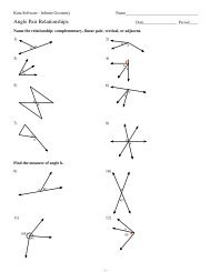
Explain and use the relationship between the sine and cosine of<br />
complementary angles.<br />
Use trigonometric ratios and the Pythagorean Theorem to solve right<br />
triangles in applied problems.<br />
Apply trigonometry to general triangles<br />
(+) Prove the Laws of Sines and Cosines and use them to solve<br />
problems.<br />
(+) Understand and apply the Law of Sines and the Law of Cosines<br />
to find unknown measurements in right and non‐right triangles (e.g.,<br />
surveying problems, resultant forces).
G‐C‐5<br />
G‐GPE‐1<br />
G‐GPE‐2<br />
G‐GPE‐3<br />
G‐GPE‐5<br />
Find arc lengths and areas of sectors of circles<br />
Derive using similarity the fact that the length of the arc intercepted<br />
by an angle is proportional to the radius, and define the radian<br />
measure of the angle as the constant of proportionality; derive the<br />
formula for the area of a sector.<br />
Translate between the geometric description and the equation for a<br />
conic section<br />
Derive the equation of a circle of given center and radius using the<br />
Pythagorean Theorem; complete the square to find the center and<br />
radius of a circle given by an equation.<br />
Derive the equation of a parabola given a focus and directrix.<br />
(+) Derive the equations of ellipses and hyperbolas given the foci,<br />
using the fact that the sum or difference of distances from the foci is<br />
constant.<br />
Use coordinates to prove simple geometric theorems algebraically<br />
Prove the slope criteria for parallel and perpendicular lines and use<br />
them to solve geometric problems (e.g., find the equation of a line<br />
parallel or perpendicular to a given line that passes through a given<br />
point).<br />
Standards from www.corestandards.org/assets/CCSSI_Math%20Standards.pdf<br />
Standards are © Copyright 2010. National Governors Association Center for Best Practices and<br />
Council of Chief State School Officers. All rights reserved.