The Xmath Partial Differentiation Algorithm

REPLACE THIS LINE WITH YOUR PAPER IDENTIFICATION NUMBER (DOUBLE-CLICK HERE TO 

EDIT) < 

1 

The Xmath Partial Differentiation Algorithm 

Odd Bringslid 

Abstract—The Xmath eBook is being 

developed and algorithms into a wide range 

of undergraduate mathematical issues 

embeded in Mathematica packages are 

available on the web using the system 

webMathematica. The main purpose is to 

visualize mathematics in the same way as 

would a professor do it on the blackboard 

stating all intermediate steps for user defined 

input and then presenting solutions being 

easily recognized by the undegraduate 

student which may not always be the case 

using the Mathematica system directly. In this 

way the student may work more on a personal 

basis, viewing one step at a time in the 

solving process and then being less 

dependent of the professors. In this paper 

The Xmath Algorithm for Partial 

Differentiation step-by-step are presented (PD 

Steplet) 

Index Terms— Partial Differentiation (PD), 

Steplet, Mathematica packages, Online 

calculations, Pedagogical value 

T 

1. INTRODUCTION 

he use of Mathematica [1] in education is one 

of the most important areas of application. 

The problem however is that in education we are 

focusing on how problems are solved perhaps 

more than on the final result. Since Mathematica 

only gives the final result it will be necessary to 

build an application on top of Mathematica giving 

intermediate results using the methods of solving 

given by mathematical textbooks. It is necessary 

to analyze the equations in depth, Xmath then 

using the Mathematica object TreeForm to be 

able to extract the information needed at each 

level of the solution process. The algorithm is 

different from the algorithm used by the 

developers of the Mathematica System (D). 

The Xmath algorithm will solve problems typical 

in mathematical teaching. General partial 

differentiation is implemented using standard 

methods, tracking the solving process in detail to 

be easily recognized by the students. 

 

Manuscript received 2010. Author, assoc. prof. Odd Bringslid 

is with the Institute of technology, Buskerud University College, 

Norway (odd.bringslid@hibu.no) 

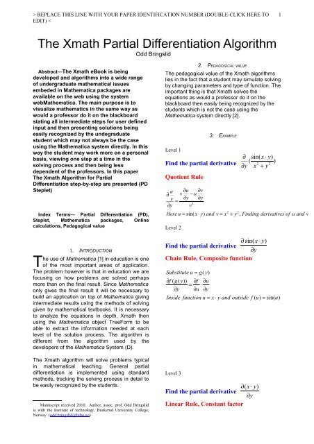
2. PEDAGOGICAL VALUE 

The pedagogical value of the Xmath algorithms 

lies in the fact that a student may simulate solving 

by changing parameters and type of function. The 

important thing is that Xmath solves the 

equations as would a professor do it on the 

blackboard then easily being recognized by the 

students which is not the case using the 

Mathematica system directly [2]. 

Level 1 

3. EXAMPLE 

Find the partial derivative 

Quotient Rule 

u ∂u 

∂v 

∂ v − u 

v ∂y 

∂y 

= 

2 

∂y 

v 

2 2 

Here u sin( x y) and v x y , Finding derivatives of u and v 

Level 2 

= ⋅ = + 

∂ sin( x ⋅ y) 


∂y 

Chain Rule, Composite function 

Substitute u = g( y) 

∂f ( g( y)) 

∂f ∂u 

= ⋅ 

∂y ∂u ∂y 

Inside function u = x ⋅ y and outside f ( u) = sin( u) 

Level 3 

∂ sin( x ⋅ y) 

( ) 

2 2 

∂ y x + y 

∂( x ⋅ y) 


∂y 

Linear Rule, Constant factor


EDIT) < 

2 

∂( c ⋅ f ) ∂f 

= c ⋅ , Here c = x and f ( y) 

= y 

∂y 

∂y 

Finding the derivative of the non − constant factor f ( y) 

= 

Level 4 

2 2 2 2 

∂ ( x + y ) ∂x ∂y 

= + 

∂y ∂y ∂y 

Level 3 


Power Rule 

n 

∂y 

∂y 

∂ y = 1 

∂y 

n− 

= n ⋅ y 

1 , Here n = 1 

∂y 

∂y 

2 

∂x 


∂y 

Constant Rule 

Derivative of a constant is 0 (independent of y) 

2 

∂x 

∂y 

= 0 

Result, Linear Rule Constant factor 

∂( x ⋅ y) 

∂y 

= x = x 

∂y 

∂y 

∂ u = x 

∂y 

Finding the dervative of the outside function 

Level 3 


Sin Rule 

∂ sin( u) 

= cos( u) 

∂u 

∂ f = cos( u) 

∂u 

∂ sin( u) 

∂u 

Result, Linear Rule Sum 

2 2 2 2 

∂ ( x + y ) ∂y ∂x 

= + = 2y 

∂y ∂y ∂y 

∂v 

∂v 

This gives = 2y and u = 2y sin( x ⋅ y) 

∂y 

∂y 

in the second part of numerator of the rule. 

We then find the numerator : 

∂u 

∂v 

v − u = x x + y x ⋅ y − y ⋅ sin x ⋅ y 

∂y 

∂y 

Result, Quotient Rule (Answer) 

sin( x ⋅ y) 

∂u ∂v 

∂ v − u 

2 2 

x + y ∂y ∂y 

= = 

2 

∂y 

v 

2 2 

( )cos( ) 2 ( ) 

x x y x y y x y 

2 2 2 

( x + y ) 

2 2 

( + )cos( ⋅ ) − 2 sin( ⋅ ) 

Result, Chain Rule 

Substitute u = g( y) 

= x ⋅ y 

∂ sin( x ⋅ y) ∂( g( y)) 

∂f ∂u 

= = = x ⋅cos( x ⋅ y) 

∂y ∂y ∂u ∂y 

∂u 

∂u 

This gives = x ⋅ x ⋅ y and v = x x + y x ⋅ y 

∂y 

∂y 

Level 2 


Linear Rule, Sum 

2 2 

cos( ) ( )cos( ) 

∂ + 

∂y 

2 2 

( x y ) 

4. THE LINEAR RULE 

The linear rule will differentiate a function like 

(1) f ( x , x ,..) = a f ( x , x ,..) + a f ( x , x ,..) + ... 

1 2 1 1 1 2 2 2 1 2 

Here a 

i is independent of x. The rule is divided 

into the linear rule sum and the linear rule 

consant factor.


EDIT) < 

3 

The function is broken down for analyzing by 

using the Mathematica object TreeForm [3] with 2 

levels. The Mathematica object D [4] gives the 

derivative. Linear rule sum: 

LinearList=Reverse[Level[TreeForm[f],2]]; 

LinearList=Delete[LinearList,1]; 

Do[Main[ak*yk,level],{j,1,Length[LinearList]}] 

] (*end Do*)); 

Result=Sum[Main[ak*yk]] 

Figure 1 PseudoCode Linear Rule Sum 

FactList=Reverse[ 

Level[TreeForm[a*y[x]],2]]; 

If [ FreeQ[FactList[[3]],x], 

Result=FactList[[3]] * Main[FactList[[2]],x,level]] 

Figure 2 PseudoCode Linear Rule Constant Factor 

Head[expr]===Plus,DPlusRule[expr,x,level] 

Head[expr]===Times&&(Not[FreeQ[Denominator[ 

k[[2]]],x]] 

ν Not[FreeQ[Denominator[k[[3]]],x]]), 

DQuotRule[expr,x,level], 

Head[expr]===Times&&FreeQ[Last[k],x] ν 

FreeQ[k[[2]],x],DProdCoRule[expr,x,level], 

Head[expr[===Times, DProductRule[expr,x,level], 

Head[expr]===Power&&k[[3]]===x&&FreeQ[k[[2]],x],DPower 

Rule[expr,x,level], 

Head[expr]===Power&&FreeQ[k[[2]],x],DChainRule[expr,x,lev 

el], 

Head[expr]===Power&&Head[k[[2]]]===Symbol&&FreeQ[k[[3] 

],x], 

DDPowerRuleExp[expr,x,level], 

5. THE QUOTIENT RULE 

The quotient rule will differentiate a function like 

u( x , x ,...) 

(2) f ( x , x ,...) = 

1 2 

1 2 

v( x1, x2,...) 

expr=u/v; 

u=Numerator[expr]; 

v=Denominator[expr]; 

Result=Main[D[u,x]*v-D[v.x]*u)/v^2,level]; 

Figure 3 PseudoCode QutientRule 

6. CHAIN RULE 

This rule is used for a function being a composite 

function of the form y=f (g(x)). The derivative is 

given by the chain rule 

u = g( x) 

∂f ( g( x)) ∂f ( u) 

∂u 

= ⋅ 

∂x ∂u ∂x 

expr=g[u[x]]; 

u=Reverse[Level[TreeForm[g[u[x]], 2]]; 

Result=Main[D[expD[g[u],u]*D[u[x]]; 

Figure 4 PseudoCode ChainRule 

MAIN PROGRAM 

PseudoCode given for rules used in the eaxmple. 

Main[expr,x,level]:=Module[{}, 

k=Reverse[Level[TreeForm[e …)xpr,2]; 

Which[ 

FreeQ[expr,x],DConstantRule[expr,x,level], 

expr===x,DxRule[expr,x,level], 

Head[expr]===Tan, 

If[Last[k]===x,DTanRule[expr,x,level],DChainRule[expr,x,level 

]], 

(* Same system for 

Cos,Sin,Log,Arctan,ArcSin,ArcCos*) 

FreeQ[k[[3]],x]&&Head[expr]=Power,DChainRuleExp[expr,x,le 

vel], 

Head[expr]==Power&&Not[FreeQ[k[[2]],x]], 

LogarithmicRule[expr,x,level] 

] 

Figure 5 PseudoCode Main Program 

The Main Program invokes the Mathemaica objects 

FreeQ [5], Head[6], Which[7] and Reverse [8] 

ACKNOWLEDGMENT 

Acknowledgements are expressed to the 

partners of the EU projects Xmath [9] and dMath 

[10]. 

REFERENCES 

[1] Wolfram Research, http://www.wolfram.com/ 

[2] Bringslid, Odd, Norstein, Anne (2008), Teaching 

Mathematics using Steplets. International Journal of 

Mathematical Education in Science and Technology 

39:7 pp 925-936 

[3] Wolfram Research, The Mathematica Book (2003) pp 

236-237 


80 


124 


231 


345 


127 

[9] Xmath project (http://dmath.hibu.no/xmath/) 

[10] dMath project (http://dmath.hibu.no) 

Odd Bringslid 

Assoc. Professor at The Institute of Technology, Buskerud 

University College, Norway. Project coordinator of EU 

Leonardo project dMath [1], EU Minerva project Xmath [4] 

and a former third party program designer for HP calculators.


EDIT) < 

4 

Officially appointed as Project leader of Educational 

Government Projects. Partner in the JEM project. Conference 

leader of several European Conferences into eLearning. 

Guest Editor of the Journal of Computers in Mathematics and 

Science Teaching. Research into mathematical eLearning 

and Computer Algebra and proposed Member of the 

OpenMath Society.

The Xmath Partial Differentiation Algorithm

Create successful ePaper yourself

Delete template?

Save as template?