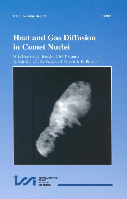
Heat and Gas Diffusion in Comet Nuclei (pdf file 5.5 MB) - ISSI

HEAT AND GAS DIFFUSION IN
COMET NUCLEI
Walter F. Huebner
Southwest Research Institute, USA
Johannes Benkhoff 1
Institute for Planetary Research, DLR-Berlin, Germany
Maria-Teresa Capria, Angioletta Coradini,
Christina De Sanctis, Roberto Orosei
Istituto di Astrofisica Spaziale, Italy
Dina Prialnik
Tel Aviv University, Israel
August 8, 2006
1 Presently with Research and Scientific Support Department, ESA-ESTEC, The
Netherlands

Contents
Foreword
Preface
xv
xvii
1 Introduction – Observational Overview 1
2 The Structure of Comet Nuclei 9
2.1 Size and Composition . . . . . . . . . . . . . . . . . . . . . . 9
2.2 Some Physical Properties . . . . . . . . . . . . . . . . . . . . 15
2.3 Comet – Asteroid Transitions . . . . . . . . . . . . . . . . . . 19
2.4 Laboratory Simulations . . . . . . . . . . . . . . . . . . . . . 21
2.4.1 KOSI Experiments . . . . . . . . . . . . . . . . . . . . 21
2.4.2 Cometary Materials: the Effects of Bombardment with
Energetic Charged Particles . . . . . . . . . . . . . . . 23
2.4.3 Experiments on Gas Trapping . . . . . . . . . . . . . . 24
2.4.4 Measurements of Thermal Conductivity . . . . . . . . 25
2.4.5 Other Laboratory Measurements . . . . . . . . . . . . 28
3 Physical Processes in Comet Nuclei 31
3.1 Sublimation of Ices . . . . . . . . . . . . . . . . . . . . . . . 32
3.2 The Phase Transition of Amorphous Ice . . . . . . . . . . . . 33
3.3 Gas Diffusion in Pores . . . . . . . . . . . . . . . . . . . . . . 35
3.3.1 Comments on Porosity . . . . . . . . . . . . . . . . . 35
3.3.2 The Surface-to-Volume Ratio . . . . . . . . . . . . . . 37
3.3.3 Gas Flow . . . . . . . . . . . . . . . . . . . . . . . . . 39
3.4 The Coma/Nucleus Boundary Layer . . . . . . . . . . . . . . 41
3.4.1 The Knudsen Layer in the Coma . . . . . . . . . . . . 41
3.4.2 Effects of Nucleus Surface Topography . . . . . . . . . 46
3.5 Dust Entrainment and Dust Mantling . . . . . . . . . . . . . 48
3.5.1 The Critical Dust Particle Size . . . . . . . . . . . . . 49
3.5.2 Models of Dust Mantle Formation . . . . . . . . . . . 50
3.5.3 Porosity of the Dust Mantle . . . . . . . . . . . . . . 51
3.6 Fracturing, Splitting, and Outbursts . . . . . . . . . . . . . . 53
4 Basic Equations 57
4.1 Mass Balance . . . . . . . . . . . . . . . . . . . . . . . . . . . 57
4.2 Energy Balance . . . . . . . . . . . . . . . . . . . . . . . . . . 59
4.3 Momentum Balance . . . . . . . . . . . . . . . . . . . . . . . 61
iii

iv
Contents
4.4 Boundary Conditions . . . . . . . . . . . . . . . . . . . . . . . 61
4.5 Initial Structure and Parameters . . . . . . . . . . . . . . . . 63
4.6 Flow Regimes and their Transitions . . . . . . . . . . . . . . . 66
4.7 Dust Flow and Mantling . . . . . . . . . . . . . . . . . . . . . 68
4.8 Sublimation and Condensation in Pores . . . . . . . . . . . . 72
4.9 Effective Thermal Conductivity . . . . . . . . . . . . . . . . 73
5 Analytical Considerations 79
5.1 Early Models . . . . . . . . . . . . . . . . . . . . . . . . . . . 79
5.2 Characteristic Properties of the Nucleus . . . . . . . . . . . . 84
5.3 Characteristic Timescales . . . . . . . . . . . . . . . . . . . . 86
5.3.1 The Surface Temperature . . . . . . . . . . . . . . . . 87
5.3.2 The Onset of Crystallization . . . . . . . . . . . . . . 89
5.3.3 Fracture Instability . . . . . . . . . . . . . . . . . . . . 90
5.3.4 The Effect of Radioactivity . . . . . . . . . . . . . . . 90
5.4 An Analytical Model for Crystallization and its Implications . 91
5.4.1 A Two-Zone Model . . . . . . . . . . . . . . . . . . . . 92
5.4.2 Implications for the Onset of Cometary Activity . . . 95
5.4.3 The Intermittent Progress of Crystallization . . . . . . 97
6 Numerical Methods 99
6.1 1-D Difference Schemes . . . . . . . . . . . . . . . . . . . . . 99
6.2 Treatment of Boundary Conditions . . . . . . . . . . . . . . . 103
6.3 From 1-D to Multi-Dimensions . . . . . . . . . . . . . . . . . 107
6.4 Simultaneous Solution for Transfer of Heat and Mass . . . . . 109
6.5 Stability Problems . . . . . . . . . . . . . . . . . . . . . . . . 111
7 Comparison of Algorithms 115
7.1 Rationale . . . . . . . . . . . . . . . . . . . . . . . . . . . . . 115
7.2 Thermal Algorithm: Different Formulations . . . . . . . . . . 118
7.3 The Models . . . . . . . . . . . . . . . . . . . . . . . . . . . . 120
7.4 Results of Different Algorithms for Various Models . . . . . . 121
7.5 Conclusions . . . . . . . . . . . . . . . . . . . . . . . . . . . . 131
8 Orbital Effects 135
8.1 Inward Heat Flux . . . . . . . . . . . . . . . . . . . . . . . . 135
8.2 Short-Period vs. Long-Period Comets . . . . . . . . . . . . . 137
8.2.1 Dynamical Evolution . . . . . . . . . . . . . . . . . . . 137
8.2.2 Differences between Long- and Short-Period Comets . 140
8.3 Changing Orbits . . . . . . . . . . . . . . . . . . . . . . . . . 144
8.4 Multistage or Direct Injection . . . . . . . . . . . . . . . . . . 146
8.5 Sungrazing Comets . . . . . . . . . . . . . . . . . . . . . . . . 147

v
9 Spin Effects 151
9.1 Diurnal Evolution . . . . . . . . . . . . . . . . . . . . . . . . 151
9.2 Gas Emission . . . . . . . . . . . . . . . . . . . . . . . . . . . 151
9.3 Day – Night Temperature Difference . . . . . . . . . . . . . . 153
9.4 Effect of Spin Axis Inclination . . . . . . . . . . . . . . . . . 155
9.4.1 Uneven Distribution of Dust Mantles . . . . . . . . . . 155
9.4.2 Uneven Erosion . . . . . . . . . . . . . . . . . . . . . . 158
9.5 Effect of Spin Rate . . . . . . . . . . . . . . . . . . . . . . . . 160
10 Comparison of Models with Observations 165
10.1 Modeling Guided by Observations . . . . . . . . . . . . . . . 165
10.1.1 Example 1: Comet Hale-Bopp (C/1995 O1) . . . . . . 165
10.1.2 Example 2: Comet 46P/Wirtanen . . . . . . . . . . . 174
10.2 Conclusions Based on Multiple Simulations . . . . . . . . . . 181
10.3 Comet Outbursts . . . . . . . . . . . . . . . . . . . . . . . . . 184
10.3.1 Distant Outbursts of Comet 1P/Halley . . . . . . . . 186
10.3.2 Pre-Perihelion Activity of 2060 Chiron . . . . . . . . . 186
10.3.3 Erratic Activity of 29P/Schwassmann-Wachmann 1 . 187
10.3.4 Distant Activity of Comet Hale-Bopp (C/1995 O1) . . 188
10.4 Coma Versus Nucleus Abundances . . . . . . . . . . . . . . . 188
10.4.1 Multi-Volatile Model of Comet
67P/Churyumov-Gerasimenko . . . . . . . . . . . . . 188
10.4.2 Volatile Production Rates Compared with Nucleus
Composition . . . . . . . . . . . . . . . . . . . . . . . 192
11 Internal Properties of Comet Nuclei 197
11.1 Temperature Profiles . . . . . . . . . . . . . . . . . . . . . . . 197
11.2 Stratification of Composition . . . . . . . . . . . . . . . . . . 198
11.3 Dust Mantle Thickness . . . . . . . . . . . . . . . . . . . . . . 201
12 Conclusions 205
12.1 Numerical Algorithms . . . . . . . . . . . . . . . . . . . . . . 206
12.2 Goals of Comet Nucleus Modeling . . . . . . . . . . . . . . . 206
12.2.1 Derivation of Internal Properties . . . . . . . . . . . . 207
12.2.2 Identification of Internal Processes . . . . . . . . . . . 208
12.3 General Characteristics of Comet Nuclei . . . . . . . . . . . . 208
12.4 General Behaviour Patterns . . . . . . . . . . . . . . . . . . . 209
12.5 Input Data Required from Observations and Experiments . . 210
12.5.1 Recommended Advances for Numerical Modeling . . . 213
12.5.2 Physical Processes . . . . . . . . . . . . . . . . . . . . 213
12.5.3 Modeling the Evolution of Comet Nuclei . . . . . . . . 213

vi
Contents
Appendix A: Orbital Parameters and Sizes of Comet Nuclei 215
Appendix B: Thermodynamic Properties 221
B.1 Vapour Pressures and Changes in Enthalpy of Sublimation . 221
B.2 Specific Heat . . . . . . . . . . . . . . . . . . . . . . . . . . . 223
B.3 Thermal conductivity . . . . . . . . . . . . . . . . . . . . . . 223
B.4 Phase Transitions . . . . . . . . . . . . . . . . . . . . . . . . . 224
Glossary 225
Bibliography 227
Index 253

List of Figures
1.1 Four comet nuclei visited by spacecraft. Top left: The nucleus
of Comet 1P/Halley is about 15.5 × 8.5 × 8 km in size. The
best spatial resolution (2 pixels) is about 100 m at the top
part of the image as obtained by the Halley Multicolour Camera
on the Giotto spacecraft (Courtesy H.U. Keller; copyright
1986 MPAE). Top right: The nucleus of Comet 19P/Borrelly
is about 16 × 8 × 8 km in size. Spatial resolution (2 pixels)
over most of the image is about 90 m. The image was
obtained with the Miniature Imaging Camera and Spectrometer
(Courtesy L. Soderblom). Bottom left: The nucleus of
Comet 81P/Wild is about 5.5 × 4.0 × 3.3 km in size. The
spatial resolution (2 pixels) is about 20 m as obtained by
the Stardust mission (Courtesy R. Newburn). Bottom right:
A composite of many images from the Impactor Targeting
Sensor of the Deep Impact mission on approach to the nucleus
of 9P/Tempel 1. The nucleus is about 6.2 × 4.6 km in
size. Highest resolution, approximately 2-3 metres, is in the
area near the impact site, where small, sub-frame, close-up
images were obtained. The resolution gradually degrades toward
the edges of the frame (Courtesy Deep Impact Project.
Image processing by A. Delamere and D. Stern). . . . . . . . 3
3.1 Hexagonal packing of spheres . . . . . . . . . . . . . . . . . . 37
4.1 Thermal conductivity correction formulae: parallel combination
(par), series combination (ser), geometrical mean (geo),
Maxwell upper limit (Max U ) and lower limit (Max L ). Results
are given for two ice to pore ratios: solid lines for the
higher ratio(s), and dotted lines for the lower one (d). The
green line represents the Monte Carlo fractal model. . . . . . 78
vii

viii
List of Figures
5.1 Change in enthalpy of sublimation of water ice. The black
dashed curve is the change in enthalpy of sublimation of water
ice under equilibrium conditions (Gibbins, 1990). The
solid red curve presents this correct change in enthalpy of
sublimation into vacuum. The green squares represent the
change in enthalpy for sublimation into vacuum as obtained
by Delsemme and Miller (1971) based on data from Washburn
(1928). Note that two points are outside the limits of validity
of the Washburn data, indicated by blue triangles. The blue
dashed curve is the fit by Cowan and A’Hearn (1979) to the
data of Delsemme and Miller. The black dotted curve has
been corrected twice for sublimation into vacuum using the
data of Gibbins. The similarity between the blue and black
dotted curves leads us to believe that Delsemme and Miller
made the correction twice. . . . . . . . . . . . . . . . . . . . . 81
5.2 Net flux and surface temperature for sublimation of H 2 O ice,
in terms of the molecular flux, Z H2 O = Q H2 O/m H2 O, where
m H2 O is the mass of a water molecule. . . . . . . . . . . . . . 83
5.3 Timescales of different evolutionary processes (see text) as
a function of temperature for different cases: (top) 1 m at
1 AU; (middle) 10 m at 10 AU; (bottom) 1000 m at 1000 AU. 88
5.4 Schematic representation of the two-zone model . . . . . . . . 93
5.5 Regions of dominance of the two energy sources: insolation
and crystallization of amorphous ice, as a function of initial
comet temperature T 0 and heliocentric distance, r H ; ɛ is the
emissivity. . . . . . . . . . . . . . . . . . . . . . . . . . . . . 96
6.1 Numerical grid. T c is the central temperature, which corresponds
to T 0 in the text. The F i are the fluxes crossing
boundaries. . . . . . . . . . . . . . . . . . . . . . . . . . . . . 100
6.2 Daily variation of surface temperature at aphelion as a function
of the phase angle from the local meridian, for the temperature
surface boundary conditions Eq. (4.25) (solid line)
and Eq. (6.20) (dashed line). . . . . . . . . . . . . . . . . . . 105
6.3 Daily variation of surface temperature at aphelion as a function
of the phase angle from the local meridian, for the temperature
surface boundary conditions Eq. (4.25) (solid line)
and Eq. (6.20) (dashed line) and for a surface layer thickness
of 5 mm. The curves of Fig. 6.2 are shown as dotted lines for
reference. . . . . . . . . . . . . . . . . . . . . . . . . . . . . . 107

ix
6.4 Schematic representation of numerical grids for a spinning
nucleus, commonly used in model calculations. Dots indicate
radial directions along which heat conduction is computed;
only in the 2.5-D model is lateral conduction included, and
only along the meridian, as shown. . . . . . . . . . . . . . . . 108
6.5 Flowchart for an implicit comet nucleus evolution code. . . . 110
7.1 Temperature as a function of time. Results obtained from
five different algorithms of Model 1: Algorithm A (solid line),
algorithm B (short broken line), algorithm C1 (long broken
line), algorithm C2 (dash-dot line), and algorithm D (dotted
line). . . . . . . . . . . . . . . . . . . . . . . . . . . . . . . . . 122
7.2 Water flux as a function of time. Results from five different
algorithms of Model 1 (see Fig. 7.1). . . . . . . . . . . . . . . 124
7.3 Decay of the water ice surface and the location of CO sublimation
front as a function of time for Model 3a. . . . . . . . 125
7.4 CO flux as a function of time. Results from different algorithms
of Model 3a (see Fig. 7.1). . . . . . . . . . . . . . . . . 125
7.5 Temperature as a function of time. Results from five different
algorithms of Model 4a (see Fig. 7.1). . . . . . . . . . . . . . 127
7.6 Water flux as a function of time. Results from four different
algorithms for Model 4a (see Fig. 7.1). . . . . . . . . . . . . . 127
7.7 CO flux as a function of time. Results of two different algorithms
(B and C2) of Model 4a (see Fig. 7.1). . . . . . . . . . 129
8.1 Comparison of heat flux for a fast spinning and a slowly spinning
comet nucleus in the orbit of 46P/Wirtanen. Negative
flux values indicate that the flux is outflowing. (From Cohen
et al., 2003.) . . . . . . . . . . . . . . . . . . . . . . . . . . . . 136
8.2 Difference between surface temperature of a fast spinning nucleus
and daily average of a slowly spinning nucleus versus heliocentric
distance, with the Hertz factor as parameter (from
Cohen et al., 2003). . . . . . . . . . . . . . . . . . . . . . . . . 137
9.1 Energy flux at the nucleus surface for insolation, reradiation
in the infrared, water ice sublimation, and conduction into
the interior as a function of subsolar angle ζ, at heliocentric
distance r H = 1.1 AU. . . . . . . . . . . . . . . . . . . . . . . 152
9.2 Diurnal evolution of gas emissions over a spin period of 3
hours. Water (solid line) and CO (dashed line) fluxes computed
from algorithm C1 with parameters given in Table 7.4. 153

x
List of Figures
9.3 Model of 46P/Wirtanen: temperature distribution throughout
an outer layer in the equatorial plane of the spinning
nucleus (P spin = 24 h). The geometry is distorted, as the nucleus
bulk is represented by a central, isothermal point mass
and only the outermost 2 m around the equator are shown.
(Adapted from Cohen et al., 2003.) . . . . . . . . . . . . . . . 154
9.4 Same as Fig. 9.3, for a comet in the orbit of 1P/Halley, with
P spin = 72 h, with the bulk of the nucleus represented again
by a central point mass. Note that the temperature distribution
is shown down to a depth of 3 m at perihelion, and 80 m
at aphelion. . . . . . . . . . . . . . . . . . . . . . . . . . . . . 156
9.5 Day to night temperature differences vs. subsolar temperature
for three different Hertz factors (from Cohen et al., 2003).157
9.6 Model for the shape evolution of an initially spherical nucleus
in the orbit of Comet 46P/Wirtanen (Cohen et al., 2003),
assuming uniform erosion, i.e. no inactive areas. The inclination
of the spin axis to the orbital plane is: 90 ◦ (left)
and 45 ◦ (right). In the latter case, the spin axis is in the
plane perpendicular to the orbital plane and contains the apsidal
direction. The shape of the comet is projected on a
2-dimensional plane. Axis labels are given in metres . . . . . 160
9.7 Diurnal temperatures for a model with a spin period of 3
hours. Solid line: surface temperature, dotted line: CO 2 ice
sublimation front; dash-dotted line: amorphous - crystalline
ice interface; dashed line: CO ice sublimation front. . . . . . . 163
9.8 Same as Fig. 9.7, except the spin period is 3 days. . . . . . . 163
10.1 Models for the production rates of Comet Hale-Bopp (C/1995
O1) based on different assumptions: Model 1 from Table 10.1.
Upper panel: slow release of CO gas from amorphous water
ice. Lower panel: instantaneous release of CO gas. . . . . . . 168
10.2 Models for gas and dust release rates of Comet Hale-Bopp
(C/1995 O1) based on different assumptions. Model 2 from
Table 10.1. Upper panel: slow release of CO gas from amorphous
water ice. Lower panel: instantaneous release of CO
gas. . . . . . . . . . . . . . . . . . . . . . . . . . . . . . . . . 169
10.3 Gas production rates along one orbit of Comet Hale-Bopp
(C/1995 O1): continuous and dashed-dotted lines represent,
respectively, CO and water production rates obtained from
the model, while triangles represent CO production from observation.
The vertical line marks the perihelion. . . . . . . . 174

xi
10.4 Flux rates of H 2 O, CO 2 , and CO along an orbit of Comet
P/Wirtanen. . . . . . . . . . . . . . . . . . . . . . . . . . . . 175
10.5 Maximum (solid line) and minimum (dashed-dotted line) daily
temperatures from aphelion to perihelion at the surface of a
bare (no dust mantle ) comet nucleus in the orbit of Comet
46P/Wirtanen. . . . . . . . . . . . . . . . . . . . . . . . . . . 177
10.6 Model of comet 46P/Wirtanen: Maximum and minimum
daily temperatures (solid lines) from aphelion to perihelion
for a surface covered by a dust mantle (model A in text). The
dashed-dotted line represents the temperature of the water
sublimation front below the dust mantle. . . . . . . . . . . . 179
10.7 Maximum and minimum daily temperatures (solid lines) from
aphelion to perihelion for a surface covered by a dust mantle
(model B). The dashed-dotted line represents the temperature
of the water sublimation front. . . . . . . . . . . . . . . . 180
10.8 Map of the surface temperature of Comet 9P/Tempel 1 prior
to impact. The scale is 160 m/pixel. Temperatures range
from about 260 K to about 330 K on the sunlit portion of
the nucleus. The temperature closely follows the topography,
demonstrating the low thermal inertia of the body. (Courtesy
Deep Impact Project. Analysis and map by O. Groussin). . . 182
10.9 Mass fluxes of H 2 O, CO, CO 2 , CH 3 OH, HCN, H 2 S, C 2 H 2 ,
C 2 H 6 and CH 4 from the surface as a function of heliocentric
distance for models assuming a heat conductivity of 0.01
times the conductivity of pure water ice. . . . . . . . . . . . . 189
10.10Mass fluxes of H 2 O, CO, CO 2 , CH 3 OH, HCN, H 2 S, C 2 H 2 ,
C 2 H 6 and CH 4 from the surface as a function of heliocentric
distance for models assuming a heat conductivity of 0.01
times the conductivity of pure water. Fluxes originate from
a belt of ±10 ◦ around latitude 60 ◦ . . . . . . . . . . . . . . . . 190
10.11Production rates for one orbital revolution: red – CO; magenta
– CO 2 ; green – CH 4 ; cyan – HCN; black – NH 3 . Models,
as listed in Table 10.5, are: top left - 1; top right - 2;
middle left - 3; middle right - 4; and bottom - 5. The upper
models include only trapped volatiles, the middle ones
include only ices, while the bottom one includes both. . . . . 194

xii
List of Figures
10.12Final abundance ratios relative to initial abundance ratios
(log scale): blue CO / CO 2 ; green CH 4 / NH 3 ; cyan HCN / NH 3 ;
magenta CO 2 / HCN; red CO / CH 4 . Models from Table 10.5:
top left - 1; top right - 2; middle left - 3; middle right - 4;
and bottom - 5. Models 1, 2 include only trapped volatiles,
3 and 4 include only ices, while 5 includes both. . . . . . . . . 195
11.1 Modeled temperature profiles in the upper layer of a nucleus
in the orbit of 46P/Wirtanen at several points along the orbit,
pre-perihelion (curves 1 - 4) and post-perihelion (curves 6
- 8). Aphelion (ah) at r H = 5.15 AU, perihelion (ph) at
r H = 1.08 AU. . . . . . . . . . . . . . . . . . . . . . . . . . . . 198
11.2 Temperature evolution within a comet nucleus model in the
orbit of 67P/Churyumov-Gerasimenko through repeated revolutions
about the Sun for different initial compositions: upper
panel - amorphous water ice, occluded gases, and dust;
lower panel - crystalline water ice mixed with other ices, and
dust. . . . . . . . . . . . . . . . . . . . . . . . . . . . . . . . . 199
11.3 Mass fraction profiles in the outer layers of a model nucleus
near the subsolar point: X c - H 2 O ice that has crystallized,
X CO−ice (multiplied by 10) - frozen CO originating from CO
gas released from amorphous water ice. The initial composition
is X a = 0.5 (amorphous water ice), f CO = 0.05, and
X d = 0.5 (dust). The model is the same as that of Fig. 11.1. 200
11.4 Evolution of volatile mass fractions within a comet nucleus
model in the orbit of 67P/Churyumov-Gerasimenko through
repeated revolutions around the Sun for different initial compositions:
upper panel - amorphous water ice, occluded gases,
and dust; lower panel - crystalline water ice mixed with other
ices, and dust. . . . . . . . . . . . . . . . . . . . . . . . . . . . 202
12.1 Schematic layered structure of a cometary nucleus. . . . . . . 211

List of Tables
1 List of Symbols (see also List of Constants) . . . . . . . . . . xxi
2 List of Constants . . . . . . . . . . . . . . . . . . . . . . . . . xxv
2.1 Relative atomic element abundances of the gas and dust released
by Comet 1P/Halley. The results of a study by Geiss
(1988) renormalized to Mg with the solar Mg/Si-ratio and
the abundances in the primordial Solar System and in CIchondrites
are listed (Anders and Ebihara, 1982) for comparison.
. . . . . . . . . . . . . . . . . . . . . . . . . . . . . . . . 10
2.2 Molecular distribution of elements in condensable molecules
assuming solar abundances (except for H) with N depleted
by a factor of 3. . . . . . . . . . . . . . . . . . . . . . . . . . . 11
2.3 Mass fractions of the components discussed in Table 2.2 . . . 12
2.4 Comparison of identified cometary and interstellar neutral
molecules . . . . . . . . . . . . . . . . . . . . . . . . . . . . . 13
2.5 Thermal conductivity of representative grain materials . . . . 17
2.6 Some generic physical parameters for comet nuclei based on
the interstellar dust model . . . . . . . . . . . . . . . . . . . . 18
3.1 Results for some values of f r . M ′ is the Mach number . . . . 45
3.2 Nontidally split comets (from Sekanina (1997) and Boehnhardt
(2002)) . . . . . . . . . . . . . . . . . . . . . . . . . . . 55
3.3 Tidally split comets (from Sekanina (1997) and Boehnhardt
(2002)) . . . . . . . . . . . . . . . . . . . . . . . . . . . . . . . 56
5.1 Estimates for characteristic properties of comets . . . . . . . 85
7.1 Numerical treatment of physical quantities in different codes . 117
7.2 Spatial resolution of top layer [mm], time step [s], numerical
scheme (e = explicit scheme, i = fully implicit scheme, cn =
Crank-Nicholson, pc = predictor-corrector method) . . . . . 119
7.3 Input parameters used for model calculations . . . . . . . . . 120
7.4 Physical parameters used in the reference models . . . . . . . 121
8.1 Dynamical parameters for a comet that may have an orbit
similar to 4015 Wilson-Harrington = 1979 VA . . . . . . . . . 146
9.1 Parameters of the models . . . . . . . . . . . . . . . . . . . . 164
10.1 Model parameters for Comet Hale-Bopp (C/1995 O1) . . . . 166
xiii

xiv
List of Tables
10.2 Initial parameters for Comet 46P/Wirtanen models . . . . . . 183
10.3 Volatile properties . . . . . . . . . . . . . . . . . . . . . . . . 193
10.4 Parameters for Comet 67P/Churyumov-Gerasimenko models 193
10.5 Initial volatile abundances: first row – frozen (mass fractions);
second row – percentage trapped in amorphous ice . . 196

Foreword
Modern comet research focuses on the nucleus, its composition and internal
structure. The aim is to gain an understanding of the origin of the nucleus
and to trace the history of cometary materials. The only regions of the
comet that are accessible to remote observation and in-situ measurements
are the surface of the nucleus and the coma. In order to draw conclusions
about the interior of the nucleus, models must be used that describe the
transport of gases and solids to the surface and that simulate the dynamical
and chemical processes in the coma. The present volume offers models for
gas and heat transport inside the nucleus and for the release of gas and dust
from the nucleus.
The model results contained in the book are complemented by chapters
about the nucleus in general. This gives the volume the character of a
handbook on comet nuclei that should be useful for the experimenters of
future comet missions. The comet models will not only support the data
interpretation, but will also help in developing measurement strategies and
will be useful in the operations of the Rosetta spacecraft while in orbit
around Comet Churyumov-Gerasimenko.
It was in 2002 that Walter F. Huebner formed the “Comet Nucleus-
Coma Boundary Layer Model ISSI Team” for studying the transport of
gas and heat inside the porous nuclei of comets. Team members had previously
developed several independent models that gave divergent results.
The methods and algorithms used in these models have been analyzed by
the team and are presented here together with a reference model in which
physico-chemical parameters are discussed and also the coupling of spatial
zoning to the attitude of a spinning nucleus. This issue is of importance for
the correct calculation of radial gradients at the surface of the nucleus.
The Solar System was probably formed by collapse from an interstellar
molecular cloud. Some molecules survived, until 4.5 Gyr later they were
released from the nucleus when the comet approached the Sun. Other interstellar
molecules were altered in the protosolar cloud, where also new
molecules were formed. The Rosetta experiments are expected to identify
hundreds of isotopically and chemically different molecules and radicals in
the coma of Comet Churyumov-Gerasimenko. The results on the transport
of gas and dust in the nucleus presented here - combined with models
that mimic the processes in the coma - will be essential to decide whether
molecules or radicals were synthesized in the interstellar medium, the protosolar
cloud or inside the nucleus, or whether they are just secondary products
of photo-dissociation and chemical processes in the coma.
xv

xvi
Foreword
The content of this book should not only be applied to and tested against
future cometary data, but it can also be used for improving the interpretation
of available data. In this way, for example, one could perhaps decide
whether formaldehyde, found in abundance in the coma of Comet Halley,
was stored in the nucleus as POM, the formaldehyde polymer. Another
open question concerns molecular nitrogen. In the coma of Comet Halley
the abundance of N2 is very low relative to CO, although in the solar nebula
both these molecules were major constituents.
The work of the “Comet Nucleus-Coma Boundary Layer Model Team”
has been an important part of ISSI’s activity in the field of cometary research.
It should be seen as continuation of the earlier Workshop on the
Composition and Origin of Cometary Materials held in September 1998 and
published as Volume 8 of the Space Science Series of ISSI. Another volume
on comets is in preparation for this series. The present book will be followed
by another ISSI Scientific Report on interactive comet coma modelling.
Roger-Maurice Bonnet
Johannes Geiss

Preface
The discussions in this book are primarily about comet nuclei; however,
links to some related topics, including comet comae, tails, and dust trails
are briefly mentioned. In our discussions we distinguish between well understood
and established facts, less certain causes for some observed phenomena,
inferred phenomena and processes, and speculative features.
Among the well understood and established facts we list orbit determinations,
non-gravitational forces, that comet nuclei are the sources for the
development of comet comae and tails, that small comet nuclei have a nonspherical
shape, and that they are composed of frozen gases and dust. It is
also well established that comet nuclei have active and less active (inactive)
surface areas. The less active areas are surface regions covered by layers
of dust that quench the gas production, i.e. the sublimation of ices. Dust
is entrained by gases escaping from very low gravity nuclei. Every active
comet has water ice and usually also CO and CO 2 . Other species are often
present, but their relative abundances can vary widely.
Comets can show sporadic activity (outbursts) and their nuclei are
known to split. Several reasons for the outbursts and splitting have been
proposed, but the causes are less certain. Among possible causes are temperature
gradients in the nucleus leading to differential internal pressures
or an exothermic phase transition from amorphous to crystalline ice, gravitational
force gradients produced by close approaches to the Sun or another
planet, and internal stresses produced by changes of moments of inertia and
changes in spin angular momentum. Changes in the moments of inertia may
be caused by uneven outgassing.
The causes for dust mantle development are also less certain. Several
different processes have been proposed. Among them are differential entrainment
by size sorting and surface topography in which hilly areas lead
to divergent gas (and dust) flow while valleys lead to jet-like features in
which dust is more easily entrained.
The structure of dust particles, probably composed of smaller interstellar
grains, is an inferred property. However, results from the Stardust mission
may bring new insights.
The presence of amorphous water ice in comet nuclei has been proposed
widely. Low temperatures are a necessary but not a sufficient condition
for the formation of amorphous water ice. Amorphous water ice is formed
when water molecules condense at low temperatures but rapidly so that
they do not have the opportunity to reorient themselves, i.e. their dipoles,
to form crystalline ice. Amorphous ice has been made in the laboratory and
xvii

xviii
Preface
several properties, notably its ability to trap other gases, have been well
established. However, amorphous ice has not been detected in interstellar
clouds, star-forming regions, or the outer Solar System. This may not be
surprising, because amorphous ice may not be able to survive for long on a
surface exposed to photon and particle radiations. Several processes suggest
indirectly the presence of amorphous water ice in comets. Among them
are the release of gases, such as CO, approximately proportional to the
rate of sublimation of water ice at certain heliocentric distances of a comet
and exothermic phase transitions to crystalline ice, causing outbursts of
comet activity. Even though all of these processes are physically possible,
the existence of amorphous water ice in comet nuclei should be considered
speculative until it can be proven more directly. Proving the existence of
amorphous water ice remains one of the goals of comet missions.
Also speculative is the flow of dust particles in the porous comet nucleus.
Even when a dust particle is released from the ice and dust matrix in a pore
in the nucleus, its path of travel in the highly tortuous pores must be very
short.
Finally, even if the presence of 26 Mg could be firmly established in comet
nuclei, it does not prove that 26 Al decayed and heated a nucleus. Since the
half-life of 26 Al is 730,000 years, it may have decayed before the nucleus
formed, but its decay products may nevertheless have been incorporated
in comet nuclei. Thus, models that assume heating of the nucleus by the
decay of 26 Al shortly after the comet nucleus assembled, must be viewed as
speculative, although very interesting.
A major goal for comet nucleus modeling is to provide the mixing ratio of
species in the nucleus. These ratios can be directly linked to the composition
of the solar nebula. In this respect, coma observations are insufficient, since
the abundances of volatiles in the nucleus are not mirrored directly by the
observed mixing ratios in the coma, since this ratio changes with heliocentric
distance of the comet.
At the start of this investigation, comet nucleus models gave widely
different Results (Huebner et al., 1999). Thus, the most important goal for
the team was to understand the physical and mathematical sources of these
differences.
We concentrate on modeling techniques that enable us to understand the
reality of the physical processes occurring in comet nuclei. We do not divert
our attention to more complex issues, such as multi-dimensional geometries,
the nucleus/coma boundary layer, mechanically restricted outgassing,
such as dust layers and complicated mixtures. These would require many
additional assumptions and uncertain free parameters.

xix
We consider several different numerical computational procedures, with
their intrinsic advantages and disadvantages, and compare them. We also
consider different implementations of boundary conditions. Our aim is to
assess the accuracy of numerical models and to identify the main factors
that will affect it.
We are deeply indebted to Prof. Johannes Geiss for his encouragement,
interest, and participation in our team effort and ISSI for repeatedly hosting
the team.
At the start of these investigations, Dr. Achim Enzian was an active
member of this team. We lost him when he accepted a position in industry
not related to comet science. We wish to express our appreciation for his
many contributions to the team effort. References to his computational
algorithms are marked by the letter A throughout the text.
We benefited from discussions with many short-term visitors participating
in our team meetings. Among them were Dr. E. Kührt and Dr. D.
Möhlmann, who discussed their models for heat and gas diffusion in comet
nuclei; Dr. J. Klinger, who discussed thermal conductivity and other properties
of amorphous ice; Dr. Celine Reylé, who discussed the fluorescence
of S 2 in the inner coma; and Dr. K. Seiferlin, who described thermal conductivity
experiments.
Various sections of the manuscript have been reviewed by many colleagues.
We hope that these reviews made this volume relatively free of
errors. Any remaining errors are entirely our responsibility.
June 2006
Walter F. Huebner
Johannes Benkhoff
Maria-Teresa Capria
Angioletta Coradini
Christina De Sanctis
Roberto Orosei
Dina Prialnik

xx
Symbols and Constants

xxi
Table 1: List of Symbols (see also List of Constants)
Symbol Meaning Units (SI)
A Albedo –
A Area m 2
a Semimajor axis of comet orbit AU
a J Semimajor axis of Jupiter’s orbit AU
â Acceleration of dust particle m s −2
C Compressive strength Pa
C D Drag coefficient
c Specific heat J kg −1 K −1
d Molecular diameter m
E Eccentric anomaly –
Ė rad Rate of heat release by radioactive decay W kg −1
e Eccentricity –
F Force N
F Energy flux W m −2
˜f n n-dimensional Maxwell distribution
f r Nr. of excited rotational degrees of freedom –
f H Hertz factor –
G Gas diffusion coefficient s
g Gravitational acceleration m s −2
H Height m
∆H crys Crystallization enthalpy (amorphous H 2 O) J kg −1
∆H n Enthalpy of sublimation of species n J kg −1
i orb Angle of orbit plane relative to ecliptic
◦
i spin Angle of spin axis relative to orbit plane
◦
J Mass flux of volatile kg m −2 s −1
Ĵ Mass flux of dust particles kg m −2 s −1
j Gas mass flow kg s −1
K Thermal diffusivity m 2 s −1
Kn Knudsen number –
L Length m
l Mean free path m
M Mass of comet nucleus kg
m Mass of molecule kg
m r Mass enclosed in sphere of radius r kg
ˆm Mass of dust particle kg

xxii
Symbols and Constants
Symbol Meaning Units (SI)
N Number (total) m −3
n Number density m −3
ˆn Dust particle number density m −3
P n Saturation vapour pressure of species n Pa
P n Gas pressure of species n Pa
P orb Orbital period yr
P spin Nucleus spin period s
Q n Surface mass sublimation flux of species n kg m −2 s −1
Q Aphelion distance AU
q Perihelion distance AU
q n Mass sublimation rate of species n kg m −3 s −1
R g Universal gas constant J g-mol −1 K −1
R Radius of comet nucleus m
r Distance from nucleus centre m
r p Pore radius m
r H Heliocentric distance AU
ˆr Dust particle radius m
ˆr ∗ Critical dust particle radius m
S Surface to volume ratio in porous medium m −1
T Tensile strength N m −2
T Temperature K
T s Surface temperature K
T J Tisserand invariant –
t Time s
u Energy per unit mass J kg −1
V Volume m 3
ˆV Volume of a dust particle m 3
v Velocity of gas m s −1
ˆv Velocity of dust particle m s −1
v oz ′ Centre of mass speed m s −1
v s Speed of sound m s −1
v th Thermal speed m s −1
X n Mass fraction of species n –
Z Gas production rate per unit area m −2 s −1
z Depth m

xxiii
Symbol Meaning Units (SI)
α Latitude
◦
α p Polarizability F m 2
ɛ Emissivity
ζ Angle of insolation
◦
θ Cometocentric latitude rad
κ Thermal conductivity W m −1 K −1
Λ Coupling constant between molecules J m 6
λ Crystallization rate s −1
µ n Molar mass of species n kg g-mol −1
ν Viscosity kg m −1 s −1
Ξ Specific surface in porous medium m −1
ξ Tortuosity –
ρ Total density kg m −3
ρ N Density of comet nucleus kg m −3
ρ g Gas density kg m −3
ˆρ Density of dust particle kg m −3
ρ n Partial density of species n (ice phase) kg m −3
˜ρ n Partial density of species n (gas phase) kg m −3
ϱ n Solid density of species n kg m −3
σ n Cross section of species (or element) n m 2
ˆσ Cross section of dust particle m 2
σ θ Tangential stress N m 2
σ r Radial stress N m 2
τ cond Characteristic heat diffusion time s
τ crys Characteristic crystallization time s
τ diff Characteristic gas diffusion time s
τ subl Characteristic sublimation time s
υ Poisson ratio
Ψ Porosity
ψˆr Dust size distribution function
ψ(r p ) Pore size distribution function
Φ Particle flux molecules m −2 s −1
φ Azimuth angle
◦
ϕ Permeability
Ω Hour angle rad
ω Nucleus spin rate rad s −1

xxiv
Symbols and Constants

xxv
Table 2: List of Constants
Constant Symbol Value Units
Speed of light c 2.99792458 × 10 8 m s −1
Gravitational constant G 6.67259 × 10 −11 m 3 kg −1 s −2
Planck constant h 6.6260755 × 10 −34 J s
Boltzmann constant k 1.380658 × 10 −23 J K −1
Stefan-Boltzmann σ 5.67051 × 10 −8 W m −2 K −4
Avogadro number N A 6.0221367 × 10 23 g-mol −1
Universal gas constant R g 8.314510 × 10 3 J g-mol −1 K −1
Solar constant F ⊙ 1.3695 × 10 3 W m −2
Solar mass M ⊙ 1.9891 × 10 30 kg
Solar radius R ⊙ 6.9598 × 10 8 m
Solar luminosity L ⊙ 3.8515 × 10 26 W
Year (solar) yr 3.1558 × 10 7 s
Astronomical Unit AU 1.496 × 10 11 m
Earth mass M ⊕ 5.976 × 10 24 kg
Earth radius R ⊕ 6.378 × 10 6 m
Permittivity of free space ε o 8.854187817 × 10 12 F m −1

xxvi
Symbols and Constants

— 1 —
Introduction - Observational Overview
“. . . In order to see the nucleus as small as it really is, we should
look at it a long while, that the eye may gradually lose the
impression of the bright coma which surrounds it. . . . ”
William Herschel, LL.D.F.R.S., Philosophical Transactions,
1808.
This book is about modeling the nuclei of comets. We concentrate on heat
and gas diffusion, but also touch on other properties and effects such as
the evolution of comet nuclei. From the outset, we want to emphasize that
these models are not restricted to comet nuclei. They can also be applied to
icy satellites and asteroids. Since sublimation of ices and diffusion of gases
are not essential elements for asteroids, some simplifications apply.
It is appropriate to start with a definition of a comet and a comet nucleus.
A comet is a phenomenon in the sky. It has a diffuse appearance
because of its outstreaming gases entraining dust and usually has one or
more tails. A comet becomes visible through induced fluorescence of its
gases and scattering of sunlight by its dust. Comets have been observed
for centuries. Kronk (1999) lists comets going back to the year -674. This
most ancient reference to a comet was found on Babylonian cuneiform stone
tablets. There are records of even more ancient observations of possible
comets. The most ancient of these uncertain observations is that of -1193,
the year Troy fell to the Greeks (Kronk, 1999). While the word “comet”
is based on Greek (κoµητη), meaning longhaired, the Chinese referred to
comets as “broom stars,” “sparkling stars,” “guest stars,” “tangle stars,” or
even as “celestial magnolia trees.” For more detail and a historical overview,
see Keller (1990) and Kronk (1999).
The comet nucleus is composed of a mixture of frozen (and possibly
some trapped) gases and particles of refractory silicates and complex organic
molecules. It is the source of all comet activity, which includes the coma
(the continuously escaping atmosphere) composed of gas, plasma, and dust,
and three types of tails: a dust tail, a plasma tail, and a tail composed of
neutral atoms and molecules. Everything we know about the composition
of a comet nucleus is based on ground- and space-based observations of the
coma and (to a lesser degree) the tails. Its activity is initiated by intense
sunlight when a comet nucleus approaches the inner planetary system in its
1

2 1. Introduction – Observational Overview
orbit around the Sun. The icy conglomerate nucleus was first proposed in
a more rudimentary form by Whipple (1950).
The coma and subsequently the gas, plasma, and dust tails, develop
during the approach to the Sun. They subside and disappear in reverse
order after perihelion passage. Since the nucleus is of low density and generally
only about ten kilometres in size, it has insufficient mass to bind its
atmosphere gravitationally, contrary to what is typically the case for planets.
The escape speed is of the order of 1 m/s, depending somewhat on the
size of the nucleus. The escaping dusty atmosphere causes the ephemeral,
visually observable effects that define a comet.
Comet nuclei lose matter when exposed to heat. Their fragility associated
with the progressive mass loss suggests that nuclei have not been
heated significantly during formation or during their existence before they
enter the inner Solar System. However, the frozen gases in the surface layer
of a nucleus have been altered by ultraviolet (UV) radiation and cosmic rays
during the 4.5 Gy that a nucleus is part of a distant comet cloud. The interior
may have undergone similar changes from residual radioactivity, from
the conversion of kinetic energy to energy of deformation in collisions during
the aggregation phase, and, if comets contain amorphous ice, from the
release of energy during the phase change from amorphous to crystalline
water ice. Once a comet enters the inner Solar System, it progressively
decays with each orbit. Although unlikely, this could lead to complete sublimation
of the ices and disintegration, but it is more likely to lead to a
dead, asteroid-like body.
The mass of a comet nucleus is less than 10 −10 times that of the Earth;
hence planets can perturb the orbits of comets, but the reverse effect is
negligible. Because of its low mass, gravity on its surface is only about 10 −6
times that on Earth, which makes it comparable to the residual acceleration
(caused by atmospheric drag) on the Space Shuttle and on the Space Station.
Thus, these space platforms are suitable for experiments simulating
conditions on asteroids and comet nuclei. Figure 1.1 illustrates comet nuclei
from the first four flyby missions to comets.
Comets play an important role in cosmogony. We study their origin
within the framework of a particular cosmogonical model that is closely
linked to the origin of the Solar System. The physical details for formation
of the Solar System and the sequence of formation of comet nuclei in it are
active areas of research. There now are a number of hypotheses linking the
study of interstellar clouds as precursors for the solar or presolar nebula and
the physics, chemistry, and orbital dynamics of comets.
There are two reservoirs of comet nuclei: the Kuiper belt and the Oort
cloud. The primary source, the Kuiper belt, extends outward from the

3
TA004947
Figure 1.1: Four comet nuclei visited by spacecraft. Top left: The nucleus of
Comet 1P/Halley is about 15.5×8.5×8 km in size. The best spatial resolution
(2 pixels) is about 100 m at the top part of the image as obtained by the
Halley Multicolour Camera on the Giotto spacecraft (Courtesy H.U. Keller;
copyright 1986 MPAE). Top right: The nucleus of Comet 19P/Borrelly is
about 16 × 8 × 8 km in size. Spatial resolution (2 pixels) over most of the
image is about 90 m. The image was obtained with the Miniature Imaging
Camera and Spectrometer (Courtesy L. Soderblom). Bottom left: The
nucleus of Comet 81P/Wild is about 5.5 × 4.0 × 3.3 km in size. The spatial
resolution (2 pixels) is about 20 m as obtained by the Stardust mission
(Courtesy R. Newburn). Bottom right: A composite of many images from
the Impactor Targeting Sensor of the Deep Impact mission on approach to
the nucleus of 9P/Tempel 1. The nucleus is about 6.2 × 4.6 km in size.
Highest resolution, approximately 2-3 metres, is in the area near the impact
site, where small, sub-frame, close-up images were obtained. The resolution
gradually degrades toward the edges of the frame (Courtesy Deep Impact
Project. Image processing by A. Delamere and D. Stern).

4 1. Introduction – Observational Overview
orbit of Neptune in a disk centered on the ecliptic. It is thought that comet
nuclei were the planetesimals from which the giant planets formed. As these
planets formed, they scattered the remaining comet nuclei from the inner
part of the Kuiper belt (and possibly some asteroids) into the Oort cloud.
The Oort cloud forms the boundary between the Solar System and the
galaxy beyond. This cloud of comet nuclei is arranged in a spherical distribution
with mean radius of about 30,000 AU around the Sun, as deduced
by Oort (1950) from aphelia positions of long-period comets, and serves as
a reservoir for the dynamically new long-period comets that visit the inner
Solar System for the first time. The orbits of these comets differ from those
of the planets and the asteroids not only by their large aphelia and hence
long period of revolution of several million years, but also in that they are
not confined to the region of the ecliptic. When they are gravitationally
perturbed by a passing star in such a way that they come into the inner
Solar System, their elliptic orbits are so long that they are referred to as
“nearly parabolic”. Aside from some clustering, caused by perturbations
from passing stars or interstellar clouds, and depletion in a narrow band
along the galactic equator, apparently caused by galactic tide effects, their
aphelia distribution on the sky is isotropic. Although comet nuclei have
been expelled from the Solar System into interstellar space, the chance that
an interstellar comet from another Solar System passes close to the Sun is
extremely small. This may explain why no interstellar comets have been
observed with certainty.
Comets are primordial, physico-chemically primitive, and unconsolidated
objects from times before the formation of the planetary system. They most
closely reflect the original structure of accretion of bodies that formed in
the outer regions of the solar nebula from interstellar matter that survived
the accretion shock and from gases condensable at the local temperature.
Minor constituents may be molecular radicals and highly volatile gases that
were trapped during the processes of condensation and accretion. Comet
nuclei therefore provide clues about the composition and thermodynamic
conditions in the solar nebula before and during formation of the planetary
system.
Comets can be classified according to dynamical or compositional properties.
From the aspect of dynamical properties we distinguish between two
major groups: the long-period comets with periods of revolution around the
Sun P orb > 200 years and short-period comets with P orb < 200 years. The
long-period comets can be further divided into subgroups according to their
energy, which is measured in terms of 1/a, where a is their orbital semimajor
axis. A period of 200 years corresponds to 1/a ≈ 0.03 AU −1 . The
dynamically new comets, probably coming for the first time from the Oort

5
cloud into the inner Solar System, have 1/a ≈ 3 × 10 −5 AU −1 . Their period
is about 2 × 10 6 years. Dynamically young long-period comets, which have
entered the inner Solar System only a few times, have 1/a ≈ 3×10 −4 AU −1 .
For example, Comet Hyakutake (C/1996 B2) is a young long-period comet.
Dynamically old long-period comets have 1/a ≈ 3 × 10 −3 AU −1 . Comet
Hale-Bopp (C/1995 O1), for example, is an old long-period comet.
At the other extreme are the short-period comets (P orb < 200 years).
They have been captured by planets, mostly Jupiter, into orbits that prevalently
lie close to the ecliptic, or they had their origin in an ‘inner’ cloud in
the ecliptic trans-Neptunian region. Short-period comets are classified into
two subgroups based on the value of the Tisserand invariant
T J = a J
a + (1 − e) ( a
a J
) 1/2
cos i orb . (1.1)
Here a J is the semimajor axis of the orbit of Jupiter and i orb is the inclination
of the comet’s orbit with respect to the ecliptic. According to this
classification, introduced by Carusi and Valsecchi (1987) [and immediately
adopted by Levison and Duncan (1987)], Jupiter family comets are defined
by T J > 2 and Halley family comets by T J < 2.
In addition to the orbital classification, comets have also been classified
by their dust content based on continuum emission in the visible range of
the spectrum. There are dust-rich and dust-poor comets. This classification
refers to the dust observed in the coma. It is a measure of the amount of
dust entrained by the escaping coma gas and does not necessarily reflect the
amount of dust in the nucleus. It must also be remembered that there can
be no dust-free comets. Dust particles are needed as condensation nuclei
for the ices before comet formation.
A’Hearn et al. (1995) attempted a further classification based on compositional
differences. One of their main conclusions was that a significant
number of short-period comets (mostly Jupiter family comets) are depleted
in carbon-chain molecules. This depletion is usually recognized by the ratio
of C 2 /CN < 2/3. However, it must be kept in mind that this ratio may be
a function of the heliocentric distance of a comet.
When a comet traverses the inner planetary system during its orbit
around the Sun, solar visible radiation provides most of the energy for sublimation
of ices from the comet nucleus and of the organic polycondensate
components in the coma dust (giving rise to a distributed source of coma
gases). The comet dust is entrained into the coma by the gases escaping
from the nucleus. We identify three sources for the coma gas (de Almeida et
al., 1996): (1) the nucleus surface, which is the main source and furnishes
mostly H 2 O, (2) dust distributed throughout the coma (the distributed

6 1. Introduction – Observational Overview
source), giving rise to some organic species and possibly water trapped in
particle aggregates, and (3) the interior of the nucleus, which provides gases
that diffuse through the pores in the nucleus after being liberated by heat
conducted to ices more volatile than water (e.g. CO, CO 2 , CH 3 OH, NH 3 ,
etc.) or to amorphous water ice in which other volatiles (and possibly some
molecular radicals) are trapped.
Until about a decade ago, the origin and evolution of observed, minor
species in the coma of a comet were not understood. The space missions to
Comet 1P/Halley in 1986 changed that. The identification of the CHON
particles (polycondensates of organic materials associated with dust particles)
led to the identification of the distributed sources of some minor
species.
The identification of a third source of coma gas was based on the realization
that comets have a low density and must therefore be porous, on
laboratory experiments (e.g. the KOSI experiments as summarized by Sears
et al., 1999), and on comet nucleus modeling. The fraction of the solar heat
that is not reflected, reradiated, or used for sublimation of water ice from
the surface, is conducted into the nucleus. When this heat reaches layers
where ices more volatile than water ice are admixed or adsorbed in amorphous
water ice, they sublimate or are desorbed during crystallization of the
amorphous ice. Above the sublimation or crystallization front, the radial
gradient of the partial pressure is negative, and below it it is positive. This
pressure gradient causes vapours to flow outward (above the sublimation
or crystallization front) and inward (below the sublimation or crystallization
front). The vapours in the nucleus diffuse through pores. The inward
flowing vapours reach colder regions in the deeper interior where they recondense
and constrict the pores. The outward flowing vapours change the
heat flow in the ice - dust matrix and escape into the coma. This leads to
chemical differentiation of surface layers of the nucleus and to a change in
the mixing ratios of vapours in the coma as a function of heliocentric distance.
As a comet moves in its orbit around the Sun, the insolation changes
inversely with the square of the heliocentric distance (except at heliocentric
distances of just a few solar radii, where the Sun cannot be considered as a
point source). The sublimation of water ice from the surface of the nucleus
changes accordingly, but more rapidly for distances r H > 2.5 AU. For example,
as a comet recedes from the Sun, the insolation and the sublimation
of water ice decrease. However, although less heat is available to sublimate
water ice, there is still enough heat to diffuse into the nucleus to sublimate
volatile ices that have a change of enthalpy of sublimation less than that
of water ice. As these gases diffuse out of the nucleus into the coma, the
mixing ratio of the gases in the coma changes with heliocentric distance.

7
Therefore, the abundance of volatiles in the nucleus is not mirrored directly
by the observed mixing ratios in the coma (Huebner and Benkhoff, 1999).
However, the mixing ratio of species in the nucleus provides the important
clues about the composition of the solar nebula. Thus, it becomes important
to relate the observed mixing ratios in the coma to those in the nucleus.
This is a major goal for modeling comet nuclei.
Besides the composition, the physical structure of comet nuclei plays
an important role. There are several reasons why it is thought that comet
nuclei must be porous:
• The analyses of nongravitational forces acting on Comet 1P/Halley
by Sagdeev et al. (1988) and Rickman (1989) indicated that the mass
of the comet nucleus must be less than the mass of that body if it
consisted of compacted material. While Rickman and Sagdeev did
not agree in detail on values for the density, they both agreed that the
density indicates that the nucleus is porous.
• It is difficult to sustain continuous sublimation of volatile ices if only
the volatile component of the surface sublimates. However, Comet
Hale-Bopp (C/1995 O1) showed continuous vapourisation of CO from
distances of 7 AU inward. This required a source of CO much larger
than could be provided by a thin surface layer.
• The material for the KOSI experiments (Grün et al., 1993) showed
high porosity, even though these materials were prepared in the environment
of Earth’s gravity and on a much shorter timescale than it
takes for a comet nucleus to form. Carbon dioxide gas was released
from under the surface and diffused through the pores into the vacuum
surrounding the experiment.
• Comet nucleus models based on heat and gas diffusion through pores
indicate that vapourisation can be sustained for times corresponding
to the observations of Comet Hale-Bopp (C/1995 O1).
Our more detailed knowledge about comets is based on the spacecraft investigations
of Comet 1P/Halley in 1986. The data from these investigations
have been supplemented by observations of two unusually active recent
comets: Hale-Bopp (C/1995 O1) and Hyakutake (1996 B2). The analysis
assumes that there is no difference between a Halley family short-period
comet, an old long-period comet, or a young long-period comet.
All of the properties of comets listed above form the basis for comet
models. The ultimate goal is to develop reliable multi-dimensional and
time-dependent models for comet nuclei. Various investigators consider different
approaches. It is not always clear what the relative importance is

8 1. Introduction – Observational Overview
of various effects that are being modeled. Thus, to gain confidence in the
procedures of the different numerical codes, the first step is to compare results
of simple, one-dimensional codes from five independent groups based
on predetermined orbit and spin parameters, composition, and some other
physical conditions. Comparisons are focused on understanding the differences
in the implementation of the physics and mathematical procedures in
the computer codes.
Here we do not direct our attention to more complex issues and new
ideas such as complicated mixtures, multi-dimensional geometries, mechanically
restricted and unrestricted outgassing (dust mantle evolution), different
states of matter (amorphous vs. crystalline ice, trapped vs. frozen
volatile components), long-period vs. short-period comets, the nucleus –
coma boundary layer, etc. Instead, we concentrate on modeling techniques
to understand the reality of the physical processes occurring in comet nuclei.

— 2 —
The Structure of Comet Nuclei from
Observations and Experiments
“It has been stated that within the head of a comet there is
usually a bright point termed the nucleus. This is the only part
of its structure which excites any suspicion of a solid substance.”
Robert Grant, History of Physical Astronomy, 1852.
2.1 Size and Composition
Only the nuclei of Comets 1P/Halley, 19P/Borrelly, and 81P/Wild 2 have
been measured with some accuracy from the Giotto, Vega 1 and 2, Deep
Space 1 (DS1), and Stardust spacecraft investigations. Dimensions of Comet
1P/Halley are about 15.5 km × 8.5 km × 8 km (Keller et al., 1986; Keller,
1990). Dimensions of Comet 19P/Borrelly are about 8 km × 4 km × 4 km,
while those of Comet 81P/Wild 2 are about 5.5 km × 4.0 km × 3.3 km. From
ground-based observations of nuclei of several other comets, the aspect ratio
of Comet 1P/Halley’s dimensions of about 2 : 1 : 1 appears to be typical.
Determining the size of a comet nucleus from ground-based observations
is difficult. When the comet is close to the Earth, its gas and dust coma
conceal the nucleus. At large heliocentric and therefore large geocentric
distances, it is difficult to spatially resolve the nucleus. Measurements that
are made are a product of the cross section of the nucleus and the albedo
of its surface. To separately determine these two quantities, measurements
must also be made in the infrared. This has been done for several comets,
including Comet 46P/Wirtanen. This nucleus diameter appears to be only
about 800 m. It is one of the smaller comet nuclei. Comet Hale-Bopp
(C/1995 O1) on the other hand appears to have a very large nucleus. Estimates
are that its diameter is about 40 km. 2060 Chiron may be one of
the biggest nuclei with a diameter of about 150 to 200 km. At the other
extreme are the Kreutz group of comets. These comets appear to be fragments
of a large comet that broke up during a close encounter with the Sun.
Comet Ikeya-Seki (C/1965 S1) is one of the larger fragments of this group.
It passed through the Sun’s corona in October 1965 and survived. Many of
the smaller fragments, which have almost the same orbital parameters, do
9

10 2. The Structure of Comet Nuclei
Table 2.1: Relative atomic element abundances of the gas and dust released
by Comet 1P/Halley. The results of a study by Geiss (1988) renormalized
to Mg with the solar Mg/Si-ratio and the abundances in the primordial
Solar System and in CI-chondrites are listed (Anders and Ebihara, 1982)
for comparison.
Geiss (1988) Grün & Jessberger (1990) Solar System CI
H/Mg 39. 31. 25200. 4.9
C/Mg 12. 11.3 11.3 0.71
N/Mg 0.4 - 0.8 0.7 2.3 0.06
O/Mg 22.3 15. 18.5 7.1
N/C 0.03 - 0.06 0.06 0.2 0.08
O/C 1.8 1.3 1.6 10.0
not survive their passage through the corona. We know that many of these
fragments have small nuclei because they remain undetected until shortly
before they enter the Sun’s corona.
Data from Comet 1P/Halley has been analyzed by Geiss (1988) and by
Grün and Jessberger (1990). Grün and Jessberger suggested that since the
ratio of C to Mg in the dust is almost, but not quite, as high as the solar
ratio, the missing carbon must be in the ice. Making this assumption, the
results of the analyses are given in Table 2.1. Combining the known gas
composition (Krankowsky and Eberhardt, 1990) with that of the dust, the
bulk composition of 1P/Halley can be derived. This composition can be
compared to the composition of the Sun and CI chondrites. Compared to
solar composition, nitrogen is underabundant by a factor of about 3 and
hydrogen is deficient by more than a factor of 700. However, the ratios of
the other elements are very similar to the solar values, but differ significantly
from CI values. This finding corroborates the contention that comets are
only slightly altered relics from the solar nebula. The dust to gas mass ratio,
resulting from the above argument, is 1 :1 with an uncertainty of a factor of
two. This value is well within the much wider range of values derived from
direct measurements in the coma.
One can approximate the abundances of molecular species in comets by
making the following assumptions: (1) Only molecules that are condensable
at about 25 to 30 K exist in comet nuclei, (2) the elemental number
abundances of C, O, Mg, Si, S, and Fe are solar, (3) N is depleted by a
factor of about 3, and (4) the abundance of H is determined by its ability
to chemically bind with other available species. We assume that the
silicate abundances are adjusted such that all Si is consumed in silicates,
all iron is in Fe 2 SiO 4 and all magnesium is in Mg 2 SiO 4 . Then the amount

2.1. Size and Composition 11
Table 2.2: Molecular distribution of elements in condensable molecules assuming
solar abundances (except for H) with N depleted by a factor of 3.
Elmt. Solar Comet Silic. Rem H 2 O HCO Rem HCNS
number number 1 Comp 2 Comp
abund. abund.
C 305 305 0 305 0 72 233 232
N 84 28 0 28 0 0 28 28
O 608 608 122 486 401 84 0 0
Mg 24 24 24 0 0 0 0 0
Si 31 31 31 0 0 0 0 0
S 16 16 0 16 0 0 16 16
Fe 37 37 37 0 0 0 0 0
H 802 80 464
of oxygen contained in silicates can be determined from 18.5[Fe 2 SiO 4 ] +
12.1[Mg 2 SiO 4 ], which exhausts the available Si, Mg, and Fe. We further
assume that the remainder of the oxygen (labeled Rem 1 in Table 2.2) is
in H 2 O, with 5% (relative to H 2 O) in CO, 3% in CO 2 (including a small
amount of CH 3 OH), and 10% in H 2 CO (the most likely distributed source
for CO in the coma). The fractions of CO, CO 2 , and H 2 CO relative to
H 2 O are based on Comet 1P/Halley measurements. The result is a mixture
of H-, C-, and O-bearing molecules that is equivalent to the hypothetical
compound H 20 C 18 O 21 (labeled HCO Comp in Table 2.2). This results in
the abundance ratio of 118% of H 20 C 18 O 21 with respect to H 2 O (100%)
and exhausts the remainder of the available oxygen (Huebner, 2002). We
can assume that the remainder (labeled Rem 2 in Table 2.2) of the carbon,
nitrogen, and sulphur is in CH 2 -type polycondensates (i.e. an organic dust
component without oxygen). The result is a mixture of H-, C-, N-, and
S-bearing molecules equivalent to a molecule of the hypothetical compound
C 58 H 116 N 7 S 4 (labeled HCNS Comp in Table 2.2). The resulting mass fractions
are summarized in Table 2.2.
The last line in Table 2.2 determines the relative number of H atoms
in a comet: 1346 relative to 31 atoms of Si. The total number of H atoms
relative to the number bound in water is 1.68, and the total number of O
atoms relative to the number bound in water is 1.52. This means that only
about 3/5 of all hydrogen and 2/3 of all oxygen in a comet are in H 2 O.
Table 2.3 summarizes the results in terms of mass fractions. We have
separated the HCO compounds into the refractory organic forms (simply
labeled H 2 CO) and the icy form (approximately 5 CO and 3 CO 2 , labeled
as C 8 O 11 ). Further, we assume that half of the HCNS compound is icy and
half is refractory organic. We note that H 2 O is about 38% and silicates

12 2. The Structure of Comet Nuclei
Table 2.3: Mass fractions of the components discussed in Table 2.2
Molecule Total Ice Dust % Ice % Dust
H 2 O 7218 7218 0 38.3 0.0
H 2 CO 1203 0 1203 0.0 6.4
C 8 O 11 1091 1091 0 5.8 0.0
C 58 H 116 N 7 S 4 3896 1948 1948 10.3 10.3
Silicates 5454 0 5454 0.0 28.9
Totals 18862 10257 8605 54.4 45.6
about 29% by mass of the comet nucleus. Greenberg (1998) obtains similar
values (31% and 26%, respectively). Greenberg’s values are based in part
on laboratory results of organic fractions, while the fractions used here are
based on analyses of measurements from Comet 1P/Halley made by spacecraft.
It is also apparent from Table 2.3 that the mass ratio of dust to ice is
about 1 : 1, very similar to Greenberg’s result. This ratio does not depend
strongly on how the organics are distributed between the ice and the dust
phases. The analysis again points out that the abundances in the coma may
change significantly from dust rich to dust poor, but this may be the result
of outgassing and mantle development, not necessarily an innate property.
The observed chemical composition in the coma is characterized by
chemical disequilibrium including high abundance ratios of isomeric pairs
such as HNC/HCN and of deuterated-to-normal abundances for many simple
molecules. The deuterium enrichment is reminiscent of the analogous
isotopic anomaly found in certain organic fractions of carbonaceous chondrites,
and has led to the suggestion that some interstellar material has survived
the accretion shock in molecular form to be incorporated into primitive
objects such as carbonaceous meteorites and comets. Table 2.4 lists the currently
identified molecules in interstellar clouds and extended circumstellar
envelopes (excluding photospheric molecules). In addition, some molecular
ices present on interstellar grains, such as CO 2 , have been identified by IR
spectroscopy.
Studies of the HNC/HCN abundance ratios (Biver et al., 1997; Irvine
et al., 1998, 1999) and HCO + (Lovell et al., 1999; Irvine et al., 1998) in the
coma of Comet Hale-Bopp (C/1995 O1) suggest an important role for superthermal
hydrogen atoms and ion-molecule reactions in the coma (Rodgers
and Charnley, 1998). Thus the HNC/HCN ratio must not be construed to
mean that the chemical species detected in comets are of interstellar origin,
even if there are still some discrepancies in accounting for the observed ratio
in Comet Hyakutake (C/1996 B2). More work is needed in this area.
The entries for gas-phase species that have been detected in protostars

2.1. Size and Composition 13
Table 2.4: Comparison of identified cometary and interstellar neutral
molecules
Molecule Comets ISM Disc Molecule Comets ISM Disc
√
Diatomic
HNCS
√ √
√
H 2 c-SiC
√ √ √
3
√ √
CH
C 3 S
√ √
NH
Pentatomic
√ √ √
√ √
OH
CH 4 *
√
HF ? CH 2 NH
√ √ √
√
C 2 SiH 4 *
√ √ √
√ √
CN
l-C 3 H
√ √ √
2
√ √
CO
c-C 3 H
√
2
√ √
N 2
CH 2 CN
√ √
√
NO
NH 2 CN
√ √
SiH ? CH 2 CO
√
√ √ √
SH
HCOOH
√
√ √ √
HCl
C 4 H
√
√ √ √
SiC*
HC 3 N
√
√
SiN
HCCNC
√
√
CP*
? HNCCC
√ √ √
√
CS
C 5 *
√
√
PN
C 4 Si*
√
SiO
Hexatomic
√
√
AlF*
H 2 C 2 H 2 *
√ √
√ √ √
NS
CH 3 OH
√ √ √
√ √ √
SO
CH 3 CN
√
√
NaCl*
CH 3 NC
√
√ √
AlCl*
CH 2 CHO
√
√ √
SiS
NH 2 CHO
√
√ √
S 2
H 2 CCCC
√
FeO ? CH 3 SH
√
√
KCl*
HC 4 H*
√ √
Triatomic
HC 2 CHO
√ √
√ √
CH 2 C 5 H
√ √
√
NH 2 HC 4 N
√ √
√
H 2 O
C 5 N
√ √
√
C 2 H
C 5 O
√ √ √
√
HCN
C 5 S
√ √ √
HNC
Septatomic
√ √
√
HCO
CH 3 NH 2

14 2. The Structure of Comet Nuclei
Molecule Comet ISM Disc Molecule Comet ISM Disc
√
√ √
HNO
CH 3 CCH
√ √ √ √ √
H 2 S
CH3 CHO
√ √
√
C 3 *
c-CH 2 OCH
√ √ 2
√ √
C 2 O
CH2 CHOH
√ √
√ √
CO 2 CH 2 CHCN
√
√ √
N 2 O
C 6 H
√
√ √
NaCN*
HC 5 N
√
MgCN*
Octatomics
√
√
MgNC*
C 2 H
√
6
√ √
AlNC*
CH 3 OCHO
√
√
c-SiC 2
CH 3 COOH
√
√
SiCN*
CH 2 OHCHO
√
√ √
SiNC*
OH(CH) 2 OH
√ √ √ √
C 2 S
CH3 C 2 CN
√ √ √ √
OCS
H2 C
√ √ √ 6
√
SO 2 HC6 H*
√
√
CS 2
C 7 H*
Tetra
Supraoctatomic
√
√
CH 3
CH 3 CH 2 OH
√ √ √ √
NH 3 CH3 OCH
√ √
3
√
HC 2 H
CH 3 CH 2 CN
√
√ √
H 2 CN
CH 3 C 4 H
√ √ √ √
H 2 CO
C8 H
√ √ √ √
l-C 3 H
HC7 N
√ √ √
c-C 3 H
CH3 COCH
√
3
HCCN
NH 2 CH 2 COOH ?
√ √ √
HNCO
CH3 C 4 CN ? ?
√ √ √ √ √
H 2 CS
HC9 N
√
√
C 4
C 2 H 5 OCH
√
3
√
C 3 N
C 6 H 6 *
√ √ √ √
C 3 O
HC11 N
* Only in envelopes of evolved stars ? Tentative identification
c- Cyclic molecule l- Linear molecule

2.2. Some Physical Properties 15
(PS) and in dark interstellar clouds (DISC) in Table 2.4 are based on data
originally assembled by Dickens et al (2001). Ions are not presented in this
table because the differences of the interstellar radiation field and that of
the Sun are too large to make such a comparison meaningful. The same argument
might be used for radicals as photodissociation products. However,
in this case it is difficult to decide which radical is the result of photodissociation
and which is a product of chemical reactions. Species are listed
according to increasing number of atoms per molecule (diatomic, triatomic,
etc.) and then, within each group, according to the sum of atomic numbers
of the elements in each molecule. Elements (mostly metals) derived
from dust of Sun-grazing comets are not listed. More appropriate for the
comparison would be abundances of molecular species condensed on interstellar
grains. Work such as that by Ehrenfreund et al. (1997a, b) will be
important in such analyses in the future.
2.2 Some Physical Properties
Two types of forces act on a comet nucleus: forces that tend to pull it
apart, such as tidal forces and centrifugal forces, and forces that tend to
hold it together, such as self-gravity, cohesion, and adhesion of dust and ice
components. Here we investigate some of these properties.
Comet nucleus spin periods are poorly known and the few determinations
that have been made are debatable. The most powerful methods are
those based on the analyses of light-curves of inactive nuclei. In these cases
the approach is the same as for asteroid spin studies. Light-curve analyses
can be used also to search for precession and multi-axes spin of a comet
nucleus. Anisotropy in the mass loss produces forces acting on the nucleus
that result in nongravitational acceleration and possibly in change of spin.
For smaller nuclei, spin-up processes are more effective than for large nuclei
such as 2060 Chiron. We can expect that comet nuclei will, in general,
precess.
Thermal conduction in a comet nucleus is an important aspect for its
tensile strength because it induces ice sintering. The equilibrium vapour
pressure over concave areas is higher than over convex areas. This is particularly
true if the radii of curvature are very small. Thus, volatiles will
tend to sublimate from convex particle surfaces and tend to recondense on
concave areas where particles are in contact with each other. The recondensation
forms sintering necks that strengthen the contacts between particles.
This is particularly true for ices on the surface of a nucleus. Sintering may
also occur in the dust mantle where the temperature is higher. In the dust
mantle some organic compounds may sublimate and recondense to form sin-

16 2. The Structure of Comet Nuclei
tering necks between dust grains making larger aggregates, which we will call
dust particles. Thus, submicron grains can aggregate into micrometre- and
millimetre-sized dust particles that are entrained and observed in the coma.
The largest particles may acquire a mass to area ≈ 4πˆr 3 ρ/3πˆr 2 = 4ˆrρ/3 that
is too large for particles to be entrained by escaping gases. Consequently
they remain on, or fall back to, the surface to form a semipermanent mantle.
Particles that are entrained will be exposed to full sunlight and heat
up. The heat may disintegrate these particles into their constituent grains
as was observed in 1P/Comet Halley (Simpson et al., 1987; Vaisberg et al.,
1987). Other mechanisms of their disintegration may be rapid spin or electric
charging. Observed changes in the size distribution of dust particles are
consistent with fragmentation effects (McDonnell et al., 1987).
We will now discuss thermal conduction, compressibility, and tensile
strength of the nucleus based on Greenberg’s aggregated interstellar dust
model of comets. This model assumes a homogeneous nucleus composed
of submicrometre-sized ice-coated dust particles with pores of comparable
size. Layering, such as a dust mantle, fissures, and other structural changes
from internal rearrangements are ignored. Thus, this model needs further
development.
If we let the effective radii of the different components be ˆr s for the
silicate core, ˆr o for the intermediate organic refractory mantle, and ˆr i for
the outer ice mantle, then we can approximate the thermal conductivity
of the core mantle structure by the Maxwell-Garnet approximation as used
for dielectrics (Haruyama et al., 1993). Here, ˆr s < ˆr o < ˆr i . The effective
thermal conductivity of the silicate core-organic refractory mantle grains is
then given by
κ s,o = κ o [1 +
3f 3 s,o (κ s − κ o )
κ s + 2κ o − f 3 s,o (κ s − κ o ) ] (2.1)
where f s,o = ˆr s /ˆr o < 1. If we use this silicate core-organic mantle grain to
define the refractory “core” of radius ˆr o for an ice mantle of radius ˆr i , the
effective thermal conductivity of the three component grain is
κ s,o,i = κ i [1 +
3f 3 o,i (κ s,o − κ i )
κ s,o + 2κ i − f 3 o,i (κ s,o − κ i ) ] (2.2)
where f o,i = ˆr o /ˆr i .
As noted by Haruyama et al. (1993), the above is strictly valid only when
f s,o , f o,i

2.2. Some Physical Properties 17
Table 2.5: Thermal conductivity of representative grain materials
Material Estimated Thermal Reference
Conductivity
[W m −1 K −1 ]
H 2 O (amorphous) 7.1 × 10 −8 T Kouchi et al. (1994)
H 2 O (crystalline) 567/T (T > 25 K) Klinger (1975)
Glass, Silica 1 Handbook Chem. Phys.
Fused Quartz 100 Horai and Susaki (1989)
Organic (paraffin) ≤ 0.1 Handbook Chem. Phys.
f H (commonly referred to as the Hertz factor ), which reduces the effective
conductivity by the ratio of the contact area, A c , between grains to the
mean cross section of a grain. A value for f H = A c /A s has been calculated
to be ∼ 2−7×10 −4 for grains of a few tens of micrometres in a high porosity
(Ψ = 0.7 − 0.8) structure (Greenberg et al., 1995; Sirono and Yamamoto,
1997). The grain – grain contact area, A c , changes with the amount of
sintering. In Table 2.5 are shown some representative values for thermal
conductivities of various materials.
Compressibility and tensile strength of the materials in the nucleus depend
on the amount and type of sintering. Sintering is governed by the
interactions between its microscopic components. We expect that comets
will be fragile and compressible relative to compact material because of
their high porosity. Mathematical modeling of the tensile strength of materials
in a comet nucleus has led to two alternative values. One of these is
very simply based on the average molecular energy of interaction between
grains, which depends on the effective surface energy. The other is based
on the cutting of contacts connected in a cubic lattice. Perhaps something
between the two will be a useful compromise value. Figure 6 in Sirono and
Greenberg (2000) gives a comparison between tensile strengths calculated
on different bases. They differ, at porosity Ψ = 0.8, by a factor of at most
30. A nominal value would probably be T = 5 × 10 3 Pa to 10 4 Pa. However,
with a lower value for the water intermolecular force, it could be as low as
T ≈ 5 × 10 2 Pa (Greenberg et al., 1995).
The compressive strength of a grain aggregate is shown in Fig. 5 of
Sirono and Greenberg (2000). It is C ≈ 5 × 10 3 Pa at porosity Ψ = 0.8. In
conclusion, it can be stated that because of these values collisions between
cometesimals in a protoplanetary nebula must have resulted in compaction
and deformation at the contact areas, but that the colliding pieces are bound
by tensile forces that exceed gravitational binding by at least two orders of
magnitude (Sirono and Greenberg, 2000).

18 2. The Structure of Comet Nuclei
Table 2.6: Some generic physical parameters for comet nuclei based on the
interstellar dust model
Quantity
Value
Bulk density (Ψ = 0.7 − 0.8)
300 − 500 kg m −3
Tensile strength (Ψ = 0.8)
5 − 10 × 10 3 Pa
Compressibility (Ψ = 0.8)
∼ 5 × 10 3 Pa
Dust thermal conductivity
Silicates 10 W m −1 K −1
Silic. + organic mantle
0.2 W m −1 K −1
Silic. + organic + amorph. ice mantle 1.5 × 10 −7 T W m −1 K −1
Silic. + organic + cryst. ice mantle
(< 100 K) 1.9 × 10 2 /T W m −1 K −1
Aggregate reduction factor (Ψ = 0.8)
(Hertz factor )
5 × 10 −4
Bulk thermal conductivity (Ψ = 0.8)
Amorphous ice mantle
0.75 × 10 −10 T W m −1 K −1
Crystalline ice mantle
0.4 − 1.5 × 10 −3 /T W m −1 K −1
Pore radius 1 µm
Chemical composition (by mass)
Sil : org : carb : ices 0.26 : 0.23 : 0.086 : 0.426
Bond albedo 0.04
In Table 2.6, we summarize the physical parameters for materials in
comet nuclei as derived from the aggregated interstellar dust model. The
unit (fully accreted) interstellar grains in the comet nucleus when considered
as spheres, can be described as silicate and organic refractory cores, with icy
material (including the small carbonaceous and PAH particles) as mantles.
The radii are respectively ˆr s = 0.07 µm, ˆr o = 0.101 µm, ˆr i = 0.139 µm. The
volume proportions used to provide these radii have been obtained from the
chemical proportions (by mass) given by:
Sil : Carb : Org. Refr. : H 2 O :CO : CO 2 :CH 3 OH : H 2 CO : Other
= 0.26 : 0.086 : 0.23 : 0.31 : 0.024 : 0.030 : 0.017 : 0.005 : 0.04.
When different theories give different results, we choose nominal values
rather than presenting a range. A similar set can be readily derived for
a range of porosities.
While the bond albedo is a consensus of observations, it is not much
lower than what was predicted from the interstellar dust model based on
the very porous character of the surface (Greenberg, 1998). We note that
the value of the pore radius is taken as 1 µm because it can be shown that
the pore size must be of the same order as particle size for a mean density
of 500 kg m −3 .

2.3. Comet – Asteroid Transitions 19
2.3 Comet – Asteroid Transitions
The distinction between asteroids and comets is becoming less clear and the
existence of a strict relation between these bodies, first suggested by Öpik
(1963), is now widely accepted. A comet nucleus is a body that formed in
the outer Solar System. It can be active, dormant, or extinct, while an
asteroid is a body formed in a region between Mars and Jupiter (McFadden
et al., 1993). These definitions point out the relationship between the two
classes of objects and the volatile content that was originally present in the
different zones of the protosolar disk.
It is believed that in the primordial phases of Solar System formation
the volatile content increased from the inner to the outer parts of the Solar
System and the bodies that formed in these regions reflect the local composition
of the nebula. In this respect, the above distinction between comet
nuclei and asteroids can be accepted mainly on a statistical basis, because
it cannot be excluded that bodies with intermediate volatile content were
present in the original population. This simplified scenario describes only
the primordial phase in the history of minor bodies because the formation of
giant planets perturbed the original spatial distribution. Therefore, if only
the physical aspects of these bodies are considered, it is difficult to establish
where the boundary between comet nuclei and asteroids lies.
From the dynamical point of view it is also difficult to use an unequivocal
criterion to distinguish between comet nuclei and asteroids: Long-term
dynamical evolution of Jupiter family comets, Mars crossing asteroids, and
near-Earth objects (NEOs) have shown that, in terms of orbital stability,
transitions between “a comet-like” orbit – in the sense that Jupiter perturbations
affect this motion – and “an asteroid-like” orbit – in the sense that
the Jupiter perturbations do not dramatically affect the evolution – can be
possible.
The dynamical evolution strongly influences a comet’s thermal history
and differentiation. Extinct or dormant comet nuclei can be classified
easily as asteroids, if only their appearance is considered, and an inconsistent
classification can result if only the dynamical aspects are taken into account.
Generally speaking, a comet is considered active when it is loosing
volatiles in a detectable coma, and inactive when the coma is not detectable.
The inactivity can be caused by low insolation at large heliocentric distance,
so that the sublimation of ices is thermodynamically not possible. A comet
nucleus can become dormant or extinct, when the coma is not detectable
in any part of the orbit. In this case, a comet can be lost, since it is not
observable. An example is Comet 107P/Wilson-Harrington that was lost in
1942. Comets can become dormant or extinct because all ices in the nucleus

20 2. The Structure of Comet Nuclei
have been consumed. In that case a comet becomes less active, or the activity
stops because a stable dust mantle forms that inhibits any detectable
activity, making the comet unobservable. Giotto measurements (Keller et
al., 1986) indicate that active areas are limited to a small fraction of the
surface of short-period comets.
Many comets show an extremely low activity; this is usually interpreted
as a sign of volatile depletion in the outer layers of the nucleus, and is thus
expected that over time, activity would decline to the point of being negligible.
Comet nuclei become in this way dormant or extinct, and they may
assume an asteroidal appearance that makes them indistinguishable from
true asteroids. It is not necessary that the body has no emission at all: there
may be bodies with a level of cometary activity below the threshold of detectability
(Luu and Jewitt, 1992). This hypothesis is especially important
in the study of the origin of NEOs: it seems that from dynamical evidence
and statistical considerations, a fraction of NEOs may be of cometary origin
(Wetherill, 1988; Binzel et al., 1992; Harris and Bailey, 1998).
From an observational point of view, the distinction between asteroids
and comets is not as clear as it was in the past. While there are only two
objects (2060 Chiron and 4015 Wilson-Harrington) with IAU double designations,
there is a list of objects classified as asteroids that are suspected to
be extinct or dormant comets on the basis of dynamical and observational
considerations, among them 2201 Oljato (McFadden et al., 1993). Oljato
had been singled out as an unusual asteroid because of its orbital elements
and the possible relation with the Orionid meteor shower. The UV photometric
data, modeled as fluorescent emissions of neutral species, seem to
indicate a plausible gas production of OH and CN. The previous characteristics,
together with the anomalous excess of UV in the reflectance spectra,
have been regarded as an indication that Oljato can be an extinct comet
(McFadden et al., 1993).
On the other hand, there are bodies for which a cometary origin appears
very unlikely, yet they exhibit fluorescent emission, such as 1862 Apollo,
1566 Icarus, and 1 Ceres (Bockelée-Morvan and Crovisier, 1992). There
are many examples of small bodies first designated as comets, which later
have been classified as asteroids. Recent cases are 119P/Parker-Hartley
that was named 1986 TF, 137P/Shoemaker-Levy 2 known as 1990 UL3,
and 107P/Wilson-Harrington that had been lost and was then found again
as an asteroid named 4015 1979 VA, before being definitively named 4015
Wilson-Harrington.

2.4. Laboratory Simulations 21
2.4 Laboratory Simulations
The physical and chemical properties of comet nucleus materials are basically
unknown and their structure may range from nearly compact ice-dust
mixtures to very fluffy dust-dominated loose agglomerates. The density
ranges from about 0.2 kg m −3 to 2 kg m −3 . Until cometary matter can be
studied in situ, or until comet nucleus samples are brought back to Earth
for analysis, theoretical models and laboratory studies remain the only tools
for estimating its nature.
From space-based and ground-based observatories a few constraints on
the nature of the primordial material are available. The structure of the
ice in the nucleus, which may have coexisting amorphous and crystalline
phases and which may include trapped gases, strongly influences a comet’s
outgassing properties. To better understand these processes, studies on the
thermal processing of ices and their implications for the structural changes
and subsequent release of volatile ices are essential. For some time laboratory
experiments relevant to comets were performed by Kajmakov und
Sharkov (1972) and Ibadinov et al. (1991). They irradiated and electrically
heated small probes of water ice and ice-dust mixtures. Experiments with
ice-dust samples in vacuum were performed by Saunders et al. (1986).
In the post-Halley era from 1987 until 1993, comet simulation experiments
were carried out under conditions simulating space (very low pressure
and low temperature) known as the KOSI-project (Grün et al., 1991a). Recent
laboratory results on volatile compounds allow us to investigate the
link with small bodies in the Solar System. Until a space probe lands on
a comet nucleus and studies its composition directly, laboratory measurements
of ice and refractory analogues will – together with the analysis of
meteorites and interplanetary dust particles (IDPs) – significantly improve
our knowledge on the origin and structure of comets.
2.4.1 KOSI Experiments
Eleven comet simulation experiments (KOSI) were carried out in a big
(walk-in) vacuum chamber at the German Research Institute DLR (Deutsches
Zentrum für Luft- und Raumfahrt) in Cologne by an international
team of scientists (Grün et al., 1991a). The experiments were designed to
study sublimation and heat transfer processes in porous ice and dust mixtures
to better understand comet nuclei. An overview of the experimental
equipment was given by Seidensticker and Kochan (1992).
The thermal histories of the samples showed that the contribution of energy
transport to the power balance by water vapour was very important.
It was found that the sublimation of volatile ices causes a chemical differ-

22 2. The Structure of Comet Nuclei
entiation of the samples. The sublimated gas escapes from the surface of
the sample and also diffuses into the interior where it recondenses. Smoluchowski
(1982) was the first to recognize the importance of heat transport
via to the vapour phase in a porous comet nucleus. This idea was verified
during the KOSI experiments (Spohn and Benkhoff, 1990; Benkhoff and
Spohn, 1991a,b). Benkhoff and Spohn (1991a,b) showed that in a porous
matrix heat transport into the interior by the vapour phase is more effective
than heat conduction by the matrix. The dominant heat mechanism is
transfer of latent heat. This strongly influences the gaseous diffusion of the
volatile ices and the temperature profile within the body. Convex shapes
of the temperature profiles below energy sinks (sublimation fronts) were
observed as a result of the heat-carrying, inward-flowing vapour and subsequent
freeing of latent heat after condensation of the gas at cooler, deeper
layers.
The main differences between the various simulation experiments were
the duration of the insolation period, the intensity of the insolation, the
time profile of the insolation, and the composition of the samples. In ten
of the experiments, porous water-ice and dust samples together with one or
two volatile ices (CO 2 , CH 3 OH) were used. The experiments were aimed at
investigating the influence of the sample material on the sublimation, the
formation of a dust layer (mantle) attenuating the gas flux, the dust mantle
erosion through entrainment by the escaping gas, and the thermal history
of the sample. Most of the comet nucleus material was a porous mixture of
water ice and dust; therefore the physics of sublimation of water ice from
the porous samples was an important process.
In order to investigate the contribution of the gas diffusion to the coma
as well as to the heat transport into the interior in more detail, a simulation
experiment with a pure, porous water ice sample (KOSI-8) was performed
(Benkhoff et al., 1995). The thermal behaviour, the sublimation, and the
thermal infrared emission of this sample were investigated in response to
irradiation by an artificial Sun.
The theoretical model, which described the thermal evolution of the
laboratory samples, became the basis of the thermal comet nucleus model
of Benkhoff and Huebner (1995). An energy analysis for an ice and dust
sample given by Grün et al. (1991b) shows that the main contributions to
the power balance are radiative input, reflected light, thermal reradiation,
energy consumed for gas sublimation and diffusion, increase of the internal
energy of the sample, and energy flow through the walls of the sample
container.

2.4. Laboratory Simulations 23
2.4.2 Cometary Materials: the Effects of Bombardment with
Energetic Charged Particles
Many surfaces in the Solar System, including comet nuclei and asteroids,
are continuously bombarded by energetic particles. Investigations of this
bombardment are important because these processes may modify the composition
and other properties of the surface. Almost all of the studies of
these effects have been based on laboratory experiments. Ices of water and
some organic compounds dominate the surfaces of planets and small bodies
in the outer Solar System, where comet nuclei might have been formed.
These materials are exposed to a flux of energetic ions during their evolution
from presolar grains to planetesimals and further to the entire object
(see, e.g. Strazzulla and Johnson, 1991). Energetic ions penetrating solids
deposit energy in the target by elastic collisions with target nuclei and by
inelastic (electronic) interactions causing ionization and excitation. Many
ion irradiation experiments have been performed during the last 25 years
on relevant ices and their mixtures. Physico-chemical effects such as structural
modification, textural changes, formation of new molecular species,
and erosion of material from the target were investigated. A number of
review papers have been published describing in great detail the experimental
procedures, the results of the investigations, and their astrophysical
relevance (e.g. Johnson, 1998; Strazzulla 1997, 1998; Moore et al., 2001;
Strazzulla et al., 2001; Johnson et al., 2003).
In the case of ices, chemical modifications induce a formation of species
both more volatile and less volatile than the original ices. If ices contain or
are composed of simple organics, a refractory residue is formed that is stable
after warming. Such a residue has a complex structure and after long-term
exposure to irradiation evolves to hydrogenated amorphous carbon with a
neutral colour. Strazzulla and Johnson (1991) suggested that in the Oort
cloud the external 0.1 to 0.5 m thick layer of comet nuclei were exposed for
a long time to the flux of galactic cosmic rays equivalent to an irradiation
dose of 600 eV/molecule. Such a dose is sufficient to produce a substantial
“crust” of nonvolatile material. Other experiments demonstrated that the
organic crust has already been formed during bombardment at low temperature
(Strazzulla et al., 1991). This gives credence to the hypothesis that
the crust might already have formed in the Oort cloud and its development
does not require a first passage (heating) through the inner Solar System
(Strazzulla et al., 1991).
The disproportionation of CO into CO 2 on condensation in the presence
of cosmic or UV radiation may be a key in the chemistry of comet formation.
Although laboratory experiments confirm that this process occurs
(Sandford et al., 1988), its efficiency is not well established. Laboratory

24 2. The Structure of Comet Nuclei
experiments by Pirronello et al. (1982) show that an icy mixture of CO 2
and H 2 O irradiated by energetic ions, simulating cosmic rays, leads to formation
of H 2 CO. Exposure of H 2 CO to UV radiation or to energetic ions
even at very low temperatures of about 10 K (Gol’dyanskii, 1977) leads to
polymerization. The existence of polymerized H 2 CO (polyoxymethylene or
POM) in interstellar dust had been suggested by Wickramasinghe (1974,
1975) and in comets by Vanýsek and Wickramasinghe (1975) and Mendis
and Wickramasinghe (1975). POM had been identified in Comet 1P/Halley
through the work by Huebner (1987), Huebner and Boice (1989), and Meier
et al. (1993). POM begins to disintegrate at temperatures of about 400 K
and totally disintegrates at 440 K; particles that reach that temperature in
the coma of a comet (even higher particle temperatures were measured in
1P/Halley ) appear to disintegrate at about that temperature, indicating
that POM, or related substances, may be the agents that cement grains
into particle aggregates. Since it is thought that CHON particles formed
before comet nuclei formed, particle aggregation must have started in the
early stages of collapse of the protosolar nebula.
Some experiments demonstrate that proton implantation of highly carbonized
materials such as graphite may cause hydrogenization of the surface
layer (e.g. Wright et al., 1976) and synthesis of polycyclic aromatic hydrocarbons
(PAHs) (Starukhina et al., 1995). Moroz et al. (2003a, b) reported
on results from ion irradiation experiments performed on complex natural
hydrocarbons. The experiments were accompanied by spectral reflectance
measurements before and after each irradiation step on well characterized
natural solid oil bitumens (asphaltite and kerite, see Nikolaeva et al., 1991;
Moroz et al., 1998) as the target samples.
Note that chemical alteration by ion irradiation of frozen material can
be a relevant process for icy objects such as comets. However, the experimental
results must be applied with caution to the different astrophysical
environment. In fact, in laboratory simulations some parameters can be
reproduced quite well, but others cannot be simulated. For example, it is
impossible to reproduce the total energy spectra or to know the total ion
fluorescence in a particular astrophysical environment.
2.4.3 Experiments on Gas Trapping
Experiments on the ability of amorphous water ice to trap gases have been
carried out since the work of Ghormley (1968). Ghormley observed that
oxygen trapped in amorphous ice was not released continuously, but at fixed
temperatures of 90, 160, and 214 K. Similar behaviour was reported for other
gases trapped in amorphous ice, such as argon, nitrogen, and methane. Bar-
Nun et al. (1985) established a “Comet Simulation Laboratory” in which

2.4. Laboratory Simulations 25
water vapour mixed with different gases is passed over a plate at 18-140 K
in a vacuum chamber with the aim of freezing the water and trapping the
gases in amorphous ice. Bar-Nun et al. (1985) reported the trapping of
CO, CH 4 , N 2 , and Ar and the release of each gas from the ice at different
temperatures. Between 30-60 K the gas frozen at the amorphous water ice
surface sublimated; between 135-155 K the trapped gas was released during
the transformation of amorphous ice to cubic ice; gas was also released
between 160-175 K, during the transformation of cubic ice into hexagonal
ice; and between 165-190 K, when gas and water are released simultaneously.
In another experiment, the trapping and release of argon by water ice
was used to understand the structure of the water ice (Bar-Nun et al.,
1986). The argon was trapped at about 20 K and was found to be released
at different temperatures (23, 35, 44, 80, 136, 160, and 180 K). Hudson and
Donn (1991) reported that Ar and CO release from amorphous water ice
occurred in five temperature regions.
The amorphous ice is able to trap gases probably because of the open
structure of this phase of ice. The trapping mechanism depends on different
parameters such as the size of the molecules of the trapped gas, the polarizability
of the gas, and mechanical blocking of the channels by overlaying ice
accumulated during the deposition. The main parameter, however, seems to
be the sublimation temperature of the gas to be trapped. This can explain
why different gases have different efficiencies in the ability to be trapped in
amorphous water ice. Some gases, such as methanol, hexane, and hydrogen
cyanide, are trapped in ice even at 140 K (Notesco and Bar-Nun, 1996).
Gas trapping above 130 K suggests that also crystalline ice has the ability
to trap gas. This may be due to the presence of channels and cracks into
which gas can penetrate, or to the presence of a small fraction of amorphous
ice within the crystalline ice. The main results of laboratory experiments
on gas trapping show that gases are not only frozen among water ice and
evaporate when the sublimation temperature is reached, but they can also
be trapped in amorphous water ice, and some gases with high sublimation
temperatures may be trapped also in crystalline ice (Bar-Nun and Owen,
1998).
It has been suggested that comet activity at large heliocentric distances
may be explained by release of trapped gases when a heat wave reaches the
amorphous ice layers.
2.4.4 Measurements of Thermal Conductivity
Modeling of comet-analogue material associated with the KOSI heat and gas
diffusion experiments resulted in the realization that the transfer of heat
into the interior of a comet nucleus or a laboratory sample is dominated

26 2. The Structure of Comet Nuclei
by diffusion of the vapour phases of volatile ices such as H 2 O, CH 3 OH,
and CO 2 through the pores. The thermal conductivity of the matrix is
generally assumed to be small, homogeneously distributed and constant in
time, based on the assumption that the ice matrix is only loosely bound by
the very small gravity of comet nuclei. It is apparent that the texture of
such a loosely bound ice matrix is not in thermal equilibrium and will evolve
on timescales that are relevant for thermal evolution models. These texture
modifications will increase the thermal conductivity and the compressive
strength of the matrix and may influence the overall behaviour of comets.
The main differences between KOSI samples and a comet nucleus are the
physical dimensions and the value of gravity. In the KOSI experiments very
steep temperature gradients were imposed on the entire sample, whereas in
a comet nucleus steep gradients exist only very close to the surface. As a
result of the transport of vapour and associated latent heat into the interior
the ice component is enriched and the temperature increased by the freezing
of the ice. This results in the observed convex shape of the temperature
profiles in the KOSI experiments. In a comet nucleus, these convex shaped
temperature profiles can be expected only near the sublimation front of
minor volatile ices. Because of the grid spacing in the calculations and the
time step needed for a spinning nucleus, these effects are not recognized at
the water ice sublimation front close to the surface. It appears that the
resublimation of water vapour is a very local process that happens only in
a very thin layer. On the other hand, the enrichment of material in deeper
layers – one major result of the KOSI experiments – can be recognized in the
modeling results of comet nuclei and it may be an important factor in the
observed gas flux of minor volatiles in comets. It also has some importance
for the sublimation of water in the interior and the formation of a crust below
the dust mantle. Some of the KOSI results can be confirmed in a comet
nucleus only by measuring the temperature gradient below the surface. The
first such measurements will be made by the MUPUS instrument suite that
is part of the Lander of the European Rosetta mission.
The KOSI comet simulation experiments (Grün et al., 1993) have provided
experimental evidence for significant texture modifications. These
experiments were aimed at a study of the behaviour of porous ice-mineralmixtures
under space conditions and under insolation. Thin sections of the
sample material were studied by Stöffler et al. (1991). They showed that recrystallization
occurred in the entire sample, but much more so in the upper
layer that became the crust, just below the dust mantle. The recrystallization
resulted mainly in particle growth and in the growth of bonds between
single ice aggregates. It is also possible that sintering caused the texture
modifications. However, while sintering is a process that seems to dominate

2.4. Laboratory Simulations 27
at or near thermal equilibrium (Colbeck, 1983), recrystallization, including
crystallization from the vapour flowing through the pores, seems to be more
important under large temperature and vapour pressure gradients. Samples
that were stored isothermally for some tens of hours at temperatures around
250 K have also undergone significant texture modifications that resulted
in increased compressive strength, and thermal conductivity (Spohn et al.,
1989). Similar processes may occur in comet nuclei.
Cometary particles most likely aggregated through condensation of water
and other volatiles in cold (30-90 K) and highly diluted regions in the
protosolar nebula (Taylor, 1992). The grains may have been loosely packed
after accretion, but bonds between individual grains most likely grew even
at these low temperatures during the passage of time. Similar effects, although
at significantly higher temperatures, are well known from snow. In
near surface layers of comet nuclei that come sufficiently close to the Sun,
recrystallization and bond growth may proceed at much higher rates as the
temperature increases. The relevance of the results of the KOSI experiments
to comets must also consider that always fresh samples were investigated.
Therefore, significant changes in the physical parameters of these samples
were occuring during the experiments and the behaviour of these samples
does not represent the behaviour of an almost evolved sample or even a
comet nucleus. Thus, in contrast to most comet nucleus models, we believe
that the thermal conductivity of at least the uppermost layers that were
heated repeatedly in numerous perihelia is much higher than expected. The
heat will penetrate the interior much more quickly and volatiles such as
CO 2 and CO, which are observed in the coma, will be released in deeper
regions of the nucleus.
It is also important to note that conventional models with heat transfer
by vapour diffusion will fail when the matrix of the studied material is dominated
by the mineral phase (simulating a dust mantle), where the water
content is small (5-30%). The dark surface of 1P/Halley and the activity
from only a small fraction of its surface imply such mineral-dominated mixtures.
Nevertheless, the bonds between mineral grains may still be formed
by water ice, and will therefore still dominate the thermal behaviour, which
is fully compatible with our model. Similar effects are well known from the
surface of Mars, where optically identical regolith reveals thermal inertia
that is almost two orders of magnitude different, and shows seasonal variations.
This effect is believed to be a consequence of seasonally growing
and disappearing interstitial ice crystals, connecting the dust particles in
the regolith.
Measurements of the thermal conductivity in the uppermost layers of the
Rosetta target comet could supply valuable confirmation of or challenges to

28 2. The Structure of Comet Nuclei
our theory and might help (or not help) to confirm whether comets really
offer access to “pristine matter.” Seiferlin et al. (1996) reported measurements
of the thermal conductivity of porous loose minerals, porous H 2 O
ice, and porous CO 2 ice samples at low temperatures (77 K < T < 300 K)
and pressures (10 −5 Pa < P < 10 −4 Pa). These samples were selected to
be representative of possible comet nucleus compositions and the ambient
conditions were chosen to investigate the samples under space conditions.
The method used to measure the thermal conductivity is based on the line
heat-source technique: a thin internally heated cylindrical sensor is inserted
into the sample material. The thermal conductivity is derived from the observed
temperature rise in the sensor and the heating power applied. This
method should be accurate, fast, and well suited for an application in the
laboratory as well as in situ.
Seiferlin et al. (1995b) studied the thermal conductivity of the loose
dunite sample as a function of gas pressure. They show that at low pressures
it is almost constant and close to 0.03 Wm −1 K −1 . At atmospheric
pressure, the thermal conductivity is about one order of magnitude higher.
A pressure dependency of the thermal conductivity is evident. Moreover,
Seiferlin et al. (1996) investigated three porous water ice samples with different
pore sizes. The results are in agreement with theoretical predictions
(Steiner and Kömle, 1991a) revealing a strong increase in the thermal conductivity
at temperatures close to the sublimation temperature of water
ice. The increase seems to be caused by heat transport by vapour in pores,
which is more effective in samples with large pore radii. The measured
matrix conductivity is close to 0.02 Wm −1 K −1 , while maximum values for
the effective (matrix + vapour) thermal conductivity at high temperatures
exceed 0.25 Wm −1 K −1 . Similar results are obtained for a porous CO 2 ice
sample.
2.4.5 Other Laboratory Measurements
A question that has not yet been answered by the comet simulation (KOSI)
experiments performed so far is that of the influence of organic matter on
the physical properties of the sublimation residues. Therefore, a number
of experiments performed in a small vacuum chamber cooled by liquid nitrogen
were carried out by Kömle et al. (1996), which were dedicated to
studying the influence of organic materials on the thermal properties of a
comet analogue sample. They used aliphatic hydrocarbons of low volatility
(paraffin) as model substances for organic compounds. They observed the
formation of a several centimetres thick cohesive residuum in response to
heating of the sample. In particular, in one of the experiments the evolution
from an originally homogeneous multi-component sample (containing water

2.4. Laboratory Simulations 29
ice, organic material, and minerals) to a residuum containing only minerals
and organics was investigated. They reported that during this evolution
the thermal properties changed dramatically. The heat conductivity of the
cohesive residuum was found to be at least an order of magnitude larger
than the typical value for a loose dust mantle containing no organic material.
These results have been interpreted in terms of a comet’s thermal
evolution: a comet with the same thermal history containing a considerable
amount of organics might be quite different from that of a comet consisting
only of ices and minerals.

30 2. The Structure of Comet Nuclei

— 3 —
Physical Processes in Comet Nuclei
“. . . It seems to be pretty well established that the more tumultuous
changes usually take place during the period when the
comet is approaching the Sun. Those which occur after the passage
of the perihelion appear to be of a more quiescent nature,
indicating the gradual relapse of the body into the condition in
which it was after returning from aphelion. This circumstance
clearly points to the Sun as the exciting cause of these wonderful
changes in the constitution of comets, whatever be the nature
of the forces which are called into operation by his agency.”
Robert Grant, History of Physical Astronomy, 1852.
The physical processes taking place in a comet nucleus are driven by solar
energy reaching its surface. Another energy source within the comet nucleus
may have been radiogenic heating, mainly by 26 Al (see, e.g. Prialnik and
Podolak, 1995; De Sanctis et al., 2001) but, as will be discussed in Chapter
5, it affects mainly the long-term evolution taking place before the comet
nucleus enters the inner Solar System. Finally, crystallization of amorphous
ice within the nucleus is a sporadic source of energy release.
Since the comet nucleus is a porous aggregate of ices and dust, sublimation
of ices can take place deep in the nucleus. As ice sublimates, some gas
will reach the surface and contribute to the overall cometary gas production.
Because of this complex phenomenology, in which ices of different volatility
are able to sublimate at the same time at different temperatures in different
parts of the nucleus, inference of the nucleus chemical composition from the
abundances observed in the coma has spurred the development and use of
numerical models, solving the nonlinear partial differential equations that
describe the physical processes in the nucleus. Several models have been
developed, both for the interpretation of observations, and for studies connected
with space missions. Although they are characterized by different
assumptions, it is generally agreed that the most important processes determining
the observed cometary phenomenology are limited to the following
(see, e.g. Rickman, 1994):
• Radiative heat input and heat retention by the nucleus.
• Heat and gas diffusion in the nucleus.
31

32 3. Physical Processes in Comet Nuclei
• Sublimation and condensation of volatile ices in the nucleus.
• Dust mantle formation and dust entrainment by escaping gases.
• Crystallization of amorphous H 2 O ice (if present).
• Fracture of the nucleus caused by internal gas pressure and flexing of
the nucleus.
3.1 Sublimation of Ices
Sublimation of ices causes erosion of comet nuclei, the production of comet
comae, entrainment of dust (sometimes in jet-like features), and chemical
differentiation of the nucleus. Incident solar and retained energy influences
the flux of H 2 O and minor volatiles from the surface. The flux of an ice component
from the interior depends strongly on the amount of energy transported
to the sublimation front of the corresponding ice. The gas fluxes from
sublimation fronts in the interior of the nucleus vary only slightly as long as
the mean surface temperature is higher than the sublimation temperature
of water ice, which is almost always the case for a Jupiter family comet. 1
The process is complicated by the presence of one or more mineral phases
and other organic refractory components, by uncertainties about the structure
of the ices, and by the heat and gas diffusion properties of the surface
layers of the sublimating body. Furthermore, the unknown microstructure
of the ices influences material parameters, such as thermal conductivity and
porosity. How variations of the material parameters influence sublimation
processes of the ices in the nucleus is still not fully understood.
The mass release rate of water from a surface is (Huebner, 1965; Delsemme
and Miller, 1971)
Q H2 O = P H2 O(T )
√
µH2 O
2πR g T
(3.1)
The change in enthalpy of sublimation, ∆H H2 O, must be obtained consistently
from the saturation vapour pressure, P H2 O, through the use of the
Clausius-Clapeyron equation
1 ∂P H2 O(T )
= ∆H H 2 O(T )µ H2 O
P H2 O(T ) ∂T
T 2 (3.2)
R g
An empirical form for the equilibrium water vapour pressure over crystalline
ice is (Gibbins, 1990)
log[P H2 O(T )] = 4.07023−2484.986/T +3.56654 log(T )−0.00320981T (3.3)
1 A class of short-period comets with orbits close to the ecliptic and approaching the
orbit of Jupiter at their aphelion.

3.2. The Phase Transition of Amorphous Ice 33
The erosion rate of the surface, dR/dt, is given by
(ρ − ˜ρ H2 O) dR
dt
= Q H2 O (3.4)
Near the surface the ice is almost depleted of all components more volatile
than water, thus we use ˜ρ H2 O. 2
3.2 The Phase Transition of Amorphous Ice
Depending on temperature and pressure, water ice can be in different phases.
On Earth it occurs only in the crystalline phase, but in the astrophysical
domain it may occur in a metastable state called the amorphous phase. At
low temperature (below about 120 K) water ice can occur in the amorphous
phase if the rate of condensation is sufficiently fast that the H 2 O molecules
do not have time to reorient themselves into crystals. Kouchi et al. (1994)
point out that for this reason ice that formed in dense interstellar clouds
may be in the amorphous form, while ice that formed in circumstellar envelopes
of late type stars or in the solar nebula may be in the crystalline
form. Amorphous water ice can persist for timescales comparable to the
age of the Solar System because an activation energy barrier prevents its
transition into crystalline ice. Crystallization of amorphous water ice is an
exothermic and irreversible process. When warmed to about 150 K, amorphous
ice transforms into a cubic crystalline form and then under confinement
pressure and at temperatures of 195-223 K, into the stable hexagonal
crystalline form. The heat released during the transformation, found by
Ghormley (1968), is 9×10 4 J/kg. The rate of phase transition as a function
of temperature is determined from an activation law found experimentally
by Schmitt et al. (1989)
λ = 1.05 × 10 13 e −5370/T s −1 (3.5)
From differential thermal analysis measurements performed by Jenniskens
et al. (1998), it seems that the behaviour of impure ices is different. For sufficiently
high impurity content the phase transition to crystalline ice can be
endothermic. The reversal of energy balance may be caused by the energy
2 ρ n (the partial density of species n in the ice phase) is the mass of that species per
unit volume of cometary material at a particular place and time; it depends, for example,
on the local porosity and changes with sublimation and condensation; i.e. ρ n = ρ n(r, t).
For example, if X n is the mass fraction of species n, then ρ n = X nρ, where ρ is the total
local density. ϱ n (the solid density of species n), on the other hand, is a material property.
It is the specific density of that material in solid form, regardless of its circumstances (e.g.
917 kg/m 3 for ice).

34 3. Physical Processes in Comet Nuclei
required to expel the guest molecules from the water lattice. Amorphous water
ice has physical properties that are different from those of crystalline ice.
It also has the ability to trap molecules of low sublimation temperature that
are later expelled during the crystallization process. What we know about
the physical properties of amorphous ice and its behaviour upon warming
comes from laboratory experiments by Bar-Nun et al. (1985, 1987), Hudson
and Donn (1991), Jenniskens and Blake (1994), Bar-Nun and Owen (1998),
and Jenniskens et al. (1998). In these experiments, water vapour and gases
such as CO, CO 2 , and Ar are codeposited at low temperatures, and amorphous
water ice is obtained trapping the other gases inside. Once the gas
is trapped, in decreasing amounts with increasing deposition temperature,
its release depends only on changes in the ice structure related to temperature
changes. A major release occurs when ice transforms into cubic ice (at
about 145 K). Some gas is held so tightly that it is released only when the
ice sublimates.
The thermal conductivity of amorphous ice is much lower than that of
crystalline ice. Klinger (1980) derived a theoretical expression from the
classical phonon theory
κ = 1 4 v sl ph c H2 Oρ H2 O (3.6)
where v s = 2.5 × 10 3 m/s is the speed of sound in ice, l ph = 5 × 10 −10 m is
the phonon mean free path, c H2 O is the specific heat, and ρ H2 O the density of
H 2 O. Kouchi et al. (1992) measured in their laboratory experiments a much
lower conductivity of κ = 0.6 × 10 −5 to 4.1 × 10 −5 W m −1 K −1 in the range
T = 125 K to 135 K. Haruyama et al. (1993) in their work of radiogenic
heating of comet nuclei in the Oort cloud, adopted the values from Kouchi et
al. (1992), assuming that the heat conductivity is proportional to temperature
κ = 7.1 × 10 −5 T W m −1 K −1 . Tancredi et al. (1994) in their nucleus
models used a geometric mean between the values of Klinger and Kouchi.
In another experiment, Kouchi and coworkers confirmed their earlier values
and found that the phase transition from amorphous to crystalline ice is
endothermic if the water ice has other gases trapped. Andersson and Suga
(1994) found an experimental value for the conductivity of nonporous, low
density, amorphous water ice that is similar to the value derived by Klinger
κ ≈ 0.6 W m −1 K −1 in the temperature range T = 70 K to 135 K. See also
Appendix B.

3.3. Gas Diffusion in Pores 35
3.3 Gas Diffusion in Pores
The porous structure of a comet nucleus permits two processes: sublimation
of ice from the pore walls or condensation onto them and gas (vapour)
diffusion through the pores. Both processes affect not only the structure
and composition of cometary material, but also its thermal evolution. Sublimation
of ice and condensation of vapour constitute a heat sink and a
heat source, respectively, while gas diffusion contributes to the transport of
heat through the medium and the composition of the coma. The property
of the porous structure that influences sublimation is the surface-to-volume
ratio, or the related specific surface, and the property that influences gas
diffusion, or gas flow, is the permeability. The evaluation of each requires
some model of the porous configuration.
3.3.1 Comments on Porosity
The porosity of a material is defined as
Ψ = V p /V (3.7)
where V p is the pore volume within a volume V of material. We illustrate
determination of porosity from a given material structure with a few simple
examples. In the following discussion, we will always assume the same total
volume for a cube of porous material. The side of the cube is 2r p n, where r p
is a constant radial pore dimension (either spherical or cylindrical), and n
is the number of just-touching pores along a straight line on one edge of the
cube. The volume of the cube is therefore always V = 8r 3 pn 3 , or V = 8r 3 pN,
where N = n 3 is the total number of spheres.
• Case 1: Cubic packing of spheres. Consider n spheres of radius r p
arranged in a line so that they just touch. The next line of spheres
is parallel to the first line at a distance 2r p centre to centre of just
touching spheres. There are n 2 spheres in a plane. In the next layer
of spheres their centres are exactly above the centres of the spheres
in the lower layer. Thus, the volume occupied by the spheres is V s =
(4π/3)rp 3 N. If the spheres are vacuum and are surrounded by solid
material, then the porosity is Ψ = V s /V = π/6 = 0.5236. Conversely,
if the spheres are solid material and are surrounded by vacuum, then
the porosity is Ψ = 1 − V s /V = 1 − π/6 = 0.4764.
• Case 2: Cubic close packing of spheres. 3 We start out with the same
arrangement of the first layer as in case 1. However, the second layer
3 Known as the Kepler conjecture - the most efficient way of stacking cannon balls (in
the shape of a pyramid).

36 3. Physical Processes in Comet Nuclei
(and each successive layer) is displaced so that each sphere rests in the
geometric middle of four spheres of the lower layer. Thus, the height
of two successive layers is √ 2r p and the number of layers in a volume
of height 2r p n is 2r p n/( √ 2r p ) = n √ 2. The volume occupied by the
spheres is
V s = n × n × √ 2n × (4π/3)r 3 p = (4π/3)2 1/2 r 3 pN
If the spheres are vacuum and are surrounded by solid material, then
the porosity is
Ψ = V s /V = π2 1/2 /6 = 0.7405
Conversely, if the spheres are solid material and are surrounded by
vacuum, then the porosity is
Ψ = 1 − V s /V = 1 − π/6 = 0.2595
• Case 3: Hexagonal close packing of spheres. Consider again n spheres
of radius r p arranged in a line so that they just touch. Each row of
spheres in, say, the x-direction is of the same length, but the centres
of the spheres in alternating rows are always displaced by r p . In
this way, the centres of the spheres of any 3 closest neighbours form
an equilateral triangle. The spacing (in the y-direction) between the
centres of the spheres in any two adjacent rows is now 3 1/2 r p instead
of 2r p , as was the case for cubic packing. Thus, the number of spheres
in a plane of dimensions 2r p n × 2r p n is now n × n/(3 1/2 /2). The next
layer of spheres is arranged in the same way, but it is shifted, so that
the spheres of each successive layer are closest to those of the previous
layer. In this arrangement, the centres of any 4 closest neighbours
form a tetrahedron. This means that the centre of a sphere in one
layer is displaced from the centre of any of the closest spheres in the
layer below by 2r p /3 1/2 (as projected on the plane below), as shown
in Fig. 3.1. The height of the tetrahedron is
[(2r p ) 2 − (2r p /3 1/2 ) 2 ] 1/2 = (8/3) 1/2 r p
Thus in a height of 2r p n there are 2n/(8/3) 1/2 layers of spheres. The
volume of the hexagonally close-packed spheres is
V s = n × n × (2/3 1/2 ) × n × [2/(8/3) 1/2 ] × (4π/3)r 3 p = (4π/3)21/2 r 3 p N
This is the same as for the cubic close packing (case 2). Thus, if
the spheres are in vacuum and are surrounded by solid material, then
the porosity is again Ψ = 0.7405. Conversely, if the spheres are solid
material and are surrounded by vacuum, then the porosity is Ψ =
0.2595.

3.3. Gas Diffusion in Pores 37
C
BAC = 60 O
D
AD = r / cos 30 O
B
A
r
= r/ ( 3 / 2 )
= 2r/ 3
30 O
Figure 3.1: Hexagonal packing of spheres
• Case 4: Straight parallel tubes on a square mesh. Consider N = n 2
tubes of radius r p and length 2r p n. The volume of the tubes is V p =
πr 2 p ×2r p n×n 2 . If the tubes are vacuum surrounded by solid material,
then the porosity is Ψ = V t /V = π/4 = 0.7852; if the tubes are solid
material surrounded by vacuum, then Ψ = 1 − V t /V = 0.2148.
• Case 5: Straight parallel tubes on a hexagonal mesh. From case 3
above, the number of tubes is now n × n/(3 1/2 /2). The volume of
the tubes is V t = πrp 2 × 2r pn × n × n × 2/3 1/2 . If the tubes are
vacuum surrounded by solid material, then the porosity is Ψ = V t /V =
π/(2 × 3 1/2 ) = 0.9069 and conversely, Ψ = 1 − V t /V = 0.0931. These
cases yield the highest and lowest porosity values among the simple
cases considered here.
3.3.2 The Surface-to-Volume Ratio
The surface-to-volume ratio of a porous material is defined as the total
interstitial surface area of the pores, A p , per given bulk volume V
S = A p /V (3.8)
and the related specific surface, Ξ, is defined as the total surface area of the
pores divided by the volume of solid, V (1 − Ψ),
Ξ = S/(1 − Ψ) (3.9)
Here, Ψ = V p /V is the porosity, where V p is the pore volume.

38 3. Physical Processes in Comet Nuclei
As a simple example, consider the specific surface of a porous material
made of identical spheres of radius r s in a cubical packing. In this case
A s = 4πrs 2 N, where N is the number of spheres in the given volume V .
The volume is V = (2r s ) 3 N, which yields S = π/(2r s ) and Ξ = π/[2r s (1 −
Ψ)]. If the solid spheres are replaced by spherical pores, the result is the
same. Clearly, fine materials have a much larger specific surface than coarse
materials.
Consider now a more realistic case of a granular medium of spherical
particles of n different sizes, where the number of particles of radius r i
(1 ≤ i ≤ n) is N i . The total area and volume of these spheres are
n∑
n∑
A s = 4πri 2 4
N i V s =
3 πr3 i N i (3.10)
i=1
i=1
respectively. By definition, V = V s /(1 − Ψ), whence
[
n∑
n
]
S = 4πri 2 N ∑
n∑
4
i/
3 πr3 i N i/(1 − Ψ) = 3(1 − Ψ) f i /r i = 3(1 − Ψ)/¯r
i=1
i=1
i=1
(3.11)
where ¯r is the harmonic mean radius weighted by f i , the volume fraction
occupied by spheres of radius r i . For a unique particle radius r s , ¯r = r s . As
before, pores and particles may be interchanged.
Another case, often used in comet nucleus modeling, is that of a bundle
of cylindrical tortuous capillary tubes that do not cross each other (Mekler
et al., 1990). [The requirement that tubes do not cross is not important to
the geometry considered here, but it is important when gas flow through
such a medium is considered.] The tortuosity, ξ, is defined as the ratio of
the capillary length to the sample thickness. For a given length L and unit
cross-sectional area, we have
n∑
A p = 2πr i N i ξL V = 1 × L (3.12)
i=1
where r i is the capillary radius (1 ≤ i ≤ n), N i is the number of capillaries
of radius r i crossing unit area. Thus
n∑
S = 2πr i N i ξ (3.13)
i=1
On the other hand,
n∑
Ψ = πri 2 N iξ (3.14)
i=1

3.3. Gas Diffusion in Pores 39
which leads to
n∑
S = 2Ψ f i /r i = 2Ψ/¯r p (3.15)
i=1
where ¯r p is the harmonic mean radius weighted by f i , the volume fraction
occupied by capillaries of radius r i .
We note that the two models behave differently with changing porosity:
as Ψ decreases, the surface to volume ratio of capillaries tends to zero,
while that of spheres increases to a maximum. Towards high porosities, on
the other hand, the surface to volume ratio of spheres tends to zero. It is,
however, difficult to visualize a low porosity medium made of a bundle of
individual capillaries, as much as a high porosity one made of widely separated
spheres. Therefore, in numerical modeling that allows for a changing
porosity – due, for example, to vigorous sublimation or condensation – it
would be advisable to change from one model to the other as the porosity
changes. The models yield equal values of S for Ψ = 0.6.
3.3.3 Gas Flow
We now turn to evaluate the flow of gas through a porous medium. For
this purpose we visualize the porous medium as a network of channels. The
flow regime is assumed to be laminar caused by pressure. If the network is
sufficiently dense and interconnected, we may still assume homogeneity on
a scale larger than the characteristic pore size and we are allowed to define
and use average gradients of pressure, density, etc., regardless of the local
pore geometry.
Consider a tube of radius r p in a medium of porous water ice. The mean
free path of a water molecule in a pore is given by
l ≈
kT
√
2σH2 OP H2 O(T )
(3.16)
where σ H2 O ≈ 2.5×10 −19 m 2 is the kinetic cross section of a water molecule.
The highest temperature attained in the ice of comet nuclei is of the order
of 200 K; substitution in Eq. (3.16) yields l ≈ 0.05 m. Hence, as long as the
average pore size is less than 1 mm, the Knudsen number
Kn ≡ l/(2r p ) ≫ 1 (3.17)
meaning that the flow of gas through the pores is free molecular, or Knudsen
flow.
The steady gas flux through a porous medium in the free molecular
regime depends (aside from structural parameters) only on the pressure

40 3. Physical Processes in Comet Nuclei
and temperature at the two boundaries, and can be written as (see, e.g.
Steiner et al., 1990)
√
µ ∆
(P/T 1/2)
J = −f ε r p
2πR g L
(3.18)
Here, L is the length of the system, and f ε is a structural parameter characterising
the material. In the simple case where the porous medium is a
cylindrical tube, Eq. (3.18) becomes (Gombosi, 1994, p. 149)
√
j = − 8r3 p πµ d
(P/T 1/2)
3ξ 2R g dx
(3.19)
where j is the amount of mass of gas flowing through the tube per unit time,
x is the linear distance through the medium. By introducing differentiation
to describe a continuously varying medium, and in the case in which temperature
variations can be neglected in comparison with pressure variations,
Eq. (3.18) can be written as
J = −G∇P (3.20)
where G is called the gas diffusion coefficient. In the case of a bundle of
cylindrical capillaries with unit tortuosity, G can be derived from Eq. (3.19),
once it has been scaled for the fraction of a unit section of the porous
material occupied by pores:
√
π
G = Ψ r p
2µR g T
(3.21)
Reintroducing tortuosity and temperature dependence into the model of a
bundle of capillaries and defining j ′ = jξ/rp, 3 the mass flux can be written
as
n∑
J = N i j i = j ′ ∑ n
i=1
i=1
N i ri 3 Ψj′
/ξ =
π
n∑
i=1
f i
r i
ξ 2 (3.22)
where we have used Eq. (3.14) and the same weighting function as in the
calculation of S for the same model [Eq. (3.15)]. We define the permeability,
ϕ, by
J = − 8 3 ϕ √
µ
2πR g
( )
d P√T
dx
(3.23)
so that in our case,
ϕ = Ψ¯r p /ξ 2 (3.24)

3.4. The Coma/Nucleus Boundary Layer 41
It is sometimes useful to relate the permeability to the specific surface,
rather than to the capillary radius. For capillaries,
ϕ =
Ψ 2
(1 − Ψ)ξ 2 Ξ
(3.25)
A similar relation between permeability and specific surface is obtained in
the case of viscous flows and is known as the “Kozeny equation”. Since
all the parameters can be measured independently, the relation was tested
experimentally and was found to be in good agreement with theoretical
results. It is therefore reasonable to assume that a relation of the form (3.25)
is less model-dependent than one that explicitly includes the pore size. In
numerical modeling the theoretical relation (3.24) is the one generally used.
3.4 The Coma/Nucleus Boundary Layer
The boundary layer consists of two parts: the coma gas just above the
surface of the nucleus and the topography of the nucleus surface. Both are
currently active areas of research. We provide an overview of these topics.
3.4.1 The Knudsen Layer in the Coma
Gas sublimating from a surface can be modeled by assuming that the
molecules liberated from the solid matrix have a Maxwell speed distribution
(below the sublimating surface) at the temperature T of the matrix. They
then effuse, i.e. flow through small holes in the surface. Molecules flowing
through small holes into a near vacuum have only velocities with components
in the +z direction (away from the hole). They obey only that half
of the Maxwell speed distribution function (at temperature T of the sublimating
material) for which v z > 0. Thus, gas sublimating from or through
the surface of a comet nucleus into a near vacuum is not in thermodynamic
equilibrium and the temperature of the gas cannot be defined. Only after
many collisions of fast molecules overtaking slow molecules, many collision
mean free paths away from the surface, will the gas again obey a full (but
drifting) Maxwell velocity distribution with a definable temperature (T ′ ).
To better understand the physics, we derive an analytical solution from
mass, momentum, and energy conservation in the limiting case of a negligible
return flux to the surface. Here we follow the procedure discussed
by Huebner and Markiewicz (1993, 2000). A detailed description of this
Knudsen boundary layer requires solving the Boltzmann equation. Such
solutions are usually based on computer-intensive Monte Carlo procedures
(see, e.g. Skorov and Rickman, 1999).

42 3. Physical Processes in Comet Nuclei
If we assume a gas with number density n and pressure P in thermodynamic
equilibrium at temperature T on one side of a surface that divides
space into two parts, then the one-dimensional Maxwell distribution in the
direction normal to the surface (+z direction), is
˜f 1 (v z ) dv z =
( ) ( )
m
1/2
exp − mv2 z
dv z (3.26)
2πkT
2kT
Here v z occurs only in the exponent, i.e. the function is symmetric about
its most likely value at v z = 0. The function ˜f 1 (v z ) is normalized so that
the integral from minus to plus infinity equals 1 and therefore, since gas
only flows away from the surface,
∫ ∞
0
˜f 1 (v z ) dv z = 1 2
The gas particle flux striking a surface is
∫ ∞
Φ = n v z ˜f1 (v z ) dv z = n v th
0
4
(3.27)
(3.28)
where
v th =
√
8kT
πm
(3.29)
is the mean thermal gas speed of the Maxwell distribution function at temperature
T . Thus, the number of molecules with mean free path large
compared to the dimensions of the small hole with area, A, escaping per
unit time into a near vacuum is Anv th /4.
The momentum of the gas in the direction away from the surface must
be conserved. This will result in a centre of mass speed v 0z ′ (the bulk or drift
motion) and velocities relative to v 0z ′ that obey the (drifting) Maxwell distribution
function. (We label quantities after re-establishment of equilibrium
with a prime.) The temperature, T ′ , of molecules obeying this Maxwell
distribution far downstream can be determined from the conservation of
energy.
The most abundant speed group of molecules with a +z component of
their velocity in or near the hole are those with v z = 0; but they will not
move through the hole. The number of molecules moving through the hole
is proportional to the abundance of molecules with a velocity component in
the +z direction as well as to their speeds v z , as already implicitly stated in
Eq. (3.28). To express this, using a three-dimensional Maxwell distribution
( ˜f 3 ), we assume a spherical coordinate system with origin in (or just below)
the hole and the angle θ measured from the outward normal to the surface

3.4. The Coma/Nucleus Boundary Layer 43
(+z direction). Thus, the flux through the hole is also proportional to
v z = v cos θ, resulting in the (three-dimensional) Maxwell transmission (or
flux) distribution function (Loeb, 1934; Kittel and Kroemer, 1980)
˜f (t)
3 (v) dv = 1 N
where
N =
( m
2πkT
( m
= 2
2kT
( ) m 3/2 ∫ 2π ∫ (
π/2
v 3 exp
2πkT 0 0
) )
2
v 3 exp
(− mv2
2kT
) 3/2 ∫ ∞ ∫ 2π ∫ (
π/2
v 3 exp
0 0 0
− mv2
2kT
)
cos θ sin θ dθ dφ dv
dv (3.30)
− mv2
2kT
)
cos θ sin θ dθ dφ dv (3.31)
provides the normalization. Viewing this in a one-dimensional distribution,
we obtain
˜f (t)
1 (v z ) dv z = mv ( )
z
kT exp − mv2 z
dv z (3.32)
2kT
which is normalized such that ∫ ∞
0
f (t)
1 (v z ) dv z = 1.
The most likely speed, i.e. the speed at the maximum of the Maxwell
transmission distribution function, Eq. (3.32), is
( ) kT 1/2
v z,max =
(3.33)
m
The corresponding quantity in a thermal Maxwell distribution is 0!
Using the three-dimensional Maxwell distribution, Eq. (3.30), the mean
speed of the gas passing through the hole of the surface is
〈v〉 =
∫ ∞
0
v
˜f
(t)
3 (v) dv = 3π 8 v th (3.34)
which is somewhat larger than the mean speed v th , as expected.
We now investigate the conservation of momentum and kinetic energy as
the gas passes through the hole (unprimed quantities). After many collisions
it equilibrates into a Maxwell distribution at temperature T ′ , drifting with
the centre-of-mass speed v 0z ′ . The equation for conservation of momentum
(per molecule and mass, nm) is
〈v z 〉 =
∫ ∞
0
(t)
v z ˜f 1 (v z ) dv z = π ∫ ∞
4 v th = v ′ ˜f
)
z 1
(v ′ z − v′ 0z dv ′ z = v′ 0z (3.35)
−∞

44 3. Physical Processes in Comet Nuclei
and the corresponding equation for conservation of energy is
∫ ∞
〈
v 2〉 = v 2 (t) ˜f 3 (v) dv = 4kT
0
m
= ∑ ∫ ∞ ) ∫
v ′ 2
i
˜f1
(v ′ i dv ′ i +
i=x,y
= 3kT ′
m
−∞
+ ( πvth
4
)
v ′ 2
z ˜f1
(v ′ z − v′ 0z dv ′ z
) 2
(3.36)
where we have used the results of Eq. (3.35) in the last term of Eq. (3.36) assuming
no change in the terms of the internal energy (e.g. for a monatomic
gas). As pointed out above, the centre-of-mass speed v ′ 0z = 〈v z〉 = (π/4)v th ,
which is the speed of the gas as it passes through the hole. In some applications
it has been assumed that v th /4, or some other value between v th /2 and
2v th /3 (see, e.g. Delsemme and Miller, 1971) is the speed of the escaping
gas, but as can be seen from Eq. (3.35), all of these speeds are too small for
dust-free outgassing. Dust entrainment will reduce this speed. Skorov and
Rickman (1999) investigated dust entrainment.
Solving for the temperature of the drifting Maxwell distribution for a
monatomic gas [using Eq. (3.29)] gives
T ′ = 4 ( ) 2
3 T − πvth m
4 3k = 4 ( ) π 2
3 T − m 8kT
4 3k πm = 8 − π T = 0.8097T (3.37)
6
Now we assume that the number of excited rotational degrees of freedom
in the gas before it moves through the hole is f r . Vibrational degrees of
freedom are not excited in a cold cometary gas. Then, based on equipartition
among the excited degrees of freedom, the rotation energy is f r nkT/2. If
the same number of degrees of freedom remain excited and the total energy
is conserved (e.g. no radiation losses) until the gas equilibrates, then (after
equipartition among all excited degrees of freedom)
1 〈
2 nm v 2〉 + f r
2 nkT = 2nkT + f r
2 nkT = 3 2 nkT ′ + nm 2
This leads to
( πvth
4
) 2
+ f r
2 nkT ′
(3.38)
T ′ = 8 + 2f r − π
2 (f r + 3) T (3.39)
The fraction of energy in bulk motion relative to the total (kinetic and
thermal) energy is obtained from the ratio of
(
1 2 1 2
2 mv′ 0z /
2 mv′ 0z + f )
r + 3
T ′
2
(3.40)

3.4. The Coma/Nucleus Boundary Layer 45
Table 3.1: Results for some values of f r . M ′
is the Mach number
Energy in Bulk Motion/
f r T ′ /T v ′ 0z /v′ th M ′ Total Energy
0 0.8097 0.8728 1.079 0.3927
2 0.8858 0.8345 1.125 0.2795
3 0.9049 0.8257 1.141 0.2443
Table 3.1 summarizes results for internal degrees of freedom f r = 0 (monatomic
gas), f r = 2 (diatomic gas with two rotational degrees of freedom
excited), and f r = 3 (polyatomic gas with three rotational degrees of freedom
excited).
The processes for vapourisation and sublimation are similar to those of
effusion, except for the number of molecules in the vapour phase, and thus
the gas flux, is restricted by the vapour pressure as determined from the
Clausius-Clapeyron equation. No such restriction applies for effusion. The
pressure of gas produced in the interior of the nucleus is also determined by
the Clausius-Clapeyron equation at the appropriate temperature, but the
gas may be heated in the pores of the matrix material as it escapes.
As gas effuses through or sublimates from the nucleus surface into vacuum,
its final temperature can be as low as about 0.81 of its original temperature,
T , (depending on the level of internal excitation) and its bulk speed
will be πv th /4 [see Eq. (3.35)]. After re-establishment of the Maxwell velocity
distribution, up to about 40% of the energy of the gas is in bulk motion,
i.e. the drift speed of the Maxwellian (depending on the level of excitation
of rotational degrees of freedom) and the rest is in thermal energy.
The thickness of the coma boundary layer depends on the gas production
rate per unit surface area of the comet nucleus. At large heliocentric distances,
the rate of gas production is small and the thickness of the boundary
layer can be very large. In the extreme case, when the mean free path for
collisions between gas molecules approaches infinity, a Maxwell distribution
will never be established and the gas remains in free molecular flow. When
a comet nucleus is close to the Sun, the gas production rate per unit surface
area can be large. As discussed in Section 3.3.3, the collision mean free
path is l ≈ 0.05 m close to the surface of the nucleus. Thus, the Knudsen
boundary layer is of the order of 10 m on the subsolar side of the nucleus.
It will be much larger on the night side of the nucleus.
The discussions of this section are part of an ongoing investigation and
for this reason are not fully and consistently applied in this book.

46 3. Physical Processes in Comet Nuclei
3.4.2 Effects of Nucleus Surface Topography
Gutiérrez et al. (2000) developed a model for water vapour production of a
spinning, irregularly shaped nucleus with topography that can be tailored
to specific, observed features. Such a model is best applied to heat and gas
diffusion in a comet nucleus for which detailed topographic features are
available. Here we describe a simpler model (Huebner, 2006) that can include
scales for topography smaller than the currently best resolved features
(40 m for two pixels on the surface of Comet 81P/Wild 2).
The topography of the surface of a comet nucleus appears to be rough
at all scales smaller than the mean effective radius. Thus, models for topographic
features must be simple, flexible, and scalable. Surface topography
can increase or decrease the gas release rate. For example, a small decrease
may be encountered if a hill is near the subsolar point of insolation. This
decrease is the result of the increased surface area relative to the original
area where the Sun was incident at an angle close to the normal to the
surface. Topography may also influence development of a permanent dust
mantle. Finally, it can simulate the heterogeneity of comet nuclei. The
model described here does not apply when one surface feature shadows another
surface feature, i.e. it works best when the distribution of topographic
features is sparse. However, self-shadowing (the night-side of a topographic
feature) is taken into account.
We model surface roughness by placing hemispheres of different sizes
on the smooth surface of a simulated comet nucleus. Positive values for
the topography radius, R Top , represent hills, while negative values represent
valleys. We choose hemispheres because general model calculations
for spherical nuclei are already available. The additions due to topography
must be corrected by subtracting the contributions of the base of the topographic
feature on the nucleus. Calculations for valleys can be based on the
work of Colwell et al. (1990), who investigated crater-like features.
The hemispherical topography model has many advantages: hills and
cavities can have their own physical properties such as radius of curvature
(positive for hills and negative for cavities), albedo, IR emissivity, composition
such as different ices, different dust-to-gas ratios, etc. Thus, the surface
can be inhomogeneous, leading to different rates of gas production or having
different dust mantle thicknesses. Much of the surface of a nucleus can be
covered with bumps and cavities. There are some limitations to the model:
topographic features cannot overlap and the shadow of one feature cannot
be cast on another feature. If this occurs, the model of Gutiérrez et al.
(2000) should be used.
If the topographic feature is a hill, the cap of the hill pointing towards
the Sun is illuminated all around, i.e. over an azimuth angle 2φ max = 2π.

3.4. The Coma/Nucleus Boundary Layer 47
However, over the part of the hemispherical hill that intersects the nucleus,
φ max must be calculated from the equations determining the intersection.
The equation of a plane bisecting the sphere to make a hemispherical topographic
feature is
x/ tan ζ Top + z = z 0 (3.41)
The equation for the spherical nucleus of radius R is
x 2 + y 2 + z 2 = R 2 (3.42)
The intersection of the plane with the sphere is defined when the coordinates
of the plane and the sphere are the same. Expressing the equations in
spherical coordinates, where ζ is the angle of insolation on the hemispherical
feature and ζ Top is the polar angle that locates the feature on the nucleus,
z = R sin ζ cos φ (3.43)
y = R sin ζ sin φ (3.44)
z 0 sin ζ Top = (R 2 − R 2 Top) 1/2 (3.45)
Combining these equations and solving for φ = φ max gives
⎡
⎤
⎢
− cos ζ cos ζ Top +
(1 − RTop 2
φ max = arccos
/R2) 1/2
⎥
⎣
⎦ (3.46)
sin ζ sin ζ Top
It should be noted that the hemispherical feature has its centre of curvature
at a distance from the centre of the nucleus at (R 2 − RTop 2 )1/2 , as indicated
by Eq. (3.46). There is no insolation for angles ζ > π/2 (self-shadowing).
Adding the effects of insolation, re-radiation, sublimation, etc. from the
topographic features requires the subtraction of the corresponding effects
for the spherical caps of the nucleus covered by the topographic features.
The sizes of the topographic features are limited. If they are much
smaller than ∼ 10 m, they will erode at heliocentric distances of r
< H ∼ 1 AU
and are not very relevant for the present discussions. The maximum effective
size for a hill is R Top = R/ √ 2. Features larger than this should be modeled
by an ellipsoidal nucleus.
Crater-like features can be included in a similar way as shown by Colwell
et al. (1990). The model has many additional advantages: it can
incorporate effects of shadowing and changes in physical properties such as
albedo, emissivity, composition, etc. For hills, one has to consider three
types of shadows: (1) The night side of the topographic feature itself (selfshadowing).
This is fully taken into account. (2) Shadowing on the featureless
parts of the nucleus (i.e. surrounding areas not covered by topographic

48 3. Physical Processes in Comet Nuclei
features), and (3) Shadowing of one topographic feature by another. The
second of the effects mentioned depends strongly on the size of the hemispherical
hills. Near the subsolar area, such shadows are very small or may
not exist at all. At an angle a little further from the subsolar point, the
shadows are short, but should be taken into account. This will be done in
future models. Shadows become longer near the terminator, but there the
large angle of insolation has little effect on sublimation, so that considering
shadows there does not improve the model. The third type of shadowing
is much more difficult to take into account and requires detailed knowledge
of topographic features, which is beyond the objectives of the simple model
considered here. Such shadows require detailed knowledge of the surface
topography, which is usually not available. If it is available, the model of
Gutiérrez et al. (2000) should be used. Shadowing is most important for
valleys, but self-shadowing has already been taken into account.
3.5 Dust Entrainment and Dust Mantling
Dust, the refractory component of cometary material, is very important to
the thermal evolution of the nucleus. Accounting for it is essential for modeling
a “realistic” comet nucleus. There are two major processes for dust
mantle development: a primordial process, caused by cosmic ray bombardment,
and devolatilization of surface layers caused by ices sublimating. In
the first case, the cosmic ray bombardment of a nucleus may lead to the
formation of refractory surface layers up to about a metre thick (Strazzulla
et al., 1991; Baratta et al., 1994). It is usually assumed that this kind
of primordial mantle does not survive the first entry into the inner Solar
System. In the second case, gas activity of a nucleus close to the Sun can
form a layer of refractory particles that are too heavy relative to their cross
section to be entrained by gas outflow.
The fraction of active area on a nucleus appears to be very different
from comet to comet, varying from about 10% for 1P/Halley to about 0.1%
for 49P/Arend-Rigaux (Weissman et al., 1989). These large differences,
together with the evidence of brightness changes during different periods of
a comet’s life, may be explained by the cyclic formation and destruction of
a dust mantle.
When ice on the surface of a comet nucleus sublimates, it leaves behind
the dust that was embedded within the ice. If the dust particles are sufficiently
light, they can be entrained by the escaping gas. However, above a
critical value of their mass relative to their effective cross section, they will
fall slowly back to the surface in the comet’s weak gravitational field.

3.5. Dust Entrainment and Dust Mantling 49
3.5.1 The Critical Dust Particle Size
The eventual formation of a dust mantle on the surface of a comet nucleus
may be modeled in different ways, the essential parameter being the critical
dust particle size (mass/cross section), which represents the heaviest particle
that can leave the nucleus, as determined by the balance of forces acting on
the particle.
The gravitational force of the nucleus of mass M on a dust particle of
mass ˆm at the surface is
( MG
F g =
R 2
)
− ω2 R cos 2 θ ˆm (3.47)
where G is the universal gravitational constant, ω is the angular speed of the
nucleus, and θ is the latitude of the dust particle on the nucleus. The mass
of a spherical dust particle is ˆm = 4πˆr 3 ˆρ/3 and the mass of the spherical
comet nucleus is M = 4πRρ N /3, where ˆρ and ρ N are the densities of the
dust particle and the nucleus, respectively, while ρ is the mass density of
the gas. The acceleration of a dust particle is
â = 1 2 C D
( )
ˆσ
MG
ˆm ρ (v − ˆv) |v − ˆv| − R 2 − ω2 R cos 2 θ
where C D is the drag coefficient, ˆσ is the effective cross section of the dust
particle, and v and ˆv are the gas and dust speeds, respectively. The critical
size of a particle that can be entrained by gas drag from the surface has
â = ˆv = 0. This results in a minimum dust particle cross section per unit
mass, the “critical” particle size
For spherical particles this reduces to
ˆσ
ˆm = 2R4πρ NG − 3ω 2 cos θ
3C D ρv 2 (3.48)
ˆr ∗ = 3C D
8
ρv 2
ˆρ[MG/R 2 − ω 2 R cos 2 θ]
(3.49)
Topography leads to depletion of ice on hills and mountains because some
part of a convex surface is more effectively exposed to insolation for a longer
period than a flat surface. In addition, the gas flux above a convex surface
diverges more strongly than over a flatter surface. Dust is entrained, but
decouples from the rapidly diluting gas flow a short distance above the
surface causing it to fall back onto the nucleus.

50 3. Physical Processes in Comet Nuclei
3.5.2 Models of Dust Mantle Formation
The problem of dust mantle formation was first studied by Brin and Mendis
(1979). They related the mantle thickness at a particular point in the orbit
to its thickness at an earlier point taking into consideration the fraction of
dust released from ice and carried away by the sublimating gas, and the
part of the mantle removed by the increased gas flux as a comet approaches
the Sun. However, this simple approach deals only with the mass of the
mantle.
A different approach to modeling the structure of the dust mantle is to
assume that the ice sublimates freely at the nucleus surface, carrying with
it the smaller than critical size dust particles, while the larger particles are
left behind. At the beginning, these large dust particles are isolated from
each other, but as more and more particles accumulate, the surface becomes
evenly covered and starts interfering with the escape of smaller and smaller
particles. The porosity of the dust mantle decreases and, eventually, drops
below that of the nucleus. This idea of trapping and compaction, introduced
by Shul’man (1972) before the first model of a dust mantle was developed,
was adopted by several authors, including, for example, Rickman et al.
(1990).
The gas flow through such a mantle can be modeled by considering gas
diffusion through the porous medium. If the gas pressure is high enough,
the dust mantle may be blown off and the process will start anew. The
process depends on latitude and on the inclination of the spin axis. A dust
mantle will inhibit gas sublimation when most of the surface is covered by
particles (e.g. Prialnik and Bar-Nun, 1988), a result that was observed in
the KOSI experiments described in Section 2.4.1 (Grün et al., 1993).
Eventually, the pore size of the dust mantle may become too small to
allow particles to escape and a large number of small particles may become
permanently trapped. This may lead to a very stable and efficient dust
mantle, with a high cohesive strength that may surpass the vapour pressure
building up below the mantle (Kührt and Keller, 1994). As a consequence,
the gas is driven toward the interior and refreezes, forming an ice layer
(crust) of increased density and strength (Prialnik and Mekler, 1991). This
effect had been observed earlier in the KOSI comet simulation experiments
by Spohn et al. (1989).
The difficulty with all of these models is that they predict uniform and
homogeneous dust mantles that either choke all gas production or are periodically
blown off. This prompted Huebner (2006) to propose a model
for an inhomogeneous and irregular surface structure. In such a model the
divergence of the gas flow above a hill is larger than above a smooth surface.
Thus, the gas density, ρ g , decreases faster above a hill, which means that

3.5. Dust Entrainment and Dust Mantling 51
only particles with large values for ˆσ/ ˆm remain entrained by the gas flow.
Particles with small values of ˆσ/ ˆm, i.e. massive or compacted particles, fall
back to the surface between hills. This favours dust mantle development
near hills.
On the other hand, some parts of concave surface areas spend a larger
part of their time in shadows. Thus, they will outgas more slowly. However,
in these areas the gas flow from sublimating ice converges, making dust
entrainment more efficient, i.e. the dust is carried further into the coma.
The ice-depleted areas near hills and mountains will not be cooled by
sublimation. This favours creation of temperature patches on the surface
and is thus a mechanism that may cause inert surface areas. We may
conclude that the dust-to-gas ratios observed in comet comae are a result
of comet nucleus evolution. This is consistent with at least one of the
conclusions by A’Hearn et al. (1995) that dynamically new comets display
gas production rates with a very shallow dependence on heliocentric distance
on their in-bound legs of their orbits.
3.5.3 Porosity of the Dust Mantle
We follow Podolak and Prialnik (1996) to estimate the porosity of the dust
mantle. If ˆn is the number density of dust particles (assumed to be spherical),
and ˆr is their average radius, then the mean free path, l, for dust–dust
collisions [see also Eq. (3.29)] is given by
l ≈
1
√
2ˆnπˆr 2
(3.50)
The number density of dust particles that will produce a given mean free
path is then ˆn = ( √ 2πˆr 2 l) −1 . The actual volume occupied by the dust is
ˆV = (4/3)πˆr 3ˆn, where ˆn is the number of dust particles in the volume, V ,
under consideration. Thus, the porosity for a given mean free path is then
Ψ = 1 − ˆV
V = 1 −
4ˆr
3l √ 2
(3.51)
For a mean free path of 2ˆr, this gives a porosity of about 0.5. Such a mean
free path implies that the particles are touching each other, and so this
should be the porosity of a medium like sand. In fact, a porosity of about
0.5 for sand is a reasonable value. If we take a mean free path of 4ˆr, so that
there is a space of one particle diameter between the surfaces of adjacent
particles on average, the porosity increases to about 0.75. This is a typical
value for a high-porosity material.
In the microgravity environment of the comet nucleus, it is possible that
the cohesive forces between particles can exceed the gravitational force (see,

52 3. Physical Processes in Comet Nuclei
e.g. Section 2.2) and particles might stick together to form “fairy castle”
structures of even higher porosity. In the following we estimate the relative
strengths of these two forces. The calculation follows that of Debye in his
Baker Lectures (Chu, 1967). The energy of interaction between two atoms
or molecules due to London forces is
ɛ = − Λ
d 6 m
(3.52)
where d m is the distance between the molecules and Λ is a coupling constant
that depends on the properties of the two molecules. Several expressions
have been proposed to describe Λ. One of these is the London-van der Waals
constant:
Λ = 3 ( ) 2
4 E αp
ion
(3.53)
4πε o
where E ion is the ionization energy of the atom or molecule, α p is the polarizability,
and ε o is the permmittivity of free space. From integration over
the volumes of the two particles, the total energy of interaction can be computed.
If both particles have a radius ˆr and their centres are a distance
2ˆr + s apart, then the energy of interaction is
ɛ ≈ − E oˆr
12s
(3.54)
where E o = n 2 π 2 Λ and n is the number of atoms or molecules per unit volume
in the particles. This implies that the interaction energy diverges when
the two particles touch. However, the two atoms or molecules never approach
each other to closer than an atomic diameter, or about 2 × 10 −10 m.
We take this to be the value of s. Similarly, we take typical values n ≈
10 27 m −3 for the average number density of (Mg, Fe) 2 SiO 4 and (Mg, Fe)SiO 3
molecules in the particles, E o ≈ 10 eV for the ionization energy, and
α p /(4πε o ) ≈ 10 −29 m 3 . For these values, Λ ≈ 10 −76 J m 6 , E o ≈ 5×10 −21 J,
and the energy of attraction between two 1 µm particles will therefore
be ɛ ≈ 10 −18 J. For a comet with a 2 km radius and a mean density of
500 kg m −3 , the gravitational energy is E g ≈ 3.5 × 10 −20 J. The exact values
depend on the values of the parameters chosen, but it is entirely possible
that the cohesive energy will dominate, and “fairy castle” structures may
be expected.
Dust structures consistent with the above model have been observed in
experiments performed by Hapke and Van Horn (1963). They shook small
particles of dark powder through a sieve and obtained structures with a
porosity of 0.85 - 0.9. Computer simulations of the fall of spherical particles
that stick on contact (Cameron and Schneck, 1965) give a porosity of 0.86

3.6. Fracturing, Splitting, and Outbursts 53
for uniform spheres vertically incident, and a porosity of 0.83 for irregular
spheres vertically incident. There is little difference between true spheres
and spheroids. Isotropic incidence tends to increase the porosity slightly.
On the basis of this it seems reasonable to expect that the porosity of the
dust layer on a comet nucleus is about 0.85, which is probably higher than
the porosity of the interior. Such high values have been inferred for the
surface ice layer on icy satellites such as Rhea (Domingue et al., 1995).
Although the unperturbed mantle may have a higher porosity than the
average value for the bulk material in the nucleus, blocking of pores as
discussed in Section 3.5.2 may ultimately result in a lower porosity. The
details of mantle formation remain an area of active research.
3.6 Fracturing, Splitting, and Outbursts
Comparison between tidally and nontidally split comets indicates that on
average tidal-disruption events generate a significantly larger number of
fragments. In many cases breakup of the nucleus is associated with outbursts
of activity. Sekanina et al. (2002) inferred that the temporal gap
between outburst and splitting may be explained by sustained activity that
is required in order to overcome the resistance to fracture by cohesion forces
and provides strong evidence against strengthless ‘rubble-pile’ models of
comet nuclei. The breakup mechanism for the nontidally split comets is
unknown, but it probably results from buildup of internal stresses. These
may be caused by mechanical effects, such as flexing induced by changes
in the moments of inertia and angular momentum or by thermodynamic
effects, such as high thermal or pressure gradients.
Porosity in general and pore size in particular may influence internal
gas pressure in the nucleus. The highest gas pressure is obtained for pores
of the smallest size that impede the flow of gas. However, since the gas
density is proportional to the bulk density, the pressure is also affected by
the porosity. High pressures may develop in dense, fine-grained nuclei. The
peak pressure always occurs near the source of the gas, be it sublimation
or gas released from crystallization of amorphous ice, provided this source
is sufficiently deep. Near the surface the pressure is low since the comet’s
environment is practically a vacuum. When the pressure is exerted by gas
released from crystallization, the peak occurs near the boundary between
crystalline and amorphous ice, at a depth of a few tens of metres, typically,
declining gradually toward the surface and toward the centre. We may
estimate the stresses generated by a given gas pressure profile, in the elastic
approximation. The gas pressure gradient constitutes a body force acting
in a spherical shell that extends from an inner boundary R 1 to the surface

54 3. Physical Processes in Comet Nuclei
of the nucleus of radius R. The pressure is negligible at R 1 (chosen as
the radius where the gas pressure becomes smaller than the hydrostatic
pressure) and vanishes, by definition, at R. For a spherically symmetric
configuration, there are only two non-vanishing components of the stress
tensor: the radial stress σ r and the tangential stress σ θ . Assuming the
boundaries to be free of loads, these stresses are given by
σ r = P (r) −
2(1 − 2ν)
1 − ν
( ∫
1 r
r 3 P (r) r 2 dr − r3 − R 3 ∫ R
1
R 1 R 3 − R1
3
ν
( ∫
1 − 2ν 1 r
P (r) +
1 − ν 1 − ν r 3 P (r) r 2 dr + 2r3 + R 3 ∫ R
1
R 1
R 3 − R1
3
R 1
P (r) r 2 dr
)
(3.55)
)
σ θ =
P (r) r 2 dr
R 1
(3.56)
(Luré et al., 1964) where ν is Poisson’s ratio (0.33 for water ice at 200 K,
Miller, 1982). They should be compared to the compressive strength of
cometary material, which – according to estimates derived from tidal splitting
of comets, as well as from the KOSI laboratory simulations of cometary
ice – is found to be of the order of 10 4 N m −2 . An example is given by Prialnik
and Bar-Nun (1990), showing that pressure induced stresses can surpass
the tensile strength in a more than 10 m thick layer, at a depth ∆r of several
tens of metres. This calculation also shows that for a given pore size, the
maximal depth at which the internal pressure exceeds the tensile strength
increases by a factor of 3, as the bulk density increases by a factor of 4. For
a given bulk density, an increase in pore size by a factor of 100 causes this
depth to decrease by a factor of 2. Thus, the precise properties of cometary
material will determine the depth of potential instability.
The build-up of high internal pressure may result in cracking of the ice
and opening of channels, through which the gas could flow and release the
high pressure. It may also result in an explosion, or outburst of gas. The
outcome is largely determined by the competition between two timescales,
the timescale of gas release and pressure build-up, which is the same as
the crystallization timescale τ crys , on the one hand, and the time of pressure
release, which is the gas diffusion timescale τ diff , on the other. If
τ crys > τ diff , the pressure is released rapidly enough to prevent an instability;
if τ crys < τ diff , gas will accumulate more rapidly than it is removed and
large stresses may result from pressure buildup. The borderline obtained
by equating the timescales divides the (∆r, T ) plane into two zones, a stable
and an unstable one (see Prialnik and Bar-Nun, 1990). Clearly, pore
enlargement may arrest the development of an instability. If, however, the
temperature should rise as a result of heat release and poor heat conduction,
then pore enlargement may continue in a runaway process that may

3.6. Fracturing, Splitting, and Outbursts 55
Table 3.2: Nontidally split comets (from Sekanina (1997) and Boehnhardt
(2002))
1846 II, 1852 III, 3D/Biela
C/1860 D1 Liais
C/1888 D1 Sawerthal
C/1889 O1 Davidson
D/1896 R2 D/Giacobini
C/1899 E1 Swift
C/1906 E1 Kopff
C/1914 S1 Campbell
C/1915 C1 Mellish
1915 W1 69P/Taylor
C/1942 X1 Whipple-Fedtke
C/1947 X1 Southern Comet
C/1955 O1 Honda
C/1956 F1 Wirtanen
C/1968 U1 Wild
C/1969 O1 Kohoutek
C/1969 T1 Tago-Sato-Kosaka
C/1975 V1 West
1982 C1 79P/du Toit-Hartley
1985 V1 108P/Ciffreo
C/1986 P1 Wilson
1991 L1 101P/Chernykh
C/1994 G1 Takamizawa-Levy
1994 P1 141P/Machholz 2
1994g
51P/Harrington
1994w 73P/Schwassmann-Wachmann 3
C/1995 O1 Hale-Bopp
C/1996 J1 Evans-Drinkwater
C/1999 S4 LINEAR
C/2001 A2 LINEAR
C/2002 A1+2 LINEAR

56 3. Physical Processes in Comet Nuclei
Table 3.3:
(2002))
Tidally split comets (from Sekanina (1997) and Boehnhardt
C/1882 R1 Great September Comet at Sun
1889 N1 16P/Brooks 2 at Jupiter
C/1963 R1 Pereyra (possibly split) at Sun
C/1965 S1 Ikeya-Seki at Sun
D/1993 F2 D/Shoemaker-Levy 9 at Jupiter
be interpreted as an explosion. The creation of large pores does not necessarily
entail a change in porosity; it may occur at the expense of small
pores, which may shrink by the compression of material between the large
pores. This implies an increase in strength of the pore walls (similar to the
effect known as strain hardening, a property of materials that is usually determined
experimentally). All these features complicate the simulation of a
changing porous structure under pressure-induced stress (cf. Prialnik et al.,
1993), but as a rule we should expect cracking and explosions to accompany
crystallization and gas release.
If cometary ice is not an elastic material, it may yield to continuous
application of internal pressure. In this case, the time factor becomes important.
The rate of relaxation of the pressure, when crystallization and
gas release have ceased, has a time constant of the order of months, i.e.
much longer than the time constant of the crystallization process, but much
shorter than the time span between bursts of phase transitions. Thus, the
state of stress is not a permanent but a transient one, allowing the nucleus
ample time to relax between crystallization episodes. This is significant for
the role of crystallization in explaining sudden, sporadic eruptions. The
frequency of outbursts, as well as the heliocentric distances at which they
predominantly occur, are functions of the density of the comet nucleus. In
a low-density nucleus, phase transition episodes are frequent and set in at
small heliocentric distances. In a high-density nucleus, on the other hand,
phase transition episodes are infrequent, occur farther away from the Sun
and extend to greater depths. Thus, the frequency of observed outbursts of
a comet may provide an indication of the nucleus density.
Differential outgassing from active areas changes the mass distribution
on the surface, which in turn leads to changes in the moment of inertia
of the spinning nucleus. The readjustment of the spin energy and angular
momentum leads to internal friction. As a result, the nucleus may fragment
at its weakest structural parts.

— 4 —
Basic Equations
“As we are now in a great measure acquainted with the physical
construction of the different parts of the . . . comet, and have seen
many successive alterations that have happened in their arrangement,
it may possibly be within our reach to assign the probable
manner in which the action of such agents as we are acquainted
with has produced the phenomena we have observed.”
William Herschel, LL.D.F.R.S., Philosophical Transactions,
1812.
Numerical models of the evolution of comet nuclei are based on the solution
of equations expressing conservation of energy to describe heat diffusion,
and conservation of mass to describe gas diffusion. The conservation laws
are expressed by means of time-dependent, partial differential equations
having the following general form:
∂ρ
∂t + ∇ · J = q (4.1)
where ρ is the density of the considered quantity, J is its flux, and q its
source term, accounting for all processes, other than transport, that cause
a variation of the considered quantity in a unit volume. Conservation of
momentum is usually replaced by a steady flow assumption, which results
in an expression for gas fluxes similar in form to Fourier’s law for the heat
flux. Thus, the second term on the left side of Eq. (4.1) becomes a secondorder
spatial derivative.
Once suitable mathematical expressions for the terms in Eq. (4.1) have
been devised for the different quantities considered in the model, the resulting
system of partial differential equations is solved numerically in discrete
time steps on a discrete grid.
4.1 Mass Balance
The most general composition of a comet nucleus includes crystalline (or
amorphous and crystalline) water ice, water vapour, siliceous and carbonaceous
dust, and other volatiles (e.g. CO, CO 2 , etc.) that may be frozen, free,
57

58 4. Basic Equations
or trapped in the amorphous water ice. Let ρ denote the bulk mass density,
and let the density of the various components be denoted by ρ a (amorphous
ice), ρ c (crystalline ice), ρ v (water vapour), ˆρ (all forms of dust), ρ i and
˜ρ i , where the index i indicates the different species of volatiles other than
H 2 O (such as CO, CO 2 , etc.), in solid (ρ i ) and gaseous (˜ρ i ) phases, respectively.
The amorphous ice includes (small) mass fractions f i of trapped
gases. Thus,
ρ = ρ a + ρ c + ρ v + ˆρ + ∑ (ρ i + ˜ρ i ) (4.2)
i
and the porosity Ψ is given by
Ψ = 1 − (ρ a + ρ c )/ϱ ice − ∑ i
ρ i /ϱ i − ˆρ/ˆϱ (4.3)
where ϱ denotes the characteristic density of the non-porous solid phase
(e.g. ϱ ice = 917 kg m −3 at 0 o C; see also footnote in Section 3.2).
For gas diffusion, we showed in Chapter 3 that thermodynamic conditions
within the nucleus result in very low gas densities. This allows the
solution of Eq. (4.1) separately for each gas. The partial density of the i-th
gas is obtained as a function of pressure from the ideal gas law, by assuming
that the pore walls and the gas temperatures are the same due to the
negligible thermal inertia of the gas, and by considering that only a fraction
of the unit volume equal to the porosity Ψ can be occupied by gas.
Denoting by J i the gas fluxes (with J v , the flux of water vapour), by
q i the rates of sublimation (condensation) of the volatile ices, and by λ(T )
the temperature dependent rate of crystallization of the amorphous ice, we
may write the set of mass balance equations as
∂ρ a
∂t = −λ(T )ρ a (4.4)
∂ρ c
∂t = (1 − ∑ i
f i )λ(T )ρ a − q v (4.5)
∂ρ v
∂t + ∇ · J v = q v (4.6)
where q v is the rate of sublimation (condensation) of water ice (vapour).
Sublimation of amorphous ice may be neglected, since this ice exists only
at very low temperatures. For the other volatiles we have
∂ρ i
∂t = −q i (4.7)
∂ ˜ρ i
∂t + ∇ · J i = q i + f i λ(T )ρ a (4.8)

4.2. Energy Balance 59
Summation of these equations yields the mass conservation law:
∂ρ
∂t + ∇ · (J v + ∑ i
J i ) = 0 (4.9)
The evolution of the porosity is obtained, locally, from Eq. (4.3). The
evolution of the pore sizes (or the average pore radius, r p ) may be expressed
symbolically as
∂r p
∂t = f(q v, q n , P ) (4.10)
where the index n runs over all volatile species, and P represents the total
local gas pressure.
4.2 Energy Balance
There are several sources and sinks of energy present in a comet nucleus.
The energy balance of the nucleus depends strongly on the material and
nature of the matrix in the interior and on the nature and morphology of
its surface. Up to now there are no measured data available for the interior
of the nucleus. Only a few data for the surface of the nucleus have been
obtained. These are mostly from Giotto and DS1 spacecraft measurements.
However, one can reasonably expect an irregular shape and probably a dark
surface for most comet nuclei.
Internal energy sources include energy released by the decay of radionuclides
and energy released by the phase transition from amorphous to
crystalline water ice. The phase transition is a highly exothermic and
irreversible reaction (see Section 3.2). The heat released is about 1620 J/gmol
(Ghormley, 1968) and is also a function of time (Schmitt et al., 1989).
If some minor amount of a volatile ice such as CO is trapped in amorphous
water ice, it will also influence the energy release. For a short-period
comet, this energy source is probably negligible because the nucleus may
have warmed up above the transition temperature during its many passages
through the inner Solar System. Energy released by the decay of radionuclides
in the nucleus is negligible for present comet observations, but may
play a role in the thermal history of comets. Energy may also be released
by condensation of vapours within the nucleus. This energy source plays
a dominant role in porous, icy bodies and is a function of the change in
enthalpy of sublimation and the rate of condensation. Such energy release
is a fraction of the energy that has been conducted into the interior of the
nucleus.
In porous, icy bodies heat is transferred into the interior of the body not
only by solid state heat conduction in the icy matrix but also by vapour flow-

60 4. Basic Equations
ing through the porous material, the flow being driven by vapour pressure
gradients. The transport mechanism is diffusion. There are two processes
transferring energy by inward flowing gas into the body. The first process is
energy transport of sensible heat and heat exchange to the matrix, because
the inward flowing gas is warmer than the solid matrix. In the second,
process energy is transferred to the matrix at several depths in the body
through latent heat liberated by condensation of the inward flowing gases.
However, this energy transfer is only over a very small distance below the
sublimation front. The energy conservation equation for a multi-component
system of ideal gases is
∂
∂t (ρu)+∇·(F+∑ u n J n ) = − ∑ q n ∆H n +λ(T )ρ a (1− ∑ f i )∆H crys + ˆρĖrad
n
n
i
(4.11)
where ∆H denotes change in enthalpy of sublimation and ∆H crys is the
energy released in the exoergic phase transition of ice. The implicit assumption
is that all the components of the nucleus are locally in thermal
equilibrium and hence a unique local temperature may be defined. The
energy per unit mass, u, is given by
ρu = ∑ n
ρ n u n + ˆρû (4.12)
The specific energies, u n , may be obtained as functions of temperature, T , by
means of heat capacities, c n , u n = ∫ c n dT +const. Also described through a
source term in Eq. (4.11) is radiogenic heating, Ė rad , usually by 26 Al, which
may be released during the early evolution of comet nuclei. Formulations of
source terms describing this process can be found, for example, in Prialnik
and Podolak (1995) and De Sanctis et al. (2001). A discussion of the effects
of radiogenic heating on the evolution of a comet nucleus can be found in
Chapter 5.
Finally, Eq. (4.11) combined with Eqs. (4.9) leads to the heat transfer
equation :
ρc ∂T
∂t − ∇ · (κ∇T ) + ∑ n
c n J n · ∇T (4.13)
= − ∑ n
q n ∆H n + λρ a (1 − f)∆H crys + ˆρĖrad
where ρc is defined in a manner similar to Eq. 4.12. The value of κ for
the porous matrix is computed by means of various models for the effective
Thermal conductivity of an inhomogeneous medium; some of the formulae
used by different authors will be listed in Section 4.9.

4.3. Momentum Balance 61
We note that Eq. (4.13) implies local thermodynamic equilibrium (LTE),
meaning that, locally, all components have the same temperature; the temperature
of the gas conforms almost instantaneously to that of the solid
matrix. Some models do not include terms describing heat transport by the
gases flowing through the pores because the heat capacity of the solid phase
is much larger than that of the gases. This simplification is often justified
(see, however, Prialnik 1992). Equation (4.13) shows that heat transfer
and gas diffusion are not independent processes. Thus, the corresponding
equations are coupled.
4.3 Momentum Balance
From kinetic gas theory (e.g. Kittel and Kroemer, 1980) the speed from the
equation of motion for an ideal gas flowing through a porous medium in the
Knudsen regime in which the mean free path of the gas molecules is much
larger then the pore radius, is
(√
v n = −C T ∇ ln ρn + ∇ √ )
T
(4.14)
The constant C in Eq. (4.14) depends strongly on the model assumed for
the porous medium. If the ice matrix can be described by a large number
of parallel tubes (e.g. Mekler et al., 1990), one obtains, assuming diffuse
reflection of the molecules on the walls of the tubes,
C = 8Ψ
√
3ξ 2 r Rg
p
2πµ
(4.15)
Here ξ is the tortuosity (ratio of the length of the tubes to the thickness
of the porous layer) characteristic of the porous medium structure, R g the
universal gas constant, and µ the molecular mass of the gas molecules. The
porosity for the tube model can be described by
Ψ = 1 − ρ ρ o
(4.16)
where ρ o is the bulk density of the homogeneously mixed material of dust
and ice and ρ the bulk density of the porous ice body. Its density changes
as a function of depth because of sublimation of ices and condensation of
vapours.
4.4 Boundary Conditions
The set of evolution equations must be supplemented by initial and boundary
conditions. In the following, we again assume a spherical nucleus. For

62 4. Basic Equations
the heat transfer equation, the boundary conditions refer to the flux. The
flux is given by
F (r) = −κ dT
(4.17)
dr
on the open interval r 0 < r < R, where r 0 = 0 when the entire comet is
considered, or 0 < r 0 < R, when only an outer layer is considered in a plane
parallel calculation. At the ends of this interval we have
F (r 0 ) = 0 (4.18)
F (R) = ɛσT 4 (R, t) + Q∆H − (1 − A) F ⊙
rH 2 cos ζ (4.19)
(t)
where A is the albedo, F ⊙ is the solar flux at 1 AU from the Sun, r H (t) is the
heliocentric distance (in AU), ɛ is the emissivity, σ is the Stefan-Boltzmann
constant, and Q is given by Eq. (3.1). The local solar zenith angle, ζ, which
also depends on t through the spin of the nucleus, is given by
cos ζ = cos θ cos Ω cos δ + sin θ sin δ (4.20)
where δ is the declination (see, e.g. Sekanina 1979a, Fanale and Salvail
1984). The function r H (t) is given in terms of the changing eccentric
anomaly, E, by the familiar celestial mechanics equations
√
t = a 3 /(GM ⊙ ) (E − e sin E) (4.21)
r H = a(1 − e cos E) (4.22)
Similarly, the boundary conditions for the mass equations assume that the
gas fluxes vanish at r = r 0 . At the surface r = R the partial pressures are
those exerted by the coma gases. In the lowest approximation, they may be
assumed to vanish, i.e. P n (R, t) = 0. We note that when the entire comet is
considered, mass and heat fluxes must vanish at the centre. However, at the
lower boundary of a finite layer other boundary conditions may be assumed
(for example, a fixed temperature and the corresponding vapour pressures),
but only by adopting vanishing fluxes, are energy and mass conservation
secured.
In a porous medium the surface is not well defined and a surface layer
of finite (rather than vanishing) thickness provides the outflowing vapour.
Mekler et al. (1990) have shown that the surface layer, where most of the
vapour is generated, is just the thermal skin depth, i.e. considerably thinner
than the layer of ice that is lost by a comet nucleus during a perihelion
passage. We are thus faced with two vastly different length scales – for the
surface layer and for the interior – with different timescales. On the evolutionary
timescale of the comet, the thin boundary layer may be assumed to

4.5. Initial Structure and Parameters 63
be in quasi steady-state. Its ice may be assumed to have crystallized. The
gas fluxes from the interior may be taken as constant and their contribution
to heat conduction may be neglected. In addition, plane parallel geometry
is justified in this case and hence the equations that have to be solved near
the surface as a function of depth, z, are
dJ n (T, P n )/dz = q n (4.23)
dF (T )/dz = −q n (T, P n )∆H(T ) (4.24)
The boundary conditions for this layer at R are given by Eq. (4.19) and
at the lower boundary by a temperature. This procedure, suggested by
Prialnik (1992), was also adopted by Tancredi et al. (1994).
If the left side of Eq. (4.19) is replaced by −κ dT
dr | R, the familiar power
balance equation at the surface is recovered
(1 − A) F ⊙
rH 2 cos ζ = κdT
(t) dr | R +ɛσT 4 (R, t) + Q∆H . (4.25)
For the differential equation, this makes no difference. In a difference
scheme, however, the two formulations lead to different formulations of the
boundary condition. The best solution for a numerical scheme is to adopt
a very fine mesh near the surface, or use the boundary layer procedure
described above.
The initial conditions must be guessed. Since below a depth of the
order of metres to several tens of metres, the comet nucleus as a whole
never reaches a steady state, the initial conditions play an important role.
This is the reason for the importance attached to the early evolution of
comet nuclei at large distances from the Sun, which determines the interior
conditions of comet nuclei when they enter the inner planetary system and
become active.
4.5 Initial Structure and Parameters
In order to follow the evolution of the material structure of a comet nucleus
by means of the equations displayed in earlier sections of this chapter,
including the physical processes described in Chapter 3, we still need to
specify several parameters:
• Defining parameters. These identify a comet and include orbital parameters
(semimajor axis, a, and eccentricity, e), the nucleus size,
given by an effective radius, R, its mass, M, or bulk density and its
spin period, P spin . All of these quantities may be determined observationally.

64 4. Basic Equations
• Initial parameters. These are required for the solution of the timedependent
equations and reflect the previous history of the comet nucleus.
They include the initial temperature, T , or temperature profile,
compositional parameters, such as the mass fractions of the different
ices and dust, and structural parameters, such as porosity, Ψ average
pore size, r p , or pore size distribution, as well as the nature of the
water ice, whether it is crystalline or amorphous. In fact, one of the
main goals of modeling is to determine these properties by comparing
their predicted behaviour to actual observations. Regardless of
details, initial homogeneity is adopted as a rule.
• Physical parameters. These are parameters related to the various
physical processes discussed in Chapter 3. They supplement the parameters
in the above groups and, in principle, should have been investigated
in them, had the detailed structure of comet nuclei been
better understood. Among them are albedo, A, emissivity, ɛ, thermal
conductivity coefficients, κ, tensile strength, and so on. These
parameters can be determined by laboratory experiments.
Most of the parameters in the second and third categories are not directly
known, but are only inferred from observations and laboratory experiments.
Some of the parameters are based on common sense or “tradition.” Various
comet modelers assume similar values. For other parameters, however, the
range of values adopted by different modelers can be quite large.
Gas and dust release rates and the dust particle indexDust particle
mass distribution measured in the coma are not directly linked to the nucleus
composition (see, e.g. Huebner and Benkhoff, 1999). A few relevant
laboratory experiments have been carried out on analogue materials. However,
the behaviour of complex cometary mixture at extreme conditions of
temperature and pressure are still largely unknown and can only be extrapolated
or inferred.
For values such as albedo, density, and dust-to-ice mass ratio, it is possible
to use Giotto mission findings from Comet 1P/Halley as well as groundbased
observational data. Initial temperature, porosity, and mean pore radius
depend on hypotheses for the characteristics of comet matter, its origin,
and its evolution. As for the amount of various ices present in the starting
composition, modelers still refer to coma observations or derive their
initial composition from studies on Solar System formation and evolution
(see, e.g. Crovisier, 1999). Experimental results exist about the amount
of gas that can be trapped in amorphous ice (Bar-Nun and Owen, 1998).
The phase (amorphous or crystalline) in which water ice can be found at
different depths is still very uncertain and much debated. It depends on

4.5. Initial Structure and Parameters 65
many assumptions: the formation zone in the Solar System, formation processes,
hypotheses about the nature of the material and also nucleus size,
age, and history of evolution. While typical Jupiter family comets could be
completely crystalline, the presence of amorphous ice close to the surface
may be possible on a ‘new’ long-period comet such as Hale-Bopp (C/1995
O1) (Bockelée-Morvan and Rickman, 1998).
The dust size distributions observed in comet tails will be different from
that in the nucleus: the larger particles, when ejected from the nucleus, can
undergo destructive processes such as fragmentation and interaction with
the escaping gases and plasma, producing a distribution having an excess
mass in smaller particles with a power law distribution (Brin and Mendis,
1979). Particles observed in the visual and IR ranges of the spectrum are
the smaller ones; larger particles are observed only by radar (Harmon et al.,
1999).
The particles sampled by the instruments on board the Giotto and Vega
spacecraft are not representative of bulk distribution in the nucleus, because
dust impact analyzers were sensitive only to small particles. The size distribution
was poorly constrained by such experiments, which can only be
representative of emitted dust properties and not of nucleus bulk properties.
There is evidence that there are some large particles in comets. The Dust
Impact Detection System (DIDSY) on board the Giotto spacecraft measured
particle sizes of about 10 −4 g; particles as large as 10 −2 g perturbed
the spacecraft. In comet trails discovered by the IRAS satellite, most of the
infrared flux is contributed by millimetre-sized particles (Sykes et al., 1986,
1990). Radar observations show that comets such as IRAS-Araki-Alcock,
1P/Halley, and Hyakutake emitted centimetre-sized particles (Harmon et
al., 1999). In contrast, the coma of Comet Hale-Bopp (C/1995 O1) was
dominated by very small dust particles.
For all of these reasons, the size distributions of dust particles in the
nucleus cannot be the same as those measured by observers in the comae
of comets. The large particles may be the result of sintering in the outer
layers of a comet nucleus, i.e. they do not represent the original particle
size distribution; they are more likely the result of comet nucleus evolution,
consistent with laboratory experiments such as KOSI.
The temperature-dependent thermal conductivity coefficient of the porous
mixture in comet nuclei is usually derived from the conductivities of
the different components taking into account the porosity of the medium.
As for the conductivity of crystalline ice, most modelers agree with the
value introduced by Klinger (1980). For the amorphous ice, Klinger (1980)
derived an expression using the classical phonon model for solids. However,
experimental data published by Kouchi et al. (1992) give a value four to five

66 4. Basic Equations
orders of magnitude lower. Experimental data about low density amorphous
ice published by Andersson and Suga (1994) give values higher than those
published by Kouchi et al. and by Klinger. The thermal conductivity
appears to also depend on the density of the amorphous ice. As can be
inferred, there is a wide range of uncertainty.
Comet dust parameters are deduced from the inferred composition (silicates
and organic refractories) and by analogy with terrestrial and lunar
materials. The range of conductivities adopted for dust in comet models
varies over a wide range, reflecting the uncertainty about the real nature of
refractory materials and their structure in comets.
4.6 Flow Regimes and their Transitions
The flow regime for a gas in a porous medium is determined by the Knudsen
number [see Eq. (3.17)]. In the hard-sphere approximation it is given by
Kn =
m
√
2ρπd 2 2r p
(4.26)
where m is the average mass of gas molecules, ρ the gas density, d the
molecular diameter, and r p the pore radius. When the pore size is small,
Kn is larger than unity and the flow of gas is free molecular (Knudsen) flow,
given by
J Kn = − 8 ( ) m 1/2
3 f φ ∇(P/ √ T ) (4.27)
2πk
For a porous structure of tortuous cylindrical capillaries (Mekler et al.,
1990), f φ = Ψr p /ξ 2 , where r p is the average capillary radius and ξ is the
tortuosity. Hence the flux of each gas is given by
J Kn = − 8 ( )
Ψr p m 1/2
3 ξ 2
∇(P/ √ T ) (4.28)
2πk
where P is the partial pressure. However, when the pore size is increased,
the condition Kn< 1 applies and the flow becomes a continuum (Poiseuille)
flow
J Po = − 3
32 Ψr2 pd 2 (
mπ
3
2k 3 ) 1/2
P
∇P (4.29)
T 3/2
For the intermediate regime, Kn ≈ 1, slip-flow applies and semiempirical
interpolation formulae are commonly used
J = a 1 J Kn + a 2 J Po (4.30)

4.6. Flow Regimes and their Transitions 67
known as the Adzumi equation (see Scheidegger, 1963, for a detailed discussion),
with fixed (empirically determined) coefficients a 1 and a 2 . Each
of the Eqs. (4.28)–(4.30) is suitable for a set of given conditions. However,
when Kn is neither uniform nor constant, as in the case of an evolving comet
nucleus, the above formulae do not ensure a smooth transition between the
two flow regimes as the Knudsen number changes from Kn ≫ 1 to Kn ≪ 1.
Therefore, we have to adopt a slightly modified approach. We note that
the gas released upon crystallization flows through an almost isothermal
medium (Prialnik, 1992). Thus the Knudsen flow equation reduces to
J Kn ≈ − 8 ( )
Ψr p m 1/2
3 ξ 2 ∇P (4.31)
2πkT
By substituting Eq. (3.17) and Eq. (4.31), into Eq. (4.29), we obtain
J Po = 9πξ2
512
1
Kn J Kn (4.32)
We now use an interpolation similar in form to Eq. (4.30)
J =
(
1 + 9πξ2
512
)
1
J Kn (4.33)
Kn
which varies continuously from J Kn for Kn ≫ 1 to J Po for Kn ≪ 1.
When two gases (say H 2 O and CO) are flowing through the same medium,
they are treated independently; namely each flux is computed according to
Eq. (4.33). This is strictly correct in the Knudsen regime, and in the case of
immiscible flows. Fortunately, the flux of initially trapped gas dominates in
the interior of the nucleus, while the H 2 O flux becomes dominant in a very
thin outer layer of the nucleus, where most of the sublimation occurs. The
interaction between gases may therefore be neglected. At high flow rates,
turbulence may arise and Eq. (4.33) may no longer hold (Scheidegger, 1963).
This is indicated by the Reynolds number exceeding a critical value of order
1000. When the Reynolds number is routinely evaluated during calculations
of comet nucleus evolution, it is always found to remain smaller than 100.
Therefore Eq. (4.33) may be safely applied.
Finally, we note that the evolution equations are coupled through the
source terms and the gas fluxes, which are functions of both temperature and
pressure. A great simplification for calculating gas densities and fluxes may
be achieved by replacing the gas pressures by their saturation values, which
are functions of the temperature. This is an excellent approximation for the
interior of the nucleus where the pressures are close to saturation values; it
implies, however, that there is sufficient material in both phases to allow

68 4. Basic Equations
instantaneous adjustment and may not be applicable to traces of volatiles.
With this approximation, only the heat transfer equation remains to be
solved for the evolution of the temperature distribution, where the mass
conservation equations are regarded as temperature-dependent expressions
for the source terms.
4.7 Dust Flow and Mantling
In this section we discuss a very rudimentary and oversimplified model
assuming spherical, nonfragmenting dust particles flowing in straight tubes
in the nucleus of a comet. In a more realistic model with tortuous and interconnecting
tubes, dust particles cannot manœuvre curves and kinks. Since
voids in the matrix material are of about the same size as dust particles,
they cannot travel further than a few particle radii before they collide with
the tube wall and are stopped. Every time a particle is stopped, the process
described here will have to start afresh. Also, particles are nonspherical and
a more realistic treatment of their entrainment by gas should consider their
ratio of cross section per unit mass (see Section 3.5.1). Dust entrainment
in the coma has been considered by Huebner (1970).
In this very simple model, as ice sublimates from the porous matrix of
the nucleus, either near the surface or in the interior, dust particles are
released into the gas (vapour) stream and entrained by it. The flow of dust
within and out of the nucleus must, therefore, be considered. The problem
is twofold: first, one has to model the rate of dust release, which may
be positive – when dust particles are loosened from the solid matrix – or
negative – when particles stick to the pore walls or block the pores. Secondly,
the flow speed of dust particles has to be assessed. Since it is expected to
depend on the particle size, one may have to consider a differential flow. The
results expected from any dust flow model are the particle size distribution
of the ejected dust and the changing pore structure of the medium through
which the dust flows. For example, the large dust particles left behind on
the nucleus surface form a dust mantle, which, in turn, affects the rate of
heat and gas flow at the surface.
Different models and approximations have been suggested over the years
to deal with the problem of dust flow and dust mantling [see Rickman et al.
(1990) and references therein]. In the following we only consider different
possible approximations to the dust flux that fit into the general scheme of
comet nucleus evolution. The basic assumption will be that the volatiles are
everywhere in thermal equilibrium with the dust (see Horanyi et al., 1984).
We thus have to determine Ĵ = ˆρˆv and the source term ˆq.
We proceed by considering the dust velocity. As we have seen, the flow

4.7. Dust Flow and Mantling 69
of gas through porous comet nuclei is, typically, a free molecular (Knudsen)
flow, the collision mean free path of the gas exceeding the average pore size.
The drag force on a dust particle of radius ˆr in the Knudsen regime is
F = 2πˆr2 ρv th
(v − ˆv) (4.34)
˜ψ
where v is the gas velocity, ˆv is the dust particle velocity, ˜ψ is a dimensionless
coefficient that depends on the drag coefficient, the accommodation
coefficient, the particle shape, and other quantities. For ˆr/l → 0, ˜ψ → 1.154
(Öpik, 1958), and v th is the thermal velocity of the gas molecules. Substituting
these relations in Eq. (4.34) and dividing by the mass of the compacted,
spherical dust particle, we obtain the particle’s acceleration
dˆv
dt = 1 (v − ˆv) (4.35)
τ(ˆr)
where ˆϱ is the density of the particle and the characteristic time τ, a function
of the dust particle radius for given flow conditions, is
τ ≈ ˆϱ ρ√ m
kT
ˆr (4.36)
The dust particle velocity (assuming a constant gas velocity ) is thus
ˆv = v(1 − e −t/τ ) (4.37)
For conditions that are typical of cometary interiors (a few metres to a few
tens of metres below the surface), where crystallization of amorphous ice
takes place and trapped gas is released, or where volatile species (such
as CO) sublimate, we find τ ≈ 0.5(ˆr/1µm s, so that even 10 µm particles
can reach 90% of the gas speed in about 10 s. For gas speeds typical of
such conditions, the particle will have traveled during that time interval a
distance of much less than 1 m. This length scale is considerably smaller
than the typical length scale over which conditions change in the interior of
the nucleus. Near the surface, where the main driving force is provided by
water vapour sublimating from the pore walls, conditions are much more
favourable.
So far we have neglected the effect of gravity. A gravitational acceleration
g would change the speed, Eq. (4.37), to
ˆv = (v − gτ)(1 − e −t/τ ) (4.38)
assuming the positive direction to be radially outward. Hence the effect is
negligible as long as gτ ≪ v. For a constant nucleus density ρ N , we have

70 4. Basic Equations
g = (4π/3)Gρ N R, where R is the radius of the nucleus (since we deal with
depths that are much smaller than R). Thus the condition for a negligible
effect of gravity is
√
Rˆr ≪ 3
4πGρ N ˆϱ vρ kT
m
For conditions typical for interiors of comet nuclei (resulting in the above
estimate of τ), assuming a nucleus density of 500 kg m −3 , we obtain
( ) ( )
R ˆr
≪ 2 × 10 4
1km 1µm
a condition that is amply satisfied, unless we deal with very large dust
particles or very large comets.
Thus, as a first approximation, we may assume the dust velocity to be
(approximately) equal to the gas velocity. Nevertheless, because of the size
of dust particles, their trajectories may be different from that of the gas.
Large dust particles may “get caught” in the pores or may drift away in a
different directions until they find a sufficiently wide path to accommodate
them. Different models, based on statistical approaches, that account for
the interaction between pores and particles of comparable sizes have been
considered by Podolak and Prialnik (1996) and by Shoshani et al. (1997).
As the effective rate of flow of dust particles depends on the particle size,
we may assume in numerical calculations, that the dust particle radii are
distributed over a discrete range ˆr 1 , ˆr 2 , . . . ˆr N , according to some distribution
function ψ(ˆr) (such as a power law). The mass density of dust particles
of radius ˆr i is then given by
ψ(ˆr i )ˆr i
3 ˆρ i = ˆρ ∑ Nm=1
ψ(ˆr m )ˆr m
3
where ∑ ˆρ i = ˆρ. If the size of dust particles remains unchanged (i.e. ignoring
possible fragmentation or coalescence of dust particles), particles in each size
category may be treated as independent species. Dust fragmentation has
been modeled by Konno and Huebner (1990, 1991).
The local flux of dust particles of radius ˆr i is therefore given by
Ĵ i = β i ˆρ i v
where the coefficient β i remains to be determined by the flow model (Ĵ =
Ĵi). For example, Podolak and Prialnik (1996) adopt
∑
i
β i ∝ log [1 − ψ(ˆr i )]/ log [(1 − ψ(ˆr i ))ψ(ˆr i )]

4.7. Dust Flow and Mantling 71
The mass conservation equation for these particles is
∂ ˆρ i
∂t + ∇ · Ĵ i = 0 (4.39)
The approximation of equal (or proportional) velocities for the gas and the
dust is valid only for particles with radii smaller than the critical radius
determined by the balance of the drag force and local gravitational force,
Eqs. (3.48, 3.49). We may thus assume larger particles to be effectively
blocked. The local size distribution is changed by the different rates of flow
of particles of different sizes. Similarly, the size distribution of the ejected
particles differs from the original one in the nucleus and is apt to change
following the internal rate of gas release. Note that there is no source term in
Eq. (4.39); the implicit assumption in this simple approximation is that any
dust particle that can be entrained (allowance being made for the critical
radius and the local average pore radius) is entrained by the gas. The effect
of a source term is artificially included in the factor β i , allowing only a small
fraction of the dust to be carried away by the gas.
Dust mantle formation may be modeled in a similar way (see Capria et
al., 1996; Coradini et al., 1997a; De Sanctis et al., 1999; Capria et al., 2001).
The particles are initially embedded in the porous ice matrix and as the ice
sublimates from the surface, the embedded particles become progressively
free and subject to the drag exerted by the escaping gas. They can be
ejected from the surface or can accumulate to form a mantle. As a first
approximation it may be assumed that all particles with radii smaller than
the critical radius (Eq. 3.49), or cross section per mass (Eq. 3.48), are blown
off and contribute to the dust flux, while those larger than the critical size
accumulate on the surface to form the dust mantle. Given a dust particle
size distribution and dust density, the amount of mass ejected at each time
step may be calculated. One may keep track of the particle size distribution
in the mantle, or else assume that particles are redistributed according to
the prescribed law. When the surface layer is completely depleted of ice,
the dust mantle is composed of particles of different sizes. This mantle layer
is porous and the gases sublimating from the interior of the comet can flow
through the pores.
The criterion for mantle formation may be refined by introducing a
trapping mechanism (Shul’man, 1972; De Sanctis et al., 1999). On the
surface, the interstices between them become too small to allow the escape
of particles with smaller radii, even if these are smaller than the critical
radius. In this way a large amount of small particles are trapped as well
and contribute to the formation of the mantle. This effect may be important
for small, fast-spinning nuclei, where the simple condition ˆr < ˆr ∗ may not
lead to mantle formation.

72 4. Basic Equations
More advanced models, taking into account particle fragmentation (Konno
et al., 1993) and nucleus surface topography are under investigation (Huebner,
2006).
4.8 Sublimation and Condensation in Pores
In the simple case of a single (average) pore size, we can calculate the
changes in porosity and pore size caused by sublimation of water ice and
condensation of water vapour (neglecting other volatiles). Adopting a model
of tortuous capillaries, where N is the number of capillaries crossing a unit
area, we have for the porosity
and for the surface area of the capillaries
(Mekler et al., 1990). Since
we have
Ψ = Nξπr 2 p (4.40)
S = Nξ2πr p (4.41)
˙Ψ = q v
ϱ ice
(4.42)
˙Ψ = Nξ2πr p ṙ p = Sṙ p (4.43)
which, when combined with Eqs. (4.41) and (3.1), yields
ṙ p = P n − P n
ρ n
√
µn
2πR g T
(4.44)
To obtain a more realistic description of the porous structure, we may assume
the initial pore radii to be distributed over a discrete range r p,1 , r p,2 ,
. . . r p,M , according to some distribution function ψ(r p ), as in the case of the
dust particles considered previously. If pores were to grow or shrink as a
result of sublimation or condensation on their walls, the pore sizes in each
category (r p,i ) would subsequently change, but the relative number of pores
in each category could remain the same. Thus
ψ(r p ) = ∑ i
ψ i ξπr 2 p,i (4.45)
S = ∑ i
ψ i ξ2πr p,i (4.46)
˙Ψ = ∑ i
ψ i ξ2πr p,i ṙ p,i (4.47)

4.9. Effective Thermal Conductivity 73
but since according to Eq. (4.44) ṙ p is independent of r p , ṙ p,i is the same for
all i, and the relation ˙Ψ = Sṙ p still holds. Hence Eq. (4.44) is still applicable
for each i, meaning that narrow capillaries will tend to close before wide
ones.
Cracking or fracture of the nucleus due to internal pressure could be
modeled as an increase in the number of large pores at the expense of small
ones (see Prialnik et al., 1993). Blocking of small pores by dust particles
could be modeled similarly to narrowing of pores by condensation. Models
of the changing pore structure during the evolution of comet nuclei are still
an active area of research.
4.9 Effective Thermal Conductivity
When heat is transferred by conduction, Fourier’s law applies
F = −κ∇T (4.48)
where F is the heat flux, T is the temperature and κ is the proportionality
factor called the thermal conductivity. Thermal conductivities of common
materials (at standard temperature and pressure) range from 4 ×
10 2 W/m/K (copper and silver) to 10 −2 W/m/K (plastic foams). Heat
is transported by electrons in metals and by lattice vibrations in crystalline
solids. From a theoretical point of view, heat conduction can be considered
as the diffusion of a phonon gas from a hot region, in which phonons are
more numerous, to a cold region, in which phonons are less numerous. This
is because the internal energy of a solid can be modeled as lattice vibrations
and can be analyzed using the theory of harmonic oscillators. For practical
applications, conduction can be considered as a problem of conductance
or resistance, which leads to the electric analogy of a network of resistors
in series and in parallel. The applied electric potential corresponds to the
temperature and the electric current represents the heat flux. Parallel paths
represent heat flows in mixtures of conductors and resistors simulating heat
flux limiting processes.
Cometary material may be considered a heterogeneous porous mixture
on various scales. The evaluation of the thermal conductivity for such a material
is always a complicated problem, mainly because it depends on the
microstructure. In the case of comets, this structure is not known. However,
in order to obtain an analytical expression for the thermal conductivity of
a heterogeneous material, one must adopt a model for its microstructure.
In general, it may be shown that the effective conductivity of the mixture
has an intermediate value between those of the single components and depends
on the volume and distribution of each component. The thermal

74 4. Basic Equations
conductivity of low temperature ice, as found in comet nuclei, has been
determined both experimentally and from theoretical considerations. The
formulae provided by Klinger (1980, 1981) have gained widespread use.
Cometary material is highly porous. Porosity lowers the thermal conductivity,
but it is unclear to what extent and in what way the correction
depends on porosity and on the pore size distribution. It is important to
note that pore structure (whether the pores are closed or interconnected) is
important in the evaluation of thermal conductivity.
Generally, a porous medium may be regarded as a homogeneous twophase
material – one occupying a volume fraction Ψ and the other 1 − Ψ
– with two characteristic conductivities, κ 1 and κ 2 , respectively. At large
Knudsen numbers the effective conductivity in pores resulting from energy
transferred by radiation may be derived as follows: consider two planes of
material separated by a distance ∆x, having temperatures T and T + ∆T ,
respectively. Assuming the planes radiate as black bodies, the net flux
passing from one to the other is
∆F = −[ɛσ(T + ∆T ) 4 − ɛσT 4 ] ≈ −4ɛσT 3 ∆T (4.49)
Multiplying and dividing by ∆x, and substituting the pore size for ∆x on
the right side, we obtain an expression similar to Fourier’s law, with an
effective conductivity of the pores
κ p = 4ɛσr p T 3 (4.50)
Let κ p be the conductivity in a pore and κ s the conductivity of the solid
around the pores. Generally, κ p ≪ κ s , the conductivity of the solid matrix
material. Simple analytical approximations for the effective conductivity of
a two-phase medium, expressed as f φ κ s in terms of the ratio of the conductivities
of the two phases, f ps = κ p /κ s , include: an arithmetic mean,
f φ = 1 + f ps , which is inappropriate at high values of Ψ, if f ps ≪ 1 (such as
in the case when pores are one of the phases); a weighted geometric mean
a parallel combination of the two phases
or a series combination
f φ = f Ψ ps (4.51)
f φ = Ψf ps + (1 − Ψ) (4.52)
f φ =
[ ] −1
Ψ
+ (1 − Ψ)
(4.53)
f ps

4.9. Effective Thermal Conductivity 75
(Horai, 1991, and references therein).
The first to supply a formula for the Thermal conductivity of a structured
mixed medium – a packed-sphere bed – was Maxwell (1873), based on an
analogy between thermal and electrical conductivities. In fact, this approach
provides upper and lower limits for the conductivity, obtained by exchanging
the roles of the two phases. In terms of the ratio f ps of the pore conductivity
to that of the solid, the conductivity of the medium normalized to that of
the solid varies between the lower limit
and the upper limit
f φL = f ps
2Ψf ps + (3 − 2Ψ)
(3 − Ψ)f ps + Ψ
(4.54)
f φU
= (2 − 2Ψ) + (1 + 2Ψ)f ps
(2 + Ψ) + (1 − Ψ)f ps
(4.55)
These formulae are valid, however, only at low porosities, where f φ ∼
f φU and at high porosities, where f φ ∼ f φL . It is noteworthy that for
f ps ≪ 1, the upper limit yields results that are very close to the correction
suggested by Smoluchowski (1981) for the conductivity of a porous
medium, f φ = 1 − Ψ 2/3 , which was based on geometrical considerations.
The restricted applicability of Maxwell’s formula was discussed by Steiner
and Kömle (1991b). An extension of Maxwell’s formulae, valid to higher
orders of the solid concentration 1 − Ψ, was later provided by Rayleigh
(1882). A similar approach, based on an analogy between thermal and
electrical conductivity, was adopted by Russel (1935), leading to a formula
similar to Maxwell’s:
f φ =
Ψ 2/3 f ps + (1 − Ψ 2/3 )
Ψ − Ψ 2/3 + 1 − Ψ 2/3 (Ψ 1/3 − 1)f ps
(4.56)
Russel’s formula gives approximate results if the two media have very similar
conductivities. Numerous other formulae followed, based on different
assumptions regarding the structure of the porous medium in two or three
dimensions (see, e.g. Cheng and Hsu, 1999). All of these formulae share the
property that the effective conductivity is extremely sensitive to porosity
either near Ψ = 0 or near Ψ = 1. The structures considered are simple if
the sizes of the voids are fixed (although their shapes may vary) and the
two phases may be interchanged.
A different correction to the conductivity of a porous medium results
from consideration of the reduced area of contact between grains, approximated
by the Hertz factor, f H . However, this correction, which can be
substantial (Squyres et al., 1985; Kossacki et al., 1994), should be included

76 4. Basic Equations
as a correction to K ice itself, before the latter is modified to take account of
the porous structure. Thus the effective conductivity is given by κ s f H f φ (Ψ).
Attempts to determine the Hertz factor by fitting laboratory data yielded
a rather wide range of values, between 0.1 and 0.001. Similarly, if the solid
material is composed of a mixture of ices or ices and dust, the conductivity
of the mixture must be determined independently of the porosity.
The thermal conductivity of porous ice relevant to comet nuclei was
considered by Steiner and Kömle (1991b), who use a similar, albeit more
elaborate, version of Maxwell’s procedure and arrive at a formula for the
effective thermal conductivity of a mixture (ice and void) in terms of the
individual conductivities of the components,
f φ = (1 − √ 1 − Ψ)Ψf ps + √ 1 − Ψ
[
f H + (1 − f H ) B + 1
B
]
f ps
1 + f ps
(4.57)
where B is a “deformation factor”, which controls particle shape and is
related to porosity, B = 1.25[(1 − Ψ)/Ψ] 10/9 .
Sirono and Yamamoto (1997) derive formulae both for the effective conductivity
of porous ice and for a mixture of amorphous and crystalline ice,
based on the effective medium theory. First κ H2 O is derived taking into
account amorphous and crystalline ice, then the conductivity of a particle
with a silicate core ˆκ(κ H2 O) is calculated following Haruyama et al. (1993),
and finally, the effective conductivity is obtained as
κ = 3 2 [Ψ − 1 3 ]f Hˆκ (4.58)
See also Section 2.2.
None of these studies consider a distribution of pore sizes. A porous
medium, however, is characterized by at least two parameters: the porosity
and the pore size, or the pore size distribution. How, if at all, does the
latter influence the conductivity? This question was recently investigated
by Shoshany et al. (2002) by means of a 3-D fractal, hierarchical model
of a porous medium. They find that the thermal conductivity is lowered
by several orders of magnitude at high porosities. The temperature dependence
of the ice conductivity is preserved – the conductivity decreases
with increasing temperature – so much so that, to a good approximation,
the correction factor is temperature independent. They also find that, for
a given basic porosity, the correction factor is the same when one passes
from one medium to the next. Thus as larger and larger pores are added,
the conductivity decreases by an increasing power of the basic correction
factor. At very high porosities, Ψ > 0.7, below the percolation limit of the
solid through the porous medium, the low radiative conduction through the

4.9. Effective Thermal Conductivity 77
pores becomes dominant. If the pores were filled with a perfect insulator,
the conductivity would tend to zero under these circumstances.
The fractal medium considered corresponds to a power law pore size
distribution with a power close to 3. A normal distribution of pore sizes
is not well described by the model of a porous medium and the results
may not apply there. However, it is rather well established that comets
are made of an aggregation of grains and that the particle size distribution
follows a power law with a power of order 3.5. We should, therefore expect
the voids between the particles, that is the pores, to have a similar size
distribution. As a simple example, if pores and particles are randomly
distributed and their mean sizes are r p and ˆr, respectively, then 1 2 ∼ < r p /ˆr =
[Ψ/(1 − Ψ)] 1/3 ∼ < 2, if Ψ ≤ 0.9. Hence, the fractal model is well suited for
cometary material. The problem is to find a correspondence between a real
porous material and the schematic fractal model, in order for the results to
be applicable to realistic configurations. To this end, physical characteristics
of a porous medium have been identified that can be translated into the
model parameters used. If only the porosity is known, the model provides
lower and upper limits to the correction factor by which the conductivity of
the solid material should be multiplied,
(1 − Ψ/Ψ c ) n(Ψ) ≤ f φ (Ψ) ≤ (1 − Ψ min /Ψ c ) n(Ψ min) ln(1−Ψ)/ ln(1−Ψ min )
(4.59)
where n(Ψ) = 4.1Ψ + 0.22, Ψ c = 0.7 is the percolation limit of the solid
through the porous medium, and Ψ min is the minimal fractal porosity allowed.
The range is quite large at high porosity values. It may be reduced,
however, if the minimal possible fractal porosity for the material can be
estimated, as the upper limit in Eq. (4.59) decreases with increasing Ψ min .
For example, if Ψ = 0.5, the correction factor varies between a lower limit of
5.8% of the solid conductivity and an upper limit of ∼ 50% for Ψ min = 0.1
and ∼ 20% for Ψ min = 0.3.
If any two parameters of the pore size distribution are known, then a
unique correction factor can be derived (provided the distribution may be
described by a power law). Correction factors span several orders of magnitude,
meaning that porosity has a very significant effect on the thermal
conductivity and hence on the behaviour (evolution and activity) of comets.
To summarize, the simplest way to deal with the thermal conductivity
problem in models of comet nuclei is to consider heterogeneity and porosity
separately. Regarding cometary matter as a heterogeneous mixture in which
the various components are arranged as parallel layers and heat is flowing
along a direction perpendicular to the layers, we have for the solid matrix
κ = Σϕ i κ i , where ϕ i are the respective volume fractions. This should
be corrected by one of the methods discussed above, which amounts to a

78 4. Basic Equations
correction factor usually varying between 0.1 and 0.01. To this one may
add the radiative transfer through pores, although this would be a second
order correction. In case that advection is neglected in the energy equation,
another small correction may be introduced to account for heat conduction
by the flowing gas (Steiner and Kömle, 1991b). One should bear in mind,
however, that this effect may be significant under particular circumstances.
Figure 4.1: Thermal conductivity correction formulae: parallel combination
(par), series combination (ser), geometrical mean (geo), Maxwell upper limit
(Max U ) and lower limit (Max L ). Results are given for two ice to pore ratios:
solid lines for the higher ratio(s), and dotted lines for the lower one (d). The
green line represents the Monte Carlo fractal model.

— 5 —
Analytical Considerations
“My opinion that there are unseen comets is disputed by many.
One asks how I could know this. But I do not say that I know
it, I only think it is probable. You believe that one should see
them if they exist. I deny this. For, if they follow their course
far away from the Earth, it is quite possible, if they are small,
that one does not see them.”
Johannes Kepler, Letter to J. G. Brengger, Prague, 1608.
5.1 Early Models
The simplest models for gas production from a comet nucleus assume sublimation
of ice from the surface of a spherical body and neglect heat diffusion
into its interior. Levin (1943a,b) had proposed that the gas production in
comets is caused by desorption of gases from dust on the surface of the nucleus.
After Whipple (1950, 1951) proposed the icy conglomerate model for
the comet nucleus, the first quantitative discussion of gas production from
ices was by Squires and Beard (1961). Their main effort was to calculate
the nongravitational forces on the nucleus from the outgassing in the solar
direction only. Since parts of the nucleus surface are not normal to the incident
radiation, the surface temperatures of these parts are lower and the
rate of sublimation from them is smaller. Thus, Squires and Beard assumed
that the comet nucleus was only a two-dimensional disk normal to the direction
of the Sun. They equated the instantaneous solar insolation of the
nucleus with the reradiation from the surface and the sublimation of the
ices on the nucleus. Whipple (1963) ruled out gas production in a comet
by desorption of gas from dust, because it would require a high degree of
multilayer adsorption to explain the observed gas-to-dust ratio. Huebner
(1965) made the first calculations assuming the incident solar energy is distributed
uniformly over the surface of a spherical nucleus composed of a
mixture of ices with an appropriately effective change in the enthalpy for
sublimation and compared the results with the brightness of twenty comets.
This provided the initial clues about the real rate of gas production from a
comet nucleus and finalized the demise of the model for gas production by
desorption from dust.
79

80 5. Analytical Considerations
Improvements to this model were made by Delsemme and Miller (1971),
who introduced a temperature-dependent change in the enthalpy of sublimation,
and by Cowan and A’Hearn (1979), who considered the specific angular
dependence of the surface elements with respect to the Sun. Delsemme
and Miller (1971) also corrected the change in enthalpy of sublimation for
vacuum conditions that are more appropriate for comets. Unfortunately, it
appears that they made the correction twice and Cowan and A’Hearn (1979)
made a fit to this over-corrected change in enthalpy of sublimation for water
(see Fig 5.1). Appendix B gives a modern fit for the vapour pressure and
the internally consistent change in enthalpy for sublimation into vacuum.
The instantaneous energy balance on a unit of area at solar zenith angle,
ζ, on the surface of a comet nucleus, neglecting heat transport into the
interior, is
F ⊙ (1 − A) cos ζ
rH
2 = ɛσT 4 + Q i ∆H i (5.1)
Here, ɛ is the IR emissivity (usually set equal to 1−A, where A is the visual
albedo) and Q is the mass gas production rate per unit area and per unit
time. The gas production rate is Z i = m −1
i Q i , where m i is the mass of a
gas molecule of species i. The observed gas production rate for a comet
is Z = ∑ i Z i times the effective (active) area on the nucleus. The flux of
molecules at number density n i striking unit surface area is
Z i = n i
v th
4
(5.2)
where v th is the thermal speed (mean gas speed of the Maxwell speed distribution
function) at temperature T . It is not the mean (centre of mass) speed
of the escaping gas. The mean gas speed radially away from the surface is
(Huebner and Markiewicz, 1993, 2000; see also Section 3.4.1)
〈v r 〉 = π 4 v th (5.3)
Thus, the surface temperature and the gas production rate are related
through the vapour pressure
P i
Z i = v th
4kT =
P i
√ 2πmi kT
(5.4)
With the aid of Eqs. (5.2) and (5.3), Eqs. (5.1) and (5.4) can be solved simultaneously
for Z i and T , if the vapour pressure is known as a function of
temperature. The species i of prime interest on the surface of the nucleus is
H 2 O. In early work, starting with Huebner (1965) until Cowan and A’Hearn

5.1. Early Models 81
2850
Enthalpy of Sublimation of H O 2
2800
2750
H [kJ/kg]
2700
2650
2600
H e
He- RoT
Delsemme % Miller
Cowan & A’Hearn
Washburn limits
He- 2RoT
2550
100 120 140 160 180 200 220 240 260 280 300
TA004841
T [K]
Figure 5.1: Change in enthalpy of sublimation of water ice. The black
dashed curve is the change in enthalpy of sublimation of water ice under
equilibrium conditions (Gibbins, 1990). The solid red curve presents this
correct change in enthalpy of sublimation into vacuum. The green squares
represent the change in enthalpy for sublimation into vacuum as obtained
by Delsemme and Miller (1971) based on data from Washburn (1928). Note
that two points are outside the limits of validity of the Washburn data,
indicated by blue triangles. The blue dashed curve is the fit by Cowan
and A’Hearn (1979) to the data of Delsemme and Miller. The black dotted
curve has been corrected twice for sublimation into vacuum using the data
of Gibbins. The similarity between the blue and black dotted curves leads
us to believe that Delsemme and Miller made the correction twice.

82 5. Analytical Considerations
(1979) the “fast rotator” (“spherical average”) approximation was in vogue. 1
It assumes that the incident solar energy is distributed uniformly over the
spherical surface of the nucleus, i.e. that cos ζ = πR 2 / ( 4πR 2) = 1/4. This
corresponds to ζ ≈ 75 ◦ . This angle is usually too large to be representative
for the average gas production rate, Z H2 O. Assuming that the solar energy
is distributed uniformly over a hemisphere (cos ζ = 1/2) results in a much
better approximation. It corresponds to ζ = 60 ◦ and agrees very well with
the value obtained by integrating Z H2 O over the hemisphere for values of
r H < 2 AU. It starts to deviate significantly for r H > 3 AU, giving results
that are too low by a factor of about 100 for r H > 6 AU. The hemispherical
approximation also agrees well with results presented in this book for
small values of r H , which include heat conduction into the nucleus, because
the heat conduction at small r H is small compared to the energy used for
sublimation of water ice. Although the “spherical average” approximation
is still applied in some models, it clearly should not be used except
possibly for icy particles in the coma. The first model for an icy particle
halo was developed by Huebner and Weigert (1966). Figure 5.2 displays
universal solutions of Eqs. (5.1) and (5.4) for Z H2 O and T as a function of
x = r H / √ (1 − A) cos ζ. The equation
(1 − A)F ⊙ cos ζ
r 2 H
√
= ɛσT 4 + P m H2 O/2πkT ∆H H2 O (5.5)
which considers the energy balance (actually the power balance) at a unit
area, is sometimes referred to as a “standard model” for comets, equivalent
to the “standard model” commonly used for asteroids. The total gas
production of a comet, i.e. the integral of Z H2 O(ζ) over the active surface
area of a comet nucleus (ignoring heat conduction into the nucleus), gives
excellent results for heliocentric distances r H < 3 AU. The reason for this is
that the energy conducted into the nucleus at small heliocentric distances
is only a small fraction of the energy used for the sublimation of ice.
One of the earliest models of heat diffusion into the nucleus of a comet
resulting in a temperature profile is the work by Kuehrt (1984). He assumed
a spherical nucleus of water ice with an isothermal surface and calculated
the heat diffusion into the nucleus numerically. He concluded that
heat conduction leads to thermal hysteresis of the surface temperature and
a gradual warming of the interior as a comet as a comet approaches the
Sun and over many orbits around the Sun. He also estimated the thermal
1 The term “fast rotator” is a misnomer. If the spin axis points to the Sun, then only
one half of the sphere is illuminated. If the spin axis is perpendicular to the direction to the
Sun, then the poles are not illuminated. There is no way that the Sun can illuminate the
nucleus over 4π of the sky. “Spherical average” is a better descriptor of the approximation.

5.1. Early Models 83
Net Flux and Surface Temperature for Sublimation
250 25
Z (right scale)
200 20
T (left scale)
T [K]
150 15
Log Z [molecules m S ]
-2 -1
100
10
TA004840
50
10 -1 10 0 10 1 5
x = r [(1-a) (1-A) (1-C) cos ] -½
[AU]
Figure 5.2: Net flux and surface temperature for sublimation of H 2 O ice, in
terms of the molecular flux, Z H2 O = Q H2 O/m H2 O, where m H2 O is the mass
of a water molecule.
stresses associated with the temperature gradients and the rising temperature
in the interior. At about the same time Weissman and Kieffer (1984)
considered heat diffusion into the nucleus. Fanale and Salvail (1985) developed
a heat and gas diffusion model for comet nuclei. It included the
dust mantle development and effects of latitude, spin period, and spin axis
orientation. They concluded that an initially homogeneous nucleus would
develop a thin, less than 1 mm thick, dust mantle. They applied their
model to Comet 2P/Encke. McKay et al. (1985) discussed methods of
computing core temperatures in comet nuclei, and Squyres et al. (1985)
also investigated thermal profiles in comet nuclei taking into account variations
in latitude and spin axis orientation. Herman and Podolak (1985)
considered the nucleus interior as a heat reservoir, while Herman and Weissman
(1987) solved the one-dimensional thermal diffusion equation to obtain
temperature profiles into the comet nucleus. Prialnik and Bar-Nun (1987)

84 5. Analytical Considerations
examined the thermal evolution of a spherical comet nucleus composed initially
of amorphous ice in the orbit of 1P/Halley. They pointed out that
the phase transition from amorphous to crystalline ice was an important
heat source in a comet nucleus.
5.2 Characteristic Properties of the Nucleus
Adopting typical values for the physical properties of cometary material
in general, simple estimates may be derived for the characteristics of the
nucleus structure and evolution, in terms of the defining parameters, as
shown in Table 5.1. These provide insight into the nature of comet nuclei, as
well as instructive guidelines for building numerical models of their structure
and evolution. For example, the skin depth associated with a periodically
varying heat source – caused by spin or orbital motion, for example – is
obtained from the heat diffusion equation
δr s =
√
(κP rot /πρ n c) (5.6)
where P rot = P spin for the diurnal skin depth, while for the orbital skin
depth P rot = 2πa 3/2 / √ GM ⊙ . The thermal timescale for the entire nucleus
is obtained in a similar way. These estimates help in defining an adequate
numerical grid, in space and time, while the mass loss rate and life span
indicate what the size of such a grid should be. The total amount of solar
energy absorbed by the nucleus during one orbital revolution is estimated
by integrating the left side of Eq. (5.5)
πR 2 ∫ t+Porb
t
F ⊙
rH
2 dt
neglecting the albedo. Dividing it by 4πR 2 ρ n ∆H H2 O yields an upper limit
to the average thickness of the ice layer that is sublimated during one orbital
revolution
π F ⊙ 1
∆R orb < √ √ (5.7)
2∆H H2 O GM⊙ a(1 − e 2 )
The life span of an active comet is then approximately given by R/∆R orb .
The maximal temperature (calculated from Eq. (5.5) for the sub-solar point)
indicates what thermochemical processes are to be expected.
These, however, are only crude estimates. The detailed behaviour of
comet nuclei is obtained by applying the full set of equations given in Chapter
4, including complex input physics, as discussed in Chapter 3. The
resulting numerical evolution codes will be described in the next chapter.

5.2. Characteristic Properties of the Nucleus 85
Table 5.1: Estimates for characteristic properties of comets
Property Dependence Value
on parameters
(
1/2
2κa
Orbital skin depth
√ 3/2
GM⊙ ρ nc)
18 m
Diurnal skin depth
( )
Pspin κ 1/2
πρ nc
0.1 m
Thermal timescale
Insolation per orbit
R 2 ρ nc
π 2 κ
√ πL ⊙
√ R 2
2 GM ⊙ a(1−e 2 )
8 × 10 4 yr
10 18 J
Production rate at perihelion
( )
L 2 ⊙ R
4µ∆H H2 O a(1−e)
1.3 × 10 30 /s
Erosion per orbit
√ L ⊙
√ 1
8 GM ⊙ ∆H H2 Oρ n a(1−e 2 )
1.7 m
Max. temperature
Day-night range at perihelion
4πa 2 (1−e) 2 Q∆H H2 O
L ⊙
= 1 205 K
∫ Td
√ ρncκ dT
T n πP spin Q∆H = 1 H2 O 2
23 K
Life-time
8 √ GM ⊙ Rρ n∆H H2 O√
a(1−e 2 )
L ⊙
3 × 10 3 yr
√
Note: GM⊙ = 1.152 × 10 10 m 3/2 s −1 .
Values listed in the last column were obtained using the following parameters:
a = 10 AU, e = 0.9, resulting in a perihelion distance of 1 AU,
R = 5 km, ρ n = 7 × 10 2 kg/m 3 , P spin = 10 hr, κ = 0.6 W/(m K), c =
8 × 10 2 J/(kg K).

86 5. Analytical Considerations
Since the evolution of nuclei, as already indicated by the crude estimates,
is largely determined by their defining parameters, numerical models are
mostly applied to individual comets, rather than to comets in general. Even
then the results may diverge, as compositional and structural parameters
vary.
5.3 Characteristic Timescales
In this section it is assumed that amorphous ice exists in comet nuclei. Such
an assumption is reasonable, based on laboratory results for the fast, lowtemperature
condensation of water vapour (but amorphous ice has not yet
been identified in the interstellar medium). The evolution of a comet is
characterized by several different timescales:
• The thermal timescale, obtained from the energy balance equation,
which in its simplest form without sources and advection, is a heat
diffusion equation. Distinction must be made between the thermal
timescale of amorphous ice τ a , crystalline ice τ c , and dust ˆτ.
• The timescale of gas diffusion (say, for some representative gas component)
τ gas , which is also the timescale of pressure release, obtained
from the mass conservation equation, which (without sources) can be
regarded as a diffusion-type equation for the release of gas pressure.
• The timescale of crystallization τ a−c , which is also the timescale of
gas-release and pressure build-up.
• The timescales of sublimation of different volatiles, τ subl−H2 O for water,
τ subl−CO for CO, τ subl−CO2 for CO 2 , and so forth.
• The timescale of heating by absorption of solar radiation, τ ⊙ , which
concerns the skin of the comet nucleus that depends on the spin period.
To these, the constant characteristic times of decay of the radioactive species
may be added; the only relevant one would be that of 26 Al, whose decay
time τ26 Al is relatively short.
For a layer of thickness ∆r and temperature T ,
τ a−ice = (∆r) 2 ρ a c a (T )/κ a (T )
Similar expressions are obtained for crystalline ice τ c−ice and for dust ˆτ;
as a rule, τ c−ice < τ a−ice < ˆτ. Porosity may increase all these timescales

5.3. Characteristic Timescales 87
considerably. In addition,
τ gas = 3 4
(∆r) 2
Ψr p
( ) 2πm 1/2
kT
τ c = λ −1 (T ) = 9.54 × 10 −14 e 5370/T [s]
ρ c
τ subl−H2 O =
SP H2 O√
mH2 O/2πkT
with similar expressions for τ subl−CO , τ subl−CO2 , and so forth. Assuming the
ice near the nucleus surface to be crystalline, the insolation timescale at a
given heliocentric distance r H is given by
τ ⊙ =
√
(κ c P spin /πρ c c)ρ c cT 4πr2 H
L ⊙
with a typical nucleus spin period P spin ∼ 1 day.
The relationships between these timescales will determine to a large
extent the evolutionary pattern of the comet nucleus. Since the diffusion
timescales (for heat and gas) depend on depth, we consider three different
situations, as illustrated in Fig. 5.3, where timescales are plotted against
temperature, assuming an average pore size of 10µm and a porosity of 0.65.
One case applies to the nucleus surface, involving a subsurface layer of
1 m, which is relevant close to the Sun, say, at r H = 1 AU. Another case
concerns internal processes – such as crystallization – which are particularly
important at relatively large heliocentric distances, say, r H = 10 AU, and
occur at depths of the order of 10 m. A third case concerns evolution of the
central part of the nucleus (a typical depth of 1 km), due to energy released
by radioactive decay, which is important during the early evolution of comet
nuclei, very far from the Sun (say, r H = 1000 AU).
5.3.1 The Surface Temperature
Starting with subsurface activity close to the Sun (Fig. 5.3 top), we note
that the timescale of solar heating intersects the sublimation timescales for
CO at temperatures of about 25 K, for CO 2 at about 80 K, and for H 2 O at
about 60 K. If such ices are found near the surface at these temperatures,
the solar energy will be used for sublimation and the rate of surface heating
will decrease. We note that in all cases conduction to the interior is almost
negligible. A steady state will be reached at slightly higher temperatures,
when the timescale of gas diffusion for a thin subsurface layer (the dotted
line in Fig. 5.3 top corresponds to a thickness of about 5 cm) intersects the
sublimation timescales for CO at about 30 K, for CO 2 at about 100 K, and

88 5. Analytical Considerations
Figure 5.3: Timescales of different evolutionary processes (see text) as a
function of temperature for different cases: (top) 1 m at 1 AU; (middle)
10 m at 10 AU; (bottom) 1000 m at 1000 AU.

5.3. Characteristic Timescales 89
for H 2 O at about 200 K. These are the expected surface temperatures of
comet nuclei near r H ≈ 1 AU, when the corresponding ices are exposed. If a
mixture of ices is present, the temperature will be determined by the most
volatile component.
5.3.2 The Onset of Crystallization
What determines the onset of crystallization? Considering the timescales
of crystallization, heat conduction, and sublimation, we find that at very
low temperatures conduction dominates. This means that heat released by
a local source will be efficiently removed. Crystalline ice is a much better
heat conductor than amorphous ice, and hence heat will predominantly flow
to the surface through the growing outer crystalline layer. Thus, as long as
the temperature of the outer layer of the nucleus is below the critical temperature
where τ c intersects τ c−ice (see Fig. 5.3 middle), the rate of heating
by crystallization will be very slow. Since the crystallization rate is much
more sensitive to temperature than the conduction rate of crystalline ice, it
will eventually surpass the rate of heat conduction. For a 1 m thick layer,
the conduction timescale exceeds the crystallization timescale at T ≈ 120 K,
and at T ≈ 110 K at a depth of 10 m. When, due to insolation, the temperature
at the crystallization front reaches this critical value of T c ≈ 120 K,
the local heat release causes it to rise still further. The higher temperature
causes crystallization to proceed even faster and thus a runaway process
develops. As the temperature rises, sublimation of the ice from the pore
walls becomes important and since it absorbs a large amount of energy per
unit mass, the outburst is arrested and proceeds at a controlled steady state
rate (see, e.g. Prialnik et al., 1993). This occurs at the intersection between
τ c and τ gas (see Fig. 5.3 middle), which indicates the temperature in the
crystallization zone. The point of the orbit where runaway crystallization
sets in is
√
L ⊙
r H =
16πσ
√
1 − A
e
1
T 2 c
= 7.8
√
1 − A
e
( 100K
T c
) 2
AU
and thus depends on the factor √ (1 − A)/e, which is always of the order of
unity. Hence, as a rule, comets that have an outer amorphous ice layer can
be expected to exhibit high activity at heliocentric distances of 7 ± 1 AU.
The rise time and the timescale of fluctuations should be of the order of
τ c−ice (T c ) = τ c (T c ). According to Fig. 5.3 top, middle it is about 100 days
for crystallization at a depth of 10 m, and about 1 day for a depth of 1 m.
This means that fluctuations (and outbursts ) at small heliocentric distances
should occur on much shorter timescales than at large heliocentric distances.

90 5. Analytical Considerations
Observations appear to confirm this conclusion. It should be noted that for
old, periodic comets that have undergone crystallization and, as a result,
the amorphous ice boundary is found at some depth below the surface, the
temperature at this boundary is not directly correlated with heliocentric
distance. Because of the thermal lag, a new burst of crystallization may
start in such comets at any point in the orbit.
5.3.3 Fracture Instability
The competition between τ c and τ gas should indicate when an instability
is likely to occur. We recall that the crystallization timescale is also the
timescale of gas release and pressure build-up (assuming gas is occluded
in the amorphous ice), while the diffusion timescale of the gas is also the
timescale of pressure relaxation. If τ c > τ gas , the pressure is released sufficiently
rapidly to prevent mechanical instability; however, if τ gas ≫ τ c , gas
would accumulate more rapidly than it is removed and large stresses may
result from pressure build-up. We may regard the borderline, obtained by
τ c = τ gas , as a division of the (∆r, T ) plane into two zones: a stable and an
unstable one. Thus, if the temperature of amorphous ice at a certain depth
exceeds a critical value, it could lead to a state of instability. This situation
may be avoided either if the temperature decreases, which is possible if the
thermal timescale is sufficiently short, or if the pore size increases, thereby
reducing τ gas . However, according to Fig. 5.3, the thermal timescales for
both amorphous and crystalline ice are longer than τ gas by 2 to 3 orders of
magnitude. Hence, only expansion of the pores may arrest the development
of an instability once it occurs. However, the analysis of timescales does
not provide clues to the magnitude of the pressure and pressure gradients
in relation to the strength of the material, nor to the outcome of unstable
conditions. This necessitates detailed numerical modeling, and the establishment
of an algorithm for treating fracture (Prialnik et al., 1993).
Because of the complex motion of comet nuclei caused by their elongated
shape and simultaneous spin about two axes, alternate flexing and
stretching may occur. Loss of material from sublimation of the ices will
further change the angular momentum. Thus the complex motion will be
further aggravated and cause stresses and strains in a nucleus. Since the
mechanical strength of a nucleus does not appear to be large, fractures may
develop.
5.3.4 The Effect of Radioactivity
We now consider the possible effect of radioactive heating, mainly by 26 Al
(see, e.g. Prialnik and Podolak, 1995). At a depth of about 1 km the decay

5.4. An Analytical Model for Crystallization and its Implications 91
time of 26 Al becomes comparable to the thermal timescale of amorphous
ice, meaning that the ice might barely be heated; it would certainly be
heated at larger depths, of a few km. Eventually, the internal temperature
would become sufficiently high for crystallization to set in, thereby providing
an additional internal heat source. At the same time, however, the thermal
timescale would decrease, crystalline ice being a much better heat conductor
than amorphous ice. Hence, only in still larger comet nuclei (R > 10 km)
would the internal temperature continue to rise. If the internal temperature
becomes such that the timescale of sublimation is shorter than the timescale
of radiogenic heat release, then most of the released energy will be used for
sublimation of ice from the pore walls. If, in addition, the radius is such
that the timescale of gas (vapour) diffusion is lower than the timescale of
sublimation, then sublimation will consume the radiogenic heat indefinitely
(so long as there is ice), since the vapour will be efficiently removed. A
steady state will develop, without further heating of the ice matrix.
Since 26 Al has a short lifetime (7.2 × 10 5 yr) its effectiveness in heating
comet nuclei depends strongly on its abundance, i.e. on how much of it may
have decayed before formation of comet nuclei. Only general conclusions,
such as the ones above, may be drawn from the structure and evolution
equations of comet nuclei. Results that are more specific require detailed
investigations about the nucleus formation processes and timescales and the
relative abundance and conductivity values of amorphous ice.
5.4 An Analytical Model for Crystallization and
its Implications
Comets are often found to be active at heliocentric distances far beyond
the limit of about 3.5 AU, within which the activity may be explained
by sublimation of water ice induced by insolation. Well known examples
are 2060 Chiron, 29P/Schwassmann-Wachmann 1, 1P/Halley – outburst at
14 AU – and Hale-Bopp (C/1995 O1) – at 7 AU before perihelion. The
exothermic transition from amorphous to crystalline ice has long been recognized
as a possible mechanism for explaining such activity. Although
cometary behaviour is largely determined by the orbit, and hence activity
patterns vary widely among comets, it would be extremely useful to assess
the possible effect of crystallization in comet nuclei in a general manner,
regardless of orbit. We shall show that a quite simple analytical model may
be applied to this problem, based on typical properties of cometary ice. On
the other hand, it must be remembered that the existence of amorphous
water ice in comet nuclei is circumstantial, it has not been proven.
A heat wave propagating through an initially cold, isothermal medium

92 5. Analytical Considerations
of porous amorphous ice, and generating sublimation, causes a sharp temperature
gradient to arise between the regions lying in front and behind it,
where the temperatures are almost uniform. The uniform temperature in
front of the wave is maintained because the very low thermal conductivity of
porous amorphous ice prevents spreading of the heat wave. In other words,
the ice properties are such that the thermal timescale is much longer than
the timescale of the advance of the heat wave. The uniform, relatively high
temperature behind it is caused by the stabilizing effect of sublimation and
condensation from the pore walls. A local increase in temperature would
lead to sublimation and absorption of heat, resulting in local cooling and
lowering of the temperature, and vice versa. This is equivalent to a very
high effective thermal conductivity caused by the heat transport of latent
heat. It is much more efficient than conduction (see also Section 2.4.1).
In a comet nucleus, such a heat wave may be generated by a crystallization
front propagating, say, from the surface inward. Deviations from a
uniform temperature distribution throughout the outer crystalline ice zone
are confined to a very thin subsurface layer (regardless of the thickness of
the entire crystalline layer) and are negligible at relatively large heliocentric
distances (beyond about 3 AU). Such a configuration may be modeled as a
two-zone medium and studied analytically.
5.4.1 A Two-Zone Model
Consider a surface of discontinuity, S, advancing at constant velocity, Ṡ,
perpendicular to the surface, from a medium labeled 1 into a medium labeled
0 (see Fig. 5.4). The discontinuity is caused by a crystallization front
propagating through porous ice of uniform bulk density ρ. The ice behind
the front (medium 1) is crystalline at a temperature T 1 , and in front of
it (medium 0) amorphous at a uniform temperature T 0 . The bulk density
of the highly porous cometary ice is not affected by crystallization, which
might only change the microdensity of the ice particles. The heat capacity
of the ice is given by c(T ) = αT + β, with the same coefficients for
both ice phases, and hence u(T ) – the energy per unit mass – is given by
u = 0.5αT 2 + βT plus a constant. The constants for the two phases are
chosen so that the enthalpy difference is equal to the heat released in the
process of crystallization ∆H crys = 9×10 4 J/kg (Ghormley, 1968). Medium
1 loses energy by thermal emission and sublimation at its free outer surface
at a rate
√
F S = ɛσT1 4 + P(T 1 ) m/(2πkT 1 )∆H (5.8)
(all physical and thermal properties in what follows refer to water and thus,
for clarity, indices have been deleted.) The saturation vapour pressure may

5.4. An Analytical Model for Crystallization and its Implications 93
Figure 5.4: Schematic representation of the two-zone model
be approximated by
P(T ) = Ae −B/T
where A and B are constants. Assuming crystallization is instantaneous
(in reality it can be slow or incomplete), continuity of the energy flux at S
requires
ρṠ[∆H crys − (u 1 − u 0 )] = F S (5.9)
The assumption of a constant temperature throughout medium 1, in spite
of the heat loss at its free surface, is based on the high effective thermal
conductivity of porous ice with vapour filled pores, κ eff . In steady state, the
temperature behind the front, at a distance x 1 from S, is obtained from the
solution of the heat conduction equation, where ∂/∂t = −Ṡ∂/∂x 1,
If T 1 is the temperature at S,
−ρcṠ dT
dx 1
= κ eff
d 2 T
dx 2 1
T (x 1 ) = T 1 e −ρcṠx 1/κ eff
(5.10)
and the deviation |T (x 1 ) − T 1 | becomes vanishingly small for large κ eff .
The surface of discontinuity S is a thin layer of finite thickness δ, where
amorphous ice is transformed into crystalline ice. Denoting by X c the
mass fraction of crystalline ice, the boundaries of this layer are x = 0,

94 5. Analytical Considerations
where X c = 1 and x = δ, where X c = 0. The rate of crystallization, λ, is a
function of temperature, determined experimentally as
λ(T ) = ae −b/T
with a and b constants. Between x = 0 and x = δ the temperature changes
from T 1 to T 0 and X c changes from 1 to 0, according to
Ẋ c = λ[T (x)](1 − X c )
where λ(T 0 ) is negligible. In a steady state this leads to
−Ṡ dX c
dx = λ(1 − X c) (5.11)
Integrating over x, we obtain the velocity of the front
Ṡ =
∫ δ
We now define a temperature, θ, such that
0
λ(θ) = 1 δ
λ(x)[1 − X c (x)]dx (5.12)
∫ δ
0
λ(1 − X c )dx (5.13)
as an effective temperature of the reaction front.
The thickness δ of the reaction front may be estimated according to the
thermal diffusivity K = κ/(ρc a ) of the amorphous ice (medium 0) into which
the front propagates and the time constant τ = λ −1 of the reaction, in the
form
δ = √ √
Kτ = K/a e b/2θ (5.14)
The diffusivity of amorphous ice is experimentally determined as constant –
independent of temperature – and very low. Combining Eqs. (5.12), (5.13),
and (5.14), the velocity of the front is given by
Ṡ(θ) = δ(θ)λ(θ) = √ Ka e −b/2θ (5.15)
For a given set of parameters ρ, ɛ, and T 0 , the conservation Eq. (5.9) can
be solved to obtain T 1 (θ),
e −b/2θ ρ √ Ka[∆H crys − 1 2 α(T 1 2 −T 0 2)−β(T 1 −T 0 )] = ɛσT1 4 +P(T 1) √ m
2πkT 1
∆H
(5.16)
This solution describes a steady state, where the rate of energy gain by
crystallization is exactly balanced by the rate of loss at the outer surface.
The steady state is stable. For example, consider a perturbation that would

5.4. An Analytical Model for Crystallization and its Implications 95
decrease the energy loss rate at the surface, F S : more energy would then
be released by the reaction front than required at steady state conditions;
as a result, T 1 would increase, which in turn would raise F S back to the
steady state value (the argument applies as well in the opposite direction).
Although in principle θ may surpass T 1 , only solutions corresponding to
θ < T 1 are compatible with the assumptions of the model. Physical solutions
of Eq. (5.16) are possible only when the term in parentheses on the left side
(i.e. the net energy gain) is positive, ∆H crys −0.5α(T 2 1 −T 2 0 )−β(T 1−T 0 ) > 0.
This condition imposes an upper limit on T 1 , determined by T 0 , as a solution
of ∆H crys − 0.5α(T 2 1,max − T 2 0 ) − β(T 1,max − T 0 ) = 0. Thus,
T 1 < T 1,max (T 0 ) (5.17)
Indeed, it can be shown that the solutions of Eq. (5.16) tend asymptotically
to T 1,max as θ increases.
5.4.2 Implications for the Onset of Cometary Activity
The temperature T 1 represents the surface temperature of a comet nucleus
(or other icy body) undergoing crystallization and determines the rate of
sublimation and hence the level of activity of the comet. The steady state
solutions obtained demonstrate that icy bodies that are devoid of any external
energy source may reach quite high surface temperatures and levels
of activity, powered solely by ongoing crystallization in the interior. In the
case of high T 1 values, this energy source would soon be exhausted, but a
steady state involving moderate temperatures may last for a considerable
time. The time span of such a phase in a given object is directly proportional
to the object’s size. Typical front velocities, as obtained from Eq. (5.15),
range from 1 to 100 m yr −1 .
It is instructive to compare this internal energy source with the external
source provided by solar radiation. Instantaneous energy balance at the
subsolar point on the surface of a comet nucleus, neglecting albedo effects
and the heat conducted into the interior, implies F S = L ⊙ /(4πrH 2 ), with
F S given by Eq. (5.8) and r H in metres. This relation yields a reasonable
approximation for the surface temperature T s (r H ) at a given heliocentric distance
r H , which can be regarded as a measure of the irradiation power. The
relevant question is: Beyond what distances would crystallization be more
significant than solar radiation? This should be determined by the competition
between T s (r H ) and T 1 (T 0 ). By equating T s (r H ) with T 1,max (T 0 ), we
obtain a curve T 0 (r H ), as shown in Fig. 5.5, which divides the (r H , T 0 ) plane
into two zones: one – above the curve – in which crystallization provides
the major energy source, and another – below it – where solar energy is

96 5. Analytical Considerations
dominant. The division is particularly sensitive to the emissivity assumed,
as illustrated by the three examples shown in Fig. 5.5. The interpretation is
as follows: for a comet of initial temperature, say the internal temperature
of 1P/Halley is 60 K, reaching steady-state crystallization, the internal energy
source would surpass the external one at heliocentric distances beyond
5 AU (for an emissivity ɛ ≈ 0.5), closer for a higher emissivity, and further
out for a lower one. The steady-state model could only be applied beyond
this distance.
Figure 5.5: Regions of dominance of the two energy sources: insolation and
crystallization of amorphous ice, as a function of initial comet temperature
T 0 and heliocentric distance, r H ; ɛ is the emissivity.
In conclusion, distant comets (r H > 5 AU, typically) may have much
warmer and more active surfaces than predicted by absorption and reflection
of solar radiation, lasting for long periods of time, provided crystallization
has been triggered and has reached a steady-state. (Crystallization may be
induced by an inward propagating heat wave, generated by insolation, or
by chemical reactions, such as polymerization of HCN.) In such cases the
activity level should not be significantly affected by orbital position, as in
the case of sublimation in comets with eccentric orbits.

5.4. An Analytical Model for Crystallization and its Implications 97
5.4.3 The Intermittent Progress of Crystallization
We have shown that a steady state solution for the advance of the crystallization
wave is not always possible. What would happen if crystallization
were triggered, but a steady state could not be established? Imagine a
large mass of amorphous ice at temperature T 0 and assume the temperature
threshold for crystallization to be T 1 (this is approximately the temperature
for which the rate of crystallization surpasses the rate of heat conduction,
or τ crys < τ cond , and hence most of the released heat is absorbed locally).
Suppose a mass element ∆m 1 has just crystallized, liberating an amount of
heat ∆H crys ∆m 1 . Assume now that a fraction η of this heat is absorbed
by an adjacent mass element ∆m 2 , raising its temperature to T 1 , so that it
will, in turn, undergo crystallization; the rest, 1 − η, of the released energy
will be ‘wasted’, that is, it will be dissipated, causing a slight temperature
rise over a more extended region. Thus η∆H crys ∆m 1 = (u 1 − u 0 )∆m 2 ,
where u 1 = u(T 1 ) and u 0 = u(T 0 ), and heat is again released in an amount
∆H crys ∆m 2 . A fraction η∆H crys ∆m 2 will eventually be absorbed by a mass
element ∆m 3 that will crystallize, and so forth. The total amount of mass
∆M that will ultimately crystallize (starting spontaneously with the crystallization
of ∆m 1 ) is given by the sum
∆m 1 + ∆m 2 + ∆m 3 + . . . = ∆m 1
[
1 + η∆H (
crys η∆Hcrys
+
u 1 − u 0
) 2
+ . . .
u 1 − u 0
(5.18)
reducing to ∆M = ∆m 1 S q , where S q is the sum of a geometric series with
the factor
q = η∆H crys
u 1 − u 0
If q ≥ 1, the sum diverges, meaning that crystallization will continue indefinitely.
In fact, for η = 1, we return to the earlier, steady state, model of
crystallization, for Eq. (5.17) is satisfied. On the other hand, if q < 1, the
sum converges to S q = (1 − q) −1 , that is,
]
∆M = ∆m 1
u 1 − u 0
η∆H crys − (u 1 − u 0 )
(5.19)
and crystallization will stop. We may define a critical initial temperature
of the ice, T crit , corresponding to q = 1, and u crit ≡ u(T crit ). Accordingly,
q = u 1 − u crit
u 1 − u 0
and hence, if T 0 ≥ T crit , crystallization will proceed continuously, feeding
on its own energy (and all the more so, if other internal energy sources are

98 5. Analytical Considerations
available). Otherwise (T 0 < T crit ), it will stop and will need to be triggered
again.
Crystallization may be initiated by the heat wave propagating inward
from the insolated comet nucleus surface to the crystalline/amorphous ice
boundary, provided that on reaching this boundary it still carries sufficient
energy for raising the local temperature to T 1 . However, once this has occurred
and the boundary has moved deeper into the nucleus, later heat
waves originating at the surface will be too weak when reaching the boundary
to rekindle crystallization. A quiescent period would thus ensue, until
the surface recedes by sublimation to a sufficiently short distance from the
crystalline/amorphous ice boundary. At this point, a new spurt of crystallization
may take place. Since in the meantime the interior temperature
of the ice has risen to some extent, crystallization will advance deeper into
the nucleus than at the previous spurt. This will, in turn, affect the time
span to the next spurt of crystallization, since the rate of surface recession
for a given comet is constant. In conclusion, crystallization appears to be
triggered sporadically, even at large heliocentric distances, where comets
spend most of their time. This might explain the distant activity including
outbursts and possibly splitting of comets.

— 6 —
Numerical Methods
“. . . if the worth of the arts were measured by the matter with
which they deal, this art – which some call astronomy . . . , and
many of the ancients the consummation of mathematics – would
be by far the most outstanding. This art which is as it were the
head of all the liberal arts and the one most worthy of a free man
leans upon all the other branches of mathematics. Arithmetic,
geometry, optics, geodesy, mechanics, and whatever others, all
offer themselves in its service. And since a property of all good
arts is to draw the mind of man away from the vices and direct it
to better things, these arts can do that more plentifully, over and
above the unbelievable pleasure of mind (which they furnish).”
Nicolaus Copernicus De Revolutionibus, Book 1, 1543. 1
6.1 1-D Difference Schemes
Let us consider a 1-D time-dependent, boundary-value problem of heat
transport in a finite region 0 ≤ r ≤ R, subject to a boundary condition
of the second kind at one end and a boundary condition of the third kind
at the other. We assume, for simplicity, that the diffusivity is constant and
that there are no internal heat sources. Then,
∂T
∂r
∂T
∂t
∂T
∂r
= K ∂2 T
∂r 2 for 0 ≤ r ≤ R, t ≥ 0 (6.1)
= 0 at r = 0 (6.2)
+ h(T ) = f(t) at r = R (6.3)
where h(T ) is some prescribed function of the temperature. In order to complete
the definition of the problem, we assume a given initial temperature
distribution,
T = T (r) for 0 ≤ r ≤ R at t = 0 (6.4)
1 Translation by Charles Glen Wallis, On the Revolutions of Heavenly Spheres, St.
John’s Bookstore, Annapolis, 1939.
99

100 6. Numerical Methods
Let the time and space domains be divided into finite intervals δt n = t n −
t n−1 and ∆r i = r i −r i−1 , where I runs from 0 at the centre to I at the surface
such that t 0 = 0, r 0 = 0 and r I = R. Since we are dealing with a physical
problem, not a purely mathematical one, it is appropriate to associate the
values of temperature, as well as other thermodynamic quantities, with
volumes (or masses), such as are represented by the space intervals, rather
than to points or surfaces, represented by the interfaces r i . A heat flux,
on the other hand, may be taken as one crossing an interface, as shown in
Fig. 6.1.
1 . . . . i-2 i-1 i i+1 . . . I-1 I
.
c
∆ V
F F F
T
. . . . .
T T T
F F F I
. . . . .
1 i-1 i i+1 I-1
1 i-1 i i+1
T I
∆ V i-1
∆ V i
∆ V i+1
∆V
1 I
r 1
T = T
c 1
r r r r
i-2
i-1
i i+1
r I-1
r I =R
4
F = σT - F .
Figure 6.1: Numerical grid. T c is the central temperature, which corresponds
to T 0 in the text. The F i are the fluxes crossing boundaries.
Thus, the solution for the change of the temperature profile is represented
by a series of stepped functions Ti n,
where T i is the temperature within the
interval ∆r i , and T 0 = T 1 by the lower boundary condition Eq. (6.3). Using
forward differences in time, we have
∂T
∂t = T i
n
− T n−1
i
δt n (6.5)
The space derivative of the temperature, proportional to the heat flux
through the interface r i , is
∂T
∂r =
T i+1 − T i
0.5(∆r i+1 + ∆r i )
(6.6)
The second derivative of the temperature (or the flux derivative) is then
given by
∂ 2 T
∂r 2 = 1 [
∆r i
T i+1 − T i
0.5(∆r i+1 + ∆r i ) −
]
T i − T i−1
0.5(∆r i + ∆r i−1 )
(6.7)

6.1. 1-D Difference Schemes 101
We note that for equally spaced intervals, Eq. (6.7) reduces to the more
familiar
∂ 2 T
∂r 2
= T i+1 − 2T i + T i−1
(∆r i ) 2 (6.8)
There are several possibilities for combining the space and time derivatives
into a difference equation for Eq. (6.7): the explicit scheme, the fully implicit
scheme, and a modified implicit form, known as the Crank-Nicholson
scheme. They differ in form with regard to the superscript of T on the
right side of (6.7), whether it is n − 1, that is, the known values of T at the
beginning of the time-step, or n, that is, the unknown values of T at the
end of the time-step. Using the simplified form Eq. (6.8) for illustration, we
have
T n
i
− T n−1
i
δt n
= K T i+1 n−1
− 2T
n−1
i
for the explicit scheme, which can be solved directly, and
+ Ti−1
n−1
(∆r i ) 2 (6.9)
T n
i
− T n−1
i
δt n
= K T i+1 n − 2T i
n + Ti−1
n
(∆r i ) 2 (6.10)
for the fully implicit scheme, which, upon rearranging terms, results in a
system of I linear equations, whose solution requires the inversion of a
tridiagonal matrix. Finally,
T n
i
− T n−1
i
δt n
= 1 [
T
n
2 K i+1 − 2Ti
n + Ti−1
n
(∆r i ) 2 + T i+1 n−1 n−1
− 2Ti
+ Ti−1
n−1 ]
(∆r i ) 2
(6.11)
for the Crank-Nicholson scheme, which requires the inversion of a tridiagonal
matrix as well. The explicit scheme has the disadvantage that time-steps
are restricted by the Courant-Friedrichs-Levy condition (Courant condition,
for brevity),
δt ≤ (∆r)2
(6.12)
2K
for a given space discretisation; thus time-steps may become prohibitively
small when a fine mesh is required in order to resolve sharp temperature
gradients. The implicit schemes, on the other hand, are unconditionally stable
for all values of the time-step. However, they require a far larger amount
of computations for each time-step, prohibitively large in the case of a large
spatial grid, or in the two- or three-dimensional cases. The Crank-Nicholson
scheme has the advantage of being second-order accurate in time, whereas
the fully implicit and the explicit schemes are only first-order accurate in
time. The fully implicit scheme, on the other hand, is best suited for stiff
equations, that is, when there are two or more very different timescales on

102 6. Numerical Methods
which the temperature is changing (as is the case in comets). The reason
is that the implicit scheme converges to the steady-state solution for large
time-steps.
The same methods apply to the more complicated case when the heat
capacity and thermal conductivity are functions of the temperature, and
there is also a temperature-dependent source term,
ρc(T ) ∂T
∂t = ∂ ∂r
[
κ(T ) ∂T
∂r
]
+ q(T ) (6.13)
In this case, the difference equations of the implicit schemes must be linearized
and solved iteratively. Thus, the vector
T n ≡ (T n 0 , . . . T n
i−1 , T n
i , T n
i+1 , . . . T n I )
is obtained from T n−1 by “relaxation,” through a series of vectors T (m) ,
where T (1) = T n−1 and T (m) = T (m−1) + X (m) . Any function of T is
expanded,
( ) df (m−1)
[f(T )] (m) = f(T (m−1) ) +
· X (m) (6.14)
dT
and second-order terms in X are neglected. The resulting set of difference
equations – now linear in the unknowns X (m)
i – is solved successively, and
when the norm of X (m) becomes smaller than the norm of T (m) by a prescribed
factor ɛ, T (m) is regarded as the solution, that is, T n = T (m) are
the temperatures at the end of the time-step δt n .
It is important to point out that implementation of the convergence
criterion may be achieved in many different ways. In principle, the solution
should not be affected by the application of the criterion, but this is not
always the case. For example, if the norm is defined as the absolute value of
the vector of differences X (m) and changes are confined to a very small part
of the grid, then a solution may be accepted even though the convergence
accuracy will be poorer than the nominal requirement in that part of the
grid where large changes have occurred. This may be circumvented by
defining the norm as the maximum relative change over the grid, which
ensures that at each point of the grid convergence accuracy is better than
ɛ. The problem in this case is that if almost no change occurs at some
place, then convergence may be altogether prevented by the accuracy of the
computing machine (truncation error). Thus devising an acceptable and
working convergence criterion becomes more of an art.
In order to ensure energy conservation in the numerical scheme, the time
derivative on the left side of Eq. (6.13) should now be taken as
ρc(T ) ∂T
∂t = ρ∂u ∂t = ρu(T i) n − u(T i ) n−1
δt n (6.15)

6.2. Treatment of Boundary Conditions 103
In the case of a 1-D spherical coordinate system, it is convenient to choose
the volume V enclosed within a sphere of radius r for the space variable,
rather than r, because then the equation retains the form of the planeparallel
one. From the physical point of view, it would be even better to
adopt the mass enclosed within a sphere of radius r as space variable, but
if the mass is allowed to change during evolution as a result of internal
sublimation and gas flow, the volume is a better choice. In this case the
flux through r must be replaced by the energy crossing the spherical surface
of radius r per unit time, F ′ = 4πr 2 F , given by F ′ = −κ ′ ∂T /∂V . As an
example, the fully implicit difference scheme is
u n i
ρ − un−1 i i
δt n = 1
[
¯κ ′ i
∆V i
where
Ti+1 n − T i
n
1
2 (∆V i+1 + ∆V i ) − ¯κ′ i−1
T n
i
− T n
i−1
1
2 (∆V I + ∆V i−1 )
¯κ ′ i = (4π)2/3 4/3
κ(T
n
i
(3V i ) )∆V i + κ(Ti+1 n )∆V i+1
(∆V i+1 + ∆V i )
]
+ q(T n
i )
(6.16)
Another numerical method of solution of the non-linear heat equation is the
predictor-corrector method, essentially a two-step iterative procedure. The
advance from T n−1 to T n is performed through an intermediate step T n−1/2
in the following way. First, T n−1/2 is obtained by taking the coefficients
c(T ), κ(T ) and q(T ) at time t n−1 , that is, as functions of the known values
T n−1 . This is the predictor step, which requires the solution of a linear set
of equations, involving the inversion of a tridiagonal matrix. In the next
step, the corrector step, the coefficients are taken at time t n−1/2 , that is, as
functions of the newly found T n−1/2 , in order to obtain T n . Once again by
solving a linear system of equations involving a tridiagonal matrix.
It is noteworthy that in the comparison of computational results to be
presented in Chapter 7, all four methods of solution (explicit, predictorcorrector,
Crank-Nicholson, and fully implicit ) will be considered.
6.2 Treatment of Boundary Conditions
The 1-D Heat transfer equation in finite difference form is, essentially,
ρ i
(u i − u 0 i )
δt
= − 1
∆X i
(F i+1 − F i ) + q i ∆H (6.17)
where a zero superscript denotes values at the beginning of the time step δt.
Whether the variables on the right side are taken at the beginning or the end
of a time step, or between them, is immaterial for the following discussion.
In a plane-parallel calculation, ∆X stands for distance and F for energy

104 6. Numerical Methods
flux, while for a spherical volume, ∆X ≡ ∆V is the volume enclosed in a
spherical surface around the centre, and F ≡ F ′ is the energy crossing such
a surface per unit time. In either case, we may multiply Eq. (6.17) by ∆X i δt
and sum over the entire system, to obtain
U − U 0 = δt(F 0 − F I + ∑ i
q i ∆X i ) (6.18)
where the left side is the change in the total internal energy of the system
over the time interval and the right side is the total contribution of all energy
sources and sinks. This, in fact, is the energy conservation law in difference
form. In this way the boundary conditions of the heat transfer equation,
as formulated in Chapter 4, Eqs. (4.18) and (4.19), become obvious. But,
whereas the inner boundary condition may be immediately implemented,
F 0 = 0, the outer one requires some caution, because of the dependence of
F I on temperature.
By identifying U with the total energy of the system, it is implied that
u i is uniform over the volume (distance) of a grid shell. The straightforward
approach will then be to express F I by means of T I of the outermost grid
shell. This, however, requires very fine zoning near the surface of the nucleus,
where temperature gradients may be very steep. Otherwise, since the
surface flux is the main energy source of a comet, serious errors can result.
Another approach is to use the outer boundary condition in the form of
Eqs. (4.25), or (6.3). This means adding a new variable T s , the temperature
at the very surface of the nucleus, different from T I . Thus another difference
equation must be added as well, the difference form of Eq. (4.25), which links
T s and T I . Even in this case, fine zoning near the surface is still required,
for this approach assumes a linear temperature gradient over half of the
outermost mass shell, which may still be far from accurate.
To better illustrate the problem, a concrete example follows, in which
a comparison between the two different formulations of the heat transfer
boundary condition at the surface is attempted. Consider the uppermost
grid layer, between I (the surface) and I − 1 and assume it is sufficiently
thin so that the change in temperature from its centre to the surface is
negligible. In this case we may apply Eq. (6.17) to this layer, with the heat
flux crossing the surface of the nucleus given by
Thus,
F I = ɛσTI 4 − (1 − A) F ⊙
rH 2 cos ζ (6.19)
(t)
∆X I ρ I
δu I
δt = −ɛσT 4 I − (1 − A) F ⊙
r 2 H (t) cos ζ + F I−1 + ∆X I q I (T I )∆H (6.20)

6.2. Treatment of Boundary Conditions 105
where the heat flux crossing the inner surface of the layer is
F I−1 = −κ T I − T I−1
∆X I
(6.21)
We thus take into account the thermal inertia of the thin upper layer (cf.
Carslaw and Jaeger, 1986) and assume the surface sublimation to be produced
within the volume of this layer.
The other approach is to adopt the surface boundary condition Eq. (4.25),
which implies a surface boundary layer of vanishing thickness. To compare
the two boundary conditions, two runs of the same 1-D comet nucleus model
described in Section 7.2 were performed (see also Orosei et al., 1999). The
model parameters were the same as those of Model 1 in Chapter 7. It
was found that, while surface temperatures computed at perihelion were
the same for both Eqs. (4.25) and (6.20), aphelion surface temperatures at
noon differed by almost 20 K. It was also found that the agreement between
perihelion temperatures is caused by the surface sublimation term,
which becomes dominant at perihelion because it increases exponentially
with temperature, and is the same for both Eqs. (4.25) and (6.20).
Figure 6.2: Daily variation of surface temperature at aphelion as a function
of the phase angle from the local meridian, for the temperature surface
boundary conditions Eq. (4.25) (solid line) and Eq. (6.20) (dashed line).
The difference in surface temperatures at aphelion is not limited to their
values, but involves also the shape of the temperature variation during a

106 6. Numerical Methods
single complete spin of the nucleus. Figure 6.2 shows that, for Eq. (6.20),
the temperature peak is delayed and that the daily temperature variation
is smaller. The difference in aphelion temperatures is caused by the term
that accounts for the thermal inertia of the layer in Eq. (6.20).
The difference between the results obtained by adding or neglecting the
term including the time derivative of the surface temperature questions the
validity of the approximations used to obtain Eqs. (4.25) and (6.20): as
said, Eq. (4.25) can be solved exactly only if the thickness of the outermost
layer is zero, while on the other hand one may doubt that the temperature
used to compute the internal energy of the surface layer in (6.20) can be the
same as the surface temperature.
The first test was to estimate the timescale for heat diffusion across the
surface layer, and to compare it with the duration of the discrete time step
used in the computations: if the time step is significantly longer than the
heat diffusion timescale across the layer, then the assumption of thermal
equilibrium implied by Eq. (4.25) is correct. The timescale τ cond for heat
diffusion across a layer of thickness ∆r is
τ cond = ρc(∆r)2
(6.22)
κ
The values of physical parameters used in the model are the same as those of
Model 1 in Chapter 7. For a temperature of 110 K, giving a minimum value
of τ d , and for a given layer thickness of 0.05 m, one obtains τ d ≈ 2 × 10 4 s,
while the time step used in the computations is of the order of 7 × 10 3 s.
This means that the assumption of thermal equilibrium is not valid for a
layer 5 cm thick, and that the use of Eq. (4.25) for the computation of
surface temperature is inappropriate. The comparison between the two
surface boundary conditions shown in Fig. 6.2 is thus not significant.
In Fig. 6.3 the daily variation of surface temperature at aphelion is
shown, computed for a 5 mm thickness of the first layer (yielding τ d ≈
2 × 10 2 s); for comparison, the curves of Fig. 6.2 are shown as dotted lines:
it can be seen that now the two boundary conditions produce results that
are almost identical, and are similar to those obtained with Eq. (6.20) for a
5 cm thickness of the surface layer.
The comparison between different boundary conditions favours the inclusion
of the thermal inertia term, even if it produces no effect on the
results for an adequately thin surface layer. It seems to make the surface
temperature computation more robust with respect to mismatches between
the duration of the discrete time step used in the model and the boundary
layer thickness. This is shown by the fact that the results in Fig. 6.3 converge
close to the lower temperatures obtained for a thicker surface layer
with Eq. (6.20).

6.3. From 1-D to Multi-Dimensions 107
Figure 6.3: Daily variation of surface temperature at aphelion as a function
of the phase angle from the local meridian, for the temperature surface
boundary conditions Eq. (4.25) (solid line) and Eq. (6.20) (dashed line) and
for a surface layer thickness of 5 mm. The curves of Fig. 6.2 are shown as
dotted lines for reference.
6.3 From 1-D to Multi-Dimensions
Since comet nuclei are too small for self gravity to be of importance, they are
not necessarily spherical. Indeed, the first four nuclei observed at close distance
(1P/Halley, 19P/Borrelly, 81P/Wild 2, and 9P/Tempel 1) are clearly
non-spherical. However, a non-spherical object is far more difficult to model.
In addition, the number of free parameters for an arbitrary shape tends to
infinity. The simplest among spherical models are 1-D, i.e. a spherically
symmetric nucleus. Thus, most of the cometary nucleus thermal models
published to date have used the 1-D, evenly heated surface approximation
(also known as ‘fast rotator’) for a spherical nucleus, where the absorbed
solar radiation is assumed to be distributed uniformly over the nucleus surface.
This approximation has the advantage of simplicity and enables the
use of relatively long time steps in evolutionary calculations, thus requiring
short computation time.
However, in order to obtain an accurate surface temperature distribution
and its diurnal change at any heliocentric distance, one must adopt the socalled
‘slow-rotator’ approach, which takes into account the diurnal and

108 6. Numerical Methods
latitudinal solar flux variations. This type of model requires a far greater
amount of computing time, since much smaller time steps – a small fraction
of the spin period – must be used in the numerical integration over time.
.
.
.
.
.
. .
.
. . .
. . . .
.
. . .
. .
.
.
.
.
.
.
.
.
.
.
.
.
.
.
.
.
.
1 D ’fast − rotator’
.
. . . . .
. . . .
quasi − 3D
.
.
.
.
.
.
.
.
1.5 D
.
2.5 D
.
Figure 6.4: Schematic representation of numerical grids for a spinning nucleus,
commonly used in model calculations. Dots indicate radial directions
along which heat conduction is computed; only in the 2.5-D model is lateral
conduction included, and only along the meridian, as shown.
A first attempt in this direction was to consider a point on the equator of
a spinning nucleus, and translate the diurnal temperature change obtained
into a map of the equatorial temperature at any given time. Such a procedure
(Benkhoff and Boice, 1996; Capria et al., 1996; Benkhoff, 1999; De
Sanctis et al., 1999) may be described as a 1.5-D model. An upper limit
for the production rate is obtained by using the maximum noon flux for the
entire surface of the sunlit hemisphere. A more advanced model is achieved
by considering a wedge of surface elements aligned along a meridian (Enzian
et al., 1997, 1999). Thus the latitudinal effect is taken into account

6.4. Simultaneous Solution for Transfer of Heat and Mass 109
and the total production rate is obtained by summing the contributions of
such wedges over one spin period. This is, essentially, a 2.5-dimensional
calculation. The next step is to take into account both diurnal and latitudinal
solar flux variations (Huebner and Boice, 1992; Gutiérrez et al.,
2000; Julian et al., 2000; Cohen et al., 2003, De Sanctis et al., 2005), considering,
however, only radial heat conduction, that is, neglecting lateral
conduction. This quasi 3-D approach is amply justified by the extremely
low heat conductivity of cometary material; the characteristic heat diffusion
time between equator and pole (as between surface and centre) is of
the order of the life-time of a comet (see Table 5.1 above). The different
models are shown schematically in Fig. 6.4; however, calculations use much
finer meshes than the ones shown.
6.4 Simultaneous Solution for Transfer of Heat
and Mass
We note that the evolution equations are coupled through the source terms
and the gas fluxes, which are functions of both temperature and pressure,
and hence must be solved simultaneously. A flowchart of an evolution code
that uses an implicit numerical scheme is shown in Fig. 6.5; the energy and
mass balance equations are solved in an alternating sequence, until they
converge. The question marks represent the question whether convergence
has been achieved in the corresponding process. The question mark following
n or m represents the question whether the number of iterations has
exceeded the allowed limit (since there is no point in continuing an iterative
process that does not converge).
The simultaneous solution of the heat and mass conservation equations is
extremely time consuming, keeping in mind that the equations are strongly
nonlinear. Simplifying approximations may be used under special conditions.
If the effective permeability of the medium is sufficiently high, the left
side of the mass conservation equation for the gas phases (Eq. 4.9) becomes
negligible. Neglecting it is tantamount to a quasi-steady state approximation,
where gas densities and production rates change only as far as the
temperature distribution changes. Thus Eqs. (4.9 – 4.11) are replaced by
∇ · J n = q n
∂ρ s,n
∂t
= −q n (6.23)
In this way we have to solve only one time-dependent equation, supplemented
by structure (space-dependent) equations. This constitutes a large
computational advantage, particularly in a long-term evolution calculation,

110 6. Numerical Methods
Input parameters
Input model: T,
ρ
New time step
0
0
T = T ρ = ρ
Determine
δt, t=t+ δt
m=0
n=0
, t
T=T 0 ρ = ρ (m)
For T , ρ profiles
Reduce δt , t
Reduce δ t
m=m+1
ρ (m) Mass balance eqs.
Calculate q
T = T (n)
Calculate F
Calculate J
N
n=n+1
Iterate energy eq. T (n)
Y
n ?
N
?
T=T 0
ρ = ρ (m) ρ = ρ 0
Y
T = T (n)
N
? N
m ?
Y
Y
Figure 6.5: Flowchart for an implicit comet nucleus evolution code.

6.5. Stability Problems 111
where a detailed account of gas flow through the porous medium, coupled
with heat transfer, would require a prohibitively large amount of computing
time. Combining Eqs. (6.23) and integrating over the volume, we obtain
−Ṁs,n = J n (R, t)4πR 2 (6.24)
which means that the total mass of gas ejected through the comet’s surface
per unit time is equal to the total amount of gas sublimated throughout
the nucleus per unit time, for each species. This approximation is valid for
minor species, for which the bulk density is low. It breaks down when the
net gas sublimation rate is negative, that is, when condensation of gases
surpasses sublimation of ices. This approach has recently been adopted
by Choi et al. (2002) in long-term evolution calculations of Kuiper belt
objects. It is also applied for the outermost layer of the nucleus, as already
mentioned in Section 6.2.
A different approximation with the same computational advantage – reduction
of the number of time-dependent equations – has been used in other
studies (e.g. De Sanctis et al., 2001). It assumes that when both the ice
and gas phases are present, the gas density is equal to the saturated vapour
density, which is a function of temperature. Strictly, this would imply that
no sublimation and condensation could take place. However, as the temperature
changes, the saturated density (pressure ) changes with it, and
this change can be translated into a rate of sublimation and condensation.
This is an excellent approximation for the interior of the nucleus, where
the pressures are found to reach saturation; it implies, however, that there
is sufficient material in both phases to allow instantaneous adjustment. It
is not valid, therefore, for minor volatile components and fails close to the
surface of the nucleus. The two simplifying approximations are thus complementary.
6.5 Stability Problems
Besides being time consuming, the simultaneous solution of the heat and
mass transfer equations is bound to encounter numerical stability problems
when an explicit difference scheme is used. As discussed by Steiner et al.
(1991) and others, a comparison of characteristic times of heat conduction
and gas diffusion reveals that mass transport occurs on a much smaller
timescale than energy transport, in typical cometary conditions of temperature
and pressure, thus making it difficult to solve the two corresponding
partial differential equations using the same discrete time step and spatial
grid.

112 6. Numerical Methods
Different solutions to this problem have been devised: several models
do not solve the time-dependent heat conduction equation and the timedependent
continuity equation for the gas simultaneously, using instead the
quasi-stationary continuity equation.
A more sophisticated approach has been attempted by Orosei et al.
(1999), in which two different time steps are used to solve the heat conduction
and gas diffusion equations over the same spatial grid: one, ∆t e ,
is used for heat conduction calculations, and it is determined by means of
Kepler’s equation for a constant discrete increment of the eccentric anomaly
of the comet nucleus along its orbit. The other time step, ∆t g , is used for
gas diffusion, and it is computed at each heat diffusion equation integration
time step, for each gas: in each discrete layer n, between the sublimation
interface to surface, an estimate of the velocity v of the gas flow is computed
from the ratio of gas flux through the layer and the gas density,
v = J˜ρ
(6.25)
This computation takes place only above the sublimation front of the particular
ice considered, because in the model it is assumed that gas pressure
is equal to saturated vapour pressure below the interface.
Then, the time t n needed for the gas flow to cross the n-th discrete layer
is computed from the ratio of the layer thickness and the estimate of the
gas velocity in that layer
t n = (∆r) n
(6.26)
v
Finally, the total time, t tot , needed for a variation of the interface pressure
to propagate up to the surface is computed as the sum
t tot = ∑ n
t n (6.27)
If t tot ≪ ∆t e , it is assumed that the gas flow reaches a steady state condition
well within the time duration of the heat equation time step, and thus the
quasi-stationary continuity equation is used. Otherwise, the time-dependent
continuity equation is solved through an implicit, predictor-corrector scheme
with a time step ∆t g given by the minimum of all t n values from interface to
the surface, and the solution is iterated a number of times equal to ∆t e /∆t g .
Another numerical problem related to the simultaneous solution of the
heat and mass transfer equations arises from the coupling between the source
terms. As discussed in Section 4.2, it is found that heat conduction and gas
diffusion are not independent processes, because of the exchange of latent
heat with the solid matrix during sublimation of ice and condensation of
gas.

6.5. Stability Problems 113
As the timescale for sublimation and condensation is even shorter than
that of gas diffusion (see Steiner et al., 1991, for a discussion), it can happen
that during the numerical integration of the heat diffusion equation
the source term introduces heat to or removes heat from a discrete comet
nucleus layer in which ice is present at a much faster rate than heat conduction.
This, in turn, can produce numerical instabilities which severely
affect computational results.
A change in the mathematical scheme for the numerical solution of the
heat diffusion equation was attempted by some authors to overcome this
problem. A method originally proposed by Steiner and Kömle (1991a,b)
and used also by Orosei et al. (1999) consists of extracting from the gas
source term some factors that can contribute to an effective heat diffusion
coefficient, which includes the contribution of sublimation of ice and recondensation
of gas in the pores. The volume sublimation rate term q n , to be
used in Eq. (4.13) in those layers in which the volatile species n is present,
is obtained by inverting Eq. (4.6)
q n = ∂ ˜ρ n
∂t + ∇J n (6.28)
Then, by assuming that gas pressure is equal to the saturation vapour pressure
in Eq. (3.20), J n is written as
J n = −G ∂P n
∂T
∂T
∂r
(6.29)
so that the term ∇J n in Eq. (6.28) can be added to ∇(κ∂T /∂r) in Eq. (4.13).
Equation (6.28) thus reduces to
q n = ∂ ˜ρ n
(6.30)
∂t
and, ignoring for the moment all sources and sinks of energy not related to
the sublimation of ices, Eq. (4.13) becomes
ρc ∂T
∂t = ∇ [(
κ + ∆HG ∂P n
∂T
) ] ∂T
+ Q (6.31)
∂r
Another numerical stability problem arising in the simultaneous solution
of the heat and mass transfer equations is caused by the change in the
structure of the comet nucleus as ices sublimate and dust is dragged away
by escaping gases. The evolution of the stratigraphy is a continuous process,
whereas its computation is at discrete points. The most obvious approach
to the representation of such process consists of keeping the discrete grid
points fixed in space, but the physical properties of the discrete layers are
corrected for the gradual change in ice and dust content.

114 6. Numerical Methods
A different scheme has been proposed by Orosei et al. (1999), to prevent
those instances in which the change of physical properties of a layer
determines an oscillation in the thermal properties propagating through the
numerical solution of the heat diffusion equation, and potentially undermining
the validity of gas diffusion and dust mantle formation.
To devise a continuous representation for the advance of interfaces toward
greater depths as ices sublimate and gas escapes through the porous
medium, their erosion rate has been evaluated
∂R i
∂t
= J i
ρ i
(6.32)
where R i is the radius of the i-th volatile interface, J i is the gas flux of the
i-th gas originating from the interface, and ρ i is the mass of the i-th volatile
species per unit volume at the interface. The volatile interface erosion ∆R i
in the current time step is then computed from
∆R i = ∂R i
∂t ∆t e (6.33)
Following the computation of the new radii of the interfaces, the discrete
grid is redrawn, centreing grid points on the new positions of the interfaces.
Temperatures, pressures, and densities are linearly interpolated on the new
grid.

— 7 —
Comparison of Algorithms – A Reference
Model for Comet Nuclei
“. . . by the application of the Newtonian principles at a vast expense
of time and labour, Halley laid the foundation upon which
cometary astronomy has since risen. We shall endeavour so to
arrange our description of this and other comets, that the reader
gains an insight into the kind of interest attaching to this department
of science, and the difficulties with which astronomers
have to contend in prosecuting their inquiries respecting these
extraordinary bodies.”
John Russell Hind, The Comets: a descriptive treatise upon
those bodies, 1852.
7.1 Rationale
Calculating the heat flow into, and the related vapour flux out of, a porous
mixture of ices and dust is a challenging task. Different timescales for heat
flow and gas production yield complicated and sometimes very sensitive or
unstable numerical schemes. Results are dependent on physico-chemical
parameters, zoning, time steps, etc. It was observed that the numerical
treatment of heat transport in the matrix may also lead to different results,
even though the assumed values of the thermal conductivity were identical.
Another numerical stability problem arising in the simultaneous solution of
the heat and mass transfer equations is caused by the change in the structure
of the comet nucleus as ices sublimate and dust is entrained by escaping
gases: the evolution of the stratigraphy is a continuous process, whereas the
computational grid is a set of discrete points. To resolve these issues, algorithms
and numerical codes from different and independent comet nucleus
modeler groups (represented by the authors of this book) were compared
in order to gain a better understanding of the physical and chemical behaviour
of comets and other icy objects, to develop more reliable tools for
data analysis, and to provide better input parameters for the construction
and calibration of instruments of future space science missions (Huebner et
al., 1999).
115

116 7. Comparison of Algorithms
The main differences between the models of these different modeler
groups are found mostly in the mathematical formulation of the physics,
in assumptions adopted for the numerical treatment of properties used in
the calculations (e.g. treatment of thermal conductivity ), and in parameters
used in the calculations. To keep the comparison of our models simple
and easy, we agreed on simple models with the following assumptions: one
dimensional calculation; simple mixtures consisting of H 2 O, CO, and dust
only; no amorphous ice; and a set of simple structural parameters, e.g.
constant porosity.
Although every code used the same input parameters, we found large
discrepancies in the results from the models. Therefore, we also agreed on
many technical details, e.g. the treatment of conductivity of the matrix
material. Here we report on problems encountered during the comparisons.
Reference models are defined and the results of the calculations are
presented in this chapter. We hope that this may lead to a simple and
transparent standard for the comparison of future models.
To simplify the calculations we assumed that the dust flux from the
surface is zero. As a consequence, all dust remains at the surface during the
evolution of the model and forms a dust mantle. This mantle is depleted of
all volatiles. In the case of a dust and ice mixture, the initially thin dust
mantle grows because of inward migration of the sublimation fronts.
The presence of amorphous ice in short-period comets, especially in small
ones, is questionable. On the other hand, many nucleus models include
amorphous ice and a transition from amorphous to crystalline ice. In this
chapter the influence of this transition on gas flux and temperature profiles
is ignored.
There are a number of processes by which heat is transferred into the
interior of ice and dust samples or comet nuclei. Radiation within the pores
is small at or below temperatures of 200 K and can be neglected. It was
therefore neglected in all our calculations. The vapour within the pores
moves by diffusion along a vapour pressure gradient into the colder interior
and transports sensible heat. This effect was taken into account in some
codes, but neglected in others. In addition, latent heat is exchanged during
sublimation of ice and recondensation processes. This effect was included
in all our calculations. Values for the thermal conductivity of dust and ice
mixtures vary over a wide range. However, this parameter is very important
in determining how fast and how deep the heat wave penetrates a comet
nucleus. As seen in previous chapters, the intrinsic thermal conductivity
of the ice matrix is smaller than that of compact water ice, because of the
reduced contact area between particles. The reduction is usually described
by the Hertz factor.

Table 7.1: Numerical treatment of physical quantities in different codes
Code Effective κ Gas Production q i Gas Flux j i /(∇P i )
A
B
[
˜ρH2
]
O
f H ρ κ H2
H
O 2 O + ˜ρ CO
ρ CO
κ CO + ˜ρ d
1 ∂P
ρ d
κ d + κ i
p R gT
[
ρH2
]
O
f H ρ
κ H2 O(T ) + ρ d
ρ
κ d (T )
C1, C2 f H
[
˜ρH2 O
ρ H2 O κ H 2 O + ˜ρ CO
ρ CO
κ CO + ˜ρ d
ρ d
κ d
]
D
[
ρH2
]
O
f H ρ
κ H2 O(T ) + ρ d
ρ
κ d (T )
8r p
1
∂t
− ∇ (j i )
3
3ξ (P i − P i ) √
µ i
2πR gT
∂ ˜ρ i
∂t − ∇ (
G ∂P i
∂T ∇T )
S (P i − P i ) √
µ i
2πR gT
− 8Ψrp
3ξ 2 √ 1
〈l〉〈v〉
τ
[
1 ∇(1/ √ ]
T)
√
2µ i πR g T
+ P i ∇P i
r p
√
π
2µ i R gT
√ [
− 8Ψrp 1 1 ∇(1/ √ ]
T)
3ξ 2 √
2µ i πR g T
+ P i ∇P i
7.1. Rationale 117

118 7. Comparison of Algorithms
7.2 Thermal Algorithm: Different Formulations
Our 1-D reference models assume a porous body, containing in the simplest
case only H 2 O ice. For more complex models we add CO, dust, or both.
The body’s porous structure is modeled as a bundle of parallel tubes with
a given tortuosity and a pore diameter that changes because of ice-to-gas
and gas-to-ice phase changes. Heat transfer into the interior of the body
is controlled by solid-state heat conduction of the ice and dust matrix, by
vapour flow through the porous matrix (the flow being driven by a vapour
pressure gradient), and by sublimation and recondensation. We solve the
mass and energy equations for the different volatiles simultaneously. The
model includes in- and out-flowing gas within the body, dust mantle buildup
if dust is included, depletion of the less volatile ice in outer layers, and
recondensation of gas in deeper layers. The details about thermal evolution
and chemical differentiation were given in previous chapters.
The outer boundary condition is calculated from the balance between
the net incoming solar flux, losses from thermal reradiation, heat needed for
sublimation of ices, and heat transport into or out of the nucleus. As a result
of our calculations, we obtain the temperature and abundance distribution
in the interior, porosity and pore size distribution as a function of depth,
the gas flux into the interior, and the gas flux through the surface of the
nucleus into the coma for each of the volatiles at various positions of the
comet in its orbit around the Sun.
In Table 7.1 we show the different mathematical formulations for gas
production, gas flux, and heat flux. All formulations describe the physics
in a slightly different way. However, we agreed on using the algorithms
unchanged because they were thoroughly tested and we tried to explain
differences if they could be related to the formulation of the gas production,
gas flux, and heat flux, respectively. In the table ˜ρ is used for the mass
per unit volume of porous matter. The total mass density of the matrix
material is given by ρ = ˜ρ H2 O + ˜ρ CO + ˜ρ d . The heat conductivity of the
solid phase is κ d and κ p = 4ɛσr p Ts
3 is the effective
√
heat conductivity of the
pores. The mean thermal gas velocity is 〈v〉 = 8R g T/(µπ). The mean
free path is 〈l〉 = 4r p Ψ/(1 − Ψ), where Ψ is the porosity of the ice and dust
matrix of the nucleus, i.e. the ratio between pore volume and total volume.
The partial pressures of the various ices are given by P i = R g ρ i T/µ i , where
R g is the universal gas constant, µ i is the corresponding molecular weight,
and ξ is the tortuosity.
As mentioned earlier, the evolution of a comet is characterized by several
different timescales: the thermal timescale, the timescale of gas diffusion,
the timescale of crystallization, the timescales of sublimation of the differ-

7.2. Thermal Algorithm: Different Formulations 119
ent volatiles, and the timescale of heating by absorption of solar radiation.
The relationships between these timescales determine to a large extent the
evolutionary pattern for a comet nucleus. The accuracy of the solution of
the set of equations depends on the time step and the spatial grid size used
to take care of the different timescales. There are several possibilities for
combining the space and time derivatives into a difference equation: the
explicit scheme, the fully implicit scheme, and a modified implicit form,
known as the Crank-Nicholson scheme, as described in Section 6.1. The
explicit scheme has the disadvantage that time-steps are restricted by the
Courant condition, for a given space discretisation; thus time-steps may become
prohibitively small, when a fine mesh is required in order to resolve
steep temperature gradients. The fully implicit scheme results in a system
of linear equations and is unconditionally stable for all values of the timestep,
but requires a far greater amount of computations for each time-step.
The Crank-Nicholson scheme has the advantage of being second-order accurate
in time, whereas the fully implicit and the explicit schemes are only
first-order accurate in time. The fully implicit scheme, on the other hand,
is best suited for stiff equations. Finally, the predictor-corrector method is
a two-step iterative procedure. The scheme used by each code is indicated
in Table 7.2.
Table 7.2: Spatial resolution of top layer [mm], time step [s], numerical
scheme (e = explicit scheme, i = fully implicit scheme, cn = Crank-
Nicholson, pc = predictor-corrector method)
Algorithm Grid spacing Time step Numerical Grid
[mm] [s] Scheme
A e Spherical
B 5 900 cn Plane-par
C1 1 - 5 200 - 300 pc Spherical
C2 small r H 1 215 pc Spherical
C2 large r H 1 1025 pc Spherical
D small r H 1 few i Spherical
D large r H 1 1800 i Spherical
The numerical method adopted for algorithm C1 is called Douglas–
Jones. It is a predictor-corrector method in which the predictor computes
the solution at i + 1/2, while the corrector is a modification of the Cranck–
Nicholson method giving the solution at i + 1. This method has the advantage
of being stable with a time step independent of the spatial grid.
For comparison of the computational results in this chapter, the spatial

120 7. Comparison of Algorithms
grid size and time steps are summarized in Table 7.2. These quantities influence
— among other things — the accuracy of the temperature gradients
at the surface of the nucleus.
7.3 The Models
The ultimate goal of our work was to develop reliable, time-dependent models
for heat and gas diffusion in comet nuclei. As pointed out earlier, different
approaches are considered by different investigators. Here we show
results from comparisons between five different algorithms independently
developed by the authors of this book. We agreed on a set of seven models
characterized by different compositions and pore sizes (see Table 7.3) and on
a set of assumptions. For all the calculations, a spherical comet nucleus in
an orbit of a Jupiter family comet with an orbital period of about 5.2 years
is assumed. The spin axis is perpendicular to the orbital plane. The results
are calculated for a point located on the equator. A spin period of 1/2000
of the orbital period (about 24.0 hrs) is used to obtain easy time steps. The
comparison of different numerical algorithms started with a very simple
Model 0. For this model we used a “fast rotator” approximation to average
the daily energy input instead of calculating the daily variations. Thus, the
peak insolation is reduced to 1/4 of its subsolar value and is independent of
the spin of the nucleus. We used this Model 0 as a reference calculation. The
solar constant is F ⊙ = 1360 W m −2 . Other constants are given in Table 7.4.
For the saturation vapour pressures over ice equations given by Fanale and
Salvail (1984) are adopted: P H2 O = 3.56 × 10 12 exp(−6141.667/T ) Pa and
P CO = 1.2361 × 10 9 exp(−764.16/T ) Pa.
Table 7.3: Input parameters used for model calculations
Reference model 0 1 2 3a 3b 4a 4b
X dust (mass %) 50 50 50
X H2O (mass %) 100 100 50 95 95 47.5 47.5
X CO (mass %) 5 5 2.5 2.5
pore radius r p [mm] 1 1 1 0.1 10 0.1 10
The model calculations were carried out as follows: we started with a homogeneously
mixed body at a uniform initial temperature (T 0 = 20 K) and
a uniform mass density distribution. Because heating of the body causes
higher rates of sublimation of the most volatile components, the initially homogeneous
Composition differentiates into a multi-layer body composition
(if it contains more than one component), where the deepest layer has the
original composition. The layers above are successively depleted of volatiles,

7.4. Results of Different Algorithms for Various Models 121
Table 7.4: Physical parameters used in the reference models
Semimajor axis of orbit
3.09 [AU]
Eccentricity of orbit 0.6579
Radius of nucleus
0.6 [km]
Spin period
24 [hours]
Specific heat of H 2 O 1610 [J kg −1 K −1 ]
Change in enthalpy of sublimation of H 2 O 2.84 × 10 6 [J kg −1 ]
Density of H 2 O ice 917 [kg m −3 ]
Thermal conductivity of ice 5.68/T [Wm −1 K −1 ]
Specific heat of CO 2010 [J kg −1 K −1 ]
Change in enthalpy of sublimation of CO 0.227 × 10 6 [J kg −1 ]
Density of CO ice 1250 [kg m −3 ]
Density of dust 3250 [kg m −3 ]
Specific heat of dust 1300 [J kg −1 K −1 ]
Thermal conductivity of dust 0.1 [Wm −1 K −1 ]
Initial porosity 0.5
Tortuosity 1
Mean albedo 0.04
IR Emissivity 0.96
Initial uniform temperature
20 [K]
with the top layer containing only the dust component. The boundaries between
the layers are the sublimation fronts of the corresponding volatiles.
7.4 Results of Different Algorithms for Various
Models
We now compare the results obtained for a few models in order to illustrate
and understand differences resulting from implementation of the physics
and mathematical procedures. Since it is not always clear what the relative
importance of various implementations will be, we believe it is useful to
isolate and understand the differences between models. This will direct
our attention to more complex ideas and also to a reference that may be
useful for comparison to other existing or future models. We wish to stress
again that the different algorithms were not altered for the purpose of the
present calculations. Instead, we used the capabilities of the algorithms to
switch off a functionality or to modify equations. Thus, numerical treatment
or solution techniques in the algorithms were intentionally not modified.
This is the reason why we do not obtain identical results. We will discuss

122 7. Comparison of Algorithms
differences within the algorithms in order to understand the results. It is
also our goal to point out these differences in order to let the readers decide
what kind of numerical treatment fits their needs best.
Starting out with the simple Model 0, we found almost 100% agreement
among the results obtained from different algorithms (computer codes). The
first deviations between the results from the different algorithms were encountered
when we compared the temperature and gas flux obtained for
Model 1. In Figs. 7.1 - 7.7 the maximum surface temperature and the surface
gas fluxes of H 2 O and CO (if applicable) are plotted versus time for five
orbits. Each curve corresponds to a different algorithm: A (solid line), B
(short broken line), C1 (long broken line), C2 (dash-dot line), and D (dotted
line).
Figure 7.1: Temperature as a function of time. Results obtained from five
different algorithms of Model 1: Algorithm A (solid line), algorithm B (short
broken line), algorithm C1 (long broken line), algorithm C2 (dash-dot line),
and algorithm D (dotted line).
Fig. 7.1 shows the maximum surface temperatures and Fig. 7.2, the surface
gas flux of H 2 O for Model 1. As can be seen, we obtain good agreement
of the results between perihelion and aphelion. At aphelion results vary by
±5 K for the temperature and about a factor of 10 for the extremes in

7.4. Results of Different Algorithms for Various Models 123
the gas flux. At perihelion all algorithms but one show the same maximum
surface temperature of about 203 K, while one algorithm (D) yields
a somewhat higher temperature of about 207 K. The results for perihelion
are easy to understand: the entire solar input energy is consumed by the
sublimating ice and hence the mass rate of gas production is identical for
all calculations, amounting simply to (1 − A)F ⊙ /[∆H H2 O(1 − e) 2 a 2 ]. The
difference in temperature arises from an effort to account for pores on the
surface; thus an active area factor f < 1 multiplying the sublimation rate
is assumed in algorithm D. This is compensated by a slightly higher surface
temperature, since the sublimation rate depends exponentially on temperature.
This effect becomes negligible at larger heleocentric distances, where
the other terms in the energy balance equation gain significance. Surface
temperatures obtained at aphelion range from about 151 to 154 K, whereas
results from algorithm B yield a temperature of about 159 K. The reason for
the larger differences obtained at aphelion is that in this case, in contrast
to perihelion, energy balance represents a delicate balance of several small
terms. The result is far more sensitive to differences in algorithms regarding
the numerical treatment of heat transported inward (by the water vapour
and by matrix heat conduction) at the nucleus boundary.
Thus, differences are related to the numerical treatment, such as zoning,
selection of grid size, determination of the heat flux over one grid point,
or small variations in the time step of each numerical scheme. In the algorithms
that obtain lower surface temperatures, more heat is transferred
into the interior, even by using the same value for the heat conductivity, due
to a steeper temperature gradient near the surface. One important result
of our investigations is that the temperature gradient at the surface is a
critical parameter. The gradient itself depends on thermal history and on
grid resolution. Moreover, Model 1 is characterized by very strong erosion.
Although in reality erosion is a continuous process, it is simulated numerically
by rezoning or shell removal at discrete points in time. The rate of
erosion may be so rapid that sometimes a layer is removed before the temperature
of the next lower layer of the grid has adjusted thermally, resulting
numerically in a thermal disequilibrium of the uppermost layers.
Finally, convergence criteria differ between algorithms and these also
affect the results. In Section 6.1 we addressed the importance and possible
pitfalls of convergence criteria. Here we have an example where differences
between these criteria may lead to divergent results. This effect becomes apparent
when the same algorithm with exactly the same parameters is used
on computers of different specifications. In conclusion, numerical effects
cannot be completely avoided. One of the important results of our investigation
is that a comparison of different and independent algorithms may

124 7. Comparison of Algorithms
be used to provide error bars on the theoretical results, which are otherwise
difficult to estimate.
Figure 7.2: Water flux as a function of time.
algorithms of Model 1 (see Fig. 7.1).
Results from five different
In Fig. 7.2 the maximum water flux from the surface is plotted as a
function of time. All algorithms show the same maximum values of about
3.5 × 10 −4 kg m −2 s −1 at perihelion. The results of the different algorithms
also show good agreement up to ±1.5 years around perihelion. At aphelion
the results for the water fluxes vary by about a factor of 10 in the extremes.
The reason for the strong variation is the same as discussed above. Because
of the exponential dependence of the flux on temperature, the variations are
much bigger. Nevertheless, absolute values of the flux are extremely small
and therefore the results are acceptable.
We now turn to Model 3a, which contains 5% by mass CO in the initial
composition. To illustrate the differentiation process that occurs in this
case, the depth of erosion of the surface (or H 2 O sublimation front) and the
sublimation front of CO ice as a function of time are shown in Fig. 7.3.
At the beginning, water ice and CO ice are homogeneously mixed. When
the heat from the Sun reaches the nucleus, the CO ice sublimates first from
the surface. When all the CO ice at the surface has vanished the CO gas

7.4. Results of Different Algorithms for Various Models 125
Figure 7.3: Decay of the water ice surface and the location of CO sublimation
front as a function of time for Model 3a.
Figure 7.4: CO flux as a function of time. Results from different algorithms
of Model 3a (see Fig. 7.1).

126 7. Comparison of Algorithms
flux originates from an inner sublimation front. The CO vapour diffuses
through the pores. After a short time the CO sublimation front has moved
some distance below the surface, leading to a chemical differentiation of
the outer layers of the nucleus. The layer between the surface and the CO
sublimation front is depleted of CO. The depth of the CO sublimation front
as a function of time depends on the amount of energy transported into the
interior. This amount is a strong function of the heat conductivity of the
matrix material. The heat conduction is assumed to be that of compact
water ice reduced by the Hertz factor to take into account the reduced area
of contact in the granular structure of the porous matrix (for our models
f H = 0.01 was assumed). After five orbits (approximately 30 years) the CO
front has moved about 30 m into the interior of the nucleus compared to its
initial position, and is found about 10 m below the actual (eroded) surface
of the nucleus.
The surface of the nucleus shrinks by about 4 m each orbit. During
perihelion passage the sublimation of water ice is very strong, because it
depends exponentially on surface temperature. The flux of water vapour
from the surface varies by several orders of magnitude from aphelion to
perihelion. This is the reason why the surface stays almost constant at
larger heliocentric distances and shrinks significantly only during perihelion
passage.
For Model 3a, we obtain excellent agreement among algorithms regarding
surface temperature and water production rate for most of the orbit,
with differences in temperature of ±10 K at aphelion and correspondingly
larger differences in the H 2 O flux, keeping in mind that the flux in all cases
is negligibly small near aphelion. Here, however, surface temperature and
heat flux into the interior strongly influence the flux of CO from the interior.
In Fig. 7.4 the mass flux of CO emitted from the surface at the
subsolar point is presented for five orbits, as obtained by the different computational
algorithms for Model 3a. As can be seen, the results show some
significant differences among algorithms. Algorithms C1 and D show significant
variations from perihelion to aphelion and possibly a small increase in
the minimum CO flux from orbit to orbit (the small oscillations are of numerical
nature, being caused by frequent rezoning). Algorithms A and C2
show much smaller fluctuations. In addition, algorithm C2 shows a possible
damping of the oscillations and a small increase in the minimum values from
orbit to orbit. Results obtained with algorithm B show a slowly decreasing
mass flux of CO with no orbital variation.
In order to understand these differences, it is important to note that the
energy absorbed in CO sublimation is less than half of a percent of that
absorbed in sublimation of H 2 O. This results from a factor of 12.5 in the

7.4. Results of Different Algorithms for Various Models 127
Figure 7.5: Temperature as a function of time. Results from five different
algorithms of Model 4a (see Fig. 7.1).
Figure 7.6: Water flux as a function of time. Results from four different
algorithms for Model 4a (see Fig. 7.1).

128 7. Comparison of Algorithms
ratio of the respective latent heats and another factor of 19 in the assumed
ratio of mass abundances. Thus very small differences in the algorithms,
particularly those related to the various mechanisms of heat conduction,
may lead to significantly different results for the rate of CO sublimation.
We distinguish between two different patterns: cyclic orbital variation (algorithms
C1 and D) and an almost monotonic behaviour (algorithms A and
B), as well as an intermediate case (algorithm C2). This may be explained
by the depth of the CO sublimation front with respect to the orbital skin
depth of about 2−3 m: a CO front within the skin depth will lead to orbital
variation in production rate, while a deeper CO front, below the skin depth,
will not.
Results may be divided into two groups from yet another point of view.
Within a factor of 2, all flux values start with about 10 −6 kg m −2 s −1 .
Algorithm B reaches the smallest CO flux of about 8 × 10 −8 kg m −2 s −1
after five orbits. This decrease of the CO flux is not accompanied, however,
by a slow-down in the inward motion of the CO sublimation front (see
Fig. 7.3). This means that not all of the sublimated CO diffuses outward
to contribute to the surface flux. A fraction of the CO gas diffuses inward
and recondenses in deeper layers. The effect of recondensation is treated
differently by the different algorithms: A, C1, and C2 assume that the gas
pressure equals the saturated vapour pressure, while B and D do not – they
calculate sublimation and condensation rates from the difference between
the gas pressure, obtained from the ideal gas law, and the saturated vapour
pressure. Indeed, the results of A, C1, and C2 are closer to each other, as
are those of B and D. In addition, different expressions for the gas diffusion
coefficient in the various algorithms influence the inward and outward fluxes
of the CO gas. Clearly, the treatment of volatiles in the porous interior of
a comet nucleus needs further examination.
Finally, given that the rate of erosion is about 4 m/orbit (as obtained
by all algorithms), a steady state would be reached if the averaged CO flux
were roughly 5.7 × 10 −7 kg m −2 s −1 . Indeed, in three cases it seems that
the average rate converges toward steady state (algorithms A, C2, and D),
with C1 above and B below this value.
Next we added dust to the initial composition of our model comet. Models
2 and 4 are both characterized by a dust layer on the surface assuming
that dust is not entrained by escaping gas. Results obtained from Model 2
were very similar to the results of Model 4. Thus, to be brief, we comment
only on Model 4a. In Fig. 7.5 the temperature and in Figs. 7.6 and 7.7 the
surface gas flux of H 2 O and CO are plotted versus time for five orbits. Each
figure shows again the results obtained by the different computational algorithms.
It can be seen that all algorithms give results in good agreement.

7.4. Results of Different Algorithms for Various Models 129
In Fig. 7.5 surface temperatures are plotted versus time for five orbits.
All algorithms show a similar maximum surface temperature of about 360 K
near perihelion. Because we assume a dust mantle on the surface that cannot
be entrained by escaping gas, the observed maximum surface temperatures
are much higher than in a case of a dust-free surface. The gas flux originates
from sublimation below the dust mantle. Thus, the energy input into the
dust-water ice boundary controls the gas flux from the interior.
Surface temperatures obtained at aphelion range from about 130 to
150 K. The reason for the difference in the results at aphelion can be understood
with the help of Eq. 4.19. If the rate of energy input from the
Sun is small, the fraction of the reradiated power (εσT 4 s ) is also small. The
fraction of input power for sublimation at the surface is zero because of the
dust mantle. As a consequence, the energy input into the nucleus and the
surface temperature depend mainly on the power of the heat flux (κ d ∇T s ).
All algorithms used a constant value of the emissivity and the heat conductivity.
Thus, the only free parameters to be balanced at the surface are the
temperature gradient into the interior and the surface temperature itself.
Figure 7.7: CO flux as a function of time. Results of two different algorithms
(B and C2) of Model 4a (see Fig. 7.1).
In all algorithms, very steep temperature gradients below the surface
were obtained. Because of daily variations of the insolation on the surface
for a rapidly spinning nucleus, the gradient changes significantly at every

130 7. Comparison of Algorithms
time step of the numerical scheme. In order for the the solution of the difference
equation to converge to the exact solution of the differential equation,
very fine zonings — both temporal and spatial — are required. This differs
among algorithms, as shown in Table 7.2. Even very small differences in
temperatures at the subsurface grid points will impact the temperature gradient
significantly. After thorough investigations, we concluded that the numerical
treatment of the temperature calculations at subsurface grid points
caused differences between the results of various algorithms. We found that
porosity has only a small influence on the temperature results.
In Fig. 7.6 the maximum water flux from the surface is plotted as a
function of time. The H 2 O mass flux varies by several orders of magnitude
during one orbit. The flux depends strongly on the amount of energy
transported to the sublimation front of water ice below the surface. Each
curve shows again the results obtained by different numerical algorithms.
All algorithms show the same maximum value of about 3×10 −6 kg m −2 s −1
at perihelion. This absolute value is about two orders of magnitude smaller
than the values obtained in the dust-free case where the ice is sublimating
directly from the surface. The overlaying dust mantle quenches the water
flux significantly. The flux reductions compared to a free sublimating surface
depend mainly on the pore radius of the overlaying dust layer and the
depth below the surface of the sublimation front. The results of the different
algorithms show also good agreement up to ±2 years around perihelion.
At aphelion the results for the water fluxes vary by about a factor of 10
between the different algorithms. These strong variations are due to the
reasons discussed above. Because of the exponential dependence of the flux
on temperature, the variations are more prominent. Nevertheless, absolute
values of the water flux are very small at aphelion.
In Fig. 7.7 the mass flux of CO from the surface at the subsolar point
is plotted for five orbits for Model 4a, as obtained from two algorithms. It
can be seen that the results of algorithms B and C2 disagree by about a
factor of 2. Results obtained with algorithm B show a slowly decreasing
mass flux of CO. It starts at about 7 × 10 −7 kg m −2 s −1 and converges to
about 1 × 10 −7 kg m −2 s −1 after five orbits. The reason for the decrease
of the CO flux is the inward motion of the sublimation front. Results
obtained with algorithm C2 also show a slowly decreasing mass flux of CO,
but absolute values are a factor of 2 smaller. CO fluxes started at about
4 × 10 −7 kg m −2 s −1 and after five orbits had decreased to about 6 ×
10 −8 kg m −2 s −1 . The sublimation front of these models lies just below
the penetration depth of the orbital heat wave. As discussed earlier, not
all of the total mass sublimation of CO will diffuse outwards through the
pores and contribute to the surface mass flux; a significant fraction of the

7.5. Conclusions 131
sublimated gas diffuses inwards and condenses in deeper layers below the
sublimation front.
7.5 Conclusions
The results of the calculations presented here are obtained from the 1-D
models of five independent modeler groups. Although each group agreed to
use an identical set of parameters, we found differences in the results. Our
conclusion to explain these differences is that the treatment and calculation
of parameters such as thermal conductivity and porosity are different and
that these differences, even if they appear to be minor, have significant
effects on the results. Therefore, computing the energy flux balance on the
nucleus accurately and in detail is essential to understand the results. The
effective heat flux into the interior controls the amount of energy available
within the body for internal sublimation of ices and internal heating. The
fact that the differences are small at perihelion strengthens that conclusion
because at perihelion the relative fraction of energy transported via heat
conduction is the smallest. Heat transport via thermal conduction of the
matrix material depends on the value of the thermal conductivity and the
thermal gradient into the interior. Heat transported via the vapour into
the interior depends on the porosity and the gas flux into the interior. As
a consequence, the number of molecules diffusing through the pores and
leaving the surface of the nucleus is strongly dependent on the amount of
energy that is available for the sublimation of ices. Temperatures at the
surface are proportional to the reradiated energy. The energy flux balance
is different for active and inactive surfaces. In the case of an active surface
our results show that water vapour flux can be orders of magnitude higher
than in the case of an inactive surface, where the vapour flux is quenched
by the dust mantle.
Maximum surface temperatures and the surface gas flux of H 2 O of
Model 1 are in a reasonably good agreement between all results from the
different algorithms. At aphelion results vary slightly for the temperature.
However, we observed differences of a factor of about 10 for the extreme gas
fluxes. One explanation is that the heat transported by the water vapour
and by matrix heat conduction into the interior is treated slightly differently
in each algorithm. Thus, it is believed that differences are related to the
numerical treatment, e.g. zoning, selection of grid size, determination of the
heat flux over one grid point, or the small variations in the time step of each
numerical scheme. In the models that obtain lower surface temperatures,
more heat is transferred into the interior, even by using the same value for
the heat conductivity. We have shown that the temperature gradient is the

132 7. Comparison of Algorithms
critical parameter. The gradient itself depends on the thermal history, on
the grid size, and on the insolation, which varies continually. Because thermal
steady state could not be reached in the surface layer, we found that
the different algorithms seem to have different convergence values. The results
for the water fluxes at aphelion vary by about a factor of 10 in the
extremes. Because of the exponential dependence of the flux on the temperature,
the variations are much larger. Nevertheless, absolute values of
the flux are extremely small and therefore these results are acceptable for
most investigations.
In Models 2, 4a, and 4b a dust layer develops on the nucleus because we
did not allow dust to be entrained by escaping coma gases. The main effects
of dust layer are: (a) the dust layer strongly reduces the surface sublimation
and accordingly the temperature rises, (b) a strong differentiation takes
place and the sublimation front of CO ice (when present) recedes, (c) the
H 2 O vapour release follows the seasonal temperature variations, and (d) the
CO release exhibits an almost continuous behaviour.
Considerably better agreement in the results is obtained from all algorithms
in models with a dust mantle. Because the dust was not allowed
to be entrained by the escaping gas, the observed maximum surface temperatures
are much higher. The gas flux in these models originates from
sublimation below the dust mantle. The crucial parameter is again the
temperature gradient into the interior. If the gradient is steep, the surface
temperature becomes smaller. In almost all our models very steep temperature
gradients below the surface were obtained. We concluded that the
numerical treatment of the subsurface temperature gradient causes the observed
differences between algorithms. The temperature gradients did not
converge to the same values because of non-linearity of the insolation.
We obtained almost identical results for models where the average insolation
profile was constant. The maximum water flux in the Models 2,
4a, and 4b depends also on the porosity of the matrix material between
the sublimation front and the surface. The maximum H 2 O gas flux is about
3×10 −6 kg m −2 s −1 at perihelion and about two orders of magnitude smaller
than the values obtained in the case of a dust-free surface. The dust mantle
quenches the water flux significantly. At aphelion the results for the water
fluxes vary by about a factor of 10 in the extreme cases. The reasons for
these strong variations are the exponential dependence of the gas flux on the
temperature. However, absolute values of the water fluxes are very small at
aphelion. The overall behaviour of the gas release is similar in models with
small or large pores.
Surface temperature strongly influences the H 2 O flux from the surface,
and similarly the heat flux into the interior strongly influences the CO flux.

7.5. Conclusions 133
In Model 3a, containing CO, results show a time-dependent decrease of the
CO flux. The reason for the decrease is the progressive inward motion of the
sublimation front. The CO fluxes show only very small orbital fluctuations.
Thus, the depth of the sublimation front must be close to the lower limit of
the orbital penetration depth of about 2 - 3 m. Not all of the sublimated
CO will diffuse outwards and contribute to the surface gas flux. A significant
fraction of the sublimated gas condenses in deeper layers below the
sublimation front.
To define a ‘real’ or an ‘absolute standard,’ would require devoting a
much larger effort to the numerical treatment or to defining a standard
algorithm. This was not our goal. We exploited used the capabilities of
algorithms used by different groups and switched off certain functionalities.
Thus, the numerical treatment of some parameters or the solution techniques
in the algorithms were not optimized to obtain a ‘real standard.’
Our goal was to make the reader sensitive to the problems that may occur.
At present, the results are an average of the algorithms and models
discussed. They may be used as a reference for other models.
The total gas production of a comet, i.e. the integral of Z H2 O(ζ), as obtained
from Fig. 5.1, over the active surface area of a comet nucleus (ignoring
heat conduction into the nucleus), gives excellent results for heliocentric
distances r H < 3 AU.

134 7. Comparison of Algorithms

— 8 —
Orbital Effects
“Halley produced the Elements of the Calculation of the Motion
of the two Comets that appear’d in the Years 1607 and 1682,
which are in all respects alike, as to the place of their Nodes and
Perihelia, their Inclinations to the plane of the Ecliptick and
their distances from the Sun; whence he concluded it was highly
probable not to say demonstrative, that these were but one and
the same Comet, having a Period of about 75 years; and that
it moves in an Elliptick Orb about the Sun, being when at its
greatest distance, about 35 times as far off as the Sun from the
Earth.”
from Journal Book of the Royal Society, 3 June 1696.
8.1 Inward Heat Flux
The thermal evolution of a comet nucleus is determined by the heat flux
into its interior. The calculated heat flux depends on the approximations
that were used. It is instructive to compare the slow- and fast-rotator
approximations in this respect. These two approximations will give different
results since for the slow rotator large diurnal surface temperature variations
must be taken into account, while only the averaged values are considered
in the fast rotator approximation. However, of greater interest is the longrange
timescale of evolution, since we expect the internal thermal evolution
to be very slow.
Figure 8.1 shows the heat flux that penetrates the nucleus for the fast
and slow rotator (averaged over one spin period) as a function of time, for
an entire orbit of Comet 46P/Wirtanen resulting from a quasi 3-D model
(Cohen et al., 2003). Along the orbit, the heat flux reverses direction. Starting
from a distance of about 2.5 AU post-perihelion until aphelion, the heat
flux is directed outwards, which means that the nucleus emits some of the
heat gained while it was closer to the Sun and cools off. The fast-rotator
approximation yields higher inward heat flux as the comet approaches perihelion,
starting at about 3 AU. On the other hand, as the comet approaches
aphelion (where the effective heat flux is negative), the fast-rotator model
again yields a higher absolute value, i.e. the comet dissipates more heat.
135

136 8. Orbital Effects
Figure 8.1: Comparison of heat flux for a fast spinning and a slowly spinning
comet nucleus in the orbit of 46P/Wirtanen. Negative flux values indicate
that the flux is outflowing. (From Cohen et al., 2003.)
Thus, the fast-rotator model’s tendency to yield more extreme flux values
results in a compensation of energy along the orbit that leads to about
equal total net fluxes, when integrated along the entire orbit. This result
has important implications for long-term evolution calculations of the interior
structure of comet nuclei. It indicates that such calculations – which
would be difficult to perform if time steps were limited by the spin period
– may adopt the fast-rotator approximation. In view of the significance of
this conclusion, it was also tested for the orbit of Comet 1P/Halley, with
very similar results: large differences on short timescales that compensate
each other and result in almost equal effective heat input over a full orbital
revolution. In more general terms, the effect of compensating heat fluxes
may be explained as follows. In the lowest approximation, we may assume
that the heat flux at the surface (either inward or outward) is about proportional
to the surface temperature, since the temperature below the skin
depth is about constant by definition. For the slowly spinning comet the
daily flux will thus be determined by the daily average temperature, roughly,
T day−av = 0.5(T max + T min ), where T max and T min represent temperatures
at the sub-solar and anti-solar points, respectively. For the fast spinning
nucleus, the surface temperature T fast is uniform and independent of spin;
it is calculated from the averaged solar flux. It is interesting to compare

8.2. Short-Period vs. Long-Period Comets 137
Figure 8.2: Difference between surface temperature of a fast spinning nucleus
and daily average of a slowly spinning nucleus versus heliocentric distance,
with the Hertz factor as parameter (from Cohen et al., 2003).
these two temperatures as a function of heliocentric distance. This is shown
in Fig. 8.2 for different values of thermal conductivity. We note that the difference
between these temperatures changes sign as the distance increases,
meaning that heat easily gained at smaller r H is also easily dissipated at
larger r H . We also note that this compensating effect is not perfect, but
will depend on thermal conductivity and on the orbital parameters. A systematic
investigation on the semimajor axis – eccentricity plane, performed
by calculating in each case the averaged difference over one full revolution
showed that the smallest difference, amounting to a fraction of a percent,
was indeed obtained for short-period orbits (such as Comet 46P/Wirtanen)
and low conductivities. This crude approximation breaks down at large
distances, but there temperature differences are always small.
8.2 Short-Period vs. Long-Period Comets
8.2.1 Dynamical Evolution
The study of the dynamical evolution of comets can help in establishing
relationships between their present status and their origin. The evolutionary
paths connecting the comet reservoirs in the outer Solar System and

138 8. Orbital Effects
the population of short-period comets involve stellar and planetary perturbations.
In the region well outside the planetary system the dynamical
evolution is dominated by the vertical component of the galactic tidal potential
and by encounters with passing stars and giant molecular clouds.
In the inner regions of the Solar System planetary close encounters play a
special role, increasing or decreasing the rate of the orbital evolution of a
comet depending on its orbital elements at various stages of the evolutionary
process (Carusi et al., 1985). As a consequence of these processes, comet
orbits are chaotic. A body in a chaotic orbit experiences various regimes of
motion and is characterized by orbital variability. For this reason comets
can be found over a range of heliocentric distances much greater than those
spanned by planets and asteroids.
Reservoirs of long- and short-period comets are thought to exist in the
outer Solar System. The Oort cloud seems to be the most probable source
of long-period comets. Jan Oort (1950) noticed that no comet had been
observed coming from interstellar space. Instead, all long-period comets
normally have aphelia that lie at a great distance and their orbits have no
preferred direction. For these reasons he deduced the existence of a vast
cloud of comet nuclei, now named the Oort cloud, in the shape of a diffuse
spherical shell at about 50,000 AU from the Sun (which is about 1/5 of
the distance to Alpha Centauri, the nearest star). The statistics imply that
this cloud, which surrounds the entire Solar System, could perhaps contain
up to 10 13 objects. In this hypothesis, the Oort cloud may account for a
significant fraction of the mass of the planetary system (perhaps even more
than Jupiter itself). Unfortunately, since the individual comet nuclei are so
small and at such large distances, scientists have very little direct evidence
about the Oort cloud. Some of the comet nuclei in the Oort cloud can,
from time to time, fall into the inner Solar System and come under the
gravitational control of the planets, becoming long-period comets.
Several physical mechanisms have been proposed that remove comet
nuclei from the Oort cloud, pulling them into the inner Solar System, or
ejecting them to interstellar space. First of all, comet nuclei in the Oort
cloud can be perturbed by the gravity of passing stars (Biermann et al.,
1983). In fact, all the stars in the disk of the Milky Way share a common
motion around the centre of the galaxy, but also move relative to each
other. Stars approach from random directions, so the velocity changes are
sometimes positive, sometimes negative. The combined effect is a chaotic
perturbation of the velocity (or a “random walk”) such that, after 10,000
stars have passed by, the original orbits of comet nuclei have been drastically
altered. It is important to establish how long this might take. The answer
depends on where comets come from in the Oort cloud.

8.2. Short-Period vs. Long-Period Comets 139
Most comets appear to come from the outer edge of the cloud, where the
attraction to the Sun is weakest and passing stars have larger effects. Closer
to the Sun, comets are more tightly bound to the Sun. Other perturbations
might occur, such as the gravity of the Milky Way disk itself disturbing
the orbits of comet nuclei in the Oort cloud, with an effect comparable in
size to that of passing stars. Also the Sun may disturb the Oort cloud’s
objects (on very rare occasions, when passing through a giant molecular
cloud) causing a shower of comets to rain on the planetary system. Another
possible mechanism to make comets leave the Oort cloud may be the shock
wave from an explosive event such as a supernova.
The short-period comets are now believed to come from a closer reservoir
named after Kuiper and Edgeworth. Edgeworth (1943, 1949) and Kuiper
(1951) were the first to speculate on the existence of matter residing beyond
Pluto. However, it was only recently that the Kuiper belt has been proposed
as a source region for the low inclination short-period comets (Fernandez,
1980). Kuiper Belt Objects (KBOs) could be a remnant of the formation
of the giant planets, because the amount of rocks and ices should not have
truncated arbitrarily at Neptune.
The first trans-Neptunian object was discovered in 1992 (Jewitt and
Luu, 1993), followed by the discovery of a large number of similar bodies
(Weissman and Levison, 1997; Luu et al., 1997). About two thirds of these
bodies have semimajor axes between 42 and 47 AU, small eccentricities and
a wide range of inclinations; about one third reside in the 3:2 resonance with
Neptune at 39.4 AU (the so called Plutinos), but the estimated abundance of
the Plutinos can be affected by observational bias. A few objects have large
eccentric and inclined orbits with perihelia near 35 AU: these “scattered
Kuiper belt objects” may represent a swarm of bodies scattered outward by
Neptune. The total scattered population is very uncertain.
The Kuiper belt is probably the source of most short-period comets and
Centaurs (Valsecchi and Manara, 1997; Morbidelli, 1999). It is interesting
to note that the Kuiper belts existence was postulated on theoretical arguments
before its discovery. The main argument in favour of the existence of
a disk is that it is difficult to explain the average low inclination of “Jupiter
family” comets (orbital periods < 20 yr and Tisserand invariant 1 T J > 2)
starting from a spherical distribution, like that of long-period comets. Numerical
simulations show that, starting from an isotropic cloud, one can
likely produce Halley-type comets (orbital period between 20 and 200 yr
and Tisserand invariant T J < 2), while it is difficult to reproduce a flat
distribution similar to that of the Jupiter family (Stagg and Bailey, 1989;
Quinn et al., 1990).
1 See Chapter 1.

140 8. Orbital Effects
Many models of the Kuiper belt have been published. Several lines
of evidence suggest that the Kuiper belt was once more massive than it
is today and that mutual collisions have played a crucial role (Farinella
and Davies, 1996). Such collisions provide an extraction mechanism for the
short-period comets, but the precise location of the source and details of the
extraction process remain undefined (Ip and Fernandez, 1997; Morbidelli,
1997; Duncan and Levison, 1997).
The coupled effect of orbital evolution and loss of volatiles and dust from
the nucleus leads to a cometary lifetime in the inner Solar System much
shorter than the age of the system itself. It is important to establish the
different dynamical channels connecting the proposed reservoirs of comets
to short-period comets, because this may allow us to infer their original
composition and subsequent physical evolution. We will discuss this in the
next section.
8.2.2 Differences between Long- and Short-Period Comets
The chemical composition of long-period and short-period comets is similar,
although some differences should be expected. The difference in composition
can be related to their formation zone, which in turn is characterized
by different compositions of the ices originally present. In fact the protosolar
nebula was characterized by the presence of radial gradients in pressure
and temperature. What pressure and temperature values characterized the
nebula is not yet stated: the application of accretion disk theory to the
protosolar nebula can help in giving some reference values, however, and
as stated by Wood (1999), most of planetary accretion – including comet
formation – took place after gas accretion onto the protosolar disk was already
completed. The position of the ice condensation zone in the disk,
the so-called “snowline”, is model dependent and divides the solar nebula
into an inner and an outer region (see Fegley, 1999, and references therein).
The position of the snowline moves inwards as the protosolar nebula cools,
but never beyond the present position of Jupiter (Stevenson and Lunine,
1988), since ice was probably needed to give rise to the runaway accretion
of Jupiter.
The outer part of the nebula is not well described by existing models,
particularly the Kuiper belt region. However, the presence of N 2 , CO, CH 4
ices in Triton and Pluto and possibly of CH 4 in the Kuiper belt object
1993SC, is an indication that the temperatures there were low enough to
condense these ices. Thus, we can expect temperatures below 25 K for the
comet nuclei of the Kuiper belt. Oort cloud objects are instead thought
to have formed closer to the Sun than the KBOs, but surely beyond the
snowline. At the time of giant planet formation the region where Kuiper

8.2. Short-Period vs. Long-Period Comets 141
belt objects originated probably contained a larger amount of material than
now. Icy planetesimals not incorporated in giant planets were interacting
gravitationally with them. Close encounters of planetesimals with Jupiter
were responsible for depletion of the protosolar nebula since the probability
to eject bodies into hyperbolic orbits was very high. Other giant planets
could have been less effective in the ejection, but much more eff-ective in displacing
planetesimals into far, but still gravitationally bound orbits. These
objects might then have been ejected from the Solar System by gravitational
encounters, and those that didn’t totally escape could have formed
the distant Oort cloud. The source of long-period comets has been assumed
to be primarily the Uranus – Neptune zone, since not only Jupiter but also
Saturn was expected to eject most of the icy planetesimals into interstellar
space. According to Weissman (1999, and references therein) the efficiency
of Uranus and Neptune in placing objects in the Oort cloud exceeds that of
Jupiter and Saturn by a factor of about 20. However, recent studies seem
to indicate that the entire region of giant planets may be responsible for
the ejection in the Oort cloud, thus increasing the probability of objects
with different chemical compositions being trapped in the same dynamical
reservoir.
How do these differences in origin affect the chemical composition of
comets? Clearly, the main composition is water ice in both cases, but the
different condensation temperatures can lead to different ice phases. For
example, comets that are formed in the Jupiter – Saturn region are possibly
formed at temperatures higher than 78 K – where the transition from
amorphous to crystalline ice starts (Schmitt et al., 1989) – so probably
their ice is in crystalline form, while comets that are formed at much lower
temperatures, like those in Kuiper belt region, possibly contain amorphous
ice. The origin of amorphous ice is still unclear. It is not observed in the interstellar
medium and it is difficult to understand how it might have formed
in the solar nebula (Kouchi et al., 1994). The presence of amorphous ice
can contribute to trapping of different highly volatile ices, thus making the
differences more pronounced. The argument of the snowline can be applied
to any volatile. Thus, if models with several volatile species are developed,
the stability region of different ices can be defined as a function of distance
from the Sun. The ice composition of a comet nucleus will depend
on formation temperature, but the trapped volatile content will be related
to the composition of the protosolar nebula and to the phase and temperature
of the water ice. For example, objects formed in the Jupiter region –
at about 170 K – will be unable to retain large amounts of highly volatile
gases such as CO, while objects formed at the Neptune distance and beyond
will probably incorporate many other molecules. Unfortunately, we do not

142 8. Orbital Effects
have compelling observational constraints to discriminate between the two
populations in terms of their composition. The only stated difference is in
the deficiencies in long-chain carbon molecules as seen among some longperiod
and short-period comets (A’Hearn et al., 1995). How this is related
to the original composition of comet nuclei or how it is related to the overall
thermal history of a single body, is not yet understood. Overlap of the different
original compositions with the effects of processes in comet nucleus
formation should be considered. Among the most important processes, as
far as the comet nucleus is concerned, we list the effects of collisions, the
formation of irradiation mantles associated with devolatilization of outer
layers, and the decay of radioactive elements.
• Collisions. Collisions could have affected the thermal evolution of an
object provided that the heat is not dissipated in a short time. Small,
high velocity impacts can simply deposit energy on the surface of the
body and is then rapidly radiated into space. Energetic collisions may
involve larger parts of a comet nucleus, thus mixing the material and
redistributing the heat in a layer. In this case, the heat generated
will not be easily reradiated by the nucleus, but will contribute to the
overall warming of the nucleus. However, the temperature increase is
very small. For example, if heat is shared uniformly throughout the
colliding bodies, heating by inelastic collisions leads to a temperature
increase ∆T = vcoll 2 /(2c), where c is the specific heat of the comet nucleus
and v coll is the relative speed of collision. For v coll = 100 m/s and
ice temperature of 30 K, c = 230 J kg −1 K −1 and the temperature increase
∆T ≈ 20 K. At an ice temperature of 50 K, c = 440 J kg −1 K −1
and ∆T ≈ 10 K. The effects have been considered in the primordial
evolution of terrestrial planets (see, e.g. Coradini et al., 1983) and for
the evolution of planetary satellites (see, e.g. Lanciano et al., 1981
and references therein). The problem is the relevance of the small
temperature increase, and how frequent collisions in the Oort cloud
and in the Kuiper belt are. Davis and Farinella (1997) found that
most objects that evolve to short-period comets are fragments of objects
collisionally disrupted. Thus, this process may contribute to a
rubble pile structure of comet nuclei.
• Irradiation mantle. Once formed, comets are exposed for about 4.5 ×
10 9 years to the flux of galactic cosmic rays. Stellar UV photons
and cosmic ions deposit their energy on comet nucleus surfaces. In
the Oort cloud, which is outside the heliopause, the flux of energetic
cosmic radiation is larger than at the Kuiper belt. According to Allamandola
et al. (1999), we can expect the production of many new

8.2. Short-Period vs. Long-Period Comets 143
species including organic refractory materials, even from simple ices.
Laboratory experiments using particle accelerators show that during
irradiation there is preferential escape of hydrogen and an increase
in the chemical complexity of the irradiated material. Many complex
carbon compounds may be formed resulting in materials that are dark
and neutral to red in colour. Cosmic rays of about 1 MeV energy are
responsible for most damage in ice to a penetration depth of about 1 m
(Strazzulla, 1999). The conclusions of these experiments are mainly
based on irradiated ices thicker than the penetration depth of the radiation.
Not only are mantles formed, but the mantle is also stable
when the underlying ices sublimate. If this mantle is porous and has
a high degree cohesion, then it might even survive the first perihelion
passage of a “new” comet.
• Radioactive decay. The effects of radioactive heating on comet nuclei
can be an important process in the early phase of their evolution
when the comets are far from the Sun. Whipple and Stefanik (1966),
Wallis (1980), Prialnik et al. (1987), Yabushita (1993), Haruyama et
al. (1993), Prialnik and Podolak (1995), and De Sanctis et al. (2001)
examined thermal evolution of comet nuclei taking into account radiogenic
heating using different thermal models and assumptions. Some
of these investigations are devoted to the thermal history of comet
nuclei during their residence in the Oort cloud, where the thermophysical
conditions are somewhat different from those in the Kuiper
belt. Radiogenic heating (if it occurs) becomes a substantial source
of energy for differentiation. Between 30 and 50 AU, radiogenic heating
may be comparable to solar radiation. Radioactive elements, if
they exist in sufficient quantity, may modify the original composition
of these objects. The results obtained for the internal structure of
comet nuclei in the Oort cloud cannot be projected to short-period
comets because of their different evolution. From the results of previously
quoted simulations, KBOs may be depleted in volatiles. These
bodies may have chemically differentiated (compositionally layered)
structures. At some depth below the surface, the most volatile ices
(e.g. CO) may be completely absent. Simulation results depend on
the kind and amount of radiogenic elements considered in the model
body and on the physical parameters, such as thermal conductivity,
porosity, size of the nucleus, etc., that were assumed.
Thermal evolution calculations for large (R > 10 km) porous nuclei in the
Oort cloud (Prialnik and Podolak, 1995) show that these bodies can emerge
with different internal structures than small nuclei. They may be:

144 8. Orbital Effects
• preserving their pristine stratigraphy,
• almost completely crystallized, or
• with a crystallized core, a layer of condensed volatiles, and outer layers
of unaltered materials.
The final structure depends not only on initial conditions, such as radius and
composition, but also on thermal conduction, porosity, etc. Haruyama et
al. (1993) have studied the combined effects of radiogenic heating and very
low thermal conductivity of amorphous ice on the thermal history of comet
nuclei during their residence in the Oort cloud. Their models show that
nuclei with very low thermal conductivity experience a runaway increase of
the internal temperature that leads to the crystallization of the amorphous
ice; comet nuclei with a sufficiently large thermal conductivity do not exhibit
this temperature increase and the initial amorphous ice is preserved.
Haruyama et al. suggest that the volatile molecules are expelled from the
ice and, if the diffusion is efficient, the volatiles may be concentrated near
the surface where the temperature is lower.
8.3 Changing Orbits
Considering dynamical evolution of the comet and asteroid populations, we
note that for comets dynamical evolution strongly affects their thermal history
and therefore their chemical differentiation. The study of the dynamical
evolution of comet nuclei may help in establishing relationships between
their present status and their origin. The paths of evolution connecting the
comet nucleus reservoirs in the outer Solar System with the population of
comet orbits in the inner Solar System involve stellar and planetary perturbations
(see Section 8.2). Because of these processes, comet orbits are
chaotic. A body in a chaotic orbit experiences various regimes of motions
and is characterized by a large orbital variability. For this reason comet
nuclei can be found over a range of distances from the Sun much greater
than those spanned by planets and asteroids.
The dynamical link between the outer Solar System reservoirs and the
short-period comets is complicated. An old idea, accepted until recently, is
that the short-period comets can be grouped in families like the asteroids, on
the basis of an apparent clustering of aphelion distances at the orbital radii
of the four giant planets. However, a critical analysis of the situation has
shown that only the Jupiter family can be recognized on this basis, while
the other clusterings are not particularly meaningful from the dynamical
and statistical points of view (Carusi and Valsecchi, 1987, 1992). Moreover,

8.3. Changing Orbits 145
Jupiter is the strongest perturber of the whole population of short-period
comets. Jupiter family comets differ from Halley family comets because
they change the orbit drastically on a timescale of centuries, and sometimes
tens of years. An extreme case is that of 39P/Oterma. In less than 30 years
it passed from an orbit totally outside of that of Jupiter to one totally inside
and then back close to the initial orbit (Carusi et al., 1981).
The dynamical evolution that leads to short-period comets is complex,
since the change in their orbital period can be caused by the action of several
giant planets. The process is usually described as a multistage capture.
It should be stressed that this process can be stopped at any stage and
even reversed and that it can end abruptly with the ejection from the Solar
System. Everhart (1969) modeled multistage processes and found that a
minority of comets reach short-period orbits without being ejected. This
process seems to be very inefficient. However, it is not easy to quantify
the capture probability because numerical integration depends strongly on
the initial conditions. The timescales found by Everhart are of the order
of hundreds of millions of years for comets starting with a perihelion at
Neptune, millions of years starting with a perihelion at Saturn, and less
starting with a perihelion at Jupiter distance. According to this scheme,
short-period comets underwent a complex dynamical and thermal evolution
that may also have drastically modified their original composition. Unfortunately,
an investigation similar to that of Everhart, but starting from
the Kuiper belt, has not been performed. A calculation by Quinn et al.
(1990) artificially augmented the masses of the giant planets in order to
computationally increase the speed of evolution. This, however, modified
the dynamical problem unacceptably.
The physico-chemical behaviour of a nucleus when it arrives at a “final,”
short-period orbit does not change substantially, provided that the depth
of the amorphous ice (if it was present) is not reached by the thermal heat
wave. Considering the coupling between thermal and dynamical evolution,
the “final” stratigraphy of these comet nuclei is such that the external layers
protect the internal ones, thereby preserving the pristine composition.
When the “final” orbit is such that the surface layers are strongly ablated
and the underlying amorphous ice comes to the surface, further evolution
may be strongly affected by the energy release in the amorphous–crystalline
transition. A nucleus that arrives in a short-period orbit with a large amount
of volatiles and still contains amorphous ice, even if it is covered by a dust
mantle, may remain dormant only for a few orbits. Re-activation is always
possible for several reasons, including disturbances produced by thermal
and pressure stresses, mechanical stresses induced by its tumbling motion,
or impacts with micro-meteorites. In the case where amorphous ice is not

146 8. Orbital Effects
Table 8.1: Dynamical parameters for a comet that may have an orbit similar
to 4015 Wilson-Harrington = 1979 VA
Orbit a [AU] e Q [AU] q [AU] P orb [yr]
Stage I 50.000 0.500 75.000 25.000 351.6
Stage II 25.000 0.400 35.000 15.000 124.3
Stage III 8.000 0.500 12.000 4.000 22.5
Stage IV 3.750 0.500 5.625 1.875 7.2
Stage V 2.644 0.622 4.289 0.999 4.3
present or is very deep, rejuvenation is more difficult.
The behaviour of CO is different from that of less volatile gases. The
primordial CO may be depleted. CO may be lost continuously during the
life of a short-period comet. Emission tends to be continuous because the
flux is generated in deep layers remaining at a quasi-constant temperature.
8.4 Multistage or Direct Injection
We will now compare the final structure of a fictitious comet nucleus that is
being injected into a short-period orbit by a multistage process. In Table 8.1
we illustrate a typical path that a comet may follow. For each orbit we
compute the thermal evolution and establish the associated differentiation
characteristics for each orbital modification.
The model of the nucleus that we have used for this illustration is characterized
by a mass ratio of dust to ice = 1, an albedo A = 0.05, abundance
ratios CO 2 /H 2 O = 0.01, CO/H 2 O = 0.03, and a porosity Ψ = 80%. The final
orbit of the nucleus will be that of 4015 Wilson-Harrington for which an
extensive calculation was performed by Coradini et al. (1997a,b). Because
of the high volatility of CO, we can expect an orbit-dependent behaviour of
its emissions. We may expect some diffuse emission even far from the Sun
(Crovisier et al., 1995).
The outer layers of the nucleus are rapidly depleted of CO. The gas will
come from deep layers at a quasi-constant temperature. For this reason the
overall evolution in this model of an “aging” nucleus is characterized by a
continuous CO emission that starts at perihelion of the first orbit at about
25 AU from the Sun. The emission pattern of CO is different from that of
CO 2 and H 2 O. It is not characterized by the peaks near perihelion. The
stratigraphy exhibits a depletion of CO in the first layers, while the other
volatiles remain unaltered. Surface erosion becomes strong only in the last
two stages of orbit families, where the formation of a transient mantle (in

8.5. Sungrazing Comets 147
stage IV, see Table 8.1) is followed by its ejection when the last orbital
change takes place.
Comparing this model with a model without multistage capture we note
that the temperatures of the surfaces are very similar in the two cases,
because water ice is the dominant species on the surfaces and the energetics
are dominated by free sublimation of water ice. The stratigraphy of the
“old” nucleus when it arrives in its final orbit exhibits a remarkably different
behaviour when compared with the “new” nucleus. In the “old” nucleus the
CO interface sinks to more than hundred metres below the surface, after five
orbits, while in the “new” one the CO interface remains very close to the
surface, which is progressively ablated. Other, less volatile gas remains close
to the surface in both cases. The transition of amorphous ice to crystalline
ice behaves similarly to CO. In both cases no dust mantle is formed in the
last orbits, while an unstable mantle was formed in stage IV of the “old”
nucleus.
The water flux is, as expected, very similar in the two cases, while the
CO flux is remarkably different: CO emission from the “old” body is almost
ten times less than from the “new” one and its pattern doesn’t follow the
water emission. From the comparison we can draw the following conclusion:
the behaviour of volatile gases can be a diagnostic for earlier evolution.
When it is completely decoupled from the orbital behaviour it reveals a
long stability in the same orbit. Small variation in the orbit, changing the
internal energy distribution, can permit clear modification in the emitted
flux. CO emission may be used as an indicator. A sudden outburst of
volatile gases can be a diagnostic of a recent orbital change, as has been
suggested in the case of 46P/Wirtanen (Jorda and Rickman, 1995). In
another example, if amorphous ice is present and is heated, the transition
of amorphous to crystalline ice can become more rapid, thus increasing the
overall emission of trapped gases.
8.5 Sungrazing Comets
Sungrazing comets have been observed for many years. Kreutz (1891),
studying the sungrazing comets that had been observed up to years 1880-
1890, found that they move on the same orbit, meaning that they were
probably all fragments of a single comet. This group of comets is named
the Kreutz group. It is probable that the original comet and even its fragments
split repeatedly. The Kreutz sungrazers have perihelion distances of
about 0.005 AU, which is within about 50,000 km of the solar photosphere.
Until 1979, only about nine sungrazing comets had been discovered by
ground observations. Then, space-based coronagraphs were able to detect

148 8. Orbital Effects
more sungrazing comets. The SOLWIND instrument on the P78-1 satellite
discovered six sungrazers between 1979 and 1984. The CP coronagraph
on the Solar Maximum Mission (SMM) discovered ten sungrazing comets
between 1987 and 1989 (St. Cyr et al., 1989). Since 1995, when the Large
Angle Spectrometric Coronagraph (LASCO) on the Solar and Heliospheric
Observatory (SOHO) was launched, many new sungrazing comets have been
discovered. In its first six and a half years of operation since 1996 more than
500 small sungrazing comets (averaging more than one comet per week)
have been detected with LASCO. None of them seem to have survived the
close approach to the Sun intact. They appear to be associated with or
possibly even trigger some solar instabilities or transient phenomena in the
photosphere that cause observable effects such as an enrichment of heavier
elements and light scattering (Chochol et al., 1983). All of the sungrazing
comets undergo disproportionate brightening just before their perihelion
passage (Uzzo et al., 2001). It may be a common end-state for comets and
is a likely source of interplanetary matter.
Based on observations and dynamical modeling, it has been pointed out
that the sungrazing state is common among the population of high inclination
long-period comets as well as among Halley family short-period comets
(Bailey et al., 1992). They predict the existence of a number of devolatilized
cometary cores or fragments that can be considered as a particular class of
extinct comets. The same fate seems common also for some members of the
NEA (Near-Earth Asteroid) population (Farinella et al., 1994a, 1994b).
Comets such as Ikeya-Seki (C/1965 S1) and the Kreutz group are the
most typical representatives of these sungrazing comets. The Kreutz sungrazing
group of comets, composed of approximately thirty members with
perihelion distances q < 2 solar radii, are related to one another. They may
have a unique progenitor. Bailey et al. (1992), using long-term integrations,
have shown that the Kreutz sungrazing group can be considered an
example of orbits that are now close to their minimum perihelion distance.
The sungrazing phase is expected to be much more common than had been
believed.
Long-term secular perturbations cause correlated changes in the orbital
elements, especially the perihelion distance, eccentricity, and inclination,
which can lead to a temporary sungrazing state of extremely small perihelion
distances. Long-period comets that have initially high inclination orbits
and small perihelion distance frequently become sungrazers. This kind
of evolution is foreseen in long-term integrations of different objects, both
asteroids and comets, such as 161P/Hartley-IRAS, P/Bradfield, P/Levy,
122P/de Vico and the Asteroid 5335 Damocles (1991 DA) (Hahn and Bailey,
1992).

8.5. Sungrazing Comets 149
More recently, it has been calculated that six of the known short-period
comets can evolve into a sungrazer state on a timescale of 10 5 years (Levison
and Duncan, 1994). The number of sungrazers is far higher than would be
expected from existing analytical investigations.
Comets undergo temperature variations in their orbits, especially when
they pass very close to the Sun. Therefore, we should expect that thermal
and pressure stresses influence the evolution of comet nuclei. Nevertheless,
the actions of stresses on comet nuclei are poorly studied and the strengths
of cometary materials are also poorly known. The main problem concerns
the comet nucleus structure, which is known only approximately. Many
authors assume that the nucleus is an agglomeration of cometesimals and,
therefore, has a friable structure. However, even in such a case thermal and
pressure stress can produce fragmentation and outbursts that are rather
common events in cometary evolution [Sekanina (1982, 1984) gives overview
on comet splitting; see also Section 3.6]. Several different mechanisms have
been proposed to explain outburst and fragmentation, such as rotational
break up, tidal stress, collisions with minor bodies, phase transitions from
amorphous to crystalline ice, and exothermic chemical reactions. Destruction
by solar heating or fragmentation could be a common end-state for
sungrazing comets. However, some of these bodies seem to survive their
close encounters with the Sun. This could indicate the existence of a particular
class of extinct comets.
In most astronomical applications field quantities such as radiative energy
density and flux density are determined from factors of solid geometry
in which the distance of the field point from the source is large compared
to the linear dimensions of the source, i.e. the source is considered a point
source. To investigate sungrazing comets, however, we must determine energy
density and energy flux density as a function of angle close to the
surface of the Sun. Specifically, we are interested in heliocentric distances
R ⊙ < r H < 5R ⊙ , where R ⊙ is the radius of the Sun (R ⊙ = 6.9598×10 5 km),
while a comet nucleus has an effective radius R

150 8. Orbital Effects
The standard form for calculating the flux density (a vector quantity) is
more complicated than calculating the energy density. The evaluation has
to be done numerically. However, Huebner et al. (2006) give some limiting
results.

— 9 —
Spin Effects
“The motion of comets doth very much imitate not that of the
fixed Stars, but that of the Planets, whence they are by some
called Pseudo-Planets, and by others Spurious-planets....They
dispatch more way by far then the Planets do. That Comet,
A.D. 1618 in the space of three Moneths dispatched 180 Degrees.
No Planet goeth over so great an arch of the circle in so short a
time....comets then are temporary, whereas the true Planets are
perpetual.”
Increase Mather, A Discourse Concerning Comets, Boston,
1683.
9.1 Diurnal Evolution
The diurnal evolution of a comet nucleus depends on its properties of heat
inertia, its spin rate, and on the orientation of its spin axis. In order to
understand the effects of spin rate and spin axis orientation better, we will
discuss them as separate entities. In this section, we assume the spin axis is
normal to the orbit plane. Section 9.4 will discuss the tilt of the spin axis.
For a very slowly spinning nucleus, or a nucleus with very low heat
inertia, heating is virtually symmetric for equal angles of longitude from
the noon meridian. For a fast spinning nucleus with significant heat inertia,
on the other hand, the surface temperature in the early morning hours is
colder than in the afternoon hours. In Fig. 9.1 we plot the energy flux at
the surface for insolation, reradiation, water sublimation, and conduction
into the nucleus at r H = 1.1 AU. The energy fluxes decrease from their noon
values towards evening, are nearly flat during night time, and then increase
again in the morning hours.
With the exception of insolation, daytime fluxes cannot be approximated
by a cos ζ dependence as one might expect.
9.2 Gas Emission
The activity of a comet nucleus is controlled by the incident solar energy
which varies with nucleus spin. Solar flux absorbed on the surface is partially
151

152 9. Spin Effects
Figure 9.1: Energy flux at the nucleus surface for insolation, reradiation in
the infrared, water ice sublimation, and conduction into the interior as a
function of subsolar angle ζ, at heliocentric distance r H = 1.1 AU.
reradiated in the infrared, partially spent in sublimation of the water ice
at the surface, and partially conducted into the interior of the nucleus.
During the night, when the solar flux is not available, comet activity, in
terms of gas and dust flux, is strongly reduced. Water ice on the surface is
affected the most by the spin of the nucleus, because water ice sublimates
from the surface layers (if there is no dust mantle on the nucleus). The
species more volatile than water sublimate from the interior of the nucleus.
Their behaviour is determined to a large extent by the internal structure
and compositional stratification. Therefore, their emission depends on the
nucleus internal properties such as porosity, composition, heat capacity, and
thermal conductivity. The latter is the key parameter for the penetration
of the thermal wave into the nucleus. From the results of nucleus models,
we can expect that the nucleus is chemically differentiated and volatile ices
continue to sublimate from some depth. In the nucleus, different sublimation
fronts can be present. Their depths depend on the thermal properties of the
comet nucleus materials and on the volatility of the ice species. Thus, the
emissions of the more volatile ices do not depend strongly on the diurnal
evolution of the nucleus. We can expect a nearly constant emission over a
full nucleus spin. For instance, the CO emission should be independent of
the diurnal insolation. Figure 9.2 shows the diurnal evolution of gas emission

9.3. Day – Night Temperature Difference 153
Figure 9.2: Diurnal evolution of gas emissions over a spin period of 3 hours.
Water (solid line) and CO (dashed line) fluxes computed from algorithm C1
with parameters given in Table 7.4.
for a typical comet: the water emission follows the diurnal modulation, while
the CO emission is constant during the spin of the nucleus.
Less volatile species should be closer to the surface and, consequently,
their sublimation should be modulated by the spin period, even if to a
lesser extent with respect to water ice. However, if the internal structure
of the nucleus is more complex, with volatiles trapped in amorphous ice,
then volatiles are released when the transition between amorphous ice and
crystalline ice occurs.
9.3 Day – Night Temperature Difference
Two examples of the temperature distribution throughout an outer layer of
a spinning nucleus are shown in Fig. 9.3 for a model of a comet in the orbit
of 46P/Wirtanen (Cohen et al., 2003) and in Fig. 9.4 for a model of a comet
in the orbit of 1P/Halley. The surfaces shown are cuts through the equator
and serve to illustrate the diurnal temperature variations at the perihelia
and aphelia of the orbits. Only an outer layer of the order of the skin depth
is shown, the rest of the nucleus, which is practically isothermal, is shrunk
to a point mass. We note in particular the asymmetry with respect to the
subsolar point and the negative temperature gradient near the surface on

154 9. Spin Effects
Perihelion
rotation
Aphelion
2 m
Orbit of Comet 46P/Wirtanen
Figure 9.3: Model of 46P/Wirtanen: temperature distribution throughout
an outer layer in the equatorial plane of the spinning nucleus (P spin = 24 h).
The geometry is distorted, as the nucleus bulk is represented by a central,
isothermal point mass and only the outermost 2 m around the equator are
shown. (Adapted from Cohen et al., 2003.)

9.4. Effect of Spin Axis Inclination 155
the night side. We draw attention to the large temperature variations at
perihelion for both orbits, compared to the almost isothermal nucleus at
aphelion of the comet in 1P/Halley’s orbit.
The diurnal temperature variation may be understood and estimated by
the following simple argument. The rate of cooling [i.e. the cooling flux,
F cool (T )] on the night side is given by setting the solar flux in Eq. (4.19) to
zero so that
F cool (T ) = ɛσT 4 + Q∆H (9.1)
This is balanced by the heat lost from an outer layer to a depth equal to the
skin depth corresponding to the spin period of the nucleus, s = √ KP/πρc.
Thus, over a time interval dt, measured in units of the spin period, the
temperature will change by an amount dT given by
√
F cool (T )dt ≈ −ρscdT ≈ − ρc(T )K(T )/πP dT (9.2)
which, integrated over half a spin period, yields
∫ √
Tmax
ρc(T )K(T )/πP
dT = 1 F cool (T ) 2
T min
(9.3)
where T max − T min is the approximate temperature difference between the
subsolar and antisolar points. Inserting in Eq. (9.3) the parameter values
adopted for the Comet 46P/Wirtanen evolution calculations, Cohen et al.
(2003) obtain about 9 K at aphelion and 50 K at perihelion, given the
corresponding T max , in very good agreement with their numerical results
shown in Fig. 9.3.
The day to night temperature difference should be sensitive to the thermal
conductivity of the medium. In order to check this effect, T max − T min
differences were calculated for the relevant range of subsolar temperatures,
adopting three different values for the Hertz factor. The results are shown
in Fig. 9.5.
We note that the temperature difference increases as a comet approaches
the Sun. At the same heliocentric distance the subsolar temperature increases
with decreasing conductivity. A high conductivity has a moderating
effect on the surface temperature: it lowers the peak temperature by enhancing
the inward heat flux and it raises the minimum temperature by
enhancing the outward flux.
9.4 Effect of Spin Axis Inclination
9.4.1 Uneven Distribution of Dust Mantles
The influence of the spin axis inclination on the dust mantle formation
has been investigated by Rickman et al. (1990). They computed thermal

156 9. Spin Effects
Perihelion
rotation
Aphelion
3 m
80 m
Orbit of Comet 1P/Halley
Figure 9.4: Same as Fig. 9.3, for a comet in the orbit of 1P/Halley, with
P spin = 72 h, with the bulk of the nucleus represented again by a central
point mass. Note that the temperature distribution is shown down to a
depth of 3 m at perihelion, and 80 m at aphelion.

9.4. Effect of Spin Axis Inclination 157
Figure 9.5: Day to night temperature differences vs. subsolar temperature
for three different Hertz factors (from Cohen et al., 2003).
evolution models of comet nuclei for different axis inclinations. They used
the concept of a critical dust particle radius and a trapping mechanism
proposed by Shul’man (1982) to allow for the formation of a dust mantle
on a comet nucleus surface. Three different orientations were explored: the
first one with the axis perpendicular to the orbital plane (I), the second one
with the axis aligned with the apsidal line (II), and the third one with the
axis in the orbital plane but perpendicular to the apsidal line (III). They
divided the comet surface into ring-like regions covering equal intervals in
latitude: polar regions, intermediate regions, and equatorial regions.
All simulations start at aphelion assuming a homogeneous spherical
nucleus without a dust mantle on the surface. The nucleus is followed for
several orbits. The initial conditions are those of a “new” comet, namely
undifferentiated and not aged before it enters the inner Solar System. Their
results show that as the comet approaches perihelion, the critical radius of
dust particles (see Section 3.5.1) increases and large particles are entrained
by the escaping coma gas. The formation of the dust mantle is very difficult
in this pre-perihelion phase. When the comet recedes from the Sun, the
dust mantle forms. The thickness of the mantle is variable: thicker mantles
tend to be more stable than thin mantles but, depending on the orientation

158 9. Spin Effects
of the spin axis, the thin mantles can also be stable. In the case of the spin
axis being perpendicular to the orbital plane, Rickman et al. (1990) found
that sometimes mantles can form periodically in polar and intermediate regions
when the comet is near aphelion. In the case where the spin axis is
aligned with the apsidal line, they show that mantle formation is easier:
stable mantles cover the hemisphere opposite to the Sun at perihelion. For
spin axis orientation III, the mantle forms only on the surface that faces the
Sun after perihelion. These models show that we can expect dust-covered
inactive areas interlaced with icy active areas on comet surfaces as a function
of latitude. However, this simple scenario is not what is observed on
comet nuclei. Observations show spots of active areas rather than ring-like
active or inactive regions.
If we assume that comet spin axes are oriented randomly, a fraction of
comets will have a spin axis orientation that favours retention of a stable
mantle. This situation, however, is not stable, it evolves continuously: we
may expect a reshaping of the nucleus because of sublimation from active
regions. This will cause a torque because of asymmetric outgassing. Reactivation
of mantled regions can occur for different reasons: thermal and pressure
effects, micro-collisions, small orbital changes, and non-gravitational
forces that can act on the nucleus. This leads to changes in the nucleus orientation
and, possibly, to excited spin states. In such a situation, different
regions of the nucleus are exposed to solar radiation in a “quasi random”
way. It is difficult to say how the short-term evolution of such a nucleus
will proceed.
9.4.2 Uneven Erosion
Most cometary thermal evolution models still use a spherical nucleus, mostly
for numerical convenience, but also in order to limit the number of free
parameters. However, observational evidence accumulated over the years
clearly indicates that the nucleus is far from spherical. Furthermore, there
is no reason for it to be so, since gravity is negligible even compared with
the feeble material strength. The clearest evidence is presented by the close
images of Comets 1P/Halley and 19P/Borrelly, which reveal irregular, ellipsoidal
shaped nuclei. In all probability, comet nuclei formed in complicated
shapes. But even if we assume an initially spherical shape, this shape is
most likely to change because of uneven temperature distribution over the
surface (as illustrated in Fig. 9.3) and because of the strong dependence of
sublimation processes on temperature. In about a hundred orbits around
the Sun, the highly variable sublimation rate will lead to changes in the
moments of inertia and changes in the spin properties.
We now turn to examine the cumulative effect of erosion on the shape

9.4. Effect of Spin Axis Inclination 159
of an initially spherical comet nucleus (Cohen et al., 2003). For illustration
we assume the orbit of Comet 46P/Wirtanen and a nucleus spin period of
24 hours. Since the spin period is much shorter than the orbital period,
the orbital position remains practically unchanged during one day. It is
thus sufficient to follow the erosion history of a single meridian and track
the latitudinal variations along this meridian. Assuming uniform erosion,
the final shape will be the rotational body of the meridian curve. The
erosion rate at a given point on the surface, that is for the ith surface
element along a meridian, is dr i /dt, where r i measures the depth in the
direction perpendicular to the surface at the given latitude (initially the
radial direction), given by
dr i
dt = Ė(T i)
(9.4)
ρ
The erosion of the surface caused by sublimation is calculated for each time
step and each point along the meridian. The solar zenith angle, ζ, is given
by the cosine law for sides of spherical triangles
cos ζ = cos θ cos φ cos ψ + sin θ sin φ (9.5)
where θ is the latitude, φ is the hour angle, and ψ, the cometocentric latitude
of the subsolar point, which satisfy
φ subsolar = 0, θ subsolar = ψ (9.6)
The cometocentric latitude of the subsolar point can be expressed as (Sekanina,
1979a)
sin ψ = sin δ sin(Ω + α) (9.7)
where δ is the obliquity, Ω is the angle between the ascending node and
the subsolar point, and α the true anomaly. Since the nucleus is no longer
regarded as spherical, the normal to the surface no longer coincides with θ
and is instead calculated numerically for each surface element.
Calculations were made for 60 orbits around the Sun, for two cases: a
simple one, with the spin axis perpendicular to the orbital plane, and a
more complicated case, with the angle of inclination of the spin axis at 45 ◦
in the plane perpendicular to the orbital plane and containing the apsidal
direction. For the second case, the model resolution was improved: the
latitudinal intervals were 5 ◦ , rather than the 10 ◦ used in the perpendicular
case. Figure 9.6 left shows the final nucleus shape for the simple case.
This ellipsoid shape is explained by the sublimation differences and different
latitudes: the sublimation rate is higher close to the equator. At the
equator, the average erosion rate is 2.1 m yr −1 , in contrast to an average of

160 9. Spin Effects
Figure 9.6: Model for the shape evolution of an initially spherical nucleus in
the orbit of Comet 46P/Wirtanen (Cohen et al., 2003), assuming uniform
erosion, i.e. no inactive areas. The inclination of the spin axis to the orbital
plane is: 90 ◦ (left) and 45 ◦ (right). In the latter case, the spin axis is in the
plane perpendicular to the orbital plane and contains the apsidal direction.
The shape of the comet is projected on a 2-dimensional plane. Axis labels
are given in metres
10 cm yr −1 at latitude 85 ◦ . Figure 9.6 right shows the final shape for the second,
more complicated case, which implies higher sublimation rates at the
“southern cap” (extending from 45 ◦ south to the southern pole), compared
to a negligible erosion rate at the opposite northern cap. These results are
not intuitively obvious: the initial conditions were such that at aphelion the
northern cap is facing the Sun during the entire comet day. This situation
is reversed at perihelion, where the southern cap faces the Sun, while the
northern cap is in the dark all day long. However, since most of the sublimation
is taking place at perihelion, the southern cap experiences far more
surface erosion. The average erosion rate there is 2.6 m yr −1 , compared to
only 18 cm yr −1 at the northern pole. It may be concluded that long-term
evolution leads to a marked deviation from the original shape, and this deviation
is strongly dependent on the obliquity of the spin axis, its orientation
with respect to the apsidal direction, and on the eccentricity of the orbit.
9.5 Effect of Spin Rate
The spin of a nucleus can have observable effects on the photometric and
morphological properties of the inner coma of comets. The interrelations
between the spin and the properties of the nucleus are very complicated.

9.5. Effect of Spin Rate 161
Spin affects the temporal and spatial patterns of outgassing of the nucleus
(through diurnal and seasonal effects) and is in turn influenced by activitydriven
torques. It is very difficult to quantify the interactions between
the spin, the outgassing, and the resultant torques on the nucleus, and to
understand the role of spin in determining the basic physical properties of
the nucleus. Spin properties of comets were reviewed by Sekanina (1981),
Whipple (1982), Belton (1991), Jewitt (1997), and Samarasinha and Mueller
(2002).
In general, in the absence of external torques, a body spins about the
short axis (the so-called “principal spin axis”). A comet nucleus can spin
with its angular momentum vector and axis of maximum moment of inertia
not aligned in what is called an excited state. Excited states produce
periodical stresses in the nucleus, leading to energy dissipation and gradual
re-alignment of the principal spin axis depending on the damping timescale
(Burns and Safronov, 1973).
Outgassing can create torques that change the angular momentum of
the nucleus, either in the magnitude or in direction. It also changes the
moments of inertia. The creation of a torque is naturally produced by
any asymmetric distribution of active areas on the nucleus. Some other
mechanisms have been suggested for modifying the nucleus spin. Wallis
(1984) suggested that debris ejected from the polar regions and landing on
the equator would constitute an “angular momentum drain,” tending to
increase the spin period. Comet nuclei split often when far from the Sun
and the planets (Whipple and Stefanik, 1966; Chen and Jewitt, 1994). One
of the suggested mechanisms is acceleration of the spin above the critical
angular velocity, the velocity at which the centripetal acceleration at the
surface of the nucleus is equal to gravitational acceleration towards the
centre (Whipple, 1961). In such splitting, secondary nuclei can carry mass
and angular momentum, and may leave the primary nucleus in an excited
spin state. Coradini et al. (1997a) note that a general characteristic of
thermal evolution of comet nuclei is that polar regions, in the idealized case
of the spin axis being perpendicular to the ecliptic plane, become covered by
dust earlier than equatorial regions. This leads to a reshaping of the body
that undergoes stronger ablation at the equator. This may result in an
intrinsic spin instability that can cause re-activation of dust-covered areas.
In the long term, this effect can contribute to the formation of localized
activity.
Photometry of bare nuclei can provide the spin period. This technique
can be applied either to comets that are weakly active when near the Sun, or
to comets that are inactive far from the Sun, but it is difficult to implement.
Aperture photometry of the coma of some very active comets has been

162 9. Spin Effects
used to search for periodicities caused by spin modulation of the outgassing
rate (Rodriguez et al., 1997; Millis and Schleicher, 1986). This technique
provides a good measure of the temporal variability of the outgassing rate,
but it is still not entirely clear how the outgassing rate variability relates to
the nucleus spin.
The best-observed short-period comets, such as 2P/Encke, 10P/Tempel 2,
28P/Neujmin 1, and 49P/Arend-Rigaux have lightcurves with a single period,
consistent with spin about the principal axis. Photometric evidence
for complex spin has occasionally been claimed for 10P/Tempel 2 (Mueller
and Ferrin, 1996) and for 29P/Schwassmann-Wachmann 1 (Meech et al.,
1993).
To be effective, the timescale for excitation of the spin by jet-like activity
must be shorter than the damping time and shorter than the time for
devolatilization. Therefore, we might expect that some comet nuclei may
be in excited spin states, but evidence for excited spin states in comets is
poor. The best known case is that of Comet 1P/Halley. It seems to spin
about two axes. The general lack of evidence for non-principal axis spin
in comets may be a bias because of the limited data available from most
comets, rather than an indication of the absence of excited spin states.
From the thermal point of view, the spin period is a key parameter for
the evolution of comet nuclei. It has an influence on the diurnal evolution
and on the long-term global thermal history. The effects of different spin
periods on active comets may be seen in the figures below, where the results
of two test cases are reported. To assess the influence of long and short
spin periods on thermal evolution, we computed the same model with two
different spin periods: model A with 3 hours, and model B with 3 days
(see Table 9.1). In these two models we assume that the spin axes are
perpendicular to the orbital plane (Obliquity = 0) and we record the data
at the subsolar point on the nucleus equator. The figures illustrate the
temperatures and the gas flux obtained when the nucleus is at its perihelion
(at about 1.08 AU), over one spin period. The spin periods influence the
minimum of the temperatures attained at the surface during the comet
night, and consequently the level of water emission at night. The maximum
temperatures obtained during the day are the same in the two models, and
consequently also the maxima of water fluxes are equal. In the case of the
fast rotator, the minimum temperature is about 150 K, while in the case
of the slow rotator the temperature goes down to about 100 K. In the case
of slow spin, the surface temperature is almost the same as that of the
subsurface layers during the night because the thermal wave is completely
dissipated.
The effects of spin are most important when the comet nucleus is at small

9.5. Effect of Spin Rate 163
Figure 9.7: Diurnal temperatures for a model with a spin period of 3 hours.
Solid line: surface temperature, dotted line: CO 2 ice sublimation front;
dash-dotted line: amorphous - crystalline ice interface; dashed line: CO ice
sublimation front.
Figure 9.8: Same as Fig. 9.7, except the spin period is 3 days.

164 9. Spin Effects
Table 9.1: Parameters of the models
Radius 1000 m
Dust/ice ratio 1
CO 2 /H 2 O 0.01
CO/H 2 O 0.01
Porosity 0.8
Albedo 0.4
Emissivity 0.96
Semimajor axes 3.115 AU
Eccentricity 0.652
heliocentric distances, where the energy input for sublimation is strongest.
From the point of view of long-term evolution, the spin period may be one
of the most important parameters for the formation and stability of a dust
mantle on the surface. The day to night fluctuations influence the forces
that determine the critical particle radius for entrainment of dust by coma
gas (see Section 3.5.1).
Particles with an effective radius ˆr < ˆr ∗ (the maximum critical radius of
a dust particle that can be entrained by the coma gas) are entrained by the
escaping gas and form the dust flux, while those with ˆr > ˆr ∗ accumulate
on the surface to form the dust mantle. It is clear that comets with a slow
spin rate can more easily develop and retain dust mantles on them, because
the centrifugal force on dust particles is low. In the case of small but fast
spinning nuclei, mantle formation is difficult to explain. The evolution of a
Jupiter family comet nucleus of 1 km radius was investigated by Coradini
et al. (1997b), considering two different spin periods: 10 hours and 3 days.
The results indicate that the evolution changes dramatically: in the case of a
slow spin rate the formation of a stable mantle is achieved, and consequently
the gas flux is reduced. The presence of a dust mantle tends to inhibit the
gas emission. We may expect slowly spinning nuclei to accumulate thicker
mantles and be more likely to assume an asteroidal appearance.

— 10 —
Comparison of Models with Observations
“For the truth of the conclusions of physical science, observation
is the supreme Court of Appeal. It does not follow that
every item which we confidently accept as physical knowledge
has actually been certified by the Court; our confidence is that
it would be certified by the Court if it were submitted. But it
does follow that every item of physical knowledge is of a form
which might be submitted to the Court. It must be such that we
can specify (although it may be impracticable to carry out) an
observational procedure which would decide whether it is true
or not. Clearly a statement cannot be tested by observation
unless it is an assertion about the results of observation. Every
item of physical knowledge must therefore be an assertion of
what has been or would be the result of carrying out a specified
observational procedure.”
Sir Arthur Eddington, Philosophy of Physical Science, 1939.
10.1 Modeling Guided by Observations
10.1.1 Example 1: Comet Hale-Bopp (C/1995 O1)
Comet Hale-Bopp (C/1995 O1) was discovered at a distance of about 7 AU
from the Sun, when it already had an unusually bright dust coma. Observations
seemed to indicate that the comet was discovered on the rise
of its activity. However, during several months after discovery the rising
trend subsided. As the gas production rates did not increase as expected
with decreasing heliocentric distance, a relatively low perihelion activity
was anticipated. Despite these early predictions, Hale-Bopp (C/1995 O1)
became one of the brightest comets of the century.
As it turned out, the comet had been active already at r H ≈ 13 AU
and probably even farther out, at 18–20 AU; CO was detected at r H ≈
6.6 AU and OH at 4.8 AU. It appears that CO was the dominant driver of
comet activity until r H ≈3.5–4 AU pre-perihelion, when water sublimation
became significant. A steep increase in CO (and other minor volatiles) gas
production was noticed near r H = 4.8 AU, in coincidence with the first
detection of OH. While before perihelion the transition from CO-driven
165

166 10. Comparison of Models with Observations
Table 10.1: Model parameters for Comet Hale-Bopp (C/1995 O1)
Parameter Model 1 Model 2 Model 3
Defining
Orbital eccentricity 0.9953 0.9953 0.9953
Semimajor axis 195 AU 195 AU 195 AU
Radius (R) 20 km 20 km 20 km
Structural
Bulk density (ρ) 0.8 g cm −3 0.5 g cm −3 0.5 g cm −3
Porosity (p) 0.4 0.65 0.65
Pore size (d 0 ) 100 µm 100 µm 100 µm
Maximum particle size 1 cm 10 µm 10 µm
Material
Dust/ice ratio (by mass) 1 1 1
Fraction of trapped CO 0.05 0.04 0.12
Fraction of trapped CO 2 0 0.01 0.03
Albedo (A) 0.03 0.04 0.04
Emissivity (ɛ) 0.5 0.5 0.5
Temperature 20 K 30 K 30 K
activity to H 2 O-driven activity occurred at r H ≈ 3.4 AU, after perihelion
the transition occurred between r H = 2 – 2.5 AU. The diameter of the
nucleus was estimated to be between 27 and 42 km.
We shall now illustrate the failures and successes of comet nucleus modeling,
by means of a series of models aimed at explaining the apparently
strange behaviour of Comet Hale-Bopp (C/1995 O1), based on different parameter
combinations (Prialnik, 2002). The initial parameters were derived
based on observations that were available at the time of calculation. As
observations accumulated, the parameters changed and a better agreement
between simulations and observations was achieved. The model parameters
are listed in Table 10.1.
For all models, a radius of 20 km was adopted and the initial composition
was assumed to be homogeneous and composed of water ice and dust in
equal mass fractions. The key assumption was that the ice is amorphous,
trapping a small fraction (5% by mass) of CO gas. A model of tortuous
capillary tubes (Mekler et al., 1990) was adopted for describing the porous
medium, with an average pore radius of 100 µm. The evolution calculation
was started at aphelion.
For the first model (Prialnik, 1997), the porosity was taken to be 0.4,
implying a bulk density of 800 kg m −3 for a very high dust particle density
of 2650 kg m −3 . A power law (-3.5) size distribution was assumed for

10.1. Modeling Guided by Observations 167
the dust particles (McDonnell et al., 1986) with a cut-off at a radius of
1 cm. Crystallization of the amorphous ice and release of the trapped CO
started very gradually, propagating inward from the comet nucleus surface.
However, near r H = 7 AU, the crystallization process accelerated. The
emitted CO flux increased sharply, and the temperature in the outer layer
of the nucleus rose abruptly, causing sublimation of water from the pore
walls. At the same time the drag force exerted by the flowing gas became
sufficient to entrain dust particles. Small dust particles were ejected with
the gas while larger particles were left behind. Thus a very porous dust
mantle gradually formed, growing in thickness to about 10 cm.
Quite remarkably, the date of discovery of the comet coincided with the
onset of the runaway. The runaway subsided on a timescale of about 100
days. On a large scale, the average CO and dust emission rates reached
a plateau, but exhibited a very high variability marked by several minor
outbursts of CO and dust. It therefore appears that the various outbursts
of Comet Hale-Bopp (C/1995 O1) that were detected for many months after
discovery may be understood on the basis of the model, although they
cannot be accurately simulated. Already before perihelion, when the crystallization
front may have reached a depth of almost 10 m, its advance was
considerably slowed and so was the rate of CO release. This was caused by
the low temperature at this depth, which was controlled by the sublimation
of CO gas that migrated inward. As a result, starting at r H ≈ 2 AU
pre-perihelion, the CO flux remained constant, at a relatively low value,
unaffected by the surface temperature of the comet. The water gas production
rate was found to exceed the CO gas release rate around 3 AU.
The dust was now entrained by the H 2 O molecules that flowed through the
porous dust mantle. The pore size of the permeable, 10 cm thick mantle
was of the order of 1 cm.
The assumptions of this first calculation regarding dust release led to
the early formation of a dust mantle that quenched the rate of H 2 O gas
production around perihelion. Hence, although successful in reproducing
the comet’s behaviour at large heliocentric distances, this first model failed
in explaining the comet’s high perihelion activity.
For the second calculation (Prialnik, 1999), again the amorphous ice
included 0.05% trapped gas, but this time 0.04% CO and 0.01% CO 2 . The
density was lower, at 500 kg m −3 , and the porosity, accordingly, higher
(0.65). More important, the effective maximum dust particle size was taken
to be 10µm, i.e. lower than the pore size, in order to prevent the formation
of a mantle. As a result, the H 2 O production rate at perihelion was higher
than in the previous model by more than one order of magnitude, in good
agreement with the rate derived from observations, as shown in the lower

168 10. Comparison of Models with Observations
Figure 10.1: Models for the production rates of Comet Hale-Bopp (C/1995
O1) based on different assumptions: Model 1 from Table 10.1. Upper panel:
slow release of CO gas from amorphous water ice. Lower panel: instantaneous
release of CO gas.

10.1. Modeling Guided by Observations 169
Figure 10.2: Models for gas and dust release rates of Comet Hale-Bopp
(C/1995 O1) based on different assumptions. Model 2 from Table 10.1.
Upper panel: slow release of CO gas from amorphous water ice. Lower
panel: instantaneous release of CO gas.

170 10. Comparison of Models with Observations
panel of Fig. 10.1. A further improvement of this model was that the initial
configuration was not homogeneous, but included a processed outer layer
that was crystallized water ice depleted of volatiles. This should be expected
of a comet that is likely to have passed through the inner Solar System in
the past (Marsden, 1999). It is shown, however, that observations impose
a strong constraint on the thickness of such a layer: if it exceeded 1 m, it
would delay significantly the rise of production rates of CO and CO 2 , and if
it exceeded 10 m, the gas fluxes would not only be delayed, but would also
be very low. Finally, the dust production rate was more than two orders of
magnitude higher than in the first model, and quite close to the observed
rates, as illustrated in the lower panel of Fig. 10.2. The remaining problem
was the behaviour of the CO and CO 2 production rates close to and after
perihelion: observations showed higher rates at perihelion and faster decline
thereafter.
A solution to this problem was suggested by Rickman in a private communication,
who drew attention to the results of laboratory experiments
that show that gases are only partially released from amorphous ice during
crystallization. A significant fraction remains trapped and escapes only
when the crystalline ice sublimates. Including this effect in model calculations,
while leaving the other parameters unchanged, yields the results
shown in the upper panels of Fig. 10.1 and 10.2. There still remains the
discrepancy between the high production rate of H 2 O indicated by some
observations at r H > 3 AU pre-perihelion and the results of model calculations.
This could perhaps be explained by evaporation of ice-covered dust
particles.
The main conclusion of this study is that the gas fluxes (CO and CO 2 ) in
Comet Hale-Bopp (C/1995 O1) may not emanate from the respective ices,
but from H 2 O ice, either in the interior during crystallization of amorphous
H 2 O ice, or at the surface, with the sublimation of crystalline H 2 O ice.
In support of this conclusion, the high ejection velocities observed indicate
that the gases have been released in a relatively warm medium. Characteristic
temperatures at the crystallization front are found to be ∼ 160 K,
much higher than the sublimation temperature of, say, CO (∼ 35 K) and
even CO 2 (∼ 100 K). Nevertheless, CO and CO 2 ice may exist beneath the
crystallization front. Gases released from the ice flow through the porous
medium both outwards and inwards, since the temperature as well as the
pressure peaks at the front (Prialnik and Bar-Nun, 1990). Gases that flow
inward are bound to reach very cold regions, and hence refreeze. Calculations
show that, while CO 2 freezes very close ahead of the crystallization
front, CO freezes several metres deeper. This should lead to different production
curves for different gas species that are now differentiated, but the

10.1. Modeling Guided by Observations 171
behaviour would be history dependent.
In conclusion, we have shown how observations provide valuable constraints
to comet nucleus models, which in turn help to interpret the (often
puzzling) observed behaviour. In this particular case the inferences based
on combining the results of modeling and observations (although not necessarily
unique) are as follows:
• A model of porous grainy material made of gas-laden amorphous ice
and dust can reproduce the general activity pattern of the comet.
• Particles should be mostly small, in order to prevent early formation
of a dust mantle on the nucleus, which – even if very thin – would
quench water production. Small, ice-laden particles would also make a
more significant contribution to water production at large heliocentric
distances, which is indicated by observations.
• The perihelion water production rate is not sensitive to structural parameter
values, but is determined by the (active) surface area. For
R = 20 km, the output exceeds 10 31 molecules/s. The H 2 O gas production
rate becomes dominant at r H ≈ 3 AU.
• No simple correlation is found between production rates of different
volatile gases and their relative abundances in the nucleus. Dust production
is controlled mainly by CO and CO 2 at large heliocentric distances,
and by water at heliocentric distances of less than r H ≈ 3 AU.
• A processed, volatile-free, surface layer cannot exceed a thickness of
about 1 m, if activity is to set in around r H = 7 AU, as observed.
The gas emission rates are determined not only by the rate of crystallization,
but also by sublimation of ices formed by the condensation
of gases that were released at an earlier stage. While CO 2 freezes
very close ahead of the crystallization front, CO freezes several metres
deeper and its subsequent sublimation becomes weakly linked to the
advance of the front. For different gaseous species, the two competing
sources may lead to unusual activity patterns.
To strengthen these conclusions, we now turn to model calculations for
the same comet carried out by different authors, using different algorithms
(Capria et al. 2000a; 2002b). Additional aspects are considered in these
studies and, as above, observations are used to guide the choice of parameters.
The authors make several interesting points emerging from the
observations of Comet Hale-Bopp (C/1995 O1) that a simulation should
reproduce and explain: (a) water vapour production seems to have begun

172 10. Comparison of Models with Observations
at r H ≈ 4 AU (Biver et al, 1997), where it could not be accounted for by
sublimation from the surface (but see below); (b) the gas production rate
of CO was high, even between 7 and 6 AU pre- (and post-) perihelion; (c)
the production rate of CO gas and other minor volatile gases seems to have
increased with the onset of water sublimation; (d) CO emission peaked with
water emission at perihelion. There are three possible mechanisms that can
contribute to the total measured CO production in a comet: (1) sublimation
of the ice of CO from the nucleus; (2) release of CO gas trapped in
amorphous water ice in the nucleus; (3) emission of CO from particles in
the inner coma (distributed source). To match gas production rate observations
with a numerical model, one needs to consider all of these emission
mechanisms: success (or failure) in reproducing the observed behaviour may
provide information about the relative importance of these mechanisms and
the reservoir of observed CO.
Huebner and Benkhoff (1999) and Kührt (1999) disagree with point (a)
above. They show that the water vapour production of Comet Hale-Bopp
(C/1995 O1) can be reconciled with production from the surface in the entire
range from 5 AU to perihelion. For the comparison with theoretical models,
Huebner and Benkhoff (1999) compiled H 2 O and OH observations from
many observers. The data include radio observations, IR data, data from
the visual range of the spectrum, and UV data. They report a less rapid
increase in the gas production relative to the model predictions between 1
and 2 AU pre-perihelion. This reduced gas release rate is also observed for
many other species. Thus, it appears as a global effect and may have several
reasons: (1) the orientation of the spin axis may cause a seasonal effect
(Kührt, 1999), or (2) dust may accumulate on the surface of the nucleus,
reducing the efficiency of vapourisation at about 2 AU inbound, but then get
entrained by the coma gas at about 1 AU inbound as a result of increased
insolation and the accompanying increase in gas production. Alternatively,
it has been suggested that icy particles contribute significantly to the gas
release rates at large heliocentric distances (see, e.g. Bockelée-Morvan and
Rickman, 1998).
In order to reproduce the dynamical evolution of the body (Bailey et al.,
1996), computations were started at the aphelion of the pre-Jupiter encounter
orbit (semimajor axis = 330 AU, eccentricity = 0.997223); then, after
a few revolutions, the new orbit was invoked (semimajor axis = 195.4 AU,
eccentricity = 0.99532) from an arbitrarily chosen point near 4.5 AU. This
simulates that this comet was not dynamically new, and that the upper
layers may have been differentiated to a depth depending on nucleus properties.
When the computation was started, the comet was very far from the
Sun and for a long time (thousands of years) nothing happened: all of the

10.1. Modeling Guided by Observations 173
activity and the consequent mass loss are concentrated in a span of years
– short with respect to the orbital period. This concentrated activity is
coupled with a strong erosion that keeps sublimation and transition fronts
close to the surface. We note that there is no need to suppose that the
comet is dynamically new to explain why it does not seem to be very differentiated,
because during each perihelion passage many metres of surface
are lost and sublimation and transition fronts can always be found a few
metres below the surface. When the comet arrives in the present orbit, the
CO sublimation front is well under the surface. It should be noted that
surface sublimation of CO ice is ruled out by its sublimation temperature.
If models are run with the usual nucleus composition, starting with a
mixture of ices and dust, Capria et al. note that they can reproduce the
water gas production rate at perihelion and the emission of CO far from
the Sun, but the early water emission at 4 AU cannot be matched and the
behaviour of CO production rate near perihelion cannot be reproduced. Activity
starts very far from perihelion because CO is a very volatile ice: its
sublimation front remains in a layer of almost constant temperature, even
considering surface erosion, and can be reached by a thermal wave with a
delay depending on its depth. A flat production curve is obtained, with
a small peak after perihelion, when the heat wave reaches the sublimation
front. Changing the initial amount of CO or bulk conductivity or the differentiation
state of first layers cannot change the shape of the curve, but
only move it up and down.
To explain water production between R H = 3 and 4 AU, water sublimation
from icy particles in the inner coma should be introduced. To match
the shape of the CO gas production curve, a mechanism able to confine CO
near to the surface is required, otherwise the production peak at perihelion
cannot be explained. Because of the very low sublimation temperature of
CO ice, it is confined to deep layers in the nucleus. The mechanism of release
of CO may be related to trapped gas during the transition from amorphous
to the crystalline phase of water ice. This release may explain the abrupt
increase in CO production when the phase transition should start, adding
the CO released from amorphous ice to the CO directly sublimated from CO
ice. This is not enough to completely explain the peak at perihelion, unless
one assumes that the phase transition front is very close to the surface. This
may be the case if the internal conductivity is very low. If the conductivity
is not that low, there are still two possibilities: (1) A large fraction of CO
may come from a distributed source in the inner coma, as was the case for
Comet 1P/Halley. (2) As demonstrated in laboratory experiments, some of
the trapped gas is released only with water sublimation. This would explain
why the production rates of many minor volatiles seem to increase with the

174 10. Comparison of Models with Observations
beginning of water ice sublimation. Presently, neither of these mechanisms
can be ruled out, and perhaps they are working together. The CO gas
production curve obtained with this last assumption is shown in Fig. 10.3.
10 32
10 31
10 30
10 29
molecules/s
10 28
10 27
10 26
10 25
heliocentric
1
1
distance (AU)
Figure 10.3: Gas production rates along one orbit of Comet Hale-Bopp
(C/1995 O1): continuous and dashed-dotted lines represent, respectively,
CO and water production rates obtained from the model, while triangles
represent CO production from observation. The vertical line marks the
perihelion.
10.1.2 Example 2: Comet 46P/Wirtanen
Comet 46P/Wirtanen is a Jupiter family comet with an orbital period of
about 5 yr and a perihelion distance slightly greater than 1 AU, discovered
in 1948 (Wirtanen, 1948). This comet has been extensively studied in the
last years both from the ground and from space. From these detailed observations
it has been deduced that 46P/Wirtanen has a small nucleus, one
of the smallest ever observed to date. A detailed characterization of the
nucleus was given by Lamy et al. (1998) using images taken with the Planetary
Camera (WFPC2) of the Hubble Space Telescope. They obtained an
effective radius of 0.59± 0.03 km from the V magnitude and 0.62± 0.02 km
from the R magnitude. From the individual V and R apparent magnitudes
of the nucleus, they constructed a light-curve and derived a spin period
of 6± 0.3 hr. The comet is very active. Farnham and Schleicher (1998)

10.1. Modeling Guided by Observations 175
derived an OH production rate of 7.8 ×10 27 molecules/s at 1.07 AU from
the Sun using narrow band photometry, while Bertaux (1997) reported a
water gas production rate of about 7 ×10 27 molecules/s. A’Hearn et al.
(1995), on the basis of statistics of different comets and taking into account
the localized activity, have estimated that the maximum emission rate of
46P/Wirtanen at perihelion should be about 10 28 molecules/s. The observations
performed by Colangeli et al. (1998) by means of ISOCAM inferred
that the dust release rate, using a model developed by Fulle (1989), is less
than that for most active comets. Theoretical models indicate that, for a
comet of this size, the gas production values can be explained only if a large
part of the comet surface is active. Thus, it seems that we are in the presence
of a small object whose surface is almost completely active, but not in
terms of dust release. This could happen if a very porous layer covers the
comet, allowing gas emission but strongly inhibiting particle ejection.
Capria et al. (1996) gave first model results for dust and gas production
rates and day and night surface temperatures. However, before the perihelion
campaign of 1997, many important parameters were undetermined
(e.g. radius and spin period). In a more recent model (De Sanctis et al.,
1999) the results of the observational campaign were taken into account, including
active and inactive regions. In this model, the nucleus is composed
Figure 10.4: Flux rates of H 2 O, CO 2 , and CO along an orbit of Comet
P/Wirtanen.
of ices (water, CO 2 , and CO) and dust. These models, have been computed
for many consecutive orbits, varying orbital parameters, simulating the socalled
multistage capture process from the Kuiper belt to the final orbit

176 10. Comparison of Models with Observations
of 46P/Wirtanen. A series of consecutive close encounters with the giant
planets is thought to be the process allowing the transfer of a Kuiper belt
object to a short-period orbit. When the model comet is inserted in the
orbit of 46P/Wirtanen, its surface layers, initially undifferentiated and homogeneous,
rapidly become depleted in CO 2 and CO ices and crystallization
of amorphous H 2 O ice is induced.
The selected 46P/Wirtanen models simulate the physical conditions
leading to the formation of a non-volatile mantle. In the first group of
models it is assumed that the mantle is formed by particles that cannot be
entrained by the gas flux and remain on the surface. The main result for
all these cases is that the formation of a stable mantle is impossible. A
characteristic of all these models is the high activity with rapid erosion and
strong depletion of volatile ices under the surface layers. At perihelion, the
dominant flux is water, while the CO 2 flux is a maximum after perihelion.
The CO flux, coming from deep layers, is continuous along the entire orbit
(Fig. 10.4). The amount of dust accumulated on the nucleus surface changes
along the orbit, but a stable mantle never forms. Only in polar regions can
we see slow dust accumulation.
The difficulty in obtaining a stable mantle is not surprising. The critical
dust particle radius is reduced by a large nucleus mass, by a low level of
gas flux, by low gas velocity, and by a very long spin period. In the case
of 46P/Wirtanen the estimated very short-period (6 hours) and the small
radius (600 m) act against the formation of a mantle, even if we introduce
very large particles into the dust distribution.
In a second group of models, it can be seen how the mantle affects
the overall behaviour of the comet nucleus. The mantle can form on a
nucleus assuming a process of particle trapping. In such a model dust
mantle formation depends on the trapping of particles. When enough dust
covers the surface the gas flow is quenched, increasing mantle stability. Only
trapping of small dust particles in the pores of a mantle of larger particles
stabilizes the mantle on the equatorial regions of 46P/Wirtanen. The higher
thermal conductivity of the dust raises the temperature of the interior of
the nucleus. The average surface temperature is about 100 K higher than
that of the dust-free area. Strong temperature differences between the day
and night hemispheres are confined to the subsurface layers. Deeper layers
are not affected. Some metres below the surface the temperature remains
constant over the time of one spin period. The regions covered by dust
are less active than the exposed icy areas where free sublimation of water
ice is allowed. The dust mantle on inactive areas can reach a thickness of
the order of metres, depending on the heat conductivity. The temperature
gradient in the insolating mantle can be high. The thicker the mantle, the

10.1. Modeling Guided by Observations 177
more efficient is the quenching of the gas flux. The presence of very porous
and insolating dust mantle determines the presence of high temperature
spots on the surface. Capria et al. (2001) improved and completed the
Figure 10.5: Maximum (solid line) and minimum (dashed-dotted line) daily
temperatures from aphelion to perihelion at the surface of a bare (no dust
mantle ) comet nucleus in the orbit of Comet 46P/Wirtanen.
preceding simulations, taking into account the effects of the presence of
organic materials in the refractory component and studying how it may
modify the preceding results. The refractory component is described by
two different physical properties, one with the characteristics of organic
material.
Dust characteristics and their physical properties were chosen to simulate
as much as possible findings from the Giotto mission to Comet 1P/Halley.
The Particle Impact Analyzer instruments (PUMA and PIA) demonstrated
that in 1P/Halley’s refractory components two chemical phases existed. One
phase was organic and of low atomic weight, called CHON, the other was
a Mg-rich silicate (Jessberger and Kissel, 1991; McDonnell et al., 1991;
Mumma, 1997). Measured particles were in the range of 10 −16 − 10 −11 g.
Average densities were about 2500 kg m −3 for silicate particles, and about
1000 kg m −3 for CHON-dominated particles. There are indications that
the density of larger particles is lower. These two materials have different
physical properties for the density, thermal conductivity, tensile strength,
cohesion, etc. As a consequence, the characteristics of a mantle composed of
silicate particles alone would be different from a mantle composed of refrac-

178 10. Comparison of Models with Observations
tory organic materials. In this version of the model, one particle component
is composed by silicates and the other component is a mixture of silicates
and CHON. For the first component a thermal conductivity of 3 W K −1 m −1 ,
typical of silicates, was assumed, while for the CHON-dominated particles
a value of 0.25 W K −1 m −1 , typical of organic substances thought to be
analogues of cometary organic material (Kömle et al., 1996; Seiferlin et al.,
1996), was assumed.
High values for the average density of 2500 kg m −3 for the first component
and 1000 kg m −3 for the second were assumed. These densities
suggest a rather compact structure, but there are indications that larger
particles have lower densities, suggesting a more fluffy nature (McDonnel et
al., 1991). Particles dominated by light elements should have a lower density
and larger masses than particles that are dominated by rock-forming
elements (Kissel, 1999). For these reasons a lower density than the average
was assigned to larger particles.
The initial size distribution in the nucleus was defined following the reasoning
explained in Section 4.5. A Gaussian size distribution was assumed
(Coradini et al., (1977) based on the accretion of particles in the solar nebula.
A slightly greater average radius was attributed to the particles of the
organic distribution, to simulate the increased cohesive strength found experimentally
(Kömle et al., 1996). This may result in larger particles. The
mixture conductivity of a mantle is not well described by Russel’s formula.
Moreover, some laboratory data are available. The conductivity value, κ,
depends on mantle material (see Section 4.9). In the KOSI experiments
(Grün et al., 1993), the thermal conductivity of dust layers composed by
silicate particles was found to be very low (about 10 −2 – 10 −3 W K −1 m −1 ).
Even a thin layer of dust causes a large temperature gradient. Following this
result, a value of 0.01 W K −1 m −1 was assigned to the thermal conductivity
of the mantle composed only of silicate particles.
As for the real nature of the organic material in comets, it is thought
that it should behave like terrestrial tar or a mixture of hydrocarbons including
low volatility components (Kömle et al., 1996). The volatility of
these substances may be intermediate between that of minerals and ices.
Most of the cometary organics may not sublimate, but metamorphose, at
temperatures near to 400 K, into a quasi-fluid state, forming a high cohesive
mantle (Kömle et al., 1996).
In the case of the organic component, lacking direct measurements, physical
properties were adopted from the results of laboratory experiments conducted
at the Space Research Institute of Graz by Kömle, Kargl, Thiel, and
Seiferlin. They studied the thermal evolution of an analogue of cometary
materials composed of a mixture of minerals, ices, and hydrocarbons. They

10.1. Modeling Guided by Observations 179
obtained a cohesive mantle composed of minerals “glued” together by organics.
This kind of mantle has a thermal conductivity higher than that
of a purely siliceous mantle, and also has a greater cohesive strength. An
admixture with organic material raises mantle conductivity by one order of
magnitude or more with respect to a mantle composed of silicate particles
alone (Kömle et al., 1996). Thus, the “organic” mantle was characterized
by a higher thermal conductivity than a silicate particle mantle. A mantle
composed mainly of organic materials was assigned a conductivity of
0.2 W K −1 m −1 .
With the input parameters described above, two models were constructed.
In model A, the reference case, the refractory component consits only of silicates.
In model B, the total dust/ice ratio is the same as in model A, but
both dust components are present. The simulations are all performed at the
equator. In both models a stable mantle was imposed, in the initial orbit.
A trapping factor was introduced to compute surface temperatures.
Maximum and minimum temperatures obtained during a comet day
along an orbit from aphelion to perihelion are shown in Fig. 10.5, for a
model without the formation of a dust mantle. At perihelion a maximum
daytime temperature of 203.5 K is reached, while the minimum nighttime
temperature is 155 K. The difference between maximum and minimum temperatures
is nearly 50 K at perihelion and about 10 K at aphelion.
Figure 10.6: Model of comet 46P/Wirtanen: Maximum and minimum daily
temperatures (solid lines) from aphelion to perihelion for a surface covered
by a dust mantle (model A in text). The dashed-dotted line represents the
temperature of the water sublimation front below the dust mantle.

180 10. Comparison of Models with Observations
Temperatures at the water sublimation front and typical maximum and
minimum surface temperatures during a comet day from aphelion to perihelion
are shown in Fig. 10.6, for the case when formation of a mantle with
the trapping mechanism is imposed (model A). The maximum temperature
rises with respect to that of an icy surface, to 379 K at perihelion, and the
difference between daytime and nighttime temperatures is 289 K. The minimum
temperature is very low and constant along the orbit. The sublimating
water layer has a temperature of 167 K, which stays nearly constant during
the comet day along the orbit. The mantle layer thickness is about 0.2 m.
The thermal conductivity of 0.01 W K −1 m −1 makes the mantle a good
insulator. However, a surface covered with such a mantle is not completely
inactive because the mantle is assumed to be porous. The activity is about
two orders of magnitude lower than for an exposed icy layer. It should be
noted that the gas flux is also present during the comet night, but at a still
lower level than during the day.
Figure 10.7: Maximum and minimum daily temperatures (solid lines) from
aphelion to perihelion for a surface covered by a dust mantle (model B).
The dashed-dotted line represents the temperature of the water sublimation
front.
In model B, both dust components (30% silicates and 70% CHON particles)
are present. Maximum and minimum temperatures on the surface
are very similar to those of model A in the case of an active surface. When
formation of a mantle is imposed, the temperatures, shown in Fig. 10.7,
are very different from those of model A. Higher conductivity in the mantle

10.2. Conclusions Based on Multiple Simulations 181
results in a lower maximum daily temperature of 356 K and a higher nighttime
temperature of 200 K, both at perihelion. The water ice sublimation
front, which in this case is at the same temperature during the night and
during the day, has a higher temperature than in model A. This means that
the water flux, quenched with respect to the active surface by slightly more
than an order of magnitude, is low but continuous during the whole comet
day. At perihelion it is 0.25 × 10 27 molecules/s.
Our picture of 46P/Wirtanen, on the basis of the available data and
models, is that of a very active comet on which formation of a stable mantle
on the equatorial regions is unlikely. Although it is difficult to obtain a
stable mantle on such a comet, locally and temporary patches of mantle
may form. The temperatures reached on such areas greatly depend on their
physical properties. It is unlikely that the composition and structure of a
comet nucleus are as homogeneous as in the models. If some devolatilized
areas have properties typical of organic materials, their temperatures may be
lower than those usually assumed for a typical silicate mantle with very low
conductivity. Moreover, a “mostly organic” mantle may not be as insulating
as a silicate mantle. The existence of a range of variability in mantle physical
properties may be verified by space missions.
Indeed, the Deep Impact mission to Comet 9P/Tempel 1 obtained temperature
measurements on the surface of the nucleus as shown in Fig. 10.8.
IR measurements were obtained when the comet was at about 1.5 AU heliocentric
distance. The maximum temperature indicates a thermally well
insulating dust mantle composed mostly of silicate particles.
10.2 Conclusions Based on Multiple Simulations
Comet 46P/Wirtanen has been investigated by several groups of comet modelers,
using one-dimensional evolution algorithms and taking into account
several volatile species, as well as dust. A comparison between the results
would therefore be instructive, particularly since it should reveal the sensitivity
of the model results to assumptions and approximations, which differ
from group to group. The purpose of this comparison is also the opposite
of that pursued in Chapter 7. There we were trying to establish how closely
algorithms agree, when the only differences between them were of numerical
nature. In the present case, we are interested to find how much they
diverge, when the input physics and parameters differ.
The parameters used in the four different computations are listed in Table
10.2. Besides the different parameter values, there are differences in the
thermal conductivities adopted and in the treatment of the dust. Capria et
al. and Podolak and Prialnik include the flow of dust particles through the

182 10. Comparison of Models with Observations

10.2. Conclusions Based on Multiple Simulations 183
Table 10.2: Initial parameters for Comet 46P/Wirtanen models
Parameter B & B C et al. K et al. P & P
Emissivity 0.96 0.96 0.9 0.50
Albedo 0.04 0.04 0.1 0.03
Radius [km] 1.8 0.7 5 2
X ice /X dust 1/3 1 1 1
CO/H 2 O 0.06(i) 0.01(i) 0.05(t) 0.045(t)
CO 2 /H 2 O 0.12(i) 0.01(i) – 0.005(t)
Porosity 0.5 0.8 0.8 0.4
Pore size [µm] 100 10 1 100
Temperature [K] 25 30 30 20
Ice phase crystalline amorphous amorphous amorphous
B & B – Benkhoff and Boice (1996); C et al. – Capria et al. (2001);
K et al. – Klinger et al. (1996); P & P – Podolak and Prialnik (1996).
1. The outer part of the nucleus is stratified, with layers of different
compositions in the following sequence from the surface downwards: a very
porous dust mantle 10 cm thick (or more), a denser layer of crystalline ice
and dust, a layer composed of dust, amorphous or crystalline ice (see Table
10.2), and CO 2 ice, a thicker layer of dust, amorphous or crystalline
ice, and CO ice, and only beneath it the unaltered composition. The thicknesses
of these layers, the relative abundances of different components, the
porosity, and the pore structure depend on the path of the comet in the
inner Solar System (orbital parameters, whether constant or changing), as
well as on the initial structure and composition. Accurate predictions are
therefore difficult to make. We note, however, that qualitatively such a
layered structure is predicted by all four studies, and it should be taken to
characterize all evolved comet nuclei. However, one should keep in mind
that the stratification may not be uniform, as 1-D models necessarily imply.
Moreover, as the surface of a real nucleus is highly uneven, some areas
may be bare, exposing ice and being much more active than the surroundings.
Thus, different parameter combinations may describe not necessarily
different comets, but different, separate areas of a single comet nucleus.
2. The production rate of H 2 O gas varies strongly with heliocentric
distance, that of CO 2 is less affected, while the production rate of CO gas is
nearly constant throughout the orbit. This conclusion applies both to the
case where the source of CO and CO 2 is crystallization of the amorphous
ice releasing occluded, gases and to the case where the source is interior
sublimation of CO and CO 2 ices. The reason for the resemblance is that

184 10. Comparison of Models with Observations
some of the gas released from the ice refreezes at some depth below the
crystallization front, its origin being lost. The ice subsequently sublimates
regardless of its history. In conclusion, relative abundances in cometary
ejecta should not be taken to reflect the interior composition of the nucleus.
For the most volatile species, the mass flux is almost constant throughout
the orbit. Mixing ratios in the ejecta may vary by many orders of magnitude
between perihelion and aphelion (see also Huebner and Benkhoff, 1999).
3. The surface temperature and the interior temperature profile are
sensitive to model assumptions. For models including a dust mantle (Klinger
et al., 1996 and Podolak and Prialnik, 1996), the surface temperature varies
between about 200 K at perihelion and over 100 K at aphelion (although
latitude variations may also be quite large). The internal temperature is
affected down to a few metres for the Podolak and Prialnik (1996) model, a
few tens of metres in the Benkhoff and Boice (1996) model and over 100 m
in the Klinger et al. (1996) model. It is agreed, however, that the depth
coincides with the presence of a CO (or other extremely volatile) ice layer,
which acts as a thermostat, keeping the temperature near the sublimation
point of that ice. The depth of such a layer is determined not only by
initial parameters and assumptions, but also by the history of the comet
(particularly, its orbital history in the inner Solar System).
Finally, a word of caution. Models of the active phase of comet nuclei
consider only the evolution within the planetary system, either in a fixed
orbit, or in an evolving orbit (e.g. Capria et al., 2001), assuming a homogeneous
initial composition. One should keep in mind, however, that
during earlier phases in the Oort cloud or the Kuiper belt, comets might
not have been entirely inert and completely inactive. There still remains the
potential source of energy provided by radioactive decay to be considered.
According to Prialnik and Podolak (1995), porous comet nuclei composed
initially of amorphous ice and dust retain the ice in the amorphous form if
their radii do not exceed 20 km, and if the initial 26 Al content is negligible
(≤ 5 × 10 −9 ). If the radius is significantly larger than 20 km, the nucleus
crystallizes even in the absence of 26 Al and only a thin outer layer preserves
the pristine composition. The thickness of this layer (which may be considerable)
depends on the thermal conductivity of the ice. The presence of
26 Al in the initial composition reduces the critical radius for crystallization.
10.3 Comet Outbursts
Comets are often found to be active at heliocentric distances far beyond
the limit of about 5 AU, within which the activity may be explained by
sublimation of water ice induced by insolation (Cochran et al., 1992; Jockers

10.3. Comet Outbursts 185
et al., 1992; Sekanina et al., 1992). Crystallization of amorphous ice has
been recognized as a suitable mechanism for explaining such distant bursts
of activity (Patashnick et al., 1974; Smoluchowski, 1981; Espinasse et al.,
1991; Weissman, 1991; Prialnik and Bar-Nun, 1992).
Numerical models of the evolution of cometary nuclei containing amorphous
ice agree that crystallization progresses in spurts, its onset, duration,
and extent in depth being largely determined by the structure, composition,
and thermal properties of the nucleus and by the comet’s orbit (e.g.
Herman and Podolak, 1985; Prialnik and Bar-Nun, 1987, 1990; Espinasse
et al., 1991; Tancredi et al., 1994). Crystallization may be initiated by
the heat wave propagating inwards from the insolated comet surface to
the crystalline/amorphous ice boundary, provided that when reaching this
boundary it still carries sufficient energy for raising the local temperature
significantly. However, once this has occurred and the boundary has moved
deeper into the nucleus, later heat waves originating at the surface will be
too weak when reaching the boundary to rekindle crystallization. A quiescent
period thus ensues, until the surface recedes (by sublimation) to a
sufficiently shorter distance from the crystalline/amorphous ice boundary.
At that point, a new spurt of crystallization will take place. Since in the
meantime the interior temperature of the ice has risen to some extent, crystallization
will advance deeper into the nucleus than at the previous spurt.
This will, in turn, affect the time span to the next spurt of crystallization,
since the rate of surface recession for a given comet nucleus is approximately
constant (see Table 5.1).
In conclusion, crystallization would appear to be triggered sporadically,
preferentially at large heliocentric distances, where comets spend most of
their time. This could explain the distant activity – outbursts and, possibly,
splitting – of comets.
The release of gas trapped in the amorphous ice provides the link between
crystallization and the eruptive manifestations of comets, a few examples
of which will be given below. We have already shown that numerical
simulations are based on many simplifying assumptions, and often adopt
parameters that are not well known. Hence, they should not be expected
to accurately reproduce any particular observed outburst. Rather, such
simulations should account for the basic characteristics of the observed outbursts.
On the other hand, other effects may also lead to activity and splitting
at large heliocentric distances. For example, it may also be induced by
the tumbling motion of comet nuclei. As the surface of a nucleus erodes
from sublimation of ices, the moments of inertia of the nucleus change. In
addition, sublimation of ices not only gives rise to non-gravitational forces

186 10. Comparison of Models with Observations
affecting the orbit of the comet, it also changes the angular spin both in
magnitude and in direction. These changes will be the larger the closer the
erosion is to the extreme ends of an elongated nucleus. The misalignment
between the principal axis of inertia and the spin axis of the nucleus gives
rise to complex motions including tumbling, which cause internal stresses
and strains that may lead to stretching and bending modes with different
frequencies. It will take considerable time for these frequencies to approach
an accidental resonance that may result in the tendency to realign different
physical subsections of an agglomerated nucleus, thereby exposing fresh
icy areas and even cause splitting of the nucleus. It may also be possible
that a combination of various effects, such as the misalignment between
principal axis of inertia and the spin axis and the amorphous/crystalline
phase transition act together.
10.3.1 Distant Outbursts of Comet 1P/Halley
The behaviour of Comet 1P/Halley at large heliocentric distances, beyond
r H = 5 AU, was characterized by outbursts of various magnitudes. During
the most significant outburst, at r H = 14 AU (West et al., 1991), the total
brightness increased by more than 5 mag and a large coma developed. The
outburst subsided on a timescale of months. Klinger and his collaborators
(see Espinasse et al., 1991; Weissman, 1991) and Prialnik and Bar-Nun
(1992) showed that these features may be explained by ongoing crystallization
of amorphous ice in the interior of the porous nucleus, at depths of a
few tens of metres. According to this model, enhanced outgassing results
from the release of trapped gases during crystallization of the ice. The
orbital point where the gas flux reaches its peak was found to be strongly
dependent on the porosity of the comet nucleus. Thus, in the case of a
spherical nucleus of porosity 0.5 (Prialnik and Bar-Nun, 1990) crystallization
was found to occur on the outbound leg of Comet 1P/Halley’s orbit, at
heliocentric distances between 5 and 17 AU (depending on the pore size assumed
– typical pore sizes being 0.1 - 10 µm). Similar results were obtained
by Schmitt et al. (1991). The duration of an outburst is the most difficult
to predict. Depending on the pore size and on the mechanical properties
of the ice, it may vary over three orders of magnitude. A time span of a
few months lies within this range and is therefore attainable for a suitable
choice of parameters.
10.3.2 Pre-Perihelion Activity of 2060 Chiron
2060 Chiron, first classified as an asteroid, was observed to develop a coma
at random intervals before it reached perihelion in 1996 in its 50-year orbit.

10.3. Comet Outbursts 187
Marcialis and Buratti (1993) summarized its brightness variations. The first
episode of coma formation occurred in 1978, in the middle of the decline
in brightness. The second episode, in 1989, when the coma reached vast
dimensions, coincided with the maximal brightness. Even near aphelion,
2060 Chiron underwent a major outburst that lasted several years. Prialnik
et al. (1995) were able to devise a model that agreed remarkably well with
the observational data, by adopting a composition of 60% dust and 40%
amorphous ice, occluding a fraction 0.001 of CO gas and assuming a low
emissivity (ɛ = 0.25). The optimal parameter combination was found after
numerous trials of parameter combinations that proved far less successful.
They found that spurts of crystallization started close to aphelion. As a rule,
the CO production rate decreased slightly as the model comet approached
the Sun from aphelion. This might explain the puzzling fading of 2060
Chiron between 1970 and 1985 (i.e. from r H ≈ 18 AU to about 14 AU).
The model produced the required CO emission rates, explained by release of
trapped gases, and reproduced the estimated surface (colour) temperatures
at different points of the orbit as derived by Campins et al. (1994). Capria
et al. (2000b) also explained Chiron’s activity by gas trapped in amorphous
ice, although they also mentioned the possibility of CO ice close to the
surface, which would imply that Chiron has been inserted in its present
orbit only recently (e.g. see Fanale and Salvail, 1997).
10.3.3 Erratic Activity of 29P/Schwassmann-Wachmann 1
The orbit of Comet 29P/Schwassmann-Wachmann 1 is nearly circular and
confined between the orbits of Jupiter and Saturn. Despite the fact that at
such heliocentric distances the sublimation of H 2 O ice is negligibly small,
this comet exhibits irregular activity, i.e. unpredictable changes in its lightcurve.
Huebner and Weigert (1966) proposed that such activity might be
explained by the appearance and disappearance of an ice-particle coma.
Froeschlè et al. (1983) suggested that this might be associated with crystallization
of amorphous water ice. This suggestion was further strengthened
by the detection of CO released by the comet (Senay and Jewitt, 1994;
Crovisier, et al. 1995), since Comet 29P/Schwassmann-Wachmann 1 is too
distant for H 2 O ice sublimation, its surface is too hot for the survival of CO
ice. Subsequently, Klinger et al. (1996) showed by model calculations that
the CO production pattern can be explained and simulated by gas trapped in
the amorphous ice and released from the ice on crystallization. The chaotic
behaviour results from the highly non-linear temperature dependence of the
processes involved.

188 10. Comparison of Models with Observations
10.3.4 Distant Activity of Comet Hale-Bopp (C/1995 O1)
Comet Hale-Bopp (C/1995 O1) was characterized by an unusually bright
coma at a distance of r H ≈ 7 AU from the Sun. Jewitt et al. (1996)
detected a very large flux of CO molecules, which increased dramatically.
Such brightening is unlikely to have resulted from surface (or subsurface)
sublimation of CO ice in response to insolation. CO ice should have been
depleted much earlier in the comet’s orbit, since at r H ≈ 7 AU the surface
temperature is already above T = 100 K, considerably higher than the sublimation
temperature of CO. Jewitt et al. concluded that it would be highly
improbable that the trend of CO emission increase be sustained until perihelion.
Rather, it might indicate a transient brightening, similar to those
exhibited by periodic Comet 29P/Schwassmann-Wachmann 1 or 2060 Chiron.
Substantial emission of CO was also detected by Biver et al. (1996) on
20-21 September, but it was not detected on 16 and 23 August. This may
be taken to indicate a sudden surge of activity. A jet-like feature of dust
was detected on 25 August (Kidger et al., 1996), probably the result of an
unusual outburst. In this case, too, the unusual activity could be explained
on the basis of crystallization and release of occluded CO accompanied by
ejection of dust entrained by the gas (Prialnik 1999, 2002; Capria et al.,
2002).
10.4 Coma Versus Nucleus Abundances
10.4.1 Multi-Volatile Model of Comet
67P/Churyumov-Gerasimenko
After the delayed launch of Rosetta at the beginning of 2003, a new target
comet had to be selected for the mission because the initial target,
Comet 46P/Wirtanen, could no longer be reached within a reasonable time.
Thus, Comet 67P/Churyumov-Gerasimenko, discovered in October 1969,
was selected as the new target. The comet has a particularly unusual history.
Its perihelion distance decreased from q ≈ 4 AU after an encounter with
Jupiter and the orbit shifted inwards to a perihelion distance of q ≈ 3 AU.
From there it slowly decreased further to 2.77AU, from which a further
Jupiter encounter in 1959 moved it into the recent orbit with a perihelion
distance of q = 1.28 AU. The period is about 6.57 years. After the comet
was discovered in 1969, it returned to perihelion six times. The nucleus of
67P/Churyumov-Gerasimenko is estimated to be about 4 km in diameter.
Assuming a spherical model comet in the orbit of 67P/Churyumov-
Gerasimenko with its orbital period of about 6.57 years, gas fluxes of different
molecules were calculated for a wide range of nucleus parameters (see

10.4. Coma Versus Nucleus Abundances 189
Benkhoff, 2002 for details). The spin axis was assumed to be perpendicular
to the orbital plane and a spin period of 12 hr was adopted. The
results are calculated for nine different latitudes, starting with a homogeneous
mixture of nine ices (H 2 O, CO 2 , CO, CH 3 OH, CH 4 , HCN, H 2 S, C 2 H 2 ,
C 2 H 6 ) and dust at a constant starting temperature of T = 10 K and a constant
mass density distribution. The relative mass abundances of the ices
are as follows: X(H 2 O) :X(CO 2 ) :X(CO) :X(CH 3 OH) :X(CH 4 ) :X(HCN)
:X(H 2 S) :X(C 2 H 2 ) :X(C 2 H 6 )= 0.885 :0.02 :0.03 :0.025 :0.015 :0.01 :0.005
:0.005 :0.005 .
Figure 10.9: Mass fluxes of H 2 O, CO, CO 2 , CH 3 OH, HCN, H 2 S, C 2 H 2 ,
C 2 H 6 and CH 4 from the surface as a function of heliocentric distance for
models assuming a heat conductivity of 0.01 times the conductivity of pure
water ice.

190 10. Comparison of Models with Observations
Due to heating of the body and sublimation of the volatile components,
the initially homogeneous body differentiates into a multi-layer body, where
the deepest layer has the original composition. The layers above are successively
depleted of volatiles, with the outermost layer containing only dust.
Figure 10.10: Mass fluxes of H 2 O, CO, CO 2 , CH 3 OH, HCN, H 2 S, C 2 H 2 ,
C 2 H 6 and CH 4 from the surface as a function of heliocentric distance for
models assuming a heat conductivity of 0.01 times the conductivity of pure
water. Fluxes originate from a belt of ±10 ◦ around latitude 60 ◦ .
An understanding of the energy balance of the nucleus of a comet is essential
to explain its chemical composition and its physical behaviour. The
number of molecules leaving the surface of the nucleus is strongly related

10.4. Coma Versus Nucleus Abundances 191
to the amount of energy that is available for sublimation. The energy input
depends mainly on heliocentric distance, rotational state, spin period, scattering
properties, reflectivity of the surface, and heat conductivity of the
matrix material.
Most of these parameters are poorly known. Thus, assumptions and
parameter variation studies are necessary in order to obtain clues regarding
the chemical and physical behaviour of the nucleus. In the present calculations,
as in the models described in Chapter 7, the conductivity of the
solid was reduced by a Hertz factor of 0.01 to take porosity and the reduced
contact area into account.
In Fig. 10.9 the calculated gas fluxes of H 2 O, CO, CO 2 , CH 3 OH, HCN,
H 2 S, C 2 H 2 , C 2 H 6 and CH 4 molecules from the surface into the coma are
given. Calculations are carried out for nine different latitudes and the total
flux is obtained by integration over the whole nucleus. The flux is given
in kg m −2 s −1 . The H 2 O mass flux varies by several orders of magnitude
during one orbit. The mass flux depends strongly on the amount of energy
transported to the sublimation front of water ice. The total maximum flux
at perihelion is about 1×10 4 kg m −2 s −1 or 2×10 29 molecules s −1 (assuming
a radius of 2000 m and a 100% active surface. If one assumes that only 5 %
of the surface of Comet 67/Churyumoy-Gerasimenko is active, then the
total flux is only about 10 28 molecules s −1 , which is in good agreement with
observations. Average mass fluxes of CH 3 OH and HCN vary by about 5
orders of magnitude during one orbit.
The fluxes obtained at perihelion are in the order of 2 × 10 6 kg m −2 s −1
for methanol and 8 × 10 7 kg m −2 s −1 for HCN. The CO 2 , H 2 S, and C 2 H 6
fluxes show smaller orbital variations of about 2 to 3 orders of magnitude,
while CO, C 2 H 2 , and CH 4 fluxes vary only by small factors. Due to the inward
motion of the sublimation fronts and the thermal inertia of the matrix
material, the maximum flux is shifted slightly to distances past perihelion.
At perihelion one obtains a CO mass flux of about 2 × 10 6 kg m −2 s −1
or 4 × 10 27 molecules s −1 assuming a radius of 2000 m and a 100% active
surface. No CO flux has been measured for this comet. This is not in
conflict with the model results, because the calculated values are below the
detection limit of the instruments. Generally, it was found by comparing
calculated results with measured data that a low heat conductivity leads to
a better fit to observations.
Instead of averaging gas fluxes over the whole sphere and comparing
these average fluxes with measurements, results obtained at different latitudes
are considered in order to show how the flux will change if it originates
from different parts of the surface. In Fig. 10.10 we show the calculated gas
fluxes of H 2 O, CO, CO 2 , CH 3 OH, HCN, H 2 S, C 2 H 2 , C 2 H 6 and CH 4 , origi-

192 10. Comparison of Models with Observations
nating from a belt of ±10 ◦ around latitude 60 ◦ .
We note that these fluxes decrease rapidly with heliocentric distance.
The absolute values are also significantly smaller than the values given in
Fig. 10.9. If these results fit measured data better, this could be a hint that
the measured fluxes may originate from active areas at higher latitudes.
Several processes must be taken into account to understand the results as
a function of heliocentric distance. Energy is needed to sublimate surface
water ice. Dust is entrained by the evaporating gas. The dust emission is
linked to the gas, but because of the lack of a measured dust size distribution,
results are very vague. It is possible to put a limit on the size of
particles entrained by the gas, but this also depends on the shape and state
of the dust particles.
Distributed sources from the dust in the coma, which contribute to coma
gas, are not included in the nucleus models, but could play an important role
(e.g. in understanding the source of CO). Gases evaporating from the nucleus
interior are more volatile ices than water ice and diffuse outwards into
the coma depending on porosity. The results will only provide some hints
about the gas flux and the energy balance at the surface, the conductivity
that is consistent with the measurements, the influence of the rotational
state, and the possible molecular densities in the coma.
10.4.2 Volatile Production Rates Compared with Nucleus
Composition
A comet nucleus is expected to include many different volatile species as
observed in the coma. If water ice is crystalline, these volatiles will be
frozen out as separate phases; if water ice is amorphous, the volatiles may
be trapped in the amorphous ice. In the first case, as the heat absorbed at
the surface penetrates inwards, ices other than water ice will sublimate and
the gas will flow in part to the surface and into the coma and in part to the
colder interior, where it will refreeze. Since sublimation rates are strongly
temperature dependent and vary widely between gas species, several distinct
sublimation fronts are expected to form, and also several separate layers of
refrozen gases. These ice layers will sublimate, in turn, when erosion of the
nucleus brings them closer to the surface. Hence, the layered structure may
move towards the centre, but at the same time remain constant in depth
relative to the surface.
Characteristics of several different species are summarized in Table 10.3.
Constants A and B correspond to the coefficients of the Clausius-Clapeyron
equation for the saturation vapour pressure
P v (T ) = Ae −B/T (10.1)

10.4. Coma Versus Nucleus Abundances 193
Table 10.3: Volatile properties
Ice A B T s ∆H ṙ
10 10 N m −2 K K 10 6 J kg −1 cm/d
H 2 O 356. 6141.67 133 2.830 0.8
HCN 3.8665 4024.66 97 1.240 37
NH 3 61.412 3603.60 81 1.760 26
CO 2 107.9 3148.00 70 0.594 78
CH 4 0.597 1190.20 30 0.617 75
CO 0.1263 764.16 20 0.227 200
which also serves to calculate the typical sublimation temperature
T s = B/ ln(A/const) (10.2)
The rate of advance of the sublimation front ṙ into the nucleus is then
estimated for each species by assuming that the conduction flux inward
from the surface (typically of order 100 W m −2 ) is used entirely for the
sublimation of that species, ṙ = F in /(ρX ice ∆H).
If gas is trapped in amorphous ice, it will start to escape when the ice
crystallizes. This means that all species will escape together and they will
escape, generally, at higher temperatures than those typical for sublimation.
Once they are released from the ice, these gases will behave similarly to gases
that sublimated from the pore walls, flowing in part towards the surface
and in part towards the interior. In this case a layered structure of refrozen
volatiles will develop and will eventually sublimate at a later stage.
Table 10.4: Parameters for Comet 67P/Churyumov-Gerasimenko models
Property Value
Semi-major axis 3.507 AU
Eccentricity 0.6316
spin period 12.69 hr
Radius
1.98 km
Bulk density 500 kg m −3
This complex behaviour is expected to result in gas production rates
particular for each species. Thus, abundance ratios in the coma may be
vastly different from those in the nucleus, even before molecules are further
processed by solar radiation. In order to test this inference and asses the
extent of the discrepancy between ejecta and nucleus compositions, several
models were calculated (Prialnik, 2006), adopting the characteristic parameters
of Comet 67P/Churyumov-Gerasimenko, listed in Table 10.4.

194 10. Comparison of Models with Observations
Figure 10.11: Production rates for one orbital revolution: red – CO; magenta
– CO 2 ; green – CH 4 ; cyan – HCN; black – NH 3 . Models, as listed
in Table 10.5, are: top left - 1; top right - 2; middle left - 3; middle right
- 4; and bottom - 5. The upper models include only trapped volatiles, the
middle ones include only ices, while the bottom one includes both.

10.4. Coma Versus Nucleus Abundances 195
Figure 10.12: Final abundance ratios relative to initial abundance ratios
(log scale): blue CO / CO 2 ; green CH 4 / NH 3 ; cyan HCN / NH 3 ; magenta
CO 2 / HCN; red CO / CH 4 . Models from Table 10.5: top left - 1; top right
- 2; middle left - 3; middle right - 4; and bottom - 5. Models 1, 2 include
only trapped volatiles, 3 and 4 include only ices, while 5 includes both.

196 10. Comparison of Models with Observations
The compositions adopted for the different models (labeled 1 to 5) are
listed in Table 10.5. It includes three types of volatile mixtures: amorphous
water ice and trapped gases, crystalline water ice mixed with ices of other
volatiles and also, a combination of amorphous water ice and trapped gases
mixed with ices of the same species of gas.
Table 10.5: Initial volatile abundances: first row – frozen (mass fractions);
second row – percentage trapped in amorphous ice
Model T 0 X d X ice CO CO 2 CH 4 HCN NH 3
1. 50 K 0.50 0.50 — — — — —
am 5% 2% 1% 1% 1%
2. 50 K 0.20 0.80 — — — — —
am 5% 2% 1% 1% 1%
3. 20 K 0.25 0.60 0.03 0.03 0.03 0.03 0.03
cr — — — — —
4. 40 K 0.25 0.60 0.03 0.03 0.03 0.03 0.03
cr — — — — —
5. 50 K 0.20 0.71 — 0.03 — 0.03 0.03
am 5% 2% 1% 1% 1%
The results of these model calculations are summarised in Figs. 10.11
and 10.12, which show production rates of volatiles along one full orbital
revolution, and abundance ratios in the ejecta relative to those of the nucleus,
respectively. It is clearly illustrated that abundances in the material
ejected from the nucleus may differ from the initial abundances of the nucleus
composition by up to factors of 100. This effect is related to the stratified
structure of the nucleus (see Section 11.2 below) to which refreezing
of volatiles makes a significant contribution. Exceptions are supervolatile
species, which preserve their relative abundances. We note that the production
rates of these species remain nearly constant along the orbit, while
those of the least volatile species change considerably (see also Fig. 10.3).
This is correlated with the depth at which gases are produced: the higher
the volatility, the colder and hence deeper the zone of origin. Deep layers
are less affected by orbital variations in insolation.

— 11 —
Internal Properties of Comet Nuclei
“. . . I propose to investigate the possibility that the molecules
responsible for most of the light of comets near perihelion arise
primarily from gases long frozen in the nuclei of comets. Furthermore,
I propose that these primitive gases constitute an important,
if not a predominant, fraction of the mass of a “new” or
undisintegrated comet. On the basis of these assumptions,
a model comet nucleus then consists of a matrix of meteoric
material with little structural strength, mixed together with the
frozen gases—a true conglomerate.”
Fred L. Whipple, Astrophysical Journal, 111, 1950.
11.1 Temperature Profiles
The heat transported into a nucleus in part increases its internal energy and
in part sublimates ices. Heating of the subsurface layers of a nucleus that
contains amorphous ice is illustrated for one spin period in Fig. 11.1. The
affected region is only a few metres deep. At larger heliocentric distances,
r H , the layer of temperature inversion is only about 1 cm thick. The change
in slope of the profile occurs at the boundary between the outer crystalline
layer, which is a better heat conductor, leading to a mild temperature variation
with depth and the inner amorphous ice region, where conductivity
is poorer and the temperature profile is steep. The typical steep rise in
temperature at 1.68 AU pre-perihelion is caused by heat released in crystallization
of amorphous ice, which proceeds at a fast rate at that point. We
note the shift of the surface caused by erosion.
The evolution of the temperature profile for models of two different
compositions, Models 1 and 5 of Table 10.5, is shown in Fig. 11.2. We
note that heat is dissipated to larger depths in the case of crystalline ice,
which is a better heat conductor. For the same reason, cooling is more
efficient, as shown by the narrower temperature peaks as function of time
around perihelion. In both cases, an almost steady pattern of temperature
variation with both time and depth is achieved after only a few revolutions.
The orbital skin depth, of about 10 m, is clearly apparent.
197

198 11. Internal Properties of Comet Nuclei
Figure 11.1: Modeled temperature profiles in the upper layer of a nucleus in
the orbit of 46P/Wirtanen at several points along the orbit, pre-perihelion
(curves 1 - 4) and post-perihelion (curves 6 - 8). Aphelion (ah) at r H =
5.15 AU, perihelion (ph) at r H = 1.08 AU.
11.2 Stratification of Composition
Heat that is conducted into the interior of a porous nucleus may reach ices
more volatile than water ice. In a comet nucleus, many different volatile
species are expected to be present (e.g. Table 10.3). If the ice is crystalline,
then volatile ices are frozen out as separate phases. As heat diffuses inward,
each volatile constituent forms its own sublimation front depending on its
change in enthalpy of sublimation. If amorphous ice is present, it will
change to crystalline ice, forming an exothermic front for the phase transition.
At this front, gases trapped by the amorphous ice will be released.
As an ice species sublimates, or is released from the amorphous ice, the
gas pressure at the sublimation or crystallization front increases towards its
maximum (equilibrium) value at that temperature. The pressure forms a
gradient that is negative in the outward direction and positive in the inward
direction from the front. This pressure gradient drives the gas flow.

11.2. Stratification of Composition 199
Figure 11.2: Temperature evolution within a comet nucleus model in the
orbit of 67P/Churyumov-Gerasimenko through repeated revolutions about
the Sun for different initial compositions: upper panel - amorphous water
ice, occluded gases, and dust; lower panel - crystalline water ice mixed with
other ices, and dust.

200 11. Internal Properties of Comet Nuclei
The gas flowing outwards will diffuse through the comet nucleus and
escape through its surface into the coma. The gas flowing inwards will
recondense a short distance below the sublimation or crystallization front
and release its latent heat. This is an additional heat transport mechanism
into the interior, which surpasses advection by flowing gas (Prialnik, 1992;
Steiner and Kömle, 1993). It was observed by Benkhoff and Spohn (1991a)
during the KOSI experiments on cometary ice analogues. Recondensation
occurs within a thermal skin depth. The effect is illustrated in Fig. 11.3,
where we note the advance of crystallization, accompanied by freezing of
the CO gas flowing inwards into the colder regions below the crystallization
front. The decrease of X c (crystalline ice mass fraction ) near the surface is
caused by sublimation.
Figure 11.3: Mass fraction profiles in the outer layers of a model nucleus near
the subsolar point: X c - H 2 O ice that has crystallized, X CO−ice (multiplied
by 10) - frozen CO originating from CO gas released from amorphous water
ice. The initial composition is X a = 0.5 (amorphous water ice), f CO = 0.05,
and X d = 0.5 (dust). The model is the same as that of Fig. 11.1.

11.3. Dust Mantle Thickness 201
Because of heat and gas diffusion, the nucleus will be chemically differentiated
in layers. The least volatile material (dust) will be at the top
of the nucleus. It will be followed by a layer of dust and water ice. In the
deepest layers we would find dust and all ices including the most volatile
species (such as CO and CH 4 ). An example of the stratified structure of
the nucleus is shown in Fig. 11.4, where the mass fraction of volatiles other
than H 2 O is mapped as a function of depth and time. The different peaks
as a function of depth at any given time correspond to different volatiles,
the deepest arising from the most volatile, and subsequent ones in order of
volatility (see Table 10.3).
In the lower panel, representing an initial composition of mixed ices,
the enriched volatile fractions arise from refreezing of gases that migrated
inwards into colder regions after sublimating from their ices. The low initial
temperature assumed for the model (T = 20 K) allowed for refreezing even
of CO. Although a composition of amorphous ice with trapped gases follows
a similar pattern, only three enriched layers are observed in the upper panel
of Fig. 11.4, since both CO and CH 4 cannot refreeze because of the higher
initial temperature of the model (T = 50 K). The dips in the enriched layers
arise at perihelion as a result of erosion of the nucleus surface, which reduces
the depth of those layers periodically.
11.3 Dust Mantle Thickness
When working with our reference models, dust (if present) was not considered
to be entrained by the escaping coma gas. This gave rise to a rapidly
growing mantle, whose effect on surface temperature and gas fluxes can be
seen in Figs. 7.5, 7.6 and 7.7, in Chapter 7. Surface temperature in models
4a and 4b is much higher after a mantle is formed, and gas fluxes are smaller
by orders of magnitude, but still present because the mantle is assumed to
be porous. The thickness of the mantle is steadily growing, because all the
freed dust particles remain on the surface. Being porous, the mantle is a
good insulator. A steep temperature gradient forms between the ice and
the dust mantle. Generally speaking, dust mantle properties and evolution
are strongly dependent on the modeling assumptions and on the way the
mantle is formed.
When the formation of a mantle on a model nucleus is not forced, i.e.
dust entrainment by gas is permitted, the mantle development depends on
the dust particle size distribution, on the solar input, on the spin period, and
on dust and surface properties, such as sticking coefficients between particles
that can inhibit ablation of a dust layer once it is formed. Following the
criterion of critical dust particle radius (see Section 3.5), a mantle forms

202 11. Internal Properties of Comet Nuclei
Figure 11.4: Evolution of volatile mass fractions within a comet nucleus
model in the orbit of 67P/Churyumov-Gerasimenko through repeated
revolutions around the Sun for different initial compositions: upper panel -
amorphous water ice, occluded gases, and dust; lower panel - crystalline
water ice mixed with other ices, and dust.

11.3. Dust Mantle Thickness 203
when ice is sublimating but the gas flux is not strong enough to entrain
all the dust particles that are freed. Among the conditions favouring the
formation process, we can list particle size (large particles are more difficult
to remove), spin period (a slowly spinning nucleus enhances dust mantle
formation), surface roughness, and solar input.
Once the dust mantle has formed, its thickness and stability depend on
the orbit, on the cometocentric latitude, and on the spin period, that is
on the temperature reached by the surface layer and on how long a high
temperature lasts. It should be noted that mantle formation is usually
favoured at high cometocentric latitudes (if the spin axis is approximately
normal to the orbit plane), and is more difficult close to the equator. In some
cases, a thick mantle may form, becoming thicker with every orbit because
the gas flux is not able to destroy the mantle and entrain the particles on
the surface. On the other hand, if the gas flux (e.g. at perihelion) is strong
enough to entrain all the dust particles, the mantle may be destroyed shortly
after its formation: in this case we can have a cyclic mantle, accreting on the
way to and from aphelion and disappearing near perihelion. It is generally
assumed that the mantle layer is porous, so the flow of gases through it is
allowed, but this flux is quenched even for a thin layer of dust.
The dust mantle can reach temperatures much higher than an ice layer:
at 1 AU heliocentric distance, temperatures between 350 K and 380 K,
depending on the physical characteristics attributed to the dust particles,
can be attained. This is in agreement with the high temperatures measured
on the surface of Comet 1P/Halley during the Vega-1 flyby (Emerich et al.,
1987). Once a dust layer is formed, it acts as a powerful insulator: even a
thin layer has typically a very low thermal conductivity (Grün et al., 1993).
In Figs. 10.6 and 10.7 the surface temperature profiles of a nucleus with and
without a dust mantle are shown; note the strong temperature difference
between the surface and the non-devolatilized layers close to the surface.

204 11. Internal Properties of Comet Nuclei

— 12 —
Conclusions
“. . . Moreover, it seems reasonable that by this rarefaction the
vapour - continually dilated – is finally diffused and scattered
throughout the whole heavens, and then is by degrees attracted
toward the planets by its gravity and mixed with their atmospheres.
For just as the seas are absolutely necessary for the
constitution of this Earth, so that vapours may be abundantly
enough aroused from them by the heat of the Sun, which vapours
either – being gathered into clouds – fall in rains and irrigate and
nourish the whole earth for the propagation of vegetables, or –
being condensed in the cold peaks of mountains (as some philosophize
with good reason) – run down into springs and rivers;
so for the conservation of the seas and fluids on the planets,
comets seem to be required, so that from the condensation of
their exhalations and vapours, there can be a continual supply
and renewal of whatever liquid is consumed by vegetation and
putrefaction and converted into dry earth. . . . Further, I suspect
that the spirit which is the smallest but most subtle and most
excellent part of our air, and which is required for the life of all
things, comes chiefly from comets.”
Isaac Newton, Principia, Book 3, Proposition 41, 1687 1
The general conclusion that emerges from simulations of the evolution of
comet nuclei is that a nucleus model of porous, grainy material, possibly
made of gas-laden amorphous ice and dust, is capable of reproducing activity
patterns of comets. This is quite remarkable, keeping in mind the complexity
of the processes that may take place within them, the uncertainties involved,
and the fact that we still have very little direct information regarding the
nature of cometary materials.
1 Translation from I.B. Cohen and A. Whitman, Isaac Newton - The Principia, University
of California Press, Berkeley, 1999.
205

206 12. Conclusions
12.1 Numerical Algorithms
One of our most important conclusions concerns the numerical procedures
that must be followed when modeling heat and gas diffusion in porous, icy
materials exposed to and warmed by solar radiation. This is particularly
true when the temperature gradient into the surface of a spinning body is
very steep because of volatile ices below the surface. The amount of heat
flowing into the interior is critical for the amount and speed of sublimation
of the volatile ices. When the temperature gradient is calculated from
temperature differences on a fine spatial grid, it is important that the temperature
values at the grid points have numerically converged. (Numerical
convergence should not be confused with a physical steady state.) This
depends on the grid spacing, the time step (since the object is spinning),
and the coupling algorithm between the time step and the spatial grid (see
Section 6.1).
Thus, one of the most important conclusions of our study of heat and
gas diffusion in comet nuclei is:
• Steep temperature gradients normal to the surface into a spinning
nucleus require careful selection of time steps, spatial grid, and special
procedures for coupling these independent variables to guarantee
convergence of dependent variables, such as the temperature (see
Chapter 7).
• The flux of extremely volatile ices, such as CO, needs further investigation
(e.g. see Chapter 7). Problems with the CO flux may be
related to the steep temperature gradient at the surface of the nucleus.
The large difference between the sublimation temperatures of
H 2 O and CO can cause steep temperature gradients.
12.2 Goals of Comet Nucleus Modeling
The purpose of modeling comet nuclei is not to predict their behaviour based
on an initial set of parameters. Given the large number of parameters and
their wide range of possible values, predictions may be misleading, as we
have shown in Chapter 10. The purpose of modeling is to reproduce the
observed behaviour, and thereby derive internal properties and processes
characteristic of comet nuclei that are inaccessible to observations. In this
respect, the fact that comet nuclei – unlike the models used to explain
them – are nonspherical (e.g. 1P/Halley, 19P/Borrelly ) should not change
the basic conclusions; thus, stratification patterns, both in structure and in
composition, will not be described by simple concentric spherical surfaces,

12.2. Goals of Comet Nucleus Modeling 207
but rather by far more irregular surfaces, defined by isotherms (since the
internal processes are essentially thermal), which in turn will be determined
by the real shape of the nucleus and its spin properties.
12.2.1 Derivation of Internal Properties
The manner in which internal properties are derived is basically by a “trial
and error” procedure, which involves a great deal of art and assiduity. For a
particular comet, given orbital parameters and size, a full set of structural
and compositional parameters is assumed and evolution calculations are carried
out. These yield results that can be compared with observations of that
comet, such as production rates for various volatile gases, dust release rates,
surface temperatures, etc. More often than not, the agreement on the first
trial will be poor. Usually, discrepancies can be attributed to one or more
of the initial set of parameters. Changing the values of these parameters
usually improves the agreement between computation results and observations.
However, a series of such adjustments is usually necessary in order
to achieve acceptable agreement and sometimes tens of different parameter
combinations are required. An example of this procedure may be found
in modeling 2060 Chiron (Prialnik et al., 1995). Even then, the combination
of parameters that reproduces the observed characteristics may not be
unique. However, given the high sensitivity of models to these parameters,
the plausibility that they represent reality is high.
As an illustrative example, from the models of Comet Hale-Bopp (C/1995
O1) (see Chapter 10) we have learned that the nucleus is probably bare, that
is not covered by a dust mantle, and therefore the dust particles must be
small (or the dust particle size distribution be steep). The processed outer
layer cannot be thick. Fluxes of CO and CO 2 may not emanate only from
the respective ices, but from H 2 O ice, either in the interior or just below the
surface during crystallization of amorphous H 2 O ice (if amorphous water
ice exists in comets). However, CO and CO 2 ice may occur beneath the
crystallization front. Gases released from the ice flow through the porous
matrix both outward and inward, since the temperature as well as the gas
density peak at the front. Gases that flow inward are bound to reach very
cold regions, and hence refreeze; while CO 2 freezes very close below the
crystallization front, CO freezes somewhat deeper. This leads to different
production curves for different gas species, which are now differentiated.
Although we should keep in mind that the behaviour should be history dependent,
we can state with confidence that the abundance ratio of ejected
volatiles does not represent the nucleus abundances (Huebner and Benkhoff,
1999).
The closer a simulation is to observed reality, the more reliable are our

208 12. Conclusions
inferences on the elusive nature of comet nuclei and on the clues they hold
to the understanding of the Solar System’s beginnings.
12.2.2 Identification of Internal Processes
The behaviour of comet nuclei, with its wealth of manifestations, sometimes
erratic and unexpected, can be explained in many different ways. For comet
outbursts, for example, a number of very different mechanisms have been
proposed, including collisions, association with solar flares, chemical reactions,
crystallization of amorphous ice, internal strains and stresses. However,
even if a mechanism is successful in one case (for a particular outburst
of a particular comet), it may fail in other cases. In principle, it is possible
that each outburst has its own mechanism, but this is highly improbable.
Thus, another goal of comet nucleus modeling is to identify processes that
can account for a large variety of behaviour patterns. In the case of outbursts,
for example, such a mechanism can be suggested (for more details,
see Chapter 10).
Crystallization of amorphous ice has been recognized as a possible mechanism
for explaining distant bursts of activity that comets often display (see
Section 10.3).
Numerical models of the evolution of cometary nuclei (e.g. Prialnik and
Bar-Nun, 1987, 1990, 1992; Espinasse et al., 1991; Tancredi et al., 1994),
found that crystallization progresses in spurts, their onset, duration and extent
in depth being largely determined by the structure, composition, and
thermal properties of the nucleus, and by the comet’s orbit. The release of
gas trapped in the amorphous ice provided the link between crystallization
and the eruptive manifestations of comets. The mechanism proved successful
for explaining different types of outbursts. One should keep in mind,
however, that as numerical simulations are based on many simplifying assumptions,
and often adopt parameters that are not well known, they should
not be expected to accurately reproduce any particular observed outburst.
Rather, such simulations should account for the basic characteristics of the
observed outbursts and in this respect they have been quite successful. It
must also be kept in mind that amorphous ice has not been identified in
the interstellar medium, nor do we have direct evidence of its existence in
comet nuclei.
12.3 General Characteristics of Comet Nuclei
General characteristics that may be expected of comets on the basis of
evolution models are summarized as follows:

12.4. General Behaviour Patterns 209
• Loss of ices of extremely volatile species: Calculations of the long-term
evolution of comets far from the Sun, under the influence of radioactive
heating, show that the internal temperatures attained may be quite
high, at least several tens of Kelvin. As a result, comets may have
lost some volatiles that sublimate below about 40-50 K. Detection of
such volatiles in comets suggests that they were trapped in amorphous
H 2 O ice undergoing crystallization, or that radioactive heating was
ineffective or did not occur.
• Amorphous water ice: There is no direct evidence that amorphous
water ice exists in comet nuclei, nor has it been observed in the interstellar
medium or in molecular clouds. On the other hand, there
are many observations of the ices of H 2 O, CO (e.g. Thi et al., 2002;
Pontoppidan et al., 2003a, 2005; Spoon et al., 2003), CO 2 , CH 3 OH
(e.g. Taban et al., 2003; Pontoppidan et al., 2003b, 2005), NH 3 , and
CH 4 in star-forming regions. Boogert and Ehrenfreund (2004) compiled
and updated a list of detected interstellar ice absorption features
as a function of wavelength, λ, which can be found at:
www.astro.caltech.edu/ acab/icefeatures.html.
• Stratified composition and inhomogeneous structure: While the inner
part may have been altered by early evolution, the outer layers are
altered by exposure to cosmic radiation in the Oort cloud and in the
Kuiper belt and by recent activity in the inner Solar System. Thus,
the internal composition of comet nuclei is stratified, with increasingly
volatile species at increasingly greater depths. Similarly, the internal
structure of comets is very likely not uniform: density, porosity, H 2 O
ice phases, and strength vary with depth. Increased porosity arises
from volatile depletion, decreased porosity from recondensation. Weak
regions may form where sharp density changes occur.
• Lack of correlation between abundances in the coma and in the nucleus:
As a result of the inhomogeneous structure that develops with thermal
evolution, gas production rates at any given time should not be taken
to reflect the composition (abundances of ices) of the nucleus (Huebner
and Benkhoff, 1999).
12.4 General Behaviour Patterns
Three types of comet activity, all associated with the flow of volatiles
through and out of a porous nucleus, can be identified. They have observable
outward manifestations on the one hand, and lasting effects on the

210 12. Conclusions
structure of the nucleus on the other.
• Sublimation of volatiles from the pore walls and the subsequent flow of
vapour is the source of gas for the coma and tails, but may also lead to
the formation of an icy crust of enhanced strength below the surface of
the nucleus. Gases flowing to the interior may refreeze when reaching
sufficiently cold regions, at depths correlated with the volatility of the
gas. The resulting effects are a compositionally stratified nucleus.
• Crystallization of amorphous ice, accompanied by the release of heat
as well as trapped gases, may account for comet outbursts and may
also result in fracture of the porous material.
• Entrainment of dust particles by escaping gas leads to the observable
dust coma and tail. The largest particles may accumulate on the
surface of the nucleus and lead to the formation of a gas-quenching
dust mantle that might turn a comet into an asteroid-like object.
In conclusion, the thermal evolution and activity patterns of porous comet
nuclei differ from the old view of solid icy bodies that are controlled by
sublimation from the surface in response to solar heating. The structure
that emerges is shown schematically in Fig. 12.1.
The thermal evolution of comet nuclei may be divided into two phases: a
long phase – of the order of the Solar System’s age – spent at large distances
from the Sun (in the Oort cloud or the Kuiper belt) , and a second, much
shorter phase, spent in orbits around the Sun within the planetary system.
There is also an intermediate, transient phase during which a comet nucleus
is gradually perturbed into its final orbit. Much of the fascination and
interest comets arouse is due to the clues they hold as to the formation of
the Solar System and the possible origins of life.
12.5 Input Data Required from Observations and
Experiments
The success of the thermal evolution theory described in this text in explaining
the structure and activity of comet nuclei is hindered by the lack of
information regarding critical parameters. As a result, explanations about
observed behaviour may be ambiguous; that is, different parameter combinations
– within the same model – may lead to similar results, or some
observed behaviours may remain inexplicable with parameters deemed to
be reasonable. Consequently, additional input is required both from laboratory
studies and from observations. The input required from laboratory
studies includes:

12.5. Input Data Required from Observations and Experiments 211
Figure 12.1: Schematic layered structure of a cometary nucleus.
• Vapour pressure measurements of ices at low temperatures.
• Measurements of changes in enthalpy of sublimation and phase change.
• Thermal conductivity of mixtures and in particular of amorphous ice
(Huebner and Altwegg, 2005).
• Sublimation studies of mixtures.
• Measurements of the strengh of porous ice or ice and dust mixtures.
From observations, we need more information on dynamical properties: spin
axis orientations, spin periods, and shapes of nuclei. It would be interesting
to determine and understand whether an ellipsoid (as is suspected), rather
than spherical shape, is typical of small bodies of negligible self-gravity. Upcoming
in-situ measurements should provide information about the porous
structure – porosity and pore size – as well as material strength.
In order to constrain the parameters used in comet nucleus models, it
becomes necessary to carry out well defined laboratory experiments. A
physical process that is thought to play a key role in the thermal evolution
of comet nuclei is the trapping of volatiles in a matrix of amorphous water
ice. This problem has already been considered by several working groups
(Allamandola et al., Blake et al., Bar-Nun et al., Kouchi et al., Schmitt et

212 12. Conclusions
al.). Up to now no general agreement exists on the conductive properties,
the amount of trapped gas, on the outgassing process during the warming
up of the sample, or on the possibility of clathrate hydrates forming when
the amorphous ice reorganizes. In particular, no systematic study in the
context of applications to comet models has yet been completed. It would
be particularly important to study trapping of molecules that have been
identified in comets, such as CH 3 OH, CH 4 , CO, CO 2 , HCN, C 2 H 2 , C 2 H 6 ,
and C 3 H 4 . The type of experiment that should be carried out in a systematic
manner could be as follows:
• Of very high priority is a new and independent measurement of the
thermal conductivity of amorphous ice (see, e.g. Huebner and Altwegg,
2005).
• Rapidly co-deposit water vapour with one or more of the above mentioned
gases at temperatures where water vapour condenses as an
amorphous solid, i.e. between 10 K (a typical temperature of cold
molecular clouds) and say 100 K (a temperature that may have occurred
in certain regions of the presolar nebula).
• Check the structure of the deposit by an appropriate method (spectral
signatures in the infrared, X-ray, or electron diffraction).
• Measure the enthalpy change during the warm-up, monitor the content
of guest molecules in the solid phase by an appropriate method,
for example by infrared spectroscopy, and verify the structure of the
matrix.
Such experiments should be carried out for different concentrations of molecular
gases. In this way it is possible to determine the change in enthalpy
associated with the crystallization of the amorphous matrix. This change in
enthalpy is a very important parameter in thermal models of comet nuclei.
Furthermore, it is very important to gather more information about the loss
of guest molecules as a function of temperature. In this context, it is also
very important to determine the conditions under which gas molecules can
be stored in clathrate hydrates. The formation of such compounds has been
reported for low pressure conditions. Equally important is the detection and
identification of amorphous ice in the interstellar medium, for example in
interstellar clouds.
We have mentioned a rather long list of assumptions that are common
to most theoretical studies to date. Some of these assumptions should be
relaxed in future, more sophisticated models.

12.5. Input Data Required from Observations and Experiments 213
12.5.1 Recommended Advances for Numerical Modeling
• Use of adaptive grid methods for dealing with receding surfaces during
perihelion passages.
• Development of full-scale 3-D models that allow for lateral flow of heat
and gas.
• Inclusion of boundary conditions accounting for nucleus–coma exchange
interactions.
• Implementation of modern methods for the simultaneous solution of
a multiple component nucleus.
• Study of surface roughness and topography effects.
12.5.2 Physical Processes
• Coupling between gas phases and rigorous treatment of mixtures.
• Construction of models for stress - strain relationships and for fracture
and crack propagation.
• Treatment of surface properties, such as roughness, topography, shadowing,
heterogeneous physico-chemical and thermal properties, and
radiative transfer in the outermost porous layer (e.g. Huebner and
Markiewicz, 1993, 2000; Davidsson and Skorov, 2002a, b; Huebner,
2006).
• Modeling of the creation and evolution of the dust mantle on the
nucleus surface.
12.5.3 Modeling the Evolution of Comet Nuclei
• Modeling comet formation including asteroid – comet transition objects
by accretion.
• Long-term evolution over the age of the Solar System, considering
potential gravitational interactions and orbital evolution.
• Improve modeling comet to asteroid transitions through evolution (e.g.
Coradini et al., 1997a).
• Modeling nucleus shape evolution as a result of erosion and ablation.

214 12. Conclusions

Appendix A: Orbital Parameters and
Sizes of Comet Nuclei
In the following tables we list orbital parameters 2 for short-period comets
whose sizes have been determined from observations. The first, short table
lists 5 comets for which the shape of the nucleus is well determined, and
thus the axes lengths are known (L a , L b and L c , given in km). About 100
comets are listed in the next table: estimates for the radius of the nucleus
(in km) are based mainly on a recent data set provided by Tancredi et al.
(2006), labelled R a ; additional radius estimate are listed, obtained by Meech
et al. (2004), labelled R b . Rotation periods are summarized and discussed
in an extensive review by Samarasinha et al. (2004).
Comet q (AU) e L a × L b × L c A P spin
1P/Halley 0.58597811 0.96714291 15.5 ×8.5 ×8 0.04 68.2
9P/Tempel 1 1.50612525 0.51756748 5.04×6.14×4.8 0.05 41.0
10P/Tempel 2 1.42664936 0.53549253 16 × 8× 8 0.04 9.0
19P/Borrelly 1.35820317 0.62390848 8× 4× 4 0.03 25.0
81P/Wild 2 1.58489778 0.53975820 5.5× 4.0× 3.3 0.04 ∼ 12
2 supplied by http://ssd.jpl.nasa.gov/dat/ELEMENTS.COMET
215

Comet q (AU) e R (a) (km) R (b) (km) P spin (hr)
2P/Encke 0.33541700 0.84859557 2.10 11.
4P/Faye 1.65749925 0.56814362 1.83
6P/d’Arrest 1.65749925 0.56814362 1.66 1.52-1.70 6.67
7P/Pons-Winnecke 1.25726995 0.63412259 1.83
14P/Wolf 2.40614959 0.40838829 1.91
15P/Finlay 1.03408498 0.71055148 1.21
16P/Brooks 2 1.83516105 0.49207985 1.59
17P/Holmes 2.16512855 0.41272851 1.59
21P/Giacobini-Zinner 1.03789477 0.70565515 1.00 9.5
22P/Kopff 1.58326283 0.54332250 1.83 12.3
24P/Schaumasse 1.20501004 0.70480036 0.91
26P/Grigg-Skjellerup 0.99681861 0.66379625 1.21
28P/Neujmin 1 1.55215690 0.77541331 9.58 10.83 12.67
29P/Schwassmann-Wachmann 1 5.72233300 0.04410215 15.4 14.0-32.3
30P/Reinmuth 1 1.87739414 0.50187000 1.00
31P/Schwassmann-Wachmann 2 3.40889591 0.19386657 3.03 5.58
32P/Comas-Solá 1.83354932 0.56983541 2.52
33P/Daniel 2.15738391 0.46333049 0.91
36P/Whipple 3.08827962 0.25880575 2.10
37P/Forbes 1.57240363 0.54139288 1.00
40P/Väisälä 1 1.79597439 0.63291236 1.66
41P/Tuttle-Giacobini-Kresák 1.04780498 0.66041820 0.69
42P/Neujmin 3 2.01471456 0.58515624 0.69
43P/Wolf-Harrington 1.58173143 0.54409635 2.10
44P/Reinmuth 2 1.90345012 0.46603475 1.52
216 Appendix A

Comet q (AU) e R (a) (km) R (b) (km) P spin (hr)
45P/Honda-Mrkos-Pajdusakova 0.52839781 0.82507079 0.33
46P/Wirtanen 1.06170446 0.65725604 0.58 6.0
47P/Ashbrook-Jackson 2.30712043 0.39702587 2.64 > 44
48P/Johnson 2.30958336 0.36665416 2.19 29.0
49P/Arend-Rigaux 1.36859401 0.61164042 3.54 5.1 13.47
50P/Arend 1.91685288 0.53007409 0.96
51P/Harrington 1.56831730 0.56220236 0.23
52P/Harrington-Abell 1.75706533 0.54299945 1.10
53P/Van Biesbroeck 2.41486785 0.55229060 3.32 3.33-3.37
56P/Slaughter-Burnham 2.53496984 0.50367142 1.45 1.55
58P/Jackson-Neujmin 1.38117347 0.66150673 0.60
59P/Kearns-Kwee 2.33930581 0.47645561 1.00
60P/Tsuchinshan 2 1.76637969 0.50713897 0.69
61P/Shajn-Schaldach 2.33009391 0.39027755 0.83 > 18
63P/Wild 1 1.96086133 0.64982138 1.45
64P/Swift-Gehrels 1.33901500 0.69443283 1.83
65P/Gunn 2.44384420 0.31935915 4.59
67P/Churyumov-Gerasimenko 1.28931109 0.63193560 2.10 12.3
68P/Kremola 1.75418716 0.64109193 2.52
69P/Taylor 1.94782838 0.46598352 2.10
70P/Kojima 2.00355008 0.45455070 1.26 > 22
71P/Clark 1.55538354 0.50130728 0.83 1.31
74P/Smirnova-Chernykh 3.55298598 0.14854619 3.17 > 20
75P/Kohoutek 1.78465694 0.49630740 1.83
217

Comet q (AU) e R (a) (km) R (b) (km) P spin (hr)
77P/Longmore 2.30955544 0.35818984 2.30
78P/Gehrels 2 2.00867457 0.46226392 1.74
79P/du Toit-Hartley 1.22997814 0.59410787 1.21
82P/Gehrels 3 3.62616828 0.12387435 0.80 > 50
84P/Giclas 1.84573781 0.49329493 1.05
86P/Wild 3 2.31028192 0.36447645 0.53 0.65-0.73 > 11
87P/Bus 2.18087829 0.37480091 0.53 > 25
88P/Howell 1.36725589 0.56124367 0.96
89P/Russell 2 2.28984773 0.39779498 1.15
90P/Gehrels 1 2.96591125 0.50913673 2.64
91P/Russell 3 2.60192197 0.33066477 1.26
92P/Sanguin 1.80804078 0.66308226 1.21 1.19
94P/Russell 4 2.23119189 0.36445056 2.00
97P/Metcalf-Brewington 2.61089722 0.45620917 1.45
98P/Takamizawa 1.58522671 0.57524677 2.89
99P/Kowal 1 4.71876340 0.22633678 4.80
101P/Chernukh 2.35049100 0.59383868 2.19
103P/Hartley 2 1.03718776 0.69956650 1.21
104P/Kowal 2 1.39660195 0.58532519 1.45
105P/Singer-Brewster 2.04130488 0.41097421 0.83
106P/Schuster 1.54968456 0.58777572 0.83
107P/Wilson-Harrington 0.99289408 0.62369170 1.92-1.96 6.10
108P/Ciffréo 1.71336017 0.54236246 0.83
109P/Swift-Tuttle 0.95951616 0.96322576 13.73 67.2
110P/Hartley 3 2.47847172 0.31398179 2.00 10
218 Appendix A

Comet q (AU) e R (a) (km) R (b) (km) P spin (hr)
111P/Helin-Roman-Crokett 3.47757904 0.14048021 1.15
112P/Urata-Niijima 1.45781503 0.58776040 0.76
113P/Spitaler 2.12725266 0.42354904 1.15
114P/Wiseman-Skiff 1.56946350 0.55644468 0.87
115P/Maury 2.04137496 0.52079387 1.11
116P/Wild 4 2.17054010 0.37567697 3.32
117P/Helin-Roman-Alu 1 3.71399575 0.17332990 3.64
118P/Shoemaker-Levy 4 2.00955266 0.42279028 1.91
119P/Parker-Hartley 3.04443318 0.29049872 1.83
120P/Mueller 1 2.74680763 0.33667688 0.83
121P/Shoemaker-Holt 2 2.64844424 0.33878869 2.00
123P/West-Hartley 2.12837050 0.44826919 2.00
124P/Mrkos 1.46706280 0.54270322 1.74
125P/Spacewatch 1.52845126 0.51159372 0.83
129P/Shoemaker-Levy 3 2.80721831 0.24962164 1.66
130P/McNaught-Hughes 2.10424203 0.40591321 1.59
131P/Mueller 2 2.42406482 0.34222181 0.80
134P/Kowal-Vávrová 2.57526168 0.58684094 1.45
135P/Shoemaker-Levy 8 2.72110392 0.28956774 1.38
137P/Shoemaker-Levy 2 1.86737635 0.57951640 2.76
143P/Kowal-Mrkos 2.53947146 0.41037417 4.59 17.2
144P/Kushida 1.43112836 0.62882352 1.15
152P/Helin-Lawrence 1 3.10561963 0.30717058 2.10
154P/Brewington 1.59036887 0.67164174 1.66
219

220 Appendix A

Appendix B: Thermodynamic Properties
B.1 Vapour Pressures and Changes in Enthalpy
of Sublimation
It is important that the vapour pressure of sublimation and the corresponding
change in enthalpy of sublimation are internally consistent. Fits for
vapour pressures given below are of the standard form
log P (T ) = A + B T
+ C log T + DT
(B-1)
Consistency between vapour pressure and change in molar enthalpy for sublimation
under equilibrium conditions is achieved through the use of the
Clausius-Clapeyron equation
∆H s,e (T ) = R gT 2 (T ) ·dP
(B-2)
P (T ) dT
Here, R g is the universal gas constant. Using Eq. (B-1) in Eq. (B-2) gives
[
∆H s,e (T ) = −B ln (10) + CT + D ln (10) T 2] R g (B-3)
If R g = 8.314510 J g-mol −1 K −1 , then the change in enthalpy for sublimation
under equilibrium conditions is in J/g-mol. To convert the enthalpy
to units of J kg −1 , it is necessary to divide by the 10 −3 M, where M is the
gram-molecular weight.
The equilibrium enthalpy of sublimation includes the work P ∆V of the
gas sublimating from the ice on its own vapour pressure. Ices from a comet
sublimate into near vacuum. Thus, to obtain the change of enthalpy for
sublimation into vacuum, it is necessary to subtract this energy. For an ideal
gas this energy is R g T . Thus the equation of sublimation into vacuum in
units of J/kg is
∆H s (T ) =
[
E + F T + GT 2] R o
10 −3 M
(B-4)
where E = −B ln (10), F = C − 1, and G = D ln (10). Table 1 gives the
constants A through G and the gram-molecular weights, M, for several ices
for which reliable data are available to be fitted by Eq. (B-1) and that are
of potential interest for comets. Except for water ice, the data for the fits
come from the CRC Handbook of Chemistry and Physics (Lide, 2001). The
constant A is adjusted to give the pressure in units of Pa. The temperature
range of validity of the fits is also indicated.
221

Table B1. Constants for Vapour Pressures and Changes of Enthalpy for Sublimation into Vacuum
Molec A B C D E F G M T min − T max
H 2 O cr 4.07023 -2484.986 3.56654 -0.00320981 5721.892 2.56654 -0.00739086 18.015 100-273.16
CO 53.2167 -795.104 -22.3452 0.0529476 1830.79 -23.3452 0.121916 28.0105 50-70
CO 2 49.2101 -2008.01 -16.4542 0.0194151 4623.61 -17.4542 0.0447049 44.0099 110-220
CH 4 26.6055 -708.756 -8.02377 0.0107439 1631.97 -9.02377 0.0247387 16.043 50-95
C 2 H 2 -41.7289 -206.410 23.1873 -0.0262842 475.277 22.1873 -0.0605216 26.038 120-200
C 5 H 12 14.9933 -1742.54 -1.40729 -0.00101225 4012.35 -2.40729 -0.00233079 72.152 166-256.6
HCN 240.713 -7395.48 -94.0317 0.0733612 17028.7 -95.0317 0.168920 27.026 190-260
NH 3 24.3037 -1766.28 -5.64472 0.00740241 4067.01 -6.64472 0.0170447 17.031 130-200
N 2 17.5901 -435.37 -3.88851 0.0063423 1002.5 -4.88851 0.014604 28.0134 37-63
C 2 N 2 39.0771 -2313.54 -11.4553 0.0106139 5327.12 -12.4553 0.0244394 52.0356 146-218
NO 23.1144 -1134.73 -3.5911 -0.00997388 2612.81 -4.5911 -0.0229657 30.0061 70-110
N 2 O 53.985 -2010.5 -18.18 0.0163 4629.3 -19.18 0.0375 44.0128 106.16-160.26
H 2 S 6.96156 -903.815 0.258812 0.00873804 2081.11 -0.741188 0.0201201 34.08 120-190
Ne -23.3389 15.0153 21.8046 -0.103136 -34.5740 20.8046 -0.237479 20.179 12.16-21.16
Ar -9.4588 -259.379 10.581 -0.0353158 597.242 9.581 -0.0813176 39.948 45-85
Kr 122.595 -1858.73 -55.6008 0.112819 4279.88 -56.6008 0.259775 83.8 60-120
Xe 166.211 -3185.37 -71.4244 0.099896 7334.59 -72.4244 0.230256 131.3 100-160
222 Appendix B

B.2. Specific Heat 223
Since water ice is an important constituent of comets, we give the data
for the vapour pressure and change of enthalpy for sublimation into vacuum
specifically. For crystalline water ice and 100 ≤ T ≤ 273K
log P c−H2 O = 4.07023 − 2484.986
T
+ 3.56654 log T − 0.00320981 · T (B-5)
where P c−H2 O is in Pa. This vapour pressure in Eq. (B-5) is of highest
quality over the widest temperature range (Gibbins, 1990) and is based on
the work of Goff (1942) and Goff and Gratch (1946).
The corresponding change in molar enthalpy for sublimation in the range
100 ≤ T ≤ 273K is
∆H c−H2 O(T ) = (5721.892 + 3.56654 · T − 0.00739086 · T 2 )R g
(B-6)
where R g = 8.314510 J g-mol −1 K −1 is the universal gas constant. The
change in enthalpy for sublimation into vacuum in the temperature range
100 ≤ T ≤ 273K is
∆H c−H2 O(T ) = (5721.892 + 2.56654 · T − 0.00739086 · T 2 )R g
(B-7)
For amorphous water ice, fit parameters are not available in the standard
form [Eqs. (B-1) and (B-3)]. The vapour pressure for amorphous water ice,
with P a−H2 O in Pa, is
log P a−H2 O = 3.286 − 2391
T + 4 log T − 0.0005065 · T 1.4 (B-8)
B.2 Specific Heat
Hexagonal Water Ice:
Klinger (1980).
c c−H2 O = 7.5 · T + 90 [Jkg −1 K −1 ] (B-9)
B.3 Thermal Conductivity
Crystalline Water Ice:
κ c−H2 O = 567/T [Wm −1 K −1 ] (B-10)
as determined by Klinger (1980).

224 Appendix B
B.4 Phase Transitions
Amorphous to Crystalline Water Ice:
The phase transition from amorphous to crystalline water ice is highly
exothermic, with a heat release during the transformation of 1620 J g-
mol −1 (Ghormley, 1968). An activation law, determined experimentally
by Schmitt et al. (1989), gives the crystallization time t cr as a function of
temperature
t cr = 9.54 × 10 −14 · e 5370/T [s] (B-11)
The energy released by the phase transition from amorphous to crystalline
ice, can be written as
Q tr = 1620 cdotN a−H 2 O
t cr
[Jm −3 s −1 ] (B-12)
where N a−H2 O is the number of g-moles of amorphous ice in the unit volume.

Glossary
Scientific terms used in research discussed and described in this book are
defined as follows:
Adzumi equation: see Slip Flow.
Albedo: Ratio of outgoing solar radiation reflected by an object to the
incoming solar radiation incident upon it.
Asteroid: Rocky, metallic, 100 m – 1000 km-sized objects, orbiting the
Sun, mostly in the Asteroid Main Belt between the orbits of Mars and
Jupiter; consist of pristine solar material; most likely bodies that never coalesced
into planets.
Bulk Composition: Chemical composition of an object averaged over its
whole volume.
Chemical Fractionation: see differentiation.
CHON Particle: Polycondensate of carbon, hydrogen, oxygen, nitrogen,
and sulphur compounds.
Coma: Continually renewing and escaping atmosphere of gas and dust of
a comet when it is close to the Sun.
Differentiation: Physico-chemical separation of materials in a body during
sublimation (vapourisation), allowing chemically distinct zones (layers),
e.g. a dust mantle.
Dust Mantle: Accumulation of dust and regolith on the surface of a comet
nucleus.
Dust Particle: Aggregate of dust particles.
Dust Tail: Collection of micrometre and submicrometre-sized dust particles
that are moved into a tail-like formation by solar radiation pressure.
Enstatite: MgSiO 3 ; rocky material belonging to the pyroxene group.
Ion Tail: See Plasma Tail.
Jet-like Feature: Collimated beam of gas or gas and dust in the coma.
Magnetite: Fe 3 O 4 ; member of the spinel group.
Meteor: A meteoroid as it enters the atmosphere at speeds of 15 – 70
km/s.
Meteorite: Solid object striking a planet’s surface, categorized as stony,
iron, and stony-iron; mainly of asteroidal origin; a few from Mars or Moon.
Meteoroid: Interplanetary debris, from asteroids and comets.
Nucleus: Solar System body composed of ice and dust, the source of all
cometary activity; formed in the outer Solar System beyond the asteroid
belt.
Obliquity: Tilt of the spin axis from the perpendicular from the orbit
plane.
225

226 Glossary
Olivine: (Mg, Fe) 2 SiO 4 ; rocky silicate mineral.
Phase Transition: Transition of matter from one state with specific physical
and chemical properties to another, e.g. transition of a solid from an
amorphous to a crystalline structure.
Planetesimal: 1 m to 100 km-sized body that is a building block of planets.
Plasma Tail: Collection of ions that are moved into a tail-like formation
by interaction with the solar wind.
Porosity: Fraction of a material volume that consists of open spaces.
Pyroxene: (Fe, Mg, Ca)SiO 3 ; group of ferromagnesian silicates with a single
chain of silicon-oxygen tetrahedral.
Refractory Material: Any chemical material that vapourises at higher
temperatures; see Volatile Material.
Regolith: Layer of loose, pulverized debris (unconsolidated dust) created
on the surface of an airless or nearly airless body by evaporation of ices or
by meteoritic impacts.
Resonances: Gravitational relationship with a planet that forces the orbit
of an asteroid or comet nucleus to change, usually toward larger eccentricity.
Simple resonances have integer ratios, such 2:1 and 3:2, between the orbit
of the asteroid or comet nucleus and the planet’s orbit.
Reynolds Number: A measure of turbulence.
Slip Flow: Flow regime intermediate to Knudsen and Poiseuille flow.
Sodium Tail: Collection of neutral sodium atoms that are moved into a
tail-like formation by solar radiation pressure.
Tail: See dust tail, plasma tail, sodium tail.
Tidal Stress: Differential gravitational force per unit area acting on a body
by the Sun, a planet, or a moon.
Trail: Large cometary dust particles in comet orbit.
Volatile Material: Any chemical material that vapourises at relatively
low temperatures (e.g. H 2 O, CO 2 , CO, CH 4 , NH 3 ).

Bibliography
This list collects papers referenced in the text and papers on comet nucleus
modeling published in the last fifty years. When a paper is cited in the text,
the chapter and the section in which it is cited appear in brackets.
Bibliography
A’Hearn, M. F., Millis, R. L., Schleicher, D. G., Osip, D. J., Birch, P. V., The
Ensemble Properties of Comets: Results from narrowband photometry of
85 comets, 1976-1992, Icarus 118, 223, 1995. [1, 3.5, 8.2, 10.1]
Allamandola, L. J., Bernstein, M. P., Sandford, S. A., Walker, R. L., Evolution
of interstellar ices, Space Sci. Rev., 90, 219, 1999. [8.2]
Anders, E., Ebihara, M., Solar system abundances of the elements, Geochim.
Cosmochim. Acta 46, 2363, 1982. [2.1]
Andersson, O., Suga, H., Thermal conductivity of the Ih and XI phases of
ice, Phys. Rev. B 50, 6583, 1994. [3.2, 4.5]
Arakawa, M., Higa, M., Leliwa-Kopystyński, J., Maeno, N., Impact cratering
of granular mixture targets made of H 2 O ice - CO 2 ice-pyrophylite,
Planet. Space Sci. 48, 1437, 2000.
Bailey, M. E., Chambers, J. E., Hahn, G., Origin of Sun-grazers: A frequent
cometary end-state, Astron. Astrophys. 257, 315, 1992. [8.5]
Bailey, M. E., Emel’Yanenko, V. V., Hahn, G., Harris, N. W., Hughes,
K. A., Muinonen, K., Scotti, J. V. Orbital evolution of Comet 1995 O1
Hale-Bopp, Mon. Not. Roy. Astron. Soc. 281, 916, 1996. [10.1]
Baratta, G. A., Castorina, A. C., Leto, G., Palumbo, M. E., Spinella,
F., Strazzulla, G., Ion irradiation experiments relevant to the physics
of comets, Planet. Space Sci. 42, 759, 1994. [3.5]
Bar-Nun, A., Owen, T., Trapping of gases in water ice and consequences
to comets and the atmospheres of the inner planets, in Solar System
Ices, (eds. B. Schmitt, C. de Bergh, and M. Festou), Dordrecht, Kluwer
Academic Publishers, 353, 1998. [2.4, 3.2, 4.5]
Bar-Nun, A., Herman, G., Laufer, D., Rappaport, M. L., Trapping and
release of gases by water ice and implications for icy bodies, Icarus 63,
317, 1985. [2.4, 3.2]
Bar-Nun, A., Prialnik, D., Laufer, D., Kochavi, E., Trapping of gases by
amorphous water ice and implications for icy bodies, BAAS 18, 813, 1986.
[2.4]
Bar-Nun, A., Dror, J., Kochavi, E., Laufer, D., Amorphous water ice and
its ability to trap gases, Phys. Rev. B 35, 2427, 1987. [3.2]
227

228 Bibliography
Belton, M. J. S., Characterization of the rotation of cometary nuclei, in
Comets in the Post-Halley Era, (eds. R. L. Newburn, Jr., M. Neugebauer,
and J. Rahe), Kluwer Academic Publishers, p. 691, 1991. [9.5]
Benkhoff, J., Energy balance and the gas flux from the surface of comet
46P/Wirtanen, Planet. Space Sci. 47, 735, 1999. [6.3]
Benkhoff, J., The emission of gas and dust from comets, Adv. Space Res.
29, 1177, 2002. [10.4]
Benkhoff, J., Spohn, T., Thermal histories of the KOSI samples, Geophys.
Res. Lett. 18, 261, 1991a. [2.4, 10.4, 11.2]
Benkhoff, J., Spohn, T., Results of a coupled heat and mass transfer model
applied to KOSI sublimation experiments, in Theoretical Modeling of
Comet Simulation Experiments, (eds. N. I. Kömle, S. J. Bauer, and T.
Spohn), Verlag der Österreichischen Akademie der Wissenschaften, p. 31,
1991b. [2.4]
Benkhoff, J., Huebner, W. F., Influence of the vapor flux on temperature,
density, and abundance distributions in a multi-component, porous, icy
body, Icarus 114, 348, 1995. [2.4]
Benkhoff, J., Boice, D. C., Modeling the thermal properties and the gas flux
from a porous, ice body in the orbit of P/Wirtanen, Planet. Space Sci.
44, 665, 1996. [6.3, 10.2]
Benkhoff, J., Huebner, W. F., Modeling the gas flux from a Jupiter-family
comet, Planet. Space Sci. 44, 1005, 1996.
Benkhoff, J., Seidensticker, K. J., Seiferlin, K., Spohn, T., Energy analysis
of porous water ice under space-simulated conditions: Results from the
KOSI-8 experiment, Planet. Space Sci. 43, 353, 1995. [2.4]
Bertaux, J.-L., Comet 46P/Wirtanen, IAU Circ. 6565, 2, 1997. [10.1]
Biermann, L., Huebner, W. F., Lüst, Rh., Aphelion clustering of ‘new’
comets: Star tracks through Oort’s cloud, Proc. Natl. Acad. Sci. USA
80, 5151, 1983. [8.2]
Binzel, R. P., Xu, S., Bus, S. J., Bowell, E., Small main-belt asteroid
lightcurve survey, Icarus 99, 225, 1992. [2.3]
Bird, M. K., Janardhan, P., Wilson, T. L., Huchtmeier, W. K., Gensheimer,
P., Lemme, C., K-band radio observations of Comet Hale-Bopp: Detections
of ammonia and (possibly) water, Earth, Moon, Planets 78, 21,
1998.
Biver, N., Rauer, H., Despois, D., Moreno, R., Paubert, G., Bockelée-
Morvan, D., Colom, P., Crovisier, J., Gérard, E., Jorda, L., Substantial
outgassing of CO from Comet Hale-Bopp at large heliocentric distance,
Nature 380, 137, 1996. [10.3]
Biver, N., Bockelée-Morvan, D., Colom, P., Crovisier, J., Davies, J. K.,
Dent, W. R. F., Despois, D., Gérard, E., Lellouch, E., Rauer, H., Moreno,

229
R., Paubert, G., Evolution of the outgassing of Comet Hale-Bopp (C/1995
O1) from radio observations, Science 275, 1915, 1997. [2.1, 10.1]
Blake, D., Allamadola, L. J., Sandford, S., Hudgins, D., Freund, F.,
Clathrate hydrate formation in amorphous cometary ice analogs in vacuo,
Science 245, 58, 1991.
Bockelée-Morvan, D., Crovisier, J., Formaldehyde in comets. II - Excitation
of the rotational lines, Astron. Astrophys. 264, 282, 1992. [2.3]
Bockelée-Morvan, D., Rickman, H., C/1995 O1 (Hale-Bopp): Gas production
curves and their interpretation, Earth Moon Planets 79, 55, 1998.
[4.5, 10.1]
Boehnhardt, H., Comet splitting - Observations and model scenarios, Earth,
Moon, Planets 89, 91, 2002. [3.6]
Boogert, A. C. A, Ehrenfreund, P., Interstellar ices. In Astrophysics of Dust.
(eds. A. N. Witt, G. C. Clayton, and B. T. Draine), ASP Conference Series
309, p. 547, 2004. [12.3]
Bouziani, N., Fanale, F. P., Physical chemistry of a heterogeneous medium:
Transport processes in comet nuclei, Astrophys. J. 499, 463, 1998.
Brailsford, A., Major, K. G., The thermal conductivity of aggregates of
several phases, including porous materials, Brit. J. Appl. Phys. 15, 313,
1964.
Brin, G. D., Mendis, D. A., Dust release and mantle development in comets,
Astrophys. J. 229, 402, 1979. [3.5, 4.5]
Britt, D. T., The surface processes of Comet 19/P Borrelly, Am. Astron.
Soc. 34, 2703, 2002.
Brucato, J. R., Castorina, A. C., Palumbo, M. E., Strazzulla, G., Satorre,
M. A., Ion irradiation and extended CO emission in cometary comae,
Planet. Space Sci. 45, 835, 1997.
Burns, J., Safronov, V., Asteroid nutation angles, Mon. Not. Roy. Astron.
Soc. 165, 403, 1973. [9.5]
Cameron, A. G. W., Schneck, P. B., Density of matter assembled from
randomly incident particles, Icarus 4, 396, 1965. [3.5]
Campins, H., Telesco, C. M., Osip, D. J., Rieke, G. H., Rieke, M. J., Schulz,
B., The color temperature of (2060) Chiron: A warm and small nucleus,
Astron. J. 108, 2318, 1994. [10.3]
Capria, M. T., Capaccioni, F., Coradini, A., De Sanctis, M. C., Espinasse,
S., Federico, C., Orosei, R., A P/Wirtanen evolution model, Planet. Space
Sci. 44, 987, 1996. [4.7, 10.1, 11.3]
Capria, M. T., Coradini, A., De Sanctis, M. C., Orosei, R., CO emission
mechanisms in C/1995 O1 (Hale-Bopp), Astron. Astrophys. 357, 359,
2000a. [10.1]
Capria, M. T., Coradini, A., De Sanctis, M. C., Orosei, R., Chiron activity

230 Bibliography
and thermal evolution, Astron. J. 119, 3112, 2000b. [10.3]
Capria, M. T., Coradini, A., De Sanctis, M. C., Blecka, M. I., P/Wirtanen
thermal evolution: Effects due to the presence of an organic component
in the refractory material, Planet. Space Sci. 49, 907, 2001. [4.7, 10.1,
10.2, 11.3]
Capria, M. T., Coradini, A., De Sanctis, M. C., A model of the activity of
Comet Wild 2, Adv. Space Res. 29, 709, 2002. [10.3]
Capria, M. T., Coradini, A., De Sanctis, M. C., C1995 O1 Hale-Bopp: Short
and long distance activity from a theoretical model, Earth, Moon, Planet
90, 1, 2003. [10.1]
Carman, P. C., Flow of Gases Through Porous Media, Butterwoths Scientific
Publications, London, 1956.
Carslaw, H. S., Jaeger, J. C. Conduction of Heat in Solids, Oxford University
Press, 1986. [6.2]
Carusi, A., Kresak, L., Valsecchi, G. B. Perturbations by Jupiter of a chain
of objects moving in the orbit of Comet Oterma, Astron. Astrophys. 99,
262, 1981. [8.3]
Carusi, A., Kresák, L., Perozzi, E., Valsecchi, G. B., Long Term Evolution
of Short Period Comets, Adam Hilger, Bristol, 1985. [8.2]
Carusi, A., Valsecchi, G., Dynamical evolution of short-period comets, in
Interplanetary Matter, (eds. Z. Ceplecha and P. Pecina), 21, 1987. [1, 8.3]
Carusi, A., Valsecchi, G. B., Dynamics of comets, in Chaos, Resonance, and
Collective Dynamical Phenomena in the Solar System, Proceedings of the
152nd Symposium of the IAU, (eds. S. Ferraz-Mello), Kluwer Academic
Publishers, 255, 1992. [8.3]
Chen, J., Jewitt, D. C., On the rate at which comets split, Icarus 108, 265,
1994. [9.5]
Cheng, P., Hsu, C.-T., The effective stagnant thermal conductivity of porous
media with periodic structures, J. Porous Media 2, 19, 1999. [4.9]
Chochol, D., Rušin, V., Kulčár, L., Vanýsek, V., Emission features in the
solar corona after the perihelion passage of Comet 1979 XI, Astrophys.
Space Sci. 91, 71, 1983. [8.5]
Choi, Y.-J., Cohen, M., Merk, R., Prialnik, D., Long-term evolution of objects
in the Kuiper belt zone - effects of insolation and radiogenic heating,
Icarus 160, 300, 2002. [6.4]
Chu, B., Molecular Forces – Based on the Baker Lectures of Peter J. W.
Debye, Interscience Publishers, 1967. [3.5]
Clifton, R. J., Simonson, E. R., Jones, A. H., Green, S. J., Determination of
the critical-stress-intensity factor K Ic from internally pressurized thickwalled
vessels, Exper. Mech. 16, 233, 1976.
Cochran, A. L., Barker, E. S.,Ramseyer, T. F., Storrs, A. D., The McDonald

231
Observatory Faint Comet Survey - Gas production in 17 comets, Icarus
98, 151, 1992. [10.3]
Cochran, A. L., Barker, E. S., McDonald Observatory spectral observations
of Comet 19P/Borrelly, Icarus 141, 307, 1999. [11.2]
Cohen, M., Prialnik, D., Podolak, M., A quasi-3D model for the evolution
of shape and temperature distribution of comet nuclei - application to
Comet 46P/Wirtanen, New Astron. 8, 179, 2003. [6.3, 8.1, 9.3, 9.4]
Colangeli, L., Bussoletti, E., Cecchi-Pestellini, C., Fulle, M., Mennella, V.,
Palumbo, P., Rotundi, A., ISOCAM imaging of Comets 65P/Gunn and
46P/Wirtanen, Icarus 134, 35, 1998. [10.1]
Colbeck, S. C., Theory of metamorphism of dry snow, J. Geophys. Res. 88,
475, 1983. [2.4]
Colwell, J. E., Jakosky, B. M., Sandor, B. J., Stern, S. A., Evolution Of
topography on comets. II – Icy craters and trenches, Icarus 85, 205,
1990. [3.4]
Cook, R. F., Effective-medium theory for the fracture of fractal porous
media, Phys. Rev. B 39, 2811, 1989.
Coradini, A., Federico, C., Magni, G., Grain accretion processes in a protoplanetary
nebula: Accretion times and mass limits, Astrophys. Space Sci.
48, 79, 1977. [10.1]
Coradini, A., Federico, C. and Lanciano, P., Earth and Mars: Early Thermal
Profiles, Physics of the Earth and Planetary Interiors 31, 145, 1983. [8.2]
Coradini, A., Capaccioni, F., Capria, M. T., De Sanctis, M. C., Espinasse,
S., Orosei, R., Salomone, M., Federico, C., Transition elements between
comets and asteroids. I. Thermal evolution models, Icarus 129, 317,
1997a. [4.7, 8.3, 9.5, 12.5]
Coradini, A., Capaccioni, F., Capria, M. T., De Sanctis, M. C., Espinasse,
S., Orosei, R., Salomone, M., Federico, C., Transition elements between
comets and asteroids. II. From the Kuiper belt to NEO orbits, Icarus
129, 337, 1997b. [8.3, 9.5]
Cowan, J. J., A’Hearn, M. F., Vaporization of comet nuclei – Light curves
and life times, Moon Planets 21, 155, 1979. [5.1]
Crifo, J. F., Rodionov, A. V., The dependence of the circumnuclear coma
structure on the properties of the nucleus. I. Comparison between homogeneous
and inhomogeneous spherical nucleus with application to
P/Wirtanen, Icarus 127, 319, 1997.
Crovisier, J., Solids and volatiles in comets, in Formation and Evolution
of Solids in Space, (eds. J. M. Greenberg and A. Li), Kluwer Academic
Publishers, 389, 1999. [4.5]
Crovisier, J., Biver, N., Bockelée-Morvan, D., Colom, P., Jorda, L., Lelouch,
E., Paubert, G., Despois, D., Carbon monoxide outgassing from Comet

232 Bibliography
Schwassmann-Wachmann 1, Icarus 115, 213, 1995. [8.4, 10.3]
Davidsson, B. J. R., Tidal splitting and rotational breakup of solid spheres,
Icarus 142, 525, 1999.
Davidsson, B. J. R., Tidal splitting and rotational breakup of solid biaxial
ellipsoids, Icarus 149, 375, 2001.
Davidsson, B. J. R., Skorov, Y. V., On the light-absorbing surface layer of
cometary nuclei: I. Radiative transfer, Icarus 156, 223, 2002a. [12.5]
Davidsson, B. J. R., Skorov, Y. V., On the light-absorbing surface layer of
cometary nuclei: II. Thermal modeling, Icarus 159, 239, 2002b. [12.5]
Davis, D. R., Farinella, P., Collisional evolution of Edgeworth-Kuiper belt,
Icarus 125, 50, 1997. [8.2]
De Almeida, A. A., Huebner, W. F., Benkhoff, J., Boice, D. C., Singh, P.
D., The three sources of gas in the comae of comets, Rev. Mex. Astron.
Astrof. 4, 110, 1996. [1]
Delsemme, A. H., Miller, D. C., Physico-chemical phenomena in comets -
III. The continuum of comet Burnham (1960 II): The differentiation of a
short period comet, Planet. Space Sci. 19, 1229, 1971. [3.1, 3.4, 5.1]
De Sanctis, M. C., Capaccioni, F., Capria, M. T., Espinasse, S., Coradini,
A., Orosei, R., Salomone M., Federico, C., Model of P/Wirtanen nucleus:
Active zones versus non-active zones, Planet. Space Sci. 47, 855, 1999.
[4.7, 10.1]
De Sanctis, M. C., Capria, M. T., Coradini, A., Orosei, R., Thermal evolution
of the Centaur object 5145 Pholus, Astron. J. 120, 1571, 2000.
De Sanctis, M. C., Capria, M. T., Coradini, A., Thermal evolution and
differentiation of Kuiper belt objects, Astron. J. 121, 2792, 2001. [3, 4.2,
6.4, 8.2]
De Sanctis, M. C., Capria, M. T., Coradini, A., Models of P/Borrelly:
Activity and dust mantle formation, Adv. Space Res. 31, 2519, 2003.
Dickens, J. E, Irvine, W. M., Nummelin, A., Mllendal, H., Saito, S.,
Thorwirth, S., Hjalmarson, A., Ohishi, M., Searches for new interstellar
molecules, including a tentative detection of aziridine and possible
detection of propenal. Spectrochim, Acta A, Mol. Biomol. Spectr. 57,
643, 2001. [2.1]
Domingue, D. L., Lockwood, G. W., Thompson, D. T., Surface textural
properties of icy satellites: A comparison between Europa and Rhea,
Icarus 115, 228, 1995. [3.5]
Donn, B., The origin of icy cometary nuclei. Icarus 2, 396, 1963.
Dullien, F. A. L., Porous Media - Fluid Transport and Pore Structure, Academic
Press, New York, 1979.
Duncan, M. J., Levison, H. F., A scattered comet disk and the origin of
Jupiter family comets, Science 276, 1670, 1997. [8.2]

233
Eberhardt, P., Krankowsky, D., Schulte, W., Dolder, U., Lämmerzahl, P.,
Berthelier, J. J., Woweries, J., Stubbemann, U., Hodges, R. R., Hoffman,
J. H., Illiano, J. M., The CO and N 2 Abundance in Comet P/Halley,
Astron. Astrophys. 187, 481, 1987.
Edgeworth, K. E., The evolution of our planetary system, J. Brit. Astron.
Assoc. 53, 181, 1943. [8.2]
Edgeworth, K. E., The origin and evolution of the solar system, Mon. Not.
Roy. Astron. Soc. 109, 600, 1949. [8.2]
Ehrenfreund, P., Boogert, A. C. A., Gerakines, P. A., Schutte, W. A., Thi,
W. F., Tielens, A. G. G. M., Vanden Bussche, B., van Dishoeck, E.
F., Whittet, D. C. B., Ices in star-forming regions: Highlights from ISO,
laboratory and theory, in First ISO Workshop on Analytical Spectroscopy,
(eds. A. M. Heras, K. Lech, N. R. Trams, and M. Perry), ESA SP-419,
3, 1997a. [2.1]
Ehrenfreund, P., d’Hendecourt, L., Dartois, E., Jourdain de Muizon, M.,
Breitfellner, M., Puget, J. L., Habing, J. H., Icarus 130, 1, 1997b. [2.1]
Eluszkiewicz, J., Leliwa-Kopystyński, J., Kossacki, K. J., Metamorphism of
solar system ices, in Solar System Ices, (eds. B. Schmitt, C. de Bergh,
and M. Festou), Kluwer Academic Press, 119, 1998.
Emerich C., Lamarre, J. M., Moroz, V. I., Combes, M., Sanko, N. F., Nikolsky,
Y. V., Rocard, F., Gispert, R., Coron, N., Bibring, J. P., Encrenaz,
T., Crovisier, J., Temperature and size of the nucleus of Comet P/Halley
deduced from IKS infrared VEGA-1 measurements, Astron. Astrophys.
187, 839, 1987. [11.3]
Enzian, A., Cabot, H., Klinger, J., A 2 1/2 D thermodynamic model of
cometary nuclei, Astron. Astrophys. 319, 995, 1997. [6.3]
Enzian, A., Klinger, J., Schwehm, G., Weissman, P. R., Temperature and
gas production distribution on the surface of a spherical model nucleus in
the orbit of 46P/Wirtanen, Icarus 138, 74, 1999. [6.3]
Espinasse, S., Klinger, J., Ritz, C., Schmitt, B., Modeling of the thermal
behaviour and of the chemical differentiation of cometary nuclei, Icarus
92, 350, 1991. [10.3, 12.2]
Espinasse, S., Coradini, A., Capria, M. T., Capaccioni, F., Orosei, R.,
Salomone, M., Federico, C., Thermal evolution and differentiation of a
short-period comet, Planet. Space Sci. 41, 409, 1992.
Everhart, E., Close encounters of comets and planets, Astron. J. 74, 735,
1969. [8.3]
Fanale, F. P., Salvail, J. R., An idealized short-period comet model: Surface
insolation, H 2 O flux, dust flux and mantle evolution, Icarus 60, 476, 1984.
[4.4, 5.1, 7.3]
Fanale, F. P., Salvail, J. R., The loss and depth of CO 2 ice in comet nuclei,

234 Bibliography
Icarus 72, 535, 1987. [B.2]
Fanale, F. P., Salvail, J. R., The influence of CO ice on the activity and
near-surface differentiation of comet nuclei, Icarus 84, 403, 1990.
Fanale, F. P., Salvail, J. R., The cometary activity of Chiron: A stratigraphic
model, Icarus 125, 397, 1997. [10.3]
Farinella, P., Davis, D. R., Short-period comets: Primordial bodies or collisional
fragments?, Science 273, 938, 1996. [8.2]
Farinella, P., Froeschlé, C., Froeschlé, C., Gonczi, R., Hahn, G., Morbidelli,
A., Valsecchi, G. B., Asteroids falling into the Sun, Nature 371, 314,
1994a. [8.5]
Farinella, P., Froeschlé, C., Gonczi, R., Meteorite delivery and transport, in
Asteroids, Comets, Meteors 93, (eds. A. Milani, M. Di Martino, and A.
Cellino), Kluwer Academic Press, 205, 1994b. [8.5]
Farnham, T. L., Schleicher, D. G., Narrowband photometric results for
Comet 46P/Wirtanen, Astron. Astrophys. 335, L50, 1998. [10.1]
Fegley Jr., B., Chemical and physical processing of presolar materials in the
solar nebula and the implications for preservation of presolar materials in
comets, Space Sci. Rev. 90, 239, 1999. [8.2]
Fernandez, J. A., On the existence of a comet belt beyond Neptune, Mon.
Not. Roy. Astron. Soc. 192, 481, 1980. [8.2]
Froeschlé, C., Klinger, J., Rickman, H., Thermal models for the nucleus of
comet P/Schwassmann-Wachmann 1, in Asteroids, Comets, Meteors 83,
215, 1983. [10.3]
Fulle, M., Evaluation of cometary dust parameters from numerical simulations
- Comparison with an analytical approach and the role of anisotropic
emissions, Astron. Astrophys. 217, 283, 1989. [10.1]
Geiss, J., Composition in Halley’s comet: Clues to origin and history of
cometary matter, Rev. Mod. Astron. 1, 1, 1988. [2.1]
Ghormley, J. A., Enthalpy change and heat-capacity changes in the transformations
from high-surface-area amorphous ice to stable hexagonal ice,
J. Chem. Phys. 48, 503, 1968. [2.4, 3.2, 4.2, 5.4, B.2]
Gibbins, C. J., A survey and comparison of relationships for the determination
of the saturation vapour pressure over plane surfaces of pure water
and of pure ice, Ann. Geophys. 8, 859, 1990. [3.1, 5.1, B.2]
Goff, J. A., Saturation pressure of ice from 32 to -280 F, Trans. Am. Soc.
Heat. Vent. Eng. 48, 299, 1942. [B.2]
Goff, J. A, Gratch, S., Low-pressure properties of water from -160 to 212 F,
Trans. Am. Soc. Heat. Vent. Eng. 52, 95, 1946. [B.2]
Gol’dyanskii, V. I., Soviet. Phys. Dokl. 22, 417, 1977. [2.4]
Gombosi, T. I., Gaskinetic Theory, Cambridge Univ. Press, 1994. [3.3]
Greenberg, J. M., What are comets made of? A model based on interstellar

235
dust, in Comets, (ed. L. L. Wilkening), University of Arizona Press, 131,
1982.
Greenberg, J. M., The chemical composition of comets and possible contribution
to planet composition and evolution, in The Galaxy and the Solar
System, (eds. R. Smoluchowski, J. N. Bahcall, and M. S. Matthews),
University of Arizona Press, 103, 1986.
Greenberg, J. M., Making a comet nucleus, Astron. Astrophys. 330, 375,
1998. [2.1, 2.2]
Greenberg, J. M., Mizutani, H., Yamamoto, T., A new derivation of the
tensile strength of cometary nuclei: The fit to Comet Shoemaker-Levy 9,
Astron. Astrophys. 295, L35, 1995. [2.2]
Grün, E., Jessberger, E. K., Dust, in Physics and Chemistry of Comets,
(ed. W. F. Huebner), Springer-Verlag, 113, 1990. [2.1]
Grün, E., Kochan, H., Roessler, K., Stöffler, D., Simulation of cometary
nuclei, ESA SP- 278, 501, 1987.
Grün E., Bar-Nun, A., Benkhoff, J., Bischoff, A., Düren, H., Hellmann,
H., Hesselbarth, P., Hsiung, P., Keller, H. U., Klinger, J., Knölker, J.,
Kochan, H., Kohl, H., Kölzer, G., Krankowsky, D., Lämmerzahl, P.,
Mauersberger, K., Neukum, G., Oehler, A., Ratke, L., Roessler, K.,
Schwehm, G., Spohn, T., Stöffler, D., Thiel, K., Laboratory simulation of
cometary processes: Results from first KOSI experiments, in Comets in
the Post-Halley Era 1, (eds. R. L. Newburn, Jr., M. Neugebauer, and J.
Rahe), Kluwer Academic Publishers, 277, 1991a. [2.4]
Grün E., Benkhoff, J., Heidrich, R., Hesselbarth, P., Kohl, H., Kührt, E.,
Energy balance of the KOSI 4 experiment, Geophys. Res. Lett. 18, 257,
1991b. [2.4]
Grün, E., Kochan, H., Seidensticker, K. J., Laboratory simulation, a tool
for comet research, Geophys. Res. Lett. 18, 245, 991c.
Grün, E., Gebhard, J., Bar-Nun, A., Benkhoff, J., Düren, H., Eich, G.,
Hische, R., Huebner, W. F., Keller, H. U., Klees, G., Kochan, H., Kölzer,
G., Kroker, H., Kührt, E., Lämmerzahl, P., Lorenz E., Markiewicz, W.
J., Möhlmann, D., Oehler, A., Scholz, J., Seidensticker, K. J., Rössler,
K., Schwehm, G., Steiner G., Thiel, K., Thomas, H., Development of a
dust mantle on the surface of an insolated ice-dust mixture: Results from
the KOSI-9 experiment, J. Geophys. Res. 98, 15091, 1993. [1, 2.4, 3.5,
10.1, 11.3]
Gutiérrez, P. J., Ortiz, J. L., Rodrigo, R., Lopez-Moreno, J. J., A Study
of water production and temperature of rotating irregularly shaped
cometary nuclei, Astron. Astrophys. 355, 809, 2000. [3.4, 6.3]
Hahn, G., Bailey, M. E., Long-term evolution of 1991 DA: A dynamically
evolved extinct Halley type, in Asteroids, Comets, Meteors 91, (eds. A.

236 Bibliography
Harris and E. Bowell), Lunar and Planetary Institute, 227, 1992. [8.5]
Handbook of Chemistry and Physics, CRC Press, 2004. [2.2]
Hapke, B., van Horn, H., Photometric studies of complex surfaces with
applications to the Moon, J. Geophys. Res. 68, 4545, 1963. [3.5]
Harmon, J. K., Campbell, D. B., Ostro, S. J., Nolan, M. C., Radar observations
of comets, Planet. Space Sci. 47, 1409, 1999. [4.5]
Harris, N. W., Bailey, M. E., Dynamical evolution of cometary asteroids,
Month. Not. Roy. Astron. Soc. 297, 1227, 1998. [2.3]
Haruyama, J., Yamamoto, T., Mizutani, H., Greenberg, J. M., Thermal
history of comets during residence in the Oort cloud: Effect of radiogenic
heating in combination with the very low thermal conductivity of
amorphous ice, J. Geophys. Res. 98, 15079, 1993. [2.2, 4.9, 8.2]
Herman, G., Podolak, M., Numerical simulation of comet nuclei. I. Waterice
comets, Icarus 61, 252, 1985. [5.1, 10.3]
Herman, G., Weissman, P. R., Numerical simulation of cometary nuclei. III.
Internal temperatures of cometary nuclei, Icarus 69, 314, 1987. [5.1]
Horai, K., Susaki, J., The effect of pressure on the thermal conductivity of
silicate rocks up to 12 kbar, Phys. Earth Planet. Inter. 55, 292, 1989.
[2.2]
Horai, K., Thermal Conductivity of Hawaiian basalt: A new interpretation
of Robertson and Peck’s data, J. Geophys. Res. 96, 4125, 1991. [4.9]
Horanyi, M., Gombosi, T. I., Cravens, T. E., Korosmezey, A., Kecskemety,
K., Nagy, A. F., Szego, K., The friable sponge model of a cometary
nucleus, Astrophys. J. 278, 449, 1984. [4.7]
Houpis, H. L. F., Ip, W.-H., Mendis, D. A., The chemical differentiation of
the cometary nucleus: The process and its consequences, Astrophys. J.
295, 654, 1985.
Hudson, R. L., Donn, B., An experimental study of the sublimation of water
ice and the release of trapped gases, Icarus 94, 326, 1991. [2.4, 3.2]
Huebner, W. F., Über die Gasproduktion der Kometen, Z. Astrophys. 63,
22, 1965. [3.1, 5.1]
Huebner, W. F., Dust from cometary nuclei, Astron. Astrophys. 5, 286,
1970. [4.7]
Huebner, W. F. First polymer in space identified in Comet Halley, Science
237, 628, 1987. [2.4]
Huebner, W. F., Composition of comets: Observations and models, Earth,
Moon, Planets 89, 179. 2002. [2.1]
Huebner, W. F., A quantitative model for comet nucleus topography, Adv.
Space Sci. Res. 31, 2555, 2006. [3.4, 4.7, 12.5]
Huebner, W. F., Weigert, A., Eiskörner in der Koma von Kometen, Z.
Astrophys., 64, 185, 1966. [5.1, 10.3]

237
Huebner, W. F., Boice, D. C., Polymers in comet comae. In Solar System
Plasma Physics: Geophysical Monograph 54, (eds.) J. H. Waite, Jr., J. L.
Burch, and R. L. Moore. American Geophysical Union, Washington, DC,
p.453, 1989. [2.4]
Huebner, W. F., Boice, D. C., On the 3-D time-dependent modeling of comet
nucleus surface-layers, Ann. Geophysicae - Atmospheres Hydrospheres and
Space Sciences 10, 169, 1992. [6.3]
Huebner, W. F., Markiewicz, W. J., Sublimation in das Vacuum, in 8.
Kometenwerkstatt, (eds. K. Roessler and K. Thiel), Forschungszentrum
Jülich GmbH report, 46, 1993. [3.4, 5.1, 12.5]
Huebner, W. F., Benkhoff, J., From coma abundances to nucleus composition,
in Proceedings of the ISSI Workshop: The Origin and Composition
of Cometary Material, (eds. K. Altwegg, P. Ehrenfreund, J. Geiss, and
W. F. Huebner), Space Sci. Rev. 90, 117, 1999. [1, 4.5, 10.1, 10.2, 12.2,
12.5]
Huebner, W. F., Markiewicz, W. J., The temperature and bulk flow speed
of a gas effusing or evaporating from a surface into a void after reestablishment
of collisional equilibrium. Icarus, 148, 594, 2000. [3.4, 5.1,
12.5]
Huebner, W. F., Altwegg, K., Comets and their interstellar connections,
ISSI Anniversary volume, in press, 2005. [12.5]
Huebner, W. F., Benkhoff, J., Capria, M. T., Coradini, A., De Sanctis, M.
C., Enzian, A., Orosei, R., Prialnik, D., Results from the comet nucleus
model team at the International Space Science Institute, Bern, Switzerland,
Adv. Space Res. 23, 1283, 1999. [7.1]
Huebner, W. F., Boice, D. C., Schwadron, N. A., Sungrazing comets as solar
probes, Adv. Space Sci. Res., submitted 2006. [8.5]
Ibadinov, K. I., Rahmonov, A. A., Bjasso, A. S., Laboratory simulation Of
cometary structures, in Comets in the Post-Halley Era, 1, (eds. R. L.
Newburn, Jr., M. Neugebauer, and J. Rahe), Kluwer Academic Publishers,
299, 1991. [2.4]
Ip, W.-H., Fernandez, J. A., On dynamical scattering of Kuiper belt objects
in 2:3 resonance with Neptune into short-period comets, Astron.
Astrophys. 324, 778, 1997. [8.2]
Irvine, W. M., Leschine, S. B., Schlörb, F. P. , Thermal history, chemical
composition and relationship of comets to the origin of life, Nature 283,
748, 1980.
Irvine, W. M., Kaifu, N., Ohishi, M., Chemical abundances in cold, dark
interstellar clouds, Icarus 91, 2, 1991.
Irvine, W. M., Dickens, J. E., Lovell, A. J., Schloerb, F. P., Senay, M.,
Bergin, E. A., Jewitt, D., Matthews, H. E., Chemistry in cometary comae,

238 Bibliography
in Chemistry and Physics of Molecules and Grains in Space, Faraday
Discussions, 109, Faraday Div. Roy. Soc. Chem., 475, 1998. [2.1]
Irvine, W. M., Dickens, J. E., Lovell, A. J., Schloerb, F.P., Senay, M.,
Bergin, E. A., Jewitt, D., Matthews, H. E., The HNC/HCN ratio in
comets, Earth, Moon, Planets 78, 295, 1999 [2.1]
Jenniskens, P., Blake, D. F., Structural transitions in amorphous water ice
and astrophysical implications, Science 265, 753, 1994. [3.2]
Jenniskens, P., Blake, D. F., Kouchi, A., in Solar System Ices, (eds. B.
Schmitt, C. de Bergh, and M. Festou), Kluwer Academic Publishers, Dordrecht,
1998. [3.2]
Jessberger, E. K., Kissel, J., Chemical properties of cometary dust and a
note on carbon isotopes, in Comets in the Post-Halley Era., (eds. R. L.
Newburn, Jr., M. Neugebauer, and J. Rahe), Kluwer Academic Publishers,
Vol. 2, p. 1075, 1991. [10.1]
Jewitt, D., Cometary rotation: An overview, Earth, Moon, Planets 79, 35,
1997. [9.5]
Jewitt, D., Luu, J., Discovery of the candidate Kuiper belt object 1992 QB1,
Nature 362, 730, 1993. [8.2]
Jewitt, D., Senay, M., Matthews, H., Observations of carbon monoxide in
Comet Hale-Bopp, Science 271, 1110, 1996. [10.3]
Jockers, K., Bonev, T., Ivanova, V., Rauer, H., First images of a possible
CO + -tail of Comet P/Schwassmann-Wachmann 1 observed against the
dust coma background, Astron. Astrophys. 260, 455, 1992. [10.3]
Johnson, R. E., Energetic Charged Particle Interactions with Atmospheres
and Surfaces, Springer-Verlag, 1990.
Johnson, R. E., Sputtering and desorption from icy surfaces, in Solar System
Ices, (eds. B. Schmitt, C. de Bergh, and M. Festou), Kluwer, Netherlands,
30, 1998. [2.4]
Johnson, R. E., Carlson, R. W., Cooper, J. F., Paranicas, C., Moore, M.
H., Wong, M., Radiation effects on the surfaces of the Galilean satellites,
in Jupiter: Planet, Satellites, and Magnetosphere, (ed. F. Bagenal),
Cambridge University Press, 2003. [2.4]
Jorda, L., Rickman, H., Comet P/Wirtanen, summary of observational
data, Planet. Space Sci. 43, 575, 1995. [8.4]
Julian, W. H., Samarasinha, N. H., Belton, M. J. S., Thermal structure of
cometary active regions: Comet 1P/Halley, Icarus 144, 160, 2000. [6.3]
Kajmakov, E. A., Sharkov, V. I., Laboratory simulation of icy cometary
nuclei, in The Motion, Evolution of Orbits, and Origin of Comets, (eds.
G. A. Chebotarev, E. I. Kazimirchak-Poanskaya, and B. G. Marsden),
Reidel Publ. Comp., 304, 1972. [2.4]
Kaponen, A., Kataja, M., Timonen, J., Permeability and effective porosity

239
of porous media, Phys. Rev. E 56, 3319, 1997.
Keller, H. U., The nucleus, in Physics and Chemistry of Comets, (ed. W. F.
Huebner), Springer-Verlag, p. 13, 1990. [1, 2.1]
Keller, H. U., Arpigny, C., Barbieri, C., Bonnet, R. M., Cazes, S., Coradini,
M., Cosmovici, C. B., Delamere, W. A., Huebner, W. F., Hughes, D. W.,
Jamar, C., Malaise, D., Reitsema, H. J., Schmidt, H. U., Schmidt, W.
K. H., Seige, P., Whipple, F. L., Wilhelm, K., First Halley multicolour
camera imaging results from Giotto, Nature 321, 320, 1986. [2.1, 2.3]
Keller, H. U., Delamere, W. A., Huebner, W. F., Reitsema, H. J., Schmidt,
H. U., Whipple, F. L., Wilhelm, K., Curdt, W., Kramm, J., Rainer, T.
N., Arpigny, C., Barbieri, C., Bonnet, R. M., Cazes, S., Coradini, M.,
Cosmovici, C. B., Hughes, D. W., Jamar, C., Malaise, D., Schmidt, K.,
Schmidt, W. K. H., Seige, P., Comet P/Halley’s nucleus and its activity,
Astron. Astrophys. 187, 807, 1987. [2.1]
Kidger, M. R., Serra-Ricart, M., Bellot R., Luis R., Casas, R., Evolution of
a spiral jet in the inner coma of Comet Hale-Bopp (1995 O1), Astrophys.
J. Lett. 461, L119, 1996. [10.3]
Kissel, J., 1999. [10.1]
Kittel, C., Kroemer, H., Thermal Physics, W. H. Freeman & Co., San
Francisco, London, 1980. [3.4, 4.3].
Klinger, J., Low-temperature heat conduction in pure, monocrystalline ice,
J. Glaciol. 14, 517, 1975. [2.2]
Klinger, J., Influence of a phase transition of the heat on ice and mass
balance of a comet, Science 209, 271, 1980. [3.2, 4.5, 4.9, B.2]
Klinger, J., Some consequences of a phase transition of water ice on the
heat balance of comet nuclei, Icarus 47, 320, 1981. [4.9]
Klinger, J., Espinasse, S., Schmidt, B., Some considerations on cohesive
forces in Sun-grazing comets, ESA SP- 12, 197, 1989.
Klinger, J., Levasseur-Regourd, A. C., Bouziani, N., Enzian, A., Towards
a model of cometary nuclei for engineering studies for future spacecraft
missions to comets, Planet. Space Sci. 44, 637, 1996. [10.2, 10.3]
Kochan, H. et al., Comet simulation experiments in the DFVLR space simulators,
Adv. Space Res. 9, 113, 1987.
Kochan, H., Rössler, K., Ratke, L., Heyl, M., Hellman, H., Schwehm, G.,
Crustal strength of different model comet materials, ESA SP- 302, 115,
1989.
Kömle, N. I., Kargl, G., Thiel, K., Seiferlin, K., Thermal properties of
cometary ices and sublimation residua including organics, Planet. Space
Sci. 44, 675, 1996. [2.4, 10.1]
Konno, I., Huebner, W. F., Modeling the dust size distribution in comets
with dust fragmentation, in Workshop on Observations of Recent Comets,

240 Bibliography
(eds. W. F. Huebner, P. A. Wehinger, J. Rahe, and I. Konno), 150, 1990.
[4.7]
Konno, I., Huebner, W. F., Modeling dust fragmentation in comets, in Origin
and Evolution of Interplanetary Dust, (eds. A. C. Levasseur-Regourd
and H. Hasegawa), Kluwer Academic Publishers, 221, 1991. [4.7]
Konno, I., Huebner, W. F., Boice, D. C., A model of dust fragmentation in
near-nucleus jet-like features on Comet Halley, Icarus 101, 84, 1993. [4.7]
Kossacki, K. J., Szutowicz, S., Leliwa-Kopystyński, J., Comet
46P/Wirtanen: Evolution of the subsurface layer, Icarus 142, 202, 1999.
Kossacki, K. J., Kömle, N. I., Kargl, G., Steiner, G., The influence of grain
sintering on the thermoconductivity of porous ice, Planet. Space Sci. 42,
383, 1994. [4.9]
Kouchi, A., Greenberg, J. M., Yamamoto, T., Mukai, T., Extremely low
thermal conductivity of amorphous ice – relevance to comet evolution,
Astrophys. J. 388, L73, 1992. [3.2, 4.5]
Kouchi, A., Yamamoto, T., Kozasa, T., Kuroda, T., Greenberg, J. M.,
Conditions for condensation and preservation of amorphous ice and crystallinity
of astrophysical ices, Astron. Astrophys. 290, 1009, 1994. [2.2,
3.2, 8.2]
Krankowsky, D., Eberhardt, P., Evidence for the composition of ices in the
nucleus of Comet Halley, in Comet Halley 1986: World-Wide Investigations,
Results, and Interpretations, (eds. J. Mason and P. Moore), Ellis
Horwood Ltd., p. 273, 1990. [2.1]
Kreutz, H., Untersuchungen über das System der Cometen 1843 I, 1880 I
und 1882 II, Publ. Sternwarte Kiel, Nr. 6, p. 67, 1891. [8.5]
Kronk, G. W., Cometography: A Catalogue of Comets, 1, Cambridge University
Press, 1999. [1]
Kührt, E., Temperature profiles and thermal stresses in cometary nuclei,
Icarus 60, 512, 1984. [5.1]
Kührt, E., H 2 O activity of Comet Hale-Bopp, in Proceedings of the ISSI
Workshop: The Origin and Composition of Cometary Material, (eds. K.
Altwegg, P. Ehrenfreund, J. Geiss, and W. F. Huebner), Space Sci. Rev.
90, 75, 1999. [10.1]
Kührt, E., Keller, H. U., The formation of cometary surface crusts, Icarus
109, 121, 1994. [3.5]
Kuiper, G. P., On the origin of the Solar System, in Proceedings of a Topical
Symposium, Commemorating the 50th Anniversary of the Yerkes Observatory
and Half a Century of Progress in Astrophysics, (ed. J. A. Hynek),
McGraw-Hill, 357, 1951. [8.2]
Lamy, P. L., Toth, I., Fernández, Y. R., Weaver, H. A., The sizes, shapes,
albedos, and colors of cometary nuclei, in Comets II (eds. M. C. Festou, H.

241
U. Keller, H. A. Weaver), University of Arizona Press, 223, 2004. [Ap.A]
Lamy, P. L., Toth, I., Jorda, L., Weaver, H. A., A’Hearn, M., The nucleus
and inner coma of Comet 46P/Wirtanen, Astron. Astrophys. 335, L25,
1998. [11.3]
Lamy, P. L., Toth, I., Weaver, H. A., Hubble Space Telescope observations
of the nucleus and inner coma of Comet 19P/1904 Y2 (Borrelly), Astron.
Astrophys. 337, 945, 1998. [11.2]
Lanciano, P., Federico, C., Coradini, A., Primordial Thermal History of
Growing Planetary Objects, Lunar and Planetary Sci. XII, 586, 1981.
[8.2]
Lee, T., Papanastassiou, D., Wasserburg, G. J., Demonstration of 26 Mg
excess in Allende and evidence for 26 Al, Geophys. Res. Lett. 3, 109, 1976.
Levin, B. J. Gas evolution from the nucleus of a comet as related to the
variations in its absolute brightness, Comp. Rend. Acad. Sci. URSS 38,
72 (1943a); Ber. Akad. Wiss. USSR 38, 82 (1943a) (Russian). [5.1]
Levin, B. J. Variation der Helligkeit der Kometen in Abhngigkeit von ihrer
Sonnendistanz, (Russian) Astron. Z. 25, 246 (1943b), (German) Abh.
Sowj. Astron. 1, 105 (1951). [5.1]
Levison, H. F., Duncan, M. J., The long-term dynamical behaviour of shortperiod
comets, Icarus 108, 18, 1987. [1]
Levison, H. F., Duncan, M. J., The long-term dynamical behaviour of shortperiod
comets, Icarus 108, 18, 1994. [8.5]
Lide, D. R., ed., CRC Handbook of Chemistry and Physics, Sect. 6, 82nd
edition, CRC Press Inc., 2001. [B.2]
Loeb, L., Kinetic Theory of Gases, 2nd edition, Dover, 1980. [3.4]
Lovell, A. J., Schlörb, F. P., Bergin, E. A., Dickens, J. E., Devries, C. H.,
Senay, M. C., Irvine, W. M., HCO + in the coma of Comet Hale-Bopp,
Earth, Moon, Planets 77, 253, 1999. [2.1]
Lugmair, G. W., Shukolyukov, A., Early solar system events and timescales,
Meteor. Planet. Sci. 36, 1017, 2001.
Luré, A. I., McVean, D. B., Radok, J. R. M., The Three-Dimensional Problems
of the Theory of Elasticity, Interscience, New York, 1964. [3.6]
Luu, J. L., Jewitt, D. C., High resolution surface brightness profiles of near-
Earth asteroids, Icarus 97, 276, 1992. [2.3]
Luu, J., Marsden, B. G., Jewitt, D., Trujillo, C. A., Hergenrother, C. W.,
Chen, J., Offutt, W. B., A new dynamical class in the trans-Neptunian
solar system, Nature 387, 573, 1997. [8.2]
MacPherson, G. J., Davis, A. M., Zinner, E. K., The distribution of
aluminum-26 in the early solar system – a reappraisal, Meteoritics 30,
365, 1995.
Mahoney, W. A., Ling, J. C., Wheaton, W. A., Jacobson, A. S., Heao,

242 Bibliography
Discovery of 26 Al in the interstellar medium, Astrophys. J. 286, 578,
1984.
Marcialis, R. L., Buratti, B. J., CCD photometry of 2060 Chiron in 1985
and 1991, Icarus 104, 234, 1993. [10.3]
Marsden, B. G., Orbit Determination and Evolution of Comet C/1995 O1
(Hale-Bopp), Earth, Moon, Planets 79, 3, 1999. [10.1]
Maxwell, J. C., A Treatise on Electricity and Magnetism, Clarendon Press,
Oxford, 1873. [4.9]
McDonnell, J. A. M., Alexander, W. M., Burton, W. M., Bussoletti, E.,
Evans, G. C., Evans, S. T., Firth, J. G., Grard, R. J. L., Green, S.
F., Grün, E., Hanner, M. S., Hughes, D. W., Igenbergs, E., Kissel, J.,
Kuczera, H., Lindblad, B. A., Langevin, Y., Mandeville, J.-C., Nappo,
S., Pankiewicz, G. S. A., Perry, C. H., Schwehm, G. H., Sekanina, Z.,
Stevenson, T. J., Turner, R. F., Weishaupt, U., Wallis, M. K., Zarnecki,
J. C., The dust distribution within the inner coma of Comet P/Halley
1982i: Encounter by Giotto’s impact detectors, Astron. Astrophys. 187,
719, 1987. [2.2]
McDonnell, J. A. M., Alexander, W. M., Burton, W. M., Bussoletti, E.,
Clark, D. H., Grard, R. J. L., Grün, E., Hanner, M. S., Sekanina, Z.,
Hughes, D. W., Igenbergs, E., Kuczera, H., Lindblad, B. A., Mandeville,
J.-C., Minafra, A., Schwehm, G. H., Sekanina, Z., Wallis, M. K., Zarnecki,
J. C., Chakaveh, S. C., Evans, G. C., Evans, S. T., Firth, J. G., Littler,
A. N., Massonne, L., Olearczyk, R. E., Pankiewicz, G. S., Stevenson, T.
J., Turner, R. F., Dust density and mass distribution near Comet Halley
from Giotto observations, Nature 321, 338, 1986. [10.1]
McDonnell, J. A. M., Lamy, P. L., Pankiewicz, G. S., Physical properties of
cometary dust, in: Comets in the post-Halley Era. (eds. R. L. Newburn,
Jr., M. Neugebauer, and J. Rahe), Kluwer Academic Publishers, Vol. 2,
p. 1043, 1991. [10.1]
McFadden, L. A., Cochran, A. L., Barker, E. S., Cruikshank, D. P., Hartmann,
W. K., The enigmatic object 2201 Oljato – is it an asteroid or an
evolved comet? J. Geophys. Res. 98, E2, 3031, 1993. [2.3]
McKay, C. P., Squyres, S. W., Reynolds, R. T., Methods for computing
comet core temperatures, Icarus 66, 625, 1985. [5.1]
Meech, K. J., Belton, M. J. S., Mueller, B. E. A., Dicksion, M. W., Li, H.
R., Nucleus properties of P/Schwassmann-Wachmann 1, Astron. J. 106,
1222, 1993. [9.5]
Meech, K. J., Hainaut, O. R., Marsden, B. G., Comet nucleus size distribution
from HST and Keck telescopes, Icarus 170, 463, 2004. [Ap.A]
Meier, R., Eberhardt, P., Krankowsky, D., Hodges, R. R., The extended
formaldehyde source in comet P/Halley, Astron. Astrophys. 277, 677,

243
1993. [2.4]
Mekler Y., Podolak, M., Formation of amorphous ice in the protoplanetary
nebula, Planet. Space Sci. 42, 865, 1994.
Mekler, Y., Prialnik, D., Podolak, M., Evaporation from a porous cometary
nucleus, Astrophys. J. 356, 682, 1990. [3.3, 4.3, 4.4, 4.6, 4.8, 10.7]
Mendis, D. A., Wickramasinghe, N. C., Composition of cometary dust: The
case against silicates, Astrophys. Space Sci. 37, L13, 1975. [4.2]
Mendis, D. A., Brin, G. D., Monochromatic brightness variations of comets.
II – Core-mantle model, Moon 17, 359, 1977.
Merk, R., Thermodynamics and accretion of asteroids, comets and Kuiper
belt objects – a computer simulation study in planetary physics, Ph.D.
Thesis, University of Muenster, 2003.
Merk, R., Breuer, D., Spohn, T., Numerical modeling of 26 Al- induced
melting of asteroids considering accretion, Icarus 159, 183, 2002.
Miller, H., Landolt-Börnstein Tables, New Series 5, Springer-Verlag, 1982.
[3.5, 3.6]
Millis, R. L., Schleicher, D. G., Rotational period of Comet Halley, Nature
324, 646, 1986. [9.5]
Moore, M. H., Hudson, R. L., Gerakines, P. A., Mid and far infrared spectroscopic
studies of the influence of temperature, ultraviolet photolysis and
ion irradiation on cosmic type ices, Spectrochim. Acta A57, 841, 2001.
[2.4]
Morbidelli, A., Chaotic diffusion and the origin of comets from the 2/3
resonance in the Kuiper Belt, Icarus bf 127, 1, 1997. [8.2]
Morbidelli, A., Origin of multi-kilometre near Earth asteroids: A new scenario,
Meteorite 5, 34, 1999. [8.2]
Moroz, L. V., Arnold, G., Korochantsev, A. V., Wäsch, R., Natural solid
bitumens as possible analogs for cometary and asteroid organics: 1. Reflectance
spectroscopy of pure bitumens, Icarus 134, 253, 1998. [2.4]
Moroz, L. V., Schade, U., Wäsch, R., Reflectance spectra of olivine orthopyroxene
bearing assemblages at decreased temperatures: Implications for
remote sensing of asteroids, Icarus 147, 79, 2000.
Moroz, L. V., Baratta, G., Distefano, E., Strazzulla, G., Starukhina, L. V.,
Dotto, E., Barucci, M. A., Ion Irradiation of asphaltite: optical effects
and implications for trans-Neptunian objects and Centaurs, Earth, Moon,
Planets 92, 279, 2003. [2.4]
Moroz, L. V., Baratta, G., Strazzulla, G., Starukhina, L. V., Dotto, E.,
Barucci, M. A., Arnold, G., Distefano, E., Optical alteration of complex
organics induced by ion irradiation: I. Laboratory experiments suggested
unusual space weathering trend, Icarus 170, 214, 2004. [2.4]
Moroz, L. V., Starukhina, L. V., Strazzulla, G., Baratta, G., Dotto, E.,

244 Bibliography
Barucci, M. A., Arnold, G., Optical alteration of complex organics induced
by ion irradiation: II. Implications for primitive small bodies of
solar system., Icarus, submitted, 2005. [2.4]
Morris, C. S., The lightcurve of periodic Comet Wirtanen, Int. Comet Q.
92, 178, 1994.
Mueller, B. E. A., Ferrin, I., Change in the rotational period of Comet
P/Tempel 2 between the 1988 and 1994 apparitions, Icarus 123, 463,
1996. [9.5]
Mumma, M. J., Organic volatiles in comets: Their relation to interstellar
ices and solar nebula material, in From Stardust to Planetesimals, Symposium
108th Annual meeting of the ASP held at Santa Clara, California,
1996, ASP Conference Series 122, (ed. Y. J. Pendleton, A. G. G. M., p.
369, 1997 [10.1]
Nikolaeva, O., Tobelko, K., Korochantsev, A., Kreslavsky, M., Reference
materials for organic matter of Meteorites and asteroids, Ann. Geophys.
Suppl. 9, 083, 1991. [2.4]
Notesco, G., Bar-Nun, A., Enrichment of CO over N 2 by their trapping
in amorphous ice and implications to Comet P/Halley, Icarus 122, 118,
1996. [2.4]
Oort, J. H., The structure of the cloud of comets surrounding the Solar
System and a hypothesis concerning its origin, Bull. Astron. Inst. Neth.
11, 91, 1950. [1, 8.2]
Öpik, E. J., Meteor Flight in the Atmosphere, Interscience, New York, 1958.
[4.7]
Öpik, E. J., Photometry, dimensions, and ablation rates of comets, Irish
Astron. J. 6, 93, 1963. [2.3]
Orosei, R., Capaccioni, F., Capria, M. T., Coradini, A., Espinasse, S., Federico,
C., Salomone, M., Schwehm, G. H., Gas and dust emission from a
dusty porous comet, Astron. Astrophys. 301, 613, 1995.
Orosei, R., Capaccioni, F., Capria, M. T., Coradini, A., De Sanctis, M. C.,
Federico, C., Salomone, M., Huot, J. P., Numerically improved thermochemical
evolution models of comet nuclei, Planet. Space Sci. 47, 839,
1999. [6.2, 6.5]
Parrott, J. E., Stukes, A. D., Thermal Conductivity of Solids, Pion Limited,
1975.
Patashnick, H., Rupprecht, G., Schuerman, D. W., Energy source for comet
outbursts, Nature 250, 313, 1974. [10.3]
Pironello, V., Brown, W. L., Lanzerotti, L. J., Marcantonio, K. J., Simmons,
E. H., Formaldehyde formation in a H 2 O/CO 2 ice mixture under
irradiation by fast ions, Astrophys. J. 262, 636, 1982. [2.4]
Podolak, M., Herman, G., Numerical simulations of comet nuclei. II. The

245
effect of the dust mantle, Icarus 61, 267, 1985.
Podolak, M., Prialnik, D., Models of the structure and evolution of Comet
P/Wirtanen, Planet. Space Sci. 44, 655, 1996. [3.5, 4.7, 10.2]
Podolak, M., Prialnik, D., 26 Al and liquid water environments in comets,
in Comets and the Origin of Life, (eds. P. Thomas, C. Chyba, and C.
McKay), Springer-Verlag, 259, 1997.
Podolak, M., Prialnik, D., Conditions for the production of liquid water in
comet nuclei, in Bioastronomy ’99: A New Era in Bioastronomy, (eds. G.
A. Lemarchand and K. J. Meech), Sheridan Books, 231, 2000.
Pontoppidan, K. M., Fraser, H. J., Dartois, E., Thi, W.-F., van Dishoeck, E.
F., Boogert, A. C. A., d’Hendecourt, L., Tielens, A. G. G. M., Bisschop, S.
E. A 3-5 m VLT spectroscopic survey of embedded young low mass stars.
I. Structure of the CO ice, Astron. Astrophys. 408, 981-1007, 2003a. [12.3]
Pontoppidan, K. M., Dartois, E., van Dishoeck, E. F., Thi, W.-F.,
d’Hendecourt, L. Detection of abundant solid methanol toward young
low mass stars, Astron. Astrophys. 404, L17, 2003b. [12.3]
Pontoppidan, K. M., Dartois,, E., Thi, W.-F., van Dishoeck, E. F. Processed
and unprocessed ices in disks of low-mass YSOs, in Formation of
Cometary Materials, Highlights of Astronomy, Joint Discussion 14, in
press, 2005. [12.3]
Prialnik, D., Crystallization, sublimation, and gas release in the interior of
a porous comet nucleus, Astrophys. J. 388, 196, 1992. [4.2, 4.4, 4.6, 10.4]
Prialnik, D., A Model for the Distant Activity of Comet Hale-Bopp, Astrophys.
J. Lett. 478, L107, 1997. [10.1]
Prialnik, D., Modelling gas and dust release from Comet Hale-Bopp, Earth,
Moon, Planets 77, 223, 1999. [10.1, 10.3, 12.4]
Prialnik, D., Modeling the comet nucleus interior; application to Comet
C/1995 O1 Hale-Bopp, Earth, Moon, Planets 89, 27, 2002. [10.1, 10.3]
Prialnik, D., What makes comets active?, in Proceedings IAU Symposium
No. 229, 2005, (eds. D. Lazzaro, S. Ferraz Mello, J. Fernandez), Cambridge
University Press, 2006. [10.4]
Prialnik, D., Bar-Nun, A., On the evolution and activity of cometary nuclei,
Astrophys. J. 313, 893, 1987. [5.1, 10.3, 12.2]
Prialnik, D., Bar-Nun, A., The formation of a permanent dust mantle and
its effect on cometary activity, Icarus 74, 272, 1988. [3.5]
Prialnik, D., Bar-Nun, A., Gas release in comet nuclei, Astrophys. J. 363,
274, 1990. [3.6, 10.1, 10.3, 12.2]
Prialnik, D., Mekler, Y., The formation of an ice crust below the dust mantle
of a cometary nucleus, Astrophys. J. 366, 318, 1991. [3.5]
Prialnik, D., Bar-Nun, A., Crystallization of amorphous ice as the cause of
comet P/Halley’s outburst at 14 AU, Astron. Astrophys. 258, L9, 1992.

246 Bibliography
[10.3, 12.2]
Prialnik, D., Podolak, M., Radioactive heating of porous comet nuclei,
Icarus 117, 420, 1995. [3, 4.2, 5.3, 8.2, 10.2]
Prialnik, D., Bar-Nun, A., Podolak, M. Radiogenic heating of comets by
26 Al and implications for their time of formation, Astrophys. J. 319, 993,
1987. [8.2]
Prialnik, D., Egozi, U., Bar-Nun, A., Podolak, M., Greenzweig, Y., On pore
size and fracture in gas-laden comet nuclei, Icarus 106, 499, 1993. [3.6,
4.8, 5.1, 5.3]
Prialnik, D., Brosch, N., Ianovici, D., Modelling the activity of 2060 Chiron,
Mon. Not. Roy. Astron. Soc. 276, 1148, 1995. [10.3, 12.2]
Prialnik, D., Benkhoff, J., Podolak, M., Modeling the structure and activity
of comet nuclei, in Comets II (eds. M. C. Festou, H. U. Keller, and H. A.
Weaver), University of Arizona Press, 359, 2004. [10.4]
Quinn, T., Tremaine, S., Duncan, M., Planetary perturbations and the
origins of short-period comets, Astrophys. J. 355, 667, 1990. [8.2, 8.3]
Rayleigh, Lord, On the influence of obstacles arranged in rectangular order
upon the properties of a medium, Philos. Magaz., LVI, 481, 1892. [4.9]
Reach, W. T., Sykes, M. V., Lien, D. J., Davies, J. K., The formation of
Encke Meteoroids and dust trail, Icarus 148, 80, 2000.
Remson, I., Hornberger, G. M., Molz, F. J., Numerical Methods in Subsurface
Hydrology, Wiley-Interscience, 1971.
Rickman, H., The nucleus of Comet Halley: Surface structure, mean density,
gas and dust production, Adv. Space Res. 9, 59, 1989. [1]
Rickman, H., Cometary Nuclei, Asteroids, Comets, Meteors: Proceedings of
the 160 th International Astronomical Union Symposium. (eds. A. Milani,
M. Di Martino, A. Cellino, Kluwer Academic Publishers, Dordrecht, p.
297, 1993. [3]
Rickman, H., Fernández, J. A., Gustafson, B., Formation of stable dust
mantles on short-period comet nuclei, Astron. Astrophys. 237, 524, 1990.
[3.5, 4.7]
Rodgers, S. D., Charnley, S. B., HNC and HCN in comets, Astrophys. J.
Lett. 501, 227, 1998. [2.1]
Rodriguez, E., Ortiz, J., Lopez-Gonzalez, M., Rolland, A., Hobart, M.,
Sanchez-Blanco, E., Gutierrez, P., Short-term variability in Comet
C/1995 O1 Hale-Bopp, Astron. Ap. 324, L61, 1997. [9.5]
Ross, R. G., Kargel, J. S., Thermal conductivity of solar system ices with
special reference to Martian polar caps, in Solar System Ices, (eds. B.
Schmitt, C. de Bergh, and M. Festou), Kluwer Academic Press, 33, 1998.
Russel, H. W., Principles of heat flow in porous insulators, J. Am. Ceram.
Soc. 18, 1, 1935. [4.9, 7.2]

247
Sagdeev, R. Z., Elyasberg, P. E., Moroz, V. I., Is the nucleus of Comet
Halley a low density body? Nature 331, 240, 1988. [1]
Sandford, S. A., Allamandola, L. J., The condensation and vaporization
behaviour of H2O:CO ices and implications for interstellar grains and
cometary activity, Icarus 76, 201, 1988. [2.4]
Samarasinha, N., Mueller, B., Spin axis direction of Comet 19P/Borrelly
based on observations from 2000 and 2001, Earth, Moon, Planets, 90,
473, 2002. [9.5]
Samarasinha, N., Mueller, B., Belton, M., Jorda, L., Rotation of Cometary
Nuclei, in Comets II (eds. M. C. Festou, H. U. Keller, and H. A. Weaver),
University of Arizona Press, 281, 2004. [Ap.A]
Saunders, R. S., Fanale, F. P., Timothy, J. P., Stephens, J. B., Sutton, S,
Properties of filamentary sublimate residues from dispersions of clay in
ice, Icarus 66, 94, 1986. [2.4]
Scheidegger, A. E., The Physics of Flow Through Porous Media, University
of Toronto Press, 1963. [4.6]
Schmitt, B., Espinasse, S., Grim, R. J. A., Greenberg, J. M., Klinger, J.,
Laboratory studies of cometary ice analogues, ESA SP- 302, 65, 1989.
[3.2, 4.2, 8.2, B.2]
Schmitt, B., Espinasse, S., Klinger, J., A possible mechanism for outbursts
of comet P/Halley at large heliocentric distances, Meteoritics 26, 392,
1991. [10.3]
Sears, D. W. G., Kochan, H., Huebner, W. F., Simulation experiments and
surface processes on comet nuclei, Meteor. Planet Sci. 34, 497, 1999. [1]
Seidensticker, K. J., Kochan, H., Gas dynamics of sublimating ice/dust
samples, BAAS 24, 1019, 1992. [2.4]
Seiferlin, K., Spohn, T., Benkhoff, J., Cometary ice texture and the thermal
evolution of comets, Adv. Space Res. 15, 35, 1995a.
Seiferlin, K., Spohn, T., Kömle, N., Kargl, G., Measurements of the thermal
conductivity of porous H 2 O ice, CO 2 ice and mineral powders under space
conditions, Ann. Geophys. 13, Suppl. III, Part III, C 791, 1995b. [2.4]
Seiferlin, K., Kömle, N. I., Kargl, G., Spohn, T., Line heat-source measurements
of the thermal conductivity of porous H 2 O ice, CO 2 ice and mineral
powders under space conditions, Planet. Space Sci. 44, 691, 1996. [2.4,
10.1]
Sekanina, Z., Fan-Shaped Coma, Orientation of rotation axis, and surface
structure of a cometary nucleus. I – Test of a model on four comets, Icarus
37, 420, 1979a. [9.4]
Sekanina, Z., Relative motions of fragments of the split comets. III. A test
of splitting and comets with suspected multiple nuclei, Icarus 38, 300,
1979b. [4.4]

248 Bibliography
Sekanina, Z., Rotation and precession of cometary nuclei, Ann. Rev. Earth
Planet. Sci. 9, 113, 1981. [9.5]
Sekanina, Z., The problem of split comets in review, in Comets University
of Arizona Press, 251, 1982. [8.5]
Sekanina, Z., Disappearance and disintegration of comets, Icarus 58, 81,
1984. [8.5]
Sekanina, Z., The problem of split comets revisited, Astron. Astrophys. 318,
L5, 1997. [3.6]
Sekanina, Z., Larson, S. M., Hainaut, O., Smette, A., West, R. M., Major
outburst of periodic Comet Halley at a heliocentric distance of 14 AU,
Astron.Astrophys. 263, 367, 1992. [10.3]
Sekanina, Z., Jehin, E., Boehnhardt, H., Bonfils, X., Schuetz, O., Recurring
outbursts and nuclear fragmentation of Comet C/2001 A2 (LINEAR),
Astrophys. J. 572, 679, 2002. [3.6]
Senay, M. C., Jewitt, D., Coma formation driven by carbon monoxide release
from Comet P/Schwassmann-Wachmann 1, Nature 371, 229, 1994. [10.3]
Shoshani, Y., Heifetz, E., Prialnik, D., Podolak, M., A model for the changing
pore structure and dust grain size distribution in a porous comet
nucleus, Icarus 126, 342, 1997. [4.7]
Shoshany, Y., Podolak, M., Prialnik, D., A Monte-Carlo model for the flow
of dust in a porous comet nucleus, Icarus 137, 348, 1999.
Shoshany, Y., Prialnik, D., Podolak, M., Monte-Carlo modeling of the thermal
conductivity of cometary ice, Icarus 157, 219, 2002. [4.9]
Shul’man, L. M., The evolution of cometary nuclei, in The Motion, Evolution
of Orbits and Origin of Comets, (eds. G. A. Chebotarev, E. I.
Kazimirchak-Polonskaya, and B. G. Marsden), Reidel, 271, 1972. [3.5,
4.7]
Shul’man, L. M., The contribution of dust grains of condensation origin to
the integral brightness of comets, Astrometr. Astrofiz. 46, 68, (Russian)
1982. [9.4]
Shul’man, L. M., The contemporary model of cometary nucleus and the
prospects of its improvement by space research., Adv. Space Res. 1, 91,
1991. [10.1]
Simpson, J. A., Rabinowitz, D., Tuzzolino, A. J., Ksanformality, L. V.,
Sagdeev, R. Z., The dust coma of Comet P/Halley: Measurements on the
Vega-1 and Vega-2 spacecraft, Astron. Astrophys. 187, 742, 1987. [2.2]
Sirono, S., Greenberg, J. M., Do cometesimal collisions lead to bound rubble
piles or to aggregates held together by gravity? Icarus 145, 230, 2000.
[2.2]
Sirono, S., Yamamoto, T., Thermal conductivity of granular materials relevant
to the thermal evolution of cometary nuclei, Planet. Space Sci. 45,

249
827, 1997. [2.2]
Skorov, Y. V., Kömle, N. I., Keller, H. U., Kargl, G., Markiewicz, W. J., A
model of heat and mass transfer in a porous cometary nucleus based on
a kinetic treatment of mass flow, Icarus 153, 180, 2001.
Skorov, Y. V., Rickman, H., A kinetic model of gas flow in a porous cometary
mantle, Planet. Space Sci. 43, 1587, 1995.
Skorov, Y. V., Rickman, H., Simulation of gas flow in a cometary Knudsen
layer, Planet. Space Sci. 46, 975, 1998.
Skorov, Y. V., Rickman, H., Gas flow and dust acceleration in a cometary
Knudsen layer, Planet. Space Sci. 47, 935, 1999. [3.4]
Smoluchowski, R., Amorphous ice and the behaviour of cometary nuclei,
Astrophys. J. 244, L31, 1981. [4.9, 10.3]
Smoluchowkski, R., Heat transport in porous cometary nuclei, J. Geophys.
Res. 87, A422, 1982. [2.4]
Soderblom, L. A., Becker, T. L., Bennett, G., Boice, D. C., Britt, D. T.,
Brown, R. H., Buratti, B. J., Isbell, C., Giese, B., Hare. T., Hicks, M.
D., Howington-Kraus, E., Kirk, R. L., Lee, M., Nelson, R. M., Oberst,
J., Owen, T. C., Rayman, M. D., Sandel, B. R., Stern, S. A., Thomas,
N., Yelle, R. V., Observations of Comet 19P/Borrelly by the Miniature
Integrated Camera and Spectrometer aboard Deep Space 1, Science 296,
1087, 2002. [11.2]
Spohn, T., Benkhoff, J., Thermal history models for KOSI sublimation
experiments, Icarus 87, 358, 1990. [2.4]
Spohn, T., Benkhoff, J., Seiferlin, K., Thermal conductivities and diffusivities
of porous ice samples at low pressures and temperatures and possible
modes of heat transfer in near surface layers of comets, in Proceedings
of an International Workshop on Physics and Mechanics of Cometary
Material, ESA SP-302, 77, 1989. [2.4, 3.5]
Spoon, H. W. W., Moorwood, A. F. M., Pontoppidan, K. M., Cami, J.,
Kregel, M., Lutz, D., Tielens, A. G. G. M. Detection of strongly processed
ice in the central starburst of NGC 4945, Astron. Astrophys. 402, 499,
2003. [12.3]
Squires, R. E., Beard, D. B., Physical and orbital behaviour of comets,
Astrophys. J. 133, 657, 1961. [5.1]
Squyres, S. W., McKay, C. P., Reynolds, R. T., Temperatures within comet
nuclei, J. Geophys. Res. 90, 12381, 1985. [4.9, 5.1]
Srinivasan, G., Goswami, J. N., Bhandari, N., 26 Al in Eucrite Piplia Kalan:
Plausible heat source and formation chronology, Science 284, 1348, 1999.
St. Cyr, O., Burkepile, J., Stanger, A., Pitone, D., Twambly, B., Marsden,
B. G., IAU Circ. 4884, 1989. [8.5]
Stagg, C. R., Bailey, M. E., Stochastic capture of short-period comets, Mon.

250 Bibliography
Not. Roy. Astron. Soc. 241, 507, 1989. [8.2]
Starukhina, L. V., Shkuratov, Yu. G., A model for ion bombardment. Induced
organic synthesis on carbon bearing surfaces in cosmic space, Icarus
113, 442, 1995. [2.4]
Steiner, G., Kömle, N., A model of the thermal conductivity of porous water
ice at low gas pressures, Planet. Space Sci. 39, 507, 1991a. [2.4, 6.5]
Steiner, G., Kömle, N. I., Thermal budget of multicomponent porous ices,
J. Geophys. Res. 96, 18897, 1991b. [4.9, 6.5]
Steiner, G., Kömle, N. I., Evolution of a porous H 2 O-CO 2 -ice sample in
response to irradiation, J. Geophys. Res. 98, 9065, 1993. [10.2, 10.4]
Steiner, G., Kömle, N., Kührt, E., Thermal modelling of comet simulation
experiments, in Proceedings of an International Workshop on Physics and
Mechanics of Cometary Materials, ESA SP- 302, 1990. [3.3, 4.8, 7.2]
Steiner, G. Kömle, N. I., Kührt, E., Thermal modeling of comet simulation
experiments, in Theoretical Modeling of Comet Simulation Experiments,
(eds. N. I. Koemle et al., Verlag der Österreichischen Akademie der Wissenschaften,
11, 1991. [6.5]
Stevenson, D. J., Lunine, J. I., Rapid formation of Jupiter by diffuse redistribution
of water vapor in the solar nebula, Icarus 75, 146, 1988. [8.2]
Stöffler, D., Düren, H., Knölker, J., Hische, R., Bischoff, A., Cometary analogue
material: Preparation, composition and thin section petrography,
Geophys. Res. Lett. 18, 285, 1991. [2.4]
Strazzulla, G., Ion bombardment of comets, in From Stardust to Planetesimals,
(eds. Y. J. Pendleton and A. G. G. M. Tielens), ASP Conf. Series
Book, 423, 1997. [2.4]
Strazzulla, G., Chemistry of ice induced by energetic charged particles, in
Solar System Ices, (eds. B. Schmitt, C. de Bergh, and M. Festou), Kluwer,
281, 1998. [2.4]
Strazzulla, G., Ion irradiation and the origin of cometary materials, Space
Sci. Rev. 90, 269, 1999. [8.2]
Strazzulla G., Baratta, G. A., Johnson, R. E., Donn, B., The primordial
comet mantle: Irradiation production of a stable, organic crust, Icarus
91, 101, 1991. [2.4, 3.5]
Strazzulla, G., Baratta, G. A., Palumbo, M. E., Vibrational spectroscopy
of ion-irradiated ices, Spectrochim. Acta, A57, 825, 2001. [2.4]
Strazzulla, G., Johnson, R. E., Irradiation effects on comets and cometary
debris, in Comets in the Post-Halley Era, (eds. R. L. Newburn, Jr., M.
Neugebauer, and J. Rahe), Kluwer, 243, 1991. [2.4]
Sykes, M. V., Lebofsky, L. A., Hunten, D. M., Low, F., The discovery of
dust trails in the orbits of periodic comets, Science 232, 1115, 1986. [4.5]
Sykes, M. V., Lien, D. J., Walker, R. J., The Tempel 2 dust trail, Icarus

251
86, 236, 1990. [4.5]
Taban, I. M., Schutte, W. A., Pontoppidan, K. M., van Dishoeck, E. F.,
Stringent upper limits to the solid NH3 abundance towards W 33A from
near-IR spectroscopy with the Very Large Telescope, Astron. Astrophys.
399, 169, 2003. [12.3]
Tancredi, G., Fernández, J. A., Rickman, H., Licandro, J., Nuclear magnitudes
and the size distribution of Jupiter family comets, Icarus, in press,
2006. [Ap.A]
Tancredi, G., Rickman, H., Greenberg, J. M., Thermochemistry of cometary
nuclei. 1. The Jupiter family case, Astron. Astrophys. 286, 659, 1994. [3.2,
4.4, 10.3, 12.2]
Taylor, S. R., Solar System Evolution: A New Perspective, Cambridge University
Press, 1992. [2.4]
Thi, W.-F., Pontoppidan, K. M., van Dishoeck, E. F., Dartois, E.,
d’Hendecourt, L., Detection of abundant solid CO in the disk around
CRBR 2422.8-3423, Astron. Astrophys. 394, L27, 2002. [12.3]
Uzzo, M., Raymond, J. C., Biesecker, D., Marsden, B., Wood, C., Ko, Y.-K.,
Wu, R., Results from UVCS and LASCO observations of the sungrazing
Comet C/2000 C6, Astrophys. J. 558, 403, 2001. [8.5]
Vaisberg, O. L., Smirnov, V., Omelchenko, A., Gorn, L., Iovlev, M., Spatial
and mass distribution of low-mass dust particles (m < 10 −10 g) in Comet
P/Halley’s coma, Astron. Astrophys. 187, 753, 1987. [2.2]
Valsecchi, A., Manara, G. B., Dynamics of comets in the outer planetary
region. II. Enhanced planetary masses and orbital evolutionary paths,
Astron. Astrophys. 323, 986, 1997. [8.2]
Vanýsek, V., Wickramasinghe, N. C., Formaldehyde polymers in comets,
Astrophys. Space Sci. 33, L19, 1975. [2.4]
Wallis, M. K., Radiogenic heating of primordial comet interiors, Nature 284,
431, 1980. [8.2]
Wallis, M. K. , Rotation of cometary nuclei, Phil. Trans. Roy. Soc. A 313,
165, 1984. [9.5]
Washburn, E. W., The vapor pressure of ice and water up to 100 ◦ C. Internat.
Crit. Table 3, McGraw-Hill, p. 210, 1928. [5.1]
Weidenschilling, S. J., The origin of comets in the solar nebula: A unified
model, Icarus 127, 290, 1997.
Weissman, P., Why did Halley hiccup? Nature 353, 793, 1991. [10.3]
Weissman, P. R., Cometary reservoirs. in The New Solar System, (eds. J.
K. Beatty, C. C. Peterson, and A. Chaikin), Cambridge University Press,
1999, p. 59. [8.2]
Weissman, P. R., A’Hearn, M. F., Rickman, H., McFadden, L. A., Evolution
of comets into asteroids, in Asteroids II Tucson, AZ, University of

252 Bibliography
Arizona Press, 1989, p. 880. [3.5]
Weissman, P., Kieffer, H. H., Thermal modeling of cometary nuclei, Icarus
47, 302, 1981.
Weissman, P., Kieffer, H. H., An improved thermal model for cometary
nuclei, J. Geophys. Res. 89, Suppl. C358, 1984. [5.1]
Weissman, P. R., Levison, H. F., Origin and evolution of the unusual object
1996 PW: Asteroids from the Oort Cloud? Astrophys. J. Lett. 488, L133,
1997. [8.2]
Weissman, P. R., Lowry, S. C., The size distribution of Jupiter-family
cometary nuclei, 34th Annual Lunar and Planetary Science Conf., abs.
2003, 2003. [Ap.A]
West, R. M., Hainaut, O., Smette, A., Post-perihelion observations of
P/Halley. III – An outburst at R = 14.3 AU, Astron. Astrophys. 246,
L77, 1991. [10.3]
Wetherill, G. W., Where do the Apollo objects come from? Icarus 76, 1,
1988. [2.3]
Whipple, F. L., A comet model. I. Acceleration of comet Encke, Astrophys.
J. 111, 375, 1950. [5.1]
Whipple, F. L., A comet model. II. Physical relations for comets and Meteors,
Astrophys. J. 113, 464, 1951. [5.1]
Whipple, F. L., Comets: Problems of the cometary nucleus, Astron. J. 66,
375, 1961. [9.5]
Whipple, F. L., On the structure of the cometary nucleus, in The Moon, Meteorites
and Comets, (eds. G. P. Kuiper and B. Middlehurst), University
of Chicago Press, p. 639, 1963. [5.1]
Whipple, F. L., The rotation of cometary nuclei, in Comets, (ed. L. L.
Wilkening), University of Arizona Press, p. 227, 1982. [9.5]
Whipple, F. L., Stefanik, R., On the physics and splitting of cometary nuclei,
Mem. Soc. Roy. Sci. Liege 12, 33, 1966. [8.2, 9.5]
Wirtanen, C. A., Comet 1948b, Iau Circ. 881, 1948. [10.1, 11.3]
Wickramasinghe, N. C., Formaldehyde polymers in interstellar space, Nature
252, 462, 1974. [2.4]
Wood, J. A., Origin of the solar system, in The New Solar System, (eds. J.
K. Beatty, C. C. Peterson, and A. Chaikin), Cambridge University Press,
1999, p. 13. [8.2]
Wright, R. B., Varma, R., Grün, D. M., Raman scattering and SEM studies
of graphite and silicon carbide surfaces bombarded with energetic protons,
deuterons and helium, J. Nucl. Mater. 63, 415, 1976. [2.4]
Yabushita, S., Thermal evolution of cometary nuclei by radioactive heating
and possible formation of organic chemicals, Mon. Not. R. Astron. Soc.
260, 819, 1993. [8.2]

Subject Index
Abundance ratio, 11, 12, 146, 193,
195, 196, 207
Active area, 20, 48, 56, 82, 96,
123, 133, 158, 161, 175,
191
Albedo, 9, 18, 46, 47, 62, 64, 80,
84, 95, 121, 146, 164, 166,
183, 225
Amorphous ice, see Ice
amorphous to crystalline ice transition,
see Crystallization
Asteroid, 15, 19, 20, 144, 148, 213,
225, 226
Capillary, 38, 41, 66, 166
CHON particles, 6, 24, 177, 178,
180, 225
Coma composition, see Composition
– coma
Comet
active, 1, 19, 20, 25, 82, 84,
91, 95, 161, 162, 181, 187,
209
C/Hale-Bopp, 5, 7, 9, 12, 55,
65, 91, 165–172, 174, 188,
207
dormant, 2, 19, 20, 145
extinct, 2, 19, 20, 148, 149
long-period, 4, 5, 7, 8, 65, 138–
142, 148
Nucleus modeling, xviii, 1, 22
P/Borrelly, 3, 9, 107, 158, 206,
215
P/Churyumov-Gerasimenko, 188,
191, 193, 199, 202, 217
P/Halley, 3, 6, 7, 9–12, 16, 24,
27, 48, 64, 65, 84, 91, 96,
107, 136, 153, 155, 156,
158, 162, 173, 177, 186,
203, 206
P/Wirtanen, 9, 55, 135–137,
147, 153–155, 159, 160, 174–
177, 179, 181–183, 188, 198,
217
short-period, 4, 5, 8, 20, 59,
116, 137–140, 142–146, 149,
162
Halley family, 5, 7, 139, 145,
148
Jupiter family, 5, 19, 32, 65,
120, 139, 144, 145, 164
Composition
bulk nucleus, 1, 5, 7, 8, 10,
18, 21, 23, 28, 31, 35, 47,
57, 64, 120, 128, 140–145,
152, 166, 173, 181, 183–
185, 187, 190, 192, 196,
199, 200, 202, 206, 208,
209, 225
coma, 12, 35
dust, 64, 66
gas, 10
ices, 46, 64, 124, 140, 141, 201,
209
Solar nebula, xviii, 4, 7, 10,
19, 141
Compressibility, 16–18
Conductivity, see Thermal conductivity
Cracking, 54, 56, 73
Crank-Nicholson method, see Numerical
methods
Crystalline ice, see Ice
Crystallization, 6, 31–33, 53, 58,
69, 90, 96, 144, 167, 170,
176, 182, 183, 185–187, 197,
253

254 SUBJECT INDEX
207, 208, 210, 212
amorphous to crystalline ice,
98
front, 6, 89, 92, 167, 170, 171,
184, 198, 200, 207
rate, 89, 97, 171
time, 54, 56, 86, 89, 90, 118,
224
Density
bulk, 53, 54, 58, 61, 63, 92,
120, 166, 167, 193
dust, 51, 69–71, 121, 177, 178
gas, 49, 50, 53, 58, 66, 111,
112, 207
ice, 33, 34, 50, 57, 58, 66, 92,
111, 121, 189
nucleus, 2, 6, 7, 18, 21, 34,
39, 52, 56, 64, 69, 70, 118,
209
number, 42, 51, 52, 80
specific, 33
Differentiation, 6, 19, 22, 32, 40,
118, 124, 126, 132, 143,
144, 146, 173, 225
Diffusion
equation, 57, 58, 83, 84, 86,
112–114
of gas, 1, 7, 22, 25–27, 31, 32,
35, 40, 46, 50, 54, 61, 83,
86, 87, 90, 111–114, 116,
118, 120, 128, 201, 206
of heat, 1, 31, 32, 46, 57, 60,
73, 79, 82, 106, 109, 112,
113, 144, 201, 206
Douglas-Jones method, see Numerical
methods
Dust
density, see Density
flow, 5, 32, 48, 68
flux, 68
mass distribution, 56, 64, 189
organic, 1, 5, 6, 11, 12, 15, 16,
18, 23, 28, 29, 32, 66, 143,
177–179, 181
size distribution, 16, 65, 68,
71, 74, 76, 77, 118, 166,
176, 178, 192, 201
specific heat, see Specific heat
– ice
thermal conductivity, see Thermal
conductivity – dust
Dust composition, see Composition
– dust
Dust mantle, 8, 15, 16, 20, 26, 27,
29, 46, 50, 71, 83, 116,
129–132, 142, 145, 152, 157,
158, 164, 167, 176–181, 201,
203, 207
destruction, 48, 50, 146, 158,
203
formation, 12, 20, 22, 32, 48–
51, 53, 68, 71, 83, 114,
143, 147, 155, 157, 158,
164, 167, 171, 176, 177,
179–181, 201, 203, 210
porosity, 50, 51, 53, 143, 177,
180, 183, 201
refractory, 16, 177, 179
temperature, 15, 176, 179, 180,
184, 201, 203
thermal conductivity, see Thermal
conductivity – dust
Dust particle, 12, 16–18, 24, 27,
38, 48–52, 65, 68–73, 75,
77, 164, 166, 167, 170, 176–
178, 181, 192, 201, 203,
207, 210, 225
critical radius, 48–50, 71, 157,
164, 176, 184, 201
Dust tail, see Tail – dust
Dust/ice ratio, 12, 46, 51, 64, 79,
146, 179

SUBJECT INDEX 255
Emissivity, 46, 47, 62, 64, 80, 96,
121, 129, 164, 166, 183,
187
Enstatite, 225
Enthalpy, 6, 32, 59, 60, 79–81, 92,
121, 198, 211, 212, 221,
223
Erosion rate, 33, 114, 159, 160
Explicit method, see Numerical methods
Flow regime, 67
Knudsen, 39, 45, 61, 66, 67,
69
laminar, 39
Poiseuille, 66
turbulence, 67
viscous, 41
Flux
bulk, 191
dust, 70, 116, 152, 164
energy, 65, 74, 93, 100, 104,
108, 109, 118, 128, 131,
136, 149–152, 155
gas, 22, 26, 32, 39, 42, 43, 45,
49, 50, 57, 58, 62, 63, 66,
67, 71, 83, 103, 109, 112,
114–118, 122–132, 136, 146,
147, 153, 162, 164, 167,
170, 176, 180, 181, 186,
188, 191, 192, 201, 203,
206, 207
heat, 57, 62, 73, 100, 104, 105,
118, 123, 126, 129, 131,
132, 135, 136, 155
mass, 40, 126, 130, 184, 189–
191
Fourier’s law, 57, 73
Fractionation (chemical ..), see Differentiation
Fracture, 32, 53, 73, 90, 210, 213
Gas
pressure, see Pressure – vapour
release rate, 46, 54, 167
trapping, see Ice – amorphous
– trapped gas
Giotto mission, 3, 9, 20, 59, 64,
65, 177
Grain, see Dust particle
Greenberg’s interstellar dust model,
12, 16
Heat transfer equation, 60, 62, 68,
103
Hertz factor, 17, 18, 75, 76, 116,
126, 137, 155, 157, 191
Ice
amorphous, 2, 6, 8, 16, 18, 21,
24, 25, 31, 33, 34, 53, 57–
59, 64, 65, 69, 76, 84, 86,
89–94, 97, 98, 116, 141,
144, 145, 147, 149, 153,
163, 166, 167, 169–171, 173,
176, 182–187, 192, 196–
200, 202, 205, 207–212, 223,
224
trapped gas, 6, 8, 21, 24, 25,
34, 58, 59, 64, 67, 69, 147,
153, 166, 167, 173, 182,
185–187, 192, 193, 195, 196,
198, 201, 208–210, 212
crystalline, 2, 8, 18, 21, 25,
32–34, 53, 57, 59, 63–65,
69, 76, 84, 86, 89–93, 98,
116, 141, 147, 149, 153,
163, 167, 170, 173, 176,
182, 183, 185, 192, 196–
199, 202, 207, 208, 210,
223, 224
density, see Density
mantle, 16, 18

256 SUBJECT INDEX
phase transition, see Crystallization
sublimation, 1, 2, 5–7, 19, 22,
26, 31, 32, 34, 35, 48, 50,
51, 58, 61, 68, 71, 72, 79,
81–83, 89–91, 111–116, 118,
123, 124, 130, 131, 143,
147, 152, 163, 170–172, 174,
176, 181, 184, 185, 187,
188, 192, 197, 201, 203,
221
thermal conductivity, see Thermal
conductivity –crystalline
ice
Ice composition, see Composition
– Ices
Implicit method, see Numerical methods
Inclination of spin axis, 50, 139,
148, 155, 159, 160
Infrared radiation, 22, 65, 152
Ion tail, see Plasma tail
Jet-like feature, 32, 162, 188, 225
Knudsen number, 39, 74
Kozeny’s equation, 41
Kreutz group, 9, 147, 148
Kuiper belt, 2, 4, 111, 139–143,
145, 175, 176, 184, 210
Latent heat, see Enthalpy
Layer
boundary, xviii, 8, 41, 45, 62,
63, 93, 105, 106
crystalline, 89, 92, 197
dust, 22, 53, 128, 130, 132,
178, 201, 203
enriched, 26, 201
ice, 25, 50, 53, 84, 180, 184,
203
surface, 2, 6, 7, 24, 27, 32, 48,
53, 62, 71, 87, 92, 106,
107, 132, 145, 152, 162,
171, 176, 182, 197, 203
Magnetite, 225
Mantle, see Dust mantle, see Ice
– mantle
Mass fraction, 11, 12, 33, 58, 64,
93, 128, 166, 173, 187, 196,
197, 200–202
Mass release rate, 32, 64
Mean free path, 34, 39, 41, 42, 45,
51, 61, 69, 118
Meteor, 20, 197, 225
Meteorite, 12, 21, 145, 225
Meteoroid, 225
Nucleus
composition, see Composition
– bulk nucleus
size, 2, 3, 9, 63, 65
Numerical methods
Crank-Nicholson, 101, 103, 119
Douglas-Jones, 119
explicit, 101, 103, 111, 119
implicit, 101–103, 109, 110, 112,
119
predictor-corrector, 103, 112,
119
Obliquity, 159, 160, 162, 225
Olivine, 226
Oort cloud, 4, 5, 23, 34, 138–144,
184, 209, 210
Organic material, see Dust
Outburst, 53, 54, 56, 89, 91, 98,
147, 149, 167, 184–188, 208,
210
Permeability, 35, 40, 41, 109
Phase transition, see Crystallization,
2, 33, 34, 56, 59, 60,
84, 118, 149, 173, 186, 198,
224, 226

SUBJECT INDEX 257
Planetesimal, 4, 23, 141
Plasma tail, see Tail – Plasma
Pore
radius, 18, 28, 59, 61, 64, 66,
71, 72, 120, 130, 166
size, 16, 18, 35, 39, 41, 50, 53,
54, 59, 64, 66, 69, 72, 74,
76, 77, 87, 90, 118, 120,
166, 167, 183, 186, 211
sizes, 28
thermal conductivity, 28, 74–
76, 116
Porosity, 7, 17, 32, 33, 35–37, 39,
50–53, 56, 58, 59, 61, 64,
65, 72, 74–77, 86, 87, 116,
118, 121, 130–132, 143, 144,
146, 152, 164, 166, 167,
183, 186, 191, 192, 209,
211, 226
Pressure
atmospheric, 28
equilibrium, 15
gradient, 6, 53, 90, 116, 118,
198
hydrostatic, 54
partial, 6, 62, 66, 118
radiation, 226
saturated vapour, 32, 67, 92,
111–113, 120, 128, 192
vapour, 27, 28, 32, 45, 50, 53,
54, 59, 60, 62, 67, 80, 86,
128, 198, 211, 221–223
Pyroxene, 225, 226
Radiation, see Infrared radiation
Radiative conductivity, 76, 213
Radio-nuclides, 59
Rate of crystallization, see Crystallization
– rate
Rate of mass release, see Mass release
rate
Refractory material, see Dust
Regolith, 27, 225, 226
Resonances, 226
Reynolds number, 67
Rosetta mission, 26, 27
Silicates, 1, 10–12, 18, 66, 178–
180, 226
Sintering, 15–17, 26, 65
Sodium tail, see Tail – Sodium
Solar constant, 120
Specific heat
bulk, 142
CO, 121
dust, 121
ice, 34, 121, 223
Specific surface, 35, 37, 38, 41
Spin period, 8, 15, 16, 63, 83, 86,
87, 106, 108, 109, 120, 121,
135, 136, 151–153, 155, 159,
161–164, 174–176, 189, 191,
193, 197, 201, 203, 211
Splitting, 53, 54, 56, 98, 149, 161,
185, 186
Strain hardening, 56
Stress
pressure induced, 53, 54, 56,
90, 145, 149
thermal, 83, 145, 149
Sungrazer, 147–149
Surface temperature, 32, 79, 80,
82, 83, 87, 89, 90, 95, 104–
107, 122, 123, 126, 129,
131, 132, 135–137, 151, 155,
158, 162, 163, 167, 175,
176, 179, 180, 182, 184,
188, 201, 203, 207
Surface to volume ratio, 39
Tail, xvii, 1, 65, 210, 226
dust, 1, 2, 225, 226
Plasma, 1, 2, 225, 226
Sodium, 226

258 SUBJECT INDEX
Tensile strength, 17, 18, 54, 64,
177
Thermal conductivity
amorphous ice, 17, 34, 65, 66,
144, 224
bulk, 16–18, 25, 27, 28, 32,
60, 64, 65, 73–77, 92, 102,
116, 131, 137, 143, 144,
152, 177, 179, 180, 203,
211, 223
crystalline ice, 17, 28, 65, 116,
121, 184, 223
dust, 16–18, 26, 28, 116, 121,
176, 178
mixtures, 78
Russel’s formula, 75, 178
Thermal diffusivity, 94
Thermal speed, 80
Thermal wave, 152, 162, 173
Tidal stress, 149, 226
Tisserand invariant, 139
Tortuosity, 38, 40, 61, 66, 118, 121
Trail, xvii
Trapping factor, 179
Vapour pressure, see Pressure –
vapour
Velocity
dust, 68–70
gas, 41, 42, 45, 69, 70, 112,
118, 176
sound, 34
thermal, 69
Maxwell distribution, 41–45,
80
Volatile ice, 6, 7, 21, 22, 26, 32,
58, 59, 118, 143, 152, 173,
176, 192, 198, 206