Differential Topology, Assignment 2 Due date: October 10, 2013 ...

Differential Topology, Assignment 2 Due date: October 10, 2013
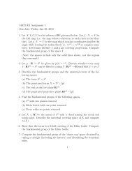
Exercise 1. Consider the 3-sphere S 3 ⊂ R 4 . Using the isomorphism R 4 ∼ = C 2 , we obtain the
inclusion ι : S 3 → C 2 \ {0}. Composing with the projection map π : C 2 \ {0} → CP 1 , we obtain
p = π ◦ ι : S 3 → CP 1 ,
known as the “Hopf fibration”.
Using the coordinate charts given in class for S 3 and CP 1 , compute p in coordinates (one chart
on each of the domain and codomain should suffice). Also, describe explicitly the preimage of a
pair of points in CP 1 under p, using a coordinate chart for S 3 .
Exercise 2. Consider the function f = 1 2 (|x|2 − |y| 2 ) on R p+q , where x = (x 1 , . . . , x p ) and y =
(y 1 , . . . , y q ) together form a standard coordinate system. Describe explicitly all paths of steepest
descent as parametrized curves. Recall that a path of steepest descent is a path γ : R → X which
is an integral curve for the vector field V = −∇f, i.e. it satisfies
Plot these paths for all (p, q) such that p + q = 2.
˙γ = −∇f(γ). (1)
Exercise 3. Let X be the 2-dimensional torus, expressed as R 2 /Γ, where Γ is the translation
action of Z 2 , i.e. (a, b) · (x, y) = (x + a, y + b). In standard coordinates (x, y) for R 2 , consider the
function
h(x, y) = sin 2 (πx) + sin 2 (πy).
i) Determine the critical points of the function h.
ii) Compute the Hessian at each critical point and determine its signature.
iii) Determine and draw the paths of steepest descent as in the exercise above.
iv) Describe how the above responses change when h is replaced with
h(x, y) = sin 2 (2πx) + sin 2 (πy).
Exercise 4. Let X = CP n , with projective coordinates [z 0 : · · · : z n ]. Fix real numbers λ 0 < . . . <
λ n and define the function
∑ n
i=0
f([z 0 : · · · : z n ]) =
λ i|z i |
∑ 2
n
i=0 |z i| . 2
As above, determine the critical points as well as Hessian signatures. Give a qualitiative description
of the paths of steepest descent. Does the above work for real projective space as well? Plot the
paths of steepest descent for RP 2 . It is possible to work on the sphere S 2 using the usual notion
of gradient for functions on S 2 (this uses the usual metric on the sphere).

Differential Topology, Assignment 2 Due date: October 10, 2013
Exercise 5. Recall that Gr(k, V ) is the set of k-dimensional subspaces of the vector space V .
Normally we take V = C n and write Gr(k, n). We will focus on Gr(2, 4) in this exercise. Fix a
basis (e 1 , e 2 , e 3 , e 4 ) for the purpose of defining a full flag F in V , meaning a sequence of subspaces
{0} = F 0 ⊂ F 1 ⊂ F 2 ⊂ F 3 ⊂ F 4 = V,
where F i = Span(e 1 , . . . , e i ). Any point Λ ∈ Gr(2, 4) may then be intersected with the flag, giving
subspaces
Λ ∩ F 1 ⊂ Λ ∩ F 2 ⊂ Λ ∩ F 3 ⊂ Λ. (2)
For most (or an open dense set of, or generic choice of) Λ, the first two subspaces in the above
sequence would be zero, and Λ ∩ F 3 would be 1-dimensional. This set of Λ is called W 0,0 , the
largest “Schubert cell” and is the “usual case”. In general, for special elements Λ ∈ Gr(2, 4), the
1-dimensional intersection in (2) may happen a 1 places earlier than usual, and the 2-dimensional
intersection may happen a 2 places earlier than usual, where a 1 ≥ a 2 . So we may define subsets
W a1 ,a 2
for any such pair (a 1 , a 2 ). For example,
W 1,1 = {Λ ∈ Gr(2, 4) : dim(Λ ∩ F 1 ) = 0 and dim(Λ ∩ F 2 ) = 1 and dim(Λ ∩ F 3 ) = 2.}
i) A point Λ ∈ Gr(2, 4) may be described by giving a spanning pair of vectors for the 2-
dimensional subspace it represents. We express this pair of vectors in terms of the chosen
basis above, and arrange them as the rows of a 2 × 4 matrix
( )
∗ ∗ ∗ ∗
λ =
,
∗ ∗ ∗ ∗
with the understanding that two matrices λ, λ ′ represent the same element of the Grassmannian
when λ = gλ ′ for some g ∈ GL(2, C). Prove that W 1,1 is in bijection with matrices of the
form
( )
∗ 1 0 0
λ =
,
∗ 0 1 0
and obtain analogous statements for the other Schubert cells W a,b , including the largest one.
ii) There is a partial order on the Schubert cells, so that W a,b < W c,d when W a,b is contained in
the closure of W c,d . Determine what the order relation is between the Schubert cells in Gr(2, 4)
and draw the associated Hasse diagram.
iii) By projectivizing C 4 to produce CP 3 , we see that 2-dimensional subspaces Λ ∈ C 4 correspond
to projective lines in the 3-dimensional projective space CP 3 . In this way we see that Gr(2, 4)
may be viewed as the space G(1, 3) of lines in CP 3 . The flag F then becomes a projective
flag, consisting of a choice of point p, projective line l, and projective plane P in CP 3 such
that p ∈ l and l ⊂ P . Give a geometric description of the closure of each of the Schubert
cells in Gr(2, 4), using this projective model.