Master thesis - UBC Physics & Astronomy

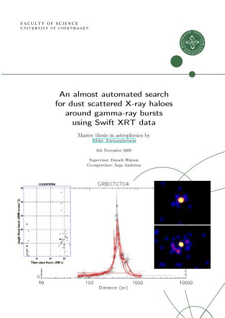
An almost automated search 

for dust scattered X-ray haloes 

around gamma-ray bursts 

using Swift XRT data 

Master thesis in astrophysics by 

Mike Alexandersen 

6th November 2009 

Supervisor: Darach Watson 

Co-supervisor: Anja Andersen

2 M. Alexandersen : Master thesis 

1. Abstract 

In this project, I have investigated methods for discovering and mapping 

dust clouds in our Galaxy. This has been done using the expanding X- 

ray haloes created around the afterglow of some Gamma Ray Bursts 

(GRBs). These haloes occur when X-rays are scattered at small angles 

by dust concentrated in the dust clouds. 

Only five GRB observations have previously been known to exhibit 

these expanding haloes, two of which had two rings, indicating the presence 

of two dust clouds. The most resent four of these GRBs have been 

observed using the Swift, which has detected 477 GRBs to date. The 

Swift XRT observations of these four GRBs are therefore used to develop 

a strategy for reducing and analysing Swift observations of GRB afterglows. 

The aim of this strategy is to detect similar dust scattered X-ray 

haloes in other GRB observations. This strategy was developed into an 

almost automated programme, using a combination of the .fits file manipulation 

software package F T OOLS, the text processing programming 

language P erl and the data analysis programming language IDL. 

Using this programme, Swift observations of 55 GRBs within 10 ◦ of 

the galactic plane, as well as 32 GRBs selected by other criteria, were 

reduced and analysed. This led to the discovery of at least four previously 

unknown dust scattered haloes, in the observations of GRB070704, 

GRB071011, GRB090621a and GRB090807a. From the analysis I found 

that the distances to the dust sheets causing these haloes are ∼ 380 pc, 

∼ 100 pc, ∼ 900 pc and ∼ 81 pc, respectively.

M. Alexandersen : Master thesis 3 

Contents 

1 Abstract 2 

2 Project description 6 

3 Background theory and knowledge 7 

3.1 Gamma-ray bursts . . . . . . . . . . . . . . . . . . . . . . 7 

3.2 Interstellar dust . . . . . . . . . . . . . . . . . . . . . . . . 8 

3.3 Dust scattered X-ray haloes . . . . . . . . . . . . . . . . . 10 

3.3.1 Relationship between distance and time delay . . . 12 

3.4 Scattering of X-rays by dust . . . . . . . . . . . . . . . . . 14 

3.5 Detection of X-rays . . . . . . . . . . . . . . . . . . . . . . 16 

3.6 Swift . . . . . . . . . . . . . . . . . . . . . . . . . . . . . . 20 

4 Previously published dust scattered X-ray haloes 22 

5 Methods of detecting/excluding haloes 23 

5.1 Regular spatial image . . . . . . . . . . . . . . . . . . . . . 23 

5.2 Dynamical image . . . . . . . . . . . . . . . . . . . . . . . 23 

5.3 Dust Distance Distribution . . . . . . . . . . . . . . . . . . 27 

5.4 Fourier transform method . . . . . . . . . . . . . . . . . . 30 

5.5 Convolution method . . . . . . . . . . . . . . . . . . . . . 33 

5.6 Mean/median θ 2 method . . . . . . . . . . . . . . . . . . . 33 

6 Programming 35 

6.1 F T OOLS . . . . . . . . . . . . . . . . . . . . . . . . . . . 36 

6.2 ds9 . . . . . . . . . . . . . . . . . . . . . . . . . . . . . . . 38 

6.3 IDL . . . . . . . . . . . . . . . . . . . . . . . . . . . . . . 39 

6.3.1 SP AW N . . . . . . . . . . . . . . . . . . . . . . . 39 

6.4 P erl . . . . . . . . . . . . . . . . . . . . . . . . . . . . . . 39 

6.5 My IDL procedures . . . . . . . . . . . . . . . . . . . . . 40 

6.5.1 meta . . . . . . . . . . . . . . . . . . . . . . . . . . 40 

6.5.2 object . . . . . . . . . . . . . . . . . . . . . . . . . 41 

6.5.3 ftoolsreducea . . . . . . . . . . . . . . . . . . . . . 43 

6.5.4 blacknwhite . . . . . . . . . . . . . . . . . . . . . . 47 

6.5.5 grbnameauto . . . . . . . . . . . . . . . . . . . . . 49 

6.5.6 main . . . . . . . . . . . . . . . . . . . . . . . . . . 50 

6.5.7 ftoolsreduceb . . . . . . . . . . . . . . . . . . . . . 51 

6.5.8 loglogmere . . . . . . . . . . . . . . . . . . . . . . 54 

6.5.9 loglogmerebaggrund . . . . . . . . . . . . . . . . . 60 

6.5.10 fitcurves . . . . . . . . . . . . . . . . . . . . . . . 64 

6.5.11 meantheta2 . . . . . . . . . . . . . . . . . . . . . . 72


7 Testing and final debugging 77 

7.1 Testing starting boundaries . . . . . . . . . . . . . . . . . 81 

7.1.1 Final boundaries . . . . . . . . . . . . . . . . . . . 86 

7.2 Final test . . . . . . . . . . . . . . . . . . . . . . . . . . . 87 

7.2.1 The DDD results . . . . . . . . . . . . . . . . . . . 87 

7.2.2 The mean/median θ 2 branch . . . . . . . . . . . . . 89 

7.3 Important plots . . . . . . . . . . . . . . . . . . . . . . . . 91 

8 Results 96 

8.1 Final results . . . . . . . . . . . . . . . . . . . . . . . . . . 97 

9 Discussion and possible extensions of this work 118 

9.1 The data used . . . . . . . . . . . . . . . . . . . . . . . . . 118 

9.2 The mean θ 2 method . . . . . . . . . . . . . . . . . . . . . 119 

9.3 Background subtraction . . . . . . . . . . . . . . . . . . . 122 

9.4 User interaction with programme . . . . . . . . . . . . . . 124 

9.5 Energy range used . . . . . . . . . . . . . . . . . . . . . . 124 

9.6 Integrated counts . . . . . . . . . . . . . . . . . . . . . . . 125 

9.7 Point spread function . . . . . . . . . . . . . . . . . . . . . 126 

9.8 Use of ds9 . . . . . . . . . . . . . . . . . . . . . . . . . . . 126 

9.9 Results . . . . . . . . . . . . . . . . . . . . . . . . . . . . . 127 

9.9.1 Comparison with literature . . . . . . . . . . . . . . 128 

9.9.2 New haloes discovered . . . . . . . . . . . . . . . . 129 

10 Conclusion 131 

11 Bibliography 133 

12 Acknowledgements 135 

A Abbreviations 136 

B The illusion 137 

C Downloading data from the Swift archive 138 

D Examples of output data files 150 

D.1 GRB070129fitparams.txt . . . . . . . . . . . . . . . . . . . 150 

D.2 GRB070129bestpeak.txt . . . . . . . . . . . . . . . . . . . 153 

D.3 GRB070129meandata.txt . . . . . . . . . . . . . . . . . . . 154 

E Information about the data downloaded from the Swift 

archive 156 

F Results: SN vs. distance plots 158


G My IDL code 167 

G.1 meta . . . . . . . . . . . . . . . . . . . . . . . . . . . . . . 167 

G.2 object . . . . . . . . . . . . . . . . . . . . . . . . . . . . . 168 

G.3 ftoolsreducea . . . . . . . . . . . . . . . . . . . . . . . . . 169 

G.4 blacknwhite . . . . . . . . . . . . . . . . . . . . . . . . . . 172 

G.5 grbnameauto . . . . . . . . . . . . . . . . . . . . . . . . . 172 

G.6 main . . . . . . . . . . . . . . . . . . . . . . . . . . . . . . 173 

G.7 ftoolsreduceb . . . . . . . . . . . . . . . . . . . . . . . . . 176 

G.8 loglogmere . . . . . . . . . . . . . . . . . . . . . . . . . . 181 

G.9 loglogmerebaggrund . . . . . . . . . . . . . . . . . . . . . 184 

G.10 fitcurves . . . . . . . . . . . . . . . . . . . . . . . . . . . 195 

G.10.1 lorentz1 . . . . . . . . . . . . . . . . . . . . . . . . 210 

G.10.2 lorentz2 . . . . . . . . . . . . . . . . . . . . . . . . 210 

G.10.3 lorentz2 . . . . . . . . . . . . . . . . . . . . . . . . 210 

G.10.4 constantlorentz1 . . . . . . . . . . . . . . . . . . . 211 



G.10.7 power . . . . . . . . . . . . . . . . . . . . . . . . . 212 

G.10.8 powerlorentz1 . . . . . . . . . . . . . . . . . . . . . 212 

G.10.9 powerlorentz2 . . . . . . . . . . . . . . . . . . . . . 213 

G.10.10powerlorentz3 . . . . . . . . . . . . . . . . . . . . . 213 

G.11 meantheta2 . . . . . . . . . . . . . . . . . . . . . . . . . . 213


2. Project description 

The scattering of X-rays provides information about the distribution of 

dust and its properties. Using scattered X-rays from Gamma Ray Bursts 

(GRBs) I will investigate the distribution and properties of dust in the 

Galaxy. X-ray data from the Swift mission will be used. 

The Swift satellite is a space observatory with its main focus on GRBs. 

It is therefore designed to quickly detect a GRB on the sky, and rapidly 

rotate to its position and start observing. Swift has several instruments 

on board, and can therefore observe GRBs and their afterglow not only in 

gamma ray wavelengths, but promptly in X-rays, allowing many GRBs 

to be observed while still bright, providing a data set suitable for this 

study. 

When the X-rays come from GRBs, it is a short burst and not a continuous 

source. Because of this, one first observes X-rays that have travelled 

directly from the source to the observer, followed by an expanding 

halo around the source of X-rays that would otherwise have missed the 

observer, but has been scattered by dust into the observer’s direction. 

The reason for the time dependence is the larger travel distance from 

source to observer for the scattered light. 

The goal of this project is to design a strategy for searching for these 

haloes. The Swift observations within 10 ◦ of the galactic plane will be 

analysed using this strategy. This will hopefully lead to the discovery of 

previously unknown dust-scattered X-ray haloes in a few of the ∼ 80 

GRB observations that will be analysed. This has never previously been 

done, and only five GRBs have previously been known to exhibit a dust 

scattered halo. Finding new dust clouds helps further our understanding 

of the evolution of our Galaxy.


3. Background theory and knowledge 

3.1. Gamma-ray bursts 

Gamma-ray bursts (GRBs 1 ) are the most energetic explosions in the 

known Universe. They are seen as bright, short bursts, with most of the 

energy radiated in γ-rays, hence their name. They span several orders of 

magnitude in duration, with the time for 90% of the total energy output of 

the burst to be emitted ranging from less than 0.01 s to more than 100 s 

(Piran 2004). Bursts are grouped in two classifications, short duration 

bursts lasting less than 2 s, and long duration bursts lasting longer than 

2 s. 

It was once believed that GRBs radiate isotropically, thereby giving 

them luminosities of the order 10 17 − 10 18 L⊙ ≈ 10 44 − 10 45 W. However, 

it has since been discovered that most of the GRB energy is emitted along 

narrow jets, meaning that their total luminosities are "only" of the order 

10 17 L⊙ (Piran 2004). This is still a huge amount of power, but because 

GRBs are much shorter in duration than supernovae, the total energy 

released in the two forms of giant explosions are similar. 

As this large amount of energy is emitted along narrow jets, the energy 

densities in these jets are very high. GRBs can therefore be seen from 

some of the furthest parts of the observable Universe, allowing us to study 

the early Universe at just a fraction of its current age (Hjorth et al. 2005). 

Little is known about short duration bursts, and long duration bursts 

are still not fully understood. The currently accepted theories for GRBs 

tell us that the main burst is produced when the core of an ultra high 

mass star collapses (long duration bursts), or when two neutron stars 

merge (short duration bursts). When this happens, two jets of highly 

energetic particles travelling at near the speed of light is emitted from 

the core along its rotation axis. Far outside the surface of the original star, 

particles in the jet travelling at slightly different speeds start colliding, 

thereby emitting the flash of γ-rays seen as the GRB (Hjorth et al. 2005). 

GRBs are usually followed by longer afterglows in less energetic radiation. 

This afterglow comes from the interstellar medium surrounding 

1 The most common abbreviations used in this thesis is presented in Tab. A.1


the burst, which gets shock heated as the jets plough through and collide 

with it (Piran 2004). 

GRBs are seen in random directions in the sky, as they do not occur 

in our Galaxy, but much further away, on cosmological distances. From 

observations of the afterglows, it has been possible to identify the host 

galaxy of many GRBs. It is seen that GRBs occur in star forming galaxies, 

so places where it is possible to find the short lived, super massive 

stars that it is believed to be the origin of long duration GRBs. This 

is also supported by the fact that we do not see GRBs in our own or 

neighbouring galaxies, as the high metallicity prevents these high mass 

stars from forming. GRBs therefore predominantly happen in the early 

Universe, in metal poor galaxies (Piran 2004; van Paradijs et al. 2000). 

3.2. Interstellar dust 

Interstellar dust is small solid particles covering a range of sizes from 

about hundred molecules up to a few µm. The dust contributes only a 

small fraction of the mass of the Galaxy, but occupy a large part of its 

volume. Although the interstellar medium in most places have very low 

densities, over large distances the dust can have a significant effect on 

light from other objects. 

Dust absorbs and scatters visible light, thereby darkening observations 

of objects behind the dust. The efficiency of absorption and scattering, 

collectively known as extinction, is greater for higher energies, so blue 

light is extinguished more than red light, causing the object to also appear 

redder than it really is. The absorbed radiation heats the dust, which then 

emits black body radiation, dominantly infrared radiation, thereby also 

obscuring observations in these wavelengths. 

Extinction by dust has been known as a problem in astronomy since 

the early 20 th century. The effects of dust in our Galaxy can be seen 

with the naked eye on a clear, moonless night. Fig. 1 shows a photograph 

of the Milky Way, over Devils Peak, Wyoming. Unobscured, the galaxy 

should be seen as a big bright band across the sky, but we clearly see 

a lot of darker streaks and patches. These areas are dark because dust 

within our Galaxy extinguish the light on its way to us.


Figure 1. The Milky Way Galaxy, seen over Devils Tower, Wyoming. 

The dark areas along the Milky Way are caused by dust extinction. Photo 

form APOD (2009). 

Other galaxies, when seen edge on, show very similar dust patterns as 

we see in the Milky Way, whereas for galaxies seen away from edge on, 

far less dust extinction is seen. This confirms that the interstellar dust is 

concentrated in a thin disk, as the stars of the galaxy are. The dust in the 

Galaxy is believed to be predominantly in disk with thickness ∼ 200 pc 

(Whittet 1992). 

For many years, interstellar dust was studied exclusively to obtain 

knowledge of position and density of the dust, so that observations of 

other objects behind the dust could be corrected for the extinction effects. 

This is still an important field of research, but in resent years, the 

interstellar dust has gained interest in itself. Dust has been discovered to 

be an important component of the evolution of galaxies. Interstellar dust 

is believed to possibly acts as a catalyser in the gravitational collapse 

of protostars, and the subsequent collapse of the circumstellar disk into 

planets (Whittet 1992). These events take place in areas with higher than 

average density of interstellar dust and gas. 

For dust to form, the particle density must be high, so that the probability 

of particles colliding is also high. This means that the interstellar 

dust cannot have formed in its current location, as the interstellar environment 

has a particle density of ∼ 10 6 m −3 (Whittet 1992). This is


10 19 times less than the Earths atmosphere at sea level. The temperature 

must also be low enough so that the particles combine when colliding, 

rather than breaking each other up. Dust is therefore believed to be created 

in the outflow and mass loss of stars nearing the end of their life 

span. These outflows have just the right conditions needed for dust to 

form. As the particle-flow moves outwards, it cools down. At some point, 

while the density of the flow is still high, the temperature will have fallen 

sufficiently to allow dust formation. 

This ejection of dust and gas to the interstellar medium enriches the 

medium with heavy elements. This causes the galaxy to have scattered 

patches of higher dust density, known as dust clouds or nebulae. The enriched 

interstellar medium can in turn condense and collapse to form new 

stellar systems. The heavy elements allows for the formation of planetary 

systems and are also vital for the formation of biology. Studying the dust 

in the interstellar medium therefore improves our knowledge and understanding 

of galaxy evolution, star formation and death, planet formation 

and life in the Galaxy. 

3.3. Dust scattered X-ray haloes 

The dust in the interstellar medium will scatter radiation from the GRB. 

This is most prominently seen if a cloud of dust happens to lie in our line 

of sight to a GRB. This scattering is most effective in X-ray energies, see 

Sec. 3.4. Most X-rays are not scattered, though, so we observe a bright 

point source at the position of the GRB. 

X-rays that travel from the source in a small angle relative to the line 

from us to the GRB, would normally not be observed, but because of the 

dust cloud, a fraction of these X-rays will get scattered into a new path 

that hits us, as seen in Fig. 3. These scattered photons will be observed 

as coming from a different direction in the sky than the source location. 

We observe this as X-rays at small angles, θ, from the position of the 

source. For a constant source, this would create a halo from the point 

source and out, fading with the angle from the source, but constant in 

time.


Figure 2. This is the XMM observation of GRB031203, split into time 

intervals, clearly showing the presence of an expanding halo, and faintly 

revealing that there are two rings, caused by dust sheets at two separate 

distances. Each frame covers a time interval of 5780 s, after the beginning 

of observation, 22081 s after the burst. The data has been filtered to the 

0.7 − 2.5 keV energy interval. S2 and S3 are foreground sources, S1 is the 

GRB afterglow. This image is taken from Vaughan et al. (2004) 

Because the path of a photon from the GRB to us is longer for larger 

scattering angles, the time it takes to travel this distance is of course 

also larger (t = d/c). This means that photons leaving the source at the 

same time, would be observed on Earth at different times, dependant on 

their scattered angle. For a constant source, this time delay would not be 

observable, but due to the fact that a GRB is a rather short event in time, 

this time delay is very noticeable, and a useful observable feature. Since 

the GRB is an almost instantaneous event, all photons from it are emitted 

almost simultaneously. Therefore, for any very short period in time, only 

a thin interval of scattering angles should be observed, as larger angles 

have not arrived yet, and smaller angles have already arrived previously. 

At a later time, a similar interval of larger scattering angles would be 

seen, as seen in Fig. 2.


The X-ray afterglow of the GRB actually lasts slightly longer than the 

actual burst. However, it begins already during the GRB, and most of 

the emitted X-rays are radiated during the early part of the afterglow, so 

the X-rays can still be seen as being emitted almost instantaneously, and 

at the time of the burst. Therefore, on the CCD detector in the camera, 

or on the sky if that was possible, one first sees a very bright point source 

appear and start to fade away, followed by a much dimmer halo centred 

on the point source, starting close to the GRB position, expanding to 

larger angles with time. 

3.3.1. Relationship between distance and time delay 

The size of the halo at a given time can be used to determine the distance 

from the observer to the scattering layer of dust, as the time delay is related 

to the scattering angle and the distance travelled. This relationship 

is derived below. 

See Fig. 3 for a diagram of the angle and distances used in this derivation. 

D s = the distance from the observer to the source, along the line of sight. 

D d = the distance from the observer to the dust, along the line of sight 

to the source. 

D ds = D s − D d = the distance from the dust to the source, along the line 

of sight from the observer to the source. 

h d = the distance from the observer to the point of scattering in the dust 

cloud. 

h ds = the distance from the source to the point of scattering in the dust 

cloud. 

θ = the observed angle between the source and the scattering. 

c = the speed of light. 

t = the observed time delay between arrival of scattered and un-scattered 

photons. 

We know that the distance travelled is equal to the speed multiplied 

with the time travelled. The photons travelling along the scattered path 

can clearly be seen from Fig. 3 to travel further than the un-scattered 

photons. As the photons all travel at the speed of light, the difference in


Figure 3. The X-rays from the source is scattered by the dust at the 

small angle θ, thereby being observed as a halo around the source. The 

scattering angle is greatly exaggerated in this diagram, for clarity. The 

broken lines going to the source indicate that these distances are much 

longer than the other distances in the diagram, and resultantly are virtually 

parallel. 

distance is proportional to the difference in travel time: 

h d + h ds − D s = ct. (1) 

From the geometry of Fig. 3 it is clear that 

h d = D d 

(2) 

√ 

cos θ 

h d s = Dd 2 tan2 θ + Dds 2 . (3) 

The distance to the dust is much smaller than the distance to the source, 

and θ ≪ 1, so collectively D d tan θ ≪ D ds , so 

h ds ≃ D ds . (4) 

Using Eq. (1), (2), (4) and the fact that D ds = D s − D d we can derive 

D d 

cos θ + D ds − D s = ct, (5) 

D d 

cos θ − D d = ct, (6) 

D d (1 − cos θ) 

cos θ 

D d = 

= ct, (7) 

ct cos θ 

1 − cos θ . (8)


As mentioned earlier θ ≪ 1, so cos θ ≃ 1 − 1 2 θ2 . From this, Eq. (8) 

becomes 

D d = ct ( 1 − 1 2 θ2) 

1 

2 θ2 . (9) 

With θ ≪ 1 we now apply that 1 − 1 2 θ2 ≃ 1, so finally we get 

D d = 2ct 

θ 2 . (10) 

Writing this in typical units for dust scattered X-ray haloes, the above 

equation becomes 

D d ≃ 827 pc t 1 arcsec 2 

. (11) 

1 s θ 2 

As h ds ≃ D ds , the X-rays hitting the dust are moving almost parallel 

to each other. Therefore θ ≃ the scattering angle, and will be referred to 

as the scattering angle in this thesis. 

3.4. Scattering of X-rays by dust 

In order to see this kind of halo, the dominant scattering process must be 

small angle scattering and not Rayleigh scattering or other physical processes. 

For Rayleigh scattering light is scattered in all directions, whereas 

small angle scattering only scatters radiation within a fairly small interval 

of angles, in the forward direction. Rayleigh scattering applies when 

the wavelength of the radiation is larger than or similar to the scattering 

particles (Whittet 1992). In the case of interstellar dust of typical 

size 0.2 µm (Vaughan et al. 2004), in order for the wavelength to be 

much smaller than the dust size, thereby making small angle scattering 

the dominant process, the radiation has to be γ-rays, X-rays or the 

high energy end of Ultra Violet (UV). The upper boundary on the X- 

ray wavelength is 10 nm, which safely satisfies the condition that the 

wavelength should be much smaller than the dust grain. 

Small angle scattering depends on the principle of total internal reflection. 

When radiation hits a surface between two media at an angle of


Figure 4. The angle of incidence, θ i , transmission, θ t , reflection, θ r and 

the critical angle, θ c , are all defined relative to the normal to the surface. 

Medium 1, with refractive index n 1 is the medium in which the incident 

and reflected radiation travel. Medium 2, with radiative index n 2 is the 

medium where the transmitted radiation travel. If θ i < θ c , light is both 

transmitted and reflected (left), but if θ i ≥ θ c then all the radiation is 

reflected (right) 

incidence θ i , part of it will be reflected at angle θ r = θ i , and part will be 

transmitted at angle θ t . The fraction of the radiation that is reflected and 

transmitted depends on θ i and the index of refraction of the two media. 

How much radiation is reflected and transmitted will not be explained in 

detail here, for further information see Fowles (1990). However, above a 

certain critical angle, θ c , the transmitted fraction drops to zero and total 

internal reflection occurs. This angle is defined in Guenther (1990) by 

( ) 

n2 

θ c = arcsin , (12) 

n 1 

where n 1 and n 2 are the refractive indices of medium 1 and 2 respectively, 

as seen in Fig. 4. So for incidence angles larger than θ c all of the radiation 

gets reflected. The existence of a critical angle of course requires that 

n 2 

≤ n 1 . In the case of interstellar dust, medium 1 is the vacuum of 

space, so n 1 = 1 at all wavelengths, and medium 2 is the dust grain. 

For most materials, the refractive index n is greater than unity at most 

wavelengths, thereby not fulfilling the above requirement. However, as 

can be seen from Fig. 5, for X-ray energies, and a few other smaller ranges, 

n is in fact less than unity, thereby allowing total internal reflection on


Figure 5. A rough graph showing the dependance of the refractive index 

on radiation energy. Besides the general shape depicted, some dips exist 

near absorption resonances. This graph has been adapted from Attwood 

(2007). 

the outside of a material surrounded by vacuum. This is another reason 

why we only see this effect at X-ray energies. 

As can be seen from Fig. 5, the refractive index goes asymptotically 

towards unity as the energy of X-rays increase. Using Eq. (12) it is clear 

that as n 2 /n 1 → 1, θ c → 90 ◦ . So, since higher energies have n 2 closer 

to unity, the critical angle for total internal reflection gets so large, that 

the interval of angles available for total reflection (θ c to 90 ◦ ) decreases. 

Going back to the problem at hand, this therefore means that at higher 

energies, the radiation is increasingly unlikely to hit the dust particles at 

an incident angle that allows total internal reflection, and thereby small 

angle scattering 2 . 

3.5. Detection of X-rays 

X-ray observation is in no way similar to or as easy as optical observation. 

First of all, celestial X-rays can only be observed from space. This 

means that in order to observe X-rays we have to build large satellites, 

2 So the "small angles" needed gets smaller and smaller for increasing energy. 

It is a confusing convention that θ i is measured relative to the normal to the 

surface, so that θ i has to be large to allow small angle scattering.


Figure 6. A medical X-ray 

image of the insides of an unlucky 

patient. 

which of course is far more expensive than telescopes built for ground 

based use. 

We know X-rays from the medical uses in photographing our bones. 

This works because X-rays are highly energetic, so they do not get reflected 

or absorbed by our flesh, and easily pass through us, unlike visible 

light. However, they do not pass through denser materials like bones, 

implants and forks, see Fig. 6. 

The molecules in the Earths atmosphere do not absorb visible light 

apart from in a few absorption lines, where the energy of the light photon 

allows a jump from one energy level to another within the molecule. 

However, X-rays are energetic enough that if they hit something, the 

energy transferred to the molecule is enough to release an electron from 

the molecule. Since this process does not have one distinct energy like a 

jump in energy level does, but only has a minimum energy (the ionisation 

energy), the whole continuum of X-ray energies gets absorbed in the 

atmosphere. This does not happen very efficiently, otherwise they would 

also get absorbed in our body when the doctor takes an X-ray image of 

us. However, the atmosphere is roughly 100 − 120 km thick, so X-rays 

travelling through the atmosphere would encounter as many molecules 

as in 5 m layer of concrete, effectively stopping all X-rays from reaching 

the surface of the Earth (SOA 2009).


Another thing that makes X-ray observation difficult and expensive is 

the fact that regular telescope designs, as known from optical telescopes, 

cannot be used. Normal telescope designs rely on reflection off mirrors at 

an incidence angle close to the normal of the surface to focus the beam of 

light. However, X-ray photons have so high energies, that they do not get 

reflected at these angles and will pass straight through the mirror. This 

is because for all reflection, the photon must be considered to be a wave. 

When a wave hits a change in refractive index (so, a surface), part of 

the wave is reflected, and part of it is transmitted at a slightly deflected 

angle. How much of the wave is transmitted and reflected depends on 

the energy of the wave, and the incoming angle. For higher the energy, a 

larger fraction of the wave is transmitted through the surface. 

At a critical angle, θ c , the transmitted fraction drops to 0, and total 

internal reflection occurs. This critical angle depends on the ratio of the 

refractive index of the two media, here vacuum and the mirror, which 

again depends on the energy of the radiation, see Fig. 5. This means that 

the critical angle for X-rays is high, but it is possible to reflect them using 

gracing incidence angles. 

This is then the process used in X-ray telescopes, as can be seen in 

Fig. 7. A large mirror tube following a paraboloid shape first reflects the 

X-rays once, focusing them towards the focal point of the paraboloid. As 

the distance to this focal point from the part of the paraboloid where 

the slope of the mirror is small enough to allow total internal reflection 

is still very large, yet another tubular mirror is used. This mirror is in a 

hyperboloid shape. Finally, the beam has been focused to the focal point 

of the hyperboloid mirror. However, this is still quite far from the point 

of reflection, so typical X-ray telescopes have a focal length of 5 − 10 m. 

The combination of a paraboloid and hyperboloid mirror, called a 

Wolter type 1 design, is used because this design creates a perfect image 

for on-axis objects. However, as described in Conconi & Campana (2001), 

aberrations increase rapidly for off-axis angles. It is therefore always best 

to have the object of interest as close as possible to the centre of the field 

of view.


Figure 7. A view of the mirror structures used for most X-ray telescopes, 

called the Wolter type I design. Incident X-rays are reflected off the 

paraboloid surface, then the hyperboloid, both at grazing angles, into 

the focus of the hyperboloid. The angles are exaggerated for illustration 

purposes, and the structure is actually much longer than its radius. 

Illustration from ESA (2009a). 

Figure 8. A side view of 

how many mirror tubes can 

be nested inside each other, 

to increase the area covered. 

Illustration from NASA 

(2008). 

The mirror design does not cover a very large area perpendicular to 

the beam of photons, compared to the radius of the tubes. However, due 

to the tubular shape, it is possible to place many tubes inside each other, 

thereby increasing the collecting area of the telescope, see Fig. 8. 

A CCD camera is placed in the focal plane. Because X-ray sources are 

fairly dim, and the photons have high energies, it is possible to count 

single photons using the CCD. The charges on the CCD is read out at 

a time interval short enough to minimise the probability of two photons


hitting the same pixel in the same time interval. Therefore, all charge in 

a CCD pixel is due to one photon, and the amount of charge is proportional 

to the photon energy, so the energy of each pixel can be found. 

This means that X-ray observations contain more information than ordinary 

observations do. Besides the two-dimensional image that ordinary 

observations give us, X-ray observation adds a third, time, dimension, 

and allows spectroscopy and imaging to be made from the same observation 

using the same instrument. Finally, because every single photon is 

identified with its own position, time, and energy, it is possible to see if 

a certain area of the image has a different spectrum than the rest, or to 

see changes in time. 

3.6. Swift 

The Swift satellite is a space observatory dedicated for GRB observation. 

It is equipped with a large γ-ray detector, the Burst Alert Telescope 

(BAT), which covers roughly one sixth of the sky at any time. When this 

detector registers a burst, the position is calculated, and the telescope 

swiftly and automatically turns to point directly to this position. This 

allows two other instruments, with much smaller fields of view, to observe 

the afterglow of the GRB. These are the small X-Ray Telescope (XRT) 

and the UltraViolet/Optical Telescope (UVOT). 

Swift has been placed in a low altitude orbit, with an orbital period 

of roughly 90 min = 5400 s. Here, the Earths magnetic field ensures that 

Swift is shielded from most of the high energetic particles emitted from 

the Sun during solar flares. This means that Swift can be light and not 

carry much onboard shielding, allowing it to turn from one position in 

the sky to another within 75 s, using far less power than if it had heavy 

shielding. The short orbital period, however, also means that continuous 

observation of a source is not possibly for long durations, as the continuity 

will be broken each time Swift moves behind the Earth. However, 

if observations are made over several orbits, useful data can still be obtained. 

For this thesis, data from the Swift XRT will be used. An example of 

how to download Swift data from the public archive can be seen in App.


C. XRT data are provided in event files in the fits format commonly 

used in astronomy. An event file is a file which contains a table with one 

row for each observed photon, known as an event. The table contains the 

x and y position on the CCD that the photon hit, the time of detection 

and the energy measured for the photon, as well as a few other properties 

of each event. The fits file also contains a header, which contains more 

general information on the observation, such as the co-ordinates on the 

sky that the telescope is pointed at, and any settings of the detector that 

may be relevant. If the observation was triggered by a BAT detection, 

the header will also contain a keyword specifying the time of the burst.


4. Previously published dust scattered X-ray 

haloes 

There is, to my knowledge, only five GRBs known from literature to have 

expanding dust scattered X-ray haloes, see Tab. 1. 

The first ever observed GRB with a halo (two haloes in fact), 

GRB031203, happened more than two years before Swift came into operation, 

so only XMM-Newton data exists for this burst. It has therefore 

not been included in my final analysis, which only involve Swift observations. 

However, as it is the best data, and the most previously analysed, 

I used it as a prototype in the beginning of this work. I reduced it and 

reproduced diagrams similar to those in Tiengo & Mereghetti (2006), in 

order to develop and verify my methods. 

The halo around GRB050713a has only been published using XMM 

data in Tiengo & Mereghetti (2006), and here it is only just distinguishable, 

so it may well be too faint to see using Swift data. I will, however, 

attempt to optimise my analysis methods, so that the halo in even this 

Swift data can be found, without showing false signs of a halo in data 

that does not have a halo. 

The haloes around the last three GRBs in Tab. 1 have all been published 

using Swift data, and should therefore easily be seen from my 

analysis, so I will use these three during development of my analysis 

strategy. 

Table 1. The five GRBs with published haloes. 

Name Literature references Halo(es) seen, caused by lii bii 

dust cloud(s) at (pc) 

GRB031203 Vaughan et al. (2004), 882. ± 20. 255.73 −4.80 

1388. ± 32. 

Watson et al. (2006), 868. +17. 

−16. 

1395. +15 

−30 

Tiengo & Mereghetti (2006) 870. ± 5. 

1384. ± 9. 

GRB050713a Tiengo & Mereghetti (2006) 364. ± 6. 112.15 18.83 

GRB050724 Romano et al. (2005) 175. ± 50. 

Vaughan et al. (2006) 139. ± 9. 350.37 15.10 

GRB061019 Vianello et al. (2007) 940. ± 40. 181.74 4.25 

GRB070129 Vianello et al. (2007) ∼ 150. 157.20 −44.66 

∼ 290.


5. Methods of detecting/excluding haloes 

5.1. Regular spatial image 

For a bright halo, and with good data, such as the XMM observation of 

GRB031203, the halo can easily be seen, even when cut into several time 

intervals, as in Fig. 2. 

For Swift observations this can be difficult, due to the significantly 

smaller count rate. However, if filtered in the best energy range and 

binned to bring out the details, a halo can be vaguely seen, as for example 

in Fig. 9. 

However, this method has many disadvantages. First of all, it can be 

difficult to see a slight over abundance in counts with the naked eye. 

Our eyes have a tendency to not work as well quantitatively as we might 

think. To prove this point, see the illusion in Fig. 10. 

The events are spread out over three dimensions, two spatial dimensions 

and time. When there is, as in most reduced Swift observations, 

only a few hundred to thousand counts, this means there is quite far 

between them. When looking at a regular image we only see the two spatial 

dimensions, and not the time. This means that we cannot see that 

the ring is expanding, and because all times are included, the rings at 

different times will overlap, simply causing a blur around the GRB. 

To see that the ring is actually expanding, the data needs to be split 

into time intervals, so that an image from each time interval can be 

made, and one can see that the ring expands from one image to the next. 

This of course requires a lot of counts, since the more time intervals the 

observation is cut into, the fewer counts there are per image, making the 

ring more difficult to see. 

5.2. Dynamical image 

Tiengo & Mereghetti (2006) and Vianello et al. (2007) both use dynamical 

images to illustrate the presence of an expanding halo around GRBs. The 

dynamical image of GRB031203 can be seen in Fig. 11.


Figure 9. The Swift observation of GRB050724, split into time intervals 

to clearly show the expanding halo. From top left to bottom right: 345 − 

1000 s after the burst, 1000 − 2322 s after burst, 6068 − 8120 s after burst 

(entire second orbit), 11990 − 13881 s after burst (entire third orbit). All 

the data has been filtered to the 0.8 − 2.2 keV energy range. The halo is 

clearly visible in both parts of the first orbit, and is clearly expanding. 

In the second orbit, the ring is visible at a larger radius, and in the third 

orbit the halo is still faintly visible. 

A dynamical image effectively reduces the original three-dimensional 

image to a two dimensional one. The two spatial dimensions are combined 

into one, the angle out from the GRB position, θ. Since the haloes are 

circular on the ordinary image, all parts of a ring is at the same angle 

from the GRB position, so at a given time, an entire ring in the ordinary 

image is represented by a single point in the dynamical image, thereby 

combining all the counts and making it significantly more visible relative 

to the background.


Figure 10. Are tiles A and B the same colour? Yes, they are, see Fig. 

B.1 if in doubt. Our eyes see what they want to see, and in the same 

way it can be difficult to see an over density of points. Illustration from 

APOD (2009). 

In a dynamical image, the angle is usually plotted as the angle squared, 

θ 2 , since, as seen in Eq. (11), when time is plotted on the x-axis and θ 2 on 

the y-axis, a dust scattered X-ray halo should then show up as a straight 

line. The slope of this line, from rearranging and differentiating Eq. (11), 

will be 

dθ 2 

dt 

= 827 

arcsec2 

s 

1 pc 

D . (13) 

However, there is another advantage of doing this, which I will come back 

to. 

In the spatial image, the counts are in a natural binning; the pixel size 

of the CCD. When θ 2 is calculated from spatial co-ordinates, this binning 

is lost, because it is impossible to draw perfect circles in a squared grid. 

The many different combinations of x and y co-ordinates will lead to a 

set of θ 2 values that contain more different numbers than x or y does. 

If one was to simply use the largest common divisor of these θ 2 values, 

one would get a huge image, which would be mainly empty, with a few 

counts here and there.


Figure 11. The dynamical image of GRB031203, from Tiengo & 

Mereghetti (2006). The expanding rings (here straight lines) are clearly 

visible across the entire observation. 

The time resolution of Swift data gives time steps too small to simply 

plot on the x-axis of the dynamical image. So both θ 2 and the time needs 

to be binned. How large the bins need to be depends on the data, and 

on the slope in Eq. (13). This is because a steep line may be more visible 

if the bins in θ 2 are large, whereas for a shallow slope, for the halo to 

not blend in with the afterglow at the bottom of the dynamical image, 

the θ 2 bins will need to be smaller. For an XMM data set like the one of 

GRB031203 that I experimented a bit with, a binning of 3000 s in time 

and 2000 arcsec 2 in θ 2 was well suited for making a dynamical image 

where the presence of two expanding rings is clearly visible, as seen in 

Fig. 11. 

The other advantage of using θ 2 on the y-axis of the dynamical image is 

that this makes the background have the same level all over the image. If 

one imagines a bin in angle as an annulus centred on the GRB position in


Figure 12. This diagram shows the clear difference between binning θ 

or θ 2 . Left shows bins in θ, right shows bins in θ 2 . θ bins cover a larger 

area at larger radius, whereas θ 2 bins cover a constant area. 

the spatial image, this bin covers a certain amount of pixels. If the annulus 

is then stretched to a larger radius, but still has the same thickness, it will 

cover more pixels, and the count in this bin would inevitably be higher 

than in the first bin, because more background is seen by the last bin. 

This would be binning θ, and making a dynamical image with just θ on 

the y-axis would have low counts at the bottom, and then get brighter 

towards larger angles. 

However, if one bins θ 2 , the expansion of the annulus radius happens 

along with the width of the annulus getting smaller. The effect is that 

all the bins cover the same amount of pixels, and should therefore pick 

up the same amount of background noise. The difference in binning in θ 

or θ 2 can be seen in Fig. 12. When plotting a dynamical image with θ 2 

on the y-axis, a uniform background in the spatial image should also be 

seen as a uniform background in the dynamical image. 

My procedure ftoolsreduceb, see Sec. 6.5.7, makes a few dynamical 

images, with different bin sizes, so that the halo might be seen. 

5.3. Dust Distance Distribution 

The Dust Distance Distribution (DDD) is a method used in Tiengo & 

Mereghetti (2006) and Vianello et al. (2007). One assumes that all the 

observed events are caused by X-rays from the GRB, scattered on their


Figure 13. The DDD for the XMM PN observation of GRB031203, 

binned in bins of 20 pc, using fplot. It is clear that this form of binning 

cannot be good across the entire range in distances. 

way to Earth. The distance to the point of scattering, D i , for each event, 

can then be calculated using equation Eq. (11) rewritten as 

D i = 827 pc t i 

1 s 

1 arcsec 2 

, (14) 

where t i is the time since burst, and θ i is the scattering angle (the angle 

between the source GRB and the event, on the sky). 

These distances are then binned into bins of equal number of counts, 

rather than equal widths. This is done because the distances span over 

several orders of magnitude, from 10 1 pc to 10 4 pc. Constant bin size 

would give very few bins with a lot of counts at low distances, and very 

many bins, most of which would be empty, at high distances, as for example 

in Fig. 13. Binning instead with a constant number of counts in 

θ 2 i


Figure 14. The DDD for the XMM PN observation of GRB031203, 

binned with 100 counts in each bin. This graph is taken from Tiengo 

& Mereghetti (2006) 

each bin gives us a good resolution over the whole range. This binning 

therefore allows us to plot the DDD, with the distance to the supposed 

scattering on the x-axis and the density of counts on the y-axis, on logarithmic 

axes, as in Fig. 14 

A lot of counts will in fact be background, and not actual scattering 

photons from the GRB. These background counts will cause a background 

in the DDD, which follows a power law over most of the distances, with 

a power law index of −2. At low distances, the background will be lower 

than the power law, as also seen in Fig. 13. This is because events giving 

these low distances, need large θ i values, or small t i values. At some 

time, the large θ needed for a low distance will move off the edge of the 

CCD, and therefore the longer the time interval observed, the larger is 

the distance at which the background starts following the −2 power law. 

If there is a scattering dust sheet, it will show up as a peak on top of 

the background curve. A Lorentz distribution can be fitted on this peak, 

and the distance of the dust sheet can thereby be found. The reason 

this is a Lorentz distribution is that even though the dust cloud may 

only be a thin sheet, the cameras point spread function (PSF) causes the


distribution to be spread out. In most cases, most of the width of the 

Lorentz peak is due to the PSF, and not due to the thickness of the dust 

sheets. Unless the peak is significantly wider than the width caused by 

the PSF, little information is therefore available about the dust sheets 

thickness. In the analysis of GRB061019 in Vianello et al. (2007) they 

find that the peak is significantly wider than what would be caused by the 

PSF alone, and can therefore conclude that the dust layer has a thickness 

of 150 pc. However, this is generally not possible. 

The background can be roughly estimated synthetically, as we know 

the size of the CCD, the co-ordinates of the GRB, and the time intervals 

that the observation covers. I have made an IDL procedure, called 

loglogmerebaggrund.pro that can do this (see Sec. 6.5.9), and subtract it 

from the observed DDD, thereby making a flatter and lower background, 

allowing any peaks to be seen clearer. 

5.4. Fourier transform method 

Studying the dynamical image, I saw that the area of high counts, due 

to the expanding halo, moves upwards a little bit from one time bin to 

the next. The amount by which it moves upwards from one time bin to 

the next is constant. Using larger time bins, the dynamical image can be 

cut up into columns, each one time bin wide, thereby producing several 

plots of counts versus θ 2 , in which the peak moves a little from one to 

the next. If these plots are then laid end to end, then one is left with a 

long strip with periodic peaks, as seen in Fig. 15. 

My idea was that I could then Fourier transform this function, which 

would now be only one dimensional. The Fourier transform should have a 

clear peak at a period (with units arcsec 2 ) of the height of the dynamical 

image plus the amount the halo moved outwards from one time bin to 

the next. The period given by the Fourier transform would thereby give 

the rate of expansion of the halo, and from that the distance of the scattering 

layer could be calculated. Data sets with no expanding halo should 

equivalently show no significant peaks anywhere when transformed.


Figure 15. This figure demonstrates the principles of this idea. Between 

the red lines are the counts vs. θ 2 for consecutive 5780 s intervals of the 

XMM observation of GRB031203. The two peaks can be seen to move 

right by a constant amount from one time to the next. 

Figure 16. This figure demonstrates why this idea will not work for Swift 

data. Between the red lines are the counts vs. θ 2 for consecutive 5400 s 

intervals of the Swift observation of GRB050724, so each time interval is 

one orbit. This large time interval removes the problem of the holes in 

the data, but the peak also fades very much with time. 

My results were far from as convincing as I had thought they would 

be. The Fourier transform had no clear peak, and the highest peak was 

not near the value that I had calculated that it should be. 

I have since been informed (by Larsen & Glyvradal (2009)) that the 

roughly 10 2 − 10 3 counts present in the reduced Swift data, spread out 

over a range of ∼ 1 − 5 × 10 3 s and ∼ 250000 arcsec 2 , are too few to use


Fourier analysis successfully. The periodicity should repeat at least 10 

times over the data. If the dynamical image is binned with 10 time bins, 

that will, for good data as for GRB070524, leave just 50-150 counts per 

time interval. A large part of these are then in the background, and not 

in the actual expanding halo. So not very many counts are available for 

each peak. 

Furthermore, the halo fades as it expands. This would also be a problem 

for the Fourier analysis method, as the periodicity is not really periodic 

then. 

Last, but not least, the Swift data is full of holes. The size of the 

holes vary, but for most observation, more than half of every ∼ 5400 s 

orbit of the Swift satellite is unobservable, because the Earth blocks the 

view. These holes destroys the periodicity of the one dimensional data 

strip in that there are holes where there should have been a peak. One 

cannot simply ignore and leave out the time interval where there is no 

observation, because then there will not be a constant increase in θ 2 from 

one bin to the next 3 . The only way to get around this problem would be 

to use time intervals so large that there are always counts in every time 

interval. The Swift orbital period, 5400 s, would be good. This, however, 

limits the usefulness, as very few Swift GRB observations stretch much 

more than 3-5 orbits, and even good haloes as GRB050724 are faded 

significantly by then. 

Fig. 16 demonstrates well why even good Swift data, as GRB050724, is 

not suited for this method. The fading of the peaks is very large, and by 

the 5th time interval the peak cannot be seen. If the data in Fig. 16 was 

to be split to produce 10 peaks, most of the peaks would be vanishingly 

faint. Depending on where the intervals are put, and their size, some of 

the intervals would be empty or nearly empty, because of the unobserved 

periods. 

So, in the end, there are many reasons why this method cannot be 

used on Swift data. XMM data, such as the observation of GRB031203 

that revealed two expanding rings, have a much higher count rate, and 

3 Imagine the dynamical image in Fig. 23 without the holes. The expanding 

ring would not be a straight line. In the same way, the one dimensional data 

would not be periodic.


far less holes, so it may be possible to use the Fourier method on these. I 

have, however, not investigated this possibility, as my aim is to use Swift 

data. 

5.5. Convolution method 

It was suggested by Harpsøe (2009) that maybe convolution could be used 

to make the presence of an expanding ring more obvious. Convolution is 

a mathematical process that works on two functions, thereby producing 

a third (Harpsøe 2009). The idea was to convolve the three dimensional 

data with a standard paraboloid shape (a ring in the spatial plane, that 

expands along the time axis). 

However, I have never had any formal education in this field of mathematics. 

I attempted to read some literature on the subject, but I never 

reached a point where I could see how this could be implemented with 

my data. In order to not waste time, I chose to pursue different methods. 

5.6. Mean/median θ 2 method 

I was looking at the dynamical image of GRB031203 (in Fig. 11), trying to 

think of a way to remove another dimension of the plot (the dynamical 

image has one dimension less than the ordinary image), to make the 

presence of the expanding halo clearer. 

I realised that the DDD is in fact a one-dimensional representation 

of the 3-dimensional data, as both the spatial dimensions and time are 

used to calculate the distance. Therefore, the DDD is probably the best 

method for finding a halo, if it is there, except it does not actually show 

anything about the time evolution. A peak could be due to a brief bright 

flare at some angle from the afterglow. 

Therefore, I worked on finding a method which should show the time 

evolution of the observation. I got the idea, that if I took the average θ 2 

of all the events in a time bin, and took the average for each of the other 

bins as well, I should be able to see a sign of the halo. If the dynamical 

image did not contain an inclined line, but was simply constant in time, 

the average θ 2 would not differ from bin to bin. However, with the inclined


Figure 17. An example of how the mean and median θ 2 evolves with 

time for GRB050724. The horizontal line shows the expected value for a 

random distribution of events within the given ranges. 

lines from the haloes, the distribution of counts is not constant, and hence 

the average θ 2 should increase with time. If the halo fades significantly 

before the end of the observation, the average might start to drop again, 

or increase even more, depending on where the θ 2 values of the halo lie 

relative to the average of the background. See Fig. 17 for an example. 

Quite some time was spent investigating this method, as it appeared 

very promissing. I have made an IDL procedure, meantheta2, which takes 

the reduced data and works out the average θ 2 for a number of bins, and 

fits a line to get an idea of how much the distribution differs from being 

constant in time. See Sec. 6.5.11 for more details.


6. Programming 

The data files that I acquire from the Swift archive has already been somewhat 

reduced from the raw data. The files that I download are reduced to 

level 2 (although they call it level 1a on the archive page), which means 

that it has been cleaned for the effects of defect or bad pixels, it has been 

cleaned to only include observations during Good Time Intervals (GTIs), 

and it has been cleaned to only include the best event patterns. GTI is 

determined from a lot of factors, for example if the telescope points too 

close to the Sun, Earth or Moon, the observation is not included in the 

GTI, and also if it is clear that there is some major flux of cosmic particles 

in the observation, this period is also not included in the GTI. The event 

pattern is a measure of how many pixels that the X-ray photon hits on 

the CCD. If the pattern is very smeared out, the event is most likely 

due to a cosmic particle rather than an X-ray photon, which should only 

influence one or a few pixels. See Fig. 18 for the definition of the event 

patterns. 

To see and detect a possibly present halo as well as possible, the data 

has to be reduced even further. It has to be filtered in a much smaller 

energy interval than the full Swift XRT’s range, 0.2−10 keV. Background 

point sources has to be removed from the observation as much as possible. 

The halo fades as it expands, so is best visible at early times, so 

the data also has to be cut in time. My procedures ftoolsreducea and 

ftoolsreduceb does all this further reduction, and a little more, which will 

be explained below, using NASA’s F T OOLS software package, especially 

the F UT ILS sub-package, for manipulating the fits files. 

Having reduced GRB031203’s XMM data and the Swift data of 

GRB050724 in the command line to an acceptable degree, I had developed 

a strategy for how to do this and written it down. I understood 

that having to do this for every GRB would be a daunting task, which is 

why my aim was to create a programme that could do this automatically. 

At first I was unsure how to automise this. I looked into making a batch 

file with all the F T OOLS commands. However realising that I would be 

using IDL to further analyse the data afterwards, I decided to create 

an IDL procedure which would perform all the F T OOLS file reduction.


Figure 18. The Swift XRT pattern definition. From Godet et al. (2009). 

This eventually led to an almost fully automatic IDL programme, which 

ties together many IDL procedures, as well as using other software such 

as F T OOLS and P erl script from within the IDL code. 

Once reduced, some of the methods mentioned in Sec. 5 can be applied 

to the data. 

6.1. F T OOLS 

FTOOLS is a software package designed for general purpose manipulation 

of fits files and images. Before this project, I had never used or even heard 

of it, but after months of reading manuals accompanied with a lot of trial


and error file reduction, I feel that I now have a firm understanding of 

how to use it, as well as what is possible and what is not. 

One challenge that I experienced with F T OOLS was the use of the, 

apparently, new F T OOLS extended filename syntax. When using the 

simple filename syntax, one can write something like: 

fselect infile.fits+1 outfile.fits "regfilter(’region.reg’)" 

thereby filtering a file using a region defined in a file. Using the extended 

filename syntax this could be written as: 

fcopy "infile.fits[1][regfilter(’region.reg’)]" outfile.fits 

Notice the quotation marks around the filename now. These are not 

present in all of the examples in the help files, for example the help 

file for fhist has no quotation marks. So for the first few weeks, I did not 

know that these were needed, and therefore could not make the extended 

filename syntax work. I finally noticed that there were quotation marks 

in the help file for fcopy, but by this time I had already learnt to use 

tools such as fselect, fcopy, fhisto, f2dhisto, fstruct, fstatistic and 

others with the old syntax. 

I now feel that I have a good understanding of the extended filename 

syntax as well. It allows a lot of clever uses of fcopy, allowing fcopy 

to replace several other tools, such as fselect and fhisto, or to perform 

filtering simultaneously with other operations. However I believe it is 

to my advantage that I also learnt to use the old syntax, as I now can 

recognise both syntaxes, especially considering that it is still the old 

syntax that is used in most of the help files for the different ftools. All in 

all the two different syntaxes are not really that different, and as can be 

seen above, the extended syntax for most operations does not even save 

characters. 

Most of my coding uses the old syntax, for several reasons. Firstly, I 

found it most intuitive to use while coding, and also because there are 

then often less apostrophes and quotation marks, making the code more 

easily readable, as there is already a lot quotation marks from combining 

strings of text with string variables, and from the use of SP AW N,


see Sec. 6.3.1. But lastly, and far most importantly, I found that the extended 

syntax with its many [...] added complications, because using 

SP AW N the command would not work unless it was written as \[...\], 

which greatly increased the number of keystrokes per command, making 

the old syntax favourable for coding. 

The very first thing in most of my procedures is that it asks the user if 

HEASOF T has been activated. F T OOLS is part of HEASOF T , so this 

must be done in order for much of my programme to work. HEASOF T 

must be activated using heainit in a shell. I attempted incorporating this 

into the IDL procedures using SPAWN, ’heainit’, but this, although not 

returning any errors, had no effect 4 . In order to avoid having procedures 

crash, I added a warning message in most of them and the yes-no question 

Have you activated HEASOFT? (Y/n). If one answers no (’n’), IDL 

will exit. This question may seem annoying once one gets used to it, but it 

is far from as annoying as having IDL crash during a procedure because 

HEASOF T has not been activated, which based on my experience is 

very easily forgotten. The question is in most of the procedures, but it 

will only be asked if the procedures are run independently, because they 

all take as an input the yn string. In my programme yn is always set 

to ’y’ before calling another procedure, thereby telling the procedure to 

not ask the question. 

As most of my procedures can be run independently, they always start 

off by checking that the files they need in order to run exists. 

6.2. ds9 

The programme ds9 is a tool for viewing fits images or even fits event 

files, like the ones I have worked with. I have used ds9 previously, but 

never to the degree that I have during this project. 

ds9 allows the user to view the fits file in many different ways. There 

are many different colour schemes and scales available, so that the image 

can be adjusted to really show the detail that one wants to see. See Fig. 

21 for an example of the ds9 window. 

4 This was thus the only thing that I could not make SP AW N do.


6.3. IDL 

The Interactive Data Language, IDL, is a programming language particularly 

popular in the field of astronomy. It is used in most of the 

astronomy courses at KU, as well as the computing physics courses, so I 

felt that I had good knowledge of it prior to this project. 

IDL is an interactive language, so can be run from a command line 

on a line by line basis, and also ask for user input. However, it is also 

possible to build functions and procedures, allowing more complicated 

tasks to be performed, either automatically, or with some user input. 

IDL handles arrays of numbers, and can therefore perform heavy computations 

fairly quickly if the vector operations are used correctly. It has 

the advantage over similar data analysis languages such as F ortran, in 

that IDL also allows for easy plotting of data, both to the display and 

to files. 

6.3.1. SP AW N 

I used the IDL procedure SP AW N extensively throughout all of my programming. 

This procedure, which I discovered early in my project, allows 

one to run a shell command from within IDL. Furthermore, SP AW N 

can take the output that the shell command would normally print to the 

screen, and put it into a string array. I frequently use this feature, for 

example in combination with fkeyprint and fstatistic to get values or 

keywords from a fits file into my IDL procedure. 

6.4. P erl 

P erl is an object-oriented programming language, which allows powerful 

text processing, a field in which IDL is weak. It is a very flexible language, 

allowing it to be used in many fields of programming. 

Prior to this project I had never used P erl, so I found a simple tutorial 

online, University of Leeds (1990’s). This gave me a basic understanding 

of the language, allowing me to use it for extracting keywords from text 

files easily. This is used in Sec. 6.5.2.


6.5. My IDL procedures 

This subsection contains descriptions of my procedures, what they do, 

why they do it, and some of the challenges that I had to tackle during 

the development of these codes. The IDL code of all my procedures can 

be seen in App. G. 

6.5.1. meta 

The procedure meta is in fact one of the last procedures that I wrote, but 

it is the first to be called. This procedure loops over my other procedures, 

so that they are run for a list of GRBs. 

The only input meta takes, is a string containing the filename of the 

file containing the list of files that is to be processed. However this input 

is optional, and if it is not present, meta will create a list itself, using: 

SPAWN, ’ls sw*evt* > GRBlist.txt’ 

thereby creating a list containing the names of all files in the directory 

that seem to be Swift data files. 

Initially meta simply took a list of filenames and made a loop over the 

procedure main, which at the time contained the main flow and calling 

of the other procedures. However, I quickly came to realise that it would 

be better if meta could convert the list of filenames into a list of GRB 

names. All the time during the development of my procedures, I have 

copied the long named fits file as downloaded from the archive, to a 

filename containing only the GRB name, so for example: 

fcopy sw00147478000xpcw4po_cl.evt.gz GRB050724.fits 

Using fcopy rather than just cp ensures that the file is at the same 

time also de-compressed, allowing me to view it in ds9. Now, meta calls 

another procedure I have written, object, which returns the object name 

of the file in question. See Sec. 6.5.2. This happens within a loop, so in 

the end, an array containing all the object names are created. 

At the top of meta, it is possible to define the interval in index over 

which should be looped. I have not made this as a question asked when


the procedure is run, but simply as something one can change in the 

code, because usually one will want to process all the files on the list. 

Once meta has an array containing all the object names, it will proceed 

to start a loop which contains all the elements of my programme that 

requires human interaction. First, using SP AW N and fcopy it copies the 

long named file to a nicer named file of the structure ObjectName.fits. 

At this point this is mainly to keep in line with the other procedures, 

which expect a .fits file and not a .evt.gz file, mainly due to my opinion 

during developing that it was easier to keep track of what I was doing, if 

the files had more easily recognisable names. 

After renaming the file, meta calls the procedure ftoolsreducea, see 

Sec. 6.5.3. This procedure takes the string containing the object name as 

input, and a string variable which should be ’y’ telling it that heainit has 

been run. It returns nothing to meta, but does create several new files, 

all containing the object name. 

Once ftoolsreducea has run for every object in the list, no human 

interaction should be necessary beyond this point, unless errors occur. 

Some errors, such as missing files, I have taken into account and allowed 

for some input rather than simply allowing the routine to die. However, 

these error prevention measures were mainly useful during developing my 

programme, or if any of the procedures should be run individually. Use 

of meta is optimised so that no human interaction is necessary beyond 

the expected point. 

The last thing in meta is that it calls, within a loop over all the objects, 

the procedure main, which then handles all the remaining reduction and 

calls several other procedures. 

6.5.2. object 

The procedure object "simply" takes a filename as input, finds the object 

name, and returns it as output. This was not as simple to do as I had 

originally imagined. 

I use 

SPAWN, ’fkeyprint ’+filename+’+1 OBJECT’, objkey


to print the keyword OBJECT , from the file contained in the string 

filename, to the IDL array objkey. However, what fkeyprint prints is 

not simply the value of the keyword, but several lines, for example: 

# FILE: sw00147478000xpcw4po_cl.evt.gz+1 

# KEYNAME: OBJECT 

# EXTENSION: 1 

OBJECT = ’GRB050724’ / Object name 

The object name has to be extracted from this. Had the object name 

always been the same length, then this would have been no problem 

using IDLs READS function, but because some GRBs have an extra 

letter at the end, to indicate when more than one GRB was observed 

during a day, the length of the name varies. So I could not set READS 

to read a certain number of symbols, because then I would either miss 

out on the last letter of some of the GRB names, or if I let it read one 

more symbol, I would often get the apostrophe included in the resultant 

string, which, if I try using it for naming files, would cause errors and 

not work. Also, I always tried to make my procedures as generalised as 

possible, so if I could make my object procedure so it does not assume 

anything about the length of the object name, it can then be used with 

other objects in the future. 

In order to extract the object name, I decided to gain some 

understanding of the text processing language , P erl. I was 

quickly able to make a small programme which took the string 

OBJECT = ’GRB050724’ / Object name, cuts it at the apostrophes, 

and returns only the part between them. I wrote my object 

routine, so that it automatically makes and executes this little P erl 

script, and gets the output returned directly to IDL. 

When I tested my procedure on other objects, such as Mkn501 

or 113HDeepField(UVW2), I discovered that object was not perfect. 

Mkn501 is so short, that the object keyword contains some spaces within 

the apostrophes, and 113HDeepField(UVW2) contains parentheses, both 

of which would cause errors if used in naming files. I therefore also in-


cluded in the P erl script some lines to eliminate these spaces and parentheses. 

Once the object name has been found and returned to object, the procedure 

returns the name as its output, to be used by whatever procedure 

called it (in my case meta). 

6.5.3. ftoolsreducea 

The two procedures ftoolsreducea and ftoolsreduceb were originally one 

procedure, hence the names. When I made meta so that my entire programme 

could be run for a large set of data files all at once, I decided that 

it was worth collecting everything that would involve human interaction 

with the computer at the beginning of the programme, so that once that 

part was done, one could leave the computer, instead of being tied to the 

computer in order to stare at it most of the time and then do a few clicks 

every now and then. So, ftoolsreducea includes all the human interaction 

of my programme, and ftoolsreduceb includes the rest, therefore running 

fully automatically. 

In ftoolsreducea it is clear that I started off with having an XMM 

data set, GRB031203, as my halo prototype, so I wanted the procedure 

to be able to handle both XMM and Swift data. The procedure finds 

the T ELESCOP keyword in the fits file, and thereby determines which 

action to take. 

The first file manipulation is at the line 

SPAWN, ’fselect ’+GRB+’.fits \!’+GRB+’x.fits "GRADE =80 && PI


Some time was spent investigating which energy range would be best 

to use. Using mainly GRB050724, as it had the most visible of the Swift 

haloes, I split the observation up into many different energy ranges, and 

viewed the resulting fits images in ds9, in order to determine which range 

seemed to give the best visibility of the ring with least background. In the 

Swift fits files, the energy column is channels of 10 eV, hence the range 

seen in the code above. See Fig. 20 for an example of the images used 

to evaluate the optimal energy range. As can be seen, it can be difficult 

when there are so few counts to determine whether a halo is better or 

worse off from including an energy range, but in the end 0.8 − 2.2 keV 

seemed reasonable, and was chosen for use throughout this project. 

Fig. 20 shows the XMM spectra of GRB031203 and its halo, from 

Vaughan et al. (2004), as well as the effective area of the XMM. This 

shows that 0.8 − 2.2 keV corresponds well with the peak of the halo 

spectrum. As can be seem from the figure, this peak is not only due to 

the effective area being greatest in this range, but also partly because the 

halo is brighter. The halo should therefore be most prominent against the 

background in the range used in this thesis. 

Next, the procedure calls ds9, opening the fits file to be viewed. This 

is the first human interaction. In ds9, the user has to mark out all the 

background sources in the image with exclusion regions. See Fig. 21 for 

an example of exclusion of background sources. The ftoolsreducea procedure 

prints thorough instructions to the screen. I have adjusted my ds9 

default settings to be the most favourable, in my opinion, so that I did not 

have to adjust several settings each time I open a file. These include that 

regions drawn on the image should be exclusion regions rather than inclusion 

regions and that the regions are saved in WCS co-ordinates, rather 

than image co-ordinates. Also included is that the image gets binned in 2 

by 2 blocks and smoothed using a tophat smoothing, making background 

sources more visible. I also have the default scale set to hist equ and the 

colour scheme set to b. These are the settings that I feel make details 

most visible. See Fig. 22 for a demonstration of the difference between 

an un-binned, un-smoothed image and a binned, smoothed one.


Figure 19. Top: The XMM spectra of the GRB031203 afterglow (black) 

and the haloes (red). Bottom: The effective area of the XMM cameras. 

The user must save the region file, either as the filename the procedure 

prints to the screen, or as ds9.reg, which is the ds9 default. The procedure 

checks for the presence of these two files, and only if one of them are 

present will it continue, otherwise it will ask you to repeat. If it finds only 

ds9.reg, it will rename it to the proper filename, < ObjectName > x.reg. 

Once the region file has been created, it is used to filter the already 

energy filtered fits file, again using fselect. 

Finally, the last piece of human interaction, is in the xrtcentroid window, 

where one has to mark out a region within which the computer then


Figure 20. The observation of GRB050724, split into intervals in energy. 

From top left to bottom right: 0. − 0.6 keV, 0.6 − 0.8 keV, 0.8 − 1.0 keV, 

1.0 − 1.5 keV, 1.5 − 2.0 keV, 2.0 − 2.2 keV, 2.2 − 2.5 keV, 2.5 − 3.0 keV 

and finally my final range 0.8 − 2.2 keV, all for the first 16.2 ks of the 

observation. I evaluate from these and many others that the energy range 

0.8 − 2.2 keV is where the halo is clearest visible. 

finds the centre of the object. The F T OOLS procedure xrtcentroid is 

specifically designed for data from Swifts XRT, and therefore primarily 

works with this kind of data. However, I did find that it could work 

with the XMM data of GRB031203, only it could not give me the uncertainties, 

as it did not have appropriate calibration files. Once I started 

using the uncertainties, this of course meant that the ftoolsreduceb no 

longer could be used with XMM data, although making it ignore that 

the uncertainties are missing should not be difficult if need be. 

If the .reg and .cent files are already present when the procedure is 

run, ftoolsreduceb will not repeat the human interaction steps. It is 

therefore possible to reuse these files when for some reason rerunning 

the procedure. This is in particular an advantage if meta or main is 

run again with different settings from the previous run. The .reg and 

.cent files do not depend on these settings, and can therefore be reused,


Figure 21. The ds9 window, with the data of GRB050724 loaded, filtered 

in the energy range 0.8−2.2 keV. The green circles are regions marked by 

the user. The red lines through indicate that they are exclusion regions. 

allowing the programme to be run fully automatic once it has been run 

once. 

6.5.4. blacknwhite 

This procedure sets IDL up so that the produced graphs are more 

presentable for a thesis use. The default white on black settings work


Figure 22. The observation of GRB050724. Left: Un-binned, unsmoothed. 

Right: binned using 2 by 2 pixels, and smoothed using a tophat 

smoothing with radius 3 bins.


well on the monitor, but does not work well on print, together with black 

writing on white paper. 

The colour table from getcolor (Fanning 2001) is loaded, allowing me 

to use named colours for my plots, rather than having to remember the 

numbered or hexadecimal value of the colours. blacknwhite sets the default 

plotting colour to be black lines on a white background, hence the 

name, rather than IDL’s default white on black. Last but not least, 

blacknwhite increases the default font size to a slightly larger and more 

legible font. 

All this is as such only four lines of code, so it may seem excessive 

to make a separate procedure for it. However, now I have placed this 

procedure in my home IDL folder, so I can use it quickly and easily in 

any future projects to make my plots look nicer. 

Another good reason to have it as a separate procedure is that it is 

called in several of my procedures, as I want them all to be able to be run 

independently, and not only work when run through meta. In this way, 

if I change anything in the way I want my plots to look, I can change it 

in one place, rather than having to change it in several procedures. 

In order to successfully change the plotting colours, there must have 

been plotted something prior to the colour change. Otherwise white on 

white is achieved. A plot is therefore made in blacknwhite before the 

colour change, so that there has always been plotted something before 

the colours are changed. The plot is repeated after the colour change, to 

confirm that the new settings have taken effect. 

6.5.5. grbnameauto 

This procedure started as grbname, which simply asked the user for the 

name of the GRB to work with, and then it checked if that file was 

present. Now it is automated, as it takes the object name as input in 

the call. However, if the object name is not supplied, or the file does not 

exist, it will ask the user for the object name as before. 

In addition to checking that the original objectname.fits file exists, 

grbnameauto also checks for the existence of several other files that my 

different procedures need in order to run. When these procedures are


run, they call grbnameauto, which supplies it with an array with 0’s for 

files that don’t exist, and 1’s for files that do. If the needed files exist, 

the procedure will continue as normal. If the needed files don’t exist, the 

procedure that is supposed to produce these files is usually called. 

6.5.6. main 

This procedure was, before ftoolsreduce was split up and ftoolsreducea 

was moved to be called directly from meta, the procedure that tied all my 

other procedures together. If one only wishes to analyse one GRB, this 

procedure can still be used just as before, without having to use meta, 

as main checks that the files that ftoolsreducea should have produced 

are present, and if not, it calls ftoolsreducea. 

The calling command for main is: 

main, GRB, yn 

Here, GRB is the string containing the name of the object, and yn is my 

yes/no string. 

If yn is not defined, the user will be asked if HEASOF T has been 

started, as described in Sec. 6.5.3. If GRB is not defined, it is set to ’ ’, 

forcing grbname to ask the user for the name of the object. 

grbnameauto is called, to check which files are present. If the files 

that gets produced by ftoolsreducea are already present, it will continue 

to calling ftoolsreduceb, otherwise ftoolsreducea is called first. 

See Sec. 6.5.3 and Sec. 6.5.7 for more information on ftoolsreducea and 

ftoolsreduceb respectively. 

Before ftoolsreduceb is called, main defines a set of boundary values, 

used to filter and bin the data in other procedures. These boundaries 

are distmin, distmax, theta2min, theta2max, timeintv, binmag 

and bncntmin. The data will be filtered in ftoolsreduceb to only include 

data with θ 2 values between theta2min and theta2max arcsec 2 , and only 

including events from the beginning of observation to timeintv seconds 

later. The data is, for some purposes, filtered to only include distances 

between distmin and distmax pc, where the distance has been calculated 

using Eq. (11) for each event. Binning takes place in loglog, using


binmag as the fraction of a magnitude in distance that an average bin 

should cover, and bncntmin as the minimum number of counts to allow 

in the bins. The use of these boundaries will be discussed further in later 

sections. 

Once the data has been fully reduced using F T OOLS, main calls the 

procedure loglogmere, which bins the data in distance, producing the 

DDD of the observation, and goes on to call loglogmerebaggrund, which 

calculates the background and subtracts it from the observation. See Sec. 

6.5.8 for details. 

Two procedures, fitcurves and meantheta2, designed to find whether 

a data set contains a halo or not, are called, producing the final data. 

Irrelevant files produced during the reduction process are removed, and 

the remaining files are moved to a folder named < objectname > reduced. 

Besides calling all the other procedures, main also keeps track of 

whether loglogmere died due to the data set having too few counts. In 

that case, fitcurves cannot run, and meantheta2 will not useful results 

due to the lack of counts, so they are both skipped. 

6.5.7. ftoolsreduceb 

This process is the second part of the reduction of the data using 

F T OOLS. It has the calling sequence 

ftoolsreduceb, GRB, theta2min, theta2max, distmin, distmax $ 

, timeintv, yn, trig 

where GRB is the object name, theta2min and theta2max is the minimum 

and maximum values of θ 2 , distmin and distmax is the minimum 

and maximum distances, timeintv is the time interval limit and yn is my 

yes/no string used to indicate that HEASOFT has been initiated. trig is a 

yes/no string which gets defined during ftoolsreduceb and passed on, via 

main, to other procedures, telling them whether the data file contained 

the T RIGT IME keyword or not. This keyword is used by F T OOLS to 

calculate the time since burst from the time column in the fits file. The 

time since burst is important, since it goes into Eq. (11) to calculate the


distance. So data sets without this keyword should probably not be taken 

very seriously. 

First ftoolsreduceb begins with the usual HEASOFT warning if yn is 

not set, and the grbnameauto call. If the files produced by ftoolsreducea 

is not present, ftoolsreduceb will jump to the end. 

Like ftoolsreducea, ftoolsreduceb figures out which telescope the data 

is from, because the original ftoolsreduce was made to work with both 

Swift and XMM data. 

The keyword T RIGT IME is searched for in the data file, and if found, 

it is subtracted from the time column of the fits file to produce a time 

since burst, T IMESB, column. The GTI is equally calculated into a 

time since burst time scale. 

The T RIGT IME keyword marks the time of the Swift BAT trigger, 

so the time of the burst. This keyword is present in most of the files I 

will use. For Swift XRT data, the keyword is always present, as far as I 

can see, for GRBs detected by Swift BAT. However, it is not present for 

observations of non-GRB objects, or GRBs detected by other telescopes 

which Swift has later turned to observe, as none of these involved a Swift 

BAT trigger. 

If the TRIGTIME is not found, I have set my code to use a default 

value of 240 s before the first count of the observation. This value was 

chosen, because it was the median of delay in trigger to observation time 

for a sample of 11 of the GRBs I looked at. Thinking about it now, 

seeing as any GRB without the T RIGT ME keyword was first detected 

by another telescope and then Swift has to turn to a different part of 

the sky than the 6th of the sky covered by BAT, it would have to turn 

quite far, and the time delay is therefore probably quite larger than 240 s. 

However, without knowing the burst time accurately, any other value is 

equally uncertain. The outcome of loglogmerebaggrund and fitcurves 

for these data sets would therefore most likely be irrelevant, and can’t 

prove anything. The outcome of meantheta2, however, is not affected by 

the lack of the T RIGT IME keyword. 

Next, the .cent file produced in ftoolsreducea is read in, and the 

centroid position is found in the file. These co-ordinates are then used to


calculate a θ 2 column, T HET A2, using the equation: 

θ 2 = ((X − X cent )θ px ) 2 + ((Y − Y cent )θ px ) 2 , (15) 

where θ is the angle from the GRB position to the pixel where a count is 

detected, X and Y are the co-ordinates of the pixel on the CCD in pixel 

units, X cent and Y cent is the co-ordinates of the GRB position in pixel 

units, and θ px is the conversion factor from pixels to angular units. For 

Swift XRT θ px = 2.36 arcsec/pixel. 

Now that there are columns containing both the time since burst, and 

θ 2 , the distance to the scattering dust can be calculated using Eq. (11), 

to give the DIST P C column. Here it is assumed that all the observed 

photons originate from the GRB, and are only delayed relative to the 

main burst, because they have been scattered. 

Two different versions of the same data are made, where one is sorted 

by the DIST P C column, and the other by the T IMESB column. 

The one that is sorted by distance is then filtered to only include counts 

distances between distmin and distmax pc, and θ 2 between theta2min 

and theta2max arcsec 2 , defined in main. The other set, sorted by time, 

will is filtered so to only include counts with θ 2 between theta2min and 

theta2max pc, and has θ 2 below 8 times the maximum time. The reason 

for this filtering and why I don’t filter in distance, will be explained in 

Sec. 6.5.11 where this version of the data is used. 

After being filtered, the two versions of the data are fdumped to .dat 

text files, that my later procedures can then read and use. 

ftoolsreduceb produces a few 2-dimensional histograms that are in fact 

the dynamical image, as seen in Fig. 23. It uses several different bin sizes, 

so that hopefully, if there is an expanding halo, it should be visible in 

one of these. The axes, labels and the grid has been added in ds9. I have 

not been able to make these dynamical images look nice like this fully 

automatically, although after having gained some knowledge about the 

additional possibilities of defining ds9 settings from the command line 

call, I think it might be possible. 

At the end ftoolsreduceb removes most of the files it has produced, as 

most of them will not be used any more and are of no real use. I have


Figure 23. The dynamical image of GRB050724, binned with 250 s bins 

in time, and 1000 arcsec 2 bins in θ 2 , in a time interval covering three 

orbits. The expanding ring (here a straight line) is clearly seen in the 

first two orbits and vaguely in the third. 

chosen to not delete files at important points in the reduction process, 

in case it could become necessary to look at the data at a semi-reduced 

stage. 

6.5.8. loglogmere 

Once the data set has been completely reduced, one of my two halofinding 

techniques can be implemented. In the procedure loglogmere a 

DDD for the observation is produced, as the one seen in Fig. 24. 

The calling sequence for loglogmere is


loglogmere, GRB, distmin, distmax, theta2min, theta2max $ 

, timeintv, binmag, bncntmin, nevt, npng, trigyn, dead 

where GRB is the object name, distmin, distmac, theta2min, 

theta2max, timeintv, binmag and bncntmin are the boundaries set in 

main by the same name. nevt is the number of events in the data set, 

npng is the counter used to enumerate the png images that gets saved, 

trigyn is a string array that tells the procedure whether the T RIGT IME 

keyword was present when the data was reduced (a warning is displayed 

if not), and dead is a string used to tell the caller whether loglogmere 

died (due to lack of counts) or not. 

If loglogmere is called without the appropriate reduced data file existing, 

it will call ftoolsreduceb, thereby ensuring that they get produced 

before proceeding. 

The distance sorted data file created in ftoolsreduceb is read in. This 

file contains the time, time since burst, θ in pixel units, θ 2 in arcsec, and 

distance to scattering columns, which is ordered by the distance. 

As in Tiengo & Mereghetti (2006), I wished to bin the data in bins of 

equal number of counts. Because the Swift data has a lot fewer events 

than the XMM data, I had to find a balance between having few enough 

counts in each bin to get a reasonable resolution along the x-axis, but at 

the same time have enough counts in each bin so that the uncertainty 

on the y-axis would not be too large. This was in fact a major challenge, 

especially for the data sets with the fewest counts. 

I chose to not simply use a fixed number of counts per bin for any 

data set put into loglogmere, as there is no obvious choice. A low value 

is good for the poor data sets, but for data sets with many counts, the 

noise can be greatly reduced by using more counts per bin. 

I tried making an algorithm for finding a good number of counts per 

bin for a given data set. First I tried many different values for GRB031203 

and GRB050724, to evaluate which I thought was best, and then try to 

make an equation connecting the amount of counts in a data set to the 

number of counts per bin used. Later I looked at some more GRB data, 

including the others with known haloes, to try to refine this equation.


In the end I decided to use a slightly different approach. I use the 

approach 

nbincnt=2.*CEIL(distcount*(binmag/2.)/ALOG10(5000./100.))+1. 

Here distcount is the number of counts in the data set that have a 

distance between 100 pc and 5000 pc, binmag is the average magnitude 

in distance that a count should cover, defined in main or when calling 

loglogmere independently. I have chosen 100 pc to 5000 pc because it is 

this range that most of the interesting counts lie within. Below 100 pc 

there is a lot of noise, and above 5000 pc there are very few counts. The 

number of counts in the range is used to find how many counts should 

be in each bin, in order to make the average bin cover roughly binmag 

magnitudes in distance. 

So, for example, if a data set has 300 events in the range 100. pc and 

500. pc, and binmag = 0.1, that means there should be about 17 bins in 

the range, with 19 events in each. 

Because some data sets have very few counts, rather than excluding 

them altogether from the analysis, I chose to make a minimum number 

of counts per bin, bncntmin, because below about 9-11 counts per bin, 

I found that the product became dominated by noise, and would have 

very large error bars. 

I have made a check, to see if the procedure is even able to run with a 

given data set. If there is too few counts to create more than one bin in 

the range 100. pc and 500. pc, dead is set to ′ y ′ and the procedure ends. 

As seen in the example above, it can be default to get a lot of bins 

at the same time as getting good statistics within the bin. Therefore I 

tried to find some way to have more bins from the given data set. One 

could choose to use a larger range in energy when filtering the data, but 

this would mainly give more background counts. This would increase the 

resolution of the binning, but at the same time the extra background 

counts could drown out any actual signal. 

In the end I came to think about the fact that if the data is filtered ever 

so differently, so that there is just one more count in the low distance end, 

the binning at all distances would be different, giving slightly different 

peaks. I got the idea that if the data was first binned, then the first data


point is removed, and the data is binned again, and then the next point 

is also removed, etc., repeated nbincnt times, so until the binning is in 

effect the same again. All these different sets of bins are then merged, 

so that even though each bin bins nbincnt counts together, there is also 

a bin for each event in the data, except for the (nbincnt − 1)/2 in each 

end. So by doing this, I effectively got a lot better resolution in my DDD 

than before. 

From my understanding, this is effectively the same as using much 

smaller bins, and then applying a tophat smoothing of the resulting bins. I 

have since realised that it quite possibly would be better to use a Gaussian 

smoothing, as this would still remove noise quite well, but not widen 

actual peaks quite as much. However, I did not have time to implement 

this change. 

Rather than the process described above of binning, removing a point, 

and binning, etc., I do it all in one loop, where for each event from the 

(nbincnt − 1)/2 + 1th event to the (nbincnt − 1)/2 + 1th to last event I 

made a bin containing the (nbincnt−1)/2 on either side of the event, and 

the event itself. This is why the number of counts per bin is calculated 

to be only odd numbers. 

To make the distance values for each bin, I could choose to simply 

use the distance of the middle point, or the mean of all the events in 

the bin, or something else. However, because the data spans over a large 

range of distances, values in the high end of the bin would pull up the 

mean unfairly compared to the lower end. Therefore, I decided to take 

the logarithmic mean, as this would give a fairer midpoint of the bin. 

A great deal of time was spent investigating and experimenting with 

reproducing the DDD for GRB031203 in Tiengo & Mereghetti (2006, Fig. 

3) using the XMM data of GRB031203, as well as with the Swift data 

for the other GRBs with haloes, particularly GRB050724. From this I 

gained experience with F T OOLS, and found that IDL would have to 

be used for the binning using equal number of counts in each bin. 

I felt that it was odd that the y-axis, the counts/pc, should be high 

for small distances, just because the bins were smaller. I wanted to remove 

this bias towards lower distances. As the plot has a logarithmic


x-axis, it seemed to make sense to have counts per magnitude along the 

x-axis, rather than counts per absolute bin size. This would in fact remove 

some of the slope from the DDD, making peaks more prominent. A 

peak, such as the one for GRB031203, which reached 10 counts/pc at a 

distance of 870 pc is no higher than the background is at about 500 pc. By 

plotting counts/distance magnitude, this peak would become far higher 

than background at 500 pc, as the peak has more counts close together 

(logarithmically) than there are in the background. So rather than 

I use 

counts 

pc 

= 

number of counts in bin 

(Distance at end of bin) − (Distance at start of bin) 

(16) 

counts 

dist. mag. = 

= 

( 

log 


) ( 

− log 

Distance at end of bin 

1. pc 

Distance at start of bin 

1. pc 

) (17) 


log ( ) (18) 

Distance at end of bin 

Distance at start of bin 

Fig. 24 shows the clear difference between these two ways of plotting 

the contents of the bins. 

Besides the count densities (both kinds described above), the uncertainties 

of these values, and the uncertainties of the distance of the bins, 

are also calculated. The uncertainty of the count density depends on the 

uncertainty of the number of counts, and the uncertainty of the bin size. 

I have evaluated that the uncertainty of the bin size is very small, so I 

use only the statistical uncertainty of number of counts. The number of 

counts is of course known, as the bins are defined as having equal number 

of counts, so it is an uncertainty which arise from counting statistics. In 

counting, the uncertainty of a count, n, is taken to be √ n. This is then 

divided by the bin size (logarithmic or not) to give the uncertainty of the 

count density. I have investigated and confirmed that the contribution to 

the uncertainty due to the bin size uncertainty is insignificant relative to 

the uncertainty due to the counting statistics.


Figure 24. The DDD for GRB061019. Both use 19 counts per bin, and 

use the principle of overlapping bins described above. The top plot has 

the y-axis as the count density in counts/pc, while the bottom plot has 

counts/mag. dist., clearly showing that the bias towards small distances 

has been reduced, so that the peak is now the dominating feature. Instead 

of spanning more than three orders of magnitude, the count density now 

spans less than two. 

The "uncertainty" of the the bins distance position, where applicable, 

is taken to be from the first event in the bin, to the last event of the bin, 

so not so much an uncertainty as the size of the bin. 

As can be seen from Fig. 24, the background is still present in the 

counts per dist. mag., as I have not removed it, only made it less dominant, 

so there is still a bias towards low distances. To try to remove 

the background, I made loglogmerebaggrund. This procedure is called


directly from loglogmere, so really they function as one procedure, but 

they both involve so many lines of code that I at an early time felt I had 

to split them up to make them easier to work with during development. 

6.5.9. loglogmerebaggrund 

This procedure calculates a synthetic background DDD, and subtracts 

it from the observation, resulting in a DDD with less bias towards low 

distances. 

The calling sequence for loglogmere is 

loglogmerebaggrund, GRB, binstart, binstop, distbin $ 

, countsppc, countsplog, nbincnt, distmin, distmax $ 

, theta2min, theta2max, npng 

where binstart and binstop are arrays containing the distances at which 

the bins start and end, and distbin is the position of the bin. These are 

used to make the bins in the background the same as for the science 

data 5 . countsppc and countsplog are the count densities in count/pc and 

count/mag. dist. respectively. The remaining parameters are the same as 

explained in earlier sections. 

In order to calculate a synthetic background, my programme first looks 

into the .fits file and finds the keyword AP_PNT which tells it the angle 

that the CCD is rotated relative to the x and y axes. It then finds the 

co-ordinates of the corners of the CCD, and from these two pieces of 

information, calculates the edges of the CCD. It then generates an array 

covering the entire range of co-ordinates that the CCD could cover, and 

then allocates the value 1. to all pixels that are within the edges of the 

CCD, and the value NaN to pixels outside the CCD. This array is now 

a virtual CCD, with one event on each pixel. 

The co-ordinates of the GRB source is then read in from the .cent file 

of the GRB. I can now calculate the θ 2 of all pixels using 

θ 2 = ((x i − x cent ) 2 + (y i − y cent ) 2 ) × θ 2 px, (19) 

5 By "science data" is meant the reduced observational data.


Figure 25. The virtual CCD in the case of GRB050724. The green part 

is the part of the CCD used for the calculation of the background, which 

should correspond to the area of the real CCD used for the real data. 

The red part and the white spot in the centre indicates the part of the 

CCD that is not used. 

where (x cent , y cent ) is the co-ordinates of the GRB centre, (x i , y i ) is the 

co-ordinate of the pixel being calculated, and θ px is the conversion factor 

from pixels to arcsec. For Swift, θ px = 2.36 arcsec pixel −1 . This is used, 

together with theta2min and theta2max, to cut the virtual CCD to the 

annulus of pixels used for the science data. See Fig. 25 

The Good Time Interval (GTI) extension of the observations is read, 

thereby knowing what time intervals the science data lies within, as these 

are GTI filtered from the archive. I now calculate the distance D ij using 

Eq. (11) for each event 

D ij = 827 pc × t j 

1 s 

1 arcsec 2 

, (20) 

θ 2 i


for several different t j within the GTI. The interval between the times 

used for this calculation is 250 s, thereby sampling the time interval well, 

without making excessive amounts of calculations 6 . 

Now I have a 860 by 860 array for each point in time, containing the 

background distances. I now transfer all the values that are real values 7 , 

and with values within the distance range we are investigating 8 to a one 

dimensional array. At this point a simple histogram could be plotted. 

However, this histogram would be of little use, so now I take the arrays 

used in loglog.pro containing the bins used to bin the science data, and 

thus bin the background into the same bins. This will later allow for the 

background to be subtracted from the science data. 

However, at the moment, the counts in the bins of the background are 

much higher than in the science data, since for the background I have 

placed an event on every pixel of the CCD every 250 s, thereby getting of 

the order 10 7 events, whereas a typical reduced Swift events file contains 

only of the order 10 2 to 10 3 counts. The background gets scaled, so that 

it has a count density less than or equal to the science data in all bins, 

thereby allowing the background to be subtracted from the science data 

without causing negative values, which would be unphysical. 

Fig. 26 shows, as an example, the DDD of GRB070129, as well as the 

synthetic background calculated for this observation. The background 

can clearly be seen to not follow the power law shape perfectly. Up until 

∼ 60 pc the background has a positive slope. This is these distances 

correspond to scattering angles that lie outside the outer radius of annulus 

of the CCD used, for at least part of the time interval used. The power 

law portion of the background does not follow the power law shape, due 

to the time holes of the observation. Towards high distances, the slope 

drops faster than the power law of index −2, because these high distances 

correspond to scattering angles that lie within the inner radius of the 

annulus of the CCD used, for at least part of the time interval. 

6 This calculation multiplies 860 × 860 numbers with each time, so if the 

number of time steps is larger than ∼ 100, this process becomes very slow. 

7 Pixels outside the bounds of the CCD will have value NaN. 

8 distmin to distmax pc


Figure 26. The DDD for the reduced Swift observation of GRB070129. 

The data is binned into overlapping bins with 21 counts in each bin. The 

navy points with blue error bars are the science data, the dark red points 

with red error bars is the synthetic background for this observation. It is 

clear that there is also a peak, deviating from the background. 

The uncertainty of the background count density, as well as for the 

background subtracted count density of the data, is also calculated in 

loglogmerebaggrund. These are calculated using the law of error propagation, 

which states that for a function f(x 0 , x 1 , . . . , x n ), the uncertainty of 

f is: 

σ f = 

√ ( ) 2 ( ) 2 ( ) 2 df 

df 

df 

σ x0 + σ x1 + . . . + σ xn , (21) 

dx 0 dx 1 dx n 

where σ f , σ 0 , σ 1 , σ n are the uncertainties of f, x 0 , x 1 and x n . For each 

calculation leading to the calculation of the background subtracted count 

density, this law has been applied to find the uncertainty of the calculated 

value.


6.5.10. fitcurves 

After naming this procedure, I have realised that it was a poor choice of 

name, since IDL has a procedure called curvefit, which is completely 

unrelated to my fitcurves. 

After checking that the < objectname > cleancounts.dat file exists, 

fitcurves will, if the file did exist, continue to read in the columns in this 

file. It will perform a check to see whether the data has enough points 

to allow the rest of the procedure to run. Functions with as many as 11 

free parameters will be fitted, requiring at least 11 points, and in order 

to get uncertainty measurements on these parameters, another 11 points 

are needed. So if the data has less than 22 points, an error message is 

displayed, and the rest of the procedure is skipped. 

If there are 22 or more data points, IDL will fit 10 different functions to 

the data. The functions are: one, two and three Lorentz peaks, a constant 

plus one, two and three Lorentz peaks, and a power law plus zero, one, 

two and three Lorentz peaks. The reason that I have more functions 

than just one, two and three peaks, is that I don’t trust my background 

subtraction all that much. From a geometric point of view, it should be 

great, but I can see in Tiengo & Mereghetti (2006) that the background 

part of their observations does not quite match that of observations of 

black fields. 

In Tiengo & Mereghetti (2006), their DDDs are a bit different than 

mine, but the main point is that they fit the background as being a 

power law, and for the two GRBs with haloes they find a power law 

index of −1.77 ± 0.02 to −1.65 ± 0.03, whereas for blank fields they find 

an index of −2.07 to −1.87. Theoretically, this index should be −2.0. 

That the index for the GRBs with halos deviate so much seems rather 

odd. For some reason, the GRBs produce an increasing excess of counts 

at high distances in the DDD. 

I therefore chose to include variations of the fits, where a constant or a 

power law is added, so that these may get rid of any excess background. 

The fits with the power law should get the best χ 2 values, partly because 

there is most free parameters, and because a power law, with the right 

parameters, can be the same as a constant or zero. I fit as many as


three peaks, because as seen in Tiengo & Mereghetti (2006) and Vianello 

et al. (2007), two haloes are present in two of the five known cases. It is 

therefore not unlikely that there could be three haloes for some GRBs. 

Also, the fitting process fits one peak poorly to a few noisy points. It is 

therefore an advantage to fit several peaks, so that I might still get a fit 

to an actual peak as well. 

The equation of a Lorentz curve is 

w 2 

L(x) = I 

(x − x 0 ) 2 + w , (22) 

2 

where I is the height of the peak, x 0 is the centre position of the peak, 

and w is the HFHM of the peak. Peaks in the DDD will have Lorentz 

shape, because the shape of the peak is mainly due to the point spread 

function (PSF) of the observing instrument. For Swift XRT, the PSF is 

18 arcsec (Capalbi et al.). 

I use the fitting procedure mpfitfun (Markwardt 2006) to fit my functions. 

mpfitfun was recommended to me by Clausen (2009), and I chose 

to use it rather than IDLs pre-installed fitting functions, curvefit and 

svdfit, because I, in mpfitfun, am able to set boundaries on the possible 

values of the fitted parameters, which I after having battled with peaks 

with ridiculous heights and small widths decided was a very big help. 

When fitting, the function parameters need a starting guess. For the 

height, I use the height of the highest point in the data. The guess position 

of the peak is the position at which this highest point is. For the guess 

half-width, I use the square root of the position, as this gives a pretty 

reasonably sized peak at all distances. For functions with more than one 

peak, I use the fitted result parameters of the fit with one less peak as 

the guess for the first one or two peaks. The guess parameters for the 

last peak are then found in the same way as described above, except it is 

not simply the highest point of the data that is used, because I exclude 

the data within 2.5 times the half-width on either side of the previous 

peaks. This is in order to actually find another peak, and not simply fit 

another peak to the same area. If the previous peaks are very wide, so 

that the excluded area covers more than half of the data, I reduce the


excluded area to 1.5, 1.0, 0.5 and finally 0.0 times the half-width. This is 

to ensure that in case low, wide peak are fitted across the entire dataset, 

the procedure will not crash, and instead attempt to find peaks on top 

of this. 

A lot of time was spent experimenting with mpfitfun, in order to 

learn how to use the parameter limitations, and to figure out what limits 

would be good to apply. 

The peak height can run from 0.1, which otherwise happens sometimes, 

to the maximum value of y+3σ y , where y is the counts/Mag. Dist., so the 

y-axis of the fit, and σ y is the uncertainty of y. This prevents fits with zero 

height and peaks with unrealistic high heights, both of which occurred 

sometimes. High peaks can occur when there is a local minimum in the 

χ 2 value of a fit around the parameters that passes an almost infinitely 

high peak through the two data points that the peak is centred on, but 

not the rest. 

I allow the peak position to run from 1.3 pc to the maximum distance 

of the data points. This is because theoretically there could be a peak 

just below the distance where the data begins, which stretches partly 

into the data, so I just set the lower limit at a symbolic value, to avoid 

zeroes, of 1.3 pc, which is the distance to the nearest star from the Earth. 

The upper limit prevents the fit from creating very wide peaks centred 

far outside the data, just because there may be a background with a 

general gradient towards larger distances. The power law should handle 

any background, and the Lorentz peaks should stay within the data. 

The peak width is limited between 0.1 pc and a quarter of the maximum 

distance in the data. This lower value is to prevent the erroneous narrow 

peaks that are sometimes fitted to two or three points, and completely 

miss the rest. This could in fact easily be much larger, since the PSF of 

the CCD would cause a thin dust sheet to show up as a Lorentz peak 

with half-width of more than 1.5 pc at a distance of 42 pc 9 . So really 

I could set the lower limit to 1.5 pc without any major problems. The 

upper limit is to prevent the fitting to create a broad peak in order to 

try to compensate for some background. 

9 Based on an approximate calculation, assuming PSF of 18 arcsec.


When I add a constant to the fit, my starting guess value is the median 

height of the data set. The constant is limited in the fit to be between 0 

and the highest point in the data. 

When I add the power law, I first fit a power law on its own, without 

Lorentz peaks. The guess scalar parameter is set to the height of the 

first point in the data which is not zero, and the power law index is 

approximated by calculating the index of a power law connecting the 

first and last points of the data. Once this power law is fitted, the fitted 

parameters are used as the guess for the fits with peaks. The power law 

parameters are not limited in any way. 

Besides fitting the function parameters and the uncertainties of these, 

the standard deviation of the residual (data minus fitted curve) is calculated, 

as well as the uncertainty of this value. The standard deviation 

of the residual is used to calculate the signal to noise ratio of the fitted 

peaks. The SN ratio is calculated as 

SN = 

Peak height 

std. dev. of residual . (23) 

The SN ratio is used as one of the quantitative measurements of the 

likelihood of the data containing a halo. However, since the fitting still 

produces tall narrow peaks sometimes, the SN ratio is not enough to 

determine the presence of a dust induced peak. 

Each of the fits are plotted together with the data, and the function 

with the guess parameters, see for example Fig. 27. Finally all of the 

fits are plotted together, with the data behind them, to give an idea of 

whether they roughly agree, see for example Fig. 28. This last plot is also 

one of the important pieces in telling whether the data has a halo or not. 

I can see whether the different functions agree, and I can see whether 

the high peaks are simply poor fits, or are actual high peaks in the data. 

That the different functions agree on the position of a peak is relatively 

important, because if there really is a peak due to a scattering dust layer, 

it should show up as a peak well defined enough for the fitting process to 

place one of the peaks there, no matter if it is the peaks only, peaks plus 

constant, or peak plus power law functions. If the fits don’t really agree 

much, it is unlikely that there is a halo in the observation.


Figure 27. The DDD for the reduced Swift observation of GRB070129, 

after the synthetic background has been subtracted. The green curve is 

a the fitted function with three Lorentzian peaks, and a power law. This 

tells us that the scattering dust sheet responsible for the primary peak is 

at 307. ± 2. pc, and covers roughly 46 of the 249 counts, of which the 88 

were removed by the background. 

I have integrated a Lorentz function, so that I could find out how many 

counts each of the fitted peaks cover. This would have been easy if my 

y-axis was counts/pc, but since it is counts/mag. dist. it is slightly more 

difficult. Integrating Eq. (22) over x gives 

∫ 

( ) x − x0 

L(x)dx = Iw arctan . (24) 

w 

However, because I fit to counts/mag. dist. rather than counts/pc, I 

have to convert my I value from count/mag. dist. units to count/pc, 

so that the units of the integral becomes counts as I am interested 

in, not counts × distance/mag. dist.. I found that I have 

I = counts/ log(binstop/binstart), and want I ′ 

binstart), so 

= counts/(binstop − 

I ′ = I log(binstop/binstart) . (25) 

binstop − binstart


Figure 28. The DDD for the reduced Swift observation of GRB070129, 

after the synthetic background has been subtracted. The red curves are 

the ten fitted functions. 

As the peak is not necessarily centred on one bin, I create an imaginary 

bin around the peak centre, where this bin has the binmag size set in 

main. At an actual peak, the bin size would in fact be smaller, as binmag 

is the average bin size and bins are smaller in the peaks, but this is a 

good estimate. This conversion is done in fitcurves, before the integral 

is calculated. This value, the number of counts that a peak covers, is 

helpful in determining whether a peak is significant or not. 

I had the idea that it would be a good way to show whether the fits 

agreed or not, to calculate how many of the peaks are located within the 

uncertainty of each other. So this is done in fitcurves. As there are three 

different kinds of fits, with one, two and three peaks, there are 18 peaks 

in total. Of these 9 are "Peak 1", 6 are "Peak 2", and 3 are "Peak 3". 

If the fits agree well, these numbers should show up in the table of how 

many peaks are close to each other. 

A plot is made, where the y-axis is the SN ratio, and the x-axis is 

simply used to tell the different peaks apart, as seen in Fig. 29. A line 

is set at SN=8, to give a general idea of whether the SN is high or low.


Figure 29. The SN of the 18 peaks fittet to the GRB070129 data, seen in 

Fig. 28. "Peak number" is ordered in such a way that 2.1 is the primary 

peak of the fits with two peaks, 3.2 is the secondary peak of the fits 

with three peaks, and so on. Cross’ are the fits with only Lorentz peaks, 

diamonds are the fits with the Lorentz peaks plus a constant, and squares 

are the fits with the Lorentz peaks plus a power law. 

The value 8 is slightly arbitrary. I chose this value while debugging and 

testing, see Sec. 7, because it is lower than the SN for all but one of the 

previously known haloes, but it is higher than most of the SN ratios in 

the data sets which did not have any halo, so it seemed like a natural 

boundary. This value should not be taken as a concrete border between 

halo and no halo, as weak haloes could probably have SN values lower 

than 8, and some fits produce high peaks which are not due to haloes. 

The error bars on SN are also very important in evaluating whether the 

data contains signs of a halo. 

Plots are also produced showing parameter space of the fit, that is 

height vs. distance, width vs. distance, width vs. height, and lastly also 

SN vs. distance. See for example Fig. 30. All these plots have error bars, 

so it can easily be seen if there are good or poor fits. The 18 points 

should group together in three groups representing the three peaks. If 

there is a halo with a really good fit, one of these groups should be


Figure 30. The parameter space for GRB070129, showing the parameters 

of the peaks fitted to the data, seen in Fig. 28. Blue are the fits with 

only Lorentz peaks, red are the fits with the Lorentz peaks plus a constant, 

and green are the fits with the Lorentz peaks plus a power law. 

The thick black lines indicate the limitations set for parameters during 

the fitting process. The orange curve represents the width of a bin that 

is binmag magnitudes in distance wide. 

quite closely bound, and the points in it should have small error bars. 

One problem I have experienced here is that sometimes, the fit produces 

parameters with zero uncertainty. These are poor fits, and should be 

ignored. I have unfortunately not had time to make my code ignore these 

points automatically, although it should be relatively easily implemented. 

Lastly, fitcurves saves two files with information. The first file, < 

ObjectName > fitparams.txt, contain all the information that one 

could want for the fitting process, including the guess and fitted parameters 

for all the fitted functions, the uncertainties, the number of counts 

covered by each peak, the SN ratio of each peak, and the boundary 

conditions used. See App. D.1 for an example of this file. The second 

file, < ObjectName > bestpeak.txt contains only information about the 

"best" peak, which is in fact just the peak with the highest SN ratio. So 

for a nice set of data with no strange high and narrow peaks, this file


should contain a manageable summary of the important information of 

the best fitted peak. See App. D.2 for an example of this file. 

6.5.11. meantheta2 

This procedure uses the Mean θ 2 method, see Sec. 5.6, so functions 

as an seperate branch, completely independently of loglogmere, 

loglogmerebaggrund and fitcurves, and can be run as long as 

ftoolsreduceb has been run successfully. 

The calling sequence for meantheta2 is: 

meantheta2, GRB, npng, nmean 

where GRB is the object name, npng is the number used to enumerate 

the saved plots and nmean is a string to tell the procedure whether to 

run using θ ( ′ 1 ′ ) or θ 2 ( ′ 2 ′ ). For the rest of this section, I will mention 

only θ 2 for simplicity, but both cases apply. 

This procedure uses the data file sorted by time, produced at the end 

of ftoolsreduceb, so first checks that the file is present. If it is not, an 

error message is displayed, and the procedure skips to the end. If the file 

does exist, it is read into IDL. A check is made to confirm that the data 

has enough data points to run the procedure. If there are less than or 

exactly 10 points, the procedure will end, otherwise it will continue. 

As mentioned in Sec. 6.5.7 this data does not get filtered in distance. 

This is because this method use the mean value of θ 2 at each time interval. 

Filtering in distance would, through Eq. (11), mean that the data 

indirectly gets filtered to lie in a larger and larger interval of θ 2 with time. 

This would cause a bias in the mean, which would automatically make 

the mean θ 2 value increase with time, even if no halo is present. Without 

the distance filtering, the part of the CCD used is an annulus of constant 

size. 

The mean θ 2 method is quite easily influenced by noise, especially at 

high θ 2 . To possibly limit the range of θ 2 further to the range in which 

the halo would lie, I limit the θ 2 range to that in which a halo caused by 

dust further away than 100 pc would lie within the annulus. Below 100 pc 

is mainly noise from the outer parts of the CCD, where the annulus may


be reaching outside the edges of the CCD. Eq. (11) can be rearranged to 

θ 2 = 827 

pc arcsec2 

s 

t 

D . (26) 

As the halo moves outwards with time, for a halo at 100 pc to lie within 

the data at all times, it must simply be within the data at the latest time 

in the data, t max . This gives θ 2 max ≈ 8t max arcsec 2 / s. For a typical data 

set as GRB050724, this gives θ 2 max ≈ 130000 arcsec 2 , which is significantly 

lower than the typical values for theta2max that I used, so this filtering 

cuts off a lot of events far from the GRB, which in most cases could 

not be related to the burst. This improves the likelyhood of meantheta2 

finding a gradient due to a possible halo, since background counts at high 

θ 2 values would otherwise pull up the mean and increase the uncertainty. 

The data needs to be binned. I spent a lot of thought, and trial and 

error runs, trying to figure out what binning would work best. There 

should not be too many bins, so that there are few counts in the bins, 

and thereby large uncertainty. On the other hand, there should be enough 

bins so that a gradient is statistically significant: a sloped line between 

two points is not as impressive as a general slope among 20 points. In the 

end, I decided that a good solution would be to have one bin per 1000 s 

that the data stretches over. However, the bins would be binned with 

equal number of counts in each, so the 1000 s is exclusively to evaluate 

how many bins should be used. However, if this results in less than 5 

counts per bin, the number of bins will instead be floor(n/5), where n is 

the total number of counts, and floor() means that the result is rounded 

down. However, if this results in less than 5 bins, 5 bins will be used. 

Next, I have included a little optimisation, in order to use as many of 

the counts as possible. For example, if the above process has found that 

there should be 17 bins, but there are 165 counts, there can only be 9 

counts per bin, since there are not enough for 10 per bin, and only 153 of 

the counts are used. However, after my optimisation process, 18 bins are 

used with 9 bins in each, thereby using 162 of the 165 bins. So basically, 

my optimisation process can increases the number of bins a little if the


number of counts allows this, but not that there could be more counts 

per bin. 

The data is binned with equal number of counts in each bin. The data 

is plotted in different ways. The most important plot is the plot with 

time along the x-axis and the mean and median of θ 2 on the y-axis. 

The median should be more susceptible to having a gradient due to an 

expanding halo, because a slight over density of events at small θ 2 values 

will not move the mean much because of the presence of large θ 2 counts, 

whereas because there are not a great deal of background counts, the 

median can move quite a bit. 

Other plots are the time evolution of the count rate, as well as the 

standard deviation, skewness and kurtosis of or θ 2 . A constant count rate 

could well indicate a lack of halo, as the halo would fade with time. If the 

over density of events with θ 2 values at the position of the halo is large, 

the standard deviation would be smaller than for a smooth background, 

and so the standard deviation should increase in time, as the halo fades. 

The skew will be positive if there is an over density of counts at small θ 2 

values, or approximately zero if the counts are roughly evenly distributed 

(no halo). So if a halo is present, the skew should drop from positive to 

smaller or even negative values, partly because the halo fades, and partly 

because the θ 2 value of the halo increases, thereby lowering the skew. 

The kurtosis is a measure of how pointy the data is, so whether it is 

evenly distributed, or lumped together. High kurtosis indicates that a 

large part of the standard deviation comes from a few extreme outliers, 

and low kurtosis means that most of the standard deviation comes from 

a general distribution of the counts. So, I believe that the clearer an expanding 

halo is relative to the background, the higher the kurtosis should 

be, because the standard deviation is mainly due to the background. So 

as a halo fades, the kurtosis should fall. 

The most important plot, however, is the one with the mean and median 

of θ 2 . I then proceed to fit straight lines to these two data sets. The 

idea of these lines are to give an idea of how large the gradient is, as it 

can be difficult to see on a plot. The plot is replotted with the gradients 

written on the plot, as seen in Fig. 17.


Figure 31. An example of how the mean and median θ 2 evolves with 

time for GRB050724. The horizontal line shows the expected value for a 

random distribution of events within the given ranges. The red contours 

show the regions that lie within 1, 2 and 3 times the uncertainties on the 

parameters of the fittet line. 

The same plot is made once again, but this time with shaded area in 

the background, corresponding to 1, 2 and 3 σ around the fitted lines. 

An example is seen in Fig. 31. This is to give an idea of the quality of 

the fit to the data. I also print to the screen how many of the points lie 

within 1, 2 and 3 σ of the fitted line. 

Lastly, meantheta2 prints a lot of information to a file, < 

ObjectName > meandata.txt, including the number of bins used, counts 

per bin, the fitted parameters of the two fitted lines, and the amount of 

points that lie within 1, 2 and 3 σ of the lines. See App. D.3 for an 

example of this file. 

Originally, my initial idea was to only use the mean of θ 2 , because my 

idea came straight from looking at the dynamical image. However, while 

developing the procedure, I came to realise that the median would be 

more influenced by the presence of an over density of counts at low θ 2 

values. I also realised that θ would show a larger change in mean and 

median over time than θ 2 would, especially the mean, because the large


θ values that pull up the mean, have an even larger influence when they 

get squared. So in the end I included both the mean and median, and 

options for both θ and θ 2 , because none of the combinations necessarily 

follow a straight line evolution in time, so possibly one of them will fit 

better than another, even though the other shows a larger effect of having 

a halo.


7. Testing and final debugging 

In order to test my programme in full, and check that it would in fact 

supply me with useful information on whether a GRB has a halo or not, I 

first ran my programme with the four Swift GRBs known from literature 

to have haloes (see Sec. 4), as well as 11 GRBs at high galactic latitude 

(bii = 60..90). These high latitude GRBs are in a position in the sky that 

means that the distance along the line of sight to the edge of the Galactic 

disk is quite small (about 150 − 175 pc), thereby making it unlikely that 

there is a dust cloud between us and the GRB (of course, close by clouds 

cannot be ruled out). 

In App. C I present a full description of how to download Swift data 

files from the online archive, where I use the 11 high altitude GRBs as 

example. 

Having first run my programme with the initial conditions dist min = 

20 pc, dist max = 20000 pc, theta 2 min = 625 arcsec 2 , theta 2 max = 

300000 arcsec 2 , timeintv = 20000 s, binmag = 0.2, nbcnt min = 9, I saw 

that my programme ran smoothly and without serious errors, but it gave 

me a lot of ideas to small adjustments and additions that would improve 

it significantly, and there were also a few minor bugs that needed fixing. 

The run showed a large clear peak in both GRB050724 and 

GRB061019, with no doubt what so ever that these peaks are significant, 

see Fig. 37 and 28. The expanding halo is also visible in the dynamical 

image, see Fig. 23 and 32. 

GRB070129 also had one large peak, corresponding to a dust sheet at 

307 ± 2 pc, and another peak centred at a distance similar to the 150 pc 

that Vianello et al. (2007) suggest for a second dust sheet, but this is only 

slightly clearer than many of the small peaks I saw in the high latitude 

GRBs. Therefore, I cannot definitely say that there is a second dust cloud 

in the direction of GRB070129, but it does appear reasonably convincing. 

See the dynamical image and the DDD in Fig. 33. 

GRB050713a did have a large peak, but this was at a distance of 

4560 pc, significantly larger than the 364 pc published in Tiengo & 

Mereghetti (2006). There is a small peak at 406 ± 10 pc, roughly corresponding 

to the Tiengo & Mereghetti (2006) peak, but not perfectly.


Figure 32. The dynamical image of GRB061019, binned with 500 s bins 

in time, and 500 arcsec 2 bins in θ 2 , in a time interval covering three orbits. 

The expanding ring can be seen as a straight inclined line. 

The peak is also smaller than several other peaks in the high latitude 

GRBs, so this point I am not fully convinced that there is a dust cloud 

at distance 350 − 400 pc. 

The peak centred at 4560 pc is not trustworthy, despite its height, as 

its width is 1820 pc, which I believe is much wider than anything that 

can arise due to a dust cloud, and it is also wider than what would be 

caused by the PSF at this distance. Also, the uncertainty of the width 

parameter is 0 pc, indicating that the fit has chosen the highest value 

possible within the limits. See the dynamical image and the DDD in Fig. 

7. 

The programme has subsequently been run with many combinations of 

the starting parameters, to see which give the best results. I of course had


Figure 33. Top: The dynamical image of GRB070129, binned with 500 s 

bins in time, and 2000 arcsec 2 bins in θ 2 , in a time interval covering three 

orbits. The expanding ring can be seen as a straight inclined line. The 

second halo can possibly be seen above the main halo in the second orbit. 

Bottom: The background subtracted DDD for GRB070129, with the ten 

fitted functions in red.


Figure 34. Left: The dynamical 

image of GRB050713a, binned 

with 500 s bins in time, and 

500 arcsec 2 bins in θ 2 , in the 

entire observation period covering 

two orbits. The expanding 

ring is difficult to distinguish 

with the naked eye, but should 

go through Time since burst = 

10 ks, θ 2 ≃ 20000 arcsec 2 . With 

this knowledge it is faintly visible 

in the second orbit. Below: The 

background subtracted DDD for 

GRB050713a, with the ten fitted 

functions in red.


Table 2. The many combinations I ran my programme with. *= distmin 

calculated within ftoolsreduceb as the smallest distance to stay within 

the CCD in the time interval. 

dist min dist max θ 2 min θ 2 max timeintv binmag nbcnt min 

( pc) ( pc) ( arcsec 2 ) ( arcsec 2 ) ( s) (magnitudes) (counts) 

20. 20000. 625. 300000. 20000. 0.2 9 

20. 20000. 625. 300000. 15000. 0.2 9 

20. 20000. 625. 600000. 15000. 0.2 9 

50. 10000. 625. 300000. 15000. 0.2 9 

20. 20000. 400. 300000. 15000. 0.2 9 

20. 20000. 625. 300000. 16200. 0.2 9 

20. 20000. 1000. 250000. 16200. 0.2 9 

20. 20000. 1000. 250000. 16200. 0.3 5 

20. 20000. 625. 300000. 16200. 0.2 5 

20. 20000. 625. 300000. 16200. 0.1 5 

42. 20000. 1000. 250000. 16200. 0.2 5 

42. 20000. 625. 250000. 16200. 0.2 5 

42. 20000. 1000. 300000. 16200. 0.2 5 

42. 20000. 1000. 250000. 10800. 0.2 5 

42. 20000. 625. 250000. 16200. 0.1 5 

42. 20000. 625. 250000. 16200. 0.15 5 

1.3* 20000. 625. 250000. 16200. 0.2 5 

60. 20000. 625. 250000. 16200. 0.2 9 

60. 20000. 625. 250000. 16200. 0.2 9 

60. 20000. 625. 250000. 16200. 0.2 11 

60. 20000. 625. 250000. 16200. 0.2 15 

42. 20000. 625. 250000. 16200. 0.2 9 

42. 20000. 625. 250000. 16200. 0.2 15 

42. 20000. 625. 250000. 16200. 0.2 9 

some idea about this already, as I have run the procedures separately or 

partly combined many times during the coding and debugging process. 

However, I chose to try a range of values to see which would give me the 

best results for my 15 test GRBs. 

For all of these, I have used the same .reg and .cent files, as the exclusion 

of the background point sources, and the determination of the 

centroid, does not depend on any of the limitations set above. 

7.1. Testing starting boundaries 

From the development stage I had a fair idea of what my boundaries 

should be. However, I did test runs using the combinations seen in Tab. 

2 to confirm my beliefs.


distmin & distmax 

I saw from the runs with dist min = 50 pc and 60 pc that these were better 

than dist min = 20 pc, as a lot of the noise and background lies at the low 

distances. However, I did feel that 50 pc and 60 pc was a little too much, 

because due to the the binning, the first bin would often not be lower 

than 70 pc. I was informed by Watson (2009) that there probably are not 

any dust clouds closer than about 100 pc that we do not already know 

about, so I did think that maybe it would be reasonable to not have 

distance bins centred below 70 pc. However, I saw that for these higher 

dist min , the fits became worse for most observations. It seemed that it 

was good to have some distance in the low end that the tail of a peak 

could fit to, rather than a sharp cut off. I therefore went for 42 pc, which 

seemed like a good compromise between cutting off the the low distance 

noise and having a few low distance bins for the tails and background 

constant/power law to fit to. 

At one point, I thought that it would be best, if the DDD only included 

data for distances that were within the CCD at all times. This is 

the distmin = 1.3∗ pc run, in which I programmed ftoolsreduceb to calculate 

distmin as the smallest distance that would at all times be within 

the CCD, so dist min = 827timesb max /θmax. 2 However, many observations 

start late, that timesb max = timesb min + timeintv would give dist min 

as high as 70 pc and hence not useful as discussed above. The best fits 

seemed to come from GRB where dist min was calculated to a lower value, 

such as GRB050724 with a value of 46 pc. This was another reason that 

I finally chose to go with distmin = 42 pc. 

The maximum distance, distmax, did not really play an important 

role. I saw that in most cases, the highest distance bins in the DDD 

would be much lower than this value, because of restrictions on θmin 2 and 

timeintv. I only did one run with distmax different from 20000 pc, and 

it actually did not make any noticeable difference.


theta2min 

The minimum angle was something that I had a lot of trouble with. It is 

not seen so much here, because I also tried different values a lot during 

programming. This value is imposed to cut out counts that come directly 

from the GRB afterglow. I saw in the observations that the size of the 

bright spot at the GRB position varied a lot, so I often considered cutting 

it out as part of the source removal in ftoolsreducea, but then I would 

not be able to find the centre afterwards. Also, if the GRB afterglow was 

to be cut out by eye, I think that often too much would be removed, 

which would especially have a negative effect on observations with haloes 

due to a distant dust sheet, as this would give rise to a small halo close 

to the GRB position, which might then get partly or completely cut out. 

So I had to find a compromise between cutting out the source, and not 

cutting too much. 

I found that the Point Spread Function (PSF) of the Swift XRT telescope 

only has FWHM of 18 arcsec (Capalbi et al.), so a point source 

should be strongest inside θ 2 = 81 arcsec 2 . However, I could see from the 

images that the spot at the GRB position is usually much larger than 

this, which of course is at least partly because the PSF radius is only the 

radius at half maximum, so the peak of course stretches further out than 

this radius. I want to cut out more than just the strongest part of the 

point, so I need a larger radius. 

I found that cutting the inner 1000 arcsec 2 was too much, removing 

too much of the high distance data, and that 400 arcsec 2 was too little, 

often resulting in an excess of high distance counts. I found 625 arcsec 2 

to be a good compromise. At 240 s after the burst, 625 arcsec 2 corresponds 

to a distance of 318 pc, so all distances further than this are not 

fully represented in the DDD. Of course, for observations that start later 

the scattering from these distances will have moved further out, so the 

distances that are not fully represented will start later. 

I also had the thought that maybe the GRB’s host galaxy could contribute 

to the size of the source point. I calculated the possible angular


sizes that a host galaxy should be seen as, using 

tan θ = r/d, (27) 

θ ≈ r/d, (28) 

which applies for small angles, where r is the radial size of the host 

galaxy, and d is the distance to it. Galaxies usually have radii in the range 

0.5 − 50 kpc. The closest GRB ever observed is GRB980425 at redshift 

0.0085 (Tinney et al. 1998), corresponding to a distance of 36 Mpc. So if 

the host galaxy is large, with r = 50 kpc, the angular size of the galaxy 

would be θ = 290 arcsec, so θ 2 ≈ 84000 arcsec 2 . So this is the largest 

possible angular size of a GRB host galaxy that I could encounter. If I 

set theta2min to this however, it would cut out most of the useful part 

of the image, and any sign of most haloes. 

Of course, most GRB host galaxies are much further from us than 

GRB080425, and few of them are of 50 kpc radius. A more typical galaxy 

of r = 5 kpc at d = 36 Mpc would have θ = 29 arcsec, or θ 2 = 836 arcsec 2 . 

A large galaxy (50 kpc) at a more typical redshift of 1.0, corresponding 

to d = 2.5 Gpc, would have θ = 4 arcsec, so much smaller than XRT’s 

point spread function. So in most cases, the angular size of the afterglow 

will be mainly due to the instruments PSF, and not the physical size of 

the host galaxy. 

theta2max 

This boundary I had originally not intended to impose, and simply allow 

the use of all the events right to the edge of the CCD. However, I found 

that my background calculation for the DDD did not function well with 

this. This is most likely because my determination of the CCD edges 

are poor. So I had to find a limit which in most cases is mostly inside 

the CCD edges, but without cutting too much off, as the high θ 2 values 

contribute the small distances in the DDD. 

I know that the CCD is 1416 arcsec across (Capalbi et al.), and that 

the location error radius of BAT is 240 arcsec, so GRB position should 

always be within 468 arcsec of the edge. So, I thought maybe to set


theta2max = (468 arcsec) 2 ≈ 220000 arcsec 2 . However, I discovered that 

in some settings, the full CCD is not used, in worst case making it only 

1132.8 arcsec across, thereby making the minimum distance from the 

outer edge of the error circle to the edge of the CCD only 326.4 arcsec. 

However, if this were adopted, so theta2max ≈ 100000 arcsec 2 , then 

counts from dust closer than 125 pc would begin to be excluded before 

16200 s after the burst. 

This value should preferably be lower, so I had to accept that my data, 

and the synthetic background, were cut partly by a maximum radius, and 

partly by the edge of the CCD. I tried 300000 arcsec 2 and 250000 arcsec 2 , 

which were both good compromises between cutting before the edge of the 

CCD, and not cutting too much. See Fig. 25. These both gave significantly 

better result than the run with theta2max = 600000 that I tried, and the 

runs without an upper limit during the development. In the end I became 

convinced that the 250000 arcsec 2 was the better choice. This gives that 

at 16200 s after the burst, this radius corresponds to 54 pc, so that all 

distances larger than this are represented for all times. 

timeintv 

Since the halo is most visible at early times, and some observations last 

much longer than any halo would be visible, the data is filtered to only 

include the first timeintv of the observation. So timeintv is not the maximum 

time after burst, but the maximum observation time to include. 

I had during programming found that 10 ks was not enough, as many 

GRBs would then not have enough counts to be useful. I also knew from 

my experimental reduction stage, that for GRB05724, 15 ks was good. I 

tried 20 ks and 15 ks here, and concluded that for the test GRBs, 15 ks 

were better, and the last 5. ks mostly added noise. Eventually I got the 

idea to use 16.2 ks, as this corresponds to three orbits of Swift, so that the 

observation should always include three full orbits, no matter when within 

an orbit the observation starts. I checked that this did not alter the results 

significantly from using 15 ks. This was particularly because only a few of 

the observations actually had exposure in the period 15000−16200 s after


the beginning of observation, and even these were relatively unaltered by 

the added time. 

binmag 

I really wanted to be able to make this parameter smaller, but it simply 

did not seem possible. Making it smaller would lead to too many GRBs 

having very few counts in each bin in the DDD. Making binmag smaller 

also allowed more noise to show up. Already during programming, I had 

tried with 0.05 and 0.1, but had found these too small, so in the end I 

found that binmag = 0.2 was best. Here in the testing phase I tried with 

0.15 to try to compromise, but it was not as good as 0.2. 

So, this means that the bins in the range 100 − 5000 pc on average 

cover 0.2 orders of magnitude in distance. 

nbcntmin 

This is the minimum number of counts in the bins in the DDD, so 

if there are not enough counts in a data set, binmag will be ignored 

and nbincntmin counts per bin is used, thereby making larger bins than 

binmag. 

During the programming, I had observed that less than 9 counts per 

bin was not good. This limitation mainly affects the observations with 

really few events, typically because they have only been observed for a 

few ks. I tried varying this lower value a little bit, but in the end came 

to the agreement that 9 really was the best choice, even though I had 

actually thought that 11 or 15 would be better, but the 3 and 6 GRBs 

that were affected by this, respectively, actually did not get better from 

using more counts per bin. 

7.1.1. Final boundaries 

So in the end I decided on the combination of boundary values seen on 

the bottom line of Tab. 2. These parameters were used for the final test, 

as well as the final results seen in Sec. 8.


7.2. Final test 

After having run my programme, I discovered that ds9 has the option of 

filtering the file that it is showing (in Bin>Binning Parameters). This 

allows me to time filter the images to see if a blob of counts was present 

only in a brief time, or was a constant source that should therefore be 

removed. When the entire time interval is used, it can be difficult to 

identify background sources close to the GRB position, as they get blended 

in with the spread out source. Also, I did not want to remove too 

much close to the afterglow, in case it was part of a halo. 

With the new time filtering I went back to GRB050713a, and discovered 

constant sources close to the afterglow position. These close in 

sources would increase the amount of counts that would be calculated as 

having large distances, thereby obscuring the DDD of this GRB. 

When I compared the data for GRB050713a for the run before and 

after removing these additional background sources, it was clear that 

the large distance counts had become far less dominant, and the peak 

corresponding to the published halo (Tiengo & Mereghetti 2006) had 

become more prominent. However, it was still not completely convincing. 

I checked again whether I had missed any more background sources, but 

I could not find anything that I could justify as being constant. 

Tab. 3 and 4 show some of the important numbers that come out of 

my programme for the 15 test GRBs. Tab. 3 shows the numbers from the 

DDD and peak-fitting branch of the programme, and Tab. 4 shows the 

information from the mean/median θ 2 branch of the programme. 

7.2.1. The DDD results 

The three GRBs GRB050724, GRB061019 and GRB070129 are easily 

seen from Tab. 3 to have haloes. They have high peaks, with high SN 

ratios, small uncertainties on all the fit parameters, and cover a high 

fraction of the total number of counts. 

The second peak of GRB070129 is also relatively high and has small 

uncertainties, but is not obviously much better than the peaks in for


Table 3. The results from the DDD branch of my programme, for the 

15 GRBs used for testing. The "peak" column denotes which peak from 

which fitted function this is. L, C or P denotes the functions with only 

Lorentz peaks, Lorentz peaks plus a constant and Lorentz peaks plus 

a power law, respectively. The first number is the number of Lorentz 

peaks in the fitted function, and the second number is the peak number 

(first, second or third peak). The unit c/m.d. means counts/magnitude 

of distance. 

Object name Best Distance Height HWHM Counts Counts in Counts Counts Peak 

SN (pc) c/m.d. (pc) in background Total pr bin 

peak 

GRB050215b 9. 94.8 70. 3. 2.6 26.7 56 9 L3.2 

±6. ±1.7 ±40. ±3. 

GRB050416a 4. 68.4 100. 0.7 1.4 79.7 229 19 C3.2 

±3. ±0.5 ±80. ±0.7 

GRB050509B 11. 116.6 240. 4. 9.5 62.2 146 11 C3.1 

±3. ±0.7 ±60. ±1. 

GRB050713a 11.5 4960. 187. 1810. 75.1 49.3 236 21 C3.1 

±0.5 ±70. ±9. ±130. 

5.2 409. 75. 63. 14.7 P3.2 

±0.8 ±9. ±11. ±16. 

GRB050713a 7.4 398. 86. 65. 17.8 47.1 201 19 P3.1 

(redone) ±1.0 ±8. ±12. ±14. 

GRB050724 21.5 153.7 870. 11.0 81.4 102.3 296 27 P3.1 

±1.6 ±0.8 ±60. ±1.2 

GRB050802 6.4 650. 267. 280. 133.8 181.4 703 63 P3.3 

±0.3 ±8. ±11. ±20. 

GRB051008 9.2 4430. 170. 1500. 68.6 88.8 314 25 P3.1 

±0.8 ±70. ±14. ±200. 

GRB060512 3.8 68.5 170. 2.1 6.9 59.4 148 11 P3.2 

±1.3 ±0.7 ±60. ±0.9 

GRB060712 9. 47.2 120. 1.2 4.0 51.2 112 9 P3.2 

±5. ±0.7 ±70. ±1.0 

GRB060814 4.5 249. 136. 151. 88.5 102.2 507 43 P3.1 

±0.5 ±8. ±15. ±18. 

GRB061019 19.0 1037. 370. 124. 57.5 56.9 202 19 C3.1 

±1.1 ±7. ±20. ±11. 

GRB070129 15.5 307. 310. 35. 46.3 87.2 250 21 P3.1 

±1.0 ±2. ±20. ±3. 

7.4 162.7 150. 11. 13.0 P3.2 

±1.2 ±1.6 ±20. ±2. 

GRB080607 6.6 723. 200. 350. 107.2 163.4 552 47 P3.1 

±0.3 ±12. ±10. ±30. 

GRB081011 8. 44. 200. 1.4 5.1 33.2 70 9 P3.3 

±20. ±5. ±400. ±1.6 

GRB090530 2.8 85. 50. 8. 6.1 54.1 133 11 L3.3 

±1.3 ±4. ±30. ±6. 

example GRB080607 or GRB050802, which however, I do not believe 

have a halo. So the second peak of GRB070129 will remain uncertain. 

The data for GRB050713a was as mentioned above, done twice. The 

first set of parameters shows much more dominant peak at 4960 ± 70 pc.


However, due to the size and distance of this peak, it did not seem trustworthy. 

A dust sheet at this distance in the direction of GRB050713a 

(bii=18.83) would be well outside the galaxy disk. After having improved 

the cleaning of the observation for point sources close to the GRB 

position, this peak was significantly reduced, although still prominent. 

However, there was only one of the fits that produced a peak higher at 

∼ 5000 pc than the one at ∼ 400 pc, and this peak had uncertainties 

equal to zero for some of the parameters, indicating a poor fit, and this 

peak was thus ignored. This makes the peak at 398 ± 8 the highest in the 

cleaned data. The numbers are questionable, but may confirm the presence 

of dust cloud as published in Tiengo & Mereghetti (2006). Taking 

into account that Tiengo & Mereghetti (2006) use XMM data and I use 

Swift data, it would be quite a coincidence if the two data sets give similar 

results, if not due to a dust sheet. 

The remaining GRBs can generally easily be seen to not have a peak 

due to a dust layer. GRB050416a, GRB060512 and GRB090530 have 

very low peaks with high uncertainties and covering only few counts. 

The peaks of GRB050215b, GRB050509B, GRB060712 and GRB081011 

all have relatively high SN ratios, but they also have very large uncertainties, 

and do not cover very many counts, so are probably insignificant 

and caused by random noise rather than actual dust. The peaks 

of GRB050802, GRB051008, GRB060814 and GRB080607 all have reasonably 

low uncertainties, and cover a large number of counts. However, 

these are all due to quite wide, centred at positions well outside the disk 

of our galaxy. It is therefore unlikely that these peaks could be due to 

dust sheets. 

7.2.2. The mean/median θ 2 branch 

The results in Tab. 4 are not as unambiguous as I had hoped for, but is 

still useful to some extent. 

GRB050724 and GRB060512 have similar gradients, much higher than 

that of any of the other GRBs, and with small uncertainties relative to 

the size of the gradient. GRB050724 we know have a strong clear halo, 

whereas GRB060512 can be seen from Tab. 3 to not have anything.


Table 4. The results from the Mean/median θ 2 branch of my programme, 

for the 15 GRBs used for testing. 

Object name Gradient Gradient Gradient Gradient Counts 

Medianθ 2 Meanθ 2 Medianθ Meanθ pr bin 

( arcsec 2 / s) ( arcsec 2 / s) ( arcsec/ ks) ( arcsec/ ks) 

GRB050215b 0. 1. 0. 3. 5 

±2. ±2. ±5. ±5. 

GRB050416a 1.6 2.2 7.5 6.6 17 

±0.5 ±0.5 ±1.4 ±1.4 

GRB050509B −0.2 0.3 −0.0 0.9 9 

±0.7 ±0.7 ±1.9 ±1.9 

GRB050713a 0.8 0.9 5.2 4.2 26 

±0.6 ±0.6 ±1.9 ±1.9 

GRB050713a 0.8 0.3 5. 2. 22 

(redone) ±0.6 ±0.6 ±2. ±2. 

GRB050724 5.7 4.1 16.7 12.2 20 

±0.4 ±0.4 ±1.0 ±1.0 

GRB050802 0.7 1.8 4.0 5.1 51 

±0.3 ±0.3 ±0.9 ±0.9 

GRB051008 0.4 0.6 2.7 2.3 19 

±0.5 ±0.5 ±1.4 ±1.4 

GRB060512 4.8 4.7 16.9 14.0 9 

±0.5 ±0.5 ±1.3 ±1.3 

GRB060712 2.0 2.2 7.9 6.6 7 

±0.4 ±0.4 ±1.6 ±1.6 

GRB060814 −0.1 1.3 −0.3 3.0 37 

±0.2 ±0.2 ±0.8 ±0.8 

GRB061019 −0.1 −0.4 0.5 −0.4 14 

±0.5 ±0.5 ±1.4 ±1.4 

GRB070129 2.2 2.2 8.7 6.7 13 

±0.4 ±0.4 ±1.3 ±1.3 

GRB080607 0.6 2.4 3.6 6.7 33 

±0.3 ±0.3 ±1.0 ±1.0 

GRB081011 −1.4 −1.5 −3.1 −3.1 5 

±0.6 ±0.6 ±1.3 ±1.3 

GRB090530 1.4 1.9 7.6 6.2 9 

±0.4 ±0.4 ±1.4 ±1.4 

GRB050416a, GRB060712, GRB070129 and GRB090530 also have 

gradients that are high relative to their uncertainties, although not as 

high as GRB050724. Again, only one of these, GRB070129, actually has 

a halo. 

GRB080607 is interesting, because the gradient of the mean θ and θ 2 

is significantly larger than the gradient on the medians. 

The case for GRB050713a having a halo is not improved by these 

numbers. The uncertainties on the θ gradients are the largest amongst 

the 15 GRBs, and the gradients on the means decrease so much from the


Figure 35. Plot illustrating the distribution of events in time and distance 

for GRB050724 (left) and GRB060512 (right). The halo is clearly 

visible at all times for GRB050724 as a band of points at constant distance. 

For weak haloes, or false positives, a peak in the DDD may be due 

to a concentration of events at a certain distance and time, rather than 

an actual line at all times. For GRB060512 there is a clear concentration 

of events during the first time interval. The data has been filtered as 

described in Sec. 6.5.7. 

first run to the extra cleaned run, that they lie within their uncertainties 

of zero. 

The last GRB with halo, GRB061019, also have very low gradients, 

two of which are within their uncertainties of zero, and three of which 

are negative. 

The remaining GRBs all have relatively low gradients, of which 

GRB081011 can be noted as the only GRB with all four gradients being 

negative. 

7.3. Important plots 

Fig. 35 to 40 illustrate the most important plots produced by my programme, 

for an example with a definite halo, and an example of a clear 

absence of halo. Plots like these can be used to evaluate whether the 

observation contains signs of a dust sheet or not, before looking into the 

informational text files. These plots are particularly useful for excluding 

haloes, as the lack of a halo would lead to the lack of a clear peak in 

the DDD. This would therefore cause wide disagreement amongst the 

different fitted functions, as well as large uncertainties on the fitted parameters.


Figure 36. The DDD for GRB050724 (left) and GRB060512 (right). The 

navy points with blue error bars is the raw data, the dark red points with 

red error bars is the calculated background, and the olive points with 

green error bars is the background subtracted data. 

In Fig. 35 it is clear that GRB050724 has an over density of events at 

a certain distance, at all times, illustrating that a peak in the DDD at 

this distance would in fact be due to a dust scattered halo. The same 

plot for GRB060512 on the other hand shows no constant line. The plot 

of GRB060512 also shows that a large part of the events happen during 

the first orbit. The data has been filtered in time, θ 2 and distance as 

described in Sec. 6.5.7. The filtering in θ 2 causes the upper limit of the 

distance included being much lower at early times, due to Eq. (11). The 

effect of this can clearly be seen in the plots in Fig. 35. As GRB060512 

has an over density of events during the first orbit, this results in a lot 

of counts at low distance. 

In Fig. 36 the DDD plot for GRB050724 and GRB060512 are shown, 

with both the reduced data, and the reduced data with the synthetic 

background correction. For GRB050724 the peak is clearly visible even 

before background subtraction. For GRB060512 no clear peak is seen, 

but there is on the other hand a lot of noise at low distances, as would 

be expected, from the over density of early events seen in Fig. 35. 

Fig. 37 and Fig. 38 show the DDD of the two GRBs with the ten 

fitted functions on top, as well as plots showing the SN ratio of the 

peaks. For GRB050724 the many fits clearly agree on the location of a 

large peak, whereas for GRB060512 the different functions produce very 

different peaks. The SN ratios for GRB050724 have large values with


Figure 37. Left: The cleaned data for GRB050724, with the 10 fits plotted 

on top, clearly showing agreement on the presence and position of a 

peak. Right: The S/N ratio for the peaks of the many fits. "Peak number" 

is ordered in such a way that 2.1 is the primary peak of the fits with 

two peaks, 3.2 is the secondary peak of the fits with three peaks, and 

so on. Cross’ are the fits with only Lorentz peaks, diamonds are the fits 

with the Lorentz peaks plus a constant, and squares are the fits with the 

Lorentz peaks plus a power law. 

Figure 38. Left: The cleaned data for GRB060512, with the 10 fits plotted 

on top, clearly showing lack of agreement on the fit parameters of the 

peas. Right: The S/N ratio for the peaks of the many fits. "Peak number" 

and symbols are as explained in Fig. 37. 

small uncertainties for the primary peak, whereas GRB060512 has small 

values with larger uncertainties. 

Fig. 39 and Fig. 40 shows the parameters space for the fits. For 

GRB050724, the fitted parameters are clearly grouped into three three 

distinct groups (apart from one green point), with relatively low uncertainties, 

especially the points corresponding to the highest peaks. For 

GRB060512 the fitted parameters do not really cluster together, but are 

spread out over parameter space, and the highest peaks are also the


Figure 39. The parameter space of the fits for GRB050724. Blue are the 

fits with only Lorentz peaks, red are the fits with the Lorentz peaks plus 

a constant, and green are the fits with the Lorentz peaks plus a power 

law. 

most uncertain. The two peaks that have distance equal to the limit of 

the parameters should be ignored, but also indicates poor data.


Figure 40. The parameter space of the fits for GRB060512. Blue are the 

fits with only Lorentz peaks, red are the fits with the Lorentz peaks plus a 

constant, and green are the fits with the Lorentz peaks plus a power law. 

The thick black lines indicate the limitations set for parameters during 

the fitting process. The orange curve represents the width of a bin that 

is binmag magnitudes in distance wide.


8. Results 

My final data set is composed of 94 observations. Of these are there are 

55 which are the most important ones, as these are the GRBs that lie 

close to the Galactic plane, so bii = −10..10, and were detected by Swift 

BAT, so are therefore observations from soon after the burst. 

On top of these, I chose to include 5 GRBs in the latitude interval 

bii = −2..2, which had not been detected by BAT, but had been observed 

by XRT within the same day as the burst, so that the observation might 

still be useful. 

I also included the 12 most recent GRBs at the time of the download, 

as I thought it could be interesting to have a few GRBs in other directions 

than the Galactic plane, as three of the five previously published 

halo GRBs were not within the −10 to +10 degrees interval that I am 

otherwise looking at. Also I felt it could be nice with some new data 

that had not previously been studied in much detail. Two of these 12 are 

within the galactic plane, so are already in the data set. 

For comparison, I included the observations of the four GRBs observed 

by Swift with previously published haloes, of which just one is in the 

Galactic plane and therefore already in the data set, as well as the 11 

high latitude GRBs used for testing. 

Lastly, I included a few other objects, most of which should show no 

sign of a halo. I included these to test the code. These are an observation 

of the Galactic Centre, the Andromeda galaxy (M31), a calibration point, 

a section of the Hubble Deep Field and the Vela Pulsar. Of these, only 

the Vela Pulsar is variable, so if any, only this should show a sign of halo. 

These were selected because they were objects that showed up in the 

archive while I was searching for my actual data. Besides these, Watson 

(2009) suggested that I used the blazars Mkn421 and Mkn501, being 

good examples of constant bright X- and γ-ray objects. 

I have also included the three observations of GRB080319b, 

GRB080916c and GRB090423 as curiosities, as they are the most optically 

luminous, the most energetic and the furthest GRBs observed to 

date, respectively.


See Tab. E.1 and E.2 to see the complete list of the GRBs I have used, 

with details on the observation. As can be seen from the tables, many of 

the observations are very brief, lasting less than one orbit, and therefore 

probably will not give useful results. 

Running the entire programme for the data set of 94 GRBs, it took 

approximately two hours to run once the human interaction part was 

completed. This is much faster than I could do it all using one line at 

the time reduction and analysis rather than an automated programme. 

It might not have taken me quite as long time to analyse all the data one 

at a time in the command line as it has taken to make the programme, 

but it would still have taken a lot of time and would have been a very 

repetitive task. Also, now I have a pretty functional programme, so if 

I wish, I could run it for every GRB observed by Swift, not just the 

ones close to the galactic plane. As three of the five previously published 

GRBs with haloes lay outside the area of the sky that I focused on, I am 

convinced that a full sky survey would in fact find more haloes. 

8.1. Final results 

In Fig. 41 to 49 can be seen the reduced, background subtracted DDDs 

for all of the GRBs in my data set, except the few that did not have 

enough events to produce one. 

From these, guided by Fig. F.1 to F.9 and other plots 10 I have evaluated 

that the following GRBs are the most likely to have a halo: GRB060501, 

GRB070529, GRB070704, GRB071011, GRB071101, GRB080218b, 

GRB080623, GRB080723a, GRB090621a and GRB090807a. 

These will be analysed further by looking into the text files with information 

that my programme produced in fitcurves and meantheta2. 

See Tab. 5 and 6 for some of the important values for these analyses. 

GRB050713a, GRB050724, GRB061019 and GRB070129 has been included 

for comparison. The peaks of the last three are clearly strong and 

clear peaks. The second peak of GRB070129 is even relatively strong, 

10 My programme produces 43 plots for each object, except for the ones where 

there is not enough counts. However, only eight of these are significant, see 

Sec. 7.3.


Figure 41. DDD for 6 non-GRB objects with enough events to be analysed.

Figure 42. DDD for 10 GRBs. 

M. Alexandersen : Master thesis 99


Figure 43. DDD for 10 GRBs.














Table 5. The results from the DDD branch of my programme, for the 

GRBs that I evaluated to being most likely to have a halo, and the four 

known to have for comparison. The "peak" column denotes which peak 

from which fitted function this is. L, C or P denotes the functions with 

only Lorentz peaks, Lorentz peaks plus a constant and Lorentz peaks 

plus a power law, respectively. The first number is the number of Lorentz 

peaks in the fitted function, and the second number is the peak number 

(first, second or third peak). 

Object name Best Distance Height HWHM Counts Counts in Counts Counts Peak 

SN (pc) c/m.d. (pc) in background Total pr bin 

peak 

GRB060501 13. 53.6 230. 2.6 14.1 41.4 92 9 P3.1 

±3. ±0.5 ±50. ±0.7 

GRB070529 8.1 348. 112. 113. 43.3 40.0 152 15 P3.1 

±0.7 ±9. ±10. ±19. 

GRB070704 11. 377. 140. 30. 14.6 13.7 52 9 L2.1 

±2. ±5. ±30. ±10. 

GRB070704 10.7 378. 140. 30. 16.0 13.7 52 9 C2.1 

±1.9 ±6. ±20. ±10. 

GRB071011 8.4 101.2 190. 10. 25.1 29.8 74 9 P3.1 

±1.2 ±1.4 ±28. ±2. 

GRB071101 11. 77. 60. 4. 4.0 33.2 56 9 P3.1 

±6. ±2. ±40. ±4. 

GRB080218b 13. 97.1 130. 3. 5.9 20.6 71 9 P3.1 

±5. ±1.7 ±50. ±2. 

GRB080218b 12. 90.9 120. 2.3 4.0 20.6 71 9 P3.3 

±6. ±1.2 ±60. ±1.9 

GRB080218b 11. 94.3 150. 5.1 10.6 20.6 71 9 P2.1 

±2. ±1.1 ±30. ±1.5 

GRB080623 9. 96.4 135. 4.8 8.8 53.2 148 13 P2.1 

±2. ±1.2 ±34. ±1.6 

GRB080723a 8.4 158. 120. 21. 19.6 69.3 151 13 C3.1 

±1.4 ±3. ±20. ±5. 

GRB090621a 14.0 899. 201. 290. 76.9 44.3 222 23 P3.1 

±0.7 ±17. ±10. ±40. 

GRB090807a 13.7 81.3 350. 4.4 25.2 86.1 230 17 P3.1 

±1.6 ±0.5 ±40. ±0.7 

GRB050723a 7.4 398. 86. 65. 17.8 47.1 201 19 P3.1 

±1.0 ±8. ±12. ±14. 

GRB050724 15.2 151.3 890. 15.6 118.6 102.6 296 27 P3.1 

±0.5 ±0.5 ±30. ±0.9 

GRB061019 11.0 1017. 271. 165. 56.2 55.5 195 19 C3.1 

±0.7 ±8. ±17. ±14. 

GRB070129 16.1 307. 314. 35. 46.4 88.0 249 21 P3.1 

±1.1 ±2. ±20. ±3. 

7.7 162.8 150. 11. 13.0 88.0 249 21 P3.2 

±1.3 ±1.6 ±20. ±2. 

possibly confirming the presence of a second dust scattered halo in this 

data. 

From Tab. 5 it can be seen that some of the data turns out to not be 

good fits, while others are very good.


The peak for GRB071101 has large uncertainties, and only covers 4.0 

counts out of 56 counts. The data is therefore not only poor in counts, 

but the peak is also most likely insignificant. This peak is not due to a 

halo. 

The two peaks for GRB080218b with the highest SN are rather weak, 

only covering 5.9 and 4.0 counts, and having large uncertainties. However, 

these two peaks are very close to each other, and a single, slightly lower 

SN, peak is fitted in some of the functions. This single peak has significantly 

smaller uncertainties, as well as covering 10.6 counts, so roughly 

roughly equivalent to the two separate peaks. The position and width 

of the single peak also corresponds well with a combination of the two 

peaks. As there are only 71 counts in the reduced data, 10.6 counts in a 

peak could be a significant amount, possibly indicating the presence of a 

halo, although it is quite low. 

In Tab. 5 two fitted peaks have been included for GRB070704. This 

is because the fits with two Lorentz peaks alone and with a constant 

and a power law are in very good agreement. However the power law 

fit obtains uncertainties of 0, so the two equivalent fits are shown to 

represent the good agreements in the fits on this data. The two other 

fits produce peaks that are equivalent within their uncertainties. These 

peaks are quite well defined, and cover 14.6 and 16.0 counts for the peak 

in the fit with just two Lorentzians and the fit with two Lorentzians 

and a constant, respectively. Of a total of 52 count, of which 13.7 has 

been removed by the background subtraction, this is a large fraction, so 

although this is a very poor observation, it probably contains a halo. 

The peak of GRB080623 is questionable whether it is due to a halo, 

since this peak only covers 8.8 counts of 148 − 53.2 ≈ 94.8. The peak is 

therefore a rather small fraction of the total amount of counts. This peak 

is therefore probably not due to dust scattering. 

The peaks for the remaining GRBs are all well defined, with small 

uncertainties, and covering a high fraction of the total number of events. 

However, five of the GRBs have very few counts, so their reliability is 

questionable.


Table 6. The results from the mean/median θ 2 branch of my programme, 

for the GRBs that I evaluated to being most likely to have 

a halo (and the four known to have). 

Object name Gradient Gradient Gradient Gradient Counts 

Medianθ 2 Meanθ 2 Medianθ Meanθ pr bin 

( arcsec 2 / s) ( arcsec 2 / s) ( arcsec/ ks) ( arcsec/ ks) 

GRB060501 −0.2 −0.3 0.3 0.2 5 

±0.8 ±0.8 ±1.8 ±1.8 

GRB070529 0.5 0.9 4. 4. 24 

±0.5 ±0.5 ±2. ±2. 

GRB070704 1.5 1.5 8. 8. 7 

±0.4 ±0.4 ±2. ±2. 

GRB071011 3. 2. 6. 2. 5 

±2. ±2. ±5. ±5. 

GRB071101 −0.1 −1.6 0. −4. 5 

±1.1 ±1.1 ±3. ±3. 

GRB080218b 4.5 3.7 12. 10. 5 

±0.8 ±0.8 ±2. ±2. 

GRB080623 3.3 3.4 11.1 9.3 5 

±0.6 ±0.6 ±1.7 ±1.7 

GRB080723a 1.6 1.4 9. 6. 17 

±0.5 ±0.5 ±2. ±2. 

GRB090621a 1.5 1.6 8.0 6.5 17 

±0.5 ±0.5 ±1.5 ±1.5 

GRB090807a 2.3 2.4 8.7 7.6 14 

±0.3 ±0.3 ±1.1 ±1.1 

GRB050723a 0.8 0.3 5. 2. 22 

±0.6 ±0.6 ±2. ±2. 

GRB050724 5.7 4.1 16.7 12.2 20 

±0.4 ±0.4 ±1.0 ±1.0 

GRB061019 0.2 0.2 1.8 0.8 14 

±0.5 ±0.5 ±1.5 ±1.5 

GRB070129 2.8 2.3 11.7 7.6 13 

±0.4 ±0.4 ±1.4 ±1.4 

Looking now at Tab. 6, I was surprised to see how many of these GRBs 

had a high gradient. In section Sec. 7, I saw that two of the four GRBs 

with published haloes had at least one of the four gradients corresponding 

to 0, within their uncertainties. Amongst the ten GRBs in Tab. 6, only 

four have gradients close to 0, and the remaining are relatively large. 

The gradients for the GRBs with significant gradients lie in the range 

8.0 − 12 arcsec/ ks for median(θ). The gradients for GRB080218b and 

GRB080623 are higher than those for GRB070129, and almost as high 

as for GRB050724. 

To confirm the presence of haloes in these observations, I have subsequently 

made dynamical images for these ten observations. These can 

be seen in Fig. 50 to 54.


Figure 50. The dynamical image of GRB060501 and GRB070529.


Figure 51. The dynamical image of GRB070704 and GRB041011.


Figure 52. The dynamical image of GRB071101 and GRB080218b. 

Figure 53. The dynamical image of GRB080623 and GRB080723a.


Figure 54. The dynamical image of GRB090621a and GRB090807a.


Although the observation covers less than two full orbits, and have 

very few counts, I believe that the dynamical image of GRB070704 

in Fig. 51 clearly proves the presence of a dust scattered X-ray halo 

around GRB070704. From the dynamical image I would evaluate the 

slope dθ 2 /dt ≈ 2.3 arcsec 2 / s, which from Eq. (13) gives a distance of 

∼ 360 pc. This agrees well with the distance of 377 ± 6 found from my 

programme. 

The data for GRB071011 is also quite poor, but the dynamical image 

for this observation, also seen in Fig. 51, shows very noticeable signs of 

an inclined line, indicating the presence of a halo. This observation was 

started very late, 8757 seconds after the bust time. The afterglow was 

therefore very weak, and I had not expected to find a halo in a data set 

that started so late, based on my experience with the known haloes of 

how much they faded with time. 

Although not strongly convincing, I also believe that weak signs of an 

inclined line can be seen in the dynamical images of GRB090621a and 

GRB090807a, both in Fig. 54. 

The remaining six dynamical images do not show a clear pattern distinctly 

enough different from random noise, to see an expanding halo. 

In order to finally confirm the above four GRB haloes that I can see 

in the dynamical images, I have cut the spacial images into time steps. 

These images can be seen in Fig. 55 to 58. 

GRB070704 and GRB090621a have haloes strong enough to be seen 

in these images. This does not apply for GRB071011 and GRB090807. 

However, the advantage of the dynamical image and the DDD is that they 

condense the observations to fewer dimensions allowing us to see haloes 

that would otherwise be too faint. The conclusion that GRB071011 and 

GRB090807 have dust scattered haloes can therefore be sustained, even 

though they are not visible in the regular image.


Figure 55. The reduced observation of GRB070704, split into two time 

intervals. There is no doubt that there is a partial ring in the left image. 

Left: 533 − 700 s after burst (first orbit). Right: 5090 − 6715 s after burst 

(second orbit). The image has been binned in blocks of 2x2 pixels, and 

smoothed using a top hat smoothing with a radius of 3 blocks. The green 

circles indicate the position at which a halo, caused by a dust cloud at 

the distance that my programme found, 377 pc, would be seen, at the 

midpoint of each time interval. 

Figure 56. The reduced observation of GRB071011, split into two time 

intervals. No clear ring is visible, but a high number of the points with 

more than one count (purple) do lie on or close to the green circles. These 

circles indicate the position at which a halo, caused by a dust cloud at 

the distance that my programme found, 101.2 pc, would be seen, at the 

midpoint of each time interval. Left: 8769−10329 s after burst (first orbit). 

Right: 14561 − 16189 s after burst (second orbit). The image has been 

binned in blocks of 4x4 pixels, and smoothed using a top hat smoothing 

with a radius of 3 blocks.


Figure 57. The reduced observation of GRB090621a, split into four time 

intervals. A ring is clearly visible in the bottom left image, and faintly 

visible in the two right images. From upper left to lower right: 131−680 s, 

680−1738 s, 5079−7515 s, 10892−12284 s after the burst, corresponding 

to the first part of the first orbit (where the halo would be inside the 

25 arcsec that is cut out when the analysis occurs), the second part of 

the first orbit (where the halo should be free of the cut out), the entire 

second orbit and the entire third orbit. The images has been binned in 

blocks of 2x2 pixels, and smoothed using top hat smoothing with a radius 

of 3 blocks. The green circles indicate the position at which a halo, caused 

by a dust cloud at the distance that my programme found, 899 pc, would 

be seen, at the midpoint of each time interval.


Figure 58. The reduced observation of GRB090807a, split into three 

time intervals. No clear ring is visible. Upper left: 310−1838 s after burst 

(first orbit). Upper right: 5146 − 7617 s after burst (second orbit). Lower 

left: 11046 − 13415 s after burst (third orbit). The green circles indicate 

the position at which a halo, caused by a dust cloud at the distance that 

my programme found, 81, 3 pc, would be seen at the midpoint of each 

time interval. The image has been binned in blocks of 4x4 pixels, and 

smoothed using a top hat smoothing with a radius of 3 blocks.


9. Discussion and possible extensions of this 

work 

9.1. The data used 

The use of Swift data had some complications. Swift is designed to quickly 

detect and locate a GRB. It therefore does not have great properties for 

in depth analysis. Due to the relatively small size of the telescope, the 

count rate in the data is quite low. This limited the amount of information 

obtainable from the analysis, and also meant that several methods had 

to tested and optimised to take best possible advantage of the few data 

points. 

The Swift orbital period of ∼ 5400 s produces Swiss-cheese-like data: 

holes as large as the actual observing times, whenever the Earth is blocking 

the view. This means that much valuable information is unavailable. 

The haloes grow fainter very quickly, and due to the small count rate, 

is quickly not visible, so it is very unfortunate that half of the time the 

halo is visible, it cannot be observed. 

I would have liked to be able to include XMM data in my final analysis. 

The XMM data have many more events, due to the XMM’s much larger 

effective mirror area. The combined effective area for the two XMM MOS 

cameras at 1.5 keV is 1100 cm 2 and almost 1400 cm 2 for the PN camera 

(ESA 2009b), compared to Swifts effective area of 135 cm 2 at 1.5 keV 

(Capalbi et al.). XMM also has a much longer orbit period, allowing 

continuous observation for tens of thousands of seconds. Combined, this 

allows a halo to be visible as much as 100 ks after the burst, giving much 

more information about the dust. 

In the beginning, my code supported both XMM and Swift data, but 

as the code grew, I realised that it was too cumbersome for the purpose 

of a master thesis to support both. Also, as Swift data would be my 

main focus when searching for new haloes, I did not wish to base my 

programme on a set of much better XMM data. My programme could 

probably quite easily be converted to support both (or more) types of 

data input.


Even with the limitations mentioned above, the Swift data proved useful 

in detecting and locating dust scattered haloes. From just 10 − 15 ks 

of Swift observation, presence of a halo could be determined. This allows 

for the possibility to detect haloes with Swift, and then do in-depth 

observations using XMM Newton. For this, all GRBs detected and observed 

by Swift should be analysed in a similar way as described in this 

thesis, as soon as the first 16.2 ks have been downloaded. It will then be 

clear whether the GRB has a halo before 20 ks after the burst. The haloes 

in GRB031203 and GRB050713a were visible in XMM data during 

∼ 20 − 80 ks and ∼ 24 − 38 ks after the burst, respectively (Tiengo & 

Mereghetti 2006). This means that once a halo has been observed and detected 

from the Swift data, it is still visible for the more powerful XMM, 

which should therefore quickly be turned to do follow-up observation of 

the halo. This XMM data would provide the possibility of a more in-depth 

analysis of the dust with smaller uncertainties, as well the possibility of 

analysing the halo spectrum. The halo spectrum can be used to estimate 

the typical dimensions of the dust grains. 

9.2. The mean θ 2 method 

As predicted by my reasoning in Sec. 6.5.11, using θ rather than θ 2 gives 

larger gradients, relative to the respective uncertainty. The gradients in 

Tab. 4 and 6 also suggest, that in general the gradient on median of θ 2 

is in fact the highest relative to its uncertainty, as was my prediction. 

I had however not predicted how poorly this method in fact predicts 

the presence of an expanding halo. The gradients in Tab. 4 and 6 show 

little or no correlation to the actual detection of a halo by the DDD 

method. The gradients for the GRBs with suspected haloes in Tab. 6 

do generally have slightly higher values than those for the high latitude 

GRBs in Tab. 4, but not significantly much. 

However, I believe that the theory behind this method, as described in 

Sec. 5.6, is sound. The reason that this method fails is most likely that 

there are simply too few counts in the observations for the effect of a halo 

to be noticeable. The halo needs to be strong relative to the background


for this method to work, making it redundant, as the halo would then 

also be visible in a dynamical image. 

While writing this thesis, I have discovered a possible expansion to this 

method. If instead of the mean or median value of θ 2 the modal value 

was used, then for bright haloes, the expanding halo should show up as a 

clear straight inclined line, as in the dynamical image. For observations 

without haloes on the other hand, the modal value would vary all over 

the range of θ 2 , due to the random distribution of events, and therefore 

not appear as a straight line. However, this method would require that 

θ 2 gets binned, and that the bins are large enough that at least some of 

the bins contain more than just 0 and 1 counts. 

Another extension could be to better use the fact that the standard 

deviation, skew and kurtosis of θ 2 also depends on the presence of a halo, 

and thereby use these in combination to better indicate the presence of 

a halo. 

An interesting thing to note is that by far the majority of the GRB observations 

had positive gradients, and only few were close to 0 or negative. 

On the other hand, the non GRB objects M31, Mkn501, the Vela pulsar, 

the Galactic centre, calpoint5 and 113HDeepField(UVW2) all have gradients 

that are either zero within their uncertainties, or slightly negative, 

see Fig. 59. This leads me to susbect that this method may still have 

some use. 

The interstellar medium is populated by a scarce density of dust, even 

in the non-cloud areas. X-rays should therefore scatter weakly throughout 

the Galaxy, in effect creating a weak halo stretching from close to far 

distances. What we see as a seemingly smooth background in the observations, 

is therefore the halo from scattering throughout the Galaxy. For 

the brief X-ray afterglows of GRBs, this halo also increase in angular size 

with time, as explained by Eq. (11), thereby giving rise to the increase 

in the mean and median θ and θ 2 with time seen for most GRBs in my 

analysis. I therefore believe that this method could possibly be used to 

identify the column density of dust in the Galaxy in the direction of a 

GRB. This is beyond the scope of this thesis, but should be investigated 

further.


Figure 59. The results of the mean/median θ analysis for the six non- 

GRB objects.


9.3. Background subtraction 

I could see in my results, that my background subtraction was not always 

as effective as hoped. In many, the resulting "clean" data had either very 

high counts/dist. mag. towards higher distances, or had a lot of high 

amplitude noise at low distances. 

An interesting thing to note is that in Tiengo & Mereghetti (2006) the 

two GRBs they analyse have power law backgrounds with index −1.65 ± 

0.03 and 1.77 ± 0.02, both significantly less than the theoretical value 

of −2. I find this very odd, especially since the blank fields and GRBs 

without haloes that they subsequently analyse all have power law indexes 

in the vicinity of −2, as expected. So it may be, if this is a general trend, 

that a synthetic background is more difficult to calculate than I thought 

it should be. 

I cannot think of what physical process should make the background 

power law index deviate much from −2, especially not that it should 

deviate more for GRBs with a halo. However, one possibility is the presence 

of constant sources, especially close to the GRB position. A constant 

source close to the GRB would, from Eq. (11), produce counts at high 

distances, thereby increasing the background in the high end. However, 

most bright sources get filtered out, so only faint sources, or sources so 

close to the GRB afterglow that they cannot be distinguished from the 

afterglow, remain in the data. The very close in sources that cannot be 

distinguished could be a cause of the deviation from the -2 power law, 

even though they would only increase the amount of counts in the high 

distance end of the DDD. 

Another possible cause of poor background calculation is if the constant 

sources are further away than the dust sheet, because then they will 

themselves have a halo. This halo is not expanding, but constant, and 

faint so it will not be noticed in the image by eye. However, even though 

the source gets filtered out before making the DDD, its halo will still be in 

the data. This will affect the count density of the background, strongest 

for sources close to the GRB, as there are fewer pixels with low θ, and 

therefore fewer background counts. This would give a power law index 

slope shallower than an index of −2.


I have investigated how much difference there is between a -2 power 

law and a -1.77 power law, and the differences are, in my opinion, not so 

large that it would look odd to have a -1.77 power law plotted on top of 

data that follows a −2 power law at low distances, and a gentler slope 

at higher distances. Looking at Fig. 14 it appears that the slope of the 

background closer than the first peak is probably steeper than the -1.77 

fitted to the data as a whole. At 200 pc the fitted curve is slightly low 

in the distribution of points, and at 700 pc it is slightly high. I therefore 

believe that the background at close distances follow a power law with 

index closer to -2, and that it is the high distances that alter the slope 

significantly. 

Looking at some of the DDDs in Fig. 41 to Fig. 49 it is apparent that it 

is in particular the observations with very many events that the problem 

of excess counts at large distances is strong. GRB080319b, GRB080628 

and GRB090709a are prime examples of this. I was surprised to find 

that these observations with the highest number of events were not the 

ones that fitted the background best, thereby having the least residual 

noise. Looking also at the DDD of Mkn501 in Fig. 41 it is seen that this 

bright constant source resembles these high count DDDs somewhat. I 

therefore believe that the insufficient background subtraction as seen in 

many of the DDDs in my data set is due to bright constant sources. These 

sources are either the GRB host galaxy or other objects angularly near 

to it, which lie beyond the dust sheet, thereby increasing the background 

in a region surrounding it, through scattering in the dust. 

I believe that the background subtraction could be a lot more reliable, 

if only the range of distances are used that are observed in the entire time 

interval are used, thereby only using the part of the DDD that should 

follow a power law with gradient −2. In that case, functions containing 

Lorentz peaks and a power law could be fitted directly to this data, allowing 

the power law background to lie among the points of the background, 

rather than being forced to lie below every point of the data as it is now. 

However, the range of distances that are between theta2min and 

theta2max for the entire duration of timeintv is quite limited. The smaller 

timeintv, the better, while this of course decreases the number of


available counts. For observations that begin very soon after the burst, 

high distances will be cut out because they lie within the theta2min used 

to cut out the GRB afterglow. 

For a typical observation as the one for GRB050724, which starts 342 

seconds after the burst, the distance range that lie within theta2min = 

625 arcsec 2 to theta2max = 250000 arcsec 2 for timeintv = 16200 s is 

only 54 − 452 pc. This would still be sufficient for finding the halo in the 

GRB050724 data, but for haloes due to further dust sheets, this would 

be a problem. A possible solution could of course be to filter the data 

to only use the events from later that 1000 s after the burst. This would 

increase the upper limit of the distances to 1323 pc, which could suffice. 

Many observations begin later than this, due to the orbit of the Swift 

satellite, so these would automatically have a higher range. 

9.4. User interaction with programme 

The human interaction in xrtcentroid, see Sec. 6.5.3, may be unnecessary. 

It is possible to give xrtcentroid a region to search in, from the 

call sequence, thereby removing the interactive element. Originally, this 

was not useful, as I implemented this step before the background source 

cleaning. Now, if all background sources have really been removed in the 

prior to this step, it should be possible to simply define a large enough 

area, such as the BAT location error circle, with radius 4 arcsec, and it 

could then automatically find the centre of the GRB. 

However, I believe that this would be less accurate, especially for those 

GRB’s with faint afterglows, or those where observation starts so late that 

the afterglow has faded to near invisibility, in which case the background 

events within the rather large error circle could cause the programme to 

find a centre far from the actual one. 

9.5. Energy range used 

My evaluation of which energy range was best suited for this investigated 

was based mainly on splitting images of the five previously known GRBs


with haloes into images with different energies. This evaluation led me 

to use the energy range 0.8 − 2.2 keV throughout this thesis. 

However, Vianello et al. (2007) and Vaughan et al. (2006) use 0.2 − 

4 keV and 0.2 − 5 keV respectively for their analysis of haloes in Swift 

data. This range is significantly larger than the one I have used. I would 

think that this mainly adds background events, but it could be that a 

larger energy range in fact gave more information. For a small selection 

of the GRBs, I found that using these energy ranges would give ∼ 70% 

and ∼ 80% more events, respectively, in the reduced files. This could 

possibly make weak haloes clearer. 

Having now a complete programme, that can be run quickly with several 

GRBs, allows the possibility to run the programme with several 

different energy ranges, to investigate if a larger energy range may be advantageous. 

Even though the halo cannot be seen in the image in these 

energies, it may still weakly be present. 

If this would show that a larger energy range is an advantage, then 

it may be that my programme can find more dust clouds than the ones 

identified in Sec. 8, and possibly refine the position and width of the 

already discovered peaks, and their uncertainties. 

9.6. Integrated counts 

The calculation of the counts in a peak in the DDD is fairly useful, as 

they can give a good indication of whether the peak is likely due to just 

noise, or are actually large and significant peaks. For this the number 

of counts subtracted by the background is also useful, as the number of 

counts in the peak does not necessarily have to be a high fraction of the 

total number of events in the observation, but it should be a large part 

of the counts that deviate from a synthetic background. 

The number of counts in a peak, as well as the number of 

counts in the background, is successfully calculated in fitcurves and 

loglogmerebaggrund, respectively. A possible improvement of these calculations 

could involve calculating the uncertainties of these values, as 

this would also be useful in determining the significance of the peak. The 

significance of a peak could possibly be expressed quantitatively using


statistical methods, further simplifying the determination of whether a 

halo is present or not. 

9.7. Point spread function 

As a possible improvement of my programme, the width of a Lorentzian 

peak in the DDD expected due to the PSF should be calculated. This 

would allow for the evaluation of whether a peak is significantly wider 

than the width caused by the PSF. If the peak is wider, it would be 

possible to estimate the thickness of the dust sheet producing the peak. 

A peak should not be able to be significantly narrower than that caused 

by the PSF. A narrow peak can be ruled out as being due to something 

physical, and must be due to a poor fit. 

9.8. Use of ds9 

Experimenting with the programme while using it have led to many discoveries. 

For example, I discovered that if a fits event file is opened in 

ds9, it is possible to bin and smooth the resulting image, see Fig. 22. This 

is much better than binning an image with f2dhisto, and then viewing 

it in ds9, because then you are no longer able to smooth it. 

Furthermore, I discovered that it is possible to show other columns 

than the default X and Y columns. This allows, for example, for a quick 

way to view the dynamical image of an observation, as one simply asks 

ds9 to display the time and θ 2 columns. This also allows for the dynamical 

image to be binned and smoothed. Changing the columns to be displayed 

can either be done in Bin > BinningP arameters once ds9 has been 

opened, or it can be defined right from the shell command line calling 

ds9. A file syntax very similar to the F T OOLS extended syntax, can be 

used in combination with ds9, opening a range of possibilities. Besides 

displaying different columns, it is also possible to filter the event file from 

the command line opening the file in ds9, or it can be done once the file 

is open. 

A last thing that I have discovered is the possibility of producing small 

movies in ds9. If the file is binned in three columns when opening the


file from the command line call, this creates a data cube. Two of the 

dimensions of the cube are shown on the screen, and it is then possible 

to move through the third dimension. This can be set to play or even be 

saved as a little movie. For example the two dimensions shown can be 

the spatial dimensions of the CCD, and the third dimension can be time. 

This allows the expanding halo to be seen in real time. However, I have 

not been able to smooth the images when made in this way, so the haloes 

are more difficult to see. 

I believe that there are still many things that I have not learnt about 

ds9 and that it could probably be used even better than I have during 

the development of my code. A lot of the files that I produced during 

the experimental reduction stage had not been required had I known 

at an earlier time about the binning and filtering capabilities and the 

opportunity to see other columns than the spacial ones. 

9.9. Results 

My results were generally more ambiguous than hoped. The peaks found 

from the fitting process can be difficult to determine whether are due to 

an actual dust scattered halo, or simply occur from random noise. 

A useful extension of the DDD branch of my programme would be to 

cut the data into time intervals, such as each orbit in a separate array. 

This would allow for the DDD to be produced for each time interval, 

and the fitting process to be applied to each. Although peaks would be 

smaller, and the fitted parameters therefore more uncertain, peaks due 

to an actual dust sheet should show up in each time interval, whereas 

peaks due to random noise would show up at different locations in each 

time interval. 

This extension would allow the DDD method to confirm an actual time 

evolving halo, as the peaks produced in the DDD when the entire time 

is used could be due to counts concentrated around one specific point in 

θ and time (and therefore distance). 

I found that the observation of Mkn421 was a poor choice. This is a 

very bright X-ray constant object, so it should have been good for testing 

my programme. However, the observation of it that I chose, although


Table 7. The results from the dust distance distribution analysis part 

of my programme, for the four GRBs with previously published haloes 

and observed by Swift, compared with the results from the literature. 

GRB050713a GRB050724 GRB061019 GRB070129 GRB070129 

(peak one) (peak two) 

This work 398. ± 8. 151.3 ± 0.5 1017. ± 8. 307. ± 2. 162.8 ± 1.6 

Tiengo & Mereghetti (2006) 364. ± 6. 

Vaughan et al. (2006) 139. ± 9. 

Vianello et al. (2007) 940. ± 40. ∼ 290. ∼ 150. 

being listed as having 33288 s of XRT exposure, only 151 s of this were 

in the photon counting mode used in this work, and the observation was 

therefore useless. However, the data from Mkn501 shows very well what 

an observation of a constant source would look like if run through my 

programme. No false signs of a halo are present in this data. 

9.9.1. Comparison with literature 

In Tab. 7 the distances from my analysis for the four Swift GRBs with 

published haloes are listed, comparing my results with the published 

ones. As can be seen from the table, the values that I find are similar to 

the published values, although none are within the uncertainty of being 

equal. 

Four out of five of my values have significantly smaller uncertainties 

than the published values. The only peak with an uncertainty smaller 

than and similar to mine is the value from Tiengo & Mereghetti (2006). 

The reason that this GRB has the smallest uncertainty amongst the published 

haloes, is that it was published using XMM data, which contains 

much more information. The halo of GRB050713a has never been published 

using Swift data. 

The smaller uncertainties does not prove my methods superior, and this 

is most likely not the case. I believe that my uncertainties are generally 

smaller than the published ones, because they come directly from the 

fitting procedure mpfitfun. This fitting only takes the uncertainty on the 

y-axis of the data being fitted to, so when the uncertainty of the x-axis is 

rather large, as in my case, mpfitfun underestimates the uncertainty on


the fit parameters. This is particularly effective on parameters depending 

strongly on the x-axis co-ordinate of the data, which of course the centre 

of a peak does. Since it is mainly the peak position that we are interested 

in, this problem could be partly solved by implementing larger y-axis 

uncertainties to the data. However a better solution would be to use a 

fitting procedure which can work with uncertainties on both axes. 

Another thing noticeable from Tab. 7 is that the distances found from 

my analysis are consistently 5 − 10% larger than the published distances. 

This is most likely due to a bias in my methods, since the three papers 

apply three different methods. 

The Vaughan et al. (2006) method for finding the distance to the dust 

cloud in front of GRB061019 is quite similar the DDD method used in 

this thesis. However, they do not bin with equal number of counts in each 

bin„ thereby giving poor resolution across the peak. This may explain, at 

least partly, the higher uncertainty on this distance than the one found 

in my analysis. They also only use counts on the y-axis of their DDD, 

rather than counts/pc or counts/dist. mag., which could well have an 

effect on the position of the peak. 

I thus believe that the bias in my method most likely is due to the 

use of the counts/distance magnitude unit on the y-axis of the DDDs. 

However, it could also be due to the determination of the position of 

the bins. The bins typically span 0.2 orders of magnitude in distance, 

so significantly wider than the 5 − 10% discrepancies experienced on the 

fitted peak position. The position of a peak can therefore be heavily 

influenced by whether the bin position is set to be in one or the other 

end of the bin. However, I use the logarithmic mean of the distances of 

the events within the bin as the bin distance, which should always be 

lower than the standard mean, so this cannot explain that my distances 

are larger than the published ones. 

9.9.2. New haloes discovered 

Of the 94 objects in my data set, 55 were "high probability" GRBs, as 

these were within the ±10 ◦ of the galactic plane, where most dust in the 

Galaxy is concentrated.


I was unsure what my analysis would find. In the end I found at least 

two new haloes caused by X-ray scattering dust sheets, in the observations 

of GRB070704 and GRB090621. The presence of a halo in these 

observations were subsequently confirmed by their clear presence in the 

dynamical images and time interval images seen in Fig. 51, 54, 55 and 

57. 

Another two dust sheets that are relatively certain, but cannot be 

confirmed visually in time split images, were also found. These are vaguely 

visible in the dynamical images in Fig. 51 and 54. 

More dust clouds may be hidden in the remaining observations, but 

these cannot be found with the current methods. If the analysis methods 

were improved with some of the extensions mentioned in this section, it 

may be that even more dust sheets could be located.


10. Conclusion 

In this thesis project, I have investigated the possibility of making an 

automated search for dust scattered X-ray haloes in archived Swift XRT 

observations of GRBs. This is done in as an attempt to better map the 

distribution of dust in the Galaxy. This has not been done previously, and 

only five GRB observations have been known to exhibit dust scattered 

haloes. 

Several IDL procedures have been created for the reduction and analysis 

of these GRBs. These procedures combine F T OOLS commands 

with IDL and P erl script, and have been combined into an almost fully 

automatic data analysis programme. The user interaction required by 

the programme lasts only a few minutes per GRB, and the interactive 

part can be done for all the GRBs collectively before the rest of the programme 

is executed. The programme creates a few plots and data files, 

from which it can quickly be seen whether a halo has been found. 

Of the five previously known GRBs with haloes, the four with Swift 

observations were used for development and testing. Four of the five haloes 

in these four observations were strongly confirmed. The last halo, 

supposedly present around GRB050713a was obscured by a strong background 

excess of counts with high distances in the DDD. However, it 

could still be reasonably confirmed, as the previous publishing of a halo 

around this GRB was observed with the XMM telescope, so these two 

detections are independent. 

The distances to the dust sheets causing the haloes in these observations 

are found with reasonable certainty. These distances are found to 

be 398±8. pc for GRB050713a, 151.5±0.5 pc for GRB050724, 1017±8 pc 

for GRB061019, 307 ± 2 pc for the primary halo of GRB070129 and 

162.8 ± 1.6 pc. These values are compatible with the previously published 

values. This shows that the method and programme developed in 

this thesis is valid and useful for the intended purpose. Having successfully 

confirmed the presence of the already published halo, this method 

can confidently be used to search for new haloes. 

All 55 GRBs detected and observed by Swift within 10 ◦ of the galactic 

plane, as well as several other GRB and non-GRB observations, were


analysed using the automated programme created. This identified at 

least four new haloes, in the observations of GRB070704, GRB071011, 

GRB090621a and GRB090807a. Two of these haloes, around GRB070704 

and GRB090621a, have been confirmed visually by time-interval images 

and dynamical images, while the other two were only faintly visible in 

the dynamical images. 

The dust sheets causing the haloes around these GRBs were found to lie 

at a distance of 377.±5. pc for GRB070704, 101.2±1.4 pc for GRB071011, 

899 ± 17 pc for GRB090621a and 81.3 ± 0.5 pc for GRB090807a. 

Another six GRBs were identified as halo candidates. Upon further 

investigation, two of these were seen to be unlikely candidates, while 

the remaining four remain likely candidates. These could however not be 

confirmed by alternate methods, such as dynamical images. 

This thesis has shown that it is possible to quickly and almost automatically 

detect the presence of an expanding dust scattered X-ray halo 

in a Swift GRB observation using only the first 16.2 ks of observation. 

This could be utilised by quickly finding X-ray haloes using Swift, followed 

promptly by observations by XMM Newton, with its much greater 

photon collecting power. This would allow more detailed analysis of the 

dust, leading to a greater understanding of the evolution of our Galaxy.


11. Bibliography 

References 

APOD. 2009, NASA’s Astronomy Picture of the Day, http://apod. 

nasa.gov/apod/ 

Attwood, D. 2007, Soft X-ray and Extreme Ultraviolet Radiation: 

Principles and Applications (Cambridge University Press) 

Capalbi, M., Perri, M., Saija, B., Tamburelli, F., & Angelini, L. , The 

SWIFT XRT Data Reduction Guide, v. 1.2 edn. 

Clausen, J. V. 2009, Conversations 

Conconi, P. & Campana, S. 2001, A&A, 372, 1088 

ESA. 2009a, ESA Science & Technology, XMM-Newton, http://sci. 

esa.int/science-e/www/area/index.cfm?fareaid=23 

ESA. 2009b, Official NASA Swift Homepage, http://xmm.esa.int/ 

external/xmm_user_support/documentation/uhb/node20.html 

Fanning, D. 2001, GETCOLOR, http://www.arm.ac.uk/~csj/idl/ 

getcolor.pro 

Fowles, G. R. 1990, Introduction to Modern Optics (Dover Publications) 

Godet, O., Beardmore, A. P., Abbey, A. F., et al. 2009, A&A, 494, 775 

Guenther, R. D. 1990, Modern Optics (Wiley) 

Harpsøe, K. 2009, Conversations 

Hjorth, J., Andersen, A. C., Fynbo, J. P. U., et al. 2005, Naturens Verden, 

55 

Larsen, J. & Glyvradal, M. 2009, Conversations 

Markwardt, C. 2006, IDL Curve Fitting and Function Optimization, 

http://www.physics.wisc.edu/~craigm/idl/fitting.html 

NASA. 2008, Official NASA Swift Homepage, http://swift.gsfc. 

nasa.gov/ 

Piran, T. 2004, Reviews of Modern Physics, 76, 1143 

Romano, P., Moretti, A., Vaughan, S., et al. 2005, GRB Coordinates 

Network, 3685, 1


SOA. 2009, The Chandra X-ray Observatoy Center, http://chandra. 

harvard.edu/xray_astro/absorption.html 

Tiengo, A. & Mereghetti, S. 2006, A&A, 449, 203 

Tinney, C., Stathakis, R., Cannon, R., & Galama, T. 1998, IAU Circ., 

6896, 3 

University of Leeds. 1990’s, Perl Tutorial, http://www.comp.leeds.ac. 

uk/Perl/start.html 

van Paradijs, J., Kouveliotou, C., & Wijers, R. A. M. J. 2000, ARA&A, 

38, 379 

Vaughan, S., Willingale, R., O’Brien, P. T., et al. 2004, ApJ, 603, L5 

Vaughan, S., Willingale, R., Romano, P., et al. 2006, ApJ, 639, 323 

Vianello, G., Tiengo, A., & Mereghetti, S. 2007, A&A, 473, 423 

Watson, D. 2009, My thesis supervisor 

Watson, D., Vaughan, S. A., Willingale, R., et al. 2006, ApJ, 636, 967 

Whittet, D. C. B. 1992, Dust in the galactic environment (IOP)


12. Acknowledgements 

I would like to thank all the people who have supported me during my 

study and contributed in making this past year as experienceful and entertaining 

as it has been. I would like to thank; my supervisors, Darach 

Watson and Anja Andersen for their advising during the year, and for 

supplying me with an interesting and challenging thesis project; Rosina 

P. H. Bertelsen for exchange of ideas, enlightening discussions, proofreading, 

good laughs and company at the office almost every day for the past 

year; Joe Alexandersen for a thorough proofreading; Søren Alexandersen 

for proofreading; Jacob Larsen for many useful discussions and proofreading; 

Magni Glyvradal for useful discussions; the employees and students 

at Dark Cosmology Centre for providing ideal writing conditions, entertainment 

and cake; ASF (Astronomy Student Fellowship), especially my 

fellow board members, for a wonderful year with many successful and 

entertaining events (and gin!); Radio Bop for providing "Never-ending 

Nonstop Sock Hop" to break the silence of the office; Marie Poulsen, 

Desirée Pedersen, Toby Bertelsen, Joe Alexandersen, Kirsten Hansen, 

KOKS (Kage Ordning Klub Spisning), Ota sol gryn and the hot dog 

stands of inner Copenhagen and northern Amager, for keeping me well 

fed these last months; and last but not least, my wonderful parents for 

their support and for being willing to travel all the way from Winnipeg, 

Canada, to see my defence.


Appendix A: Abbreviations 

The most common abbreviations used in this thesis is presented in Tab. 

A.1. 

Table A.1. Explanations of commonly occurring abbreviations within 

this thesis. 

Abbreviation Unabbreviated Explanation 

General 

GRB Gamma Ray Burst The most energetic explosions in the known universe. 

CCD Charge Coupled Device The chip inside most digital cameras, including astronomical ones, 

which captures the light, instead of the old fashioned photographic films 

GTI Good Time Interval The time intervals where the observations are believed to be good, 

and free of disturbances, such as flares and cosmic particles, etc. 

DDD Dust Distance Distribution See Sec. 5.3 

PSF Point Spread Function When a point source shines on the CCD, the point is not seen as a point, 

but as a spread out peak. The PSF gives the FWHM of a peak. 

The PSF is partly due to the telescope optics, the CCD and quantum fluctuations. 

FWHM Full Width at Half Maximum The width of a peak, halfway between the top and the base of the peak. 

HWHM Half Width at Half Maximum Half of the FWHM. 

BAT Burst Alert Telescope The Swift instrument that first detects a GRB. 

XRT X-Ray Telescope The Swift instrument which is used to observe the X-ray afterglow of GRBs. 

XMM X-ray Multi Mirror The telescope of the XMM-Newton X-ray satellite.


Appendix B: The illusion 

Figure B.1. Tiles A and B are indeed the same colour. This illusion, 

known the same colour illusion, is a perfect example of why scientific 

measurements may be inaccurate, ambiguous or even wrong if based entirely 

on human observations. The use of computers and other technologies 

can greatly decrease the sciences’ dependance on the human perception. 

Illustration from APOD (2009).


Appendix C: Downloading data from the 

Swift archive 

Getting data from the Swift data archive is relatively straight forward, 

once you know what you are doing. If you don’t, it is terribly confusing. 

I will here give a brief step by step example of how to find and download 

data from the Swift data archive. 

For my example, I will use the process I went through to get data for 

GRB’s at high galactic latitude, therefore being very unlikely to have 

haloes. I will use these data to confirm (hopefully) that my programmes 

do not lead to false positives. 

Figure C.1. Go onto NASA’s official Swift web site, 

http://swift.gsfc.nasa.gov/. This will bring you to the above site. 

Click on ARCHIVE in the top menu to bring you to the site shown 

below.


Figure C.2. On the Swift Archive page, click on HEASARC interface. 

The other two interfaces can probable be used just as well, I just found 

the HEASARC interface to be the most straight forward.


Figure C.3. This is the HEASARC archive page. To search for data, type 

some criteria into the Search criteria box. Since the HEASARC contains 

more than just swift data, one has to type the name of the mission of 

interest (Swift, in my case). Since I want only GRB’s, I type GRB in the 

criteria box. One can also put other criteria, such as co-ordinates. In this 

case I want GRB’s that I am relatively sure will not have dust scattered 

haloes, so I type bii=60..90, which will make the search only search in 

galactic latitudes from 60 to 90 degrees north (use negative numbers for 

south). Click Start Query to begin the search. Clicking on More examples 

and interactive feedback gives an interface with more explanations of the 

possible criteria, and a search box that while you type tells you whether 

it understands the criteria you type.


Figure C.4. The system will now search through the database, based 

on your criteria. In my case, I am only interested in the Swift Master 

Catalog, so once that has reached it limit (default 1000), it will turn into 

a red link, and I click it.


Figure C.5. All the results will now be displayed in a table as above. I 

have asked it to be sorted by xrt exposure, but the table can be sorted 

by all of the information, simply by clicking the relevant arrow.


Figure C.6. One selects the observations that one wish to download by 

marking on the left side of the table. Since a hypothetical halo would 

only be visible for the first 10 − 20 ks, I want to make sure to only select 

observations made right after the burst was detected, and not follow up 

observations. This can easily be seen in the obsid column. The observation 

ID is an 11-digit number, the first 8 of which are unique for the target, 

and the last three are used to tell consecutive observations of the same 

object apart. So, the observation ID of the first observation of an object 

always ends in 000, so I make sure to only select these observations. Notice 

that one of the objects in the name column is not a GRB. It seems that 

putting GRB in the search criteria is not completely foolproof, but it 

does remove most of the unwanted non-GRB’s.


Figure C.7. Scroll to the bottom of the page, and select which Data 

Products you want. I am only interested in the Swift XRT Data, so I have 

only selected this one. Then click below, on the red link Show current 

rows selected for Data Products Retrieval.


Figure C.8. Here is tabulated only the observations that one has selected. 

It is then possible to review these and de-select any observations 

that one has changed ones mind about. There is now several options for 

downloading the data. I usually click on the /textitPreview and Retrieve 

button, as it is not all the files I am interested in, and this allows me to 

select exactly which ones I want.


Figure C.9. Now a list of all the available files for the observations that 

one has selected appears. There are many files for each observation, because 

there are calibration files, housekeeping data, and science files from 

observations with different settings of the instruments. The science files 

are also available in several different degrees of processing, from the raw 

observation file, to one that has been filtered for bad pixels, good time 

intervals, and event pattern (see 6). I am not interested in calibrating 

and filtering the files myself, as this is not part of my projects goals. I 

therefore choose to trust the Swift data reduction pipeline to have done it 

properly. Swift has been in operation since 2004, so the reduction pipeline 

has been thoroughly tested by now. I therefore want the XRT Event Level 

1 Screened files. There are usually more than one of these. I only want 

ones with pc, photon counting mode, in the filename. Sometimes there is 

even more than one of these, where the w# right after the pc is used to 

indicate the window setting of the CCD. I usually choose only the larger 

of the files, since the smaller files usually have too few events to be useful.


Figure C.10. Once all the wanted files have been marked, scroll to the 

bottom. There are two ways to download the files, either by creating a 

TAR file, which then contains all the files, or by creating a download 

script. I prefer the Create Download Script approach, as I then don’t 

need to unpack the file afterwards.


Figure C.11. This is the download commands. Now one can either 

simply copy-paste all the lines from the browser into a terminal window, 

but I prefer to use the Download Commands To File button, as I 

then have the file for future reference, or in case I need to download the 

files again (it is significantly faster to just run the script again, than to 

go through all the steps above).


Figure C.12. This is an example of how to run the script. Place the 

script in the folder you want your data to be in, and in a terminal type 

source scriptname.txt. Then the files fill be downloaded. As shown in Fig. 

C.11, the total is about 2 MB, so the download should very brief.


Appendix D: Examples of output data files 

D.1. GRB070129fitparams.txt 

An example of the output file created by fitcurves, with all the fit parameters. 

******************************************************************* 

* This file contains all the informations for the different fits , * 

* hopefully revealing if there is a halo or not . * 

******************************************************************* 

******************************************************************* 

Initial informations : 

distmin = 42.0000 , distmax = 20000.0 

theta2min = 625.000 , theta2max = 250000. 

timeintv = 16200.0 , binmag = 0.200000 

bncntmin = 9 

******************************************************************* 

Other informations : 

This observation contained the TRIGTIME keyword : y 

This many counts per bin : 21 

******************************************************************* 

Degrees of freedom 

226.000 223.000 220.000 225.000 222.000 

219.000 227.000 224.000 221.000 218.000 

Chi ^2 value of fits 

4.94597 4.75480 0.472001 0.897932 0.678608 

0.249400 2.70661 0.768349 0.449893 0.436933 

Std . dev . of noise 

51.417237 39.787549 22.418116 35.256717 

24.318694 20.114938 89.712324 35.116866 

21.091083 19.524199 

Signal / Noise ratio 

4.04119 NaN NaN 

6.35342 3.77864 NaN 

13.4778 6.68098 4.30560 

8.78289 NaN NaN 

13.1338 6.14199 NaN 

15.6671 7.43100 3.19335 

NaN NaN NaN 

8.42827 NaN NaN 

14.8629 7.05048 NaN 

16.0784 7.66018 3.68281 

Signal / Noise uncertainty 

0.208232 NaN NaN 

0.348334 0.638954 NaN 

0.847602 1.08035 0.150796 

0.643593 NaN NaN 

0.976155 1.25359 NaN 

1.09006 1.36790 0.346880 

NaN NaN NaN 

0.564306 NaN NaN 

1.00146 1.16763 NaN 

1.07995 1.26329 2.57355 

S/N for halo 

8.00000


Number of peaks with high ( >5) S/N: 7.00000 

Highest S/N: 16.0784 +- 1.07995 

Here are fittet parameters . First peak position , then peak height , then peak width , 

repeated a number of times . Last comes nothing , constant or powerlaw parameters . 

A single lorentz peak , 

Guess parameters 305.968 420.557 17.4920 

NaN NaN NaN NaN NaN 

NaN NaN NaN NaN 

Fitted parameters 313.416 207.787 100.073 



Param uncertainty 3.95053 10.7067 6.01269 



Two lorentz peaks , 


162.996 167.489 12.7670 NaN NaN 



162.137 150.343 10.1915 NaN NaN 



1.56914 25.4224 2.39209 NaN NaN 


Three lorentz peaks , 


162.137 150.343 10.1915 4304.16 100.049 

65.6061 NaN NaN NaN 


162.750 149.775 11.0786 4960.29 96.5235 



1.63234 24.2193 2.39334 97.5347 3.38057 


A constant plus a single lorentz peak 



NaN 58.2323 NaN NaN 







A constant plus two lorentz peaks , 


162.996 172.629 12.7670 NaN NaN 



162.583 149.365 7.46922 NaN NaN 



1.38205 30.4857 1.99195 NaN NaN 


A constant plus three lorentz peaks , 


162.583 149.365 7.46922 4304.16 56.0231 

65.6061 44.0860 NaN NaN



162.707 149.474 8.90053 5091.69 64.2341 

1314.82 29.4314 NaN NaN 


1.48874 27.5152 2.17139 131.454 6.97748 

263.878 3.44707 NaN NaN 

Single power law , 

Guess parameters NaN NaN NaN 


NaN NaN 29.0927 0.0958504 

Fitted parameters NaN NaN NaN 


NaN NaN 69.4513 -0.0403786 

Param uncertainty NaN NaN NaN 


NaN NaN 9.99941 0.0200493 

Power law plus single lorentz peak , 



NaN NaN 69.4513 -0.0403786 



NaN NaN 11.8716 0.176125 



NaN NaN 3.16198 0.0337297 

Power law plus two lorentz peaks , 


162.996 182.250 12.7670 NaN NaN 

NaN NaN 11.8716 0.176125 


162.824 148.702 10.7604 NaN NaN 

NaN NaN 7.56893 0.231692 


1.62419 24.6267 2.39491 NaN NaN 

NaN NaN 2.21153 0.0366039 

Power law plus three lorentz peaks , 


162.824 148.702 10.7604 72.4354 70.8583 

8.51090 NaN 7.56893 0.231692 


162.826 149.559 10.7374 72.4757 71.9040 

1.52764 NaN 7.02715 0.240819 


1.61340 24.6647 2.37742 1.02937 50.2466 

1.47329 NaN 2.10954 0.0375264 

The primary , secondary and tertiary peaks of each fit covers roughly this many counts : 

79.4320 NaN NaN 

68.9667 12.4331 NaN 

52.5004 13.3830 46.4100 

40.2508 NaN NaN 

38.7079 9.09576 NaN 

43.5938 10.7967 19.6089 

NaN NaN NaN 

47.9547 NaN NaN 

46.1941 12.9111 NaN 

46.3981 12.9584 2.01688 

out of a total of 249 events , of which 

88.002233 have been removed by background .


Number of peaks close to peak 1 in each fit : (1 , 2, 3 sigma ) 

3 9 9 

2 9 9 

8 9 9 

7 9 9 

7 9 9 

7 9 9 

0 0 0 

7 9 9 

7 9 9 

7 9 9 


0 0 0 

6 6 6 

6 6 6 

0 0 0 

6 6 6 

6 6 6 

0 0 0 

0 0 0 

6 6 6 

6 6 6 


0 0 0 

0 0 0 

2 2 2 

0 0 0 

0 0 0 

2 2 2 

0 0 0 

0 0 0 

0 0 0 

1 1 1 

D.2. GRB070129bestpeak.txt 

An example of the output file created by fitcurves, with the fit parameters 

of the peak with the highest SN ratio. 

************************************************************* 

* This file contains all the most interesting informations , * 

* for the peak with the highest S/N ratio , * 

* possibly revealing if there is a halo or not . * 

************************************************************* 

******************************************************************* 

(S/N) _max = 16.0784 +/ - 1.07995 

Peak distance : 307.182 +/ - 1.99891 pc 

Peak height : 313.918 +/ - 21.0852 cnt / log ( bin ) 

Peak width : 35.0677 +/ - 2.93145 pc 

Peak 0 of fit 9 

d= 307.182 +/ - 1.99891 pc 

h= 313.918 +/ - 21.0852 cnt / log 

w= 35.0677 +/ - 2.93145 pc 

Area ~ 46.3981 cnts of 249 - 88.002233= 

160.99777 evts , bins of 21 cnts . 

******************************************************************* 

See below for more details . 

******************************************************************* 

Initial informations : 

distmin = 42.0000 , distmax = 20000.0


theta2min = 625.000 , theta2max = 250000. 

timeintv = 16200.0 , binmag = 0.200000 

bncntmin = 9 

******************************************************************* 

Other informations : 

This observation contained the TRIGTIME keyword : y 

This many counts per bin : 21 

******************************************************************* 

Highest S/N: 16.0784 +- 1.07995 

This peak covers roughly 46.3981 counts , 

out of a total of 249 events , of which 

88.002233 have been removed by background , 

binned with 21 counts per bin . 

This is peak 0 of fit number 9 

Power law plus three lorentz peaks , 

Peak distance : 307.182 +/ - 1.99891 pc 

Peak height : 313.918 +/ - 21.0852 cnt / log ( bin ) 

Peak width : 35.0677 +/ - 2.93145 pc 

D.3. GRB070129meandata.txt 

An example of the output file created by meantheta2, with all the information 

of the mean, median, variance, skew of θ. Some lines have been 

wrapped round in order for the file to fit on the page. 

*********************************************************************************** 

* In order to maximise used events , I will use 

17.0000 bins . * 

* This gives 13.0000 counts per bin . 

* 

* This gives a total of 221.000 of 233.000 counts used ( 

94.8498%) * 

*********************************************************************************** 

Min Max Median 

Mean Variance Skewness Kurtosis 

Time bin 828.21920 13004.266 6253.0762 

6691.9341 18512716. 0.048073869 -1.4942883 

Binwidth 62.682780 3727.3639 333.47254 

700.89916 1192555.5 2.1202975 2.7928174 

Countsps 0.0034877196 0.20739348 0.038983720 

0.049318670 0.0021586376 2.2494108 5.0794027 

Median Y 60.021866 280.57449 136.44550 

135.23030 3482.8258 0.55190902 -0.18994077 

Mean Y 79.418701 249.13016 131.77258 

142.31601 1875.9293 0.65172656 -0.085276845 

Variance 2695.5876 16523.729 8567.9570 

8809.8169 17303599. 0.094395844 -1.1848338 

Skewness -0.93991363 1.0970054 0.44029117 

0.39505726 0.28296758 -0.66194839 -0.013482292 

Kurtosis -1.7899548 -0.16073418 -1.0167673 

-0.96134750 0.25135697 -0.047922356 -1.4437331 

*** For linear fit to median : *** 

Y- intercept : 52.775788 , Gradient : 0.011656206 

1 sigma uncertainty for parameters : 9.9973123 0.0014436847 

Reduced chi - squared ( goodness of fit ): 2.1332181 

Probability of fit : 0.0064416365 

Covariance : 99.946253 -0.012089357 

-0.012089357 2.0842255 e -06 

*** For linear fit to mean : ***


Y- intercept : 82.853059 , Gradient : 0.0075728155 

1 sigma uncertainty for parameters : 9.9973123 0.0014436847 

Reduced chi - squared ( goodness of fit ): 2.0360951 

Probability of fit : 0.010112151 

Covariance : 99.946253 -0.012089357 

-0.012089357 2.0842255 e -06 

*** For the Median fit *** 

15 of 17.0000 points lie within 3 sigma , that is a fraction of 

0.882353 


0.764706 


0.764706 

*** For the Mean fit *** 


0.823529 


0.647059 

8of 17.0000 points lie within 1 sigma , that is a fraction of 

0.470588 

***********************************************************************************


Appendix E: Information about the data 

downloaded from the Swift archive 

Table E.1. The information supplied by the Swift archive, of the objects 

selected for download. The second part of the table is in Tab. E.2. 

Object name Obsid RA Dec Start time xrt exposure 

bii=-10..-2: 

GRB050815 00150532000 19 34 20.30 +09 10 24.6 2005-08-15 17:09:23 6381.698 

GRB050915b 00155284000 14 36 29.04 -67 25 10.8 2005-09-15 21:07:06 22728.469 

GRB050916 00155408000 09 03 55.72 -51 26 05.0 2005-09-16 16:19:52 25177.945 

GRB051021b 00160672000 08 24 05.44 -45 30 52.6 2005-10-21 23:15:55 4066.042 

GRB060501 00208050000 21 53 22.73 +43 58 55.2 2006-05-01 07:59:02 6600.319 

GRB060510a 00209351000 06 23 31.20 -01 10 15.2 2006-05-10 07:27:28 1871.139 

GRB060804 00222546000 07 28 49.66 -27 13 58.1 2006-08-04 07:12:20 12160.971 

GRB060813 00224364000 07 27 27.03 -29 51 29.1 2006-08-13 22:34:25 26919.479 

GRB060825 00226382000 01 12 20.01 +55 46 44.0 2006-08-25 02:43:58 38603.620 

GRB061222b 00252593000 07 01 25.37 -25 53 02.0 2006-12-22 03:55:03 1315.097 

GRB070420 00276321000 08 04 50.60 -45 33 20.2 2007-04-20 06:02:17 10679.879 

GRB070616 00282445000 02 08 51.71 +56 55 57.7 2007-06-16 16:13:36 36784.104 

GRB070805 00287088000 16 20 00.63 -59 55 50.3 2007-08-05 19:39:50 2377.517 

GRB071001 00292826000 09 59 05.15 -59 44 36.1 2007-10-01 16:15:51 1372.348 

GRB080623 00315080000 15 50 25.73 -62 01 14.1 2008-06-23 10:09:33 12777.464 

GRB080802 00318832000 18 02 52.71 -32 21 09.2 2008-08-02 14:56:23 2573.137 

GRB080919 00325268000 17 41 03.34 -42 24 06.6 2008-09-18 23:49:17 17671.358 

GRB081101 00333320000 06 23 23.85 -00 05 13.4 2008-11-01 11:30:37 293.894 

GRB081102 00333427000 22 04 44.42 +52 58 09.6 2008-11-02 17:28:42 30508.069 

GRB081126 00335647000 21 34 15.85 +48 42 11.0 2008-11-26 21:18:15 12570.931 

GRB090831c 00361489000 07 13 09.32 -25 05 14.3 2009-08-31 21:14:33 37416.131 

bii=-2..2: 

GRB050925 00156838000 20 13 53.35 +34 20 13.3 2005-09-25 08:48:34 43969.199 

GRB060413 00205096000 19 25 05.06 +13 47 38.3 2006-04-13 18:24:25 15367.711 

GRB060428a 00207364000 08 14 17.26 -37 10 07.8 2006-04-28 03:06:52 9293.478 

GRB070628 00283320000 07 41 07.91 -20 20 09.1 2007-06-28 14:25:08 33704.031 

GRB071011 00293924000 00 32 29.29 +60 57 18.0 2007-10-11 12:24:19 7050.821 

GRB080129 00301981000 07 01 09.06 -07 49 39.8 2008-01-29 05:50:48 12977.176 

GRB081024a 00332516000 01 51 26.67 +61 19 55.8 2008-10-24 05:37:11 18985.246 

GRB090621a 00355303000 00 44 01.81 +61 58 07.7 2009-06-21 04:06:50 24330.874 

bii=2..10: 

GRB050422 00115214000 21 37 40.10 +55 47 38.6 2005-04-22 07:37:39 58553.159 

GRB050509a 00118707000 20 42 08.00 +54 03 57.6 2005-05-09 01:31:28 977.695 

GRB050721 00146970000 16 53 39.78 -28 23 17.2 2005-07-21 04:14:13 1510.616 

GRB051016a 00159913000 08 11 21.56 -18 18 42.9 2005-10-16 05:07:31 20903.880 

GRB051221b 00173904000 20 49 28.93 +53 03 04.3 2005-12-21 19:47:20 1751.261 

GRB060403 00203755000 18 49 12.32 +08 19 43.1 2006-04-03 12:46:20 8031.026 

GRB060421 00206257000 22 54 24.56 +62 44 11.1 2006-04-21 00:23:27 26047.185 

GRB061019 00234516000 06 06 37.09 +29 34 00.4 2006-10-19 04:03:10 12467.328 

GRB070107 00255029000 10 37 41.56 -53 13 49.6 2007-01-07 11:49:22 43962.082 

GRB070220 00261299000 02 19 05.36 +68 48 52.6 2007-02-20 04:28:33 18943.186 

GRB070411 00275087000 07 09 19.16 +01 05 56.4 2007-04-11 19:56:36 4278.176 

GRB070529 00280706000 18 55 10.29 +20 40 01.4 2007-05-29 12:32:31 3710.204 

GRB070704 00283791000 23 38 32.52 +66 13 02.9 2007-07-04 19:49:58 2617.222 

GRB071101 00295779000 03 12 35.58 +62 26 46.7 2007-11-01 17:37:51 36846.549 

GRB080218b 00303631000 11 51 36.59 -53 03 36.4 2008-02-18 23:41:49 15114.244 

GRB080319d 00306793000 06 37 57.24 +23 56 09.3 2008-03-19 16:49:13 1548.079 

GRB080328 00307931000 05 21 49.87 +47 33 18.8 2008-03-28 07:47:09 19378.889 

GRB080426 00310219000 01 46 18.98 +69 30 43.6 2008-04-26 13:07:28 34999.528 

GRB080516 00311762000 08 02 26.32 -26 10 01.5 2008-05-16 00:01:09 21432.842 

GRB080714 00316910000 12 32 20.90 -60 16 43.4 2008-07-14 17:37:02 3893.078 

GRB080723a 00317662000 18 18 00.60 -06 56 04.6 2008-07-23 04:03:27 4224.496 

GRB080727b 00318101000 18 27 32.46 +01 09 54.2 2008-07-27 07:57:28 552.588 

GRB080727c 00318170000 02 10 41.69 +64 10 12.1 2008-07-27 22:51:37 24559.681 

GRB090422 00349931000 19 39 03.49 +40 23 36.8 2009-04-22 03:19:24 31273.680 

GRB090531b 00353728000 16 48 00.73 -36 01 36.3 2009-05-31 18:20:02 2049.441 

GRB090904b 00361831000 17 36 45.74 -25 12 47.1 2009-09-04 01:17:34 1217.604


Table E.2. Second part of Tab. E.1. 

Object name Obsid RA Dec Start time xrt exposure 

bii=-2..2 (non BAT): 

GRB050701 00143708001 15 09 00.79 -59 25 31.3 2005-07-01 13:17:11 58882.165 

GRB060912b 00020040001 18 04 56.71 -19 53 19.7 2006-09-12 21:16:00 3778.880 

GRB080723b 00020079001 11 47 41.45 -60 14 06.7 2008-07-23 17:03:01 561.628 

GRB080922 00020083001 18 03 12.35 -22 30 45.8 2008-09-22 14:41:47 5976.265 

GRB081001 00020084001 18 26 20.24 -08 45 23.0 2008-10-02 01:16:50 3989.816 

GRBs with already known haloes: 

GRB050713a 00145675000 21 22 04.13 +77 02 39.2 2005-07-13 04:14:02 4862.144 

GRB050724 00147478000 16 24 52.82 -27 30 49.7 2005-07-24 12:19:08 36319.709 

GRB061019 00234516000 06 06 37.09 +29 34 00.4 2006-10-19 04:03:10 12467.328 

GRB070129 00258408000 02 28 06.06 +11 41 15.0 2007-01-29 23:19:14 23844.239 

date=2009-07-01..2009-10-01: 

GRB090709a 00356890000 19 19 42.04 +60 45 11.5 2009-07-09 07:22:40 9418.961 

GRB090715b 00357512000 16 45 17.89 +44 50 25.4 2009-07-15 20:47:22 32017.383 

GRB090726 00358422000 16 35 17.39 +72 52 04.1 2009-07-26 22:26:35 30926.107 

GRB090728 00358574000 01 58 26.95 +41 39 14.4 2009-07-28 14:29:52 8463.632 

GRB090807a 00359378000 18 15 01.26 +10 16 25.2 2009-08-07 14:44:32 52135.945 

GRB090809a 00359530000 21 54 32.77 -00 04 59.6 2009-08-09 17:15:22 6404.822 

GRB090812 00359711000 23 32 42.78 -10 36 01.9 2009-08-12 05:46:13 1087.866 

GRB090813 00359884000 15 02 46.57 +88 36 20.6 2009-08-13 03:54:50 27058.185 

GRB090814a 00359951000 15 58 20.35 +25 36 35.5 2009-08-14 00:36:23 5041.307 

GRB090831c 00361489000 07 13 09.32 -25 05 14.3 2009-08-31 21:14:33 37416.131 

GRB090904a 00361830000 06 43 35.88 +50 12 05.5 2009-09-04 00:45:11 969.264 

GRB090904b 00361831000 17 36 45.74 -25 12 47.1 2009-09-04 01:17:34 1217.604 

bii=60..90: 

GRB050215b 00106107000 11 37 44.35 +40 46 11.9 2005-02-15 02:29:08 17000.49300 

GRB050416a 00114753000 12 33 59.00 +21 02 51.6 2005-04-16 10:49:43 59020.23800 

GRB050509b 00118749000 12 36 16.81 +28 59 30.1 2005-05-09 03:45:18 34788.73100 

GRB050802 00148646000 14 37 12.68 +27 47 42.4 2005-08-02 09:53:01 44698.34900 

GRB051008 00158855000 13 31 25.98 +42 04 39.9 2005-10-08 16:17:23 59433.07600 

GRB060512 00209755000 13 03 11.58 +41 12 32.1 2006-05-12 22:57:24 59943.41400 

GRB060712 00218582000 12 16 14.88 +35 35 19.0 2006-07-12 20:51:43 30697.10400 

GRB060814 00224552000 14 45 25.02 +20 33 59.8 2006-08-14 22:46:22 34481.12200 

GRB080607 00313417000 12 59 50.14 +15 54 38.8 2008-06-07 05:51:32 20712.07400 

GRB081011 00331332000 14 41 25.68 +33 39 19.7 2008-10-11 00:12:53 34433.85800 

GRB090530 00353567000 11 57 28.34 +26 35 14.9 2009-05-30 03:02:22 11164.49900 

Other: 

GRB080319b 00306757000 14 31 39.99 +36 18 13.1 2008-03-19 06:05:05 8455.830 

GRB080916c 00020082001 07 59 49.54 -56 31 23.2 2008-09-16 17:07:14 3739.203 

GRB090423 00350184000 09 55 30.06 +18 10 12.4 2009-04-23 07:39:23 8666.707 

Gal.Center 00035650034 17 45 46.57 -28 59 23.6 2008-03-12 01:06:01 14131.800 

M31_1 00035336001 00 42 48.56 +41 15 29.6 2007-06-01 16:37:00 19455.100 

calpoint5 00070205020 16 39 51.50 -55 02 27.1 2007-09-08 00:09:00 19436.997 

113HDeepField(UVW2) 00037657001 13 34 32.84 +37 46 28.9 2008-08-10 00:46:01 19308.414 

VelaPulsar 00053570003 08 35 16.80 -45 11 31.0 2005-01-21 01:02:01 16430.332 

Mkn421 00030352011 11 04 33.10 +38 11 47.5 2006-06-18 00:52:00 33288.851 

Mkn501 00035023004 16 53 54.29 +39 46 00.6 2007-10-21 09:09:54 17205.900


Appendix F: Results: SN vs. distance plots 

Figure F.1. SN vs. distance plot for the 18 fitted peaks, for the six non- 

GRB objects with enough events to be analysed.


Figure F.2. SN vs. distance plot for the 18 fitted peaks, for 10 GRBs.
















Appendix G: My IDL code 

The many IDL procedures and functions created during this thesis work. 

The code is partly annotated, but most notes were for my own benefit 

during development. 

G.1. meta 

PRO meta , GRBlist 

; This is the meta program , that loops over the main program , 

; thereby running the program for a list of GRB ’s. 

;M. Alexandersen , 2009 September 21 st 

; Please only feed Swift XRT data into this program . Only parts of it works with XMM data so far . 

PRINT , ’********************* ’ 

PRINT , ’* Start of meta . pro *’ 

PRINT , ’********************* ’ 

startat =0 

stopat =4260 

yn=’’ 

CLOSE ,/ ALL 

SPAWN , ’heainit ’ ; This apparently does not work ( does nothing ) 

PRINT , ’*********************** WARNING !!! ******************** ’ 

PRINT , ’*** PLEASE remember to start HEASOFT ( use heainit ), *** ’ 

PRINT , ’*** before entering IDL , in order for this to work . *** ’ 

PRINT , ’******************************************************* ’ 

READ , ’ Have you activated HEASOFT ? (Y/n) ’, yn 

IF yn EQ ’n’ THEN EXIT 

READLIST :;************************************************** 

; Reads the list of GRB filenames and object names ;*** 

IF N_ELEMENTS ( GRBlist ) EQ 0 THEN BEGIN ;*** 

SPAWN , ’ls sw*evt * > GRBlist .txt ’ ;*** 

GRBlist =’ GRBlist .txt ’ ;*** 

ENDIF ;*** 

READCOL , GRBlist , filename , FORMAT = ’(A)’ ;*** 

nGRB = N_ELEMENTS ( filename ) ;*** 

GRBname = STRARR ( nGRB ) ;*** 

stopat = MIN ([ nGRB -1 , stopat ]) ;*** 

JOURNAL , GRBlist +’ journal .txt ’ ; starts journaling ;*** 

FOR i= startat , stopat DO BEGIN ;*** 

object , filename (i), GRBi ;*** 

GRBname (i)= GRBi ;*** 

ENDFOR ;*** 

;*********************************************************** 

HUMANINTERACTION :;************************************************** 

; ftoolsreduceA starts the reduction , ;*** 

; and involves all of the human interaction ;*** 

yn=’y’ ;*** 


SPAWN , ’fcopy ’+ filename (i)+ ’ \! ’+ GRBname (i)+ ’. fits ’ ;*** 

ftoolsreduceA , GRBname (i), yn ;*** 

ENDFOR ;*** 

;No human interaction needed beyond this point , ;***


; unless there is an error . ;*** 

;******************************************************************* 

JOURNAL ; Stops journaling ( will start individually for each GRB ) 

AUTOMATIC :;************************************************* 

; This should be fully automatic , unless erros occur . ;*** 

; This part should be about 4 -6 minutes per GRB , ;*** 

; depending on number og counts . ;*** 


main , GRBname (i), yn ;*** 

; runs all the programmes for the GRB , ;*** 

; and saves lots of plots and a few files ;*** 

ENDFOR ;*** 

;*********************************************************** 

PRINT , ’******************* ’ 

PRINT , ’* End of meta . pro *’ 

PRINT , ’******************* ’ 

END 

PRO object , filename , obj 

G.2. object 

; This procedure finds the OBJECT keyword , reads the object name , 

; and returns it to be used throughout my programming for naming files . 

; This version is automated , and takes no user input . 

; This version was created on 2009 September 24 th by Mike Alexandersen . 

; PRINT , ’*********************** ’ 

; PRINT , ’* Start of object . pro *’ 

; PRINT , ’*********************** ’ 

;******************************************************************************************* 

IF SIZE ( filename ,/ TYPE ) NE 7 OR FILE_TEST ( filename ) NE 1 THEN BEGIN ;*** 

PRINT , ’************************************ ’ ;*** 

PRINT , ’* ERROR : That file does not exist ! *’ ;*** 

PRINT , ’************************************ ’ ;*** 

ENDIF ELSE BEGIN ;*** 

SPAWN , ’ fkeyprint ’+ filename + ’+1 OBJECT ’, objkey ;*** 

IF SIZE ( objkey ,/d) EQ 6 THEN BEGIN ;*** 

;******************************************************************* ;*** 

; makes a small perl program , to get the object name out of the ;*** ;*** 

; objkey string , as IDL ’s reads cannot be made to stop at the ’ ;*** ;*** 

CLOSE , 4 & OPENW , 4, ’ perlgrbname .pro ’ ;*** ;*** 

PRINTF , 4, ’#!/ usr / local / bin /perl ’ ;*** ;*** 

PRINTF , 4, ’# Program to does what IDL apparently cannot ’ ;*** ;*** 

PRINTF , 4, ’$info = " ’+ objkey (5)+ ’"; ’ ;*** ;*** 

PRINTF , 4, ’@fooa = split (/\)/ , $info ); ’ ;*** ;*** 

PRINTF , 4, ’$bara =" @fooa "; ’ ;*** ;*** 

PRINTF , 4, ’@foob = split (/\(/ , $bara ); ’ ;*** ;*** 

PRINTF , 4, ’$barb =" @foob "; ’ ;*** ;*** 

PRINTF , 4, " @fooc = split (/ ’/ , $barb );" ;*** ;*** 

PRINTF , 4, ’@food = split (/ /, $fooc [1]); ’ ;*** ;*** 

PRINTF , 4, ’print @food ;’ ;*** ;*** 

CLOSE , 4 ;*** ;*** 

;******************************************************************* ;*** 

SPAWN , ’chmod u+x perlgrbname .pro ’ ;*** 

SPAWN , ’./ perlgrbname .pro ’, obj ;*** 

PRINT , filename +’ is ’+ obj ;***



PRINT , "**************************************" ;*** 

PRINT , "*** WARNING !!! ***" ;*** 

PRINT , "*** This won ’t work , ***" ;*** 

PRINT , "*** due to poor programming skills ***" ;*** 

PRINT , "*** Sorry ! : -( ***" ;*** 

PRINT , "**************************************" ;*** 

obj =’ error ’ ;*** 

;GOTO , THEEND ;*** 

ENDELSE ;*** 

ENDELSE ;*** 

SPAWN , ’rm perlgrbname .pro ’ ;*** 

;******************************************************************************************* 

; PRINT , ’********************* ’ 

; PRINT , ’* End of object . pro *’ 

; PRINT , ’********************* ’ 

THEEND : 

END 

PRO ftoolsreducea , GRB , yn 

G.3. ftoolsreducea 

; This procedure reads in the . fits event file , and begins reducing it. 

; This is the first half of the ftoolsreduce . pro started by M. Alexandersen , 2009 April 27 th. 

; This split made by M. Alexandersen on 2009 September 22 nd. 

; everything with ;n should not be commented out in fully interactive mode . 

PRINT , ’****************************** ’ 

PRINT , ’* Start of ftoolsreduceA . pro *’ 

PRINT , ’****************************** ’ 

trig =’ ’ ;In case it becomes neccesary to know whether the TRIGTIME was there or not 

CLOSE ,/ ALL ; Closes any open files 

;*************************************************************************** 

;*** En lille warning , som kan springes over ved at give et indput ;*** 

IF N_ELEMENTS (yn) EQ 0 THEN BEGIN ;*** 

yn=’ ’ ; Defines the yes /no variable to be a string ;*** 

SPAWN , ’heainit ’ ; This apparently doesnt work ( does nothing ) ;*** 

PRINT , ’******************* WARNING !!! ******************** ’ ;*** 

PRINT , ’* PLEASE remember to start HEASOFT ( use heainit ), *’ ;*** 

PRINT , ’* before entering IDL , in order for this to work . *’ ;*** 

PRINT , ’*************************************************** ’ ;*** 

READ , ’ Have you activated HEASOFT ? (Y/n) ’, yn ;*** 

IF yn EQ ’n’ then exit ;*** 

ENDIF ;*** 

;*************************************************************************** 

GRB :;**************************************************************** 

;*** Here the grbname procedure is run , and the filename loaded ;*** 

;*** If GRB is supplied correctly , this should just supply exist ;*** 

grbnameauto , GRB , exist ; Gets the filename from grbnameauto ;n ;*** 

; ngrbname , GRB , exist ; Gets the filename from grbnamei ;*** 

;******************************************************************** 

; Checks if this set has already been ftooled , and asks if you really want to repeat it? Default = Yes 

; nIF WHERE ( exist NE 1) EQ [ -1] THEN READ , $ 

;n ’*** This set has already been ftooled . Are you sure you wish to repeat ? (Y/n)’, yn


; nIF yn EQ ’n’ THEN GOTO , THEEND 

IF WHERE ( exist (0:3) NE 1) EQ [ -1] THEN BEGIN ;n 

PRINT , ’*** This set has already been ftooledA , so I will not repeat ’ ;n 

GOTO , THEEND ;n 

ENDIF ;n 

TELESCOP : ; Find TELESCOP , which telescope this is. 

SPAWN , ’ fkeyprint ’+ GRB + ’. fits +1 TELESCOP ’, telescop 

PRINT , telescop 

IF SIZE ( telescop ,/d) EQ 6 THEN BEGIN 

junk =’’ & telescope =’’ & junk2 =’’ 

READS , telescop (5) , junk , telescope , junk2 , FORMAT = ’( A11 ,A8 ,X,A0)’ 

PRINT , ’This data is from the ’+ telescope +’ telescope / mission !’ 

IF ( telescope NE ’SWIFT ’ AND telescope NE ’XMM ’) THEN BEGIN 

PRINT , ’******************************************************* ’ 

PRINT , ’* This is not a telescope / mission I am familiar with . *’ 

PRINT , ’* I may not be able to process it. *’ 

PRINT , ’******************************************************* ’ 

XRTXMM : 

READ , ’Would you like me to treat it as SWIFT XRT (1) or XMM (2) data ?’, yn 

IF yn EQ ’1’ THEN telescope =’ SWIFT ’ 

IF yn EQ ’2’ THEN telescope =’ XMM ’ 

IF (yn NE ’1’ AND yn NE ’2’) THEN GOTO , XRTXMM 

ENDIF 

ENDIF ELSE BEGIN 

PRINT , ’******************************************************************* ’ 

PRINT , ’* I could not be determined which telescope this data comes from . *’ 

PRINT , ’******************************************************************* ’ 

READ , ’Which telescope is this ? SWIFT XRT (1) , XMM (2) , other (3) ’, yn 



IF (yn NE ’1’ AND yn NE ’2’) THEN BEGIN 

PRINT , ’******************************************************* ’ 



PRINT , ’******************************************************* ’ 

XRTXMM2 : 




IF (yn NE ’1’ AND yn NE ’2’) THEN GOTO , XRTXMM2 

ENDIF 

ENDELSE 

PRINT , ’I will analyse this data as ’+ telescope +’ data .’ 

; nREAD , ’ Should I continue ? (Y/n) ’, yn 


CLEAN :;********************************************************************* 

; Cuts off all the crappy counts of poor GRADE / PATTERN . ;*** 

; Cuts off all the crappy energy range and leaves only the good bit , ;*** 

; where the halo is most easily seen . ;*** 

IF telescope EQ ’XMM ’ THEN BEGIN ;*** 

SPAWN , ’ fselect ’+ GRB + ’. fits \! ’+ GRB +’x. fits " PATTERN =800 && PI


REGION :;**************************************************************************************************** 

IF ( FILE_TEST ( GRB +’x.reg ’) NE 1 AND FILE_TEST (’ ds9 .reg ’) EQ 1) THEN SPAWN , ’mv ds9 . reg ’+ GRB +’x.reg ’ ;*** 

IF ( FILE_TEST ( GRB +’x.reg ’) NE 1) THEN BEGIN ;*** 

PRINT , ’******************************************************************** ’ ;*** 

PRINT , ’* Now make a . reg file in ds9 for cutting out point sources *’ ;*** 

PRINT , ’* Leave the GRB source in there ! *’ ;*** 

PRINT , ’* REMEMBER to go to Region > Properties > Exclude ( before starting ) *’ ;*** 

PRINT , ’* REMEMBER Region > File Coordinate System > WCS *’ ;*** 

PRINT , ’* Save it as ’+ GRB +’x. reg ( remember the x) *’ ;*** 

PRINT , ’* SUGESTION : go to Bin and set " Block 2" & " Smooth " *’ ;*** 

PRINT , ’* WARNING : There must be a region in the . reg file ! (So make one !) *’ ;*** 

PRINT , ’* Close ds9 *’ ;*** 

PRINT , ’******************************************************************** ’ ;*** 

;READ , ’Read instructions above , then press RETURN ! ’, yn ;*** 

SPAWN , ’ds9 ’+ GRB +’ x2dh .fits ’ ;*** 

GOTO , REGION ;*** 

ENDIF ;*** 

IF ( FILE_TEST ( GRB +’x.reg ’) NE 1) THEN GOTO , REGION ; Reduntant ? ;;; ;*** 

regfil =" ’"+ GRB +"x.reg ’" ; Too many " and ’, so had to cheat it :-P ;*** 

SPAWN , ’ fselect ’+ GRB +’x. fits \! ’+ GRB +’xx. fits " regfilter ( ’+ regfil + ’)" ’ ;*** 

PRINT , ’The event file has successfully been cleaned for useless stuff !’ ;*** 

;*********************************************************************************************************** 

IF telescope EQ ’XMM ’ THEN SPAWN , $ 

’ f2dhisto ’+ GRB +’xx. fits \! ’+ GRB +’ xx2dh . fits 20 20 X Y " indef , indef " " indef , indef "’ $ 

ELSE SPAWN , ’ f2dhisto ’+ GRB +’xx. fits \! ’+ GRB +’ xx2dh . fits 1 1 X Y " indef , indef " " indef , indef "’ 

XYCENT : ; Find XYcentroid and read into IDL ;************************************************ 

centfil = GRB +’ xx2dh .cent ’ ;*** 

IF ( FILE_TEST ( centfil ) NE 1) THEN $ ;*** 

SPAWN , ’ xrtcentroid infile = ’+ GRB +’ xx2dh . fits outfile = ’+ centfil $ ;*** 

+’ outdir =./ calcpos = yes interactive = yes clobber =yes ’ ;*** 

CLOSE ,1 & OPENR , 1, centfil ;*** 

PRINT , ’****************************************************************** ’ ;*** 

PRINT , ’* If an error message occurs now , and IDL subsequently closes , *’ ;*** 

PRINT , ’* it is because access to the CALDB server is limited . *’ ;*** 

PRINT , ’* Simply delete ’+ GRB +’ xx2dh .cent , and re - start the programme . *’ ;*** 

PRINT , ’****************************************************************** ’ ;*** 

junk4 = STRARR (18) & xycent = STRARR (8) & junk5 =’’ & xcent =500. & ycent =500. & xyerr =3.6 ;*** 

READF , 1, junk4 , xycent , FORMAT = ’( A30 , A30 )’ ;*** 

IF ( xycent (0) EQ ’ ’ OR xycent (2) EQ ’ ’) THEN BEGIN ;*** 

PRINT , ’ WARNiNG ! There is something wrong here !’ ;*** 

PRINT , ’Xcent =’, xcent , ’ Ycent =’, ycent ;*** 


READS , xycent (0) , junk5 , xcent , FORMAT = ’(A2 ,X,F0)’ ;*** 

READS , xycent (2) , junk5 , ycent , FORMAT = ’(A2 ,X,F0)’ ;*** 

;;; Jeg tror maske at der skal traekkes 0.5 fra de to tal ... ;*** 

READS , xycent (6) , junk5 , xyerr , FORMAT = ’( A22 ,X,F0)’ ;*** 


PRINT , ’ Centroid error =’, xyerr ,’ arcsec =’, xyerr /2.36 , ’ pixels ’ ;*** 

ENDELSE ;*** 

; nSPAWN , ’ds9 ’+ GRB +’ xx2dh . fits &’ ;*** 

; nREAD , ’Is the centroid coordinate acceptable ? (Y/n) ’, yn ;*** 

; nIF yn EQ ’n’ THEN BEGIN ;*** 

;n SPAWN , ’ xrtcentroid infile = ’+ GRB +’ xx2dh . fits outfile = ’+ GRB +’ xx2dh . cent ’$ ;*** 

;n +’ outdir =./ calcpos = yes interactive = yes clobber =yes ’ ;*** 

;n GOTO , XYCENT ;*** 

; nENDIF ;*** 

;******************************************************************************************* 

THEEND : 

PRINT , ’**************************** ’


PRINT , ’* End of ftoolsreduceA . pro *’ 

PRINT , ’**************************** ’ 

END 

G.4. blacknwhite 

PRO blacknwhite , col 

;My little programme , to plot black on white , and not vice verca . 

;By M. Alexandersen , 2009 september 25. 

PLOT , [1.5 ,2.5 ,3.5] ,[4 ,2.5 ,4] , psym =7 , xrange =[0 ,5] , yrange =[0 ,5] 

OPLOT , [1 ,2 ,3 ,4] , [1 ,2 ,2 ,1] 

; Apparently needs something plottet before , in order to work 

; otherwise I get white on white . 

col = getcolor (/ LOAD ) 

!P. COLOR = col . black 

!P. BACKGROUND = col . white 

;!P. FONT =0 ; Nicer font ;Yea , but writes ytitle one letter below each other 

!X. MARGIN =[12 ,4] ; Because y- title got pushed off some plots 

DEVICE , SET_FONT = ’10 x20 ’ ; Almost as nice font : -) 

PLOT , [1.5 ,2.5 ,3.5] ,[4 ,2.5 ,4] , psym =7 , xrange =[0 ,5] , yrange =[0 ,5] 

OPLOT , [1 ,2 ,3 ,4] , [2 ,1 ,1 ,2] 

END 

PRO grbnameauto , GRB , exist 

G.5. grbnameauto 

; This procedure reads in the name of the GRB , and passes it on to other procedures . 

;I’m thinking this can be usefull later , in reading in a list of GRB ’s, 

; and passing the names one at a time . 

; This version is automated , and takes no user input , unless the supplied filename does not exist . 

; This version was created on 2009 July 11 th by Mike Alexandersen . 

;;; I have just realised that the OBJECT keyword in the fits files gives the name of the object . 

;;; This can be used , so that one does not have to rename the files before running the program . 

PRINT , ’**************************** ’ 

PRINT , ’* Start of grbnameauto . pro *’ 

PRINT , ’**************************** ’ 

yn=’ ’ 

IF SIZE (GRB ,/ TYPE ) EQ 7 THEN GOTO , ERRORS 

GRB : 

GRB =’ ’ ; Defines the filename as a string 

files = FILE_SEARCH ([ ’*. fits ’ , ’*. dat ’]) 

PRINT , ’This directory contains these appropriate files : ’ 

PRINT , files 

READ , ’Which GRB are we working with , please ? ’, GRB ; Reads in the name of the GRB to be worked on. 

IF GRB EQ ’exit ’ THEN EXIT & IF GRB EQ ’stop ’ THEN GOTO , THEEND 

; ERRORS : ; Here in interactive mode (so you can regret ). 

READ , ’So , your event file is ’+ GRB + ’. fits ? (Y/n) ’, yn 

IF yn EQ ’n’ THEN GOTO , GRB 

ERRORS : ; Here in automated version , to skip annoying guestions 

;*************************************************************************************************** 

; A bit of testing , testing which files exist already . ;***


PRINT , ’************************* ’ ;*** 

PRINT , ’* Here be warnings ! -> *’ ; Aaarr ! ;*** 

exist = FILE_TEST ( GRB +$ ;*** 

[ ’. fits ’,’x.reg ’,’ xx2dh .cent ’,’xx.fits ’,’ xxccccx2dh1 .fits ’, ’ xxccccxsx .fits ’$ ;*** 

,’ xxccccxsx .dat ’,’ xxccccxssx .fits ’,’ xxccccxssx .dat ’,’ xxcgti .dat ’,’ cleancounts .dat ’]) ;*** 

IF exist (0) NE 1 THEN BEGIN ;*** 

PRINT , ’Err0 : That file does not exist !’ ; ;*** 

PRINT , ’ Please try again !’ ; ;*** 

PRINT , ’( Type exit if you wish to quit .) ’ ; Opt out clause ;*** 

GOTO , GRB ;*** 

ENDIF ;*** 

IF exist (1) NE 1 THEN PRINT , ’Err -2: The ’+ GRB +’x. reg file is non - existent !’ ;*** 

IF exist (2) NE 1 THEN PRINT , ’Err -1: The ’+ GRB +’ xx2dh . cent file is non - existent !’ ;*** 

IF exist (3) NE 1 THEN PRINT , ’Err0 : The ’+ GRB +’xx. fits file is non - existent !’ ;*** 

IF exist (4) NE 1 THEN PRINT , ’Err2 : The ’+ GRB +’ xxccccx2dh1 . fits file is missing !’ ;*** 

IF exist (5) NE 1 THEN PRINT , ’Err1 : The ’+ GRB +’ xxccccxsx . fits file is missing !’ ;*** 

IF exist (6) NE 1 THEN PRINT , ’Err3 : The ’+ GRB +’ xxccccxsx . dat file is missing !’ ;*** 

IF exist (7) NE 1 THEN PRINT , ’Err4 : The ’+ GRB +’ xxccccxssx . fits file is missing !’ ;*** 

IF exist (8) NE 1 THEN PRINT , ’Err5 : The ’+ GRB +’ xxccccxssx . dat file is missing !’ ;*** 

IF exist (9) NE 1 THEN PRINT , ’ Warning : The ’+ GRB +’ xxcgti . dat file is non - existent !’ ;*** 

IF exist (10) NE 1 THEN PRINT , ’ Warning : The ’+ GRB +’ cleancounts . dat file is non - existent !’ ;*** 

PRINT , ’*


ENDIF 

PRINT , ’*** before entering IDL , in order for this to work . *** ’ 

PRINT , ’******************************************************* ’ 

READ , ’ Have you activated HEASOFT ? (Y/n) ’, yn 

IF yn EQ ’n’ THEN EXIT 

;*************************************************************************************************** 


IF SIZE (GRB ,/ TYPE ) NE 7 THEN GRB =’ ’ ; Defines GRB as string undefined , if not already a string ;*** 

grbnameauto , GRB , exist ;n ;*** 

; ngrbname , GRB , exist ;*** 

;*************************************************************************************************** 

JOURNAL , GRB +’ journal .txt ’ ; starts journaling 

PRINT , ’********************** ’ 

PRINT , ’* This is ’+ GRB +’ *’ 

PRINT , ’********************** ’ 

START :;************************************************************************************************************* 

; This sets the boundary and binning conditions that will be used later ;*** 

; distmin =20. & distmax =20000. & theta2min =625. & theta2max =300000. & timeintv =20000. & binmag =0.2 & bncntmin =9 ;*** 
















; distmin =1.3 & distmax =20000. & theta2min =625. & theta2max =250000. & timeintv =16200. & binmag =0.2 & bncntmin =5 ;*** 

; distmin =827* timesbmax / theta2max ; This apparently was not so good . ;*** 







distmin =42. & distmax =20000. & theta2min =625. & theta2max =250000. & timeintv =16200. & binmag =0.2 & bncntmin =9 ;*** 

; The above was found to be the best combination . ;*** 

; THESE are the values that can be changed to alter the final outcome . ;*** 

;( That is , these are the values that are difficult to optimise for everything ) ;*** 

;(16200 is 3 swift orbit periods ) ;*** 

PRINT , ’ distmin =’, distmin ,’ distmax =’, distmax ;*** 

PRINT , ’ theta2min =’, theta2min ,’ theta2max =’, theta2max ;*** 

PRINT , ’ timeintv =’, timeintv & PRINT , ’ binmag =’, binmag ;*** 

PRINT , ’ bncntmin =’, bncntmin 

npng =0 ; Start numbering saved png plots with this number ;*** 

;******************************************************************************************************************* 

FTOOLSREDUCEB :;********************************************************************* 

;* Checks if this set has already been ftooled . ;*** 

;* Asks if you really want to repeat it? Default = Yes ;*** 

IF WHERE ( exist (0:3) NE 1) EQ [ -1] THEN BEGIN ;*** 

PRINT , ’************************************** ’ ;*** 

PRINT , ’* This set is ready for ftoolreduceB *’ ;*** 

PRINT , ’************************************** ’ ;*** 


ftoolsreduceA , GRB , yn ;***


ENDELSE ;*** 

;*** 

yn=’y’ ;*** 

IF WHERE ( exist NE 1) EQ [ -1] THEN BEGIN ;*** 

PRINT , ’*************************************************************** ’;*** 

PRINT , ’* This set has apparently already been ftooled to completion . * ’;*** 

PRINT , ’*************************************************************** ’;*** 

;n READ , ’Do you wish to repeat ? (Y/n) ’, yn ;*** 

ENDIF ;*** 

;* If yes , or if not ftooled before , ftool reduces the GRB data ;*** 

;* Here the fits event file is ftool reduced , and dumped to . dat file ;*** 

IF yn NE ’n’ THEN ftoolsreduceB , GRB $ ;*** 

, theta2min , theta2max , distmin , distmax , timeintv $ ;*** 

, yn , trigyn ;*** 

;* Also produces * ccccx2dh .fits , the Dynamical Image og the GRB . ;*** 

;*********************************************************************************** 

LOGLOGMERE :;************************************************************************ 

;* Bins the distpc into bins w equal nr. of counts ;*** 

;* Plots on log axes , with counts on y axis ;*** 

;* This should be kindof like Fig . 3 in Tiengo & Mereghetti 2006 ;*** 

loglogmere , GRB , distmin , distmax , theta2min , theta2max , timeintv , binmag $ ;*** 

, bncntmin , nevt , npng , trigyn , dead ;*** 

;*********************************************************************************** 

;*********************************************************************************** 

;* NU !!! : -) Min (e) geniale find spor paa ring procedure (s)! ;*** 

;*********************************************************************************** 

;*********************************************************** 

;* First , check that it will work ;*** 

IF dead NE ’n’ THEN BEGIN ;*** 

PRINT , ’******************************** ’ ;*** 

PRINT , ’* ERROR !!! *’ ;*** 

PRINT , ’* Too few data points . *’ ;*** 

PRINT , ’* Cannot keep going like this ! *’ ;*** 

PRINT , ’* Goodbye cruel world ! *’ ;*** 

PRINT , ’******************************** ’ ;*** 

GOTO , SAVEANDREMOVE ;*** 

ENDIF ;*** 

;*********************************************************** 

FITCURVES :;************************************************************************* 

;* Fits combinations of powerlaws , constants and lorentz functions ;*** 

;* to the cleaned data . ;*** 

fitcurves , GRB , distmin , distmax , theta2min , theta2max , timeintv , binmag $ ;*** 

, bncntmin , nevt , npng , trigyn ;*** 

;* and shows some info , from which hopefully it is possible to determine , ;*** 

;* whether there is a halo or not ;*** 

;*********************************************************************************** 

MEANTHETA2 :;************************************************************************ 

;* Bins the timesb into bins w equal nr. of counts . ;*** 

;* Calculates mean and median of THETA2 in each bin ( amongst other things ) ;*** 

;* Plots timesb on x, mean & median on y. ;*** 

;* The resulting curves should grow in time if there is a halo . ;*** 

meantheta2 , GRB , npng , ’2’ ; theta2 ;*** 

meantheta2 , GRB , npng , ’1’ ; theta ;*** 

;*********************************************************************************** 

SAVEANDREMOVE :;************************************** 

PRINT , ’ Number of plots saved to png file =’, npng ;*** 

SPAWN , ’rm ’+ GRB +’ xxcgti . dat ’+ GRB +’xx.fits ’ ;*** 

SPAWN , ’mkdir ’+ GRB +’ reduced ’ ;*** 

SPAWN , ’mv ’+ GRB + ’* ./ ’+ GRB +’ reduced /’ ;***


;*************************************************** 

JOURNAL 

THEEND : 

PRINT , ’******************* ’ 

PRINT , ’* End of main . pro *’ 

PRINT , ’******************* ’ 

END 

G.7. ftoolsreduceb 

PRO ftoolsreduceb , GRB , theta2min , theta2max , distmin , distmax , timeintv , yn , trig 

; This procedure finishes the ftools reduction started by ftoolsreduceA . pro 

; This is the second half of the ftoolsreduce . pro started by M. Alexandersen , 2009 April 27 th. 

; This split made by M. Alexandersen on 2009 September 22 nd. 

; everything with ;n should not be commented out in fully interactive mode . 

PRINT , ’****************************** ’ 

PRINT , ’* Start of ftoolsreduceB . pro *’ 

PRINT , ’****************************** ’ 

trig =’ ’ ;In case it becomes neccesary to know whether the TRIGTIME was there or not 


;*************************************************************************** 

;*** En lille warning , som kan springes over ved at give et indput ;*** 

IF N_ELEMENTS (yn) EQ 0 THEN BEGIN ;*** 

yn=’ ’ ; Defines the yes /no variable to be a string ;*** 

SPAWN , ’heainit ’ ; This apparently doesnt work ( does nothing ) ;*** 

PRINT , ’******************* WARNING !!! ******************** ’ ;*** 

PRINT , ’* PLEASE remember to start HEASOFT ( use heainit ), *’ ;*** 

PRINT , ’* before entering IDL , in order for this to work . *’ ;*** 

PRINT , ’*************************************************** ’ ;*** 

READ , ’ Have you activated HEASOFT ? (Y/n) ’, yn ;*** 

IF yn EQ ’n’ then exit ;*** 

ENDIF ;*** 

;*************************************************************************** 

GRB :;**************************************************************** 



grbnameauto , GRB , exist ; Gets the filename from grbnameauto ;n ;*** 

; ngrbname , GRB , exist ; Gets the filename from grbnamei ;*** 

;******************************************************************** 

; Checks if this set has already been ftooled , and asks if you really want to repeat it? Default = Yes 

; nIF WHERE ( exist NE 1) EQ [ -1] THEN READ , $ 

;n ’*** This set has already been ftooled . Are you sure you wish to repeat ? (Y/n)’, yn 


IF WHERE ( exist NE 1) EQ [ -1] THEN PRINT $ ;n 

, ’*** This set has already been ftooled , but I will repeat anyway .’ ;n 

IF WHERE ( exist (0:2) NE 1) NE [ -1] THEN GOTO , THEEND 

; This ensures that ftoolsreduceB is not run without ftoolsreduceA , which would crash the programme flow . 

TELESCOP : ; Find TELESCOP , which telescope this is. 

SPAWN , ’ fkeyprint ’+ GRB + ’. fits +1 TELESCOP ’, telescop 

PRINT , telescop 

IF SIZE ( telescop ,/d) EQ 6 THEN BEGIN 

junk =’’ & telescope =’’ & junk2 =’’


READS , telescop (5) , junk , telescope , junk2 , FORMAT = ’( A11 ,A8 ,X,A0)’ 

PRINT , ’This data is from the ’+ telescope +’ telescope / mission !’ 

IF ( telescope NE ’SWIFT ’ AND telescope NE ’XMM ’) THEN BEGIN 

PRINT , ’******************************************************* ’ 



PRINT , ’******************************************************* ’ 

XRTXMM : 




IF (yn NE ’1’ AND yn NE ’2’) THEN GOTO , XRTXMM 

ENDIF 


PRINT , ’******************************************************************* ’ 

PRINT , ’* I could not be determined which telescope this data comes from . *’ 

PRINT , ’******************************************************************* ’ 

READ , ’Which telescope is this ? SWIFT XRT (1) , XMM (2) , other (3) ’, yn 



IF (yn NE ’1’ AND yn NE ’2’) THEN BEGIN 

PRINT , ’******************************************************* ’ 



PRINT , ’******************************************************* ’ 

XRTXMM2 : 




IF (yn NE ’1’ AND yn NE ’2’) THEN GOTO , XRTXMM2 

ENDIF 

ENDELSE 

PRINT , ’I will analyse this data as ’+ telescope +’ data .’ 



; PRINT , ’You will need to press q+ return below at PLT input ’ 

; SPAWN , ’fplot ’+ GRB +’xx. fits +1 X Y - /XW "MA 1 ON"’ ; add & or comment out if uninteresting 

PRINT , ’> fstatistic ’+ GRB +’xx. fits +1 TIME -’ 

SPAWN , ’ fstatistic ’+ GRB +’xx. fits +1 TIME -’ 

; nREAD , ’Just press return , I guess ’, yn ; Return . 

TRIGTIME : ; Find TRIGTIME , if exists , otherwise find min ( time ). 

SPAWN , ’ fkeyprint ’+ GRB +’xx. fits +1 TRIGTIME ’, trigkey 

PRINT , trigkey 

IF SIZE ( trigkey ,/d) EQ 6 THEN BEGIN 

junk =’’ & junk2 =’’ & trigtime =0. d 

READS , trigkey (5) , junk , trigtime , junk2 , FORMAT = ’(A9 ,X,D0 ,X,A0)’ 

PRINT , ’ Trigtime = ’, trigtime 

trig =’y’ 

SPAWN , ’fcalc ’+ GRB +’xx. fits +1 \! ’+ GRB +’ xxc . fits TIMESB "TIME - TRIGTIME "’ 

IF telescope NE ’XMM ’ THEN BEGIN 

SPAWN , ’fcalc " ’+ GRB +’ xxc . fits [ GTI ]" \! ’+ GRB +’ xxt . fits START " START - TRIGTIME "’ 

SPAWN , ’fcalc " ’+ GRB +’ xxt . fits [ GTI ]" \! ’+ GRB +’ xxc . fits STOP "STOP - TRIGTIME "’ 

ENDIF 


SPAWN , ’ fstatistic ’+ GRB +’xx. fits +1 TIME -’, timestats 

junk3 =’’ & timemin =0. d & PRINT , timestats (3) 

READS , timestats (3) , junk3 , timemin , FORMAT = ’( A40 ,X,D0)’ 

tminstring = STRING ( timemin , FORMAT = ’( e14 .8) ’) 

PRINT , ’ Warning ! This is not the TRIGTIME ’ 

PRINT , ’ Time_min = ’, timemin 

trig =’n’ 

; nPRINT , ’Do you know the trigtime ? (y/N) ’ 

; nREAD , ’ Otherwise I will use 240 s before time_min . ’, yn


; nIF yn EQ ’y’ THEN READ , ’ TRIGTIME = ’, starttime ELSE starttime = timemin -240. 

starttime = timemin -240. 

PRINT , ’* TRIGTIME keywork missing . *’ ;n 

PRINT , ’* Will use min ( time ) -240. *’ ;n 

;240 is relatively typical difference for those with trigtimes . 

; However , some have much larger , for GRB031203 XMM it is 22081 

;240 is based on the median of a sample of 13 GRBs ([1982 ,534 ,239 ,344 ,2800 ,794 ,144 ,4950 ,80 ,159 ,135 ,102 ,117]) 

PRINT , "’ TRIGTIME ’=" , starttime 

SPAWN , ’fcalc ’+ GRB +’xx. fits +1 \! ’+ GRB +’ xxc . fits TIMESB "TIME - ’+ STRING ( starttime )+ ’" ’ 

IF telescope NE ’XMM ’ THEN BEGIN 

SPAWN , ’fcalc " ’+ GRB +’ xxc . fits [ GTI ]" \! ’+ GRB +’ xxt . fits START " START - ’+ STRING ( starttime )+ ’" ’ 

SPAWN , ’fcalc " ’+ GRB +’ xxt . fits [ GTI ]" \! ’+ GRB +’ xxc . fits STOP "STOP - ’+ STRING ( starttime )+ ’" ’ 

ENDIF 

ENDELSE 

SPAWN , ’fdump " ’+ GRB +’ xxc . fits [ GTI ]" \! ’+ GRB +’ xxcgti . dat - - ’ $ 

+’ prhead =no showunit =no showrow =no ’ 



PRINT , ’> fstatistic ’+ GRB +’ xxc . fits +1 TIMESB -’ 

SPAWN , ’ fstatistic ’+ GRB +’ xxc . fits +1 TIMESB -’ 

; nREAD , ’Just press return , I guess ’, yn ; Return . Return ! 


; Part of this still needs to be here ;*** 



junk4 = STRARR (18) & xycent = STRARR (8) & junk5 =’’ & xcent =500. & ycent =500. & xyerr =3. ;*** 

READF , 1, junk4 , xycent , FORMAT = ’( A30 , A30 )’ ;*** 


PRINT , ’ WARNiNG ! There is something wrong here !’ ;*** 



READS , xycent (0) , junk5 , xcent , FORMAT = ’(A2 ,X,F0)’ ;*** 

READS , xycent (2) , junk5 , ycent , FORMAT = ’(A2 ,X,F0)’ ;*** 


READS , xycent (6) , junk5 , xyerr , FORMAT = ’( A22 ,X,F0)’ ;*** 


PRINT , ’ Centroid error =’, xyerr ,’ arcsec =’, xyerr /2.36 , ’ pixels ’ ;*** 

ENDELSE ;*** 

; nSPAWN , ’ds9 ’+ GRB +’ xx2dh . fits &’ ;*** 

; nREAD , ’Is the centroid coordinate acceptable ? (Y/n) ’, yn ;*** 


;n SPAWN , ’ xrtcentroid infile = ’+ GRB +’ xx2dh . fits outfile = ’+ GRB +’ xx2dh . cent ’$ ;*** 

;n +’ outdir =./ calcpos = yes interactive = yes clobber =yes ’ ;*** 

;n GOTO , XYCENT ;*** 

; nENDIF ;*** 

;******************************************************************************************* 

xcents = STRING ( xcent ) & ycents = STRING ( ycent ) 

SPAWN , ’fcalc ’+ GRB +’ xxc . fits +1 \! ’+ GRB +’ xxcc . fits THETAPX " sqrt ((X - ’+ xcents + ’)^2+(Y - ’+ ycents + ’)^2)" ’ 

IF telescope EQ ’SWIFT ’ THEN $ 

SPAWN , ’fcalc ’+ GRB +’ xxcc . fits +1 \! ’+ GRB +’ xxccc . fits THETA2 ’$ 

+ ’"((X - ’+ xcents + ’)*2.36)^2+(( Y - ’+ ycents + ’)*2.36)^2" ’ 

IF telescope EQ ’XMM ’ THEN $ 

SPAWN , ’fcalc ’+ GRB +’ xxcc . fits +1 \! ’+ GRB +’ xxccc . fits THETA2 ’$ 

+ ’"((X - ’+ xcents + ’)*0.05)^2+(( Y - ’+ ycents + ’)*0.05)^2" ’ 

; SPAWN , ’fplot ’+ GRB +’ xxccc . fits +1 TIMESB THETAPX - /XW "MA 1 ON"’ 

IF telescope EQ ’SWIFT ’ THEN rad2pix =! PI *2.36/(60.*60.*180.) ; Scalefactor from pixel to radians for XRT 

IF telescope EQ ’XMM ’ THEN rad2pix =! PI *0.05/(60.*60.*180.) ; Scalefactor from pixel to radians for XMM 

cpcs =9.71560349 E -9 ; Speed of light in pc/s 

SPAWN , ’fcalc ’+ GRB +’ xxccc . fits +1 \! ’+ GRB +’ xxcccc . fits DISTPC ’$ 

+ ’" TIMESB * ’+ STRING ( cpcs )+ ’* cos ( THETAPX * ’+ STRING ( rad2pix )+ ’)/(1 - cos ( THETAPX * ’+ STRING ( rad2pix )+ ’))" ’


SPAWN , ’fcalc ’+ GRB +’ xxcccc . fits +1 \! ’+ GRB +’ xxcccc2 . fits DISTPC2 " TIMESB *826.70401/ THETA2 "’ 

; This last line and file is purely to test if my calculated equation , and the one in Tiengo 2006 match . 

HISTO2D : 

;*********************************************************************************************************** 

SPAWN , ’ f2dhisto ’+ GRB +’ xxcccc . fits +1 \! ’+ GRB $ 

+’ xxcccc2dh1 . fits 1000 4000 TIMESB THETA2 "0 , INDEF " "0 , ’+ STRING ( theta2max )+ ’" ’ 





; nSPAWN , ’ds9 ’+ GRB +’ xxcccc2dh * fits &’ 

;;; Brug en theta2 bin som passer med storelsen (ca. 50 bins ) 

;;; Brug spawn , ’ fstatistic GRB timesb -’ og find maske noget bedre tidsbin (ca. 20 -30 bins ) 

PRINT , ’ ’ 

; nREAD , ’Is 2D histograms okay ? (Y)’, yn 

;*********************************************************************************************************** 

;*********************************************************************************************************** 

; makes a histogram plot of distspc , ala fig3 , but not binned right ;*** 

SPAWN , ’cp ~/ Speciale / Programmes / myplot * pco .’ ;;; makes sure that the myplot files are available ;*** 

SPAWN , ’cp ~/ Speciale / Programmes / colnames * lst .’ ; and colnames file ;*** 

SPAWN , ’ fhisto ’+ GRB +’ xxcccc . fits +1 \! ’+ GRB +’ xxcccch . fits DISTPC rows =- ’$ ;*** 

+’ outcolx = DISTPCBIN outcoly = COUNTPPC highval =6000 binsz =100 ’ ;*** 

; nSPAWN , ’fplot ’+ GRB +’ xxcccch . fits +1 DISTPCBIN COUNTPPC - /XW @myplot2 ’ ;*** 

;*********************************************************************************************************** 

;*************************************************************************************************** 

; Finds the highest and lowest timesb value , ;*** 

; and cuts away events later than timeintv seconds after the beginning of the observation . ;*** 

SPAWN , ’ fstatistic ’+ GRB +’ xxcccc . fits +1 TIMESB -’, timestats ;*** 

junk6 =’’ & timesbmin =0. d & timesbmax =0. d & PRINT , timestats (3) & PRINT , timestats (4) ;*** 

READS , timestats (3) , junk6 , timesbmin , FORMAT = ’( A40 ,X,D0)’ ;*** 

READS , timestats (4) , junk6 , timesbmax , FORMAT = ’( A40 ,X,D0)’ ;;; why ? ;*** 

SPAWN , ’ fselect ’+ GRB +’ xxcccc . fits \! ’+ GRB +’ xxccccx . fits ’$ ;*** 

+ ’" TIMESB


;*********************************************************************************************************** 

FSORT : 

SPAWN , ’fcopy ’+ GRB +’ xxccccx . fits \! ’+ GRB +’ xxccccxs .fits ’ 

SPAWN , ’fsort ’+ GRB +’ xxccccxs . fits +1 " DISTPC " heap ’ 

PRINT , ’The data has been sorted by DISTPC .’ 

SPAWN , ’fcopy ’+ GRB +’ xxccccx . fits \! ’+ GRB +’ xxccccxss .fits ’ 

SPAWN , ’fsort ’+ GRB +’ xxccccxss . fits +1 TIMESB heap ’ 

PRINT , ’The data has been sorted by TIMESB .’ 

; nREAD , ’Just press return , I guess ’, yn ; RETURN !!! 

; PRINT , ’ Default cuts are distpc =30000 ( Milky Ways diameter )’ 

CUTS : 

; distmax =33000. & distmin =1.3 & theta2max =300000. & theta2min =1000. 

; distmin =827.* timesbmax / theta2max ; this sets a min dist , 

; that cuts away those distances that reach the edge before time runs out , 

; thereby making them unfairly underrepresented . ; This is not good when timesbmax is too large . 

SPAWN , ’ fselect ’+ GRB +’ xxccccxs . fits \! ’+ GRB +’ xxccccxsx . fits ’$ 

+ ’" DISTPC >= ’+ STRING ( distmin )+ ’ && DISTPC = ’+ STRING ( theta2min )+ ’ && THETA2 cirka 235 pixel . Source is typically about 240 pixel from edge . 

; Where dtheta2 /dt >8 , distpc larger than 100 pc included over whole timerange . 

; Where dtheta2 /dt >4 , distpc larger than 200 pc included . 

; Chosen , as compromise , to reduce high theta2 events ( kills mean ), can maybe be dropped ;;; 

; Where dtheta2 /dt


PRINT , ’**************************** ’ 

END 

G.8. loglogmere 

PRO loglogmere , GRB , distmin , distmax , theta2min , theta2max $ 

, timeintv , binmag , bncntmin , nevt , npng , trigyn , dead 

; This procedure reads in the . dat file , fdumped from the ftools reduced event file , 

; bins the distance in bins of equal number of counts , and plots on a log - log graph . 

;M. Alexandersen , 2009 May 6th. 

; This will probably prefer Swift XRT data ... 

; This version , the automated one (no user input ) was created on July 11 th 2009. 

PRINT , ’*************************** ’ 

PRINT , ’* Start of loglogmere . pro *’ 

PRINT , ’*************************** ’ 

yn=’ ’ ; yn 

CLOSE , / ALL 

COL :;*************************************************************** 

;* Here the colour table is loaded , ;*** 

;* and !P. background = col . black , and !P. color = col . white , ;*** 

;* so I get black on white plots . The printer will love me : -) ;*** 

blacknwhite , col ;*** 

;******************************************************************* 

IF N_ELEMENTS ( trigyn ) EQ 0 THEN trigyn =’n’ 

IF trigyn NE ’y’ THEN BEGIN 

PRINT , ’***************************************************************************** ’ 

PRINT , ’* This file did not have a TRIGTIME ( Trigger Time = Time of burst ) keyword ! *’ 

PRINT , ’* The TIMESB ( Time Since Burst ) is therefore not calculated correctly , *’ 

PRINT , ’* and may be several thousand seconds off . *’ 

PRINT , ’* Since the DISTPC ( Distance to scatterer in parsec ) column is calculated *’ 

PRINT , ’* from the TIMESB , it does not really make sense plotting it , *’ 

PRINT , ’* or , at least , it may be wrong and not give a constuctive result . *’ 

PRINT , ’***************************************************************************** ’ 

;n READ , ’Do you want to do this anyways ? (Y,n)’, yn ; Only ask in interactive mode 

;n IF yn EQ ’n’ THEN GOTO , THEEND 

ENDIF 

GRB :;*********************************************************************** 

;*** Here the grbnameauto procedure is run , and the filename loaded . ;*** 

;*** If GRB is supplied correctly , this should just supply exist . ;*** 

grbnameauto , GRB , exist ; Gets the filename from grbnameauto . ;*** 

;*************************************************************************** 

;******************************************************************************************* 

;* Checks if this set has been ftooled , particularly if the neccessary . dat file exists ? *** 

;* This interaction should really not happen , ;*** 

;* so I’ve left it in the automated version . ;*** 


PRINT , ’**************************************************** ’ ;*** 

PRINT , ’* Err3 : The ’+ GRB +’ xxccccxsx . dat file is missing ! *’ ;*** 

PRINT , ’* You cannot continue without the . dat file ! *’ ;*** 

PRINT , ’**************************************************** ’ ;*** 

READ , ’Do you wish to ftoolreduce it now ? (Y/n)’,yn ;*** 

IF yn EQ ’n’ THEN BEGIN ;*** 

PRINT , ’********************************************* ’ ;***


PRINT , ’* Could not complete loglog . pro ! *’ ;*** 

PRINT , ’* This will probably be a problem later ; -) *’ ;*** 

PRINT , ’********************************************* ’ ;*** 

RETURN ;*** 


ftoolsreduce , GRB , theta2min , theta2max , distmin , distmax , timeintv $ ;*** 

, yn , trigyn ;*** 

PRINT , "That ’s better :-D" ;*** 

ENDELSE ;*** 

ENDIF ;*** 

;******************************************************************************************* 

datfil = GRB +’ xxccccxsx .dat ’ 

READCOL , datfil , $ ; time , timesb , 

time , timesb , thetapx , theta2 , distpc , $ ; thetapx , theta2 , distpc 

FORMAT =’d,d,d,d,d’ 

PRINT , ’Data read succesfully ’ 

n= N_ELEMENTS ( time ) ; Numer of events 

; Check whether it is even possible to complete the programme . 

distind = WHERE ( distpc LE 5000. AND distpc GE 100. , distcount ) 

IF ( distcount LE bncntmin OR n LT bncntmin +1 ) THEN BEGIN 

PRINT , ’************************ ’ 

PRINT , ’* ERROR !!! *’ 

PRINT , ’* Too few data points *’ 

PRINT , ’* for this opperation . *’ 

PRINT , ’* Sorry . *’ 

PRINT , ’************************ ’ 

dead =’y’ 

GOTO , THEEND 

ENDIF 

BIN : ; I’m not sure this is the greatest way to bin them into bins with equal counts , but it ’s a way 

;;; This method requires that the table is already sorted in distance ... 

nbincnt =2.* CEIL ( distcount *( binmag /2.)/ ALOG10 (5000./100.))+1. 

PRINT , ’ nbincnt = ’, nbincnt 

; Above : My way to find how many counts per bin , so that one bin covers roughly 0.2 orders of magnitude . 

;0.2 orders of magnitude is , for example , from 100. to 158.489. This number may need to be adjusted . 

;(0.05 and 0.1 magnitudes was too small : -( 

; nbincnt =2* CEIL (10^(( ALOG10 (n)- ALOG10 (489.))*1.0+1.))+1 ;;; 

; nbincnt =2* CEIL (10^(( ALOG10 (n)- ALOG10 (489.))*0.73588943+1.))+1 

; Denne ligninig har jeg fundet imperisk fra hvad virkede godt med GRB031203 og GRB050724 , etc . 

IF nbincnt LT bncntmin THEN BEGIN 

; This gives a little warning , and prevents that there are less than 7 counts per bin . 

PRINT , ’************************************************ ’ 

PRINT , ’* This data is truly useless data ! *’ 

PRINT , ’* There will be only ’, bncntmin ,’ counts per bin . *’ 

PRINT , ’************************************************ ’ 

nbincnt = bncntmin 

ENDIF 

PRINT , ’********************************************************* ’ 

PRINT , ’* I will use ’, nbincnt ,’ counts per bins in this work . *’ 

PRINT , ’********************************************************* ’ 

; nREAD , ’Do you wish to use a different number of counts per bin ? (y/N) ’, yn 

BINAGAIN : 

; nIF yn EQ ’y’ THEN READ , ’How many counts per bin do you want to use ?’, nbincnt 

; nnbincnt = FLOOR ( nbincnt /2.)*2.+1. 

; Lets define some arrays : 

distbin = DBLARR (n- nbincnt +1) ; will contain the bins locations 

countsppc = DBLARR (n- nbincnt +1) ; will contain the bins counts per pc 

countsplog = DBLARR (n- nbincnt +1) ; will contain the bins counts per magnitude of distance 

sigmacountsppc = DBLARR (n- nbincnt +1) ; will contain uncertainty 

sigmacountsplog = DBLARR (n- nbincnt +1) ; will contain uncertainty 

binstart = DBLARR (n- nbincnt +1) ; will contain the start positions of each bin 

binstop = DBLARR (n- nbincnt +1) ; will contain the end position of each bin


FOR j=0 ,n- nbincnt DO BEGIN ; OVERLAPPENDE BINS !!! WOOT 

jm=j & jp=j+ nbincnt -1. 

binstart (j)= distpc (jm) & binstop (j)= distpc (jp) ; binstart & binstop 

distbin (j )=10^ MEAN ( ALOG10 ( distpc (jm:jp ))) ; distbin 

countsppc (j)= nbincnt /( distpc (jp)- distpc (jm )) ; countsppc 

sigmacountsppc (j)= SQRT ( nbincnt )/( distpc (jp)- distpc (jm )) ; sigmacountsppc 

countsplog (j)= nbincnt /( ALOG10 ( distpc (jp )) - ALOG10 ( distpc (jm ))) ; countsplog 

sigmacountsplog (j)= SQRT ( nbincnt )/( ALOG10 ( distpc (jp )) - ALOG10 ( distpc (jm ))) ; sigmacountsplog 

ENDFOR 

lobar = distbin - binstart & hibar = binstop - distbin 

PLOT00 : ;************************************************************************* PLOT00 **** 

title = GRB +’, Distribution , ’+ STRING ( FLOOR ( nbincnt ), FORMAT = ’( i3 ) ’)$ ;*** 

+’ counts /bin , overlapping bins .’ ; Defines title of plot ;*** 

xmax = MAX ( distpc , MIN = xmin ) ; Finds the range ;*** 

;*********************************************************** ;*** 

PLOT01 : ;*** ;* PLOT01 ;*** 

WINDOW , 0 ;*** ;*** 

PLOTERROR , distbin , countsppc , lobar , sigmacountsppc $ ;*** ;*** 

, PSYM =3 , / NOHAT , / LOBAR , / YNOZERO $ ;*** ;*** 

, XRANGE =[ xmin , xmax ] $ ;*** ;*** 

, /XLOG , / YLOG $ ;*** ;*** 

, TITLE = title $ ;*** ;*** 

, XTITLE =’ Distance (pc)’ $ ;*** ;*** 

, YTITLE =’ Counts /pc ’ ;*** ;*** 

OPLOTERROR , distbin , countsppc , hibar , sigmacountsppc $ ;*** ;*** 

, PSYM =3 , / NOHAT , / HIBAR ;*** ;*** 

WRITE_PNG , GRB +’_ ’+ STRING ( npng )+ ’l.png ’, TVRD (/ TRUE ) ;*** ;*** 

PRINT , ’ Plotted succesfully ’, npng ;*** ;*** 

npng = npng +1 ;*** ;*** 

;;; NEEDS ERRORBARS !!! ;*** ;*** 

;*********************************************************** ;*** 

;*** 

;*********************************************************** ;*** 

PLOT02 : ;*** ;* PLOT02 ;*** 

WINDOW , 2 ;*** ;*** 

PLOTERROR , distbin , countsplog , lobar , sigmacountsplog $ ;*** ;*** 

, PSYM =3 , / NOHAT , / LOBAR , / YNOZERO $ ;*** ;*** 

, XRANGE =[ xmin , xmax ] $ ;*** ;*** 

, /XLOG , / YLOG $ ;*** ;*** 

, TITLE = title $ ;*** ;*** 

, XTITLE =’ Distance (pc)’ $ ;*** ;*** 

, YTITLE =’ Counts / dist . mag .’ ;*** ;*** 

OPLOTERROR , distbin , countsplog , hibar , sigmacountsplog $ ;*** ;*** 

, PSYM =3 , / NOHAT , / HIBAR ;*** ;*** 

WRITE_PNG , GRB +’_ ’+ STRING ( npng )+ ’l.png ’, TVRD (/ TRUE ) ;*** ;*** 

PRINT , ’ Plotted succesfully ’, npng ;*** ;*** 

npng = npng +1 ;*** ;*** 

;;; NEEDS ERRORBARS !!! ;*** ;*** 

;*********************************************************** ;*** 

;*** 

; PRINT , ’******************************** ’ ;*** 

; PRINT , ’* I hope you can see peaks : -) *’ ;*** 

; PRINT , ’******************************** ’ ;*** 

;*********************************************************************************** ;*** 

; nREAD , ’Can you see any peaks ? (y/m/n) ’, yn ;*** ;*** 

; nIF yn EQ ’y’ THEN PRINT , ’YAY ! ^_^’ ;*** ;*** 

; nIF yn EQ ’m’ THEN PRINT , ’Maybe ? Zoom in then !’ ;*** ;*** 

; nIF yn EQ ’n’ THEN PRINT , ’ Bummer ! Maybe zooming or changing binsize will help .’ ;*** ;*** 

; nREAD , ’Would you like too zoom in on a range ? (y/N) ’, yn ;*** ;*** 

; nIF yn EQ ’y’ THEN BEGIN ;*** ;*** 

;n READ , ’ Please give desired lower , upper DISTPC limit : ’, xmin , xmax ;*** ;*** 

;n GOTO , PLOT01 ;*** ;*** 

; nENDIF ;*** ;*** 

;*********************************************************************************** ;***


;******************************************************************************************* 

IF yn EQ ’y’ THEN $ ;n ;;; 

READ , ’Would you like to try again with a different number of counts in bins ? (y/N) ’, yn 

IF yn EQ ’y’ THEN GOTO , BINAGAIN 

;;; PRINT TO PGN FILE , somehow . 

nevt =n 

loglogmerebaggrund , GRB , binstart , binstop , distbin , countsppc , countsplog $ 

, nbincnt , distmin , distmax , theta2min , theta2max , npng 

; calls the background programme 

dead =’n’ 

;GOTO , 

THEEND 

; Something useless here 

; PRINT , kukuk 

THEEND : 

PRINT , ’************************* ’ 

PRINT , ’* End of loglogmere . pro *’ 

PRINT , ’************************* ’ 

END 

G.9. loglogmerebaggrund 

PRO loglogmerebaggrund , GRB , binstart , binstop , distbin , countsppc , countsplog , nbincnt $ 

, distmin , distmax , theta2min , theta2max , npng 


; figures out where the source is relative to the border of the CCD , 

; and calculates a background to be subtracted ind loglog . pro 

;M. Alexandersen , 2009 June 20 th. 

PRINT , ’*********************************** ’ 

PRINT , ’* Start of loglogmerebaggrund . pro *’ 

PRINT , ’*********************************** ’ 

yn=’ ’ ; yn 

CLOSE , / ALL 

COL :;*************************************************************** 





;******************************************************************* 

GRB :;*********************************************************************** 




;*************************************************************************** 

;******************************************************************************************* 


;* loglogmerebaggrund should never be run without loglogmere , so just fail ;*** 

;* if file has not been ftooled . ;***



PRINT , ’******************************************************** ’ ;*** 

PRINT , ’* Err3 : The ’+ GRB +’ xxccccxsx . dat file is missing ! *’ ;*** 


PRINT , ’******************************************************** ’ ;*** 

PRINT , ’********************************************* ’ ;*** 

PRINT , ’* Could not complete loglogbaggrund . pro ! *’ ;*** 


PRINT , ’********************************************* ’ ;*** 

RETURN ;*** 

ENDIF ;*** 

;******************************************************************************************* 

READDAT :;******************************************************************* 

datfil = GRB +’ xxccccxsx .dat ’ ;*** 

READCOL , datfil , $ ; time , timesb , ;*** 

time , timesb , thetapx , theta2 , distpc , $ ; thetapx , theta2 , distpc ;*** 

FORMAT =’f,f,d,d,d’ ;*** 

PRINT , ’Data read succesfully ’ ;*** 

n= N_ELEMENTS ( time ) ; Number of events ;*** 

;*************************************************************************** 

; sigmatheta2 =2* mupx ^2* sqrt ((x- xcent )^2*( sigmax ^2+ sigmaxcent ^2)+(y- ycent )^2*( sigmay ^2+ sigmaycent ^2)) 

; The actual ophobningslov for sigmatheta2 . This could be calculated during ftoolsreduce . 

;;; However , it can be approximated as: 

sigmatheta2 = SQRT ( theta2 ) 

;We need error probagation throughout the programmes , so that the final uncertainty 

;on fittet curves are reliable . 


; Aquires the coordinates for the centre of the GRB , as determined during ftoolsreduce ;*** 


IF ( FILE_TEST ( centfil ) NE 1) THEN BEGIN ;*** 

PRINT , ’You have apparently deleted the . cent file , dibstick !’ ;*** 

GOTO , THEEND ;*** 

ENDIF ;*** 


junk2 = STRARR (18) & xycent = STRARR (8) & junk =’’ & xcent =500. & ycent =500. & xyerr =3. ;*** 

READF , 1, junk2 , xycent , FORMAT = ’( A30 , A30 )’ & CLOSE , 1 ;*** 


PRINT , ’******************************************* ’ ;*** 

PRINT , ’* WARNiNG ! There is something wrong here ! *’ ;*** 

PRINT , ’******************************************* ’ ;*** 

PRINT , ’Will assume this centroid : ’ ;*** 


READS , xycent (0) , junk , xcent , FORMAT = ’(A2 ,X,F0)’ ;*** 

READS , xycent (2) , junk , ycent , FORMAT = ’(A2 ,X,F0)’ ;*** 


READS , xycent (6) , junk , xyerr , FORMAT = ’( A22 ,X,F0)’ ;*** 

ENDELSE ;*** 

;;; FIND sigmaxcent og sigmaycent ;*** 

sigmaxcent = xyerr /2.36 & sigmaycent = xyerr /2.36 ; rework to pixels ;*** 

PRINT , ’Xcent =’, xcent ,’ +/-’, sigmaxcent ;*** 

PRINT , ’Ycent =’, ycent ,’ +/-’, sigmaycent ;*** 

;******************************************************************************************* 

PAPNT :;***************************************************************************** 

; Finds the angle that the telescope ( and hence CCD ) is rotated ;*** 

; This angle is needen to calculate the sides of the CCD ;*** 

SPAWN , ’ fkeyprint ’+ GRB + ’. fits +1 PA_PNT ’, papntkey ;*** 

IF SIZE ( papntkey ,/d) EQ 6 THEN BEGIN ;*** 

junk =’’ & papnt =0. d ;*** 

READS , papntkey (5) , junk , papnt , junk , FORMAT = ’( A10 ,X,D0 ,X,A0)’ ;*** 

PRINT , ’ PA_PNT Position angle ( roll )= ’, papnt ;*** 

papnt =( papnt - FLOOR ( papnt /90.)*90.)*(! PI /180.) ;***


sigmapapnt =0.00000000005 d *(! PI /180.) ;*** 

; First shift to first quadrant , then change to radians . ;*** 


PRINT , "**************************************" ;*** 

PRINT , "*** WARNING !!! ***" ;*** 

PRINT , "*** This won ’t work , ***" ;*** 

PRINT , "*** due to poor programming skills ***" ;*** 

PRINT , "*** Sorry ! : -( ***" ;*** 

PRINT , "**************************************" ;*** 


ENDELSE ;*** 

; NREAD , ’ Should I continue ? (Y/n) ’, yn ;*** 

; nIF yn EQ ’n’ THEN GOTO , THEEND ;*** 

;*********************************************************************************** 

RAW :;******************************************************* 

; Finds min and max of RawX and RawY ;*** 

; and calculates the range ( the width of the CCD ) ;*** 

SPAWN , ’ fstatistic ’+ GRB + ’. fits +1 RAWX -’, rawxstat ;*** 

SPAWN , ’ fstatistic ’+ GRB + ’. fits +1 RAWY -’, rawxstat ;*** 

junk =’’ & rawxmin =0. d & rawxmax =0. d ;*** 

rawymin =0. d & rawymax =0. d ;*** 

READS , rawxstat (3) , junk , rawxmin , FORMAT = ’( A40 ,X,D0)’ ;*** 

READS , rawxstat (4) , junk , rawxmax , FORMAT = ’( A40 ,X,D0)’ ;*** 

READS , rawxstat (3) , junk , rawymin , FORMAT = ’( A40 ,X,D0)’ ;*** 

READS , rawxstat (4) , junk , rawymax , FORMAT = ’( A40 ,X,D0)’ ;*** 

sigmaraw =0.5 ;*** 

; The CCD is B wide and D deep . ;*** 

B= rawxmax - rawxmin ;*** 

D= rawymax - rawymin ;*** 

sigmaB = SQRT (2)* sigmaraw & sigmaD = sigmaB ;*** 

PRINT , ’Width : ’, B, ’ +/-’, sigmaB ;*** 

PRINT , ’Depth : ’, D, ’ +/-’, sigmaD ;*** 

;*********************************************************** 

CORNERS :;*********************************************************** 

; Finds the corners of the CCD ;*** 

; This is ( unfortunately ), not exact , but it is close ;*** 

SPAWN , ’ fstatistic ’+ GRB + ’. fits +1 X -’, xstat ;*** 

SPAWN , ’ fstatistic ’+ GRB + ’. fits +1 Y -’, ystat ;*** 

junk =’’ & xmin =0. d & xmax =0. d & ymin =0. d & ymax =0. d ;*** 

READS , xstat (3) , junk , xmin , FORMAT = ’( A40 ,X,D0)’ ;*** 

READS , xstat (4) , junk , xmax , FORMAT = ’( A40 ,X,D0)’ ;*** 

READS , ystat (3) , junk , ymin , FORMAT = ’( A40 ,X,D0)’ ;*** 

READS , ystat (4) , junk , ymax , FORMAT = ’( A40 ,X,D0)’ ;*** 

sigmaxyminmax =10.0 d ; estimate ;*** 

sigmaxmin = sigmaxyminmax & sigmaxmax = sigmaxmin ;*** 

sigmaymin = sigmaxyminmax & sigmaymax = sigmaymin ;*** 

; But these are only one of the two ordinates for each corner . ;*** 

; The others need to be calculated , from the PA_PNT . ;*** 

; There is two ways of finding the other ordinates . ;*** 

;I use the average of the two . ;*** 

xymin =0. d & xymax =0. d & yxmin =0. d & yxmax =0. d ;*** 

yxmin =(( ymax -B* SIN ( papnt ))+( ymin +D* COS ( papnt )))/2. ;*** 

yxmax =(( ymax -D* COS ( papnt ))+( ymin +B* SIN ( papnt )))/2. ;*** 

xymin =(( xmax -B* COS ( papnt ))+( xmin +D* SIN ( papnt )))/2. ;*** 

xymax =(( xmax -D* SIN ( papnt ))+( ymin +B* COS ( papnt )))/2. ;*** 

; sigmayxmin =1./2.* SQRT ( $ ;*** 

; ( sigmaymax )^2. + (- SIN ( papnt )* sigmaB )^2 $ ;*** 

; + ( sigmaymin )^2. + ( COS ( papnt )* sigmaD )^2 $ ;*** 

; + (( -B* COS ( papnt )-D* SIN ( papnt ))* sigmapapnt )^2. ) ;*** 

; Unneccessary underestimation of uncertainty above . ;*** 

; Instead I’ll use half of the distance between the two points . ;*** 

;;; Is this good enough , though ? ;*** 

sigmayxmin =(( ymax -B* SIN ( papnt )) -( ymin +D* COS ( papnt )))/2. ;***


sigmayxmax =(( ymax -D* COS ( papnt )) -( ymin +B* SIN ( papnt )))/2. ;*** 

sigmaxymin =(( xmax -B* COS ( papnt )) -( xmin +D* SIN ( papnt )))/2. ;*** 

sigmaxymax =(( xmax -D* SIN ( papnt )) -( ymin +B* COS ( papnt )))/2. ;*** 

PRINT , " The coordinates of the corners are : " ;*** 

PRINT , xmin , ’ +/ - ’, sigmaxyminmax , yxmin , ’ +/-’, sigmayxmin ;*** 

PRINT , xymax , ’ +/-’, sigmaxymax , ymax , ’ +/ - ’, sigmaxyminmax ;*** 

PRINT , xmax , ’ +/ - ’, sigmaxyminmax , yxmax , ’ +/-’, sigmayxmax ;*** 

PRINT , xymin , ’ +/-’, sigmaxymin , ymin , ’ +/ - ’, sigmaxyminmax ;*** 

; SPAWN , ’ds9 ’+ GRB + ’2 dh. fits &’ ;*** 

; nREAD , ’Are the corner coordinates reasonable ? (Y/n) ’, yn ;*** 


;n PRINT , "Well , you try coding something better then ! >(" ;*** 

;n GOTO , THEEND ;*** 

; nENDIF ;*** 

PRINT , ’RAW area ’, B*D, $ ;*** 

’ +/-’, SQRT ((B* sigmaD )^2+( D* sigmaB )^2) ;*** 

PRINT , ’ Reduced area ’, $ ;*** 

(xmax - xmin )*( ymax - ymin )/(1+2* SIN ( papnt )* COS ( papnt )) , $ ;*** 

’ +/-’, sigmaxyminmax /(1+2* SIN ( papnt )* COS ( papnt ))* SQRT ($ ;*** 

2.*( ymax - ymin )^2.+2.*( xmax - xmin )^2.) ;*** 

; papnt term is ignored , as it is ugly , and sigmapapnt is tiny ;*** 

; nREAD , ’Is this reasonably ? (Y/n) ’, yn ;*** 


;n PRINT , "Well , you try coding something better then ! >(" ;*** 

;n GOTO , THEEND ;*** 

; nENDIF ;*** 

;******************************************************************* 

READGTI :;******************************************************************* 

; Reads in the Good Time Invervals used by the science data ;*** 

gtifil = GRB +’ xxcgti .dat ’ ;*** 

READCOL , gtifil , gtistartf , gtistopf , FORMAT =’d,d’ ; gtistart , gtistob ;*** 

PRINT , ’GTI read succesfully ’ ;*** 

timesbmax = MAX ( timesb , MIN = timesbmin ) ;*** 

gtistart = gtistartf ( WHERE ( gtistartf LT timesbmax )) ;*** 

gtistop = gtistopf ( WHERE ( gtistartf LT timesbmax )) ;*** 

ngti = N_ELEMENTS ( gtistart ) ; Number of GTI ’s ;*** 

;*************************************************************************** 

;*********************************************************** 

; Simply to show that the GTI ;*** 

; bounds the observations ;*** 

gti = FLTARR (2 , ngti ) & foo = FLTARR (2 , ngti ) ;*** 

gti (0 ,*)= gtistart & foo (0 ,*)=0. ;*** 

gti (1 ,*)= gtistop & foo (1 ,*)=42000. ;*** 

PLOT , timesb , theta2 , PSYM =7 $ ;*** 

, TITLE = GRB +’, GTI & Events ’ $ ;*** 

, XTITLE =’ Time since burst (s)’ $ ;*** 

, YTITLE = TeXtoIDL ( ’\ theta ^2 ( arcsec ^2) ’) ;*** 

OPLOT , gti , foo , COL =255. ;*** 

OPLOT , timesb , theta2 , PSYM =7 ;*** 

WRITE_PNG , GRB +’_ ’+ STRING ( npng )+ ’b.png ’, TVRD (/ TRUE ) ;*** 

PRINT , ’ Plottet successfully ’, npng ;*** 

npng = npng +1 ;*** 

;*********************************************************** 

;*********************************************************** 

;To show that the events are evently distributed over ;*** 

; time and distance ;*** 

PLOT , timesb , distpc , PSYM =7 , / YLOG $ ;*** 

, TITLE = GRB $ ;*** 

, XTITLE =’ Time since burst (s)’ $ ;*** 

, YTITLE =’ Distance (pc)’ ;*** 

OPLOT , gti , foo /50. , COL =255. ;*** 

OPLOT , timesb , distpc , PSYM =7 ;***





;*********************************************************** 

;*********************************************************************************** 

; Calculates the sum of the GTI , so the total exposure time ;*** 

totGT =0. ;Ta ’ en bajer ;*** 

FOR i=0 , ngti -1 DO totGT = totGT +( gtistop (i)- gtistart (i)) ; knap den op ;*** 

PRINT , totGT ;og drik dig ned ;*** 

;*********************************************************************************** 

BGTIME :;************************************************************************************ 

; Calculates a time array , evenly distributed among the GTI , ;*** 

;to be used to calculate the synthetic background . ;*** 

tarrays = FLOOR ( MIN ( gtistart ))+ FINDGEN ( MAX ( gtistop )- MIN ( gtistart )+2.) ;*** 

; above : an array of times , one every second throughout the interval ;*** 

index = BYTARR ( N_ELEMENTS ( tarrays )) ;*** 

FOR i=0 , ngti -1 DO BEGIN ;*** 

index = index +( tarrays GE gtistart (i) AND tarrays LE gtistop (i)) ;*** 

ENDFOR ;*** 

tarrays2 = tarrays ( WHERE ( index )) ;*** 

; above : cleaned array of times , every one second , only within the GTIs ;*** 

; scale =0.5 ;0.5= testin ,1= unscaled , 2= binning 2 by 2 pixels , etc . ;*** 

scale =1.0 ;0.5= testin ,1= unscaled , 2= binning 2 by 2 pixels , etc . ;*** 

tjump =500./ scale ; time jump size ;*** 

dim2 = totGT / tjump ; the dimension of the final time array ;*** 

PRINT , ’dim2 =’,dim2 ,’ tjump ’, tjump ;*** 

IF dim2 LT 25.* scale THEN tjump = totGT /(25.* scale ) ;Can ’t be too small ( inaccurate );*** 

IF dim2 GT 75.* scale THEN tjump = totGT /(75.* scale ) ;Can ’t be too large ( slow ) ;*** 

dim2 = totGT / tjump ; the dimension of the final time array ;*** 

PRINT , ’dim2 =’,dim2 ,’ tjump ’, tjump ;*** 

tarray = tarrays2 (0: N_ELEMENTS ( tarrays2 ) -1.: tjump ) ;*** 

; above : final time array , times within GTI , seperated by tjump ;*** 

dim2 = N_ELEMENTS ( tarray ) ; the dimension of the final time array ;*** 

PRINT , ’Dim2 =’,dim2 ,’ Tjump =’, tjump ;*** 

; nREAD , ’ Should I continue ? (Y/n) ’, yn ; useless question to stop flow ;*** 

;******************************************************************************************* 

; scale =4. ;;; DELETE !! Testing purpoise 

xarray =70.+ FINDGEN (860/ scale )* scale ; array covering all possible x values 

yarray =70.+ FINDGEN (860/ scale )* scale ; array covering all possible y values 

dim = N_ELEMENTS ( xarray ) 

BORDERS :;******************************************************************* 

; This calculates the four lines , that make up the borders of the CCD ;*** 

ya= FLTARR ( dim ) & yb=ya & yc=yb & yd=yc ;*** 

ya =( xarray - xmin )*( ymax - yxmin )/( xymax - xmin )+ yxmin ;*** 

yb =( xarray - xymax )*( yxmax - ymax )/( xmax - xymax )+ ymax ;*** 

yc =( xarray - xmax )*( ymin - yxmax )/( xymin - xmax )+ yxmax ;*** 

yd =( xarray - xymin )*( yxmin - ymin )/( xmin - xymin )+ ymin ;*** 

;*** 

; Some uncertainty calculations , but I think it ’s crap ;*** 

; sigmaya = SQRT ( $ ;*** 

; (- xymax *( ymax - yxmin )/( xymax - xmin )^2* sigmaxmin )^2 $ ;*** 

; + (( xarray - xmin )/( xymax - xmin )* sigmaymax )^2 $ ;*** 

; + ( sigmayxmin )^2 $ ;*** 

; + ( -( xarray - xmin )*( ymax - yxmin )/( xymax - xmin )^2* sigmaxymax )^2 $ ;*** 

; ) ;*** 

; sigmayb = SQRT ( $ ;*** 

; (- xmax *( yxmax - ymax )/( xmax - xymax )^2* sigmaxymax )^2 $ ;*** 

; + (( xarray - xymax )/( xmax - xymax )* sigmayxmax )^2 $ ;*** 

; + ( sigmaymax )^2 $ ;*** 

; + ( -( xarray - xymax )*( yxmax - ymax )/( xmax - xymax )^2* sigmaxmax )^2 $ ;*** 

; ) ;***


; sigmayc = SQRT ( $ ;*** 

; (- xymin *( ymin - yxmax )/( xymin - xmax )^2* sigmaxmax )^2 $ ;*** 

; + (( xarray - xmax )/( xymin - xmax )* sigmaymin )^2 $ ;*** 

; + ( sigmayxmax )^2 $ ;*** 

; + ( -( xarray - xmax )*( ymin - yxmax )/( xymin - xmax )^2* sigmaxymin )^2 $ ;*** 

; ) ;*** 

; sigmayd = SQRT ( $ ;*** 

; (- xmin *( yxmin - ymin )/( xmin - xymin )^2* sigmaxymin )^2 $ ;*** 

; + (( xarray - xymin )/( xmin - xymin )* sigmayxmin )^2 $ ;*** 

; + ( sigmaymin )^2 $ ;*** 

; + ( -( xarray - xymin )*( yxmin - ymin )/( xmin - xymin )^2* sigmaxmin )^2 $ ;*** 

; ) ;*** 

; PRINT , sigmaya + sigmayb - sigmayc - sigmayd ;*** 

;*************************************************************************** 

;******************************************************************************************* 

; Creates an array with 1’s where the pixel is on the CCD , and 0’s where it is outside ;*** 

ccd = INTARR (dim , dim ) ;*** 

FOR i=0 , dim -1. DO BEGIN ;*** 

;ii=i* scale +70. ;*** 

ii= yarray (i) ;*** 

ccd (* ,i )=( ii LE ya AND ii LE yb AND ii GE yc AND ii GE yd) ;*** 

ENDFOR ;*** 

WINDOW , 2 ;*** 

CONTOUR , ccd , xarray , yarray , /FILL , LEVELS =[0.5] ;*** 

CONTOUR , ccd , xarray , yarray , /FILL , LEVELS =[0.5] , COL = col .red , / OVERPLOT ;*** 

; Contour plots rule ! ( this one kind of boring ) ;*** 

;******************************************************************************************* 

;******************************************************************************************* 

; Calculates the theta ^2 of all pixels on the CCD (so where ccd =1). ;*** 

; All pixels outside the CCD gets NaN value . ;*** 

theta2bg = DBLARR (dim , dim ) ;*** 

sigmatheta2bg = DBLARR (dim , dim ) ;*** 

mupx =2.36 ;2.36 arcsec per pixel ( Swift ) convertion factor ;*** 

FOR i=0 , dim -1. DO BEGIN ;*** 

FOR j=0 , dim -1 DO BEGIN ;*** 

IF ccd (i,j) EQ 1 $ ;*** 

THEN BEGIN ;*** 

theta2bg (i,j )=(( xarray (i)- xcent )^2+( yarray (j)- ycent )^2)* mupx ^2. ;*** 

sigmatheta2bg (i,j )=2.* SQRT (( xarray (i)- xcent )^2.* sigmaxcent ^2. $ ;*** 

+ ( yarray (j)- ycent )^2.* sigmaycent ^2.)* mupx ^2. ;*** 

;;;; WTF ? Why is sigmatheta2 a function that grows with theta ? ;*** 

;;; Why should sigmatheta2 be 0 at theta2 =0?. ;*** 

;We don ’t know where cent is , so cant know theta2 =0 accurately ;*** 


theta2bg (i,j )=! VALUES . F_NaN ;*** 

sigmatheta2bg (i,j )=! VALUES . f_NaN ;*** 

ENDELSE ;*** 

ENDFOR ;*** 

; PRINT , i ;*** 

IF i- FLOOR (i /20.)*20 eq 0. THEN PRINT , i ;*** 

ENDFOR ;*** 

;******************************************************************************************* 

; CONTOUR , SQRT ( theta2bg ), xarray , yarray , NLEVELS =42 ; WooT ! Contour plots rule ! 

; CONTOUR , SQRT ( theta2bg ), xarray , yarray , NLEVELS =14 , / CELL_FILL 

; OPLOT , xarray ,ya & OPLOT , xarray ,yb & OPLOT , xarray ,yc & OPLOT , xarray ,yd 

; nREAD , ’ Should I continue ? (Y/n) ’, yn ;*** 

whereclean = WHERE ( ccd AND theta2bg LE theta2max AND theta2bg GE theta2min ) 

cleanccd = INTARR (dim , dim ) & cleanccd ( whereclean )= ccd ( whereclean ) 

WINDOW , 2, YSIZE =700 , XSIZE =700 

CONTOUR , ccd , xarray , yarray , /FILL , LEVELS =[0.5] $ 

, TITLE = GRB +’, CCD usage ’, XTITLE =’X’, YTITLE =’Y’, YMARGIN =!X. MARGIN /2


CONTOUR , ccd , xarray , yarray , /FILL , LEVELS =[0.5] , COL = col .red , / OVERPLOT 

CONTOUR , cleanccd , xarray , yarray , /FILL , LEVELS =[0.5] , COL = col . green , / OVERPLOT 

OPLOT , xarray ,ya & OPLOT , xarray ,yb & OPLOT , xarray ,yc & OPLOT , xarray ,yd 




theta2bgclean = theta2bg ( whereclean ) 

; This should make theta2 a one dimensional array , with only relevant values 

sigmatheta2bgclean = sigmatheta2bg ( whereclean ) 

nbgclean = N_ELEMENTS ( theta2bgclean ) 

; This number is smaller than dim *dim , so process should be slightly faster 

;*********************************************************************************** 

; Calculates the background distance for all of the pixels ;*** 

;bg= FLTARR (dim2 ,dim , dim ) ; old method ( slightly slower ) ;*** 

bg= DBLARR (dim2 , nbgclean ) ; The array to contain distances , at dim2 different times 

sigmabg = DBLARR (dim2 , nbgclean ) ;*** 

FOR k=0 , dim2 -1 DO BEGIN ;*** 

;bg(k ,* ,*)=827.* tarray (k)/ theta2bg (* ,*) ; old method ;*** 

bg(k ,*)=827.* tarray (k)/ theta2bgclean (*) ;*** 

; sigmabg (k ,*)=827.* tarray (k)* sigmatheta2bgclean (*) $ ;*** 

; /( theta2bgclean (*)^2.) ;*** 

;;; Hvorfor ikke bruge den jeg selv har regnet ud , med tcvos (th )/(1 - cos (th ))? ;*** 

PRINT , k ;*** 

ENDFOR ;*** 

sigmabg =bg* sigmatheta2bgclean / theta2bgclean ;*** 

wherebg2 = WHERE ( FINITE (bg) AND bg LE distmax AND bg GE distmin ) ;*** 

bg2 =bg( wherebg2 ) ; only usefull counts ;*** 

sigmabg2 = sigmabg ( wherebg2 ) ;*** 

;*********************************************************************************** 

; Redundant , slower (I think ), method 

; FOR k=0 , dim2 -1 DO BEGIN 

; FOR i=0 , dim -1. DO BEGIN 

; FOR j=0 , dim -1. DO BEGIN 

; IF ( ccd (i,j) EQ 1 AND NOT ( xarray (j) EQ xcent AND yarray (i) EQ ycent )) $ 

; THEN bg (* ,i,j )=827.* tarray (*)/(( xarray (j)- xcent )^2+( yarray (i)- ycent )^2) $ 

; ELSE bg (* ,i,j )=! VALUES . F_NaN 

; ENDFOR 

; PRINT , i 

; ENDFOR 

; PRINT , k 

; ENDFOR 

HISTPLOT :;****************************************************************************************** 

xmin = MIN ( binstart (*)) & xmax = MAX ( binstop (*)) ;*** 

histbg2 = HISTOGRAM (bg2 , LOCATIONS = histbin ) ;*** 

WINDOW , 2 ;*** 

PLOT , histbin , histbg2 , /XLOG , /YLOG , XRANGE =[ xmin , xmax ], YRANGE =[0.9 , MAX ( histbg2 )] , PSYM =3 $ ;*** 

, TITLE = GRB +’, Simple histogram of background ’ $ ;*** 

, XTITLE =’ Distance (pc)’, YTITLE =’ Counts ’ ;*** 

WRITE_PNG , GRB +’_ ’+ STRING ( npng )+ ’b.png ’, TVRD (/ TRUE ) ;*** ;*** 



;*************************************************************************************************** 

BIN : ; I’m not sure this is the greatest way to bin them into bins with equal counts , but it ’s a way 

HELP , binstart , binstop , distbin , countsppc , countsplog ; Some info on the arrays taken from loglog . pro 

nbins = N_ELEMENTS ( binstart ) 

BGCOUNTS :;********************************************************************************** 

; Finds the bgcounts in each bin , counts them , and calculates density ;*** 

bgcountsppc = DBLARR ( nbins ) ; Number of counts per parsec ;*** 

sigmabgcountsppc = DBLARR ( nbins ) ;***


bgcountsplog = DBLARR ( nbins ) ; Number of counts per order of magnitude distance ;*** 

sigmabgcountsplog = DBLARR ( nbins ) ;*** 

index = BYTARR ( N_ELEMENTS ( bg2 )) ;*** 

FOR i=0 , nbins -1 DO BEGIN ;*** 

index = WHERE ( bg2 GE binstart (i) AND bg2 LE binstop (i), bgcount ) ;*** 

bgcountsppc (i)= bgcount /( binstop (i)- binstart (i)) ;*** 

sigmabgcountsppc (i)= SQRT ( bgcount )/( binstop [i]- binstart [i]) ;*** 

bgcountsplog (i)= bgcount /( ALOG10 ( binstop (i)) - ALOG10 ( binstart (i ))) ;*** 

sigmabgcountsplog (i)= SQRT ( bgcount )/( ALOG10 ( binstop (i)) - ALOG10 ( binstart (i ))) ;*** 

; PRINT , i ;*** 

IF i- FLOOR (i /20.)*20 eq 0. THEN PRINT , i ;*** 

; The below uncertainty calculation stinks , but it ’s a start if one wants ;*** 

; uncertainties on the count density that depends on the distance uncertainty ;*** 

; indexps = WHERE ( bg2 + sigmabg2 GE binstart (i) AND bg2 - sigmabg2 LE binstop (i), bgpscount );*** 

; indexms = WHERE (bg2 - sigmabg2 GE binstart (i) AND bg2 + sigmabg2 LE binstop (i), bgmscount );*** 

; sigmabgcount =( bgpscount - bgmscount )/2. ;*** 

;;; THis uncertainty really should be found by monte carlo or something , ;*** 

;;; as the above is not super . ;*** 

; sigmabgcountsppc (i)= sigmabgcount /( binstop (i)- binstart (i)) ;*** 

; sigmabgcountsplog (i)= sigmabgcount /( ALOG10 ( binstop (i)) - ALOG10 ( binstart (i ))) ;*** 

ENDFOR ;*** 

;******************************************************************************************* 

bgscale = MAX ( bgcountsppc / countsppc , bgscaleindex ) ; The required background scaling 

bglogscale = MAX ( bgcountsplog / countsplog , bglogscaleindex ) ; The required background scaling 

PRINT , " Scaling of the background = ", bgscale 

PRINT , " Scaling of the logbinned background = ", bglogscale 

bgcountsppcred = bgcountsppc / bgscale ; The scaled background 

bgcountsplogred = bgcountsplog / bglogscale ; The scaled background 

sigmacountsppc = countsppc / SQRT ( nbincnt ) ;;; Can be calculated better ? 

sigmacountsplog = countsplog / SQRT ( nbincnt ) ;;; 

sigmabgscale = SQRT ( sigmabgcountsppc ^2.+ bgscale ^2.* sigmacountsppc ^2.)/ countsppc 

sigmabgscale = sigmabgscale [ bgscaleindex ] ; Pick the relevant one 

sigmabglogscale = SQRT ( sigmabgcountsplog ^2.+ bglogscale ^2.* sigmacountsplog ^2.)/ countsplog 

sigmabglogscale = sigmabglogscale [ bglogscaleindex ] ; Pick the relevant one 

sigmabgcountsppcred = SQRT ( sigmabgcountsppc ^2.+ bgcountsppcred ^2.* sigmabgscale ^2.)/ bgscale 

sigmabgcountsplogred = SQRT ( sigmabgcountsplog ^2.+ bgcountsplogred ^2.* sigmabglogscale ^2.)/ bglogscale 

; Det her er sku for ondsvagt .... skide error probagation ... 

bgtotppc = TOTAL ( bgcountsppcred *( binstop - binstart ))/ nbincnt 

bgtotplog = TOTAL ( bgcountsplogred * ALOG10 ( binstop / binstart ))/ nbincnt 

PRINT , ’The per parsec background eliminates ~’, bgtotppc ,’ counts .’ 

PRINT , ’The per log background eliminates ~’, bgtotplog ,’ counts . ’ 

PLOT00 : ;************************************************************************* PLOT00 ;*** 

title =’ Normalised synthetic DDD background for ’+ GRB +’.’ ; Defines title of plot ;*** 


lobar = distbin - binstart & hibar = binstop - distbin ;*** 

;*** 

PLOT01 :;******************************************************************** ;* PLOT01 ;*** 

WINDOW , 0 ;*** ;*** 

ymax = MAX ([ countsppc , bgcountsppcred ], MIN = ymin ) ;*** ;*** 

;PLOT , distbin , bgcountsppcred , PSYM =3 , / YNOZERO $ ;*** ;*** 

PLOT , distbin , bgcountsppcred $ ;*** ;*** 

, XRANGE =[ xmin , xmax ], / XSTYLE , YRANGE =[ ymin , ymax ] $ ;*** ;*** 

, /XLOG , /YLOG , PSYM =7 $ ;*** ;*** 

, TITLE = title , XTITLE =’ Distance (pc)’, YTITLE =’ Counts /pc ’ ;*** ;*** 

OPLOTERROR , distbin , bgcountsppcred , lobar , sigmabgcountsppcred $ ;*** ;*** 

, PSYM =7 , / NOHAT , / LOBAR , COL = col . firebrick , ERRCOL = col . red ;*** ;*** 

OPLOTERROR , distbin , bgcountsppcred , hibar , sigmabgcountsppcred $ ;*** ;*** 

, PSYM =7 , / NOHAT , / HIBAR , COL = col . firebrick , ERRCOL = col . red ;*** ;*** 

OPLOT , distbin , bgcountsppcred , PSYM =7 , COL = col . firebrick ;*** ;*** 

OPLOTERROR , distbin , countsppc , lobar , sigmacountsppc $ ;*** ;*** 

, PSYM =7 , / NOHAT , / LOBAR , COL = col .navy , ERRCOL = col . blue ;*** ;*** 


, PSYM =7 , / NOHAT , / HIBAR , COL = col .navy , ERRCOL = col . blue ;*** ;***


OPLOT , distbin , countsppc , PSYM =7 , COL = col . navy ;*** ;*** 


PRINT , ’ Plottet successfully ’, npng ;*** ;*** 

npng = npng +1 ;*** ;*** 

;*************************************************************************** ;*** 

;*** 

PLOT02 : ;******************************************************************* ;* PLOT02 ;*** 

WINDOW , 2 ;*** ;*** 

ymax = MAX ([ countsplog , bgcountsplogred ], MIN = ymin ) ;*** ;*** 

PLOT , distbin , bgcountsplogred $ ;*** ;*** 


, /XLOG , /YLOG , PSYM =7 $ ;*** ;*** 

, TITLE = title , XTITLE =’ Distance (pc)’, YTITLE =’ Counts / dist . mag . ’;*** ;*** 

OPLOTERROR , distbin , bgcountsplogred , lobar , sigmabgcountsplogred $ ;*** ;*** 

, PSYM =7 , / NOHAT , / LOBAR , COL = col . firebrick , ERRCOL = col . red ;*** ;*** 

OPLOTERROR , distbin , bgcountsplogred , hibar , sigmabgcountsplogred $ ;*** ;*** 

, PSYM =7 , / NOHAT , / HIBAR , COL = col . firebrick , ERRCOL = col . red ;*** ;*** 

OPLOT , distbin , bgcountsplogred , PSYM =7 , COL = col . firebrick ;*** ;*** 

OPLOTERROR , distbin , countsplog , lobar , sigmacountsplog $ ;*** ;*** 



, PSYM =7 , / NOHAT , / HIBAR , COL = col .navy , ERRCOL = col . blue ;*** ;*** 

OPLOT , distbin , countsplog , PSYM =7 , COL = col . navy ;*** ;*** 



npng = npng +1 ;*** ;*** 

;************************************************************************** ;*** 

;*** 

;******************************************************************************************* 

; nREAD , ’Press return !’, yn ; RETURN !!! 

cleancountsppc = countsppc - bgcountsppcred ;*1.2 ; Observations with background subtracted 

cleancountsplog = countsplog - bgcountsplogred ;*1.2 ; Observations with background subtracted 

; cleancounsppc [ WHERE ( cleancountsppc ) LE 0.]=0. ; Sometimes it gets something like -1D -15 instead of 0 

; cleancounsplog [ WHERE ( cleancountsplog ) LE 0.]=0. ; which really sucks , especially when logging 

sigmacleancountsppc = SQRT ( sigmacountsppc ^2.+ sigmabgcountsppcred ^2.) 

sigmacleancountsplog = SQRT ( sigmacountsplog ^2.+ sigmabgcountsplogred ^2.) 

PLOT1 : ;*************************************************************************** PLOT1 **** 

title =’ Background subtracted DDD for ’+ GRB +’.’ ; Defines title of plot ;*** 


;*** 

PLOT11 : ;******************************************************************* ;* PLOT11 ;*** 

WINDOW , 0 ;*** ;*** 

ymax = MAX ([ countsppc , cleancountsppc ( WHERE ( cleancountsppc GT 1D -5))] , $ ;*** ;*** 

MIN = ymin ) ;*** ;*** 

PLOT , distbin , cleancountsppc $ ;*** ;*** 


, /XLOG , /YLOG , PSYM =7 $ ;*** ;*** 


OPLOTERROR , distbin , countsppc , lobar , sigmacountsppc $ ;*** ;*** 





OPLOTERROR , distbin , cleancountsppc , lobar , sigmacleancountsppc $ ;*** ;*** 

, PSYM =7 , / NOHAT , / LOBAR , COL = col . olive , ERRCOL = col . green ;*** ;*** 

OPLOTERROR , distbin , cleancountsppc , hibar , sigmacleancountsppc $ ;*** ;*** 

, PSYM =7 , / NOHAT , / HIBAR , COL = col . olive , ERRCOL = col . green ;*** ;*** 

OPLOT , distbin , cleancountsppc , PSYM =7 , COL = col . olive ;*** ;*** 



npng = npng +1 ;*** ;*** 

;*************************************************************************** ;***


;*** 

PLOT12 : ;******************************************************************* ;* PLOT12 ;*** 

WINDOW , 2 ;*** ;*** 

ymax = MAX ([ countsplog , cleancountsplog ( WHERE ( cleancountsplog GT 1D -5))] , $ ;*** ;*** 

MIN = ymin ) ;*** ;*** 

PLOT , distbin , cleancountsplog $ ;*** ;*** 


, /XLOG , /YLOG , PSYM =7 $ ;*** ;*** 


OPLOTERROR , distbin , countsplog , lobar , sigmacountsplog $ ;*** ;*** 





OPLOTERROR , distbin , cleancountsplog , lobar , sigmacleancountsplog $ ;*** ;*** 

, PSYM =7 , / NOHAT , / LOBAR , COL = col . olive , ERRCOL = col . green ;*** ;*** 

OPLOTERROR , distbin , cleancountsplog , hibar , sigmacleancountsplog $ ;*** ;*** 

, PSYM =7 , / NOHAT , / HIBAR , COL = col . olive , ERRCOL = col . green ;*** ;*** 

OPLOT , distbin , cleancountsplog , PSYM =7 , COL = col . olive ;*** ;*** 



npng = npng +1 ;*** ;*** 

;*************************************************************************** ;*** 

;*** 

;******************************************************************************************* 


PLOT2 : ;*************************************************************************** PLOT2 **** 

; The only difference between this and the one above is that this has no / YLOG ;*** 

title =’ Background subtracted DDD for ’+ GRB +’.’ ; Defines title of plot ;*** 


;*** 

PLOT21 : ;******************************************************************* ;* PLOT21 ;*** 

WINDOW , 0 ;*** ;*** 

ymax = MAX ([ bgcountsppcred , countsppc $ ;*** ;*** 

, cleancountsppc ( WHERE ( cleancountsppc GT 1D -5))] , MIN = ymin ) ;*** ;*** 

PLOTERROR , distbin , cleancountsppc , sigmacleancountsppc $ ;*** ;*** 

, PSYM =7 , / NOHAT , /XLOG , / YNOZERO $ ;*** ;*** 

, XRANGE =[ xmin , xmax ], YRANGE =[ ymin , ymax ] $ ;*** ;*** 


OPLOTERROR , distbin , countsppc , sigmacountsppc $ ;*** ;*** 

, PSYM =7 , / NOHAT , COL = col .navy , ERRCOL = col . blue ;*** ;*** 


OPLOTERROR , distbin , bgcountsppcred , sigmabgcountsppcred $ ;*** ;*** 

, PSYM =7 , / NOHAT , COL = col . firebrick , ERRCOL = col . red ;*** ;*** 

OPLOT , distbin , bgcountsppcred , PSYM =7 , COL = col . firebrick ;*** ;*** 

OPLOTERROR , distbin , cleancountsppc , sigmacleancountsppc $ ;*** ;*** 

, PSYM =7 , / NOHAT , COL = col . olive , ERRCOL = col . green ;*** ;*** 

OPLOT , distbin , cleancountsppc , PSYM =7 , COL = col . olive ;*** ;*** 



npng = npng +1 ;*** ;*** 

;*************************************************************************** ;*** 

;*** 

PLOT22 : ;******************************************************************* ;* PLOT22 ;*** 

WINDOW , 2 ;*** ;*** 

ymax = MAX ([ bgcountsplogred , countsplog $ ;*** ;*** 

, cleancountsplog ( WHERE ( cleancountsplog GT 1D -5))] , MIN = ymin ) ;*** ;*** 

PLOTERROR , distbin , cleancountsplog , sigmacleancountsplog $ ;*** ;*** 

, PSYM =7 , / NOHAT , /XLOG , / YNOZERO $ ;*** ;*** 



OPLOTERROR , distbin , countsplog , sigmacountsplog $ ;*** ;*** 

, PSYM =7 , / NOHAT , COL = col .navy , ERRCOL = col . blue ;*** ;***



OPLOTERROR , distbin , bgcountsplogred , sigmabgcountsplogred $ ;*** ;*** 

, PSYM =7 , / NOHAT , COL = col . firebrick , ERRCOL = col . red ;*** ;*** 

OPLOT , distbin , bgcountsplogred , PSYM =7 , COL = col . firebrick ;*** ;*** 

OPLOTERROR , distbin , cleancountsplog , sigmacleancountsplog $ ;*** ;*** 

, PSYM =7 , / NOHAT , COL = col . olive , ERRCOL = col . green ;*** ;*** 

OPLOT , distbin , cleancountsplog , PSYM =7 , COL = col . olive ;*** ;*** 



npng = npng +1 ;*** ;*** 

;*************************************************************************** ;*** 

;*** 

PLOT23 : ;******************************************************************* ;* PLOT23 ;*** 

WINDOW , 2 ;*** ;*** 

ymax = MAX ( cleancountsplog [ WHERE ( cleancountsplog GT 0)] , MIN = ymin ) ;*** ;*** 

PLOTERROR , distbin , cleancountsplog , sigmacleancountsplog $ ;*** ;*** 

, PSYM =7 , / NOHAT , / XLOG $ ;*** ;*** 



OPLOTERROR , distbin , cleancountsplog , lobar , sigmacleancountsplog $ ;*** ;*** 

, PSYM =7 , / NOHAT , / LOBAR , ERRCOL = col . gray ;*** ;*** 

OPLOTERROR , distbin , cleancountsplog , hibar , sigmacleancountsplog $ ;*** ;*** 

, PSYM =7 , / NOHAT , / HIBAR , ERRCOL = col . gray ;*** ;*** 

OPLOT , distbin , cleancountsplog , PSYM =7 , COL = col . black ;*** ;*** 



npng = npng +1 ;*** ;*** 

;*************************************************************************** ;*** 

;*** 

;******************************************************************************************* 


WRITEINFO :;************************************************************************* 

; Writes the data to a file , to be used by fitcurves , etc . ;*** 

distminmax =[ MIN ( binstart ), MAX ( binstop )] ;*** 

OPENW , 4, GRB +’ cleancounts .dat ’ ;*** 

PRINTF , 4, bgtotplog ;*** 

PRINTF , 4, nbincnt ;*** 

PRINTF , 4, distminmax ;*** 

PRINTF , 4, ’distbin , cleancountsplog , lobar , hibar , sigmacleancountsplog ’ ;*** 

FOR i=0 , n_elements ( distbin ) -1 DO $ ;*** 

PRINTF , 4, distbin (i), cleancountsplog (i) $ ;*** 

, lobar (i), hibar (i), sigmacleancountsplog (i) $ ;*** 

, FORMAT = ’(5( e22 .15 ,3 x)) ’ ;*** 

CLOSE , 4 ;*** 

;*********************************************************************************** 

LORENTZ :;********** 

; Fits different functions , with a number of peaks *** 

; fitcurves , GRB , distbin , distminmax , cleancountsplog , sigmacleancountsplog 

; Called from main instead 

;GOTO , 

THEEND 



THEEND : 

PRINT , ’********************************* ’ 

PRINT , ’* End of loglogmerebaggrund . pro *’ 

PRINT , ’********************************* ’ 

END


G.10. fitcurves 

PRO fitcurves , GRB , distmin , distmax , theta2min , theta2max , timeintv , binmag , bncntmin , nevt , npng , trigyn 

; PRO fitcurves , GRB , distbin , distminmax , cleancountsplog , sigmacleancountsplog $ 

; , distmin , distmax , theta2min , theta2max , timeintv , binmag , trigyn 

; When called straight from loglogmerebaggrund . pro 

; This procedure takes the background subtracted , overlapping binned data calculated in loglogmerebaggrund , 

; and fit several functions , containing lorentz peaks , to the data , 

;to try and find signs of a halo . 

;M. Alexandersen , 2009 June 20 th. 

PRINT , ’************************** ’ 

PRINT , ’* Start of fitcurves . pro *’ 

PRINT , ’************************** ’ 

yn=’ ’ ; yn 

CLOSE , / ALL 

COL :;*************************************************************** 





;******************************************************************* 

GRB :;*********************************************************************** 




;*************************************************************************** 

cleandatfil = GRB +’ cleancounts .dat ’ 

;******************************************************************************************* 



PRINT , ’******************************************************** ’ ;*** 

PRINT , ’* Err6 : The ’+ cleandatfil +’ file is missing ! *’ ;*** 


PRINT , ’******************************************************** ’ ;*** 

READ , ’Do you wish to clean the data now ? (Y/n)’,yn ;*** 

IF yn EQ ’n’ THEN BEGIN ;*** 

PRINT , ’********************************************* ’ ;*** 

PRINT , ’* Could not complete fitcurves . pro ! *’ ;*** 


PRINT , ’********************************************* ’ ;*** 

RETURN ;*** 


loglogmere , GRB , distmin , distmax , theta2min , theta2max $ ;*** 

, timeintv , binmag , nevt , trigyn ;*** 

PRINT , "That ’s better :-D" ;*** 

ENDELSE ;*** 

ENDIF ;*** 

;******************************************************************************************* 

READDAT :;******************************************************************* 

READCOL , cleandatfil , $ ;*** 

distbin , cleancountsplog , lobar , hibar , sigmacleancountsplog , $ ;*** 

FORMAT =’d,d,d,d,d’ ;*** 


n= N_ELEMENTS ( distbin ) ; Number of bins ;*** 

distminmax = DBLARR (2) & bgtotplog =0. d & nbincnt =0 ;*** 

OPENR , 4, cleandatfil ;***


READF , 4, bgtotplog ;*** 

READF , 4, nbincnt ;*** 

READF , 4, distminmax ;*** 

CLOSE , 4 ;*** 

;*************************************************************************** 

ndata = N_ELEMENTS ( distbin ) 

; Check if it is even possible to run the program without crashing : 

; fit09 crashes if there is less than 22 points to fit to. 

IF ndata LE 21 THEN BEGIN 

PRINT , ’************************************************ ’ 


PRINT , ’* Sorry , this data is simply too poor for this *’ 

PRINT , ’* Cannot fit to ’+ ndata +’ points *’ 

PRINT , ’************************************************ ’ 

GOTO , THEEND 

ENDIF 


LORENTZ :;*************************************************************************************************** 

; This will fit some different functions , containing lorentz peaks , to the data . ;*** 

;*** 

fittedfun = STRARR (10.) ;*** 

chisqfun = FLTARR (10.) ;*** 

doffun = FLTARR (10.) ;*** 

SN= FLTARR (3. ,10.) & SN (* ,*)=! VALUES . F_NaN ;*** 

sigmaSN = FLTARR (3. ,10.) & sigmaSN (* ,*)=! VALUES . F_NaN ;*** 

guessparam = FLTARR (12. ,10.) & guessparam (* ,*)=! VALUES . F_NaN ;*** 

fitparam = guessparam ;*** 

sigmafitparam = fitparam ;*** 

;*** 

X= distbin ;*** 

Y= cleancountsplog ;*** 

; cuts = WHERE (Y GE 0. AND X GE 10. AND X LE 19000.) ;If you want to cut the x range further ;*** 

cuts = WHERE (Y GE 0.) ;I however found it usefull with some tails in the side .;*** 

Y=Y( cuts ) ;So that I can easily change what I am fitting to ;*** 

X=X( cuts ) ; and for simplicity ;*** 

sigmay = sigmacleancountsplog ( cuts ) ;*** 

xmin = distminmax (0) & xmax = distminmax (1) ;*** 

ymax = MAX (Y[ WHERE (Y GE 0)] , MIN = ymin ) ;*** 

nbins = N_ELEMENTS (X) ;*** 

X2= DBLARR ( nbins *2. -1) ; Simply to get better resolution when plotting fittet curve ;*** 

FOR i=0 , nbins *2. -2. DO X2[i ]=( X[ CEIL (i /2. -0.6)]+ X[ FLOOR (i /2.+0.6)])/2. ;*** 

MAXITER =250 & XTOL =1D -10 ; Maximum iterrations and relative tolerance for all fittings ;*** 

quiet =1 ; Tells the fitting function to be quiet . ;*** 

xtitle =’ Distance (pc)’ & ytitle =’ Counts / dist . mag .’ ; plot axes ;*** 

FIT00 :;********************************************************************************************* 

; Which function : ;*** 

fittedfun (00)= ’ A single lorentz peak ,’ ;$ ;*** 

; + ’ A [1]* A [2]^2./(( X-A [0])^2.+ A [2]^2.) ’ ;*** 

; Make a guess of the parameters . ;*** 

guessheight00 = ymax ;*** 

guesswhere00 =X[ WHERE (Y EQ guessheight00 )] ;*** 

guesswidth00 = SQRT ( guesswhere00 ) ;*** 

guessparam00 =[ guesswhere00 , guessheight00 , guesswidth00 ] ;*** 

; lorentzian position , lorentzian intensity , lorentzian width ;*** 

guesscurve00 = lorentz1 (X2 , guessparam00 ) ; Generate curve from guess parameters ;*** 

parinfo00 = REPLICATE ({ value :0.D, fixed :0 , limited :[1 ,1] , limits :[0.D ,0.]} ,3) ; Define limits ;*** 

parinfo00 [0]. limits [*]=[1.3 , MAX (X)] & parinfo00 [1]. limits [*]=[0.1 , MAX (Y +3* sigmay )] ;*** 

parinfo00 [2]. limits [*]=[1. , MAX (X )/4.] ;*** 

;*** 

fitparam00 = MPFITFUN (’ lorentz1 ’, X, Y $ ; Fit the function in ’’ to X, Y data ;*** 

, sigmay , guessparam00 $ ; Measured Y error and start guess parameters ;***


, PARINFO = parinfo00 $ ; Gives the limits for the parameters ;*** 

, WEIGHTS =1./ sigmay ^2. $ ; Weights to use ;*** 

, BESTNORM = notchisq00 $ ; Chi ^2* dof ;*** 

, PERROR = sigmafitparam00 $ ; Errors on fittet parameters ;*** 

, MAXITER = MAXITER , XTOL = XTOL $ ; Maximum iterrations and relative tolerance ;*** 

, QUIET = quiet $ ; Quiet or not ? ;*** 

, DOF = dof00 ) ; Degrees of freedom ;*** 

fitcurve00 = lorentz1 (X2 , fitparam00 ) ; Generate curve from fittet parameters ;*** 

chisq00 = notchisq00 / dof00 ; Calculate real Chi ^2 ;*** 

chisqfun (00)= chisq00 & doffun (00)= dof00 ; Save Chi ^2 and DOF for easy comparison ;*** 

fity00 = lorentz1 (X, fitparam00 ) ;*** 

sigmanoise00 = STDDEV (y- fity00 ) ; The stddev of the observation minus the fit (so the noise ) ;*** 

SN (0 ,00)= fitparam00 (1)/ sigmanoise00 ; The Signal / Noise ratio of fittet peak A ;*** 

sigmaSN (0 ,00)= sigmafitparam00 (1)/ sigmanoise00 ; The Signal / Noise uncertainty ;*** 

guessparam (0:2 ,00)= guessparam00 ;*** 

fitparam (0:2 ,00)= fitparam00 ;*** 

sigmafitparam (0:2 ,00)= sigmafitparam00 ;*** 

;*** 

PRINT , fittedfun (00) ;*** 

PRINT , ’Guess parameters : ’, guessparam00 ;*** 

PRINT , ’ Fittet parameters : ’, fitparam00 ;*** 

PRINT , ’ Uncertainities : ’, sigmafitparam00 ;*** 

;*************************************************************************************************** 

FIT01 :;********************************************************************************************* 


fittedfun (01)= ’ Two lorentz peaks ,’ ;$ ;*** 

; + ’ {A [1]* A [2]^2./(( X-A [0])^2.+ A [2]^2.)} +’$ ; Peak one ;*** 

; + ’ {A [4]* A [5]^2./(( X-A [3])^2.+ A [5]^2.)} ’ ; Peak two ;*** 


index = WHERE ( ABS (X- fitparam00 [0]) GE 2.5* fitparam00 [2] , counter ) ;*** 

IF counter LT nbins /2. THEN index = WHERE ( ABS (X- fitparam00 [0]) GE 1.5* fitparam00 [2] , counter ) ;*** 



IF counter LT nbins /2. THEN index = WHERE ( ABS (X- fitparam00 [0]) GT 0.0* fitparam00 [2] , counter ) ;*** 

guessheight01 = MAX (Y[ index ]- fitcurve00 [ index *2]) ;*** 

guesswhere01 =X[ index [ WHERE (Y[ index ]- fitcurve00 [ index *2] EQ guessheight01 )]] ;*** 


guessparam01 =[ fitparam00 , guesswhere01 , guessheight01 , guesswidth01 ] ;*** 

; guessparam01 =[ guessparam00 , guesswhere01 , guessheight01 , guesswidth01 ] ;*** 

;( lorentzian position , lorentzian intensity , lorentzian width ) *2 ;*** 

guesscurve01 = lorentz2 (X2 , guessparam01 ) ;*** 


parinfo01 [[0 ,3]]. limits [*]=[1.3 , MAX (X)] & parinfo01 [[1 ,4]]. limits [*]=[0.1 , MAX (Y +3* sigmay )];*** 

parinfo01 [[2 ,5]]. limits [*]=[1. , MAX (X )/4.] ;*** 

;*** 

fitparam01 = MPFITFUN (’ lorentz2 ’, X, Y $ ; function , X, Y ;*** 

, sigmay , guessparam01 $ ; Measured Y error and start guess parameters ;*** 








fitcurve01 = lorentz2 (X2 , fitparam01 ) ;*** 

chisq01 = notchisq01 / dof01 ;*** 

chisqfun (01)= chisq01 & doffun (01)= dof01 ;*** 




SN (1 ,01)= fitparam01 (4)/ sigmanoise01 ; The Signal / Noise ratio of fittet peak B ;*** 



guessparam (0:5 ,01)= guessparam01 ;***




;*** 





;*************************************************************************************************** 

FIT02 :;********************************************************************************************* 


fittedfun (02)= ’ Three lorentz peaks ,’ ;$ ;*** 

; + ’ {A [1]* A [2]^2./(( X-A [0])^2.+ A [2]^2.)} +’$ ; Peak one ;*** 

; + ’ {A [4]* A [5]^2./(( X-A [3])^2.+ A [5]^2.)} +’$ ; Peak two ;*** 

; + ’ {A [7]* A [8]^2./(( X-A [6])^2.+ A [8]^2.)} ’ ; Peak three ;*** 


index = WHERE (( ABS (X- fitparam01 [0]) GE 2.5* fitparam01 [2]) $ ;*** 

AND ( ABS (X- fitparam01 [3]) GE 2.5* fitparam01 [5]) , counter ) ;*** 

IF counter LT nbins /2. THEN index = WHERE (( ABS (X- fitparam01 [0]) GE 1.5* fitparam01 [2]) $ ;*** 











guessparam02 =[ fitparam01 , guesswhere02 , guessheight02 , guesswidth02 ] ;*** 

; guessparam02 =[ guessparam01 , guesswhere02 , guessheight02 , guesswidth02 ] ;*** 

;( lorentzian position , lorentzian intensity , lorentzian width ) *3 ;*** 

guesscurve02 = lorentz3 (X2 , guessparam02 ) ;*** 


parinfo02 [[0 ,3 ,6]]. limits [*]=[1.3 , MAX (X)] & parinfo02 [[1 ,4 ,7]]. limits [*]=[0.1 , MAX (Y +3* sigmay )];*** 

parinfo02 [[2 ,5 ,8]]. limits [*]=[1. , MAX (X )/4.] ;*** 

;*** 

fitparam02 = MPFITFUN (’ lorentz3 ’, X, Y $ ; function , X, Y ;*** 









fitcurve02 = lorentz3 (X2 , fitparam02 ) ;*** 







SN (2 ,02)= fitparam02 (7)/ sigmanoise02 ; The Signal / Noise ratio of fittet peak C ;*** 







;*** 




PRINT , ’ Uncertainities : ’, sigmafitparam02 ;***


;*************************************************************************************************** 

FIT03 :;********************************************************************************************* 


fittedfun (03)= ’ A constant plus a single lorentz peak ’ ;$ ;*** 

; +’, A [1]* A [2]^2./(( X-A [0])^2.+ A [2]^2.) + A[3] ’ ;*** 


guessheight03 = ymax ;*** 

guesswhere03 =X( WHERE (Y EQ guessheight03 )) ;*** 


guessconst03 = MEDIAN (Y) ;*** 

guessparam03 =[ guesswhere03 , guessheight03 , guesswidth03 , guessconst03 ] ;*** 

; lorentzian position , lorentzian intensity , lorentzian width , constant ;*** 

guesscurve03 = constantlorentz1 (X2 , guessparam03 ) ;*** 



parinfo03 [2]. limits [*]=[1. , MAX (X )/4.] & parinfo03 [3]. limits [*]=[0 , ymax ] ;*** 

;*** 

fitparam03 = MPFITFUN (’ constantlorentz1 ’, X, Y $ ; function , X, Y ;*** 

, sigmaY , guessparam03 $ ; Measured Y error and start guess parameters ;*** 


, WEIGHTS =1./ sigmaY ^2. $ ; Weights to use ;*** 

, BESTNORM = notchisq03 $ ; chi ^2* dof ;*** 

, PERROR = sigmafitparam03 $ ; errors on fittet parameters ;*** 




fitcurve03 = constantlorentz1 (X2 , fitparam03 ) ;*** 



fity03 = constantlorentz1 (X, fitparam03 ) ;*** 



sigmaSN (0 ,03)= sigmafitparam03 (1)/ sigmanoise03 ; The Signal / Noise ratio uncertainty ;*** 

guessparam ([ INDGEN (3) ,9] ,03)= guessparam03 ;*** 

fitparam ([ INDGEN (3) ,9] ,03)= fitparam03 ;*** 

sigmafitparam ([ INDGEN (3) ,9] ,03)= sigmafitparam03 ;*** 

;*** 





;*************************************************************************************************** 

FIT04 :;********************************************************************************************* 


fittedfun (04)= ’ A constant plus two lorentz peaks ,’ ;$ ;*** 

; + ’ {A [1]* A [2]^2./(( X-A [0])^2.+ A [2]^2.)} +’$ ; Peak one ;*** 

; + ’ {A [4]* A [5]^2./(( X-A [3])^2.+ A [5]^2.)} +’$ ; Peak two ;*** 

; + ’ A[6] ’ ; Constant ;*** 










guessparam04 =[ fitparam03 [0:2] , guesswhere04 , guessheight04 , guesswidth04 , fitparam03 [3]] ;*** 

; guessparam04 =[ guessparam03 [0:2] , guesswhere04 , guessheight04 , guesswidth04 , fitparam03 [3]] ;*** 

;( lorentzian position , lorentzian intensity , lorentzian width )*2 , constant ;*** 



parinfo04 [[0 ,3]]. limits [*]=[1.3 , MAX (X)] & parinfo04 [[1 ,4]]. limits [*]=[0.1 , MAX (Y +3* sigmay )];***


parinfo04 [[2 ,5]]. limits [*]=[1. , MAX (X )/4.] & parinfo04 [6]. limits [*]=[0 , ymax ] ;*** 

;*** 






















;*** 





;*************************************************************************************************** 

FIT05 :;********************************************************************************************* 


fittedfun (05)= ’ A constant plus three lorentz peaks ,’ ;$ ;*** 

; + ’ {A [1]* A [2]^2./(( X-A [0])^2.+ A [2]^2.)} +’$ ; Peak one ;*** 

; + ’ {A [4]* A [5]^2./(( X-A [3])^2.+ A [5]^2.)} +’$ ; Peak two ;*** 

; + ’ {A [7]* A [8]^2./(( X-A [6])^2.+ A [8]^2.)} +’$ ; Peak three ;*** 

; + ’ A[9] ’ ; Constant ;*** 















guessparam05 =[ fitparam04 [0:5] , guesswhere05 , guessheight05 , guesswidth05 , fitparam04 [6]] ;*** 

; guessparam05 =[ guessparam04 [0:5] , guesswhere05 , guessheight05 , guesswidth05 , fitparam04 [6]] ;*** 

;( lorentzian position , lorentzian intensity , lorentzian width )*3 , constant ;*** 




parinfo05 [[2 ,5 ,8]]. limits [*]=[1. , MAX (X )/4.] & parinfo05 [9]. limits [*]=[0 , ymax ] ;*** 

;*** 






, PERROR = sigmafitparam05 $ ; errors on fittet parameters ;***



















;*** 





;*************************************************************************************************** 

FIT06 :;********************************************************************************************* 


fittedfun (06)= ’ Single power law ,’ ;$ ;*** 

; +’ $ A [0]* XÂ[1] ’ ;*** 


index = WHERE (Y GT 0, counter ) ;*** 

guesspowergrad06 =( ALOG10 (Y[ index [0]]) - ALOG10 (Y[ index [ counter -1]])) $ ;*** 

/( ALOG10 (X[ index [0]]) - ALOG10 (X[ index [ counter -1]])) ;*** 

guessparam06 =[Y[ index [0]] , guesspowergrad06 ] ;*** 

; Powerlaw scale , powerlaw index ;*** 

guesscurve06 = power (X2 , guessparam06 ) ;*** 


;*** 

fitparam06 = MPFITFUN (’ power ’, X, Y $ ; function , X, Y ;*** 









fitcurve06 = power (X2 , fitparam06 ) ;*** 



fity06 = power (X, fitparam06 ) ;*** 





;*** 





;*************************************************************************************************** 

FIT07 :;********************************************************************************************* 


fittedfun (07)= ’ Power law plus single lorentz peak ,’ ;$ ;*** 

; + ’ {A [1]* A [2]^2./(( X-A [0])^2.+ A [2]^2.)} +’$ ; Peak one ;***


; + ’ A [3]* XÂ[4] ’ ; Power law ;*** 


index = WHERE (X GE 0) ;*** 




guessparam07 =[ guesswhere07 , guessheight07 , guesswidth07 , fitparam06 ] ;*** 

; lorentzian position , lorentzian intensity , lorentzian width , powerlaw scale , powerlaw index ;*** 

guesscurve07 = powerlorentz1 (X2 , guessparam07 ) ;*** 



parinfo07 [2]. limits [*]=[1. , MAX (X )/4.] & parinfo07 [3:4]. limited [*]=[0 ,0] ;*** 

;*** 

fitparam07 = MPFITFUN (’ powerlorentz1 ’, X, Y $ ; function , X, Y ;*** 









fitcurve07 = powerlorentz1 (X2 , fitparam07 ) ;*** 



fity07 = powerlorentz1 (X, fitparam07 ) ;*** 




guessparam ([ INDGEN (3) ,10 ,11] ,07)= guessparam07 ;*** 

fitparam ([ INDGEN (3) ,10 ,11] ,07)= fitparam07 ;*** 

sigmafitparam ([ INDGEN (3) ,10 ,11] ,07)= sigmafitparam07 ;*** 

;*** 





;*************************************************************************************************** 

FIT08 :;********************************************************************************************* 


fittedfun (08)= ’ Power law plus two lorentz peaks ,’ ;$ ;*** 

; + ’ {A [1]* A [2]^2./(( X-A [0])^2.+ A [2]^2.)} +’$ ; Peak one ;*** 

; + ’ {A [4]* A [5]^2./(( X-A [3])^2.+ A [5]^2.)} +’$ ; Peak two ;*** 

; + ’ A [6]* XÂ[7] ’ ; Power law ;*** 










guessparam08 =[ fitparam07 [0:2] , guesswhere08 , guessheight08 , guesswidth08 , fitparam07 [3:4]] ;*** 

; guessparam08 =[ guessparam07 [0:2] , guesswhere08 , guessheight08 , guesswidth08 ,Y[0] , guesspowergrad08 ] ;*** 

;( lorentzian position , lorentzian intensity , lorentzian width )*2 , powerlaw scale , powerlaw index ;*** 



parinfo08 [[0 ,3]]. limits [*]=[1.3 , MAX (X)] & parinfo08 [[1 ,4]]. limits [*]=[0.1 , MAX (Y +3* sigmay )];*** 

parinfo08 [[2 ,5]]. limits [*]=[1. , MAX (X )/4.] & parinfo08 [6:7]. limited [*]=[0 ,0] ;*** 

;*** 



, PARINFO = parinfo08 $ ; Gives the limits for the parameters ;***




















;*** 





;*************************************************************************************************** 

FIT09 :;********************************************************************************************* 


fittedfun (09)= ’ Power law plus three lorentz peaks ,’ ;$ ;*** 

; + ’ {A [1]* A [2]^2./(( X-A [0])^2.+ A [2]^2.)} +’$ ; Peak one ;*** 

; + ’ {A [4]* A [5]^2./(( X-A [3])^2.+ A [5]^2.)} +’$ ; Peak two ;*** 

; + ’ {A [7]* A [8]^2./(( X-A [6])^2.+ A [8]^2.)} +’$ ; Peak three ;*** 

; + ’ A [9]* XÂ [10] ’ ; Power law ;*** 















guessparam09 =[ fitparam08 [0:5] , guesswhere09 , guessheight09 , guesswidth09 , fitparam08 [6:7]] ;*** 

; guessparam09 =[ guessparam08 [0:5] , guesswhere09 , guessheight09 , guesswidth09 ,Y[0] , guesspowergrad09 ] ;*** 

;( lorentzian position , lorentzian intensity , lorentzian width )*2 , powerlaw scale , powerlaw index ;*** 




parinfo09 [[2 ,5 ,8]]. limits [*]=[1. , MAX (X )/4.] & parinfo09 [9:10]. limited [*]=[0 ,0] ;*** 

;*** 











chisq09 = notchisq09 / dof09 ;***














;*** 





;*************************************************************************************************** 

WINDOW , 0 ;*** 

PLOT , X, Y, /XLOG , XRANGE =[ xmin , xmax ], YRANGE =[ ymin , ymax ], PSYM =7 $ ;*** 

, TITLE = GRB +’, ’+ fittedfun (00) , XTITLE = xtitle , YTITLE = ytitle ;*** 

OPLOT , X2 , guesscurve00 , COL =255 & OPLOT , X2 , fitcurve00 , COL = col . green ;*** 

WRITE_PNG , GRB +’_ ’+ STRING ( npng )+ ’f.png ’, TVRD (/ TRUE ) & npng = npng +1 ;*** 






































, TITLE =GRB , XTITLE = xtitle , YTITLE = ytitle ;*** 

OPLOTERROR , X, Y, lobar , sigmaY , PSYM =7 , / NOHAT , / LOBAR , ERRCOL = col . gray ;*** 

OPLOTERROR , X, Y, hibar , sigmaY , PSYM =7 , / NOHAT , / HIBAR , ERRCOL = col . gray ;*** 

OPLOT , X, Y, PSYM =7 , COL = col . black ;***


OPLOT , X2 , fitcurve00 , COL =255 ;*** 










WRITE_PNG , GRB +’_ ’+ STRING ( npng )+ ’f.png ’, TVRD (/ TRUE ) ;*** 



PLOT , X, Y, XRANGE =[ xmin , MAX (X)] , YRANGE =[ ymin , ymax ], PSYM =7 $ ;*** 

, TITLE =GRB , XTITLE = xtitle , YTITLE = ytitle ;*** 

OPLOTERROR , X, Y, lobar , sigmaY , PSYM =7 , / NOHAT , / LOBAR , ERRCOL = col . gray ;*** 

OPLOTERROR , X, Y, hibar , sigmaY , PSYM =7 , / NOHAT , / HIBAR , ERRCOL = col . gray ;*** 

OPLOT , X, Y, PSYM =7 , COL = col . black ;*** 














PRINT , 

chisqfun 

;*************************************************************************************************** 

;* This estimates how many counts each peak covers : ;*** 

peakcounts2 = FLTARR (3 ,10) ;*** 

FOR i=0 ,2 DO BEGIN ;*** 

j=i*3 ;*** 

hppc = fitparam [j +1 ,*]* binmag /(2* fitparam [j +0 ,*]* SINH ( binmag /2.* ALOG (10.))) ;*** 

; Above converts the peak hight from per log to per pc. (se udregning pa papir ) ;*** 

peakcounts2 [i ,*]= hppc * fitparam [j +2 ,*] $ ;*** 

*( ATAN (( fitparam [j+0 ,*] - xmin )/ fitparam [j +2 ,*]) $ ;*** 

-ATAN (( fitparam [j+0 ,*] - xmax )/ fitparam [j +2 ,*])) ;*** 

PRINT , hppc ,’x’, fitparam [j+2 ,*] , ’x’, fitparam [j+0 ,*] , ’x’, xmin ,’x’, xmax 

ENDFOR ;*** 

PRINT , ’The primary , secondary and tertiary peaks of each fit covers roughly this many counts :’ ;*** 

PRINT , peakcounts2 ;*** 

PRINT , ’out of a total of ’, nevt , ’ events .’ ;*** 

;;; This probably should be the integral of a Lorentz , not just a triangle w same width & height ;*** 

;*************************************************************************************************** 

; nREAD , ’Press return2 !’, yn ; RETURN !!! 

HALO :;?********************************* 

;So , now that it has fittet 10 functions , what does this tell us. Is there a halo ? 

; Answer : NO! ( generally :-P) 

PRINT , ’ Signal to noise of the fits :’ 

PRINT , SN 

PRINT , ’Max S/N: ’, MAX (SN) 

peakwhere = fitparam ([0 ,3 ,6] ,*) 

sigmapeakwhere = sigmafitparam ([0 ,3 ,6] ,*) 

countclose = INTARR (3 ,10 ,3)


sigmanoise =[ sigmanoise00 , sigmanoise01 , sigmanoise02 , sigmanoise03 , sigmanoise04 $ 

, sigmanoise05 , sigmanoise06 , sigmanoise07 , sigmanoise08 , sigmanoise09 ] 

SNforhalo =8. 

SNsortind = REVERSE ( SORT (SN )) 

SNsort =SN( REVERSE ( SORT (SN ))) 

nhighSNpeak =0. 

SNsortindreal = SNsortind ( WHERE (SN( SNsortind ) GE 0)) 

pimax = ROUND ((( SNsortindreal (0)/3.) - FLOOR ( SNsortindreal (0)/3.))*3.) 

fimax = FLOOR ( SNsortindreal (0)/3.) 

PRINT , ’ ppimax =’, pimax ,’ fimax =’, fimax 

FOR i =0 ,29. DO BEGIN 

peakind = ROUND ((( SNsortind (i )/3.) - FLOOR ( SNsortind (i )/3.))*3.) 

fitind = FLOOR ( SNsortind (i )/3.) 

IF SNsort (i) GE SNforhalo THEN BEGIN 

nhighSNpeak = nhighSNpeak +1. 

PRINT , ’’ 

PRINT , ’********************************* ’ 

PRINT , "* THERE ’S A HALO !!! :-D ( Maybe ) *" 

PRINT , ’********************************* ’ 

PRINT , " Signal / Noise = ", SNsort (i) 

PRINT , " Chi ^2 = ", chisqfun ( fitind ) 

PRINT , " Std . dev . of noise =" , sigmanoise ( fitind ) 

PRINT , fittedfun ( fitind ) 

; PRINT , ’Guess parameters : ’, guessparam (* , fitind ) 

; PRINT , ’ Fittet parameters :’, fitparam (* , fitind ) 

; PRINT , ’ Uncertainities : ’, sigmafitparam (* , fitind ) 

PRINT , ’Peak distance : ’, fitparam (0+ peakind *3 , fitind ), $ 

’ +/-’, sigmafitparam (0+ peakind *3 , fitind ),’ pc ’ 

PRINT , ’Peak height : ’, fitparam (1+ peakind *3 , fitind ), $ 

’ +/-’, sigmafitparam (1+ peakind *3 , fitind ),’ cnt /pc ’ 

PRINT , ’Peak width : ’, fitparam (2+ peakind *3 , fitind ), $ 

’ +/-’, sigmafitparam (2+ peakind *3 , fitind ),’ pc ’ 

ENDIF 

dumind1 = WHERE ( ABS ( peakwhere - peakwhere ( peakind , fitind )) $ 

LE 1*( sigmapeakwhere + sigmapeakwhere ( peakind , fitind )) , count1 ) 





countclose (* , fitind , peakind )=[ count1 , count2 , count3 ] 

ENDFOR 

DONELOOP1 : 

PRINT , "" 

PRINT , " Number of peaks with high ( >8) S/N: ", nhighSNpeak 

PRINT , " Highest S/N: ", MAX (SN) 

PRINT , " Number of peaks close to peak 1 in each fit : " 

PRINT , countclose (* ,* ,0) 





;******* 

; Test how likely this is halo . Write to file 

;;; Do it here . 

;******** 

SNreal = WHERE (SN GE 0.) 

fitindex =[1.1 ,2.1 ,2.2 ,3.1 ,3.2 ,3.3] 

WINDOW , 2 

PLOT , fitindex , SN[ SNreal [0:5]] $


, PSYM =7 , YRANGE =[0 , MAX (SN )*1.1] , / YSTYLE $ 

, XTITLE =" Peak number ", TITLE = GRB $ 

, YTITLE =" Signal / Noise of peak ";+"( cross = lorentz , diamont = constlorentz , square = powerlorentz " 

OPLOTERROR , fitindex , SN[ SNreal [0:5]] , sigmaSN [ SNreal [0:5]] , PSYM =7 



OPLOT , [1. ,3.5] , [ SNforhalo , SNforhalo ], COL =255 




maxy3s = MAX (Y +3* sigmaY ) 

PARAMSPACE :;************************************************************************************************ 

;* Plots the parameter space of the fitted peaks ;*** 

d= fitparam ([0 ,3 ,6] ,*) & sigmad = sigmafitparam ([0 ,3 ,6] ,*) ;*** 

maxd = MIN ([ MAX (d+ sigmad ), xmax ]) & mind = MAX ([ MIN (d- sigmad ) ,1.3]) ;*** 

h= fitparam ([1 ,4 ,7] ,*) & sigmah = sigmafitparam ([1 ,4 ,7] ,*) ;*** 

maxh = MIN ([ MAX (h+ sigmah ), maxy3s ]) & minh = MAX ([ MIN (h- sigmah ) ,0.1]) ;*** 

w= fitparam ([2 ,5 ,8] ,*) & sigmaw = sigmafitparam ([2 ,5 ,8] ,*) ;*** 

maxw = MIN ([ MAX (w+ sigmaw ), xmax /4.]) & minw = MAX ([ MIN (w- sigmaw ) ,0.1]) ;*** 

; uno =[0 ,3 ,7] & dos =[1 ,4 ,8] & dre =[2 ,5 ,9] ;*** 

uno = SNreal [0:5] & dos = SNreal [6:11] & dre = SNreal [12:17] ;*** 

; dbin =2.* d* SINH ( ALOG (10.)* binmag /2.) ; Neat version of: 10^( log (d)+ binmag /2.) -10^( log (d)- binmag /2.) ;*** 

dbin =2.*(( FINDGEN (101)+0.1)/100.1* xmax )* SINH ( ALOG (10.)* binmag /2.) ; better ;*** 

; This (dbin , above ), tells us how much binmag ( the typical bin size ), covers at the peak ;*** 

;( Really , at the peak , the bins will be smaler than binmag , because the counts are close at peaks ). ;*** 

;*** 

PLOT , d[ SNreal [0:5]] , SN[ SNreal [0:5]] $ ;*** 

, PSYM =7 , YRANGE =[0 , MAX (SN )*1.1] , / YSTYLE , XRANGE =[ mind , maxd ], / XLOG $ ;*** 

, XTITLE =" Peak distance (pc )" , TITLE = GRB $ ;*** 

, YTITLE =" Signal / Noise of peak ";+"( cross = lorentz , diamont = constlorentz , square = powerlorentz " ;*** 

OPLOTERROR , d[ SNreal [0:5]] , SN[ SNreal [0:5]] , sigmad [ SNreal [0:5]] , sigmaSN [ SNreal [0:5]] $ ;*** 

, PSYM =7 , COL = col .navy , ERRCOL = col . blue ;*** 


, PSYM =4 , COL = col . firebrick , ERRCOL = col . red ;*** 


, PSYM =6 , COL = col . olive , ERRCOL = col . green ;*** 

OPLOT , [1.3 , xmax ], [ SNforhalo , SNforhalo ], COL =255 ;*** 




;*** 

; PLOTERROR , d, h, sigmad , sigmah , PSYM =7 , /XLOG , /YLOG , TITLE = GRB +’, parameter space ’$ ;*** 

PLOT , d, h, PSYM =7 , /XLOG , /YLOG , TITLE = GRB +’, parameter space ’$ ;*** 

, XTITLE =" Peak distance (pc )" , YTITLE =" Peak height ( counts / dist . mag .)" $ ;*** 

, XRANGE =[ mind , maxd ], YRANGE =[ minh , maxh ] ;*** 

OPLOT , [1.3 ,1.3 , xmax ,xmax ,1.3] , [0.1 , maxy3s , maxy3s ,0.1 ,0.1] , THICK =3 ;*** 

; OPLOTERROR , d[* , uno ], h[* , uno ], sigmad [* , uno ], sigmah [* , uno ], PSYM =7 , COL = col .navy , ERRCOL = col . blue ;*** 

; OPLOTERROR , d[* , dos ], h[* , dos ], sigmad [* , dos ], sigmah [* , dos ], PSYM =7 , COL = col . firebrick , ERRCOL = col . red ;*** 

; OPLOTERROR , d[* , dre ], h[* , dre ], sigmad [* , dre ], sigmah [* , dre ], PSYM =7 , COL = col . olive , ERRCOL = col . green ;*** 

OPLOTERROR , d[ uno ], h[ uno ], sigmad [ uno ], sigmah [ uno ], PSYM =7 , COL = col .navy , ERRCOL = col . blue ;*** 

OPLOTERROR , d[ dos ], h[ dos ], sigmad [ dos ], sigmah [ dos ], PSYM =7 , COL = col . firebrick , ERRCOL = col . red ;*** 

OPLOTERROR , d[ dre ], h[ dre ], sigmad [ dre ], sigmah [ dre ], PSYM =7 , COL = col . olive , ERRCOL = col . green ;*** 




;*** 

PLOTERROR , d, w, sigmad , sigmaw , PSYM =7 , /XLOG , /YLOG , TITLE = GRB +’, parameter space ’$ ;*** 

, XTITLE =" Peak distance (pc )" , YTITLE =" Peak width (pc )"$ ;*** 

, XRANGE =[ mind , maxd ], YRANGE =[ minw , maxw ] ;*** 

OPLOT , [1.3 ,1.3 , xmax ,xmax ,1.3] , [0.1 , xmax /4. , xmax /4. ,0.1 ,0.1] , THICK =3 ;*** 

; OPLOTERROR , d[* , uno ], w[* , uno ], sigmad [* , uno ], sigmaw [* , uno ], PSYM =7 , COL = col .navy , ERRCOL = col . blue ;*** 

; OPLOTERROR , d[* , dos ], w[* , dos ], sigmad [* , dos ], sigmaw [* , dos ], PSYM =7 , COL = col . firebrick , ERRCOL = col . red ;*** 

; OPLOTERROR , d[* , dre ], w[* , dre ], sigmad [* , dre ], sigmaw [* , dre ], PSYM =7 , COL = col . olive , ERRCOL = col . green ;*** 

OPLOTERROR , d[ uno ], w[ uno ], sigmad [ uno ], sigmaw [ uno ], PSYM =7 , COL = col .navy , ERRCOL = col . blue ;***


OPLOTERROR , d[ dos ], w[ dos ], sigmad [ dos ], sigmaw [ dos ], PSYM =7 , COL = col . firebrick , ERRCOL = col . red ;*** 

OPLOTERROR , d[ dre ], w[ dre ], sigmad [ dre ], sigmaw [ dre ], PSYM =7 , COL = col . olive , ERRCOL = col . green ;*** 

OPLOT , ( FINDGEN (101)+0.1/100.1* xmax ), dbin , COL = col . goldenrod ;*** 




;*** 

PLOTERROR , h, w, sigmah , sigmaw , PSYM =7 , /XLOG , /YLOG , TITLE = GRB +’, parameter space ’ $ ;*** 

, XTITLE =" Peak height ( counts / dist . mag .)" , YTITLE =" Peak width (pc )"$ ;*** 

, XRANGE =[ minh , maxh ], YRANGE =[ minw , maxw ] ;*** 

OPLOT , [0.1 ,0.1 , maxy3s , maxy3s ,0.1] , [0.1 , xmax /4. , xmax /4. ,0.1 ,0.1] , THICK =3 ;*** 

; OPLOTERROR , h[* , uno ], w[* , uno ], sigmah [* , uno ], sigmaw [* , uno ], PSYM =7 , COL = col .navy , ERRCOL = col . blue ;*** 

; OPLOTERROR , h[* , dos ], w[* , dos ], sigmah [* , dos ], sigmaw [* , dos ], PSYM =7 , COL = col . firebrick , ERRCOL = col . red ;*** 

; OPLOTERROR , h[* , dre ], w[* , dre ], sigmah [* , dre ], sigmaw [* , dre ], PSYM =7 , COL = col . olive , ERRCOL = col . green ;*** 

OPLOTERROR , h[ uno ], w[ uno ], sigmah [ uno ], sigmaw [ uno ], PSYM =7 , COL = col .navy , ERRCOL = col . blue ;*** 

OPLOTERROR , h[ dos ], w[ dos ], sigmah [ dos ], sigmaw [ dos ], PSYM =7 , COL = col . firebrick , ERRCOL = col . red ;*** 

OPLOTERROR , h[ dre ], w[ dre ], sigmah [ dre ], sigmaw [ dre ], PSYM =7 , COL = col . olive , ERRCOL = col . green ;*** 




;*********************************************************************************************************** 

; nbincnt =nevt - nbins +1 ; The number of counts in each bin . ; Can ( somehow ?: -S) be wrong . 

PRINTTOFILE :;*********************************************************************************************** 

; This will print all the usefull data to a file , so the user can return to look at them . ;*** 

OPENW , 3, GRB +’ fitparams .txt ’, WIDTH =210 ;*** 

PRINTF , 3, ’******************************************************************* ’ ;*** 

PRINTF , 3, ’* This file contains all the informations for the different fits , *’ ;*** 

PRINTF , 3, ’* hopefully revealing if there is a halo or not . *’ ;*** 

PRINTF , 3, ’******************************************************************* ’ ;*** 

PRINTF , 3, ’’ ;*** 

PRINTF , 3, ’******************************************************************* ’ ;*** 

PRINTF , 3, ’ Initial informations : ’ ;*** 

PRINTF , 3, ’ distmin =’, distmin ,’, distmax =’, distmax ;*** 

PRINTF , 3, ’ theta2min =’, theta2min ,’, theta2max =’, theta2max ;*** 

PRINTF , 3, ’ timeintv =’, timeintv ,’, binmag =’, binmag ;*** 

PRINTF , 3, ’ bncntmin =’, bncntmin ;*** 

PRINTF , 3, ’******************************************************************* ’ ;*** 

PRINTF , 3, ’Other informations : ’ ;*** 

PRINTF , 3, ’This observation contained the TRIGTIME keyword : ’, trigyn ;*** 

PRINTF , 3, ’This many counts per bin : ’, nbincnt ;*** 

PRINTF , 3, ’******************************************************************* ’ ;*** 

PRINTF , 3, ’’ ;*** 

PRINTF , 3, ’ Degrees of freedom ’ & PRINTF , 3, doffun & PRINTF , 3, ’’ ;*** 

PRINTF , 3, ’Chi ^2 value of fits ’ & PRINTF , 3, chisqfun & PRINTF , 3, ’’ ;*** 

PRINTF , 3, ’Std . dev . of noise ’ & PRINTF , 3, sigmanoise & PRINTF , 3, ’’ ;*** 

PRINTF , 3, ’ Signal / Noise ratio ’ & PRINTF , 3, SN & PRINTF , 3, ’’ ;*** 

PRINTF , 3, ’ Signal / Noise uncertainty ’ & PRINTF , 3, sigmaSN & PRINTF , 3, ’’ ;*** 

PRINTF , 3, ’S/N for halo ’ & PRINTF , 3, SNforhalo & PRINTF , 3, ’’ ;*** 

PRINTF , 3, " Number of peaks with high ( >5) S/N: ", nhighSNpeak ;*** 

PRINTF , 3, " Highest S/N: ", MAX (SN), ’ +-’, sigmaSN ( WHERE (SN EQ MAX (SN ))) ;*** 

PRINTF , 3, ’Here are fittet parameters . First peak position , then peak height , then peak width ,’ ;*** 

PRINTF , 3, ’ repeated a number of times . Last comes nothing , constant or powerlaw parameters .’ ;*** 

FOR i =00 ,09 DO BEGIN ;*** 

PRINTF , 3, ’’ & PRINTF , 3, fittedfun [i] & PRINTF , 3, ’Guess parameters ’, guessparam (* ,i) ;*** 

PRINTF , 3, ’ Fitted parameters ’, fitparam (* ,i) & PRINTF , 3, ’Param uncertainty ’, sigmafitparam (* ,i) ;*** 

ENDFOR ;*** 

PRINTF , 3, ’’ ;*** 

PRINTF , 3, ’The primary , secondary and tertiary peaks of each fit covers roughly this many counts :’ ;*** 

PRINTF , 3, peakcounts2 ;*** 

PRINTF , 3, ’out of a total of ’, nevt , ’events , of which ’, bgtotplog ,’ have been removed by background .’ ;*** 

PRINTF , 3, ’’ ;*** 

PRINTF , 3, " Number of peaks close to peak 1 in each fit : (1 , 2, 3 sigma ) " & PRINTF , 3, countclose (* ,* ,0);*** 

PRINTF , 3, " Number of peaks close to peak 2 in each fit : (1 , 2, 3 sigma ) " & PRINTF , 3, countclose (* ,* ,1);*** 

PRINTF , 3, " Number of peaks close to peak 3 in each fit : (1 , 2, 3 sigma ) " & PRINTF , 3, countclose (* ,* ,2);***


CLOSE , 3 ;*** 

;*********************************************************************************************************** 

PRINTTOFILE2 :;********************************************************************************************** 

; This will print all the usefull data to a file , so the user can return to look at them . ;*** 

OPENW , 3, GRB +’ bestpeak .txt ’, WIDTH =210 ;*** 

PRINTF , 3, ’************************************************************* ’ ;*** 

PRINTF , 3, ’* This file contains all the most interesting informations , *’ ;*** 

PRINTF , 3, ’* for the peak with the highest S/N ratio , *’ ;*** 

PRINTF , 3, ’* possibly revealing if there is a halo or not . *’ ;*** 

PRINTF , 3, ’************************************************************* ’ ;*** 

PRINTF , 3, ’’ ;*** 

PRINTF , 3, ’******************************************************************* ’ ;*** 

PRINTF , 3, ’(S/N) _max =’, SN(pimax , fimax ), ’ +/-’, sigmaSN ( pimax , fimax ) ;*** 

PRINTF , 3, ’Peak distance :’, fitparam (0+ pimax *3 , fimax ), ’ +/-’, sigmafitparam (0+ pimax *3 , fimax ),’ pc ’ ;*** 

PRINTF , 3, ’Peak height : ’, fitparam (1+ pimax *3 , fimax ), ’ +/-’, sigmafitparam (1+ pimax *3 , fimax ),’ cnt / log ( bin ) ’;*** 

PRINTF , 3, ’Peak width : ’, fitparam (2+ pimax *3 , fimax ), ’ +/-’, sigmafitparam (2+ pimax *3 , fimax ),’ pc ’ ;*** 

PRINTF , 3, ’Peak ’, pimax , ’ of fit ’, fimax ;*** 

PRINTF , 3, ’d=’, fitparam (0+ pimax *3 , fimax ),’ +/-’, sigmafitparam (0+ pimax *3 , fimax ),’ pc ’ ;*** 

PRINTF , 3, ’h=’, fitparam (1+ pimax *3 , fimax ),’ +/-’, sigmafitparam (1+ pimax *3 , fimax ),’ cnt /log ’ ;*** 

PRINTF , 3, ’w=’, fitparam (2+ pimax *3 , fimax ),’ +/-’, sigmafitparam (2+ pimax *3 , fimax ),’ pc ’ ;*** 

PRINTF , 3, ’Area ~’, peakcounts2 ( pimax , fimax ), ’ cnts of ’, nevt , ’-’, bgtotplog , ’=’, nevt - bgtotplog $ ;*** 

, ’evts , bins of ’, nbincnt , ’ cnts . ’ ;*** 

PRINTF , 3, ’******************************************************************* ’ ;*** 

PRINTF , 3, ’See below for more details . ’ ;*** 

PRINTF , 3, ’’ ;*** 

PRINTF , 3, ’******************************************************************* ’ ;*** 

PRINTF , 3, ’ Initial informations : ’ ;*** 

PRINTF , 3, ’ distmin =’, distmin ,’, distmax =’, distmax ;*** 

PRINTF , 3, ’ theta2min =’, theta2min ,’, theta2max =’, theta2max ;*** 

PRINTF , 3, ’ timeintv =’, timeintv ,’, binmag =’, binmag ;*** 

PRINTF , 3, ’ bncntmin =’, bncntmin ;*** 

PRINTF , 3, ’******************************************************************* ’ ;*** 

PRINTF , 3, ’Other informations : ’ ;*** 

PRINTF , 3, ’This observation contained the TRIGTIME keyword : ’, trigyn ;*** 

PRINTF , 3, ’This many counts per bin : ’, nbincnt ;*** 

PRINTF , 3, ’******************************************************************* ’ ;*** 

PRINTF , 3, " Highest S/N: ",SN(pimax , fimax ),’ +-’, sigmaSN ( pimax , fimax ) ;*** 

PRINTF , 3, ’This peak covers roughly ’, peakcounts2 ( pimax , fimax ),’ counts ,’ ;*** 

PRINTF , 3, ’out of a total of ’, nevt , ’events , of which ’, bgtotplog ,’ have been removed by background ,’ ;*** 

PRINTF , 3, ’ binned with ’, nbincnt , ’ counts per bin . ’ ;*** 

PRINTF , 3, ’This is peak ’, pimax , ’ of fit number ’, fimax ;*** 

PRINTF , 3, fittedfun ( fimax ) ;*** 

PRINTF , 3, ’Peak distance :’, fitparam (0+ pimax *3 , fimax ), ’ +/-’, sigmafitparam (0+ pimax *3 , fimax ),’ pc ’ ;*** 

PRINTF , 3, ’Peak height : ’, fitparam (1+ pimax *3 , fimax ), ’ +/-’, sigmafitparam (1+ pimax *3 , fimax ),’ cnt / log ( bin ) ’;*** 

PRINTF , 3, ’Peak width : ’, fitparam (2+ pimax *3 , fimax ), ’ +/-’, sigmafitparam (2+ pimax *3 , fimax ),’ pc ’ ;*** 

CLOSE , 3 ;*** 

;*********************************************************************************************************** 

;GOTO , 

THEEND 



THEEND : 

PRINT , ’************************ ’ 

PRINT , ’* End of fitcurves . pro *’ 

PRINT , ’************************ ’ 

END


G.10.1. lorentz1 

FUNCTION lorentz1 , X, A 

; This function was created by Mike Alexandersen on June 9th 2009. 

; Modified my M. Alexandersen 2009/07/14. 

; This programme is simply to define the function which is to be fittet somewhere else . 

; Syntax : ? 

; This function includes a single physics type lorentz functions ( three parameters ). 

;By physics type is meant that the intensity and width are both parameters , able to vary independently , 

; wheres in the mathematical type lorentz , Intensity =1/( Pi* width ) 

; The function : 

F=(A [1]* A [2]^2./(( X-A [0])^2.+ A [2]^2.)) 

; The partial derivatives ( needer for curvefit ): 

;IF N_PARAMS () GE 4 THEN PDER =[ $ 

; [XÂ [1]] $ 

; , [A [0]* XÂ [1]* ALOG (X)] $ 

; , [A [4]^2./(( X-A [2])^2+ A [4]^2)] $ 

; , [A [3]*((2* A [4]/(( X-A [2])^2+ A [4]^2)) -(2* A [4]^3/(( X-A [2])^2+ A [4]^2)^2))] $ 

; , [A [3]* A [4]^2*2*(( X-A [2])/(( X-A [2])^2+ A [4]^2)^2)] $ 

; ] 

RETURN , F 

END 






; Syntax : ? 

; This function includes two physics type lorentz functions ( three parameters each ). 




F=[A [1]* A [2]^2./(( X-A [0])^2.+ A [2]^2.)] $ 

+ [A [4]* A [5]^2./(( X-A [3])^2.+ A [5]^2.)] 

RETURN , F 

END 






; Syntax : ?


; This function includes tree physics type lorentz functions ( three parameters each ). 




F=[A [1]* A [2]^2./(( X-A [0])^2.+ A [2]^2.)] $ 

+ [A [4]* A [5]^2./(( X-A [3])^2.+ A [5]^2.)] $ 

+ [A [7]* A [8]^2./(( X-A [6])^2.+ A [8]^2.)] 

RETURN , F 

END 

G.10.4. constantlorentz1 

FUNCTION constantlorentz1 , X, A 




; Syntax : ? 

; This function includes a single physics type lorentz functions ( three parameters ), and an additive constant . 




F=A [1]* A [2]^2./(( X-A [0])^2.+ A [2]^2.)+ A [3] 

RETURN , F 

END 

G.10.5. constantlorentz2 





; Syntax : ? 

; This function includes two physics type lorentz functions ( three parameters each ), and an additive constant . 




F=A [1]* A [2]^2./(( X-A [0])^2.+ A [2]^2.) $ 

+ (A [4]* A [5]^2./(( X-A [3])^2.+ A [5]^2.)) $ 

+ A [6] 

RETURN , F 

END 

G.10.6. constantlorentz3






; Syntax : ? 

; This function includes three physics type lorentz functions ( three parameters each ), and an additive constant . 




F=A [1]* A [2]^2./(( X-A [0])^2.+ A [2]^2.) $ 

+ (A [4]* A [5]^2./(( X-A [3])^2.+ A [5]^2.)) $ 

+ (A [7]* A [8]^2./(( X-A [6])^2.+ A [8]^2.)) $ 

+ A [9] 

RETURN , F 

END 

G.10.7. power 

FUNCTION power , X, A 




; Syntax : ? 

; This function includes a powerlaw only . 


F=(A [0]* XÂ [1]) 

RETURN , F 

END 

G.10.8. powerlorentz1 

FUNCTION powerlorentz1 , X, A 




; Syntax : ? 

; This function includes a powerlaw ( first two parameters ) and one physics type lorentz functions . 




F=(A [1]* A [2]^2./(( X-A [0])^2.+ A [2]^2.))+( A [3]* XÂ [4]) 

RETURN , F 

END







; Syntax : ? 

; This function includes a powerlaw ( last two parameters ) and two physics type lorentz functions . 




F=(A [1]* A [2]^2./(( X-A [0])^2.+ A [2]^2.)) $ 

+ (A [4]* A [5]^2./(( X-A [3])^2.+ A [5]^2.)) $ 

+ (A [6]* XÂ [7]) 

RETURN , F 

END 






; Syntax : ? 

; This function includes a powerlaw ( last two parameters ) and three physics type lorentz functions . 




F=(A [1]* A [2]^2./(( X-A [0])^2.+ A [2]^2.)) $ 

+ (A [4]* A [5]^2./(( X-A [3])^2.+ A [5]^2.)) $ 

+ (A [7]* A [8]^2./(( X-A [6])^2.+ A [8]^2.)) $ 

+ (A [9]* XÂ [10]) 

RETURN , F 

END 

PRO meantheta2 , GRB , npng , nmean 

G.11. meantheta2 


; bins it in time , and finds the mean and median of theta ^2 and theta in the bins . 

;;; maybe the data should just be passed on from earlier . 

;;; After all , loglog already read it once , and it takes a ( little ) while 

;;; Maaske man skulle bruge bins af lige mange counts frem for lige brede , ligesom i loglog . 

;;; Dog vil det selvfolgelig goere en langt mindre forskel , saa skal de bare tids sortes :( 

;;;( men ville vaere bedre , isaer hvor der ellers vil vaere faa counts i en bin ( hullet exp tid )) 

;M. Alexandersen , 2009 May 6th.


PRINT , ’*************************** ’ 

PRINT , ’* Start of meantheta2 . pro *’ 

PRINT , ’*************************** ’ 

yn=’ ’ ; Defines the yes /no variable to be a string 

trigyn =’ ’ ; Defines the keyword whether the trigtime was defined 


COL :;*************************************************************** 





;******************************************************************* 

GRB :;**************************************************************** 



grbnameauto , GRB , exist ; Gets the filename from grbname ;*** 

;******************************************************************** 

FTOOLREDUCE :;******************************************************************************* 



PRINT , ’**************************************************** ’ ;*** 

PRINT , ’* Err3 : The ’+ GRB +’ xxccccxssx . dat file is missing ! *’ ;*** 


PRINT , ’**************************************************** ’ ;*** 

;n READ , ’Do you wish to ftoolreduce it now ? (Y/n)’,yn ;*** 

;n IF yn EQ ’n’ THEN BEGIN ;*** 

PRINT , ’********************************************************* ’ ;*** 

PRINT , ’* Could not complete meantheta2 . pro ! *’ ;*** 

PRINT , ’* Now you will never know if this GRB has a halo ; -) *’ ;*** 

PRINT , ’********************************************************* ’ ;*** 


;n ENDIF ELSE BEGIN ;*** 

;n ftoolsreduce , GRB , yn , trigyn ;*** 

;n PRINT , "That ’s better :-D" ;*** 

;n ENDELSE ;*** 

ENDIF ;*** 

;******************************************************************************************* 

READDAT :;******************************************************************* 

; Reads the . dat file . ;*** 

;;; This should maybe be in an independent procedure , so that loglog , ;*** 

;;; this and maybe other procedures can access it. ;*** 

;;; It takes a little time to read all the data , ;*** 

;;; So a check to see if it has already been read would be good . ;*** 

datfil = GRB +’ xxccccxssx .dat ’ ;*** 

READCOL , datfil , time , timesb , thetapx , theta2 , distpc , FORMAT =’d,d,d,d,d’ ;*** 


n= N_ELEMENTS ( timesb ) ;*** 

;*************************************************************************** 

; Check if it is even possible to run the program without crashing : 

IF n LE 10 THEN BEGIN 

PRINT , ’************************ ’ 


PRINT , ’* Too few data points *’ 

PRINT , ’* for this opperation . *’ 

PRINT , ’* Sorry . *’ 

PRINT , ’************************ ’ 

GOTO , THEEND 

ENDIF


IF N_ELEMENTS ( nmean ) EQ 0 THEN nmean =’2’ 

; nREAD , ’What would you like to analyse ? Theta (1) , theta ^2 (2) or distpc (3)? ’, nmean 

y= theta2 ; Analyse theta2 unless told otherwise ! ;;; 

IF nmean EQ ’1’ THEN y= SQRT ( theta2 ) 

; nIF yn EQ ’3’ THEN y= distpc 

IF nmean NE ’1’ AND nmean NE ’2’ THEN nmean =’2’ 

theta2max = MAX ( theta2 , MIN = theta2min ) 

IF nmean EQ ’2’ THEN BEGIN 

ytitle = TeXtoIDL ( ’\ theta ^2 ( arcsec ^2) ’) 

meanyexp =( theta2min + theta2max )/2. 

medianyexp = meanyexp 

ENDIF 

IF nmean EQ ’1’ THEN BEGIN 

ytitle = TeXtoIDL ( ’\ theta ( arcsec ) ’) 

meanyexp = MEAN ( SQRT ( theta2min +( FINDGEN (1001)/1000.*( theta2max - theta2min )))) 

medianyexp = SQRT (( theta2min + theta2max )/2.) 

ENDIF 

; nIF nmean EQ ’3’ THEN ytitle = TeXtoIDL (’ distance (pc ) ’) 

BIN :;***; I’m not sure this is the greatest way to bin them into bins with equal counts , but it ’s a way 

;;; This method requires that the table is already sorted in time ... 

nbins =20. 

; Some loose suggestions for number of counts per bin 

PRINT , ’******************************************************* ’ 

PRINT , ’* I suggest a number in the range 5 to 200. *’ 

PRINT , ’* I suggest a number in the ( smaller ) range 20 to 50. *’ 

PRINT , ’******************************************************* ’ 

;n READ , ’How many bins would you like , please ? ( See suggestions above ) ’, nbins 

nbins = CEIL (( MAX ( timesb , MIN = mintimesb )- mintimesb )/1000.) 

PRINT , ’nbins =’, nbins 

; read in the number of bins to put in each bin . 

IF ( nbins GE n /5.) THEN nbins = FLOOR (n /5.) ; nGOTO , BIN 

IF ( nbins LE 5) THEN nbins = 5. ; nGOTO , BIN 

nbincnt = FLOOR (n/ nbins )*1. & nbins = FLOOR (n/ nbincnt )*1. 

nbincnt = FLOOR (n/ nbins )*1. & nbins = FLOOR (n/ nbincnt )*1. ;Yes , should be there twice ( maximisation ) 

PRINT , ’*********************************************************************************** ’ 

PRINT , ’* In order to maximise used events , I will use ’, nbins ,’ bins . *’ 

PRINT , ’* This gives ’, nbincnt ,’ counts per bin . *’ 

PRINT , ’* This gives a total of ’, nbincnt * nbins ,’ of ’,n*1. , ’ counts used (’, nbincnt * nbins /n *100. , ’%) *’ 

PRINT , ’*********************************************************************************** ’ 

tbin = DBLARR ( nbins ) 

tjump = DBLARR ( nbins ) 

yinbin = fltarr ( nbins , nbincnt ) 

countsps = DBLARR ( nbins ) 

mediany = DBLARR ( nbins ) 

momenty = DBLARR (4 , nbins ) 

meany = DBLARR ( nbins ) 

stddevy = DBLARR ( nbins ) 

FOR j=0 , nbins -1 DO BEGIN 

jj=j* nbincnt 

; tbin (j)= TOTAL ( timesb (0+ jj:nbincnt -1+ jj ))/ nbincnt ;;; 

tbin (j )=( timesb (0+ jj )+ timesb ( nbincnt -1+ jj ))/2. ;;; I wonder which is better ? 

tjump (j )=( timesb ( nbincnt -1+ jj)- timesb (0+ jj )) 

yinbin (j ,*)= y (0+ jj:nbincnt -1+ jj) 

countsps (j)= nbincnt / tjump (j) 

mediany (j)= MEDIAN ( yinbin (j ,*)) 

momenty (* ,j)= MOMENT ( yinbin (j ,*)) 

ENDFOR 

;;; This here takes a while if nbins and n are large ... Maybe can be done better ? 

meany (*)= momenty (0 ,*) 

stddevy (*)= SQRT ( momenty (1 ,*)/ nbincnt ) 

NUMBERS :;*************************************************************************************************** 

PRINT , ’ Min Max Median ’$ ;***


+’ Mean Variance Skewness Kurtosis ’ ;*** 

PRINT , ’Time bin ’, MIN ( tbin ), MAX ( tbin ), MEDIAN ( tbin ), MOMENT ( tbin ) ;*** 

PRINT , ’Binwidth ’, MIN ( tjump ), MAX ( tjump ), MEDIAN ( tjump ), MOMENT ( tjump ) ;*** 

PRINT , ’Countsps ’, MIN ( countsps ), MAX ( countsps ), MEDIAN ( countsps ), MOMENT ( countsps ) ;*** 

PRINT , ’ Median Y’, MIN ( mediany ), MAX ( mediany ), MEDIAN ( mediany ), MOMENT ( mediany ) ;*** 

PRINT , ’Mean Y ’, MIN ( momenty (0 ,*)) , MAX ( momenty (0 ,*)) , MEDIAN ( momenty (0 ,*)) , MOMENT ( momenty (0 ,*)) ;*** 

PRINT , ’Variance ’, MIN ( momenty (1 ,*)) , MAX ( momenty (1 ,*)) , MEDIAN ( momenty (1 ,*)) , MOMENT ( momenty (1 ,*)) ;*** 

PRINT , ’Skewness ’, MIN ( momenty (2 ,*)) , MAX ( momenty (2 ,*)) , MEDIAN ( momenty (2 ,*)) , MOMENT ( momenty (2 ,*)) ;*** 

PRINT , ’Kurtosis ’, MIN ( momenty (3 ,*)) , MAX ( momenty (3 ,*)) , MEDIAN ( momenty (3 ,*)) , MOMENT ( momenty (3 ,*)) ;*** 

;*********************************************************************************************************** 

PLOTSTUFF :;***************************************************************************************** 

WINDOW , 0 ;1 ;*** 

PLOT , tbin , countsps , / YNOZERO , PSYM =7 $ ; Have a look at the counts in the bins ;*** 

, XTITLE =’ Time since burst (s)’, YTITLE =’ Counts /s’, TITLE = GRB ;*** 

WRITE_PNG , GRB +’_ ’+ STRING ( npng )+ ’m ’+ nmean + ’. png ’, TVRD (/ TRUE ) ;*** ;*** 

PRINT , ’ Plotted succesfully ’, npng & npng = npng +1 ;*** ;*** 

;READ , ’ Continue ? (Y) ’,yn ;*** 

WINDOW , 2 ;*** 

PLOTERROR , tbin , mediany , tjump /2. , stddevy , / XSTYLE , PSYM =3 $ ;*** 

, YRANGE =[ MIN ([ mediany - stddevy , meany - stddevy ]) , MAX ([ mediany + stddevy , meany + stddevy ])] $ ;*** 

, XRANGE =[ MIN (tbin - tjump ), MAX ( tbin + tjump )] $ ;*** 

, XTITLE =’ Time since burst (s)’, TITLE = GRB $ ;*** 

, YTITLE =’ Median ( blue ), Mean ( green ) of ’+ ytitle ;*** 

OPLOTERROR , tbin , mediany , tjump /2. , stddevy , PSYM =3 , COL = col .navy , ERRCOL = col . blue ;*** 

OPLOTERROR , tbin , meany , tjump /2. , stddevy , PSYM =3 , COL = col . olive , ERRCOL = col . green ;*** 



WINDOW , 0 ;3 ;*** 

PLOT , tbin , stddevy , / YNOZERO , PSYM =7 , TITLE = GRB $ ;*** 

, XTITLE =’ Time since burst (s)’, YTITLE =’ Standard deviation of ’+ ytitle ;*** 



; nWINDOW , 5 ;*** 

PLOT , tbin , momenty (2 ,*) , / YNOZERO , PSYM =7 , TITLE = GRB $ ;*** 

, XTITLE =’ Time since burst (s)’, YTITLE =’ Skewness of ’+ ytitle ;*** 



; nWINDOW , 7 ;*** 

PLOT , tbin , momenty (3 ,*) ,/ YNOZERO , PSYM =7 , TITLE = GRB $ ;*** 

, XTITLE =’ Time since burst (s)’, YTITLE =’ Kurtosis of ’+ ytitle ;*** 



; nREAD , ’Looks good ? (Y) ’,yn ;*** 

;*************************************************************************************************** 

LINE : ; linje til grafen : *************************************************** 

lmedpar = LINFIT (tbin , mediany $ ; Find linear fit of the median ;*** 

,CHISQ = chimed , COVAR = covmed , MEASURE_ERRORS = stddevy $ ;*** 

,PROB = probmed , SIGMA = sigmamed , YFIT = linmed ) ;*** 

; linmed = tbin * lmedpar (1)+ lmedpar (0) ;*** 

PRINT , ’*** For linear fit to median : *** ’ ;*** 

PRINT , ’Y- intercept : ’, lmedpar (0) , ’ , Gradient : ’, lmedpar (1) ;*** 

PRINT , ’1 sigma uncertainty for parameters : ’, sigmamed ;*** 

PRINT , ’ Reduced chi - squared ( goodness of fit ): ’, chimed /( nbins -2.) ;*** 

PRINT , ’ Probability of fit : ’, probmed ;*** 

PRINT , ’ Covariance : ’, covmed ;*** 

lmeanpar = LINFIT (tbin , meany $ ;*** 

,CHISQ = chimean , COVAR = covmean , MEASURE_ERRORS = stddevy $ ;*** 

,PROB = probmean , SIGMA = sigmamean , YFIT = linmean ) ;*** 

; linmean = tbin * lmeanpar (1)+ lmeanpar (0) ;*** 

PRINT , ’*** For linear fit to mean : *** ’ ;*** 

PRINT , ’Y- intercept : ’, lmeanpar (0) , ’ , Gradient : ’, lmeanpar (1) ;*** 

PRINT , ’1 sigma uncertainty for parameters : ’, sigmamean ;*** 

PRINT , ’ Reduced chi - squared ( goodness of fit ): ’, chimean /( nbins -2.) ;***


PRINT , ’ Probability of fit : ’, probmean ;*** 

PRINT , ’ Covariance : ’, covmean ;*** 

;*************************************************************************** 

; nREAD , ’Looks good ? (Y) ’, yn 

pm= TeXtoIDL ( ’\pm ’) 

PLOTline :;************************************************************************************************** 

WINDOW , 2 ;*** 

PLOTERROR , tbin , mediany , tjump /2. , stddevy , / XSTYLE , PSYM =3 , TITLE = GRB $ ;*** 

, YRANGE =[ MIN ([ mediany , meany ]) - MAX ( stddevy ), MAX ([ mediany , meany ])+ MAX ( stddevy )] $ ;*** 


, XTITLE =’ Time since burst (s)’, YTITLE =’ Median ( blue ), Mean ( green ) of ’+ ytitle ;*** 

OPLOT , [ MIN (tbin - tjump ), MAX ( tbin + tjump )] , [ medianyexp , medianyexp ], COL = col . navy ;*** 

OPLOT , [ MIN (tbin - tjump ), MAX ( tbin + tjump )] , [ meanyexp , meanyexp ], COL = col . olive ;*** 

OPLOTERROR , tbin , mediany , tjump /2. , stddevy , COL = col .navy , ERRCOL = col .blue , PSYM =3 ;*** 

OPLOTERROR , tbin , meany , tjump /2. , stddevy , COL = col . olive , ERRCOL = col . green , PSYM =3 ;*** 

OPLOT , tbin , linmed , COL = col . navy ;*** 

OPLOT , tbin , linmean , COL = col . olive ;*** 

XYOUTS , 0.17 , 0.85 $ ;*** 

, ’Grad ( Median )= ’+ STRING ( lmedpar (1) , FORMAT = ’( e10 .3) ’)+ pm+ STRING ( sigmamed (1) , FORMAT = ’( e7 .1) ’) ,/ NORMAL ;*** 

XYOUTS , 0.17 , 0.80 $ ;*** 

, ’Grad ( Mean )= ’+ STRING ( lmeanpar (1) , FORMAT = ’( e10 .3) ’)+ pm+ STRING ( sigmamean (1) , FORMAT = ’( e7 .1) ’) ,/ NORMAL ;*** 



;*********************************************************************************************************** 

PLOTERRFAN :;************************************************************************************************ 

WINDOW , 2 ;*** 

PLOTERROR , tbin , mediany , tjump /2. , stddevy , / XSTYLE , TITLE =GRB , PSYM =3 $ ;*** 

, YRANGE =[ MIN ([ mediany , meany ]) - MAX ( stddevy ), MAX ([ mediany , meany ])+ MAX ( stddevy )] $ ;*** 


, XTITLE =’ Time since burst (s)’, YTITLE =’ Median ( blue ), Mean ( green ) of ’+ ytitle ;*** 

; Plot 1, 2 and 3 sigma uncertainty area for median and mean ;*** 

POLYFILL , [tbin , REVERSE ( tbin )] , $ ;*** 

[ linmed + tbin *3* sigmamed (1)+3* sigmamed (0) , REVERSE ( linmed - tbin *3* sigmamed (1) -3* sigmamed (0))] , col =200 


[ linmean + tbin *3* sigmamean (1)+3* sigmamean (0) , REVERSE ( linmean - tbin *3* sigmamean (1) -3* sigmamean (0))] , col =200 


[ linmed + tbin *2* sigmamed (1)+2* sigmamed (0) , REVERSE ( linmed - tbin *2* sigmamed (1) -2* sigmamed (0))] , col =150 


[ linmean + tbin *2* sigmamean (1)+2* sigmamean (0) , REVERSE ( linmean - tbin *2* sigmamean (1) -2* sigmamean (0))] , col =150 


[ linmed + tbin * sigmamed (1)+ sigmamed (0) , REVERSE ( linmed - tbin * sigmamed (1) - sigmamed (0))] , col =100 ;*** 


[ linmean + tbin * sigmamean (1)+ sigmamean (0) , REVERSE ( linmean - tbin * sigmamean (1) - sigmamean (0))] , col =100 ;* 

OPLOT , [ MIN (tbin - tjump ), MAX ( tbin + tjump )] , [ medianyexp , medianyexp ], COL = col . navy ;*** 

OPLOT , [ MIN (tbin - tjump ), MAX ( tbin + tjump )] , [ meanyexp , meanyexp ], COL = col . olive ;*** 

OPLOTERROR , tbin , mediany , tjump /2. , stddevy , COL = col .navy , ERRCOL = col .blue , PSYM =3 ;*** 

OPLOTERROR , tbin , meany , tjump /2. , stddevy , COL = col . olive , ERRCOL = col . green , PSYM =3 ;*** 

OPLOT , tbin , linmed , COL = col . navy ;*** 

OPLOT , tbin , linmean , COL = col . olive ;*** 



;*********************************************************************************************************** 

; nREAD , ’ Continue ? (Y)’, yn 

STATISTICS :;******************************************************************************** 

PRINT , ’*** For the Median fit *** ’ ;*** 

foo = WHERE ( ABS ( mediany - linmed ) LE ( sigmamed (1)* tbin + sigmamed (0))*3 , bar ) ;*** 

PRINT , bar ,’of ’, nbins ,’ points lie within 3 sigma , that is a fraction of ’, bar / nbins ;*** 



foo = WHERE ( ABS ( mediany - linmed ) LE ( sigmamed (1)* tbin + sigmamed (0))*1 , bar ) ;***



PRINT , ’*** For the Mean fit *** ’ ;*** 

foo = WHERE ( ABS ( meany - linmean ) LE ( sigmamean (1)* tbin + sigmamean (0))*3 , bar ) ;*** 






;******************************************************************************************* 

PRINTTOFILE :;*********************************************************************************************** 

;* Saves lots of info to a file . ;*** 

OPENW , 6, GRB +’ meandata ’+ nmean + ’. txt ’, WIDTH =210 ;*** 

PRINTF ,6 , ’*********************************************************************************** ’ ;*** 

PRINTF ,6 , ’* In order to maximise used events , I will use ’, nbins ,’ bins . *’ ;*** 

PRINTF ,6 , ’* This gives ’, nbincnt ,’ counts per bin . *’ ;*** 

PRINTF ,6 , ’* This gives a total of ’, nbincnt * nbins ,’ of ’,n*1. , ’ counts used (’, nbincnt * nbins /n *100. , ’%) * ’;** 

PRINTF ,6 , ’*********************************************************************************** ’ ;*** 

PRINTF ,6 , ’ Min Max Median ’$ ;*** 

+’ Mean Variance Skewness Kurtosis ’ ;*** 

PRINTF ,6 , ’Time bin ’, MIN ( tbin ), MAX ( tbin ), MEDIAN ( tbin ), MOMENT ( tbin ) ;*** 

PRINTF ,6 , ’Binwidth ’, MIN ( tjump ), MAX ( tjump ), MEDIAN ( tjump ), MOMENT ( tjump ) ;*** 

PRINTF ,6 , ’Countsps ’, MIN ( countsps ), MAX ( countsps ), MEDIAN ( countsps ), MOMENT ( countsps ) ;*** 

PRINTF ,6 , ’ Median Y’, MIN ( mediany ), MAX ( mediany ), MEDIAN ( mediany ), MOMENT ( mediany ) ;*** 

PRINTF ,6 , ’Mean Y ’, MIN ( momenty (0 ,*)) , MAX ( momenty (0 ,*)) , MEDIAN ( momenty (0 ,*)) , MOMENT ( momenty (0 ,*)) ;*** 

PRINTF ,6 , ’Variance ’, MIN ( momenty (1 ,*)) , MAX ( momenty (1 ,*)) , MEDIAN ( momenty (1 ,*)) , MOMENT ( momenty (1 ,*)) ;*** 

PRINTF ,6 , ’Skewness ’, MIN ( momenty (2 ,*)) , MAX ( momenty (2 ,*)) , MEDIAN ( momenty (2 ,*)) , MOMENT ( momenty (2 ,*)) ;*** 

PRINTF ,6 , ’Kurtosis ’, MIN ( momenty (3 ,*)) , MAX ( momenty (3 ,*)) , MEDIAN ( momenty (3 ,*)) , MOMENT ( momenty (3 ,*)) ;*** 

PRINTF ,6 , ’’ ;*** 

PRINTF ,6 , ’*** For linear fit to median : *** ’ ;*** 

PRINTF ,6 , ’Y- intercept : ’, lmedpar (0) , ’ , Gradient : ’, lmedpar (1) ;*** 

PRINTF ,6 , ’1 sigma uncertainty for parameters : ’, sigmamed ;*** 

PRINTF ,6 , ’ Reduced chi - squared ( goodness of fit ): ’, chimed /( nbins -2.) ;*** 

PRINTF ,6 , ’ Probability of fit : ’, probmed ;*** 

PRINTF ,6 , ’ Covariance : ’, covmed ;*** 

PRINTF ,6 , ’’ ;*** 

PRINTF ,6 , ’*** For linear fit to mean : *** ’ ;*** 

PRINTF ,6 , ’Y- intercept : ’, lmeanpar (0) , ’ , Gradient : ’, lmeanpar (1) ;*** 

PRINTF ,6 , ’1 sigma uncertainty for parameters : ’, sigmamean ;*** 

PRINTF ,6 , ’ Reduced chi - squared ( goodness of fit ): ’, chimean /( nbins -2.) ;*** 

PRINTF ,6 , ’ Probability of fit : ’, probmean ;*** 

PRINTF ,6 , ’ Covariance : ’, covmean ;*** 

PRINTF ,6 , ’’ ;*** 

PRINTF ,6 , ’*** For the Median fit *** ’ ;*** 


PRINTF ,6 , bar ,’of ’, nbins ,’ points lie within 3 sigma , that is a fraction of ’, bar / nbins ;*** 





PRINTF ,6 , ’’ ;*** 

PRINTF ,6 , ’*** For the Mean fit *** ’ ;*** 







PRINTF ,6 , ’*********************************************************************************** ’ ;*** 

CLOSE , 6 ;*** 

;*********************************************************************************************************** 

; print , kukuk 

THEEND :


PRINT , ’************************* ’ 

PRINT , ’* End of meantheta2 . pro *’ 

PRINT , ’************************* ’ 

;;; EVT . se hvordan baade mean ( theta2 ), mean ( sqrt ( theta2 )) og mean ( theta2 ^2) opforer sig , 

;;; for jeg tror nok at udviklingen i sqrt ( theta2 ) skulle vaerre tydeligere end i theta2 . 

END

Master thesis - UBC Physics & Astronomy

Create successful ePaper yourself

Delete template?

Save as template?