Analysis_Software

43
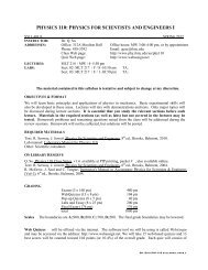
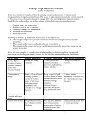
9. ANALYSIS SOFTWARE
Several commercial software packages are available on the the Macintoshes for mathematical,
graphical, and data analysis. These are additional tools available for solving physics problems. Most of
these packages come with extensive documentation, which the user should refer to regularly. This chapter
is merely intended to give a brief introduction to some of them.
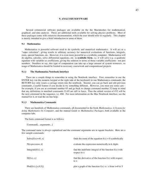
9.1 Mathematica
Mathematica is powerful software used to do symbolic and numerical mathematics. It will act as a
"super calculator", giving results to arbitrary accuracy for numerical evaluations of functions, integrals,
roots, special functions, etc. However, it is even more powerful as a symbolic computer. Mathematica will
do algebra, calculus, solve differential equations, etc. in symbolic form, i.e. it will solve e.g. a quadratic
equation with variables as coefficients, giving the solution in terms of those variable coefficients - not just
numbers. Needless to say, this type of computation can take up a large amount of system resources, so
usage of Mathematica should be limited to necessary coursework and computational projects.
9.1.1 The Mathematica Notebook Interface
There are a couple things to remember in using the Notebook interface. First, remember to use the
ENTER key (on the numeric keypad at the right side of the keyboard) to run Mathematica commands; the
RETURN key only issues a carriage return into the notebook. Second, you can go back and edit previous
commands, a useful feature if you decide to try something different. However, you must use some care -
for example, if you are at command number 65 and go back to change command number 32 keep in mind
that any definitions in unedited commands 33-65 are still in force. Thus the edited version of #32 will be
the next command in the sequence, i.e. #66. For more information on the Mac Notebook interface, see the
manual for it, or read the on-line help.
9.1.3 Mathematica Commands
There are hundreds of Mathematica commands, all documented in the book Mathematica: A System for
doing Mathematics by Computer, and the manual Guide to Mathematica Packages, both available in the
computer labs.
The basic command format is as follows:
Command[... arguments...]
The command name is always capitalized and the command arguments are in square brackets. Here are a
few sample commands:
Solve[f(x)==0, x]
N[expression, k]
Integrate[f(x), x]
D[f(x), x]
finds the roots of the equation f(x) = 0 symbolically
evaluate the expression numerically to k digits
find the indefinite integral of the function f(x) with
respect to x
find the derivative of the function f(x) with respect
to x
Plot[f(x),{x,0,5}] plot a graph of the function f(x) vs. x from x=0 to 5

44
Simple replacements can often be typed in using quasi-algebraic notation, such as the following
replacement commands defining the variable y:
y = x^2 + 23.4x^3 + 12.78 Pi
y = Sin[3 x]/ArcTan[x] + Exp[-b x^3]
When you type in a command, Mathematica labels the command sequentially, then gives the result as
output with the same label. Here’s an example:
Note that the symbol “%” means “the previous output”, while “Out[8]” refers specifically to output
number 8. Finally, the notation “expression /. x–>a” means to evaluate the expression at x = a.
These samples should get you started with simple commands, but you will rapidly need to consult the
manuals for more information as you learn the power and utility of the Mathematica program.

46
9.2 KaleidaGraph
KaleidaGraph is one of many similar graphics and calculation programs available for the Macintosh.
With it you can plot two-dimensional data in various formats, producing publication-quality results. It also
has many built-in functions for performing simple calculations with your data. Since the full KaleidaGraph
manual is available, we cover only the basics here: importing data and making simple plots.
9.2.1 Getting Data into KaleidaGraph
Start KaleidaGraph from the Apple menu or by double-clicking on the KaleidaGraph program or one
of its files. For small data sets you can simply type the numbers into the blank file that opens by default
when you start KaleidaGraph, i.e. position the cursor in a cell and start typing. You can use the mouse or
the arrow keys to move between cells. The TAB key moves right one cell and selects its contents - a handy
way to overwrite the data in that cell. The program is column-oriented, and you should type data in
columnar form. To give each data column a name, double-click on the top cell of the column to open the
menu showing properties of that column. In this menu you can change the title of the column, the data
format, and the column width. The title of the column is used as the axis label when you plot that column.
Set up the columns as you wish and then type in the data. When finished you are ready to plot, using the
Gallery menu, as described below. Figure 1 shows a sample data window from KaleidaGraph.
Figure 1. KaleidaGraph Data Window
When you produce data with another program (e.g. with FORTRAN), the output file is usually too
large to conveniently type in by hand. In this case, you can import the data directly into KaleidaGraph
containing columns of numbers. Here is the procedure:
1. Create the data file as a text (ASCII) file with columns of data, separated by at least one space.
For example, in FORTRAN you might use the following commands:
WRITE(10,’(F6.3,3x,F7.2)’) POSITION,TIME
2. If the file is not already on the Macintosh, transfer it using a program which can use ftp.

47
3. When you have the file on the MAC, start KaleidaGraph and choose “Open” from the File menu.
A window will pop up asking you to tell KaleidaGraph more about the text file it is to open. You
need to tell what delimiter you used, e.g. with the above FORTRAN statement, the data will
delimited by 3 spaces, so choose “Space” and “≥3” from the menu. It also allows you to skip
lines if there is data you don’t want in the KaleidaGraph file. When you click on “OK” the file
should open as a KaleidaGraph data window.
Data files might also be produced in lab experiments and stored on a DOS diskette. If this is the case, ask
your Professor how to get the data onto the Macintosh.
9.2.2. Plotting Data
With your data window open, simply choose the plot type from the Gallery menu; e.g. for the sample
data above (Figure 1), choose “linear” and “scatter” to plot individual data points, unconnected. A window
will pop up asking you what columns of data to use a x and y axes; choose time on the x-axis and position
on the y-axis. The plot will look like something like this:
Position
6
Sample KG Data
5
4
3
2
1
0
-0.2 0 0.2 0.4 0.6 0.8 1 1.2
Time
You can delete an object by clicking once on it and pressing the delete key on the keyboard (or
choosing “cut” from the edit menu). You can edit the plot by double-clicking on the object you want to
change. For example:
To change axis labels:
To change axis ticks:
To change the plot title:
To change data point symbols:
click on the axis label text; an edit window opens allowing you to
make changes as needed.
click on the axis itself; an edit window will open allowing you
make changes in tick locations, tick mark numbers, grid, etc.
click on the title and use the edit window.
click on the symbol above the graph (in the legend). A window
will open allowing several different symbols types and other
format options.

The graphical tools menu to the left of the plot allows further formatting, e.g. resizing the whole plot,
adding text or drawing, “windowing” in on a smaller region of the plot, etc. Try the tools to see what they
do, or consult the manual for further details.
48

49
9.2.3. Curve Fitting
KaleidaGraph allows various styles of curve fitting, including linear, polynomial, logarithmic, and
exponential. To fit the data in your plot, choose the type of fit you want from the Curve Fit menu. For
example, let’s fit the above data with a parabola; i.e. choose “polynomial” fit. A window opens up asking
which curve to fit (if you have multiple curves), then which degree of polynomial: choose 2nd degree for a
parabola. The result is (also including some cleaning up of axes):
6
sample KG data.txt
5
Position (cm)
4
3
2
1
Y = M0 + M1*x + ... M8*x 8 + M9*x 9
M0
0.25105499017
M1
2.0792304377
M2
2.8269760865
R
0.98539870081
0
0
0.2 0.4 0.6 0.8 1
Time (sec)
The box to the right shows the equation of the best-fit line and some curve fit statistics. If it doesn’t appear
when you do the fit, choose “Display Equation” from the Plot menu.
9.2.4. Multiple Curves
Plotting multiple curves is easy with KaleidaGraph. If your data file has three columns, for example,
and you want to plot columns 1 and 2 versus column 0, just choose c1 and c2 as the y-axis in the pop-up
window that appears when you choose your plot type.
If you want to plot data from different files on the same plot, open all the files simultaneously. Choose
the plot type as usual from the Gallery menu. The axis selection window then pops up and notice that the
box containing the file name for the top data file looks “3-Dimensional”, as if it has some thickness. This
is KaleidaGraph’s way of telling you that there is a pop-up menu under the box: click on it and hold the
mouse button down and you will see the names of all the open files. Select each one in turn and choose
which columns to put on the x and y axes. When you’re finished click “OK” and the plot will be made.
9.2.5. Formulas
To do computations with your data, use the formula window. If you can’t see it, choose “Formula
Entry” from the Windows menu. Type the formula you want to use in the window, e.g.:
c2 = c0^2 + exp(c1)
and click “OK”. Column 2 will be computed and added (or modified if it already exists) to the data
window. Check out the “Help” under the Apple menu to get a list of which functions KaleidaGraph knows.