Time-Dependent Electron Localization Function - Fachbereich ...
Time-Dependent Electron Localization Function - Fachbereich ...
Time-Dependent Electron Localization Function - Fachbereich ...

Create successful ePaper yourself
Turn your PDF publications into a flip-book with our unique Google optimized e-Paper software.
<strong>Time</strong>-<strong>Dependent</strong><br />
<strong>Electron</strong> <strong>Localization</strong> <strong>Function</strong><br />
Diplomarbeit by<br />
Tobias Burnus<br />
Adviser:<br />
Prof. Dr. E. K. U. Groß<br />
<strong>Fachbereich</strong> Physik<br />
Freie Universität Berlin<br />
2004
<strong>Time</strong>-<strong>Dependent</strong><br />
<strong>Electron</strong> <strong>Localization</strong> <strong>Function</strong><br />
Tobias Burnus<br />
The electron localization function ELF, which is crafted to reveal chemical bonds and<br />
their properties, has been generalized to the time-dependent regime. This allows the<br />
time-resolved visualization of the formation, modulation and breaking of bonds and<br />
gives thus insight into the dynamics of excited electrons. This has been illustrated<br />
by the π–π ∗ transition of ethyne induced by a laser field, and by the destruction of<br />
bonds and the formation of lone-pairs in a scattering process of a proton with ethene.<br />
In the second part, an optimal control algorithm is used to determine an optimized<br />
laser pulse of a HOMO–LUMO transition of the diatomic molecule lithium fluoride.<br />
Diplomarbeit · Adviser: Prof. Dr. E. K. U. Groß<br />
<strong>Fachbereich</strong> Physik, Freie Universität Berlin<br />
2004
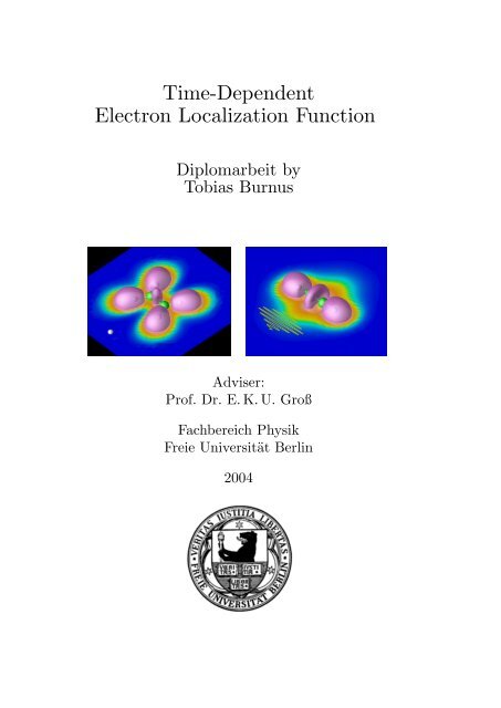
Title page: ELF images showing a proton on collision course with the left carbon of<br />
ethene (left) and ethyne (right) in a laser field polarized along the molecular axis.<br />
Published 26 January 2004<br />
Copyright © Tobias Burnus 2004.<br />
Everyone may use this work according to the terms and conditions of the Lizenz für die freie<br />
Nutzung unveränderter Inhalte (Licence for Free Usage of Invariable Content).<br />
The licence text can be obtained at http://www.uvm.nrw.de/opencontent or by writing to Geschäftsstelle<br />
des Kompetenznetzwerkes Universitätsverbund MultiMedia NRW, Universitätsstraße<br />
11, D-58097 Hagen, Germany.<br />
The use of registered names, trademarks etc. in this publication does not imply that such names<br />
are exempt from the relevant protective laws and regulations and therefore free for general use.<br />
Typeset using ConTEXt in Latin Modern and Computer Modern 12pt.<br />
images and movies have been created using OpenDX.<br />
The ELF and density
Dedication:<br />
For my parents<br />
i
We haven’t got the money, so we’ve got to think!<br />
— Ernest Rutherford, 1871–1937<br />
Preface<br />
A physics professor, teaching quantum mechanics, once said that one is not allowed<br />
to ask where the electrons are during the transition between two states. But<br />
nevertheless: How does a chemical bond such as a triple bond break? One knows<br />
from chemisty or molecular physics courses that there are bonding and anti-bonding<br />
states. But what happens exactly at which time. We know that the breaking of<br />
bonds happens on a time-scale of hundreds of attoseconds, which is the time-scale<br />
of the electrons. With the advance of attosecond spectroscopy, one might even be<br />
able two answer some of these questions experimentally.<br />
For tackling this problem, we describe the system using the density-functional theory<br />
which enables us to calculate molecules with many electrons and propagate such a<br />
system in time. We therefore give a short introduction into this theory in chapter 1,<br />
which is necessarily short and incomplete.<br />
Before we can ask how a chemical bond breaks, we need to know what actually<br />
defines a bond. This is not as simple as it seems, in the real world the atom<br />
does not know about orbitals which have been used to visualize and to understand<br />
the concept of a bond. The orbitals that stem from calculations, however, can be<br />
lineary combined or may be delocalized over several atoms. Using the density does<br />
not help much, either: The only maxima of the density are located at the nuclei<br />
and while there is density between bond atoms, it is hard to classify or even only to<br />
visualize the chemical bonds. The solution is to make use of the localizability of the<br />
electrons instead of utilizing the density directly. This does the the so-called electron<br />
localization function (ELF) which we cover in chapter 2. Up to now, the ELF had<br />
only been used for static systems or for those which can be described adiabatically.<br />
We have devised a version which can be utilized for time-dependent systems. This<br />
TDELF has then be used to scrutinize the effects of a strong laser (electric field)<br />
on ethyne and for scattering of fast protons by ethene. We were able to see how a<br />
transition from the π bonding to the π ∗ anti-bonding state was building up, bonds<br />
were breaking and re-forming, and lone-pairs emerging.<br />
Preparing a certain state, such as the π ∗ anti-bonding state, can be tricky if the<br />
exact transition energy is unknown or, in other cases, intermediate states exists.<br />
One possibility to create a tailored laser is provided by the various optimal control<br />
theories. We look at a functional based on optimal control theory in chapter 3.<br />
Since doing optimal control for a larger molecule requires a lot of book-keeping and<br />
computational resources, we started with a simpler example: The HOMO–LUMO<br />
iii
Preface<br />
transition of a cylinder-symmetric diatomic molecule. Using a such tailored laser,<br />
we achieved a population transfer of over eighty per cent from HOMO to LUMO in<br />
lithium fluoride.<br />
The final part of this thesis, chapter 4, contains conclusions and aspects which need<br />
further investigation.<br />
Throughout the thesis, two kind of units are used: the SI units and the atomic<br />
units (see appendix D for the conversion factor). Using the former, the numbers<br />
can easily be compared with experimental results. On the other hand, atomic units<br />
drop a lot of constants and the numerical results of atomic calculations can usually<br />
be written without exponentials. This makes atomic units ideal for both numerics<br />
and lengthy calculations. I hope that I found the right balance between these two<br />
common unit systems.<br />
Acknowledgement<br />
While it has become a custom to write an acknowledgment and it is often only a<br />
mere item on the list of the things which are part of a thesis, for me it has not<br />
lost its original meaning since I know that I would not have reached this point and<br />
finished the thesis without the help and support of various people. Regarding this<br />
diploma thesis I would like to express my special thanks to the following people.<br />
I feel deeply indebted to my adviser Professor Eberhard ‘Hardy’ K. U. Groß. I am<br />
grateful for his encouragement and support, the discussion we had and the impulses<br />
he gave me. While he was not always reachable, especially in the second half of<br />
the year when he was a guest at the University of Cambridge, he managed to be<br />
always available when needed. In addition, this proved to be an efficient way to<br />
stimulate the productive intra-group communication which otherwise might be not<br />
as intensive. Without him I would not have attended a summer school in Sweden,<br />
where I not only learnt a lot about DFT and could present my results but met new<br />
friends. Especially enjoyable were his group dinner meetings, where he sometimes<br />
even played the piano.<br />
I have benefitted from Miguel Marques who introduced me to octopus and helped<br />
me with all problems I had with it. His Fortran style as used in octopus influenced<br />
mine to the better. I also gained a lot from his experience especially in calculating<br />
larger systems and he helped me to tackle some analytical problems.<br />
Jan Werschnik is the expert of our group in optimal control and was therefore of<br />
tremendous help during the second part of the thesis, though as an office mate he<br />
he had to answer tons of little and not so little questions throughout the the whole<br />
year. I am especially grateful for his and Stephan Kurth’s help as I got stuck with<br />
the bondary conditions of the discretized matrix, where they kindly spend much of<br />
iv
Preface<br />
their spare time to crack this problem. Especially during this phase we had vivid<br />
and constructive discussions.<br />
I would like to thank Nicole Helbig, who always lend an sympathetic ear to me.<br />
She also helped me with some mathematical problems and was the driving force<br />
behind our group ice skatings. Furthermore, she, Stephan and Jan volenteered to<br />
give introductionary lectures about DFT just for us two Diplomanden.<br />
Thanks also to Heiko Appel who is a real treasure trove regarding articles, furthermore<br />
he helped me finding and choosing the right numerical methods. I would like<br />
to thank Angelica Zacarias who found a cylindrical diatomic molecule and did the<br />
Gaussian calculations. Finally, I want to express my thanks to the whole group who<br />
created a pleasant atmosphere; I really enjoyed that year.<br />
There are two further persons whom I would like to thank – my parents. They have<br />
supported and encouraged me, and where there when I needed them.<br />
v
Contents<br />
Contents<br />
Preface<br />
Acknowledgement<br />
Contents<br />
iii<br />
iv<br />
vii<br />
1 Density functional theory 1<br />
1.1 The Hohenberg--Kohn theorem 1<br />
1.2 The Kohn--Sham formalism 4<br />
1.3 <strong>Time</strong>-dependent DFT – the Runge--Groß theorem 7<br />
1.4 Pseudo potentials 8<br />
2 The time-dependent electron localization function 11<br />
2.1 Introduction 11<br />
2.2 The static electron localization function 13<br />
2.3 Derivation of the time-dependent ELF 14<br />
2.3.1 Spherical average and Taylor expansion of P σ (r, r + s, t) 15<br />
2.3.2 Derivation of D σ in the single-particle picture 17<br />
2.3.3 Calculation of C σ 19<br />
2.3.4 Comparison with the static ELF 20<br />
2.4 Application of the TDELF 21<br />
2.4.1 Excitation of molecules 21<br />
2.4.2 Proton scattering 23<br />
2.5 Conclusions 26<br />
3 Optimal control 29<br />
3.1 Introduction 29<br />
3.2 Algorithm 29<br />
3.2.1 Iteration algorithm 32<br />
3.3 Optimizing the HOMO–LUMO transition of LiF 33<br />
3.3.1 Calculation of Hψ i = ε i ψ i 33<br />
3.3.2 Discretization 36<br />
3.3.3 The five-point discretization 39<br />
3.3.4 Solving the eigenvalue problem 41<br />
3.3.5 <strong>Time</strong> propagation 41<br />
3.3.6 Absorbing boundaries 43<br />
3.4 Application of the optimal control algorithm 43<br />
3.5 Conclusions 51<br />
vii
Contents<br />
4 Conclusion 53<br />
A TDELF auxiliary calculations 55<br />
A.1 Simplification of C σ 55<br />
A.2 Deriving the time-dependent ELF for a simplified, two-particle case 57<br />
B Optimal control for many-particle systems 59<br />
B.1 Calculation of the overlap 〈 ˜Ψ|Ψ〉 59<br />
B.2 Calculation of the dipole moment 〈 ˜ψ| ˆX |ψ〉 60<br />
C Proof for the overlap of two Slater wave functions 65<br />
D Atomic, ‘convenient’ and SI Units 67<br />
D.1 Atomic Units 67<br />
D.2 ‘Convenient units’ 68<br />
D.3 Comparison and conversion 68<br />
D.4 Constants 68<br />
Abbreviations and Acronyms 71<br />
Used symbols 73<br />
References 75<br />
viii
1 Density functional theory<br />
A new scientific truth does not triumph by convincing its opponents<br />
and making them see the light, but rather because its<br />
opponents eventually die, and a new generation grows up that is<br />
familiar with it. — Max Planck, 1858–1947<br />
While traditional many-particle wave-function methods perform well for a wide<br />
range of systems, they come to their limits for non-symmetric or periodic systems<br />
with many (chemically active) electrons. That is because the numerical effort to<br />
calculate and store multi-particle wave functions grows exponentially with the number<br />
of electrons. Therefore, these methods can currently only be applied to systems<br />
with about ten chemically active electrons [1]. A solution to this exponential wall is<br />
density-functional theory (DFT). Several introductory texts on DFT can be found<br />
in the literature. Among them are Kohn’s Nobel lecture [1], the lecture notes by<br />
Perdew and Kurth [2], Burke’s ABC of DFT [3], or Taylor and Heinonen’s DFT<br />
chapter in [4]. For time-dependent DFT, the TD-Review by Groß et al. [5] provides<br />
a clear and in-depth introduction.<br />
This chapter provides a short overview of the theory but is not meant to give a<br />
complete and self-contained account about all aspects. The next section covers the<br />
Hohenberg--Kohn theorem, which proves that every observable can be written as<br />
a unique functional of the electron density. The Kohn--Sham theory, described in<br />
section 1.2, states that the density of an interacting system can be obtained using<br />
an effective single particle potential. This is then generalized to the time-dependent<br />
regime by the Runge--Groß theorem in section 1.3. The numerical effort can be<br />
further reduced by pseudopotentials described in section 1.4.<br />
1.1 The Hohenberg--Kohn theorem<br />
A quantum system of N particles can be completely described 1 by its Hamiltonian<br />
H = T + V + W . The Hamilton operator consists of the kinetic part<br />
T = − 2<br />
2m<br />
N∑<br />
∇ 2 i , (1.1)<br />
the interaction W , which – for the case of Coulomb interactions between electrons<br />
– has the form<br />
1 In this thesis we completely neglect effects which can only be described by quantum electrodynamics<br />
(QED).<br />
i=1<br />
1
Chapter 1: Density functional theory<br />
W = 1<br />
4πε 0<br />
N ∑<br />
i,j=1<br />
i
1.1 The Hohenberg--Kohn theorem<br />
But E − E ′ is a real number, so that means that the two potentials differ at most<br />
by a constant which is a contradiction to our hypothesis. We have thus shown that<br />
if V ≠ V ′ then Ψ 0 ≠ Ψ ′ 0 . We now look at the relation ship between the density<br />
and the wave function. Be n the ground-state density in the potential V with its<br />
corresponding ground-state wave function Ψ. Then the total energy is<br />
∫<br />
E = 〈Ψ|H|Ψ〉 = 〈Ψ|(T + W )|Ψ〉 + V (r)n(r) d 3 r. (1.8)<br />
Be V ′ another potential which differs from V by more than an additive constant<br />
and Ψ ′ be its associated wave function, which yields the same density n as Ψ does.<br />
The Rayleigh--Ritz minimal principle states that<br />
∫<br />
E < 〈Ψ ′ |H|Ψ ′ 〉 = 〈Ψ ′ |(T + W )|Ψ ′ 〉 + V (r)n(r) d 3 r<br />
= E ′ +<br />
∫ (V<br />
(r) − V ′ (r) ) n(r) d 3 r, (1.9)<br />
where we have used that n ′ ≡ n by assumption. Analogously we find for E ′ ,<br />
Adding Eq. (1.9) and Eq. (1.10), gives<br />
E ′ < E +<br />
∫ (V ′ (r) − V (r) ) n(r) d 3 r. (1.10)<br />
E + E ′ < E + E ′ +<br />
∫ (V<br />
(r) − V ′ (r) + V ′ (r) − V (r) ) n(r) d 3 r = E + E ′ . (1.11)<br />
This is a contradiction to the assumption that both Ψ and Ψ ′ have the same groundstate<br />
density. We have thus established that two different, non-degenerate ground<br />
states lead to different ground-state densities. We further know that different potentials<br />
lead to different wave functions. Therefore, we proved that knowing the<br />
ground-state density n(r) of a system is sufficient to construct the external potential<br />
(if n is V -representable).<br />
There is also an important variational principle associated with the Hohenberg--<br />
Kohn theorem. We know that the electronic ground-state energy can be obtained<br />
by making use of the Rayleigh--Ritz principle,<br />
E = min 〈 ˜Ψ|H| ˜Ψ〉, (1.12)<br />
˜Ψ∈{ ˜Ψ}<br />
where { ˜Ψ} is the set of all normalized, antisymmetric N-particle wave functions.<br />
Hohenberg and Kohn showed that the Rayleigh--Ritz principle can also be applied<br />
to the energy functional,<br />
3
Chapter 1: Density functional theory<br />
∫<br />
E[n] = 〈Ψ 0 [n]|(T + W + V )|Ψ 0 [n]〉 = F HK [n] +<br />
V (r)n(r) d 3 r, (1.13)<br />
where Ψ 0 is the ground-state wave function and<br />
F HK [n] = 〈Ψ 0 [n]|(T [n] + W [n])|Ψ 0 [n]〉. (1.14)<br />
The ground-state energy can be found by varying the density, i. e.<br />
( ∫<br />
)<br />
E = min<br />
ñ∈Ñ<br />
F HK [ñ] + ñ(r)V (r) d 3 r , (1.15)<br />
where Ñ is the set of all V -representable trial densities. In other words, the minimum<br />
of this functional can only be reached with the ground-state density corresponding<br />
to the potential V (r). In this case the value of the functional is the ground-state<br />
energy.<br />
Note that the functional F HK [n] is a universal functional. By this we mean that it<br />
is the same functional of the density n(r) for all N-particle systems, which have<br />
the same kind of interaction (e. g. Coulomb). Especially, it is independent of the<br />
external potential V . Therefore, we need to approximate it only once and can then<br />
apply it to all systems.<br />
1.2 The Kohn--Sham formalism<br />
While the Hohenberg--Kohn theorem establishes that we may use the density alone<br />
to find the ground-state energy of an N-electron problem, it does not provide us<br />
with any useful computational scheme. This is accomplished by the Kohn--Sham<br />
(KS) formalism [7]. The idea is to use an auxiliary, non-interacting system and to<br />
find an external potential V KS such that this non-interacting system has the same<br />
electron density as the real, interacting system. This density can then be used in the<br />
energy functional (Eq. (1.13)). The ground-state of the Kohn--Sham system is given<br />
by a Slater determinant of the N lowest, single-particle states of the Hamiltonian<br />
which contains V KS . While this provides us with a route for calculations, there<br />
is a drawback. The potential V KS depends on the electron density (see below).<br />
Therefore, the potential has to be found iteratively in a self-consistent way.<br />
Let us start with the non-interacting N-particle system described by the external<br />
potential V KS . The Hamiltonian of the system is given by<br />
The ground-state density of this system has the form<br />
H = T + V KS . (1.16)<br />
4
1.2 The Kohn--Sham formalism<br />
n(r) =<br />
N∑<br />
|φ i (r)| 2 , (1.17)<br />
i=1<br />
where the N single-particle orbitals φ i in Eq. (1.17) satisfy the Schrödinger equation<br />
)<br />
(− 2<br />
2m ∇2 + v KS (r) φ i (r) = ε i φ i (r), (1.18)<br />
and have the N lowest eigenenergies ε i . The total energy of the ground-state of the<br />
non-interacting system is therefore<br />
E KS =<br />
N∑<br />
ε i . (1.19)<br />
Note that the value of this energy does not correspond to the ground-state energy<br />
of the interacting system. According to the Hohenberg--Kohn theorem, it exists a<br />
unique energy functional<br />
∫<br />
E KS [n] = T KS [n] + V KS (r)n(r) d 3 r. (1.20)<br />
We note that T KS [n] is the kinetic energy functional of the non-interacting system<br />
and it is therefore different from the functional T [n] in Eq. (1.14). In order to solve<br />
the interacting system, we need to find a form of V KS , so that the ground-state<br />
densities of the non-interacting and the interacting system are the same. Since we<br />
are really interested in the interacting system, we rewrite Eq. (1.13) as<br />
∫<br />
E[n] = T [n] + W [n] + n(r)V (r) d 3 r (1.21)<br />
= T KS [n] + 1 e 2<br />
4πε 0 2<br />
∫ ∫ n(r)n(r ′ )<br />
|r − r ′ |<br />
i=1<br />
∫<br />
d 3 r d 3 r ′ +<br />
n(r)V (r) d 3 r + E xc [n].<br />
Here, the second term is the direct, or Hartree, term and the last term is the so-called<br />
exchange-correlation (xc) energy functional, defined as<br />
E xc [n] = F HK [n] − 1 e 2 ∫ ∫ n(r)n(r ′ )<br />
4πε 0 2 |r − r ′ d 3 r d 3 r ′ − T KS [n]. (1.22)<br />
|<br />
With this formalism at hand, one only needs to develop reasonable approximations<br />
for E xc , which contain the electron–electron interaction beyond the Hartree term<br />
5
Chapter 1: Density functional theory<br />
and the difference in the kinetic energy functionals T [n] − T KS [n]. Since the groundstate<br />
density n minimizes the functional E[n], we obtain by varying Eq. (1.21) in<br />
terms of the density, 3<br />
δE[n]<br />
δn(r) = δT KS[n]<br />
δn(r) + 1 ∫ n(r<br />
e 2 ′ )<br />
4πε 0 |r − r ′ | d3 r ′ + V (r) + v xc [n](r) = 0, (1.23)<br />
where we defined the exchange-correlation potential as<br />
v xc [n](r) := δE xc[n]<br />
δn(r) . (1.24)<br />
Analogously, for the auxiliary system we obtain from Eq. (1.20)<br />
δT KS [n]<br />
δn(r) + V KS(r) = 0. (1.25)<br />
Subtracting Eq. (1.23) from Eq. (1.25), we see that the effective, or Kohn--Sham,<br />
potential has to satisfy<br />
V KS (r) = V (r) + 1<br />
4πε 0<br />
e 2 ∫ n(r ′ )<br />
|r − r ′ | d3 r ′ + v xc (r). (1.26)<br />
Now we could start implementing the self-consistent Kohn--Sham scheme. Note<br />
that this formalism is in principle exact, supposing that we find the exact exchangecorrelation<br />
potential v xc . Solving a Kohn--Sham system with single-particle orbitals<br />
is feasible even for systems with a few hundred electrons (cf. [1, 4]). Formally,<br />
the Kohn--Sham equations look similar to the self-consistent Hartree equations, the<br />
only difference is the exchange-correlation potential. Neither φ i nor ε i have any<br />
known, directly observable meaning, except that the φ i yield (in principle) the true<br />
ground-state density and that the magnitude of the highest occupied ε i , relative to<br />
the vacuum, equals the ionization energy [8].<br />
One famous approximation for the exchange-correlation energy is the local density<br />
approximation (LDA) by Kohn and Sham [7].<br />
∫<br />
Exc LDA [n] := n(r)ε uni (n(r)) d 3 r, (1.27)<br />
where ε uni denotes the exchange-correlation energy per particle of a uniform electron<br />
gas with the density n. ε uni (n) can be obtained using quantum Monte Carlo<br />
calculations [9].<br />
3 Note though that ‘the KS scheme does not follow from the variational principle. [. . . ] The KS<br />
scheme follows from the basic 1-1 mapping (applied to non-interacting particles) and the assumption<br />
of non-interacting V -representability.’ [5]<br />
6
1.3 <strong>Time</strong>-dependent DFT – the Runge--Groß theorem<br />
1.3 <strong>Time</strong>-dependent DFT – the Runge--Groß theorem<br />
The time-dependent density-functional theory (TDDFT) extends the stationary<br />
DFT in a way that not only makes time-dependent phenomena available to computation,<br />
but it also provides a natural way to calculate excitations of a system.<br />
For static systems, we have seen how the Hohenberg--Kohn theorem establishes a<br />
one-to-one correspondence between the external potential and the density. We now<br />
look at systems, where the external potential V depends explicitly on time. We<br />
start with the time-dependent Schrödinger equation<br />
For the theorem, a fixed initial state<br />
i∂ t Ψ(t) = H(t)Ψ(t). (1.28)<br />
Ψ(t 0 ) = Ψ 0 (1.29)<br />
is required, which is not required to be an eigenstate of the initial Hamiltonian.<br />
While the kinetic part T and the electron–electron interaction W remain unchanged<br />
compared to static DFT, the potential V becomes time-dependent<br />
V (t) =<br />
N∑<br />
v(r i , t). (1.30)<br />
i=1<br />
The theorem by Runge and Gross [10] now states: If the potentials V and V ′ (both<br />
Taylor expandable around t 0 ) differ by more than a purely time-dependent but<br />
spatially uniform function, i. e.<br />
V (r, t) ≠ V ′ (r, t) + c(t), (1.31)<br />
then the densities n(r, t) and n ′ (r, t), evolving from the common initial state Ψ 0<br />
under the influence of the two potentials, are different. For the proof, both potentials<br />
are Taylor expanded in time. Then a k ∈ N exists so that the difference beween<br />
the k-th Taylor coefficients is not constant, i. e. the difference is r dependent. The<br />
proof [5, 10] shows next that under these circumstances the current densities become<br />
different and then that the densities are different.<br />
For any given time-dependent density n (and initial state Ψ 0 ) the external potential<br />
can be determined uniquely up to an additive purely time-dependent function; and<br />
this potential uniquely determines the wave function, up to a purely time-dependent<br />
phase. This phase cancels if we calculate the expectation value of any quantum<br />
mechanical operator O[n](t) = 〈Ψ[n](t)|O(t)|Ψ[n](t)〉. Thus any observable is a<br />
unique functional of the time-dependent density and of the initial state Ψ 0 .<br />
7
Chapter 1: Density functional theory<br />
Once the Runge--Groß theorem is established, one can continue and derive the<br />
Kohn--Sham equations [5, 10]. The density of the interacting system can be obtained<br />
from<br />
n(r, t) =<br />
N∑<br />
|φ i (r, t)| 2 (1.32)<br />
i=1<br />
with the orbitals φ i satisfying the time-dependent Kohn--Sham equation<br />
)<br />
i∂ t φ i (r, t) =<br />
(− 2<br />
2m ∇2 + v KS [n](r, t) φ i (r, t). (1.33)<br />
The Kohn--Sham, or single-particle, potential can be written as<br />
v KS [n](r, t) = V (r, t) +<br />
where V (r, t) is the time-dependent external field.<br />
∫ e2 n(r ′ , t)<br />
4πε 0 |r − r ′ | d3 r + v xc [n](r, t) (1.34)<br />
1.4 Pseudo potentials<br />
Chemical reactions and excitations with energies below X-ray wavelengths hardly<br />
affect closed inner shells. Therefore, the many-particle Schrödinger equation can be<br />
simplified to a great extent by dividing the electrons into two groups: valence and<br />
inner core electrons. Since the inner core electrons are strongly bound, the chemical<br />
properties are almost completely determined by the valence electrons. Formally,<br />
one can create an effective interaction of the valence electrons with the ionic core,<br />
which consists of the nuclei and the inner core electrons. This pseudopotential<br />
approximates the potential felt by the valence electrons. The main advantage of<br />
pseudopotentials is the reduced numerical effort. This is the case since one has to<br />
consider only the valence orbitals. In addition, the problems with the 1/r potential<br />
(Coulomb singularity for r → 0) is eliminated. Therefore, a wider grid is viable.<br />
The tutorial by Nogueira et al. [11] and Pickett’s article [12] are good primers on<br />
pseudopotentials. In the following, a brief summary of the important properties and<br />
downsides is given.<br />
Modern pseudopotentials (PP) are obtained by inverting the Schrödinger equation<br />
for a given reference electronic configuration and forcing the pseudo wave function<br />
to coincide with the all-electron valence wave function beyond a certain distance r l .<br />
The pseudo wave functions are also forced to have the same norm as the all-electron<br />
wave functions. This can be written as<br />
8
1.4 Pseudo potentials<br />
∫ rl<br />
0<br />
R PP<br />
l<br />
r 2 |R PP<br />
l (r)| dr =<br />
(r) = Rnl AE (r), if r > r l,<br />
∫ rl<br />
0<br />
r 2 |R AE<br />
nl (r)| dr, if r < r l, (1.35)<br />
where R l (r) is the radial part of the wave function with angular momentum l. AE<br />
denotes the all-electron wave function and the index n the valence level. Note that<br />
the distance r l , beyond which the all-electron and the pseudo wave function are<br />
equal, depends on the angular momentum l. Moreover, pseudo wave functions shall<br />
not have nodal surfaces and the pseudo energy eigenvalues ε PP<br />
l<br />
should match the<br />
all-electron valence eigenvalues ε AE<br />
nl<br />
. Potentials constructed in this way are called<br />
norm conserving, and are semi-local potentials that depend on the energies of the<br />
reference electronic levels ε AE<br />
l<br />
. Unfortunately, pseudopotentials may introduce new,<br />
non-physical states (so called ghost states) into the calculation, so care must be<br />
taken while generating the pseudopotential.<br />
The choice of the cut-off radii establishes only the region where the pseudo and the<br />
all-electron wave function coincide. They can thus be considered as a measure of<br />
the quality of the pseudopotential. Their smallest possible value is determined by<br />
the location of the outermost nodal surface of the all-electron wave functions. For<br />
cut-off radii close to this minimum, the pseudopotential is very realistic and strong;<br />
for large r l , the potential is smooth, almost independent of angular momentum, but<br />
not very realistic. Since the pseudopotentials have no nodal surface and are smooth,<br />
much fewer grid points are needed near the core and thus uniform grids are feasible.<br />
octopus [13], which has been used for the ELF calculations in this work (see<br />
section 2) and for obtaining a Kohn--Sham potential (optimal control, section 3),<br />
supports the Hartwigsen--Goedecker--Hutter (HGH) [14] and the Troullier--Martins<br />
(TM) [15] pseudopotentials. The HGH pseudopotentials are norm-conserving, dualspace<br />
Gaussian pseudopotentials. The coefficients for all elements between H and<br />
Rn can be found in [14]. Troullier and Martins defined the pseudo wave functions<br />
as<br />
{<br />
Rl PP R<br />
AE<br />
(r) := nl (r), if r > r l<br />
r l e p(r) , (1.36)<br />
, if r < r l<br />
where<br />
p(r) = c 0 + c 2 r 2 + c 4 r 4 + c 6 r 6 + c 8 r 8 + c 10 r 10 + c 12 r 12 . (1.37)<br />
The coefficients of p(r) are adjusted by imposing norm conservation, the continuity<br />
of the pseudo wave functions and their first derivative at r = r l . Furthermore, it is<br />
required that the screened pseudopotential has zero curvature at the origin.<br />
9
Chapter 1: Density functional theory<br />
10
2 The time-dependent<br />
electron localization function<br />
What I cannot create, I do not understand.<br />
— Richard Phillips Feynman, 1918–88<br />
The electron localization function (ELF) is used to classify and visualize chemical<br />
bonds. In the next section, an introduction into the description of chemical bonds<br />
and the usefulness of the ELF is given. Afterwards, we look at the definition of<br />
the static ELF, constructed by Becke and Edgecombe, in section 2.2. Next, in<br />
section 2.3 we derive a time-dependent generalization of the ELF. This TDELF is<br />
then used to visualize the π–π ∗ transition of ethyne in a strong laser pulse and the<br />
breaking and formation of bonds in a scattering process of a proton with ethene in<br />
section 2.4. Finally, the conclusions of this chapter can be found in section 2.5.<br />
2.1 Introduction<br />
Already in the chemistry classes of secondary schools chemical bonds are introduced.<br />
The concept of a bond presented there and also in the undergraduate courses is<br />
reasonable clear and comprehensive; they are typically defined [16] as:<br />
chemical bond. A strong force of attraction holding atoms together in a<br />
molecule or crystal. Typically chemical bonds have energies of about 1000 kJ·<br />
mol −1 and are distinguished from the much weaker forces between molecules<br />
([. . . ] van der Waals’ forces). There are various types. Ionic (or electrovalent)<br />
bonds can be formed by transfer of electrons. [. . . ] Covalent bonds are formed<br />
by sharing of valence electrons rather than by transfer. [. . . ] A particular type<br />
of covalent bond is one in which one of the atoms supplies both the electrons.<br />
These are known as coordinate (semipolar or dative) bonds [. . . ]. Covalent<br />
or coordinate bonds in which one pair of electrons is shared are electron-pair<br />
bonds and are known as single bonds. Atoms can also share two pairs of<br />
electrons to form double bonds or three pairs in triple bonds.<br />
The idea of a bond is thus the sharing of electrons of neighbouring atoms whose<br />
orbitals overlap. This is the classical Lewis picture of bonding [17]. Transforming<br />
this concept into a mathematically rigorous scheme for classifying chemical bonds<br />
turns out to be astonishingly difficult. While using orbitals works well for small<br />
systems, this becomes cumbersome for larger systems. Especially, since the oneelectron<br />
wave functions that stem from Hartree--Fock or density-functional theory<br />
calculations are generally quite delocalized over several atoms and do not represent<br />
11
Chapter 2: The time-dependent electron localization function<br />
a unique bond. In addition, Hartree--Fock orbitals are ambiguous with regard to<br />
unitary transformations among the occupied orbitals. The total energy does not<br />
change under such transformations. Kohn--Sham orbitals are ambiguous only if<br />
they are degenerate.<br />
In the density, which contains all observable information, the bonds and their nature<br />
are only barely visible; features like lone pairs are especially hidden. Moreover, the<br />
density plots differ from the classical Lewis picture, where the charge is accumulated<br />
in the mid of covalent-bond atoms. Density plots show no local maxima in the bond<br />
region between the nuclei. There are basically two approaches which are nowadays<br />
used to classify chemical bonds: The Laplacian of the density −∇ 2 n introduced by<br />
Bader in 1984 [18] and the electron localization function constructed by Becke and<br />
Edgecombe in 1990 [19]. Both methods show essential similarities in their structure.<br />
(For a comparison of the two, see Bader’s article [20].) The Laplacian of the electron<br />
density seems to be superior for partial pairing of electrons as in acid–base reactions,<br />
while the ELF is more useful for comparing bonds [20]. In the following we focus<br />
on the ELF which is widely used in chemistry [21].<br />
The ELF is a functional of the density and the orbitals, designed to visualize the<br />
bonding properties. It was originally used for electronic shells of atoms, where it<br />
shows all shells (while other methods like the Laplacian of the density −∇ 2 n fail<br />
to show more than five shells), and for covalent bonds [19]. Subsequently, it has<br />
been used to analyze lone pairs, hydrogen bonds [22], surfaces [23], ionic and metallic<br />
bonds [23], and solids [23–25]. In addition, the ELF has the nice property of<br />
being rather insensitive to the method used to calculate the wave functions of the<br />
system: Hartree--Fock, density-functional theory or even extended Hückel methods<br />
yield quantitatively similar results [23]. The ELF can also be constructed from<br />
experimentally measured electron densities using X-ray data [25], utilizing an approximate<br />
functional for the dependence of the kinetic energy density on the electron<br />
density.<br />
The (static) ELF as constructed by Becke and Edgecombe can only be used to study<br />
systems in their ground state. Extending it to the time-dependent regime opens the<br />
possibility to study the creation, breaking or changing of bonds [26]. Examples of<br />
these include scattering processes (see section 2.4.2) and the excitation by a laser<br />
(see section 2.4.1), where a wealth of non-linear phenomena such as multi-photon<br />
ionization or high-harmonic generation can occur. Such phenomena happen on a<br />
time-scale of few femtoseconds, which can be examined using ulta-short laser pulses<br />
[27–29].<br />
12
2.2 The static electron localization function<br />
2.2 The static electron localization function<br />
The (static) electron localization function, developed by Becke and Edgecombe [19],<br />
is a descriptor of chemical bonding based on the Pauli exclusion principle. The<br />
correlation between the ELF and chemical bonding is a topological and not an<br />
energetic one, i. e. the ELF represent the organization of chemical bonding in real<br />
space [21, 30]. The local maxima of the function define localization attractors, which<br />
can be attributed to bonds, lone pairs, atomic shells and other elements of chemical<br />
bonding [21]. The resulting isosurfaces of the ELF densities tend to conform to the<br />
classical Lewis picture of bonding.<br />
In Slater determinant formulation 4 , the probability of finding two particles with the<br />
same spin, located at r and r ′ , is<br />
D σ (r, r ′ ) = n σ (r)n σ (r ′ ) − ∣ ∣n σ (r, r ′ ) ∣ ∣ 2 , (2.1)<br />
where D σ (r, r ′ ) is the same-spin pair probability and n σ (r) is the σ-spin singleparticle<br />
density matrix,<br />
∑N σ<br />
n σ (r, r ′ ) = φ ∗ iσ(r)φ iσ (r ′ ). (2.2)<br />
i=1<br />
The probability to find an electron at r ′ , knowing with certainty that a like-spin<br />
reference electron is at r, is given by the conditional pair probability<br />
P σ (r, r ′ ) = n σ (r ′ ) − |n σ(r, r ′ )| 2<br />
, (2.3)<br />
n σ (r)<br />
which is invariant with respect to unitary transformations. Since only the local,<br />
short-range behaviour is of interest, the spherically averaged conditional pair probability<br />
p σ is Taylor expanded. We obtain<br />
(<br />
p σ (r, s) = 1 Nσ<br />
)<br />
∑<br />
|∇φ iσ | 2 − 1 |∇n σ | 2<br />
s 2 + O(s 3 ), (2.4)<br />
3<br />
4 n σ<br />
i=1<br />
where (r, s) denotes the spherical average on a shell of the radius s around the<br />
reference point r. In the Taylor expansion, the first s-independent term vanishes<br />
due to the Pauli principle, also the term linear in s vanishes (see section 2.3.1 or<br />
[31]). We define τ σ as the positive-definite kinetic energy density<br />
4 This means, the wave function is written as determinant of single-particle wave functions; this<br />
single-particle picture encompasses the Kohn--Sham and Hartree--Fock formalism.<br />
13
Chapter 2: The time-dependent electron localization function<br />
∑N σ<br />
τ σ = |∇φ iσ | 2 . (2.5)<br />
i=1<br />
and can now write the s 2 coefficient of Eq. (2.4) as<br />
C σ (r) := τ σ − 1 |∇n σ | 2<br />
. (2.6)<br />
4 n σ<br />
This function, evaluated at the reference point, contains information about the electron<br />
localization. The smaller the probability of finding a second like-spin electron<br />
near r, the higher localized is this reference electron. C σ is not bounded from above,<br />
and approaches zero for strongly localized systems.<br />
Becke and Edgecombe defined [19] the electron localization function as<br />
where C uni<br />
σ<br />
ELF =<br />
1<br />
1 + ( C σ (r) ) 2 /<br />
(<br />
C<br />
uni<br />
σ (r) ) 2 , (2.7)<br />
denotes the kinetic energy density of the uniform electron gas<br />
C uni<br />
σ (r) = 3 5 (6π2 ) 2/3 n 5/3<br />
σ (r) =: τσ uni (r). (2.8)<br />
Contrary to C σ , the ELF is restricted to values between zero and one. A value of<br />
1 stands for perfect localization and 1/2 for the complete delocalization (uniform<br />
electron gas).<br />
Since this derivation [19] of the ELF assumes that the φ iσ are real, Eq. (2.6) is only<br />
valid for the static case, where the φ iσ can be chosen to be real. In the next section,<br />
we derive a C σ and thus an ELF without this restriction.<br />
2.3 Derivation of the time-dependent ELF<br />
In this section, we generalize the static electron localization function to complex wave<br />
functions, which is required for a time-dependent treatment. We follow essentially<br />
the steps by Becke and Edgecombe [19], but do not assume Hartree--Fock, i. e. Slater<br />
determinant, wave functions from the start (cf. [32]).<br />
The reduced single-particle density matrix is defined as<br />
∑<br />
∫ ∫<br />
n σ (r, r ′ , t) = N σ d 3 r 2 · · · d 3 r N Ψ ∗ (rσ, r 2 σ 2 , . . . , r N σ N , t)<br />
σ 2···σ N<br />
×Ψ(r ′ σ, r 2 σ 2 , . . . , r N σ N , t), (2.9)<br />
where Ψ is an N-electron wave function. For r = r ′ , it is known as spin density<br />
14
2.3 Derivation of the time-dependent ELF<br />
n σ (r, t) := n σ (r, r, t). (2.10)<br />
Eq. (2.10) gives the probability of finding a particle with spin σ at r and is normalized<br />
to the particle number N σ . For the ELF we need the spin-diagonal (σ 1 = σ 2 )<br />
of the reduced two-particle density matrix<br />
D σ1 σ 2<br />
(r 1 , r 2 , t) = N(N − 1) ∑ ∫ ∫<br />
d 3 r 3 · · · d 3 r N |Ψ(r 1 σ 1 , r 2 σ 2 , . . . , r N σ N , t)| 2 ,<br />
σ 3···σ N<br />
(2.11)<br />
which describes the probability of finding an electron with spin σ 1 at r 1 and another<br />
electron at r 2 with spin σ 2 . For σ 1 = σ 2 , it is known as the same-spin pair probability.<br />
Central for the electron localization function is the so-called conditional pair<br />
probability. It is defined analogously to the static case as<br />
P σ (r, r ′ , t) := D σσ(r, r ′ , t)<br />
n σ (r, t)<br />
(2.12)<br />
and gives the probability of finding an electron with spin σ at r ′ at time t knowing<br />
with certainty that another electron with the same spin is at r at that time.<br />
2.3.1 Spherical average and Taylor expansion of P σ (r, r + s, t)<br />
Since we are only interested in the probability of finding an electron in the vicinity<br />
of r, we substitute r ′ by r + s and do a spherical average of the Taylor expansion<br />
in s for small s, s := |s|.<br />
Expanding the wave function in terms of s (in the second argument) gives<br />
Ψ(rσ, (r + s)σ, . . . , r N σ N , t) = Ψ(rσ, (r + s)σ, . . . , r N σ N , t) ∣ s=0<br />
∣ 3∑ ∂Ψ ∣∣∣si<br />
+ s i + O(s 2 ). (2.13)<br />
∂s i =0<br />
The first term surely vanishes since two electrons with the same spin cannot be at<br />
the same location (Pauli exclusion principle). Thus we get<br />
|Ψ| 2 ∝<br />
3∑<br />
i,k=1<br />
i=1<br />
s i s k c ik + O(s 3 ), (2.14)<br />
where c ik contains the factors and the s-independent derivative of Ψ and Ψ ∗ . s can<br />
be written in spherical coordinates as s = (s 1 , s 2 , s 3 ) T = s (cos φ s sin θ s , sin φ s sin θ s , cos θ s ) T .<br />
Doing the spherical average of Eq. (2.14) leads to<br />
15
Chapter 2: The time-dependent electron localization function<br />
〈|Ψ| 2 〉 sph.av. ∝<br />
3∑<br />
∫<br />
c ii<br />
i=1<br />
s i s i dΩ +<br />
3∑<br />
∫<br />
c ik<br />
i,k=1<br />
i≠k<br />
s i s k dΩ + O(s 3 ). (2.15)<br />
Evaluating the integrals gives<br />
and<br />
〈s i s j 〉 sph.av. := 1<br />
4π<br />
∫<br />
s i s j dΩ = 0, i ≠ j (2.16)<br />
〈s 2 i 〉 sph.av. = 1 3 s2 , (2.17)<br />
and thus 〈|Ψ| 2 〉 sph.av. ˙∝s 2 . We define p σ as the spherical average of P σ<br />
and do a Taylor expansion<br />
p σ (r, s, t) := 〈P σ (r, r + s, t)〉 sph.av. . (2.18)<br />
p σ (r, s)<br />
1<br />
∑<br />
= N(N − 1)<br />
n σ (r, t)<br />
˙=<br />
1<br />
∑<br />
N(N − 1)<br />
n σ (r, t)<br />
σ 3 ,...,σ N<br />
∫<br />
σ 3 ,...,σ N<br />
∫<br />
∫<br />
d 3 r 3 · · ·<br />
∫<br />
d 3 r 3 · · ·<br />
d 3 r N 〈|Ψ| 2 〉 sph.av. (2.19)<br />
d 3 r N<br />
s 2<br />
3<br />
3∑<br />
( ∂<br />
i=1<br />
∂s i<br />
Ψ ∗ )s=0<br />
( ) ∂<br />
Ψ .<br />
∂s i s=0<br />
Since Ψ| s=0 = 0 and hence<br />
2<br />
3∑<br />
∂ si Ψ ∗ ∂ si Ψ∣ = ∇ 2<br />
s=0<br />
s|Ψ| 2∣ ∣<br />
∣s=0 = ∇ 2 r ′|Ψ(rσ, r′ σ, . . .)| 2∣ ∣<br />
∣r=r , (2.20)<br />
′<br />
i=1<br />
Eq. (2.19) can be simplified to<br />
p σ (r, s, t) = 1 3 s2 ( 1<br />
2<br />
∇ 2 r ′ D σ (r, r ′ , t)<br />
n σ (r, t)<br />
)∣<br />
∣∣∣r=r<br />
′<br />
+ O(s 3 ) ≡ 1 3 s2 C σ (r, t) + O(s 3 ). (2.21)<br />
The term in the bracket<br />
C σ = 1 2<br />
∇ 2 r ′ D σ (r, r ′ , t)<br />
n σ (r, t)<br />
∣<br />
r=r ′,<br />
(2.22)<br />
is a measure of the electron localization (cf. section 2.2). A small value of C σ (r)<br />
denotes a small probability of finding another electron near r. Thus there is a high<br />
electron localization at r which repels other like-spin electrons. In order to use C σ<br />
16
2.3 Derivation of the time-dependent ELF<br />
in density-functional calculations, we need to express D σ and n σ (r ′ , r, t) in terms<br />
of single-particle wave functions, which we do in the next sections.<br />
2.3.2 Derivation of D σ in the single-particle picture<br />
We now evaluate D σ and n σ using Slater determinant wave functions. In the following,<br />
π and µ denote permutations, π i and µ i the i-th component of a given<br />
permutation (i. e. π = (π 1 , . . . , π N )), and sgn π the sign of the permutation π.<br />
With these definitions, a determinantal wave function containing N = N σ orbitals,<br />
Φ iσ = Φ i , is given by<br />
∣ ∣∣∣∣∣<br />
Ψ det (r 1 , . . . , r N , t) = √ 1 det{φ i (r j , t)} = √ 1 φ 1 (r 1 , t) · · · φ 1 (r N , t)<br />
.<br />
... .<br />
N! N! φ N (r 1 , t) · · · φ N (r N , t)<br />
∣<br />
= √ 1 ∑<br />
sgn π φ 1 (r π1 , t) · · · φ N (r πN , t).<br />
N!<br />
π<br />
(2.23)<br />
By definition, the following identities are true: (sgn π) 2 = 1 and<br />
∫<br />
φ ∗ i (r, t)φ j (r, t) d 3 r = δ ij . (2.24)<br />
We now insert the Slater determinant wave function into the single-particle density<br />
matrix Eq. (2.9) and obtain<br />
n σ (r, r ′ , t)<br />
= N ∫ ∫<br />
∑<br />
d 3 r 2 · · · d 3 r N sgn π sgn µ φ ∗ π<br />
N!<br />
1<br />
(r 1 , t)φ µ1 (r 1 , t), · · · φ ∗ π N<br />
(r N , t)φ µN (r N , t)<br />
π,µ<br />
= N ∑<br />
(∫<br />
)<br />
sgn π sgn µ φ ∗ π<br />
N!<br />
1<br />
(r ′ , t)φ µ1 (r, t) d 3 r 2 φ ∗ π 2<br />
(r 2 , t)φ µ2 (r 2 , t) · · ·<br />
π,µ<br />
} {{ }<br />
δ π2 µ 2<br />
(∫<br />
)<br />
× d 3 r N φ ∗ π N<br />
(r N , t)φ µN (r N , t) . (2.25)<br />
} {{ }<br />
δ πN µ N<br />
We therefore know that all terms with π i ≠ µ i , i = 2, . . . , N vanish, and due<br />
to the definition of permutations, π 1 and µ 1 have to be identical. Thus π = µ,<br />
sgn π = sgn µ, and Eq. (2.25) simplifies to<br />
17
Chapter 2: The time-dependent electron localization function<br />
n σ (r, r ′ , t) = N ∑<br />
N∏<br />
φ ∗ π<br />
N! 1<br />
(r ′ , t)φ µ1 (r, t) δ πi π i<br />
π<br />
i=2<br />
} {{ }<br />
N! terms<br />
= N N N! (N − 1)! ∑<br />
φ ∗ l (r ′ , t)φ l (r, t) =<br />
l=1<br />
} {{ }<br />
N terms<br />
Following an analogous route for D σ , we obtain<br />
D σ (r, r ′ , t) =<br />
N(N − 1)<br />
N!<br />
N∑<br />
φ ∗ l (r ′ , t)φ l (r, t).<br />
l=1<br />
∑<br />
sgn π sgn µ φ ∗ π 1<br />
(r ′ , t)φ µ1 (r, t)φ ∗ π 2<br />
(r ′ , t)φ µ2 (r, t)<br />
π,µ<br />
(2.26)<br />
N∏<br />
∫<br />
· d 3 r i φ ∗ π i<br />
(r i, ′ t)φ µi (r i , t) . (2.27)<br />
i=3 } {{ }<br />
δ πi µ i<br />
There are only two types of permutations which contribute to this sum. They are:<br />
π 1 = µ 1 , π 2 = µ 2 (with sgn π sgn µ = 1) and π 1 = µ 2 , π 2 = µ 1 (with sgn π sgn µ =<br />
−1). Thus Eq. (2.27) simplifies to<br />
D σ (r, r ′ , t) =<br />
N(N − 1)<br />
N!<br />
−<br />
( ∑<br />
π<br />
N(N − 1)<br />
N!<br />
( ∑<br />
π<br />
N )<br />
∏<br />
|φ π1 (r 1 , t)| 2 |φ π2 (r 2 , t)| 2 δ πi π i<br />
i=3<br />
φ ∗ π 1<br />
(r 1 , t)φ π2 (r 1 , t)φ ∗ π 2<br />
(r 2 , t)φ π1 (r 2 , t)<br />
(2.28)<br />
)<br />
N∏<br />
δ πi π i<br />
.<br />
Each sum has N! terms, and we know that<br />
( N<br />
) ⎛ ⎞<br />
∑<br />
N∑<br />
N∑<br />
n σ (r, t)n σ (r ′ , t)= |φ i (r, t)| 2 ⎝ |φ j (r ′ , t)| 2 ⎠= |φ i (r, t)| 2 |φ j (r ′ , t)| 2 ,<br />
i=1<br />
j=1<br />
i,j=1<br />
i≠j<br />
i=3<br />
(2.29)<br />
where i ≠ j comes from the Pauli exclusion principle. The sum in Eq. (2.29)<br />
therefore has N(N − 1) terms and the first term of Eq. (2.28) simplifies to<br />
We further know that<br />
D σ (r, r ′ , t) = n σ (r, t)n σ (r ′ , t) + (second term). (2.30)<br />
18
2.3 Derivation of the time-dependent ELF<br />
(<br />
nσ (r, r ′ , t) ) ∗(<br />
nσ (r, r ′ , t) ) = ∑ i,j=1<br />
i≠j<br />
φ ∗ j(r, t)φ i (r, t)φ ∗ i (r, t)φ j (r, t)<br />
(2.31)<br />
has N(N − 1) terms which yields as final result of the derivation<br />
D σ (r, r ′ , t) = n σ (r, t)n σ (r ′ , t) − |n σ (r, r ′ , t)| 2 . (2.32)<br />
This is the same-spin pair probability in the single-particle picture. It gives the<br />
probability of finding two particles with the same spin, located at r and r ′ .<br />
2.3.3 Calculation of C σ<br />
We now calculate C σ (see Eq. (2.22)),<br />
C σ (r, t) = 1 2 ∇2 r ′ D σ (r ′ , r, t)<br />
n σ (r, t)<br />
∣<br />
∣<br />
r ′ =r<br />
(2.33)<br />
using the single-particle formulation of n σ Eq. (2.26) and D σ Eq. (2.32). In the<br />
following, φ iσ denotes the single-particle wave function and n iσ := |φ iσ | 2 .<br />
Inserting D σ from Eq. (2.32) gives<br />
C σ (r, t) = 1 2 ∇2 r ′n σ(r ′ , t) ∣ r ′ =r − 1 |n σ (r ′ , r, t)| 2<br />
2 ∇2 ∣<br />
r ′ n σ (r, t)<br />
∣<br />
r ′ =r<br />
(2.34)<br />
The second term can be simplified as shown in appendix A, using this result we<br />
obtain<br />
C σ (r, t) = 1 (∇ 2 n σ (r ′ , t) ∣ 2<br />
r ′ =r − |n σ (r ′ , r, t)| 2<br />
)<br />
∇2 r ′ n σ (r, t) ∣<br />
r ′ =r<br />
(<br />
= 1 ∇ 2 n σ (r ′ , t) − ∇ 2 n σ (r, t) − 1 (<br />
∇nσ (r, t) ) 2<br />
− 2 j2 σ(r, t)<br />
2 } {{ } 2 n σ (r, t) n σ (r, t) (2.35)<br />
∑N σ<br />
+ 2<br />
i=1<br />
=0<br />
jiσ 2 (r, t)<br />
n iσ (r, t) + 1 2<br />
N σ ∑<br />
i=1<br />
(<br />
∇niσ (r, t) ) 2<br />
)<br />
n 1/2<br />
iσ (r, t) ,<br />
where j σ denotes the absolute value of the current density, jσ/n 2 = (∇α) 2 n. This<br />
can be rewritten by introducing<br />
(<br />
∑N σ<br />
N σ<br />
(<br />
∑<br />
τ σ = |∇φ iσ (r, t)| 2 1 ∇niσ (r, t) ) 2 (<br />
jiσ (r, t) ) )<br />
2<br />
=<br />
+<br />
(2.36)<br />
4 n iσ (r, t) n iσ (r, t)<br />
i=1<br />
i=1<br />
which represents the kinetic energy of a system of N σ non-interacting electrons,<br />
described by the single-particle orbitals φ iσ . The final result is thus<br />
19
Chapter 2: The time-dependent electron localization function<br />
C σ (r, t) = τ σ − 1 4<br />
(<br />
∇nσ (r, t) ) 2<br />
n σ (r, t)<br />
− j2 σ(r, t)<br />
n σ (r, t) . (2.37)<br />
C σ is a measure of the electron localization and ranges from zero (perfect localization)<br />
to infinity. The main difference to the ground-state C σ Eq. (2.6) is the<br />
appearance of the term proportional to j 2 . The existence of this term can be made<br />
plausible for a system with one electron (per spin channel): here, D σ has to vanish<br />
by definition. If we evaluate τ σ for N σ = 0, the second and the third term of<br />
Eq. (2.37) appear. Section A.2 of the appendix contains an alternative derivation<br />
for a simplified, two electron case, which gives the same result.<br />
The electron localization function itself is defined as before (cf. Eq. (2.7))<br />
ELF =<br />
1<br />
1 + ( C σ (r, t) ) 2 (<br />
/ C<br />
uni<br />
σ (r) ) 2 . (2.38)<br />
where C uni<br />
σ<br />
denotes the kinetic energy density of the uniform gas,<br />
C uni<br />
σ (r) = 3 5 (6π2 ) 2/3 n 5/3<br />
σ (r) =: τσ uni (r). (2.39)<br />
The ELF returns values between zero and one. One stands for perfect localization<br />
and 1/2 for complete delocalization (uniform electron gas). (Note that only the ELF<br />
not C σ ‘shows all the exciting structuring in direct space that makes ELF such a<br />
valuable tool.’ [21]). For systems with only one electron per spin channel (such as<br />
H 2<br />
or parahelium) the ELF is meaningless since it is constant and equal to one.<br />
As already stated above there is (counter-intuitively) no direct relation between the<br />
electron density (the probability of finding an electron at point r) and the ELF (the<br />
electron localization), in fact the density can be high when the ELF is low.<br />
2.3.4 Comparison with the static ELF<br />
For static problems, one can choose the wave function to be real, then α ≡ 0 and<br />
thus j ≡ 0, in addition n(r, t) → n(r). Therefore,<br />
C σ (r) = τ σ − 1 (<br />
∇nσ (r) ) 2<br />
∑N σ<br />
N σ<br />
(<br />
∑<br />
, τ σ = |∇φ iσ (r)| 2 1 ∇niσ (r) ) 2<br />
=<br />
. (2.40)<br />
4 n σ (r)<br />
4 n iσ (r)<br />
i=1<br />
This is exactly the same result which Becke and Edgecombe have obtained Eq. (2.6).<br />
i=1<br />
20
2.4 Application of the TDELF<br />
2.4 Application of the TDELF<br />
We shall now illustrate the time-dependent electron localization function by two<br />
examples: The excitation of ethyne in a laser pulse and the scattering of a proton<br />
with ethene (fig. 2.1). Supplementary information such as the movies of the ELF<br />
and the density and more examples can be found at http://www.net-b.de/˜burnus<br />
/thesis/.<br />
H C C H<br />
(a) Ethyne (acetylene)<br />
Fig. 2.1<br />
H<br />
H<br />
C<br />
C<br />
(b) Ethene (etylene)<br />
Structure of used molecules.<br />
All calculations have been performed in the framework of time-dependent densityfunctional<br />
theory using the real-space, real-time program octopus [13] with a Troullier--Martins<br />
pseudopotential (cf. section 1.4). The motion of the cores is treated<br />
classically. There exists a kind of colour standard for ELF plots [23] which we follow<br />
(see colourbar in fig. 2.3). The isosurfaces and the contourlines are drawn at<br />
ELF = 0.8.<br />
H<br />
H<br />
2.4.1 Excitation of molecules<br />
12<br />
Intensity I in 10 13 /(W cm −2 )<br />
10<br />
8<br />
6<br />
4<br />
2<br />
0<br />
0 1 2 3 4 5 6 7 8 9 10<br />
<strong>Time</strong> [fs]<br />
Fig. 2.2 Intensity of the laser, used to excite ethyne. The laser<br />
has a frequency of 17.15 eV/h (λ = 72.3 nm) and a maximal<br />
intensity of I 0 = 1.19 × 10 14 W · cm −2 .<br />
We used a strong laser to excite ethyne (acetylene, fig. 2.1a) and observed the<br />
reaction of the electron system, especially of the triple bond. The laser is polarized<br />
along the molecular axis (see right image on the title page). The system has been<br />
21
Chapter 2: The time-dependent electron localization function<br />
excited using the following laser frequencies: (i) ν = 17.15 eV/h = 4146 THz, λ =<br />
72.3 nm, (ii) ν = 13.35 eV/h = 3010 THz, λ = 99.6 nm and (iii) ν = 9.55 eV/h =<br />
2309 THz, λ = 129.8 nm. The intensity of the laser was chosen to be either E 0 =<br />
3 eV/Å, I 0 = 1.19 × 10 14 W · cm −2 or E 0 = 0.5 eV/Å, I 0 = 3.318 × 10 13 W · cm −2 .<br />
Since the resulting ELF movies show essentially the same features, only the results<br />
using a laser with ν = 17.15 eV/h, E 0 = 3 eV/Å (fig. 2.2) are shown.<br />
Calculation settings: We used a spherical mesh with radius r = 8.2 Å and<br />
∆ = 0.15 Å as spacing. The bond lengths (cf. [33]) are d(H–C) = 1.06 Å<br />
and d(C–C) = 0.6612 Å. Absorbing boundaries with a mask of width 1.0 Å<br />
were used. The calculation was done using the local-density approximation for<br />
exchange and Perdew and Zunger’s parametrization of the correlation part [34].<br />
For time-evolution the Suzuki--Trotter method [35] was used with a time-step of<br />
∆t = 0.0008 /eV = 0.53 × 10 −18 s for T = 20 /eV = 13.2 fs. The laser had<br />
the frequency ν = 17.15 eV/h = 4146 THz and the wavelength λ = 72.3 nm,<br />
a maximal amplitude of E 0 = 3 eV/Å and therefore a maximal intensity of<br />
I 0 = 1.19 × 10 14 W · cm −2 . The laser had a cosine envelope and was turned<br />
on from t = 0 to T laser = 12 /eV = 7.9 fs, reaching its maximal intensity at<br />
t = 6 /eV = 3.9 fs.<br />
Fig. 2.3 Snapshots of the time-dependent ELF for the excitation of ethyne (acetylene) by<br />
a 17.15 eV (λ = 72.3 nm) laser pulse. The pulse had a total length of 7 fs, a maximal<br />
intensity of 1.2 × 10 14 W cm −2 , and was polarized along the molecular axis. Ionization and<br />
the transition from the bonding π to the anti-bonding π ∗ are clearly visible.<br />
fig. 2.3 depicts snapshots of the ELF of acetylene in form of slabs through a plane of<br />
the molecule. At the beginning (fig. 2.3a) the system is in the ground state and the<br />
ELF visualizes these features: The torus between the carbon atoms, which is typical<br />
22
2.4 Application of the TDELF<br />
for triple bonds (in the Lewis picture, they are formed by the two π orbitals), and the<br />
blobs around the hydrogen atoms (cf. [23]). As the intensity of the laser (fig. 2.2)<br />
increases, the system starts to oscillate and then ionizes (fig. 2.3b,c). Note that<br />
the ionized charge leaves the system in fairly localized packets (the blob on the left<br />
in b and on the right in c). The central torus then starts to widen (fig. 2.6d) until<br />
it breaks into two tori centered around the two carbon atoms (fig. 2.3e,f ). This<br />
can be interpreted as a transition from the π bonding to the π ∗ non-bonding state.<br />
The system then remains in this excited state for some time after the laser has been<br />
switched off.<br />
Energy [eV]<br />
-270<br />
-280<br />
-290<br />
-300<br />
-310<br />
-320<br />
-330<br />
-340<br />
0 1 2 3 4 5 6 7 8 9 10<br />
<strong>Time</strong> [fs]<br />
(a)<br />
Number of electrons<br />
10<br />
9.8<br />
9.6<br />
9.4<br />
9.2<br />
9<br />
8.8<br />
8.6<br />
8.4<br />
8.2<br />
8<br />
0 1 2 3 4 5 6 7 8 9 10<br />
<strong>Time</strong> [fs]<br />
Fig. 2.4 Ethyne excited by a laser. (a) Total energy of the electron system which shows that about<br />
60 eV are absorbed. (b) Number of electrons in the system, about 1.8 electrons are lost due to ionization.<br />
The molecule absorbs about 60 eV of energy due to the laser (fig. 2.4a) and looses<br />
1.8 electrons through ionization (this has to be interpreted statistically; fig. 2.4b).<br />
The absorption spectra (fig. 2.5b) of ethyne, using a laser with ν = 17.15 eV/h,<br />
shows a strong absorption at 16.5 eV/h below the laser frequency and a smaller peak<br />
at ν = 18.5 eV/h which matches the calculated excitation energies (fig. 2.5a). Note<br />
that the absorption spectra could be a bit distorted due to the ionization.<br />
(b)<br />
2.4.2 Proton scattering<br />
In the second type of application, a fast (i. e. non-thermic), but still non-relativistic<br />
proton (E kin = 2 keV, v = 1.02 × 10 5 m/s) is sent against an ethene (etylene)<br />
molecule. The proton is scattered by one of the carbon atoms (fig. 2.6). The<br />
initial configuration is shown in fig. 2.6a. While the proton approaches the carbon,<br />
it accumulates some charge around it (fig. 2.6b). It then scatters and leaves the<br />
system (fig. 2.6c), taking some charge (about 0.2e) with it, i. e. in about every fifth<br />
scattering process a hydrogen atom forms. The ethene molecule is thus excited and<br />
the molecule starts to disintegrate. In panels d,e the leftmost carbon has already<br />
broken the two bonds with the hydrogens (that will later form a H 2<br />
molecule (left)<br />
23
Chapter 2: The time-dependent electron localization function<br />
3.5<br />
Electric dipole moment [e −1 Å −1 ]<br />
3<br />
2.5<br />
2<br />
1.5<br />
1<br />
0.5<br />
0<br />
8 9 10 11 12 13 14 15 16 17 18 19 20 21 22 23<br />
Frequency ν [eV/h]<br />
(a)<br />
30<br />
Electric dipole moment [e −1 Å −1 ]<br />
25<br />
20<br />
15<br />
10<br />
5<br />
0<br />
10 11 12 13 14 15 16 17 18 19 20 21 22 23 24 25<br />
Frequency ν [eV/h]<br />
(b)<br />
Fig. 2.5 (a) Excitation energies of ethyne. (b) The absorptions<br />
when excited using a laser with ν = 17.15 eV/h.<br />
and two CH molecules (middle and right). Finally, the rightmost CH molecule<br />
breaks, yielding a carbon and a hydrogen atom. The ELF shows how the double<br />
bond between the carbons is distorted, breaks and lone pairs form. The breaking of<br />
the CH bond and the formation of a lone pair can be seen in panel (d).<br />
The electronic system absorbs a bit less than 30 eV (fig. 2.8a). The peak around<br />
7 fs is due to numerical errors in the time propagation when the proton comes close<br />
to the carbon nucleus. Because of the rapid change of protonic momentum at this<br />
point in time, a much finer time step is needed to prevent this error. In total, about<br />
two electron charges get ionized (fig. 2.8b). During the first 1.5 fs, the time the<br />
proton is in the box, about 0.2 electron charges are lost, mainly as electron cloud<br />
around the proton. Towards the end of the simulation, electrons are also absorbed<br />
because the nuclei are close to boundaries of the box.<br />
24
2.4 Application of the TDELF<br />
Fig. 2.6 Snapshots of the time-dependent ELF for the scattering of a fast, non-relativistic proton<br />
(E kin = 2 keV, white dot in the mid bottom of a) by ethene (etylene). The molecule breaks in several<br />
pieces. During this fragmentation process, the breaking of bonds and the subsequent creation of<br />
lone pairs becomes clearly visible.<br />
If one carefully examines the moment when the proton hits the carbon (fig. 2.7), one<br />
observes that even before the proton hits the carbon, ionization occurs (fig. 2.7a).<br />
This blob of localized electrons leaves the system downwards, roughly into the direction<br />
of the approaching proton. Shortly after, another blob leaves the system<br />
(fig. 2.7b,c) this time upwards. This is quite surprising since it seems as if the<br />
proton repels the electrons while it attracts them in reality. We believe that this<br />
phenomon is due to an overshooting of the electron oscillation between the approaching<br />
proton and the ethene.<br />
Calculation settings: We used a spherical mesh with a radius r = 7 Å and<br />
∆ = 0.14 Å as spacing. The used bond lengths are d(C–C) = 1.339 Å and<br />
d(C–H) = 1.085 Å. The angle between the hydrogen atoms was ∡(H–C–H) =<br />
117.8 ◦ . Absorbing boundaries with a mask of the width of 0.5 Å were used.<br />
The calculation was done using the local-density approximation for exchange and<br />
Perdew and Zunger’s parametrization of the correlation part [34].<br />
For the time-evolution the Suzuki--Trotter method [35] was used with a timestep<br />
of ∆t = 0.0005 /eV = 0.33 × 10 −18 s for T = 150 /eV = 9.8 fs. The<br />
ion movement used Newton dynamics with the velocity Verlet algorithm. The<br />
25
Chapter 2: The time-dependent electron localization function<br />
(a) (b) (c)<br />
Fig. 2.7 Ionisation details scattering of a proton by ethene. (a) Even before the proton scatters,<br />
ionization occurs which is roughly directed downwards, in the direction of the proton. Soon after (b,<br />
c) one can also see ionization in the opposite direction.<br />
-340<br />
12<br />
-350<br />
11.9<br />
Energy [eV]<br />
-360<br />
-370<br />
-380<br />
Number of electrons<br />
11.8<br />
11.7<br />
11.6<br />
-390<br />
11.5<br />
-400<br />
0 1 2 3 4 5 6 7 8 9 10<br />
<strong>Time</strong> [fs]<br />
(a)<br />
11.4<br />
0 1 2 3 4 5 6 7 8 9 10<br />
(b)<br />
<strong>Time</strong> [fs]<br />
Fig. 2.8 Proton scattering by carbon. (a) The total energy of the electronic system is shown.<br />
The peak around 7 fs is due to numerical errors when the proton is close to the carbon. The<br />
proton transfers about 20 eV to the system. (b) Number of electrons in the box (using pseudopotentials),<br />
the drop by about 0.2 in the first 2 fs is mostly due to the charge picked up by the<br />
proton; the drop by another 0.4 is mostly caused by ionization.<br />
scattering proton was initially in the middle, 4 Å below the C–C axis of the<br />
molecule and had an initial velocity of 4.67 × 10 −10 eV/ = 0.709 × 10 6 m/s.<br />
2.5 Conclusions<br />
These examples illustrate the wealth information which can be obtained from the<br />
time-dependent electron localization function by simply looking at it. It visualizes<br />
the π–π ∗ transitions, the breaking and forming of bonds, the creation of lone pairs.<br />
The time-dependent ELF is expected to be a valuable tool in the analysis of other<br />
physical processes as well, such as creation and decay of collective excitations or<br />
26
2.5 Conclusions<br />
the scattering of electrons by atoms and molecules. The key feature is the timeresolved<br />
observation of the formation, modulation and creation of chemical bonds,<br />
thus providing a visual understanding of the dynamics of excited electrons.<br />
27
Chapter 2: The time-dependent electron localization function<br />
28
3 Optimal control<br />
It is more important to have beauty in one’s equations than to<br />
have them fit experiment . . . It seems that if one is working from<br />
the point of view of getting beauty in one’s equations, and if one<br />
has a really sound insight, one is on a sure line of progress.<br />
If there is not complete agreement between the results of one’s<br />
work and experiment, one should not allow oneself to be too<br />
discouraged, because the discrepancy may well be due to minor<br />
features that are not properly taken into account and that will<br />
get cleared up with further developments of the theory.<br />
— Paul Dirac, 1902–84<br />
We are interested in maximizing the transfer of population to a particular molecular<br />
state, such as the π ∗ state as depicted in the previous chapter (section 2.4.1). This<br />
state optimization can be used not only to stimulate chemical reactions, but also to<br />
trigger molecular switches. In this chapter, we concentrate on the HOMO–LUMO<br />
transition of lithium fluoride, which bears some of the hallmarks needed for transport.<br />
After a short introduction, we describe the used algorithm in section 3.2, which<br />
is based on the idea to maximize a suitable functional. In section 3.3 we look at the<br />
actual implementation of this algorithm for molecules having cylindrical symmetry.<br />
This encompasses the discretization and the time-propagation. Section 3.4 contains<br />
the results obtained for lithium fluoride and section 3.5 contains the conclusion and<br />
an outlook.<br />
3.1 Introduction<br />
In subjects reaching from mathematics, engineering and physics to chemistry and<br />
economics optimal control theories (OCT) are used. In physics, such theories are<br />
applied to prepare quantum bits (qbits), align and orient molecules, select reaction<br />
pathways, increase the yield of chemical reactions or to control molecular transport.<br />
Several optimal control techniques are used [36], among them are genetic alogrithms,<br />
feedback-control of experimental systems [37–38], and ab-initio, functional based<br />
methods [39–40]. Coming from a density-functional theory background, we focus on<br />
the last method in this chapter.<br />
3.2 Algorithm<br />
Since we want to use a laser for optimal control, we assume that the Hamilton<br />
operator is of the following form<br />
29
Chapter 3: Optimal control<br />
H = T + V − ɛµ =: H 0 − ɛµ, (3.1)<br />
where ɛ = ɛ(t) denotes the electrical field and µ the dipole operator, which can be<br />
written as<br />
µ =<br />
N∑<br />
er i . (3.2)<br />
i=1<br />
Note that the dipole approximation is only valid if the system of regard is small<br />
compared to the wavelength. Then the field is approximately constant in space.<br />
The idea is that a tailored laser takes the system from the initial state Ψ i to the<br />
final state Φ f within a given time T . In other words, the overlap |〈Ψ i (T )|Φ f 〉| 2 has<br />
to be maximized. In order to reduce ionization, the energy of the laser should be as<br />
small as possible, i. e. the energy density (energy per area)<br />
E = cε 0<br />
1<br />
2<br />
∫ T<br />
0<br />
|ɛ(t)| 2 dt, (3.3)<br />
has to to be minimized. Here, c denotes the speed of the light and ε 0 the electric<br />
constant. Summarizing, we want to find a laser field which maximizes the overlap<br />
of the propagated wave function with a given final state and minimizes the applied<br />
laser energy. This can achieved by maximizing the following functional<br />
J = |〈Ψ i (T )|Φ f 〉| 2 − α<br />
∫ T<br />
0<br />
|ε(t)| 2 dt, (3.4)<br />
where α is a Lagrange multiplier which controls the importance of the energy minimization.<br />
Therefore, it is known as penalty factor. A wide range of values of α are<br />
sensible, depending on the system. In order to make the second term dimensionless,<br />
1/α has the unit of a squared electric field (V 2 · m −2 ) times the unit of time (s), in<br />
atomic units α has therefore the unit e 2 a 2 0 /E h.<br />
In order to tackle the problem of maximizing J, we subtract a carefully chosen zero.<br />
Since Ψ i is a wave function, it fulfils the Schrödinger equation<br />
i∂ t Ψ i = HΨ i<br />
⇔ (−H + i∂ t )Ψ i = 0<br />
( )<br />
i<br />
⇔<br />
(H 0 − µɛ) + ∂ t Ψ i = 0 (3.5)<br />
for all times and spatial coordinates. We multiply Eq. (3.5) from the left with an<br />
arbitrary wave function Ψ ∗ f<br />
and integrate. The functional is now<br />
30
3.2 Algorithm<br />
∫ T<br />
J = |〈Ψ i (T )|Φ f 〉| 2 − α |ε(t)| 2 dt −<br />
0<br />
∫ T<br />
0<br />
〈Ψ f | [ i<br />
(H 0 − µɛ) + ∂ t<br />
]<br />
|Ψi (t)〉 dt, (3.6)<br />
where Ψ f can be viewed as a Lagrange multiplier density, ensuring that Ψ f satisfies<br />
the time-dependent Schrödinger equation at each point in space and time. In order<br />
to determine a stationary point of J, we do a functional derivative and set it to<br />
zero. Unfortunately, the differential equations obtained have coupled boundary<br />
conditions. Zhu et al. [39] have therefore multiplied the third term of Eq. (3.6)<br />
by 〈Ψ i (T )|Φ f 〉. Then they subtract the complex conjugate of this term. The new<br />
functional is therefore<br />
J = J 1 + J 2 + J 3 ,<br />
J 1 = |〈Ψ i (T )|Φ f 〉| 2 ,<br />
∫ T<br />
∣<br />
J 2 = −α ∣ ɛ(t) 2 dt,<br />
0[<br />
J 3 = −2 Re<br />
〈Ψ i (T )|Ψ f (T )〉<br />
∫ T<br />
0<br />
(3.7a)<br />
(3.7b)<br />
(3.7c)<br />
〈<br />
Ψ f (t)| [ 〉 ]<br />
i ( ) ]<br />
H − µɛ(t) + ∂t |Ψi (t) dt . (3.7d)<br />
<br />
Before we continue, a few remarks are in order: α can be replaced by an α(t) to<br />
impose time-dependent constraints on the laser shape, e.g. to force a cosine shaped<br />
envelope. The Lagrange multiplier Ψ f can be regarded as a backward propagated<br />
wave function with Ψ f (T ) = Φ f (see below). In J 3 , the order of Ψ i and Ψ f in the<br />
prefactor is reversed compared with the integral, which cancels time-independent<br />
phases.<br />
Calculating the derivative of the functional (for a detailed derivation, see [41]) and<br />
setting it to zero (i. e. extremum of J), the following equations are obtained<br />
i∂ t Ψ i = ( H 0 − µɛ(t) ) Ψ i (t), Ψ i (0) = Φ i (0), (3.8)<br />
i∂ t Ψ f = ( H 0 − µɛ(t) ) Ψ f (t), Ψ i (T ) = Φ f (T ), (3.9)<br />
ɛ(t) = − 1 )<br />
(〈Ψ<br />
α Im i (t)|Ψ f (t)〉〈Ψ f (t)|µ|Ψ i (t)〉 . (3.10)<br />
This coupled system of non-linear equations can now be solved iteratively [37]. We<br />
start with a guessed initial field ɛ (0) (t) which can be arbitrary. 5<br />
5 Using ɛ (0) ≡ 0 may lock the system in the initial state [42]. While using a constant field (i. e. a<br />
potential with the form of a wedge) seems to be a good starting point [private communication with<br />
Jan Werschnik].<br />
31
Chapter 3: Optimal control<br />
3.2.1 Iteration algorithm<br />
In the first step, Ψ f , Ψ f (T ) = Φ f , is propagated backwards from t = T to t = 0 using<br />
the guessed field. In the second step, Ψ f (t) is propagated from t = 0 to T using the<br />
same field ɛ (0) . Concurrently, the new field<br />
ɛ (1) (t) = − 1 )<br />
(〈Ψ<br />
α Im i (t)|Ψ f (t)〉〈Ψ f (t)|µ|Ψ i (t)〉<br />
(3.11)<br />
is calculated and used for the propagation of Ψ i . In the third step, Ψ i is propagated<br />
backward from t = T to t = 0 using ɛ (1) , the field is updated and used to propagate<br />
Ψ f . In the fourth step, Ψ f is propagated back with ɛ (1) , ɛ (2) is calculated and used<br />
for propagating Ψ i , and so on. Graphically,<br />
Ψ (0)<br />
f<br />
(0)<br />
Ψ (0)<br />
f<br />
(0)<br />
Φ i =: Ψ (1)<br />
i<br />
(0)<br />
ɛ (0)<br />
←−−−−−−−−−−−−−−−−−−−−−−−−− Ψ (0) (T ) := Φ f<br />
ɛ (0)<br />
−−−−−−−−−−−−−−−−−−−−−−−−−→ Ψ (0)<br />
f<br />
(T )<br />
)<br />
ɛ 1 :=−α −1 Im<br />
(〈ψ (1) |ψ (0) 〉〈ψ (0) |µ|ψ (1) 〉<br />
i f f i<br />
−−−−−−−−−−−−−−−−−−−−−−−−−→ Ψ (1)<br />
i<br />
(T )<br />
f<br />
Ψ (1)<br />
i<br />
(0)<br />
Ψ (2)<br />
f<br />
(0)<br />
ɛ (1)<br />
←−−−−−−−−−−−−−−−−−−−−−−−−− Ψ (1)<br />
i<br />
(T )<br />
)<br />
ɛ (2) :=−α −1 Im<br />
(〈ψ (1) |ψ (2) (T )〉〈ψ (2) |µ|ψ (1) (T )〉<br />
i f f i<br />
←−−−−−−−−−−−−−−−−−−−−−−−−− Ψ (2) (T ) := Φ f<br />
etc.<br />
f<br />
Zhu et al. showed that this algorithm has the following convergence properties with<br />
regard to the functional J [39]: (i) The iteration sequence converges monotonically<br />
and quadratically in terms of the neighbouring field deviations. (ii) A larger deviation<br />
of the field between neighbouring iteration steps leads to faster convergence<br />
of the objective functional.<br />
In fact, we could observe this behaviour in our calculations. In the first steps, the<br />
overlap and the functional increases a lot, while later iteration steps introduce only<br />
minor changes.<br />
While we sticked to the above outlined algorithm, there are several modifications of<br />
the algorithm possible. One modification proposed by Zhu et al. [39] is to evaluate<br />
the first wave function bracket only at t = 0 and t = T ,<br />
ɛ = − 1 )<br />
(〈Φ<br />
α Im i |Ψ f (0)〉〈Ψ f (t)|µ|Ψ i (t)〉 , First, third, . . . step,<br />
ɛ = − 1 )<br />
(〈Ψ<br />
α Im i (T )|Φ f 〉〈Ψ f (t)|µ|Ψ i (t)〉 , Second, fourth,. . . step. (3.12)<br />
32
3.3 Optimizing the HOMO–LUMO transition of LiF<br />
Zhu et al. expect that this algorithm has generally a faster convergence. Another<br />
possible modification is to revert the order of the propagations by first forward<br />
propagating Ψ i , 6 . In order to optimize 〈Ψ i (T )|O|Φ f 〉, with O being a positive definite<br />
operator, the functional [40]<br />
∫ T<br />
∣<br />
J =〈Ψ i (T )|O|Φ f 〉 − α ∣ɛ(t) ∣ 2 dt<br />
(<br />
0<br />
∫ T<br />
〈<br />
− 2 Re X f (t)| [ i<br />
] 〉 )<br />
(H 0 − µɛ(t)) + ∂ t |ψ i (t) dt , (3.13)<br />
0<br />
can be used, where X f (T ) = OΨ i (T ). However, in the following we restrict ourselves<br />
to the functional of Eq. (3.7).<br />
3.3 Optimizing the HOMO–LUMO transition of LiF<br />
We now apply the optimal control formalism, introduced in the last section, to a<br />
system which is as small and as realistic as possible. Lithium fluoride is well suited<br />
since it only contains two atoms and is rotationally invariant. This reduces the<br />
three dimensional problem to an effective two dimensional one, which we describe<br />
in cylindrical coordinates. To a certain extent, LiF also shows the hallmarks needed<br />
for transport since the HOMO 7 is located near the fluorine while the LUMO has an<br />
appreciable contribution of the density near the lithium atom.<br />
The Kohn--Sham potential of LiF has been calculated with octopus [13] using<br />
pseudopotentials. The KS potential was then imported in optwo, a program which<br />
has been written specially for this thesis to do the optimal control of molecules with<br />
cylinderical symmetry. The potential exported by octopus lacks the non-local part<br />
of the pseudopotential, which may yield wrong eigenvalues and orbitals. In addition,<br />
in optwo we do not propagate the imported Kohn--Sham potential (it is therefore<br />
frozen in time). As further simplification, no other orbitals are propagated.<br />
3.3.1 Calculation of Hψ i = ε i ψ i<br />
While we can simply calculate LiF with the octopus package, it cannot (yet) be used<br />
to do optimal control. Therefore, the Kohn--Sham potential of octopus is exported<br />
and the optimal control is done by an external program. In the following, we show<br />
what is needed to do optimal control using the imported KS potential.<br />
6 Initial results by Jan Werschnik show a slower convergence.<br />
7 HOMO stands for the highest occupied molecular orbital (‘ground state’) and LUMO for the lowest<br />
unoccupied molecular orbital (‘first excited state’).<br />
33
Chapter 3: Optimal control<br />
HOMO, E = −5.68 eV<br />
LUMO, E = −1.86 eV<br />
Fig. 3.1 Isosurfaces of the HOMO and LUMO of lithium fluoride. (Lithium is on the<br />
left, fluorine on the right.) The HOMO is doubly-degenerate and located near the fluorine<br />
(combining both HOMOs makes the HOMO ϕ independent in cylindrical coordinates) while<br />
the LUMO has some density located around the lithium atom. Note that the LUMO has<br />
still parts close to the fluorine which are only barely visible in this isosurface plot. [Gaussian<br />
calculations by courtesy of Angelica Zacarias.]<br />
Orbital Energy (Ha) Energy (eV)<br />
1 HOMO−4 −24.12993 −656.6088 m = 0<br />
2 HOMO−3 −1.85919 −50.5911 m = 0<br />
3 HOMO−2 −0.88686 −24.1327 m = 0<br />
4 HOMO−1 −0.21886 −5.9555 m = 0<br />
5, 6 HOMO −0.20891 −5.6847 m = ±1<br />
7 LUMO −0.06841 −1.8615 m = 0<br />
8, 9 LUMO−1 0.01082 0.2944 m = ±1<br />
10 LUMO−2 0.03950 1.0748 m = 0<br />
11 LUMO−3 0.11062 3.0101 m = 0<br />
12, 13 LUMO−4 0.13091 3.5622 m = ±1<br />
Table 3.1 Molecular orbital eigenvalues of lithium fluoride. LiF has twelve electrons,<br />
four of which are inner core electrons. The orbitals with magnetic quantum<br />
number |m| = 1 are doubly degenerate. [Gaussian calculations by courtesy of Angelica<br />
Zacarias.]<br />
First, we need to obtain the orbitals and eigenenergies. Since we use a KS potential,<br />
a single-particle Schrödinger equation has to be solved. The Hamiltonian has the<br />
form H = T + V + V ext , where T denotes the kinetic part, V the KS potential and<br />
V ext the potential induced by the external laser. For the calculation of the states,<br />
V ext = 0. The kinetic energy operator can be written as<br />
34
3.3 Optimizing the HOMO–LUMO transition of LiF<br />
T =<br />
p2<br />
= − 2<br />
∇ 2 a.u.<br />
= − 1 2m e 2m e 2 ∇2 . (3.14)<br />
In the remainder of this chapter, we use atomic units (cf. appendix D). Using<br />
Eq. (3.14) and cylindrical coordinates, the following Schrödinger equation needs to<br />
be solved<br />
Hψ =<br />
(− 1 )<br />
2 ∇2 cyl + V (r, z, φ) ψ(r, z, φ) = εψ(r, z, φ). (3.15)<br />
In cylindrical coordinates, the Laplacian has the form [43]<br />
∇ 2 cyl = 1 r ∂ r(r∂ r ) + 1 r 2 ∂2 φ + ∂2 z<br />
= ∂ 2 r + 1 r ∂ r + 1 r 2 ∂2 φ + ∂2 z. (3.16)<br />
Inserting Eq. (3.16),<br />
Hψ =<br />
(− 1 )<br />
2 ∇2 cyl + V (r, z, ϕ)<br />
[<br />
− 1 (<br />
∂r 2 + 1 2 r ∂ r + 1 )<br />
]<br />
r 2 ∂2 ϕ + ∂z<br />
2 + V (r, z, ϕ) ψ(r, z, ϕ) = εψ(r, z, ϕ).(3.17)<br />
Since lithium fluoride is a molecule with cylinderical symmetry, i. e. the wave function<br />
is ϕ independent, we can replace ψ(r, z, ϕ) by ˜ψ(r, z)e imϕ , m ∈ Z. Multiplying<br />
Eq. (3.17) by e −imϕ , we obtain as new Schrödinger equation<br />
H ˜ψ(r, z) =<br />
[<br />
− 1 2<br />
(∂ 2 r + 1 r ∂ r + ∂ 2 z − m2<br />
r 2 )<br />
+ Ṽ (r, z) ]<br />
˜ψ(r, z) = ε ˜ψ(r, z). (3.18)<br />
Note that the eigenvalues of Eq. (3.17) and (3.18) are the same. By writing ψ(r, z, ϕ)<br />
as ˜ψ(r, z)e imϕ , we can only do transitions were the magnetic quantum number m<br />
does not change, transitions with ∆m = ±1 are thus not possible. This is because a<br />
linearly polarized laser can only do ∆m = 0 transitions while a circularly polarized<br />
one is needed for ∆m = ±1. By construction, our laser can only be polarized along<br />
the cylinder axis, i. e. along the axis of the molecule. We now set ˜ψ(r, z) =: ψ(r, z)<br />
and Ṽ (r, z) =: V (r, z).<br />
In order to discretize Eq. (3.18) properly, we need to look at the boundary conditions<br />
and therefore at the asymptotics. For bound states, 〈ψ|ψ〉 has to be finite (namely<br />
one) and therefore the wave function has to vanish for |r| → ∞, i. e. for |z| → ∞<br />
and r → ∞. Using cylindrical coordinates, we have also to look at r = 0 (cf. [44]).<br />
As an ansatz, we use<br />
35
Chapter 3: Optimal control<br />
ψ(r, z) = r ξ ˜ψ(r, z). (3.19)<br />
If we insert Eq. (3.19) in the Schrödinger equation, we obtain<br />
Er ξ 1<br />
)<br />
˜ψ(r, z) = −<br />
(r ξ−2 ˜ψ(r, z) (ξ 2 − m 2 ) + r ξ−1 ∂ r ˜ψ(r, z) (1 + 2ξ)<br />
2<br />
+ r<br />
(− ξ 1 2 ∂2 r − 1 )<br />
2 ∂2 z + V (r, z) ˜ψ(r, z). (3.20)<br />
Since we use pseudopotentials, the potential is smooth and V (r = 0, z) is finite.<br />
Therefore, we may Taylor-expand V in r around r = 0<br />
V (r, z) = V (r, z) ∣ ∣<br />
r=0<br />
+ ∂ r V (r, z) ∣ ∣<br />
r=0<br />
r + 1 2 ∂2 r V (r, z) ∣ ∣<br />
r=0<br />
r 2 + O(r 3 ). (3.21)<br />
We also Taylor-expand the wave function ˜ψ in r around r = 0<br />
˜ψ(r, z) = ˜ψ(r, z) ∣ ∣<br />
r=0<br />
+ ∂ r ˜ψ(r, z)<br />
∣<br />
∣r=0 r + 1 2 ∂2 r ˜ψ(r, z) ∣ ∣<br />
r=0<br />
r 2 + O(r 3 ). (3.22)<br />
We now insert Eq. (3.22) and (3.21) in the Schrödinger equation (3.20), neglect terms<br />
of higher order and collect the coefficients of the leading term, which is propotional<br />
to r ξ−2 . One can then deduce<br />
ξ = |m|. (3.23)<br />
Reinserting this into Eq. (3.20), one obtains the boundary condition<br />
ψ(r) ∣ = 0, m ≠ 0. (3.24)<br />
r=0<br />
For m = 0, we need to look at the term proportional to r ξ−1 and see then that<br />
(d ˜ψ/dr)| r=0 = 0, therefore<br />
dψ<br />
dr ∣ = 0, m = 0. (3.25)<br />
r=0<br />
With these two boundary conditions, Eq. (3.24) and (3.25), and the condition that<br />
ψ vanishes at infinity, the discretized Schrödinger equation will be solved.<br />
3.3.2 Discretization<br />
In order to solve the Schrödinger equation numerically in real-space, we have to<br />
discretize the Hamiltonian. The coordinates are written as r i , i = 1, . . . , N r and<br />
z j , j = 1, . . . , N z . We use a two dimensional, uniform grid with a mesh width of<br />
∆ = |z j+1 − z j | = |r i+1 − r i | (fig. 3.28). The wave function will be written as<br />
ψ i,j := ψ(r i , z j ) and the potential as<br />
36
3.3 Optimizing the HOMO–LUMO transition of LiF<br />
V i,j := V (r i , z j ) + m2<br />
2ri<br />
2 . (3.26)<br />
Since we do not want to calculate the kinetic part T of the Hamiltonian in momentum<br />
space, the derivatives in T have to be approximated.<br />
r max<br />
r<br />
(N r , N z )<br />
0<br />
−z max<br />
(1, 1)<br />
Fig. 3.2<br />
0<br />
z<br />
z max<br />
Used coordinates<br />
Using the three-point discretization formula (e. g. [45]), namely<br />
∂ r ψ i,j = 1<br />
2∆ (ψ i+1,j − ψ i−1,j ) + O(∆ 3 ),<br />
(3.27a)<br />
∂ 2 r ψ i,j = 1 ∆ 2 (ψ i+1,j − 2ψ i,j + ψ i−1,j ) + O(∆ 4 ), (3.27b)<br />
∂ 2 zψ i,j = 1 ∆ 2 (ψ i,j+1 − 2ψ i,j + ψ i,j−1 ) + O(∆ 4 ), (3.27c)<br />
yields the discretized Schrödinger equation<br />
(<br />
H(i, j)ψ i,j = − 1 (<br />
∂r 2 + 1 ) )<br />
2 r ∂ r + ∂z<br />
2 + V ij ψ i,j (3.28)<br />
˙= − 1 ( 1<br />
2 a 2 (ψ i+1,j + ψ i−1,j + ψ i,j+1 + ψ i,j−1 − 4ψ i,j ) + 1<br />
)<br />
1<br />
2a r (ψ i+1,j − ψ i−1,j ) + V i,j ψ i,j<br />
)<br />
=<br />
(− 1 2 1 ψ<br />
a 2 i,j−1<br />
( ( )) ( ) ( ( ))<br />
+ −<br />
2 1 1<br />
− 1<br />
a 2 2a 1 r<br />
ψ i−1,j + 12 4<br />
+ V<br />
a 2 i,j ψ i,j + −<br />
2 1 1<br />
+ 1<br />
a 2 2a 1 r<br />
ψ i+1,j<br />
)<br />
+<br />
(− 1 2 1 ψ<br />
a 2 i,j+1 .<br />
There is a tricky point in this equation: The resulting matrix is not symmetric<br />
due to the different sign of ψ i−1,j and ψ i+1,j in the first derivative. Therefore,<br />
the eigenvalues may be complex. In our calculations the imaginary part was zero,<br />
though. However, one can symmetrize the matrix by substituting ψ by ψ √ r but this<br />
symmetization only works for the three-point formula (cf. [44]). In the following, we<br />
only look at the non-symmetric matrix using three- and five-point finite-differences.<br />
37
Chapter 3: Optimal control<br />
Before we check the boundary conditions, we first construct a Hamilton matrix.<br />
In principle, the eigenvectors are matrices of the size N r × N z , but since common<br />
eigensolvers expect a vector, we transform ψ i,j into a vector of the size N = N r N z .<br />
We set<br />
ψ l := ψ i,j with l(i, j) := N z (i − 1) + j. (3.29)<br />
The indices i and j can be regained from l using<br />
i(l) = ⌊(l − 1)/N z ⌋ + 1,<br />
j(l) = (l − 1) mod N z + 1. (3.30)<br />
The resulting matrix has a band structure with tridiagonal entries and a sub-/superdiagonal<br />
N z rows below/above the diagonal (fig. 3.3). Since this is a sparse matrix<br />
it should not be stored fully.<br />
N z<br />
N = NzNr<br />
µ + ·<br />
λ ν<br />
µ +<br />
ν λ ν<br />
·<br />
· · ·<br />
·<br />
· · ·<br />
·<br />
· · ·<br />
·<br />
ν λ ν<br />
·<br />
ν λ<br />
µ +<br />
µ − λ ν<br />
·<br />
ν λ ν<br />
µ − ν λ<br />
µ +<br />
·<br />
· · ·<br />
·<br />
·<br />
· · ·<br />
·<br />
·<br />
· · ·<br />
·<br />
·<br />
ν λ ν<br />
·<br />
µ − λ ν<br />
·<br />
ν λ ν<br />
·<br />
· · ·<br />
·<br />
· · ·<br />
·<br />
· · ·<br />
·<br />
ν λ ν<br />
µ −<br />
ν λ<br />
N = N z N r<br />
Fig. 3.3 Schematic Hamilton matrix using the three-point formula.<br />
In this figure, λ = 2/∆ 2 + V i,j , µ ± = −1/2(1/∆ 2 ± 1/2r i ∆) and<br />
ν = −1/2∆ 2 .<br />
We now need to check the boundary conditions. For |z| → ∞ and r → ∞ they are<br />
automatically fulfilled since the matrix has a finite size. Since points outside the<br />
38
3.3 Optimizing the HOMO–LUMO transition of LiF<br />
box are treated as zero, one has to to ensure that the box is big enough. We now<br />
look at r → 0. The point r 1 couples (Eq. (3.28)) to the non-existing point at r 0 .<br />
We introduce an offset for the radial coordinate, and start at r 1 = ∆r instead of at<br />
r 1 = 0 (i. e. r i = (i − 1)∆ + ∆r). We choose now ∆r = ∆/2 and evaluate Hψ 1,j .<br />
One observes then that the term with ψ 0,j cancels. We therefore fulfil the boundary<br />
conditions.<br />
3.3.3 The five-point discretization<br />
The accuracy of the obtained eigenvalues can be be enhanced by using a higher<br />
order of finite-differences or going into Fourier space. But there is also a downside:<br />
The numerical effort increases and new errors due to the transformation or the<br />
larger matrices may occur. For the two-dimensional Harmonic oscillator in polar<br />
coordinates, the three-point formula shows errors up to about one per cent and the<br />
five-point up to 0.2 per mille [44]. In optwo both schemes are implemented, for the<br />
results shown, the five-point formula has been used.<br />
The expressions of the five-point finite difference (cf. [44]) are<br />
∂ r ψ i,j = 1 (<br />
− 1 ∆ 12 ψ i+2,j + 2 3 ψ i+1,j − 2 3 ψ i−1,j + 1 )<br />
12 ψ i−2,j + O(∆ 5 ) (3.31)<br />
for the first and<br />
∂r 2 ψ i,j = 1 (− 1 ∆ 2 12 ψ i+2,j + 4 3 ψ i+1,j − 5 2 ψ i,j + 4 3 ψ i−1,j − 1 )<br />
12 ψ i−2,j + O(∆ 6 )<br />
(3.32)<br />
for the second derivative. Analogously for ∂z. 2 We now look at the boundary conditions.<br />
As before, |r| → ∞ poses no problem. We now insert the five-point formula<br />
(Eq. (3.32) and (3.32)) into the Schrödinger equation<br />
Eψ i,j =<br />
( 1<br />
24∆ 2 + 1 ) (<br />
ψ i+2,j + − 2<br />
24r i ∆<br />
3∆ 2 − 2<br />
3r i ∆<br />
( ) (<br />
1<br />
+<br />
24∆ 2 ψ i,j+2 + − 2 )<br />
3∆ 2 ψ i,j+1 +<br />
(<br />
+ − 2 ) ( ) 1<br />
3∆ 2 ψ i,j−1 +<br />
24∆ 2 ψ i,j−2<br />
(<br />
+ − 2<br />
3∆ 2 + 2 ) ( 1<br />
ψ i−1,j +<br />
3r i ∆<br />
24∆ 2 − 1<br />
24r i ∆<br />
)<br />
ψ i+1,j<br />
( 5<br />
2∆ 2 + V i,j + m2<br />
2r 2 i<br />
)<br />
ψ i,j<br />
)<br />
ψ i−2,j . (3.33)<br />
If one sets the offset ∆r to the spacing ∆ and evaluates Eq. (3.33) for r 1 , the<br />
ψ −1,j term vanishes while −1/6∆ 2 ψ 0,j remains. For m ≠ 0 we need the boundary<br />
39
Chapter 3: Optimal control<br />
condition ψ 0,j = 0 which is fulfilled due to the truncation of the matrix. (For m = 0<br />
one can even construct a symmetric Hamilton matrix [44]). For m = 0 the first<br />
derivative of ψ at r 0 needs to vanish. As we show now, extra terms in the Hamilton<br />
matrix are needed. We start by writing the condition explicitly using Eq. (3.31)<br />
0 ≡ ∂ψ<br />
∂r<br />
∣ = 1 ( 1<br />
r=r0<br />
∆ 12 ψ −2,j − 2 3 ψ −1,j + 2 3 ψ 1,j − 1 )<br />
12 ψ 2,j<br />
⇔ ψ −2,j = 8ψ −1,j − 8ψ 1,j + ψ 2,j . (3.34)<br />
Next we look for an expression for ψ −1,j . We take the second derivative of ψ 0,j using<br />
Eq. (3.34)<br />
∂ 2 ∣<br />
ψ ∣∣∣r=r0<br />
∂r 2 = 1 ( 2<br />
∆ 2 3 ψ −1,j − 6 5 ψ 0,j + 2ψ 1,j − 1 )<br />
6 ψ 2,j . (3.35)<br />
and use it in the next step. We express ψ 1,j using the Taylor expansion of ψ in r<br />
around r 0<br />
ψ(r 1 = ∆, z j ) = ψ 0,j + ∂ψ(r, z j)<br />
∂r ∣ ∆ + 1<br />
r=r0<br />
2<br />
∂ 2 ψ(r, z j )<br />
∂r 2 ∣<br />
∣∣∣r=r0<br />
∆ 2<br />
⇔ ψ −1,j = − 6 5 ψ 0,j + 1 4 ψ 2,j. (3.36)<br />
Now we can use ψ −1,j to express ψ 2,j using the Taylor expansion<br />
ψ(r 2 = 2∆, z j ) = ψ 0,j + ∂ψ(r, z j)<br />
∂r ∣ 2∆ + 1 ∂ 2 ∣<br />
ψ(r, z j ) ∣∣∣r=r0<br />
r=r0<br />
2 ∂r 2 (2∆) 2<br />
and obtain an expression for ψ 0,j<br />
ψ 0,j = 4 3 ψ 1,j − 1 3 ψ 2,j. (3.37)<br />
If one inserts this in Eq. (3.33) for ψ 1,j and ψ 2,j , we get a modified Hamiltonian for<br />
those points, namely<br />
( 5<br />
Eψ 1,j =<br />
2∆ 2 − 4<br />
) (<br />
9∆ 2 + V 1,j + m2<br />
2r1<br />
2 ) ψ 1,j + − 2<br />
3∆ 2 − 2<br />
3r 1 ∆ + 1 )<br />
9∆ 2 ψ 2,j<br />
( 1<br />
+<br />
24∆ 2 + 1 ) (<br />
ψ 3,j + − 1 ) ( ) 2<br />
24r 1 ∆<br />
24∆ 2 ψ 1,j+2 +<br />
3∆ 2 ψ 1,j+1<br />
( ) (<br />
2<br />
+<br />
3∆ 2 ψ 1,j−1 + − 1 )<br />
24∆ 2 ψ 1,j−2 (3.38)<br />
and<br />
40
3.3 Optimizing the HOMO–LUMO transition of LiF<br />
Eψ 2,j =<br />
(<br />
− 2<br />
3∆ 2 + 2<br />
3r 2 ∆ + 1 )<br />
36∆ 2<br />
(<br />
+ − 2<br />
3∆ 2 − 2 )<br />
ψ 3,j +<br />
3r 2 ∆<br />
+<br />
( 2<br />
3∆ 2 )<br />
ψ 2,j+1 +<br />
(<br />
− 5<br />
2∆ 2 − 1<br />
ψ 1,j +<br />
( 1<br />
24∆ 2 + 1<br />
( 2<br />
3∆ 2 )<br />
ψ 2,j−1 +<br />
144∆ 2 + V 2,j + m2<br />
)<br />
ψ 3,j +<br />
2r 2 2<br />
)<br />
ψ 2,j<br />
(<br />
− 1<br />
24∆ 2 )<br />
ψ 2,j+2<br />
24r 2 ∆<br />
(<br />
− 1 )<br />
24∆ 2 ψ 2,j−2 , (3.39)<br />
respectively. (For m = 0 the Hamiltonian cannot be symmetrized using ψ ij = ˜ψ ij<br />
√<br />
ri<br />
[44].)<br />
3.3.4 Solving the eigenvalue problem<br />
There exist several algorithms to solve eigenvalue problems of type encountered in<br />
the previous section [46–47]. Two of which are implemented in optwo. One is the<br />
dgeev routine which is part of LAPACK [48]. It expects a full matrix and is therefore<br />
slow and has a high memory consumption for larger number of points N. dgeev<br />
calculates always all N eigenvalues and, if requested, all eigenvectors. 8 The other<br />
solver which was used is dneupd. It is part of ARPACK [49]. dneupd implements the<br />
implicitly restarted Arnoldi iteration. The Arnoldi iteration saves time and memory<br />
by allowing to calculate only the n smallest or largest eigenvalues (and vectors). As<br />
used, it only needs ψ (i+1) = Hψ (i) and is therefore quite memory efficient. Though,<br />
for unknown reasons, dneupd as used in optwo has convergence problems and the<br />
obtained eigenvalues are not close to the expected values. Therefore, for the results<br />
presented here, only the LAPACK routine has been used. Alternative algorithms<br />
for sparse matrices are conjugated gradient [50] and the Jacobi-Davidson algorithm<br />
[51].<br />
The discretization and the eigensolver have been tested using a three-dimensional<br />
Harmonic oscillator whose potential is ϕ independent and whose analytic result is<br />
known. The results had an absolute error of up to about one per cent using the threepoint<br />
formula and up to 0.2 per mille for the five-point formula. This is comparable<br />
with the MatLab calculations in [44].<br />
3.3.5 <strong>Time</strong> propagation<br />
Knowing only the eigenstates of the static system (V ext ≡ 0) is not enough, we also<br />
need to know how the system evolves in time under the influence of a laser. We<br />
now need to find an explicit algorithm to calculate ψ(r, t) knowing its initial state<br />
8 For symmetric matices LAPACK has routines for band matrices and one is able to calculate only<br />
the lowest N eigenvectors.<br />
41
Chapter 3: Optimal control<br />
ψ(r, t 0 ) at the time t 0 . If the Hamiltonian does not depend explicitly on time, we can<br />
integrate the Schrödinger equation and obtain the unitary time evolution operator<br />
U(t, t 0 ) = exp(− i H (t − t 0)). (3.40)<br />
In the time-dependent case, we can deduce for infinitesimal time-steps dt that U(t 0 +<br />
dt, t 0 ) = (1 − i/ H dt). We can now write U(t, t 0 ) as product of infinitesimal timesteps<br />
and obtain<br />
n∏<br />
(<br />
U(t, t 0 ) = lim exp − i H( t 0 + i(t − t 0 )/n ) )<br />
(t − t 0 )/n . (3.41)<br />
n→∞<br />
i=1<br />
If the Hamiltonian is time-independent then H(t) commutes with H(t ′ ) and the<br />
product of exponentials can be written as one exponential (as in Eq. (3.40)). For an<br />
explicitly time-dependent Hamiltonian, we have [H(t), H(t ′ )] ≠ 0 (for t ≠ t ′ ) and<br />
Eq. (3.41) can symbolically be written as<br />
∫ t<br />
ψ(r, t) = U(t, t 0 )ψ(r, t) = ˆT exp<br />
(− i )<br />
t 0<br />
H(t′ ) dt ′ (3.42)<br />
where ˆT denotes the time-ordering operator.<br />
A simple and crude approximation is to expand Eq. (3.40) for H(t 0 ). Unfortunately,<br />
this is numerically not stable since it breaks the reversal symmetry of the Schrödinger<br />
equation [52], moreover such a time evolution operator is not unitary. The stability<br />
can be improved by enforcing the symmetry using<br />
ψ(r, t + δt/2) ≈ exp<br />
(<br />
− i H(t)δt 2<br />
)<br />
ψ(r, t) ≈ exp<br />
(<br />
+ i )<br />
H(t + δt)δt ψ(r, t + δt).<br />
2<br />
(3.43)<br />
A simple approach is to multiply Eq. (3.43) by exp ( −i/ δt H(t + δt) ) from the left,<br />
resulting in<br />
(<br />
ψ(r, t + δt) ≈ exp − i ) (<br />
H(t + δt)δt exp + i )<br />
2 H(t)δt ψ(r, t). (3.44)<br />
2<br />
The exponential functions of Eq. (3.44) can now be expanded. We used an expansion<br />
up to the fourth order (cf. [53]). The advantage of this method is that the algorithm<br />
is fast to implement and no matrix inversion is needed. This is the method which<br />
we used.<br />
An alternative method is Crank--Nicholson. The starting point is again Eq. (3.43).<br />
Here, the exponential functions are expanded to the first order and multiplied by<br />
(<br />
1 + i/ δt/2 H(t + δt)<br />
) −1, symbolically written (H is a matrix)<br />
42
3.4 Application of the optimal control algorithm<br />
ψ(x, t + δt) ≈<br />
1 − i/ δt/2 H(t)<br />
ψ(x, t). (3.45)<br />
1 + i/ δt H(t + δt)<br />
Since the Crank--Nicholson algorithm requires a matrix inversion, it is not feasible<br />
for large systems. A stability analysis of Crank--Nicholson can be found in [54].<br />
For most calculations, further approximations need to be done since at time t the<br />
Hamiltonian at time t + δt is usually not known. Since we do not propagate the<br />
Kohn--Sham potential and the electric field ɛ(t) is known, we need not to predict<br />
H(t + δt).<br />
The used time-propagation and its implementation can be tested using the driven<br />
Harmonic oscillator since for this particular case an analytic solution exists [55]. At<br />
least if the time-steps are not to long, the result should match perfectly (tested using<br />
the sine function for the external field).<br />
3.3.6 Absorbing boundaries<br />
As soon as we use a strong laser, ionization occurs. That means that electron density<br />
moves towards the boundary of the box. In the real world, it does not come back.<br />
But in our system, the wave function is per construction zero at the boundary of<br />
the box, i. e. there is an infinite potential which confines the particles. Therefore,<br />
they are reflected and come back. One way to ‘absorb’ the density at the border is<br />
to multiply the wave function ψ(r, t) with a so called masking function M(r) which<br />
has to be smooth, otherwise reflections occur. The masking function is typically<br />
defined (in one dimension) as<br />
{<br />
f(r), rab < |r| < r<br />
M(r) =<br />
max<br />
, (3.46)<br />
1, r < r ab<br />
where r max is the extention of the box in r direction, r max − r ab is the width of the<br />
absorbing boundaries and f(r) is a smooth function with f(r ab ) = 1. We used as<br />
masking function<br />
(<br />
f(r) = cos π (r − r ) 1/4<br />
ab)<br />
, w := r max − r ab , (3.47)<br />
2w<br />
which is depicted in fig. 3.4. Another possibility is to add an imaginary potential<br />
which causes an exponential decay of the wave function (see e. g. [56]).<br />
3.4 Application of the optimal control algorithm<br />
As stated before, we want to find the optimal laser pulse to maximize the transition<br />
from the HOMO to the LUMO in lithium fluoride. We therefore calculate first<br />
43
Chapter 3: Optimal control<br />
1<br />
0.8<br />
0.6<br />
0.4<br />
0.2<br />
0<br />
0 0.2 0.4 0.6 0.8 1<br />
Fig. 3.4 Masking function f(r) = cos 1/4 [ (r −<br />
r ab )π/2w ] with w = 1 and r ab = 0.<br />
the Kohn--Sham potential in octopus and then use it in optwo to re-create the<br />
eigenfunctions. Thereafter, the optimal control algorithm has been utilized with<br />
several parameters.<br />
For the calculation of the Kohn--Sham potential in octopus, two pseudopotentials<br />
have been explored, the Hartwigsen--Goedecker--Hutter pseudopotential gave unsatisfactory<br />
results. With the Troullier--Martins potential, the calculated eigenvalues 9<br />
(table 3.2) match those of the all-electron calculation (table 3.1). There is one<br />
pecularity, though: The first eigenvalue of the pseudopotential calculation matches<br />
the second and not the third of the all-electron calculation, while consequently<br />
the third one is missing. A reason for this might be that the Troullier--Martins<br />
pseudopotential is not reliable in the inner regions. Furthermore the HOMO is nondegenerate<br />
in the pseudopotential and the HOMO−1 is doubly degenerate, while in<br />
the all-electron calculation this is reversed. Therefore we can indeed optimize the<br />
HOMO–LUMO transition since both have the same m quantum number.<br />
Since laser induced transport is one possible application of the work, we looked at<br />
the charge transfer in lithium fluoride. We therefore calculated the electron density<br />
for each half of the cylinder, i. e.<br />
n l i := 2π<br />
n r i := 2π<br />
∫ 0<br />
−∞<br />
∫ ∞<br />
0<br />
dz<br />
dz<br />
∫ ∞<br />
−∞<br />
∫ ∞<br />
−∞<br />
dr|ψ i (r, z)| 2 ,<br />
dr|ψ i (r, z)| 2 ,<br />
(3.48a)<br />
(3.48b)<br />
9 Note that the eigenenergies of the Kohn--Sham system do not resemble those of the true system.<br />
Utilizing TDDFT one is able to calculate excitation energies. Since we do not propagate the<br />
Kohn--Sham potential, in optwo the excitation energies are the differences of the eigenenergies.<br />
For several systems this is a fair approximation.<br />
44
3.4 Application of the optimal control algorithm<br />
psi(r,z)<br />
psi(r,z)<br />
0.6<br />
0.6<br />
0<br />
0<br />
0.5<br />
0.4<br />
0.3<br />
0.5<br />
0.4<br />
-0.05<br />
-0.1<br />
-0.15<br />
-0.05<br />
-0.1<br />
0.2<br />
0.1<br />
0.3<br />
-0.2<br />
-0.25<br />
-0.15<br />
0<br />
0.2<br />
-0.3<br />
-0.2<br />
15<br />
10<br />
5<br />
z [a.u.]<br />
0<br />
-5<br />
-10<br />
-15 0<br />
1<br />
2<br />
3<br />
4<br />
r [a.u.]<br />
5<br />
0.1<br />
0<br />
15<br />
10<br />
5<br />
z [a.u.]<br />
0<br />
-5<br />
-10<br />
-15 0<br />
1<br />
2<br />
3<br />
4<br />
r [a.u.]<br />
5<br />
-0.25<br />
-0.3<br />
(a) HOMO−2 (m = 0), E = −47.05 eV<br />
(b) HOMO−1 (|m| = 1), E = −5.93 eV<br />
psi(r,z)<br />
psi(r,z)<br />
0.4<br />
0.3<br />
0.2<br />
0.1<br />
0<br />
-0.1<br />
-0.2<br />
-0.3<br />
-0.4<br />
0.4<br />
0.3<br />
0.2<br />
0.1<br />
0<br />
-0.1<br />
0.15<br />
0.1<br />
0.05<br />
0<br />
-0.05<br />
-0.1<br />
0.15<br />
0.1<br />
0.05<br />
0<br />
15<br />
10<br />
5<br />
z [a.u.]<br />
0<br />
-5<br />
-10<br />
-15 0<br />
1<br />
2<br />
3<br />
4<br />
r [a.u.]<br />
5<br />
-0.2<br />
-0.3<br />
-0.4<br />
15<br />
10<br />
5<br />
z [a.u.]<br />
0<br />
-5<br />
-10<br />
-15 0<br />
1<br />
2<br />
3<br />
4<br />
r [a.u.]<br />
5<br />
-0.05<br />
-0.1<br />
(c) HOMO (m = 0), E = −5.67 eV<br />
(d) LUMO (m = 0), E = −1.77 eV<br />
psi(r,z)<br />
psi(r,z)<br />
0.1<br />
0.08<br />
0.06<br />
0.04<br />
0.02<br />
0<br />
-0.02<br />
-0.04<br />
0.1<br />
0.08<br />
0.06<br />
0.04<br />
0.02<br />
0<br />
0.08<br />
0.06<br />
0.04<br />
0.02<br />
0<br />
-0.02<br />
-0.04<br />
-0.06<br />
0.08<br />
0.06<br />
0.04<br />
0.02<br />
0<br />
-0.02<br />
15<br />
10<br />
5<br />
z [a.u.]<br />
0<br />
-5<br />
-10<br />
-15 0<br />
1<br />
2<br />
3<br />
4<br />
r [a.u.]<br />
5<br />
-0.02<br />
-0.04<br />
15<br />
10<br />
5<br />
z [a.u.]<br />
0<br />
-5<br />
-10<br />
-15 0<br />
1<br />
2<br />
3<br />
4<br />
r [a.u.]<br />
5<br />
-0.04<br />
-0.06<br />
(e) LUMO−1 (m = 0), E = −0.23 eV<br />
(f ) LUMO−2 (|m| = 1), E = −0.86 eV<br />
Fig. 3.5 Orbitals ψ(r, z) as calculated with optwo using Troullier--Martins pseudopotentials. The<br />
eigenvalues shown are those of optwo. (a) shows an s-like wave function with finite value at r = 0, while<br />
in (b) the wave function is p-like and vanishes at r = 0. The plot has been cut off at r = 5 bohr to make<br />
the import features more visible.<br />
45
Chapter 3: Optimal control<br />
octpus optwo<br />
Orbital Energy (Ha) Energy (eV) Energy (Ha) Energy (eV) n F i<br />
1 HOMO−2 −1.730969 −47.10206 −1.7291 −47.0510 m = 0 0.9933<br />
2 HOMO−1 −0.216609 −5.89423 }<br />
−0.2178 −5.9260 |m| = 1 0.9379<br />
3 HOMO−1 −0.216587 −5.89363<br />
4 HOMO −0.209679 −5.70566 −0.2085 −5.6733 m = 0 0.8156<br />
5 LUMO −0.064099 −1.74422 −0.0652 −1.7736 m = 0 0.7180<br />
6 LUMO−1 0.010326 0.28098 0.0084 0.2279 m = 0 0.5711<br />
7 LUMO−2 0.037067 1.00864 }<br />
0.0317 0.8630 |m| = 1 0.8891<br />
8 LUMO−2 0.037067 1.00864<br />
9 LUMO−3 0.064910 1.76629 0.0615 1.6730 m = 0 0.5697<br />
Table 3.2 Eigenvalues obtained by octopus and optwo using a Troullier--Martins pseudopotential.<br />
Note that in octopus the HOMO−1 and in optwo the HOMO is degenerate. (The<br />
energy difference between HOMO and HOMO−1 is less than 1 eV.) m denotes the magnetic<br />
quantum number used for the optwo calculation and n F i how much density of that orbital is on<br />
the side of the cylinder were fluorine is.<br />
where n l i + nr i = n i = 〈ψ i |ψ i 〉 = 1. Instead of left/right we use the element name<br />
to denote either half of the cylinder: n Li<br />
i := n l i and nF i := n r i . The results for the<br />
eigenstates are shown in table 3.2. One sees that the charge is largely concentrated<br />
on the side of the fluorine.<br />
Calculation settings: We used a cylindrical mesh with radius r max = 8.25 bohr =<br />
4.37 Å, a cylinder length of two times z max = 14.75 bohr = 7.805 Å and a spacing<br />
of ∆ = 0.25 bohr = 0.13 Å. In optwo we have N r = 34, N z = 119<br />
and N = 4046. The bondlength is d(Li–F) = 2.95 bohr = 1.56 Å. We<br />
used a time-step of ∆t = 0.01 a.u. time = 2.4 × 10 −19 s and propagated for<br />
T = 400 a.u. time = 9.7 fs. The initial laser field was set to ɛ (0) = 0.01 /E h =<br />
5.14 GV m −1 or in terms of intensity I 0 = 0.5 cε 0 |ɛ| 2 = 3.51 × 10 12 W cm −2 ,<br />
integrated over time we obtain E laser = 0.034 J · cm −2 . A mask of the form<br />
cos 1/4 has been used (for the width, see figure caption of each example). (Using<br />
a mask and propagating for fifty iterations takes about two days; one iteration<br />
denotes one forward and one backward propagation.)<br />
First, we look at the results using a hard wall, i. e. no absorbing boundaries. Since<br />
especially the LUMO is only weakly bound and the laser has a high energy, one can<br />
expect a lot of ionization and, consequently, reflections which alter the spectrum of<br />
the optimized laser. The overlap and the laser energy are depicted in fig. 3.6 for the<br />
penalty factors α = 0.1, 1.0 and 2.0. With higher values of α, not only the energy of<br />
the laser is lower but the convergence is faster and the overlap approaches 100 per<br />
cent. This is a bit different from the harmonic oscillator where smaller α tend to<br />
give faster convergence (own tests, cf. also [57]). For α = 0.1 the convergence is not<br />
46
3.4 Application of the optimal control algorithm<br />
0.55<br />
2.2<br />
0.55<br />
2500<br />
Overlap |〈Ψi(T )|Ψf〉| 2<br />
0.50<br />
0.45<br />
0.40<br />
0.35<br />
0.30<br />
0.25<br />
0.20<br />
1.2<br />
0 5 10 15 20 25 30 35 40 45 50<br />
Iterations<br />
2<br />
1.8<br />
1.6<br />
1.4<br />
Laser energy per area [J · cm −2 ]<br />
Overlap |〈Ψi(T )|Ψf〉| 2<br />
0.50<br />
0.45<br />
0.40<br />
0.35<br />
0.30<br />
0.25<br />
0.20<br />
0<br />
0 5 10 15 20 25 30 35 40 45 50<br />
Iterations<br />
2000<br />
1500<br />
1000<br />
500<br />
Laser energy per area [J · cm −2 ]<br />
Overlap<br />
Laser energy<br />
Overlap<br />
(a) α = 0.1 (b) α = 0.1<br />
Laser energy<br />
Overlap |〈Ψi(T )|Ψf〉| 2<br />
1.00<br />
0.90<br />
0.80<br />
0.70<br />
0.60<br />
0.50<br />
0.40<br />
0.30<br />
0.28<br />
0.26<br />
0.24<br />
0.22<br />
0.18<br />
0.16<br />
0.14<br />
0 5 10 15 20 25 30 35 40 45 50<br />
Iterations<br />
0.3<br />
0.2<br />
Laser energy per area [J · cm −2 ]<br />
Overlap |〈Ψi(T )|Ψf〉| 2<br />
1.00<br />
0.95<br />
0.90<br />
0.85<br />
0.80<br />
0.75<br />
0.70<br />
0.65<br />
0.60<br />
0.55<br />
0.08<br />
0.06<br />
0 5 10 15 20 25 30 35 40 45 50<br />
Iterations<br />
0.24<br />
0.22<br />
0.2<br />
0.18<br />
0.16<br />
0.14<br />
0.12<br />
0.1<br />
Laser energy per area [J · cm −2 ]<br />
Overlap<br />
Laser energy<br />
Overlap<br />
(c) α = 1.0 (d) α = 2.0<br />
Laser energy<br />
Fig. 3.6 Overlap and laser intensity for penalty factors α = 0.1, 1.0 and 2.0 using a hard wall (no<br />
absorbing boundaries). (a, b) At the 25th iteration step using α = 0.1 the laser energy shoots upwards.<br />
This is believed to be due to numerical inaccuracy in the time-propagation.<br />
monotonic after the 25th iteration (fig. 3.6a,b), indicating a numerical instability.<br />
Hence the results for α = 0.1 are not reliable.<br />
In order to remove the reflections, one can use absorbing boundaries. Typically they<br />
have a width of 10 % to 20 % of the box-size. Unfortunately, hardly any density was<br />
left using absorbing boundaries of 1.75 Å and a small α. In the worst case, the norm<br />
of ψ f (T ) was only 10 −7 (after a backward/forward cycle), while the norm of ψ i (T )<br />
(after forward propagation) was about fifty per cent. For different parameters, the<br />
loss could be reduced to 10 to 15 per cent for ψ i and 45 per cent for ψ f . Having the<br />
first case, the overlap and the energy zigzagged through the plot. In the second case,<br />
overlaps of over 70 % could be achived, while the overlap only oscillated smoothly.<br />
Interestingly, the laser energy had always the tendency to rise (or to slowly oscillate)<br />
rather than to fall. One possible attempt to improve the situation is to renormalize<br />
the laser field by the norm of the two wave functions,<br />
47
Chapter 3: Optimal control<br />
0.80<br />
2.2<br />
1.00<br />
0.55<br />
Overlap |〈Ψi(T )|Ψf〉| 2<br />
0.70<br />
0.60<br />
0.50<br />
0.40<br />
0.30<br />
0.20<br />
1.2<br />
0 5 10 15 20 25 30 35 40 45 50<br />
Iterations<br />
2<br />
1.8<br />
1.6<br />
1.4<br />
Laser energy per area [J · cm −2 ]<br />
Overlap |〈Ψi(T )|Ψf〉| 2<br />
0.90<br />
0.80<br />
0.70<br />
0.60<br />
0.50<br />
0.40<br />
0.30<br />
0.20<br />
0.45<br />
0.35<br />
0.25<br />
0.2<br />
0 5 10 15 20 25 30 35 40 45 50<br />
Iterations<br />
0.5<br />
0.4<br />
0.3<br />
Laser energy per area [J · cm −2 ]<br />
Overlap<br />
Laser energy<br />
Overlap<br />
(a) α = 0.1 (b) α = 0.5<br />
Laser energy<br />
Overlap |〈Ψi(T )|Ψf〉| 2<br />
1.00<br />
0.90<br />
0.80<br />
0.70<br />
0.60<br />
0.50<br />
0.40<br />
0.30<br />
0.36<br />
0.34<br />
0.32<br />
0.28<br />
0.26<br />
0.24<br />
0.22<br />
0.18<br />
0.16<br />
0 5 10 15 20 25 30 35 40 45 50<br />
Iterations<br />
0.3<br />
0.2<br />
Laser energy per area [J · cm −2 ]<br />
Overlap |〈Ψi(T )|Ψf〉| 2<br />
0.95<br />
0.90<br />
0.85<br />
0.80<br />
0.75<br />
0.70<br />
0.65<br />
0.60<br />
0.26<br />
0.24<br />
0.22<br />
0.18<br />
0.16<br />
0.14<br />
0 5 10 15 20 25 30 35 40 45 50<br />
Iterations<br />
0.2<br />
Laser energy per area [J · cm −2 ]<br />
Overlap<br />
Laser energy<br />
Overlap<br />
(c) α = 1.0 (d) α = 2.0<br />
Laser energy<br />
Fig. 3.7 Overlap and laser energy for penalty factors α = 0.1, 0.5, 1.0 and 2.0 using absorbing<br />
boundaries with a width of 0.25 bohr = 0.15 Å. (a) At the 33rd step of the iteration, the surge up to<br />
500 W · cm −2 is presumably due to numerical inaccuracy in the time propagation. Norm of ψ i and ψ f<br />
at t = T : (a) 80–90 % for α = 0.1, (b) 85–95 % for α = 0.5, (c) 85–95 % for α = 0.5 and (d) ≈ 95 % for<br />
α = 2.0.<br />
ɛ = − 1 α Im〈Ψ i|Ψ f 〉〈Ψ f |µ|Ψ f 〉<br />
〈Ψ i |Ψ i 〉〈Ψ f |Ψ f 〉 . (3.49)<br />
This changes qualitatively the result since the laser energy now tends to fall as<br />
expected for the optimal control algorithm. Both, overlap and laser energy, are<br />
still slightly oscillating. In conclusion, the result using the renormalization is less<br />
promising: The overlap is slightly smaller then before and the laser energy is higher.<br />
The latter is probably the consequence of dividing the electric field by a number<br />
smaller than zero.<br />
If we reduce the absorption to four to seven per cent, the algorithm starts to have<br />
the normal convergence behaviour. This can be seen in fig. 3.7. In this example, we<br />
set the absorbing boundaries to the tiny value of 0.25 bohr = 0.15 Å, which means<br />
that only the edge points reduce the wave functions. We therefore can still expect<br />
48
3.4 Application of the optimal control algorithm<br />
0.06<br />
2.5 · 10 14<br />
0.06<br />
6.0 · 10 14<br />
Electric field [V · m −1 ]<br />
0.04<br />
0.02<br />
0.00<br />
−0.02<br />
−0.04<br />
2.0 · 10 14<br />
1.5 · 10 14<br />
1.0 · 10 14<br />
5.0 · 10 13<br />
Laser intensity [W · cm −2 ]<br />
Electric field [V · m −1 ]<br />
0.04<br />
0.02<br />
0.00<br />
−0.02<br />
−0.04<br />
5.0 · 10 14<br />
4.0 · 10 14<br />
3.0 · 10 14<br />
2.0 · 10 14<br />
1.0 · 10 14<br />
Laser intensity [W · cm −2 ]<br />
−0.06<br />
0.0 · 10 0<br />
0 1 2 3 4 5 6 7 8 9 10<br />
<strong>Time</strong> [fs]<br />
−0.06<br />
0.0 · 10 0<br />
0 1 2 3 4 5 6 7 8 9 10<br />
<strong>Time</strong> [fs]<br />
Electric field<br />
Laser intensity<br />
Electric field<br />
Laser intensity<br />
(a) Hard wall, α = 1.0 (b) Absorbing boundaries, α = 1.0<br />
0.06<br />
1.4 · 10 14<br />
0.06<br />
2.5 · 10 14<br />
Electric field [V · m −1 ]<br />
0.04<br />
0.02<br />
0.00<br />
−0.02<br />
−0.04<br />
1.2 · 10 14<br />
1.0 · 10 14<br />
8.0 · 10 13<br />
6.0 · 10 13<br />
4.0 · 10 13<br />
2.0 · 10 13<br />
Laser intensity [W · cm −2 ]<br />
Electric field [V · m −1 ]<br />
0.04<br />
0.02<br />
0.00<br />
−0.02<br />
−0.04<br />
2.0 · 10 14<br />
1.5 · 10 14<br />
1.0 · 10 14<br />
5.0 · 10 13<br />
Laser intensity [W · cm −2 ]<br />
−0.06<br />
0.0 · 10 0<br />
0 1 2 3 4 5 6 7 8 9 10<br />
<strong>Time</strong> [fs]<br />
−0.06<br />
0.0 · 10 0<br />
0 1 2 3 4 5 6 7 8 9 10<br />
<strong>Time</strong> [fs]<br />
Electric field<br />
Laser intensity<br />
Electric field<br />
(c) Hard wall, α = 2.0 (d) Absorbing boundaries, α = 2.0<br />
Laser intensity<br />
Fig. 3.8 Optimized laser for α = 2.0 after 50 iteration steps. (a) Using hard walls. (b) Using<br />
0.25 bohr = 0.15 Å absorbing boundaries.<br />
that reflections occur. Note that we cannot easily increase the box by a substantial<br />
amount due to memory constraints. 10<br />
Comparing the resulting optimized laser pulses, one sees (fig. 3.8) that for hard<br />
walls the laser is much smoother than for absorbing boundaries. Using α = 1 the<br />
laser is rougher than for α = 2. All lasers have a strong peak within the first femtosecond<br />
(for α = 1 with hard walls this is less visible). Looking at the frequencies of<br />
the lasers fig. 3.9, one sees a strong peak at the HOMO–LUMO transition energy<br />
of ν = 3.9eV/h, except for the α = 2 case with absorbing boundaries which is a<br />
bit distorted. While α = 2 with hard walls shows a direct and almost complete<br />
transition into the HOMO (fig. 3.10c), the other examples in fig. 3.10 show that<br />
10 Using 17.15 bohr instead of 14.75 bohr in the z direction caused octopus to die on memory<br />
allocation. The computer had 1 gibibyte of memory.<br />
49
Chapter 3: Optimal control<br />
3.0 · 10 16 0 2 4 6 8 10 12 14<br />
3.5 · 10 16 0 2 4 6 8 10 12 14<br />
Laser intensity [W · cm −2 ]<br />
2.5 · 10 16<br />
2.0 · 10 16<br />
1.5 · 10 16<br />
1.0 · 10 16<br />
5.0 · 10 15<br />
0.0 · 10 0<br />
Laser intensity [W · cm −2 ]<br />
3.0 · 10 16<br />
2.5 · 10 16<br />
2.0 · 10 16<br />
1.5 · 10 16<br />
1.0 · 10 16<br />
5.0 · 10 15<br />
0.0 · 10 0<br />
Frequency ν [eV/h]<br />
Frequency ν [eV/h]<br />
(a) Hard wall, α = 1.0 (b) Absorbing boundaries, α = 1.0<br />
2.0 · 10 16 0 2 4 6 8 10 12 14<br />
1.0 · 10 17 0 2 4 6 8 10 12 14<br />
Laser intensity [W · cm −2 ]<br />
1.8 · 10 16<br />
1.6 · 10 16<br />
1.4 · 10 16<br />
1.2 · 10 16<br />
1.0 · 10 16<br />
8.0 · 10 15<br />
6.0 · 10 15<br />
4.0 · 10 15<br />
2.0 · 10 15<br />
0.0 · 10 0<br />
Laser intensity [W · cm −2 ]<br />
9.0 · 10 16<br />
8.0 · 10 16<br />
7.0 · 10 16<br />
6.0 · 10 16<br />
5.0 · 10 16<br />
4.0 · 10 16<br />
3.0 · 10 16<br />
2.0 · 10 16<br />
1.0 · 10 16<br />
0.0 · 10 0<br />
Frequency ν [eV/h]<br />
Frequency ν [eV/h]<br />
(c) Hard wall, α = 2.0 (d) Absorbing boundaries, α = 2.0<br />
Fig. 3.9 Frequency spectra of the optimized laser for α = 1.0 and 2.0 after 50 iteration steps. (a)<br />
Using hard walls. (b) Using 0.25 bohr = 0.15 Å absorbing boundaries. The transition energy of<br />
HOMO–LUMO is ∆E = 3.9 eV.<br />
intermediate states are populated (fortunately only those which are unoccupied).<br />
In case of absorbing boundaries, the sum of all occupation numbers is about ninety<br />
per cent. A comparison of the overlap and the laser energies in dependence on α<br />
can be found in table 3.3.<br />
One possible method to reduce the ionization and thus the absorption of electron<br />
density is to start with the forward propagation of Ψ i instead of the backward<br />
propagation of Ψ f . Since the same strong laser is applied for forward and backward<br />
propagation, the energetically higher state Ψ f is much more prone to ionization. The<br />
reversed first iteration step might result in a better tailored laser and therefore a<br />
reduction of ionization already for the second step. Initial results show no significant<br />
improvement, though.<br />
50
3.5 Conclusions<br />
Norm |〈ψi|ψi〉| 2<br />
1<br />
0.9<br />
0.8<br />
0.7<br />
0.6<br />
0.5<br />
0.4<br />
0.3<br />
0.2<br />
0.1<br />
0<br />
0 1 2 3 4 5 6 7 8 9 10<br />
<strong>Time</strong> [fs]<br />
Norm |〈ψi|ψi〉| 2<br />
1<br />
0.9<br />
0.8<br />
0.7<br />
0.6<br />
0.5<br />
0.4<br />
0.3<br />
0.2<br />
0.1<br />
0<br />
0 1 2 3 4 5 6 7 8 9 10<br />
<strong>Time</strong> [fs]<br />
ψ 1 (HOMO−2)<br />
ψ 4 (HOMO)<br />
ψ 5 (LUMO)<br />
ψ 6 (LUMO−1)<br />
ψ 9 (LUMO−3<br />
ψ 1 (HOMO−2)<br />
ψ 4 (HOMO)<br />
ψ 5 (LUMO)<br />
ψ 6 (LUMO−1)<br />
ψ 9 (LUMO−3)<br />
(a) Hard wall, α = 1.0 (b) Absorbing boundaries, α = 1.0<br />
Norm |〈ψi|ψi〉| 2<br />
1<br />
0.9<br />
0.8<br />
0.7<br />
0.6<br />
0.5<br />
0.4<br />
0.3<br />
0.2<br />
0.1<br />
0<br />
0 1 2 3 4 5 6 7 8 9 10<br />
<strong>Time</strong> [fs]<br />
Norm |〈ψi|ψi〉| 2<br />
1<br />
0.9<br />
0.8<br />
0.7<br />
0.6<br />
0.5<br />
0.4<br />
0.3<br />
0.2<br />
0.1<br />
0<br />
0 1 2 3 4 5 6 7 8 9 10<br />
<strong>Time</strong> [fs]<br />
ψ 1 (HOMO−2)<br />
ψ 4 (HOMO)<br />
ψ 5 (LUMO)<br />
ψ 6 (LUMO−1)<br />
ψ 9 (LUMO−3<br />
ψ 1 (HOMO−2)<br />
ψ 4 (HOMO)<br />
ψ 5 (LUMO)<br />
ψ 6 (LUMO−1)<br />
ψ 9 (LUMO−3)<br />
(c) Hard wall, α = 2.0 (d) Absorbing boundaries, α = 2.0<br />
Fig. 3.10 <strong>Time</strong> evolution of the level population using the optimized laser with α = 1.0 and 2.0<br />
after 50 iteration steps. (a) Using hard walls. (b) Using 0.25 bohr = 0.15 Å absorbing boundaries.<br />
Orbitals with m ≠ 1 omitted since they cannot be populated. Since we use absorbing boundaries in<br />
(a) and (d), the sum of those populations is less than one.<br />
Hard walls<br />
∫<br />
E |ɛ| 2 dt<br />
Absorbing boundaries<br />
∫<br />
E |ɛ| 2 dt<br />
Norm<br />
α [J · cm −2 ] [a.u.] Overlap [J · cm −2 ] [a.u.] Overlap 〈ψ i |ψ f 〉(T )<br />
0.1 1.309 987 0.925 1.433 1080 0.759 0.879<br />
0.5 0.247 186.3 0.908 0.953<br />
1.0 0.150 112.9 0.909 0.173 130.3 0.908 0.961<br />
2.0 0.0784 59.1 0.993 0.149 112.6 0.922 0.975<br />
Table 3.3 Overview about the overlap and the energy of the electric field for the different<br />
values of α with and without absorbing boundaries. The result is shown for the 50th iteration<br />
(for α = 0.1, after 20 iteration due to the surge in the laser energy). The ∫ |ɛ| 2 dt is measured<br />
in a.u. 2 el.field a.u. time = 2 Eh 2/e2 a 2 0.<br />
3.5 Conclusions<br />
We have shown how a tailored laser can be used to optimize the population of a<br />
51
Chapter 3: Optimal control<br />
final state. Using hard walls, one observes that larger penalty factors α (α ≥ 2)<br />
lead to higher overlaps, smaller laser intensities and faster convergence than lower<br />
(α ≤ 1). While this tendency is visible for α = 0.1, the results for α = 0.1 are not<br />
reliable due to numerical problems. For α = 2.0 an almost complete transition could<br />
be achieved. Note that using a monochromatic laser of the transition energy also<br />
depopulates the final state and can therefore not produce such a high polulation.<br />
The resonance frequency is nevertheless a strong component in the spectrum.<br />
In a real system, transitions between bound states and ionization are competing<br />
processes. For the calculation, we need to mimic ionization and prevent reflection<br />
by absorbing boundaries, otherwise the laser spectrum is not realistic. The optimal<br />
control algorithm tries to reduce the ionization in order to maximize the overlap.<br />
If a lot of ionization happens, a much smaller laser is tried in the next iteration.<br />
Nevertheless, convergency problems may occur when a large amount of density is<br />
absorbed.<br />
In our calculations with slightly absorbing boundaries, the same behaviour with<br />
regard to α could be observed as with hard walls. Except for α = 0.1 the convergence<br />
is monotonic (at least after the tenth iteration) and rather reliable. Using a too<br />
small box, density which, in the real world, would not be ionized is absorbed. This<br />
is presumably the case in the calculation. The only proper remedy of this numerical<br />
dilemma is to increase the size of the simulation box while simultaniously keeping a<br />
sizable absorption at the boundaries. This, however, turned out not to be possible<br />
on our present computer platforms due to memory constrains running octopus.<br />
The artificial ionization can also be reduced by using a self-interaction-free functional<br />
such as the KLI (Krieger--Li--Iafrate) approximation. If the ionization is still to<br />
strong to prevent convergence, one could try to start with a hard wall and then turn<br />
on adiabatially the absorbing boundaries.<br />
We did a spin-restricted calculation neglecting all but one orbital. The next logical<br />
step is to take the also other orbitals into account and, in addition, propagate<br />
the Kohn--Sham potential. In appendix B, we derive the expressions needed to<br />
calculate the new electric field, namely the overlap and the dipole moment using<br />
Slater wave functions. Of special interest is the spin-unrestricted calculation, where<br />
only one electron of an orbital is excited as it happens in nature. (If both are excited,<br />
autoionization occurs.) Such an excited state can only be written as the sum of two<br />
Slater determinants, requiring a generalization of the Kohn--Sham scheme.<br />
52
I think it is a general rule that the originator of a new idea is<br />
not the most suitable person to develop it, because his fears of<br />
something going wrong are really too strong.<br />
— Paul Dirac, 1902–84<br />
4 Conclusion<br />
In this thesis we have investigated the time evolution of chemical bonds and orbitals<br />
within the framework of time-dependent density-functional theory. Therefore we<br />
gave a short overview of the fundamentals of time-dependent DFT. We showed<br />
then how the electron localization function can be utilized to classify and visualize<br />
chemical bonds. Using its time-dependent generalization, which we derived, we were<br />
able to visualize the transition to anti-bonding orbitals and the stretching, breaking,<br />
and re-forming of chemical bonds. We further observed that ionization happens in<br />
localized blobs. While one can utilize the TDELF as a tool to obtain quantitative<br />
numbers, the main merit of the time-dependent electron localization function is that<br />
it creates meaningful pictures of complex reactions or structures in molecules and<br />
condensed matter which aid in understanding the physical phenomena behind.<br />
We then looked at optimal control theory which can be used to prepare certain states<br />
in molecules or quantum dots. While this theory in its application to multi-electron<br />
systems is still in its infancy, it has advantages over genetic algorithm methods<br />
which are more prone to get locked in local minima or to experimental loop-back<br />
systems which require a huge apparatus. Until this method is fully competitive<br />
to those methods, some obstacles have to be overcome. One of the next steps<br />
will be the optimization of a multi-particle molecule in the time-dependent Kohn--<br />
Sham formalism, which can be excellently visualized using the ELF. Possible future<br />
applications encompass chemical reactions, photoisomerization, optical switches or<br />
quantum dots.<br />
53
The trivial round, the common task,<br />
Would furnish all we ought to ask. — John Keble, 1792-1866<br />
A TDELF auxiliary calculations<br />
In order to save some space of lengthy but trivial calculations in the main part, the<br />
following auxiliary calculations have been moved into the appendix.<br />
A.1 Simplification of C σ<br />
In this section, we use these conventions: The complex single-particle wave function<br />
and the single-particle density are written as<br />
φ iσ (r, t) := χ iσ (r, t)e iα iσ(r,t) ,<br />
n iσ (r, t) := |φ iσ (r, t)| 2 ;<br />
(A.1)<br />
here χ and α are real functions. The wave functions can now be expressed in terms<br />
of the density and the phase α<br />
φ iσ (r, t) = n 1/2<br />
iσ (r, t)eiα(r,t) .<br />
The second term of C σ in Eq. (2.34) of section 2.3.3 can be transformed to<br />
1 |n σ (r ′ , r, t)| 2<br />
2 ∇2 r ′ n σ (r, t) ∣<br />
r ′ =r<br />
= 1 1 (<br />
2 n σ (r, t) ∇2 r n<br />
∗ ′ σ (r ′ , r, t)n σ (r ′ , r, t) ) r ′ =r<br />
∇ r ′<br />
= 1 (∇r<br />
′n<br />
2 n σ (r, t)( ∗ σ(r ′ , r, t) ) n σ (r ′ , r, t) + n ∗ σ(r ′ , r, t) ( ∇ r ′n σ (r ′ , r, t) )) r ′ =r<br />
= 1 1<br />
( (∇<br />
2<br />
2 n σ (r, t) r ′n ∗ σ(r ′ , r, t) ) n σ (r ′ , r, t) + n ∗ σ(r ′ , r, t) ( ∇ 2 r ′n σ(r ′ , r, t) )<br />
(A.2)<br />
+ 2 ( ∇ r ′n ∗ σ(r ′ , r, t) )( ∇ r ′n σ (r ′ , r, t) )) r ′ =r . (A.3)<br />
We now calculate ∇ r ′n and ∇ r ′n ∗ . In the following, n σ is associated with the upper,<br />
n ∗ σ with the lower sign of ± and ∓.<br />
55
Appendix A: TDELF auxiliary calculations<br />
∇ r ′n (∗)<br />
σ (r ′ , r, t) =<br />
∑N σ<br />
i=1<br />
N σ<br />
∑<br />
=<br />
i=1<br />
N σ<br />
(<br />
∇ r ′ φ<br />
∗<br />
iσ (r ′ , t)φ iσ (r, t) ) (∗)<br />
(<br />
∇ r ′ niσ (r ′ , t)e ∓iα iσ(r ′ ,t) ) n iσ (r, t)e ±iα iσ(r ′ ,t)<br />
∑<br />
= n iσ (r, t)e ±iα iσ(r ′ ,t)<br />
i=1<br />
∑N σ<br />
=<br />
i=1<br />
= 1 2 ∇n1/2 σ<br />
×<br />
(<br />
1<br />
2<br />
)<br />
∇ r ′n iσ (r, t)<br />
n 1/2<br />
iσ (r ′ , t) e∓iα iσ(r ′,t) ∓ in 1/2<br />
iσ (r ′ , t)e ∓iα iσ(r ′,t) ∇ r ′α iσ (r ′ , t)<br />
)<br />
( 1<br />
2 ∇n1/2 iσ<br />
(r, t) ∓ in1/2<br />
iσ (r ′ , t)α iσ (r ′ , t)<br />
∑N σ<br />
(r, t) ∓ iN σ<br />
i=1<br />
Therefore, the second term of Eq. (A.3) is<br />
=<br />
n 1/2<br />
iσ (r ′ , t)α iσ (r ′ , t)<br />
2<br />
n σ (r, t) ∇ r ′n∗ σ(r ′ , r, t)∇ r ′n σ (r ′ , r, t)<br />
⎛<br />
2<br />
⎝ 1 (<br />
∇nσ (r, t) ) (<br />
Nσ<br />
) 2<br />
⎞<br />
∑<br />
2 n iσ (r ′ , t) ∇α iσ (r ′ , t)<br />
+ ⎠<br />
n σ (r, t) 4<br />
n σ (r, t)<br />
= 1 (<br />
∇nσ (r, t) ) 2 (<br />
jσ (r, t) ) 2<br />
+ 2<br />
2 n σ (r, t) n σ (r, t) .<br />
We now calculate the second derivative of n,<br />
∇ 2 r ′n(∗)<br />
∑N σ<br />
=<br />
=<br />
∇ r ′<br />
i=1<br />
∑N σ<br />
∇ r ′<br />
i=1<br />
N σ<br />
∑<br />
=<br />
i=1<br />
∓ i 1 2<br />
σ (r ′ , r, t)<br />
( ( 1/2<br />
∇ r ′ n<br />
iσ (r ′ , t)e ∓iα(r ′ ,t) )) n 1/2<br />
iσ<br />
(<br />
(<br />
n 1/2<br />
1<br />
2<br />
i=1<br />
(r, t)e±iα(r,t)<br />
)<br />
∇n iσ (r, t)<br />
n 1/2<br />
iσ (r, t) e∓iα(r,t) ∓ in 1/2<br />
iσ (r, t)e∓iα(r ′,t) ∇α iσ (r, t)<br />
(<br />
iσ (r, t)e±iα(r,t)) 1<br />
2<br />
∇ 2 n iσ (r, t)<br />
n 1/2<br />
iσ (r, t) e∓iα(r ′,t) + 1 (<br />
− 1 2 2<br />
∇n iσ (r, t)<br />
n 1/2<br />
iσ (r, t) e∓iα(r ′,t) ∇α iσ (r, t) ∓ i ∇n iσ(r, t)<br />
n 1/2<br />
n 1/2<br />
iσ<br />
(r, t)e±iα(r,t)<br />
) (<br />
∇niσ (r, t) ) 2<br />
n 1/2 e<br />
iσ<br />
(r, t)<br />
iσ (r, t) e∓iα(r ′ ,t) ∇α iσ (r, t)<br />
− n 1/2<br />
iσ (r, t)e∓iα(r ′ ,t) ( ∇α iσ (r, t) ) 2 ∓ in<br />
1/2<br />
iσ (r, t)e∓iα(r ′ ,t) ∇ 2 α iσ (r, t)<br />
)<br />
∓iα(r ′ ,t)<br />
(A.4)<br />
(A.5)<br />
56
A.2 Deriving the time-dependent ELF for a simplified, two-particle case<br />
=<br />
∑N σ<br />
i=1<br />
N σ<br />
1<br />
2 ∇2 n iσ (r, t) − 1 4<br />
∑N σ<br />
i=1<br />
∑<br />
− n iσ (r, t) ( ∇α iσ (r, t) ) 2<br />
i=1<br />
= 1 2 ∇2 n σ (r, t) − 1 4<br />
∑N σ<br />
i=1<br />
(<br />
∇niσ (r, t) ) 2<br />
∑N σ<br />
(<br />
n 1/2 ∓ i ∇niσ (r, t)∇α iσ (r, t) )<br />
iσ<br />
(r, t) i=1<br />
(<br />
∇niσ (r, t) ) 2<br />
∑N σ<br />
(<br />
n 1/2 ∓ i ∇niσ (r, t)∇α iσ (r, t) ) ∑N σ<br />
−<br />
iσ<br />
(r, t) i=1<br />
i=1<br />
(A.6)<br />
(<br />
jiσ (r, t) ) 2<br />
n iσ (r, t) .<br />
For ∇ 2 r ′ n ∗ σ(r ′ , r, t) + ∇ 2 r ′ n σ (r ′ , r, t) the imaginary parts cancel, the first term of<br />
Eq. (A.3) is thus<br />
(<br />
∇niσ (r, t) ) 2<br />
N σ ∑<br />
∇ 2 r ′n∗ σ(r ′ , r, t) + ∇ 2 r ′n σ(r ′ , r, t) = ∇ 2 n σ (r, t) − 1 2<br />
i=1<br />
N σ<br />
(<br />
∑ jiσ (r, t) ) 2<br />
− 2<br />
n iσ (r, t) .<br />
i=1<br />
n 1/2 (A.7)<br />
iσ<br />
(r, t)<br />
A.2 Deriving the time-dependent ELF for a simplified,<br />
two-particle case<br />
In this section, we derive the time-dependent electron localization function on a<br />
different route for a two-electron system with opposite spin. The kinetic energy of<br />
a non-interacting system<br />
T KS = 2<br />
2m<br />
∑<br />
∫<br />
σ<br />
N σ<br />
∑<br />
d 3 r φ ∗ iσ(r, t) (−∇ 2 )φ iσ (r, t).<br />
i=1<br />
(A.8)<br />
Using Green’s theorem (also known as Green’s first identity) this can be changed to<br />
T KS = 2<br />
2m<br />
∑<br />
∫<br />
σ<br />
∑N σ<br />
d 3 (<br />
r ∇φ<br />
∗<br />
iσ (r, t) )( ∇φ iσ (r, t) ) . (A.9)<br />
i=1<br />
We now define the kinetic energy density<br />
N σ<br />
∑<br />
τ σ (r, t) = |∇φ iσ (r, t)| 2 .<br />
i=1<br />
(A.10)<br />
Since we assume a two-electron system with opposite spin, N σ = 1. Using the<br />
following definition for the wave function and density<br />
n σ (r, t) = |φ σ (r, t)| 2 , φ σ (r, t) = χ σ (r)e iασ(r,t) , (A.11)<br />
57
Appendix A: TDELF auxiliary calculations<br />
where α and χ are real functions, the wave function can be written as<br />
n 1/2<br />
σ (r, t)<br />
φ σ (r, t) = n 1/2<br />
σ (r, t)e iασ(r,t) . (A.12)<br />
Now, we insert φ and n in the definition of C σ Eq. (2.22) of section 2.3.1. Using<br />
( ) ( )<br />
|∇φ σ (r, t)| 2 = e −iασ(r,t) 1 ∇n σ (r, t)<br />
2 n 1/2 e iασ(r,t) 1 ∇n σ (r, t)<br />
σ (r, t)<br />
2 n 1/2<br />
σ (r, t)<br />
= 1 (<br />
∇nσ (r, t) ) 2<br />
+ n σ (r, t) ( α σ (r, t) ) (<br />
2 1 ∇nσ (r, t) ) 2<br />
=<br />
4<br />
4 n σ (r, t)<br />
+ j2 σ(r, t)<br />
n σ (r, t) ,<br />
(A.13)<br />
where jσ 2 = (∇α) 2 n 2 denotes the current density, one obtains<br />
C σ (r, t) = |∇φ σ (r, t)| 2 − 1 (<br />
∇nσ (r, t) ) 2<br />
− j2 σ(r, t)<br />
4 n σ (r, t) n σ (r, t) .<br />
(A.14)<br />
This is conform with the result from the long derivation Eq. (2.37). Assuming real<br />
wave functions (α ≡ 0 and thus j ≡ 0) we get again the result obtained by Becke<br />
and Edgecombe Eq. (2.6).<br />
58
An expert is someone who knows some of the worst mistakes<br />
that can be made in his subject and who manages to avoid them.<br />
— Werner Heisenberg, 1901–76<br />
B Optimal control for many-particle systems<br />
While the optimal control algorithm (Eq. (3.7)) allows the optimazation of manyparticle<br />
systems, so far we have only looked at one-particle systems. The essential<br />
difference to the single-particle case is the way the overlap and the laser field are<br />
calculated. We derive now the necessary expressions to explicitly calculate the<br />
overlap, assuming that the wave functions are Slater determinants.<br />
B.1 Calculation of the overlap 〈 ˜Ψ|Ψ〉<br />
As in appendix C is shown, the overlap of two wave functions of this form<br />
∣ ∣∣∣∣∣<br />
Ψ(x 1 , . . . , x N ) = √ 1 ψ 1 (x 1 ) · · · ψ 1 (x N )<br />
. . .. .<br />
N! ψ N (x 1 ) · · · ψ N (x N )<br />
∣ , x i = (r, σ i ), (B.1)<br />
is given by<br />
〈 ˜Ψ|Ψ〉 = det ij 〈 ˜Ψ i |Ψ j 〉 = ∑ π<br />
N∏<br />
sgn π 〈 ˜Ψ i |Ψ πi 〉. (B.2)<br />
i=1<br />
The single-particle wave functions can be split into a spatial part φ ± i<br />
part χ ± , i. e.<br />
and into a spin<br />
We can now define<br />
ψ + i (x) = φ+ i (r)χ +(σ), i = 1, . . . , N + ,<br />
ψ − i (x) = φ− i (r)χ −(σ), i = 1, . . . , N − , N = N − + N + . (B.3)<br />
{ ψ<br />
+<br />
ψ i (x) := i<br />
(x), 1 ≤ i ≤ N +<br />
ψi−N − +<br />
(x), N + < i ≤ N<br />
(B.4)<br />
and obtain<br />
59
Appendix B: Optimal control for many-particle systems<br />
∣ ∣∣∣∣∣<br />
ψ(x 1 , . . . , x N ) = √ 1 ψ 1 (x 1 ) · · · ψ 1 (x N )<br />
.<br />
... .<br />
N! ψ N (x 1 ) · · · ψ N (x N )<br />
∣<br />
∣ ∣∣∣∣∣∣∣∣∣∣∣∣∣ ψ 1 + (r 1)χ + (σ 1 ) · · · ψ 1 + (r N)χ + (σ N )<br />
.<br />
... .<br />
= √ 1 ψ<br />
N + +<br />
(r 1 )χ + (σ 1 ) · · · ψ<br />
N + +<br />
(r N )χ + (σ N )<br />
N! ψ1 − (r 1)χ − (σ 1 ) · · · ψ1 − (r N)χ − (σ N )<br />
. (B.5)<br />
.<br />
... .<br />
ψN − −<br />
(r 1 )χ − (σ 1 ) · · · ψN − −<br />
(r N )χ − (σ N ) ∣<br />
Using Eq. (B.5) the overlap can be calculated<br />
〈 ˜Ψ|Ψ〉 = det ij 〈 ˜ψ i |ψ j 〉<br />
〈 ˜ψ 1 + |ψ+ 1 〉 · · · 〈 ˜ψ 1 + |ψ N +<br />
〉 〈 ˜ψ 1 + |ψ− 1 〉 · · · 〈 ˜ψ + 1 |ψ− N −<br />
〉<br />
. . .. . .<br />
. .. .<br />
〈<br />
=<br />
˜ψ N + +<br />
|ψ 1 + 〉 · · · 〈 ˜ψ N + +<br />
|ψ N+ 〉 〈 ˜ψ N + +<br />
|ψ1 − 〉 · · · 〈 ˜ψ N + +<br />
|ψ − N −<br />
〉<br />
〈 ˜ψ 1 − |ψ+ 1 〉 · · · 〈 ˜ψ 1 − |ψ N +<br />
〉 〈 ˜ψ 1 − |ψ− 1 〉 · · · 〈 ˜ψ 1 − |ψ− N −<br />
〉<br />
. . .. . .<br />
. .. .<br />
∣ 〈 ˜ψ N − −<br />
|ψ 1 + 〉 · · · 〈 ˜ψ N − −<br />
|ψ N+ 〉 〈 ˜ψ N − −<br />
|ψ1 − 〉 · · · 〈 ˜ψ N − −<br />
|ψN − −<br />
〉 ∣<br />
=:<br />
∣ Φ ∣<br />
++ Φ +− ∣∣∣<br />
, (B.6)<br />
Φ −+ Φ −−<br />
where 〈 ˜ψ˜σ i |ψσ j 〉 = 〈φ˜σ i |φσ j 〉〈˜χ˜σ|χ σ 〉. Assuming no spin flip, i. e. ˜χ ± ≡ χ ± , we can<br />
make use of the orthonormality of χ and obtain thus the following sparse matrix<br />
〈 ˜Ψ|Ψ〉 =<br />
∣ Φ ∣<br />
++ 0 ∣∣∣<br />
= det〈ϕ +<br />
0 Φ i |ϕ+ j 〉 det〈ϕ− i |ϕ− j<br />
〉. (B.7)<br />
−−<br />
And if further N + = N − = N/2 and φ + i<br />
calculations), this simplifies to<br />
≡ φ − i<br />
, i = 1, . . . , N/2 (e. g. in spin-restricted<br />
〈 ˜ψ|ψ〉 = ( det〈ϕ + i |ϕ+ j 〉) 2 . (B.8)<br />
B.2 Calculation of the dipole moment 〈 ˜ψ| ˆX |ψ〉<br />
The electric dipole moment is p = 〈Ψ| ( ∑ i qˆr i) |Ψ〉 and since q = e a.u. = 1 we have to<br />
calculate<br />
60
B.2 Calculation of the dipole moment 〈 ˜ψ| ˆX |ψ〉<br />
N∑<br />
〈 ˜Ψ|ˆr i |Ψ〉, Ψ = ˜Ψ. (B.9)<br />
i=1<br />
The used algorithm for optimal control requires that ψ = ˜ψ cannot be assumed;<br />
strictly speaking Eq. (B.9) is then no longer an electric dipole moment, but we will<br />
use the term nevertheless. The wave function shall have the form Eq. (B.1). We<br />
define now<br />
ˆX :=<br />
N∑<br />
ˆx i , ˆx i := ˆr i . (B.10)<br />
i=1<br />
Plugging the Slater determinant into Eq. (B.9), the explicitly written equation is<br />
∫<br />
N∑<br />
〈 ˜ψ| ˆX |ψ〉 = 1 N!<br />
×<br />
∣<br />
d 3 (r 1 , . . . , r N ) ∑ {σ l } i=1<br />
˜ψ 1 ∗(x 1) · · · ˜ψ∗ 1 (x N )<br />
ψ .<br />
.. . .<br />
˜ψ<br />
N ∗ (x 1) · · · ˜ψ∗ N<br />
(x N )<br />
∣ ˆx 1 (x 1 ) · · · ψ 1 (x N )<br />
. i<br />
. .. .<br />
∣<br />
ψ N (x 1 ) · · · ψ N (x N )<br />
∣ . (B.11)<br />
This can be simplified since<br />
∫<br />
d 3 (r 1 , . . . , r N ) ∑ {σ l }<br />
∣<br />
∫<br />
= d 3 (r 1 , . . . , r N ) ∑ {σ l }<br />
∣<br />
∫<br />
= d 3 (r 1 , . . . , r N ) ∑ {σ l }<br />
∣<br />
˜ψ 1 ∗(x ∣ ∣ ∣<br />
1) ˜ψ∗ 2 (x 1 ) · · · ∣∣∣∣∣ ∣∣∣∣∣ ψ 1 (x 1 ) ψ 2 (x 1 ) · · · ∣∣∣∣∣<br />
˜ψ 1 ∗(x 2) ˜ψ∗ 2 (x 2 ) · · · ˆx 2<br />
ψ 1 (x 2 ) ψ 2 (x 2 ) · · ·<br />
.<br />
. . .. .<br />
. . ..<br />
˜ψ 1 ∗(x ∣ ∣ ∣<br />
2) ˜ψ∗ 2 (x 2 ) · · · ∣∣∣∣∣ ∣∣∣∣∣ ψ 1 (x 2 ) ψ 2 (x 2 ) · · · ∣∣∣∣∣<br />
˜ψ 1 ∗(x 1) ˜ψ∗ 2 (x 1 ) · · · ˆx 2<br />
ψ 1 (x 1 ) ψ 2 (x 1 ) · · ·<br />
.<br />
. . .. .<br />
. . ..<br />
˜ψ 1 ∗(x ∣ ∣ ∣<br />
1) ˜ψ∗ 2 (x 1 ) · · · ∣∣∣∣∣ ∣∣∣∣∣ ψ 1 (x 1 ) ψ 2 (x 1 ) · · · ∣∣∣∣∣<br />
˜ψ 1 ∗(x 2) ˜ψ∗ 2 (x 2 ) · · · ˆx 1<br />
ψ 1 (x 2 ) ψ 2 (x 2 ) · · · .<br />
. .<br />
.. . . .<br />
.. .<br />
(B.12)<br />
In the last step we have renamed x 2 → x 1 and x 1 → x 2 . We now arbitrarily choose<br />
ˆx i := ˆx 1 , i = 2, . . . , N, and obtain<br />
61
Appendix B: Optimal control for many-particle systems<br />
∫<br />
〈 ˜ψ| ˆX |ψ〉 = N N!<br />
×<br />
∣<br />
d 3 (r 1 , . . . , r N ) ∑ {σ l }<br />
˜ψ 1 ∗(x 1) · · · ˜ψ∗ 1 (x N )<br />
ψ .<br />
... .<br />
˜ψ<br />
N ∗ (x 1) · · · ˜ψ∗ N<br />
(x N )<br />
∣ ˆx 1 (x 1 ) · · · ψ 1 (x N )<br />
1<br />
.<br />
... .<br />
∣<br />
ψ N (x 1 ) · · · ψ N (x N )<br />
∣ , (B.13)<br />
which we now expand with respect to the first row (= x 1 ). M ij denotes the minor,<br />
i. e. the determinant where row i and column j have been cancelled.<br />
〈 ˜ψ| ˆX |ψ〉 = N N!<br />
∫<br />
d 3 (r 1 , . . . , r N ) ∑ {σ l }<br />
( ∑<br />
N (−1) 1+i ˜ψ∗ i (x 1 ) ˜M 1i(x ∗ 2 , . . . , x N ) )ˆx 1<br />
i=1<br />
× ( ∑<br />
N (−1) 1+j ψ j (x 1 )M 1j (x 2 , . . . , x N ) )<br />
j=1<br />
∫<br />
1<br />
=<br />
d 3 {r l } ∑ ( ∑<br />
N (−1) i+j<br />
(N − 1)!<br />
{σ l } i,j=1<br />
× 〈 ˜ψ i (x 1 )|ˆx 1 |ψ j (x 1 )〉 ˜M<br />
)<br />
1i(x ∗ 2 , . . . , x N )M 1j (x 2 , . . . , x N )<br />
=<br />
N∑<br />
∫<br />
(−1) i+j 1<br />
〈ψ i (x 1 )|ˆx 1 |ψ j (x 1 )〉<br />
d 3 (r 2 , . . . , r N )<br />
(N − 1)!<br />
ij<br />
× ∑ ˜M 1i(x ∗ 2 , . . . , x N )M 1j (x 2 , . . . , x N ).<br />
(σ 2 ,...,σ N )<br />
(B.14)<br />
Knowing that<br />
〈 ˜ψ|ψ〉 = 1 ∫<br />
N!<br />
∑<br />
d 3 (r 1 . . . , r N ) det ij ˜ψ∗ i (x j ) · det ij ψ i (x j ) = det ij 〈 ˜ψ i |ψ j 〉,<br />
(σ 1 ,...,σ N )<br />
(B.15)<br />
we can write the integral in Eq. (B.14) as<br />
∫<br />
1<br />
∑<br />
d 3 (r 2 , . . . , r N )<br />
(N − 1)!<br />
(σ 2 ,...,σ N )<br />
˜M ∗ 1i(x 2 , . . . , x N )M 1j (x 2 , . . . , x N )<br />
= ( det lm 〈 ˜ψ l |ψ m 〉 ) ij<br />
:= det l ′ m ′ 〈 ˜ψ l ′|ψ m ′〉, l ′ , m ′ = 1, . . . , N, and l ′ ≠ i, m ′ ≠ j. (B.16)<br />
62
B.2 Calculation of the dipole moment 〈 ˜ψ| ˆX |ψ〉<br />
Here ( det lm 〈 ˜ψ l |ψ m 〉 ) denotes the determinant in which row i and column j are<br />
ij<br />
deleted; therefore is M 1j (x 2 , . . . , x N ) = ( det lm ψ l (x m ) ) . We finally obtain<br />
1j<br />
〈 ˜ψ| ˆX|ψ〉<br />
N∑<br />
= (−1) i+j 〈 ˜ψ i |ˆx 1 |ψ j 〉 ( det lm 〈 ˜ψ l |ψ m 〉 ) ij .<br />
i,j=1<br />
(B.17)<br />
We define analogously to the overlap calculation<br />
(<br />
detlm 〈 ˜ψ l |ψ m 〉 ) (∣ ∣∣∣<br />
ij =: Φ ′ ++ Φ ′ +−<br />
Φ ′ −+ Φ ′ −−<br />
)<br />
∣<br />
ij<br />
; (B.18)<br />
this can be simplified for ˜χ i ≡ χ i , where ψ i (r, σ) = ϕ i (r)χ i (σ). Assuming again<br />
that no spin flip occurs, i. e. Φ ′ −+ = Φ ′ +− = 0, the reduced determinant has these<br />
properties<br />
⎧<br />
(<br />
detlm 〈 ˜ψ l |ψ m 〉 ) (∣ ∣∣∣<br />
ij = Φ ′ )<br />
++ 0<br />
⎨ det Φ ++ M<br />
ij ++ , i, j ∈ {1, . . . , N + }<br />
0 Φ ′ ∣ =<br />
−− ij<br />
⎩<br />
det Φ −− Mij −− , i, j ∈ {1, . . . , N + } .<br />
0, otherwise<br />
(B.19)<br />
Hence<br />
N +<br />
〈 ˜ψ| ˆX<br />
∑<br />
|ψ〉 = (−1) i+j 〈 ˜ϕ i | xˆ<br />
1 |ϕ j 〉M ++ det Φ −−<br />
i,j=1<br />
+<br />
N −<br />
∑<br />
i,j=1<br />
ij<br />
(−1) i+j 〈 ˜ϕ i | xˆ<br />
1 |ϕ j 〉Mij −− det Φ ++ . (B.20)<br />
In the spin-restricted case, we have N − = N + = N/2 and ϕ i ≡ ϕ + i<br />
Φ ++ = Φ −− , thus<br />
and consequently<br />
(<br />
detlm 〈 ˜ψ l |ψ m 〉 ) ij = det Φ ( det Φ ) ij . (B.21)<br />
The spin-restricted electric dipole moment is thus given by<br />
N/2<br />
〈 ˜ψ| ˆX<br />
∑<br />
|ψ〉 = 2 (−1) i+j 〈 ˜ϕ i |ˆx 1 |ϕ j 〉 det Φ (det Φ) ij<br />
= 2<br />
i,j=1<br />
( N/2<br />
∑<br />
i,j=1<br />
〈 ˜ψ i |ˆx 1 |ψ j 〉 det l,m 〈 ˜ψ<br />
)<br />
l |ψ m 〉 det l,m 〈 ˜ψ l |ψ m 〉,<br />
(B.22)<br />
l, m = 1, . . . , N/2.<br />
63
Appendix B: Optimal control for many-particle systems<br />
64
Mathematics is an experimental science, and definitions do not<br />
come first, but later on. — Oliver Heaviside, 1850–1925<br />
C Proof for the overlap of two Slater wave functions<br />
We now show that for two wave functions Ψ and ˜Ψ which can be written as Slater<br />
determinants of single-particle wave functions ψ i and ˜ψ i ,<br />
∣ ∣∣∣∣∣<br />
Ψ(x 1 , . . . , x N ) = √ 1 ψ 1 (x 1 ) · · · ψ 1 (x N )<br />
.<br />
... .<br />
N! ψ N (x 1 ) · · · ψ N (x N )<br />
∣ =: 1<br />
√ det ij ψ i (x j ), (C.1)<br />
N!<br />
this identity holds true<br />
〈 ˜Ψ|Ψ〉 = det ij 〈 ˜ψ i |ψ j 〉. (C.2)<br />
In the following we calculate spin-restricted, i. e. x = r, which saves us the sum<br />
over the spins; the full, spin-unrestricted calculation is analogous.<br />
〈 ˜Ψ|Ψ〉 = 1 ∫<br />
d 3 {x l }<br />
N!<br />
˜ψ ∗ (x 1 , . . . , x N )ψ(x 1 , . . . , x N )<br />
= 1 ∫<br />
˜ψ<br />
d 3 1 ∗(x 1) · · · ˜ψ∗ 1 (x N )<br />
ψ 1 (x 1 ) · · · ψ 1 (x N )<br />
{x l }<br />
N!<br />
.<br />
.. . .<br />
. . .. .<br />
∣ ˜ψ<br />
N ∗ (x 1) · · · ˜ψ∗ N<br />
(x N ∣ ∣<br />
ψ N (x 1 ) · · · ψ N (x N )<br />
∣<br />
= 1 ∫ ( ∑<br />
d 3 {x l } sgn π ∏ ) ( ∑<br />
˜ψ i ∗ (x πi ) sgn µ ∏ )<br />
ψ i (x µi )<br />
N!<br />
π i<br />
µ i<br />
= 1 ∫<br />
d 3 {x l } ∑ ( ) ⎛ ⎞<br />
∏<br />
sgn π sgn µ ˜ψ i ∗ (x πi ) ⎝ ∏ ψ j (x µj ) ⎠<br />
N!<br />
π,µ<br />
i<br />
j<br />
= 1 ∫<br />
d 3 {x l } ∑ sgn π sgn µ ∏ ˜ψ i ∗ (x πi )ψ i (x µi )<br />
N!<br />
π,µ<br />
i<br />
= 1 ∫<br />
d 3 {x l } ∑ sgn π sgn µ ∏ ˜ψ π ∗ N!<br />
i<br />
(x i )ψ µi (x i )<br />
π,µ<br />
i<br />
= 1 ∑<br />
sgn π sgn µ ∏ ∫<br />
d 3 x i ˜ψ∗<br />
N!<br />
πi<br />
(x i )ψ µi (x i ).<br />
(C.3)<br />
π,µ<br />
i<br />
The last integral is independent of the variable x i . Thus we can replace x i by x and<br />
obtain<br />
65
Appendix C: Proof for the overlap of two Slater wave functions<br />
〈 ˜Ψ|Ψ〉 = 1 ∑<br />
sgn π sgn µ ∏ N!<br />
π,µ<br />
i<br />
〈 ˜ψ ∗ π i<br />
|ψ i<br />
〉. (C.4)<br />
Since the terms of the product commute, they can be ordered in a way that µ i ≡ i.<br />
Then sgn µ ≡ 1 and this yields the final result<br />
〈 ˜Ψ|Ψ〉 = ∑ sgn π ∏ 〈 ˜ψ πi |ψ i 〉 ∑ 1<br />
π i<br />
µ<br />
} {{ }<br />
N!<br />
= det ij 〈 ˜ψ i |ψ j 〉. (C.5)<br />
66
Never express yourself more clearly than you think.<br />
— Niels Bohr, 1885–1962<br />
D Atomic, ‘convenient’ and SI Units<br />
In atomic and molecular physics several unit systems are used, each having its<br />
advantages and disadvantages:<br />
− The International System of Units, universally abbreviated SI (from the French<br />
Le Système International d’Unités). This system covers all areas of physics, it<br />
widely used and standardized (ISO 1000, DIN 1301) and is the only legal unit<br />
in the EU (ECC directives 80/181 and 89/617).<br />
But SI units have two disadvantages: The numbers for typical observables of<br />
atoms are usually tiny and one has to carry a lot of constants through the<br />
calculation.<br />
− For ‘convenient units’ a different frame of reference for some units is used. This<br />
is done in order to get numbers which can be expressed without exponentials.<br />
− The atomic units simplify the equations by setting several units to one; for atoms<br />
the numbers are usually also usable without exponentials. The drawback is that<br />
converting these units into SI is not trivial since one has to replace several ones<br />
by constants.<br />
There exist several primers about SI units, for instance at the Bureau International<br />
des Poids et Mesures (http://www.bipm.org/) or at the physics page of the NIST<br />
[58].<br />
D.1 Atomic Units<br />
When using atomic units (a. u.), the Planck constant is 2π ( = 1) and those<br />
constants are one: electron mass (m e = 1; atomic unit of mass), elementary charge<br />
(e = 1; atomic unit of charge) and the Bohr radius (1 = a 0 = 4πε 0 2 /m e e 2 ; atomic<br />
unit of length). Therefore the electric constant has to be ε 0 = 1/4π and since<br />
α = e 2 /4πε 0 c ≈ 1/137, the vacuum speed of light is c = 1/α. The energy is<br />
measured in hartree (E H = e 2 /4πε 0 a 0 = α 2 m e c 2 = 1) and the atomic unit of time<br />
is /E H = 1.<br />
67
Appendix D: Atomic, ‘convenient’ and SI Units<br />
D.2 ‘Convenient units’<br />
This is not a official system of units since the problem defines what is convenient.<br />
The advantage is that one can use all SI units and replace only a few by a<br />
different frame of reference; typically these are length and energy. The length is<br />
then measured in Ångströms (1 Å = 10 −10 m) and the energy in electron volts<br />
(1 eV = 1 e J/C). One may also choose to measure the mass in electron volts using<br />
this relation: E = mc 2 ⇒ m = E/c 2 .<br />
D.3 Comparison and conversion<br />
Here we give a short overview, for further conversion factors, see next section and<br />
reference [58].<br />
SI units convenient units atomic units<br />
Length Metre: 1 m Ångström: Bohr radius: 1 bohr = 1 a 0<br />
1 Å = 10 −10 m<br />
<strong>Time</strong> Second: 1 s – a. u. of time: 1 a. u. time = 1 /E h<br />
Mass Kilogram: 1 kg – a. u. of mass: 1 a.u. mass = 1 m e<br />
Charge Coulomb: 1 C – a. u. of mass: 1 a.u. charge = 1 e<br />
Energy Joule: 1 J <strong>Electron</strong> volt: Hartree: 1 hartree = 1 e 2 /4πε 0 a 0<br />
1 eV = 1 e J/C<br />
D.4 Constants<br />
Taken from the ‘NIST Reference on Constants, Units, and Uncertainty’ [58].<br />
− Speed of light in vacuum: c ≡ c 0 = 299 792 458 m s −1 (exact)<br />
− Electric constant: ε 0 = 1/µ 0 c 2 = 8.854 187 817 . . . × 10 − 12 F m −1 (exact)<br />
− Magnetic constant: µ 0 = 4π ×10 −7 N A −2 = 12.566 370 614 . . . N A −2 (exact)<br />
− Planck constant:<br />
h = 6.626 068 76(52) · 10 −34 J s = 4.135 667 27(16) · 10 −15 eV s<br />
= h/2π = 1.054 571 596(82) × 10 −34 J s = 6.582 118 89(26) × 10 −16 eV s<br />
− Elementary charge: e = 1.602 176 462(63) × 10 −19 C<br />
− <strong>Electron</strong> mass: m e = 9.109 381 88(72) × 10 −31 kg<br />
− Proton mass: m p = 1.672 621 58(13) × 10 −27 kg<br />
− Proton-electron mass ratio: m p /m e = 1 836.152 6675(39)<br />
− Fine-structure constant:<br />
α = e 2 /4πε 0 c = 7.297 352 533(27) × 10 −3<br />
α −1 = 137.035 999 76(50)<br />
68
D.4 Constants<br />
Non-SI units excepted for use with the SI<br />
− <strong>Electron</strong> volt: 1 eV = 1 e J/C = 1.602 176 462(63) × 10 −19 J<br />
Atomic units<br />
− a. u. of charge: elementary charge: e = 1.602 176 462(63) × 10 −19 C<br />
− a. u. of mass: electron mass: m e = 9.109 381 88(72) × 10 −31 kg<br />
− a. u. of action: reduced Planck constant: = h/2π = 1.054 571 596(82) ×<br />
10 −34<br />
− a. u. unit of length: Bohr radius (bohr): a 0 = 0.529 177 2083(19)×10 −10 m<br />
− a. u. of energy, Hartree energy (hartree, Ha): E h = e 2 /4πε 0 a 0 = 2R ∞ =<br />
α 2 m e c 2 = 4.359 743 81(34) × 10 −18 J<br />
− a. u. of time: /E h = 2.418 884 326 500(18) × 10 −17 s<br />
− a. u. of force: E h /a 0 = 8.238 721 81(64) × 10 −8 N<br />
− a. u. of velocity: a 0 E h / = αc = 2.187 691 2529(80) × 10 6 m s −1<br />
− a. u. of momentum: /a 0 = 1.992 851 51.16) × 10 24 kg m s −1<br />
− a. u. of current: eE h / = 6.623 617 53(26) × 10 −3 A<br />
− a. u. of charge density: e/a 3 0 = 1.081 202 285(43) × 1012 C m −3<br />
− a. u. of electric potential: E h /e = 27.211 3834(11) V<br />
− a. u. of electric field: E h /ea 0 = 5.142 206 24(20) × 10 11 V m −1<br />
− a. u. of electric field gradient: E h /ea 2 0 = 9.717 361 53(39) × 1021 V m −2<br />
− a. u. of electric dipole moment: ea 0 = 8.478 352 67(33) × 10 −30 C m<br />
− a. u. of electric quadrupole moment: ea 2 0 = 4.486 551 00(18) × 10−40 C m 2<br />
− a. u. of electric polarizability: e 2 a 2 0 /E h = 1.648 777 251(18)×10 −41 C 2 m 2 J −1<br />
69
Appendix D: Atomic, ‘convenient’ and SI Units<br />
70
Dictum sapienti sat est.<br />
man.<br />
A sentence is enough for a sensible<br />
— Plautus, c. 250-184 BC<br />
Abbreviations and Acronyms<br />
a. u. Atomic unit<br />
DFT<br />
ELF<br />
gs<br />
HF<br />
HOMO<br />
KS<br />
LUMO<br />
OCT<br />
octopus<br />
TD<br />
Density functional theory<br />
<strong>Electron</strong> localization function<br />
Ground state<br />
Hartree--Fock<br />
Highest occupied molecular orbital<br />
Kohn--Sham<br />
Lowest unoccupied molecular orbital<br />
Optimal Control Theory<br />
This is not (yet) an acronym but refers to the animal (Optimal<br />
Control, . . . , Universal Solution).<br />
<strong>Time</strong> dependent<br />
71
I know of only one rule: style cannot be too clear, too simple.<br />
— Stendhal, 1783–1842<br />
Used symbols<br />
Symbols of common physical constants can be found in section D.4.<br />
∂x n = ∂n n-th partial derivation in x<br />
∂xn<br />
n<br />
d<br />
dx n n-th total derivation in x<br />
α a weight factor<br />
C the set of complex numbers<br />
∆ mesh width<br />
ε the eigenenergy of a wave function<br />
ε i the eigenenergy of the i-th wave function<br />
∫ ɛ, ɛ(t) the electric field, assumed to be constant in space<br />
d 3 (r 1 , . . . , r N ) short for ∫ d 3 ∫<br />
r 1 d 3 r 2 · · · ∫ d 3 r N<br />
H = T + V the Hamiltonian of a system<br />
i, j usually running variables in sums<br />
i imaginary unit, i 2 = −1<br />
J a functional<br />
N the number of the particles of the system<br />
N the set of natural numbers: {1, 2, 3, . . .}<br />
N 0 the set of natural numbers and zero: {0, 1, 2, 3, . . .}<br />
n density or density matrix<br />
π, µ in sums: a permutation; π i and µ i are the i-th items of the tuple<br />
π and µ<br />
Ψ an N-particle wave function<br />
ψ, φ a single-particle wave function<br />
ψ i , φ i the i-th single-particle wave function, the i-th orbital<br />
σ the spin, here restricted to σ ∈ {−<br />
2 1, 2 1}<br />
r a spatial coordinate, usually in three dimensions<br />
R the set of real numbers<br />
sgn signum (or sign) of a permutation<br />
T the kinetic energy part of a Hamiltonian<br />
ˆT <strong>Time</strong>-order operator<br />
V a potential<br />
V ext an external potential<br />
W interaction, e. g. Coulomb interaction between electrons<br />
x a coordinate, comprises the spatial and the spin part<br />
∝ proportional<br />
73
Used symbols<br />
˙∝ proportional in leading order<br />
˙= equivalent in leading order<br />
A T A transposed<br />
A ∗ A complex conjugated<br />
A † A adjoint<br />
⌈·⌉ round to the nearest higher integer (‘ceiling’)<br />
⌊·⌋ round to the nearest lower integer (‘floor’)<br />
O(·) this Landau symbol is defined as f = O(φ) :⇔ |f(x)| < Aφ(x)<br />
for a constant A and all x<br />
o(·) this Landau symbol is defined as f = o(φ) :⇔ f/φ → 0<br />
74
I don’t mind your thinking slowly: I mind your publishing faster<br />
than you think. — Wolfgang Pauli, 1900–58<br />
References<br />
[1] W. Kohn, Review of Modern Physics 71, 1253 (1999).<br />
[2] J. P. Perdew and S. Kurth, in Density functionals: theory and applications, Vol.<br />
500 of Lecture notes in physics , edited by D. P. Joubert (Springer, Heidelberg,<br />
1998). Available from http://www.physik.fu-berlin.de/˜kurth/publ.html.<br />
[3] K. Burke and friends, The ABC of DFT . (2003). http://dft.rutgers.edu/kieron<br />
/beta.<br />
[4] P. L. Taylor and O. Heinonen, A Quantum Appoach to Condensed Matter Physics<br />
(Cambridge University Press, Cambridge, 2002), chapter 5.<br />
[5] E. K. U. Gross, J. F. Dobson, and M. Petersilka, in Density <strong>Function</strong>al Theory<br />
II: Relativistic and <strong>Time</strong> <strong>Dependent</strong> Extensions, Vol. 181 of Topics in Current<br />
Chemistry , edited by R. F. Nalewajski (Springer, Heidelberg, 1996), p. 81.<br />
[6] P. Hohenberg and W. Kohn, Physical Review 136, B864 (1964).<br />
[7] W. Kohn and L. J. Sham, Physical Review 140, A1133 (1965).<br />
[8] C.-O. Almbladh and U. von Barth, Physical Review B 31, 3231 (1985).<br />
[9] D. M. Ceperley and B. J. Alder, Physical Review Letters 45, 566 (1980).<br />
[10] E. Runge and E. K. U. Gross, Physical Review Letters 52, 997 (1984).<br />
[11] F. Nogueira, A. Castro, and M. A. L. Marques, in A Primer in Density <strong>Function</strong>al<br />
Theory, Vol. 620 of Lecture Notes in Physics , edited by C. Fiolhais, F.<br />
Nogueira, and M. A. L. Marques (Springer-Verlag, Berlin, 2003), p. 220.<br />
[12] W. E. Pickett, Computer Physics reports 9, 115 (1989).<br />
[13] M. A. L. Marques, A. Castro, G. F. Bertsch, and A. Rubio, Computer Physics<br />
Communications 151, 60 (2002). http://www.tddft.org/programs/octopus/.<br />
[14] C. Hartwigsen, S. Goedecker, and J. Hutter, Physical Review B 58, 3641 (1998).<br />
[15] N. Troullier and J. L. Martins, Physical Review B 43, 1993 (1991).<br />
[16] J. Daintith, editor, A Dictionary of Chemistry Oxford Paperback Reference.<br />
(Oxford Paperbacks, Oxford, 2000).<br />
[17] G. N. Lewis, Journal of the American Chemical Society 38, 762 (1916).<br />
[18] R. F. W. Bader and H. Essén, The Journal of Chemical Physics 80, 1943 (1984).<br />
[19] A. D. Becke and K. E. Edgecombe, The Journal of Chemical Physics 92, 5397<br />
(1990).<br />
[20] R. F. W. Bader, S. Johnson, and T.-H. Tang, Journal of Physical Chemistry<br />
100, 15398 (1996).<br />
[21] F. W. Wagner, editor, <strong>Electron</strong> <strong>Localization</strong> <strong>Function</strong> (ELF) – Chemical Bonding<br />
Analysis in Real Space, http://www.cpfs.mpg.de/ELF/.<br />
[22] D. B. Chesnut, Journal of Physical Chemistry A 104, 11644 (2000).<br />
75
References<br />
[23] A. Savin, R. Nesper, S. Wengert, and T. F. Fässler, Angewandte Chemie Int.<br />
Ed. Engl. 36, 1808 (1997).<br />
[24] J. K. Burdett and T. A. McCormick, Journal of Physical Chemistry A 102,<br />
6366 (1998).<br />
[25] V. Tsirelson and A. Stash, Chemical Physics Letters 351, 142 (2002).<br />
[26] T. Burnus, M. A. L. Marques, and E. K. U. Gross. Submitted.<br />
[27] Z. Chang, A. Rundquist, H. Wang, M. M. Murnane, and H. C. Kapteyn, Physical<br />
Review Letters 79, 2967 (1997).<br />
[28] C. Spielmann et al., Science 278, 661 (1997).<br />
[29] M. Drescher et al., Nature 419, 803 (2002).<br />
[30] B. Silvi and A. Savin, Nature 371, 683 (1994).<br />
[31] A. D. Becke, International Journal of Quantum Chemistry 23, 1915 (1983).<br />
[32] E. K. U. Gross, <strong>Electron</strong> localization function, Coffee Seminar, Thursday [April]<br />
18, 2002.<br />
[33] D. R. Lide, editor, CRC Handbook of Chemistry and Physics (CRC Press, Boca<br />
Raton, FL, 2001), 82th ed.<br />
[34] J. P. Perdew and A. Zunger, Physical Review B 23, 5048 (1981).<br />
[35] O. Sugino and Y. Miyamoto, Physical Review B 59, 2579 (1999).<br />
[36] M. Shapiro and P. Brumer, Principles of the Quantum Control of Molecular<br />
Processes. (Wiley, New York. Chichester., 2003).<br />
[37] R. S. Judson and H. Rabitz, Physical Review Letters 68, 1500 (1992).<br />
[38] A. Assion et al., Science 282, 919 (1998).<br />
[39] W. Zhu, J. Botina, and H. Rabitz, The Journal of Chemical Physics 108, 1953<br />
(1998).<br />
[40] W. Zhu and H. Rabitz, The Journal of Chemical Physics 109, 385 (1998).<br />
[41] K. Sundermann, Ph.D. thesis, Freie Universität Berlin, (1998). http://www.<br />
diss.fu-berlin.de/1998/15/<br />
[42]<br />
[43] W. Weisstein, Cylindrical coordinates, http://mathworld.wolfram.com/Cylindr<br />
icalCoordinates.html.<br />
[44] S. Kurth, Real-space discretization of the schrödinger equation for cylindrically<br />
symmetric potentials: Problems and partial solutions (unpublished, 2003).<br />
[45] H. R. Schwarz, Numerische Mathematik (B. G. Teubner, Stuttgart, 1997), chapter<br />
10.<br />
[46] G. H. Golub and C. F. Van Loan, editors, Matrix computation (North Oxford<br />
Academic Publishing, Oxford, 1983).<br />
[47] G. H. Golub and H. A. van der Vorst, Journal of Computational and Applied<br />
Mathematics 123, 35 (2000).<br />
[48] E. Anderson et al., LAPACK Users’ Guide. (Society for Industrial and Applied<br />
Mathematics, Philadelphia, PA, 1999), 3rd ed. http://www.netlib.org<br />
/lapack/.<br />
76
[49] R. B. Lehoucq, D. C. Sorensen, and C. Yang, ARPACK User’s Guide: Solution<br />
of Large Scale Eigenvalue Problems by Implicitely Restarted Arnoldi Methods.<br />
(Society for Industrial and Applied Mathematics, Philadelphia, 1998).<br />
The software and this guide are available from Netlib at http://www.netlib.org<br />
/scalapack/index.html.<br />
[50] T. Kalkreuter and H. Simma, Computer Physics Communications 93, 33 (1996).<br />
[51] G. L. G. Sleijpen and H. A. Van der Vorst, SIAM Review 42, 267 (2000).<br />
[52] C. Leforestier et al., Journal of Computational Physics 94, 59 (1991).<br />
[53] J. Giansiracusa, Comparison of methods for numerical time-integration of the<br />
schrödinger equation (2002). http://www.phys.washington.edu/˜bertsch/num3.<br />
ps<br />
[54] K. Kime, Control of electronic materials (2002). Crank Nicolson with stability<br />
ananlysis.<br />
[55] B. Hamprecht, Exact solutions of the time dependent Schroedinger equation in<br />
one space dimension (unpublished, 1997). eprint: quant-ph/0211040.<br />
[56] A. N. Hussain and G. Roberts, Physical Review A 63, 012703 (2000).<br />
[57] J. Werschnik, Optimal control: How-to and some results, Coffee Seminar, January<br />
20, 2003.<br />
[58] Taylor and Mohr, NIST reference on constants, units, and uncertainty, http:<br />
//physics.nist.gov/cuu/index.html.<br />
77