Chapter 6 Percentage Tables - Polity

Answers to Exercises for Exploring Data:
Chapter 6 Percentage Tables
6.1 The teaching dataset YCS11_teach.sav includes a variable s1truan1 which describes
truanting behaviour in year 11 (i.e. age 15‐16).
a) Use SPSS to produce a simple frequency table and bar chart to display the
distribution of this nominal variable.
b) Use SPSS to produce a contingency table (using the crosstab command) to discover
whether there is any association between gender and truanting behaviour. Put sex
in the rows of the table and truanting behaviour in the columns of the table – what
type of percentages is it most sensible to calculate using SPSS?
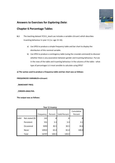
a) The syntax used to produce a frequency table and bar chart was as follows:
FREQUENCIES VARIABLES=s1truan1
/BARCHART FREQ
/ORDER=ANALYSIS.
The output was as follows:
Year 11 truancy
Frequency Percent Valid Percent
Cumulative
Percent
Valid Not stated (9) 141 .8 .8 .8
Persistent 551 3.3 3.3 4.1
Occasional 5093 30.5 30.5 34.6
Never 10922 65.4 65.4 100.0
Total 16707 100.0 100.0

) In order to produce a contingency table (Crosstab) of sex by truanting behaviour the following
syntax was used:
CROSSTABS
/TABLES=s1sex BY s1truan1
/FORMAT=AVALUE TABLES
/CELLS=COUNT ROW
/COUNT ROUND CELL.

The following table was produced:
Respondent's gender * Year 11 truancy Crosstabulation
Year 11 truancy
Not stated
(9) Persistent Occasional Never Total
Respondent's
gender
Male Count 71 219 2142 5032 7464
% within Respondent's
gender
1.0% 2.9% 28.7% 67.4% 100.0%
Female Count 70 332 2951 5890 9243
% within Respondent's
gender
.8% 3.6% 31.9% 63.7% 100.0%
Total Count 141 551 5093 10922 16707
% within Respondent's
gender
.8% 3.3% 30.5% 65.4% 100.0%
Row percentages are calculated so that it is possible to compare the percentage of boys who are
persistent truants and the percentage of girls who are persistent truants. This table suggests that
girls are more likely than boys to be truants.
6.2 The teaching dataset YCS11_teach.sav also includes a separate variable for mother and
father’s social position measured using NS‐SEC. The table below shows a contingency table
of mother’s social position by father’s social position.

Figure 6.19 SPSS output showing contingency table of mother’s social position by father’s social
position
dadsec father's grouped ns-sec * momsec mother's grouped ns-sec Crosstabulation
dadsec
father's
grouped
ns-sec
1.00 Large employers
and higher professionals
2.00 Lower professional
and higher technical
occupations
Count
% of Total
Count
% of Total
1.00 Large
employers
and higher
2.00 Lower
professional
and higher
technical
momsec mother's grouped ns-sec
3.00
Intermediate
4.00 Lower
supervisory
5.00 Semi
routine and
routine
professionals occupations occupations occupations occupations 6
90 298 184 38 157
1.5% 4.8% 3.0% .6% 2.5%
61 380 235 63 210
1.0% 6.1% 3.8% 1.0% 3.4%
Total
3.00 Intermediate
4.00 Lower supervisory
occupations
5.00 Semi routine and
routine occupations
6.00 Other
Count
% of Total
Count
% of Total
Count
% of Total
Count
% of Total
Count
% of Total
37 215 383 99 292
.6% 3.5% 6.2% 1.6% 4.7%
23 168 138 132 270
.4% 2.7% 2.2% 2.1% 4.4%
13 107 122 95 392
.2% 1.7% 2.0% 1.5% 6.3%
31 202 139 62 302
.5% 3.3% 2.2% 1.0% 4.9%
255 1370 1201 489 1623
4.1% 22.2% 19.4% 7.9% 26.2%
a) What percentage of mothers and fathers are in the same category of NS‐SEC?
The figure of 90 (1.5%) in the top left hand corner of the table indicates that there are 90 mothers
and fathers (from a total of 6184) who are both in the category ‘Large employers and higher
professionals’. Therefore by adding the percentages down the leading diagonal (1.5+ 6.1+6.2+
2.1+6.3+7.5) we obtain 29.7%. This is the percentage of mothers and fathers who are in the same
category of NS‐SEC.
b) What percentage of fathers are in a higher social class position
than their wives/partners and what percentage of mothers are in a
higher social class position than their husbands/partners?
In total 42.4% of fathers are in a higher social class position than their wives/partners and 27.7%
of mothers are in a higher social class than their husbands/partners. This assumes that we treat
the ‘other’ category as being in a lower social class position than the other categories.
c) Check that you can replicate the table using SPSS.

6.3 The following table is adapted from Fiegehan et al. (1977); the authors set out to investigate
both the causes of poverty and the type of social policy that would best alleviate it. In order
to discover whether household size had any effect on poverty, they re‐analysed some data
originally collected for the Family Expenditure Survey, and got a table something like that
shown in figure 6.20.
Figure 6.20
Household size by numbers in poverty
Number in household In poverty Not in poverty Total
1 259 991 1250
2 148 2159 2307
3 45 1319 1364
4 21 1272 1293
5 16 573 589
6 or more 21 324 345
Total 510 6638 7148
Construct two tables running the percentages both ways and say how each table might contribute
to understanding the relationship between poverty and household size. What advice would you give
to a policy‐maker about where to concentrate resources to alleviate poverty on the basis of these
figures?
Number in household Risk of
poverty
Accountability
for poverty
1 20.7 50.8
2 6.4 29.0
3 3.3 8.8
4 1.6 4.1
5 2.7 3.1
6 or more 6.1 4.1
Calculating row percentages provides the risk of poverty for each household size. For example the
risk of being in poverty if you are in a one‐person household is [(259/1250) x 100] because 259 out
of 1250 one‐person households are in poverty. This suggests that it is those in one‐person
households who are at greatest risk of being in poverty. In addition by calculating column
percentages we can see that those in one‐person households account for 50.8% of all households

that are in poverty. Policy makers would therefore be advised to focus resources on
one‐person households.
6.4 The NCDS teaching dataset NCDS_ExpData_teach.sav contains information on the social
class of cohort members at age 46 and the social class of their father when they were aged
16. Construct both an inflow and an outflow mobility table and discuss the results.
By calculating row percentages (with Father’s social class defining the rows) we get an ‘outflow’
table. This shows, for example that of those boys with a father in social class 1 at age 16, 19%
became professionals by age 46 compared with just 4.4% of boys with a manual father. In
contrast, by calculating the column percentages we create an inflow table and discover that 8.5%
of those who are currently in the professional group at age 46 come from a background with a
manual father in social class IV. Arguably the inflow table, with row percentages, gives a better
indication of the level of social mobility for those boys born in 1958. This is because it can be used
to look at the relative chances of boys with different social class backgrounds reaching the
Professional social class by age 46.

3P Social class
father,male
head (GRO
1970) at age 16 I Professional
II Managerialtechnical
(Current Job) Social Class at age 46
IIINM Skilled IIIM Skilled
non‐manual manual IV Partly skilled V Unskilled Others Total
I Count 69 195 48 31 17 2 1 363
% within 3P Social class
father,male head (GRO
1970) at age 16
19.0% 53.7% 13.2% 8.5% 4.7% .6% .3% 100.0%
II Count 116 674 242 139 93 17 3 1284
% within 3P Social class
father,male head (GRO
1970) at age 16
9.0% 52.5% 18.8% 10.8% 7.2% 1.3% .2% 100.0%
III non‐manual Count 41 277 132 107 46 4 3 610
% within 3P Social class
father,male head (GRO
1970) at age 16
6.7% 45.4% 21.6% 17.5% 7.5% .7% .5% 100.0%
III manual Count 88 901 558 559 280 63 1 2450
% within 3P Social class
father,male head (GRO
1970) at age 16
3.6% 36.8% 22.8% 22.8% 11.4% 2.6% .0% 100.0%
IV non‐manual Count 2 39 15 23 18 1 0 98
% within 3P Social class
father,male head (GRO
1970) at age 16
2.0% 39.8% 15.3% 23.5% 18.4% 1.0% .0% 100.0%
IV manual Count 30 239 130 140 117 28 2 686
% within 3P Social class
father,male head (GRO
1970) at age 16
4.4% 34.8% 19.0% 20.4% 17.1% 4.1% .3% 100.0%

V Count 3 76 46 54 43 15 0 237
% within 3P Social class
father,male head (GRO
1970) at age 16
1.3% 32.1% 19.4% 22.8% 18.1% 6.3% .0% 100.0%
Unclear Count 4 30 16 4 11 4 0 69
% within 3P Social class
father,male head (GRO
1970) at age 16
5.8% 43.5% 23.2% 5.8% 15.9% 5.8% .0% 100.0%
Total Count 353 2431 1187 1057 625 134 10 5797
% within 3P Social class
father,male head (GRO
1970) at age 16
6.1% 41.9% 20.5% 18.2% 10.8% 2.3% .2% 100.0%
(Current Job) Social Class at age 46
3P Social class
father,male head
(GRO 1970) at
age 16
I Professional
II Managerialtechnical
IIINM Skilled
non‐manual
IIIM Skilled
manual IV Partly skilled V Unskilled Others Total
I Count 69 195 48 31 17 2 1 363
% within (Current Job) Social
Class at age 46
19.5% 8.0% 4.0% 2.9% 2.7% 1.5% 10.0% 6.3%
II Count 116 674 242 139 93 17 3 1284
% within (Current Job) Social
Class at age 46
32.9% 27.7% 20.4% 13.2% 14.9% 12.7% 30.0% 22.1%
III non‐manual Count 41 277 132 107 46 4 3 610
% within (Current Job) Social
Class at age 46
11.6% 11.4% 11.1% 10.1% 7.4% 3.0% 30.0% 10.5%

III manual Count 88 901 558 559 280 63 1 2450
% within (Current Job) Social
Class at age 46
24.9% 37.1% 47.0% 52.9% 44.8% 47.0% 10.0% 42.3%
IV non‐manual Count 2 39 15 23 18 1 0 98
% within (Current Job) Social
Class at age 46
.6% 1.6% 1.3% 2.2% 2.9% .7% .0% 1.7%
IV manual Count 30 239 130 140 117 28 2 686
% within (Current Job) Social
Class at age 46
8.5% 9.8% 11.0% 13.2% 18.7% 20.9% 20.0% 11.8%
V Count 3 76 46 54 43 15 0 237
% within (Current Job) Social
Class at age 46
.8% 3.1% 3.9% 5.1% 6.9% 11.2% .0% 4.1%
Unclear Count 4 30 16 4 11 4 0 69
% within (Current Job) Social
Class at age 46
1.1% 1.2% 1.3% .4% 1.8% 3.0% .0% 1.2%
Total Count 353 2431 1187 1057 625 134 10 5797
% within (Current Job) Social
Class at age 46
100.0% 100.0% 100.0% 100.0% 100.0% 100.0% 100.0% 100.0%