Statistical power analyses using G*Power 3.1 - Psychologie ...

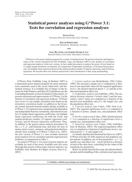
Behavior Research Methods 

2009, 41 (4), 1149-1160 

doi:10.3758/BRM.41.4.1149 

Statistical power analyses using G*Power 3.1: 

Tests for correlation and regression analyses 

Franz Fau l 

Christian-Albrechts-Universität, Kiel, Germany 

Edgar Erdfelder 

Universität Mannheim, Mannheim, Germany 

and 

Axel Buchner and Albert-Georg Lang 

Heinrich-Heine-Universität, Düsseldorf, Germany 

G*Power is a free power analysis program for a variety of statistical tests. We present extensions and improvements 

of the version introduced by Faul, Erdfelder, Lang, and Buchner (2007) in the domain of correlation 

and regression analyses. In the new version, we have added procedures to analyze the power of tests based on 

(1) single-sample tetrachoric correlations, (2) comparisons of dependent correlations, (3) bivariate linear regression, 

(4) multiple linear regression based on the random predictor model, (5) logistic regression, and (6) Poisson 

regression. We describe these new features and provide a brief introduction to their scope and handling. 

G*Power (Faul, Erdfelder, Lang, & Buchner, 2007) is 

a stand-alone power analysis program for many statistical 

tests commonly used in the social, behavioral, and biomedical 

sciences. It is available free of charge via the Internet 

for both Windows and Mac OS X platforms (see the 

Concluding Remarks section for details). In this article, we 

present extensions and improvements of G*Power 3 in the 

domain of correlation and regression analyses. G*Power 

now covers (1) one-sample correlation tests based on the 

tetrachoric correlation model, in addition to the bivariate 

normal and point biserial models already available in 

G*Power 3, (2) statistical tests comparing both dependent 

and independent Pearson correlations, and statistical tests 

for (3) simple linear regression coefficients, (4) multiple 

linear regression coefficients for both the fixed- and 

random-predictors models, (5) logistic regression coefficients, 

and (6) Poisson regression coefficients. Thus, 

in addition to the generic power analysis procedures for 

the z, t, F, χ 2 , and binomial tests, and those for tests of 

means, mean vectors, variances, and proportions that have 

already been available in G*Power 3 (Faul et al., 2007), 

the new version, G*Power 3.1, now includes statistical 

power analyses for six correlation and nine regression test 

problems, as summarized in Table 1. 

As usual in G*Power 3, five types of power analysis are 

available for each of the newly available tests (for more 

thorough discussions of these types of power analyses, see 

Erdfelder, Faul, Buchner, & Cüpper, in press; Faul et al., 

2007): 

1. A priori analysis (see Bredenkamp, 1969; Cohen, 

1988). The necessary sample size is computed as a function 

of user-specified values for the required significance 

level α, the desired statistical power 12β, and the to-bedetected 

population effect size. 

2. Compromise analysis (see Erdfelder, 1984). The statistical 

decision criterion (“critical value”) and the associated 

α and β values are computed as a function of the 

desired error probability ratio β/α, the sample size, and 

the population effect size. 

3. Criterion analysis (see Cohen, 1988; Faul et al., 

2007). The required significance level α is computed as 

a function of power, sample size, and population effect 

size. 

4. Post hoc analysis (see Cohen, 1988). Statistical power 

12β is computed as a function of significance level α, 

sample size, and population effect size. 

5. Sensitivity analysis (see Cohen, 1988; Erdfelder, 

Faul, & Buchner, 2005). The required population effect 

size is computed as a function of significance level α, statistical 

power 12β, and sample size. 

As already detailed and illustrated by Faul et al. (2007), 

G*Power provides for both numerical and graphical output 

options. In addition, any of four parameters—α, 12β, 

sample size, and effect size—can be plotted as a function 

of each of the other three, controlling for the values of the 

remaining two parameters. 

Below, we briefly describe the scope, the statistical background, 

and the handling of the correlation and regression 

E. Erdfelder, erdfelder@psychologie.uni-mannheim.de 

1149 © 2009 The Psychonomic Society, Inc.

1150 Fau l, Erdfelder, Buchner, and Lang 

Table 1 

Summary of the Correlation and 

Regression Test Problems Covered by G*Power 3.1 

Correlation Problems Referring to One Correlation 

Comparison of a correlation ρ with a constant ρ 0 (bivariate normal model) 

Comparison of a correlation ρ with 0 (point biserial model) 

Comparison of a correlation ρ with a constant ρ 0 (tetrachoric correlation model) 

Correlation Problems Referring to Two Correlations 

Comparison of two dependent correlations ρ jk and ρ jh (common index) 

Comparison of two dependent correlations ρ jk and ρ hm (no common index) 

Comparison of two independent correlations ρ 1 and ρ 2 (two samples) 

Linear Regression Problems, One Predictor (Simple Linear Regression) 

Comparison of a slope b with a constant b 0 

Comparison of two independent intercepts a 1 and a 2 (two samples) 

Comparison of two independent slopes b 1 and b 2 (two samples) 

Linear Regression Problems, Several Predictors (Multiple Linear Regression) 

Deviation of a squared multiple correlation ρ 2 from zero (F test, fixed model) 

Deviation of a subset of linear regression coefficients from zero (F test, fixed model) 

Deviation of a single linear regression coefficient b j from zero (t test, fixed model) 

Deviation of a squared multiple correlation ρ 2 from constant (random model) 

Generalized Linear Regression Problems 

Logistic regression 

Poisson regression 

power analysis procedures that are new in G*Power 3.1. 

Further technical details about the tests described here, 

as well as information on those tests in Table 1 that were 

already available in the previous version of G*Power, can 

be found on the G*Power Web site (see the Concluding 

Remarks section). We describe the new tests in the order 

shown in Table 1 (omitting the procedures previously described 

by Faul et al., 2007), which corresponds to their 

order in the “Tests Correlation and regression” dropdown 

menu of G*Power 3.1 (see Figure 1). 

1. The Tetrachoric Correlation Model 

The “Correlation: Tetrachoric model” procedure refers 

to samples of two dichotomous random variables X and Y 

as typically represented by 2 3 2 contingency tables. The 

tetrachoric correlation model is based on the assumption 

that these variables arise from dichotomizing each of two 

standardized continuous random variables following a bivariate 

normal distribution with correlation ρ in the underlying 

population. This latent correlation ρ is called the tetrachoric 

correlation. G*Power 3.1 provides power analysis 

procedures for tests of H 0 : ρ 5 ρ 0 against H 1 : ρ ρ 0 (or 

the corresponding one-tailed hypotheses) based on (1) a 

precise method developed by Brown and Benedetti (1977) 

and (2) an approximation suggested by Bonett and Price 

(2005). The procedure refers to the Wald z statistic W 5 

(r 2 ρ 0 )/se 0 (r), where se 0 (r) is the standard error of the 

sample tetrachoric correlation r under H 0 : ρ 5 ρ 0 . W follows 

a standard normal distribution under H 0 . 

Effect size measure. The tetrachoric correlation under 

H 1 , ρ 1 , serves as an effect size measure. Using the effect 

size drawer (i.e., a subordinate window that slides out 

from the main window after clicking on the “Determine” 

button), it can be calculated from the four probabilities of 

the 2 3 2 contingency tables that define the joint distribution 

of X and Y. To our knowledge, effect size conventions 

have not been defined for tetrachoric correlations. However, 

Cohen’s (1988) conventions for correlations in the 

framework of the bivariate normal model may serve as 

rough reference points. 

Options. Clicking on the “Options” button opens a 

window in which users may choose between the exact approach 

of Brown and Benedetti (1977) (default option) or 

an approximation suggested by Bonett and Price (2005). 

Input and output parameters. Irrespective of the 

method chosen in the options window, the power of the tetrachoric 

correlation z test depends not only on the values of 

ρ under H 0 and H 1 but also on the marginal distributions of 

X and Y. For post hoc power analyses, one therefore needs 

to provide the following input in the lower left field of the 

main window: The number of tails of the test (“Tail(s)”: 

one vs. two), the tetrachoric correlation under H 1 (“H1 corr 

ρ”), the α error probability, the “Total sample size” N, the 

tetrachoric correlation under H 0 (“H0 corr ρ”), and the 

marginal probabilities of X 5 1 (“Marginal prob x”) and 

Y 5 1 (“Marginal prob y”)—that is, the proportions of values 

exceeding the two criteria used for dichotomization. 

The output parameters include the “Critical z” required 

for deciding between H 0 and H 1 and the “Power (12β err 

prob).” In addition, critical values for the sample tetrachoric 

correlation r (“Critical r upr” and “Critical r lwr”) 

and the standard error se(r) of r (“Std err r”) under H 0 are 

also provided. Hence, if the Wald z statistic W 5 (r 2 ρ 0 )/ 

se(r) is unavailable, G*Power users can base their statistical 

decision on the sample tetrachoric r directly. For a twotailed 

test, H 0 is retained whenever r is not less than “Critical 

r lwr” and not larger than “Critical r upr”; otherwise H 0 

is rejected. For one-tailed tests, in contrast, “Critical r lwr” 

and “Critical r upr” are identical; H 0 is rejected if and only 

if r exceeds this critical value. 

Illustrative example. Bonett and Price (2005, Example 

1) reported the following “yes” (5 1) and “no” (5 2)

G*Pow e r 3.1: Correlation and Regression 1151 

Figure 1. The main window of G*Power, showing the contents of the “Tests Correlation and regression” drop-down menu. 

answer frequencies of 930 respondents to two questions 

in a personality inventory: f 11 5 203, f 12 5 186, f 21 5 

167, f 22 5 374. The option “From C.I. calculated from 

observed freq” in the effect size drawer offers the possibility 

to use the (12α) confidence interval for the sample 

tetrachoric correlation r as a guideline for the choice of 

the correlation ρ under H 1 . To use this option, we insert 

the observed frequencies in the corresponding fields. If 

we assume, for example, that the population tetrachoric 

correlation under H 1 matches the sample tetrachoric correlation 

r, we should choose the center of the C.I. (i.e., the 

correlation coefficient estimated from the data) as “H1 

corr ρ” and press “Calculate.” Using the exact calculation 

method, this results in a sample tetrachoric correlation 

r 5 .334 and marginal proportions p x 5 .602 and p y 5 

.582. We then click on “Calculate and transfer to main 

window” in the effect size drawer. This copies the calculated 

parameters to the corresponding input fields in the 

main window. 

For a replication study, say we want to know the sample 

size required for detecting deviations from H 0 : ρ 5 0 consistent 

with the above H 1 scenario using a one-tailed test


and a power (12β) 5 .95, given α 5 .05. If we choose the 

a priori type of power analysis and insert the corresponding 

input parameters, clicking on “Calculate” provides 

us with the result “Total sample size” 5 229, along with 

“Critical z” 5 1.644854 for the z test based on the exact 

method of Brown and Benedetti (1977). 

2. Correlation Problems Referring 

to Two Dependent Correlations 

This section refers to z tests comparing two dependent 

Pearson correlations that either share (Section 2.1) or do 

not share (Section 2.2) a common index. 

2.1. Comparison of Two Dependent 

Correlations ρ ab and ρ ac (Common Index) 

The “Correlations: Two dependent Pearson r’s (common 

index)” procedure provides power analyses for tests of the 

null hypothesis that two dependent Pearson correlations 

ρ ab and ρ ac are identical (H 0 : ρ ab 5 ρ ac ). Two correlations 

are dependent if they are defined for the same population. 

Correspondingly, their sample estimates, r ab and r ac , are 

observed for the same sample of N observations of three 

continuous random variables X a , X b , and X c . The two correlations 

share a common index because one of the three 

random variables, X a , is involved in both correlations. 

Assuming that X a , X b , and X c are multivariate normally 

distributed, Steiger’s (1980, Equation 11) Z1 * statistic follows 

a standard normal distribution under H 0 (see also 

Dunn & Clark, 1969). G*Power’s power calculations for 

dependent correlations sharing a common index refer to 

this test. 

Effect size measure. To specify the effect size, both 

correlations ρ ab and ρ ac are required as input parameters. 

Alternatively, clicking on “Determine” opens the effect 

size drawer, which can be used to compute ρ ac from ρ ab 

and Cohen’s (1988, p. 109) effect size measure q, the difference 

between the Fisher r-to-z transforms of ρ ab and 

ρ ac . Cohen suggested calling effects of sizes q 5 .1, .3, 

and .5 “small,” “medium,” and “large,” respectively. Note, 

however, that Cohen developed his q effect size conventions 

for comparisons between independent correlations 

in different populations. Depending on the size of the third 

correlation involved, ρ bc , a specific value of q can have 

very different meanings, resulting in huge effects on statistical 

power (see the example below). As a consequence, 

ρ bc is required as a further input parameter. 

Input and output parameters. Apart from the number 

of “Tail(s)” of the z test, the post hoc power analysis 

procedure requires ρ ac (i.e., “H1 Corr ρ_ac”), the significance 

level “α err prob,” the “Sample Size” N, and the two 

remaining correlations “H0 Corr ρ_ab” and “Corr ρ_bc” 

as input parameters in the lower left field of the main window. 

To the right, the “Critical z” criterion value for the 

z test and the “Power (12β err prob)” are displayed as 

output parameters. 

Illustrative example. Tsujimoto, Kuwajima, and 

Sawaguchi (2007, p. 34, Table 2) studied correlations 

between age and several continuous measures of working 

memory and executive functioning in children. In 

8- to 9-year-olds, they found age correlations of .27 and 

.17 with visuospatial working memory (VWM) and auditory 

working memory (AWM), respectively. The correlation 

of the two working memory measures was 

r(VWM, AWM) 5 .17. Assume we would like to know 

whether VWM is more strongly correlated with age 

than AWM in the underlying population. In other words, 

H 0 : ρ(Age, VWM) # ρ(Age, AWM) is tested against the 

one-tailed H 1 : ρ(Age, VWM) . ρ(Age, AWM). Assuming 

that the true population correlations correspond to the 

results reported by Tsujimoto et al., what is the sample 

size required to detect such a correlation difference with 

a power of 12β 5 .95 and α 5 .05? To find the answer, 

we choose the a priori type of power analysis along 

with “Correlations: Two dependent Pearson r’s (common 

index)” and insert the above parameters (ρ ac 5 .27, 

ρ ab 5 .17, ρ bc 5 .17) in the corresponding input fields. 

Clicking on “Calculate” provides us with N 5 1,663 as 

the required sample size. Note that this N would drop to 

N 5 408 if we assumed ρ(VWM, AWM) 5 .80 rather than 

ρ(VWM, AWM) 5 .17, other parameters being equal. Obviously, 

the third correlation ρ bc has a strong impact on 

statistical power, although it does not affect whether H 0 or 

H 1 holds in the underlying population. 

2.2. Comparison of Two Dependent 

Correlations ρ ab and ρ cd (No Common Index) 

The “Correlations: Two dependent Pearson r’s (no common 

index)” procedure is very similar to the procedure 

described in the preceding section. The single difference is 

that H 0 : ρ ab 5 ρ cd is now contrasted against H 1 : ρ ab ρ cd ; 

that is, the two dependent correlations here do not share 

a common index. G*Power’s power analysis procedures 

for this scenario refer to Steiger’s (1980, Equation 12) 

Z2 * test statistic. As with Z1 * , which is actually a special 

case of Z2 * , the Z2 * statistic is asymptotically z distributed 

under H 0 given a multivariate normal distribution of the 

four random variables X a , X b , X c , and X d involved in ρ ab 

and ρ cd (see also Dunn & Clark, 1969). 

Effect size measure. The effect size specification is 

identical to that for “Correlations: Two dependent Pearson 

r’s (common index),” except that all six pairwise correlations 

of the random variables X a , X b , X c , and X d under H 1 

need to be specified here. As a consequence, ρ ac , ρ ad , ρ bc , 

and ρ bd are required as input parameters in addition to ρ ab 

and ρ cd . 

Input and output parameters. By implication, 

the input parameters include “Corr ρ_ac,” “Corr ρ_ad,” 

“Corr ρ_bc,” and “Corr ρ_bd” in addition to the correlations 

“H1 corr ρ_cd” and “H0 corr ρ_ab” to which the 

hypotheses refer. There are no other differences from the 

procedure described in the previous section. 

Illustrative example. Nosek and Smyth (2007) reported 

a multitrait–multimethod validation using two 

attitude measurement methods, the Implicit Association 

Test (IAT) and self-report (SR). IAT and SR measures 

of attitudes toward Democrats versus Republicans (DR) 

were correlated at r(IAT-DR, SR-DR) 5 .51 5 r cd . In 

contrast, when measuring attitudes toward whites versus 

blacks (WB), the correlation between both methods was 

only r(IAT-WB, SR-WB) 5 .12 5 r ab , probably because


SR measures of attitudes toward blacks are more strongly 

biased by social desirability influences. Assuming that 

(1) these correlations correspond to the true population correlations 

under H 1 and (2) the other four between-attitude 

correlations ρ(IAT-WB, IAT-DR), ρ(IAT-WB, SR-DR), 

ρ(SR-WB, IAT-DR), and ρ(SR-WB, SR-DR) are zero, 

how large must the sample be to make sure that this deviation 

from H 0 : ρ(IAT-DR, SR-DR) 5 ρ(IAT-WB, SR-WB) 

is detected with a power of 12β 5 .95 using a one-tailed 

test and α 5 .05? An a priori power analysis for “Correlations: 

Two dependent Pearson r’s (no common index)” 

computes N 5 114 as the required sample size. 

The assumption that the four additional correlations 

are zero is tantamount to assuming that the two correlations 

under test are statistically independent (thus, the 

procedure in G*Power for independent correlations could 

alternatively have been used). If we instead assume that 

ρ(IAT-WB, IAT-DR) 5 ρ ac 5 .6 and ρ(SR-WB, SR-DR) 5 

ρ bd 5 .7, we arrive at a considerably lower sample size of 

N 5 56. If our resources were sufficient for recruiting not 

more than N 5 40 participants and we wanted to make 

sure that the “β/α ratio” equals 1 (i.e., balanced error risks 

with α 5 β), a compromise power analysis for the latter 

case computes “Critical z” 5 1.385675 as the optimal 

statistical decision criterion, corresponding to α 5 β 5 

.082923. 

3. Linear Regression Problems, 

One Predictor (Simple Linear Regression) 

This section summarizes power analysis procedures 

addressing regression coefficients in the bivariate linear 

standard model Y i 5 a 1 b·X i 1 E i , where Y i and X i represent 

the criterion and the predictor variable, respectively, 

a and b the regression coefficients of interest, and E i an 

error term that is independently and identically distributed 

and follows a normal distribution with expectation 0 

and homogeneous variance σ 2 for each observation unit i. 

Section 3.1 describes a one-sample procedure for tests addressing 

b, whereas Sections 3.2 and 3.3 refer to hypotheses 

on differences in a and b between two different underlying 

populations. Formally, the tests considered here 

are special cases of the multiple linear regression procedures 

described in Section 4. However, the procedures for 

the special case provide a more convenient interface that 

may be easier to use and interpret if users are interested 

in bivariate regression problems only (see also Dupont & 

Plummer, 1998). 

3.1. Comparison of a Slope b With a Constant b 0 

The “Linear bivariate regression: One group, size of 

slope” procedure computes the power of the t test of 

H 0 : b 5 b 0 against H 1 : b b 0 , where b 0 is any real-valued 

constant. Note that this test is equivalent to the standard 

bivariate regression t test of H 0 : b * 5 0 against H 1 : b * 0 

if we refer to the modified model Y i 

* 5 a 1 b *·X i 1 E i , 

with Y i 

* :5 Y i 2 b 0·X i (Rindskopf, 1984). Hence, power 

could also be assessed by referring to the standard regression 

t test (or global F test) using Y * rather than Y as a 

criterion variable. The main advantage of the “Linear bivariate 

regression: One group, size of slope” procedure 

is that power can be computed as a function of the slope 

values under H 0 and under H 1 directly (Dupont & Plummer, 

1998). 

Effect size measure. The slope b assumed under H 1 , 

labeled “Slope H1,” is used as the effect size measure. Note 

that the power does not depend only on the difference between 

“Slope H1” and “Slope H0,” the latter of which is the 

value b 5 b 0 specified by H 0 . The population standard deviations 

of the predictor and criterion values, “Std dev σ_x” 

and “Std dev σ_y,” are also required. The effect size drawer 

can be used to calculate “Slope H1” from other basic parameters 

such as the correlation ρ assumed under H 1 . 

Input and output parameters. The number of 

“Tail(s)” of the t test, “Slope H1,” “α err prob,” “Total 

sample size,” “Slope H0,” and the standard deviations 

(“Std dev σ_x” and “Std dev σ_y”) need to be specified 

as input parameters for a post hoc power analysis. “Power 

(12β err prob)” is displayed as an output parameter, in 

addition to the “Critical t” decision criterion and the parameters 

defining the noncentral t distribution implied by 

H 1 (the noncentrality parameter δ and the df of the test). 

Illustrative example. Assume that we would like to 

assess whether the standardized regression coefficient β 

of a bivariate linear regression of Y on X is consistent with 

H 0 : β $ .40 or H 1 : β , .40. Assuming that β 5 .20 actually 

holds in the underlying population, how large must the 

sample size N of X–Y pairs be to obtain a power of 12β 5 

.95 given α 5 .05? After choosing “Linear bivariate regression: 

One group, size of slope” and the a priori type 

of power analysis, we specify the above input parameters, 

making sure that “Tail(s)” 5 one, “Slope H1” 5 .20, “Slope 

H0” 5 .40, and “Std dev σ_x” 5 “Std dev σ_y” 5 1, because 

we want to refer to regression coefficients for standardized 

variables. Clicking on “Calculate” provides us 

with the result “Total sample size” 5 262. 

3.2. Comparison of Two Independent 

Intercepts a 1 and a 2 (Two Samples) 

The “Linear bivariate regression: Two groups, difference 

between intercepts” procedure is based on the assumption 

that the standard bivariate linear model described above 

holds within each of two different populations with the 

same slope b and possibly different intercepts a 1 and a 2 . It 

computes the power of the two-tailed t test of H 0 : a 1 5 a 2 

against H 1 : a 1 a 2 and for the corresponding one-tailed 

t test, as described in Armitage, Berry, and Matthews 

(2002, ch. 11). 

Effect size measure. The absolute value of the difference 

between the intercepts, |D intercept| 5 |a 1 2 a 2 |, is 

used as an effect size measure. In addition to |D intercept|, 

the significance level α, and the sizes n 1 and n 2 of the two 

samples, the power depends on the means and standard 

deviations of the criterion and the predictor variable. 

Input and output parameters. The number of 

“Tail(s)” of the t test, the effect size “|D intercept|,” the 

“α err prob,” the sample sizes in both groups, the standard 

deviation of the error variable E ij (“Std dev residual σ”), 

the means (“Mean m_x1,” “Mean m_x2”), and the standard 

deviations (“Std dev σ_x1,” “Std dev σ_x2”) are required 

as input parameters for a “Post hoc” power analysis. The


“Power (12β err prob)” is displayed as an output parameter 

in addition to the “Critical t” decision criterion and 

the parameters defining the noncentral t distribution implied 

by H 1 (the noncentrality parameter δ and the df of 

the test). 

3.3. Comparison of Two Independent 

Slopes b 1 and b 2 (Two Samples) 

The linear model used in the previous two sections also 

underlies the “Linear bivariate regression: Two groups, differences 

between slopes” procedure. Two independent samples 

are assumed to be drawn from two different populations, 

each consistent with the model Y ij 5 a j 1 b j·X i 1 E i , 

where Y ij , X ij , and E ij respectively represent the criterion, 

the predictor, and the normally distributed error variable 

for observation unit i in population j. Parameters a j and b j 

denote the regression coefficients in population j, j 5 1, 2. 

The procedure provides power analyses for two-tailed t tests 

of the null hypothesis that the slopes in the two populations 

are equal (H 0 : b 1 5 b 2 ) versus different (H 1 : b 1 b 2 ) and 

for the corresponding one-tailed t test (Armitage et al., 

2002, ch. 11, Equations 11.18–11.20). 

Effect size measure. The absolute difference between 

slopes, |D slope| 5 |b 1 2 b 2 |, is used as an effect size measure. 

Statistical power depends not only on |D slope|, α, and 

the two sample sizes n 1 and n 2 . Specifically, the standard 

deviations of the error variable E ij (“Std dev residual σ”), 

the predictor variable (“Std dev σ_X”), and the criterion 

variable (“Std dev σ_Y”) in both groups are required to 

fully specify the effect size. 

Input and output parameters. The input and output 

parameters are similar to those for the two procedures described 

in Sections 3.1 and 3.2. In addition to |D slope| and 

the standard deviations, the number of “Tail(s)” of the test, 

the “α err prob,” and the two sample sizes are required in 

the Input Parameters fields for the post hoc type of power 

analysis. In the Output Parameters fields, the “Noncentrality 

parameter δ” of the t distribution under H 1 , the decision 

criterion (“Critical t”), the degrees of freedom of the 

t test (“Df ”), and the “Power (12β err prob)” implied by 

the input parameters are provided. 

Illustrative application. Perugini, O’Gorman, and 

Prestwich (2007, Study 1) hypothesized that the criterion 

validity of the IAT depends on the degree of self-activation 

in the test situation. To test this hypothesis, they asked 60 

participants to circle certain words while reading a short 

story printed on a sheet of paper. Half of the participants 

were asked to circle the words “the” and “a” (control condition), 

whereas the remaining 30 participants were asked 

to circle “I,” “me,” “my,” and “myself ” (self-activation 

condition). Subsequently, attitudes toward alcohol versus 

soft drinks were measured using the IAT (predictor X ). 

In addition, actual alcohol consumption rate was assessed 

using the self-report (criterion Y ). Consistent with their 

hypothesis, they found standardized Y–X regression coefficients 

of β 5 .48 and β 5 2.09 in the self-activation and 

control conditions, respectively. Assuming that (1) these 

coefficients correspond to the actual coefficients under H 1 

in the underlying populations and (2) the error standard deviation 

is .80, how large is the power of the one-tailed t test 

of H 0 : b 1 # b 2 against H 1 : b 1 . b 2 , given α 5 .05? To answer 

this question, we select “Linear bivariate regression: 

Two groups, difference between slopes” along with the 

post hoc type of power analysis. We then provide the appropriate 

input parameters [“Tail(s)” 5 one, “|D slope|” 5 

.57, “α error prob” 5 .05, “Sample size group 1” 5 

“ Sample size group 2” 5 30, “Std dev. residual σ” 5 .80, 

and “Std dev σ_X1” 5 “Std dev σ_X2” 5 1] and click 

on “ Calculate.” We obtain “Power (12β err prob)” 5 

.860165. 

4. Linear Regression Problems, Several 

Predictors (Multiple Linear Regression) 

In multiple linear regression, the linear relation between 

a criterion variable Y and m predictors X 5 (X 1 , . . . , X m ) 

is studied. G*Power 3.1 now provides power analysis procedures 

for both the conditional (or fixed-predictors) and 

the unconditional (or random-predictors) models of multiple 

regression (Gatsonis & Sampson, 1989; Sampson, 

1974). In the fixed-predictors model underlying previous 

versions of G*Power, the predictors X are assumed to be 

fixed and known. In the random-predictors model, by contrast, 

they are assumed to be random variables with values 

sampled from an underlying multivariate normal distribution. 

Whereas the fixed-predictors model is often more 

appropriate in experimental research (where known predictor 

values are typically assigned to participants by an 

experimenter), the random-predictors model more closely 

resembles the design of observational studies (where participants 

and their associated predictor values are sampled 

from an underlying population). The test procedures 

and the maximum likelihood estimates of the regression 

weights are identical for both models. However, the models 

differ with respect to statistical power. 

Sections 4.1, 4.2, and 4.3 describe procedures related 

to F and t tests in the fixed-predictors model of multiple 

linear regression (cf. Cohen, 1988, ch. 9), whereas Section 

4.4 describes the procedure for the random-predictors 

model. The procedures for the fixed-predictors model are 

based on the general linear model (GLM), which includes 

the bivariate linear model described in Sections 3.1–3.3 

as a special case (Cohen, Cohen, West, & Aiken, 2003). 

In other words, the following procedures, unlike those 

in the previous section, have the advantage that they are 

not limited to a single predictor variable. However, their 

disadvantage is that effect size specifications cannot be 

made in terms of regression coefficients under H 0 and H 1 

directly. Rather, variance proportions, or ratios of variance 

proportions, are used to define H 0 and H 1 (cf. Cohen, 1988, 

ch. 9). For this reason, we decided to include both bivariate 

and multiple linear regression procedures in G*Power 3.1. 

The latter set of procedures is recommended whenever statistical 

hypotheses are defined in terms of proportions of 

explained variance or whenever they can easily be transformed 

into hypotheses referring to such proportions. 

4.1. Deviation of a Squared Multiple Correlation 

ρ 2 From Zero (Fixed Model) 

The “Linear multiple regression: Fixed model, R 2 deviation 

from zero” procedure provides power analyses for


omnibus (or “global”) F tests of the null hypothesis that 

the squared multiple correlation between a criterion variable 

Y and a set of m predictor variables X 1 , X 2 , . . . , X m is 

zero in the underlying population (H 0 : ρY.X1,...,Xm 2 5 0) versus 

larger than zero (H 1 : ρY.X1,...,Xm 2 . 0). Note that the former 

hypothesis is equivalent to the hypothesis that all m regression 

coefficients of the predictors are zero (H 0 : b 1 5 

b 2 5 . . . 5 b m 5 0). By implication, the omnibus F test 

can also be used to test fully specified linear models of the 

type Y i 5 b 0 1 c 1·X 1i 1 . . . 1 c m·X mi 1 E i , where c 1 , . . . , 

c m are user-specified real-valued constants defining H 0 . 

To test this fully specified model, simply define a new 

criterion variable Y * i 

:5 Y i 2 c 1·X 1i 2 . . . 2 c m·X mi and 

perform a multiple regression of Y * on the m predictors X 1 

to X m . H 0 holds if and only if ρY*.X1,...,Xm 2 5 0—that is, if all 

regression coefficients are zero in the transformed regression 

equation pertaining to Y * (see Rindskopf, 1984). 

Effect size measure. Cohen’s f 2 , the ratio of explained 

variance and error variance, serves as the effect size measure 

(Cohen, 1988, ch. 9). Using the effect size drawer, f 2 

can be calculated directly from the squared multiple correlation 

ρY.X1,...,Xm 2 in the underlying population. For omnibus 

F tests, the relation between f 2 and ρY.X1,...,Xm 2 is simply 

given by f 2 5 ρY.X1,...,Xm 2 / (1 2 ρ2 Y.X1,...,Xm 

). According to 

Cohen (ch. 9), f 2 values of .02, .15, and .35 can be called 

“small,” “medium,” and “large” effects, respectively. Alternatively, 

one may compute f 2 by specifying a vector 

u of correlations between Y and the predictors X i along 

with the (m 3 m) matrix B of intercorrelations among the 

predictors. Given u and B, it is easy to derive ρY.X1,...,Xm 2 5 

u T B 21 u and, via the relation between f 2 and ρY.X1,...,Xm 2 described 

above, also f 2 . 

Input and output parameters. The post hoc power 

analysis procedure requires the population “Effect size f 2 ,” 

the “α err prob,” the “Total sample size” N, and the “Total 

number of predictors” m in the regression model as input 

parameters. It provides as output parameters the “Noncentrality 

parameter λ” of the F distribution under H 1 , the 

decision criterion (“Critical F”), the degrees of freedom 

(“Numerator df,” “Denominator df ”), and the power of 

the omnibus F test [“Power (12β err prob)”]. 

Illustrative example. Given three predictor variables 

X 1 , X 2 , and X 3 , presumably correlated to Y with ρ 1 5 .3, 

ρ 2 5 2.1, and ρ 3 5 .7, and with pairwise correlations of 

ρ 13 5 .4 and ρ 12 5 ρ 23 5 0, we first determine the effect 

size f 2 . Inserting b 5 (.3, 2.1, .7) and the intercorrelation 

matrix of the predictors in the corresponding input dialog 

in G*Power’s effect size drawer, we find that ρY.X1,...,Xm 2 5 .5 

and f 2 5 1. The results of an a priori analysis with this effect 

size reveals that we need a sample size of N 5 22 to achieve 

a power of .95 in a test based on α 5 .05. 

4.2. Deviation of a Subset of Linear Regression 

Coefficients From Zero (Fixed Model) 

Like the previous procedure, this procedure is based on 

the GLM, but this one considers the case of two Predictor 

Sets A (including X 1 , . . . , X k ) and B (including X k11 , . . . , 

X m ) that define the full model with m predictors. The 

“Linear multiple regression: Fixed model, R 2 increase” 

procedure provides power analyses for the special F test of 

H 0 : ρY.X1,...,Xm 2 5 ρ2 Y.X1,...,Xk 

(i.e., Set B does not increase the 

proportion of explained variance) versus H 1 : ρY.X1,...,Xm 2 . 

ρY.X1,...,Xk 2 (i.e., Set B increases the proportion of explained 

variance). Note that H 0 is tantamount to claiming that all 

m2k regression coefficients of Set B are zero. 

As shown by Rindskopf (1984), special F tests can 

also be used to assess various constraints on regression 

coefficients in linear models. For example, if Y i 5 b 0 1 

b 1·X 1i 1 . . . 1 b m·X mi 1 E i is the full linear model and 

Y i 5 b 0 1 b·X 1i 1 . . . 1 b·X mi 1 E i is a restricted H 0 

model claiming that all m regression coefficients are equal 

(H 0 : b 1 5 b 2 5 . . . 5 b m 5 b), we can define a new predictor 

variable X i 

:5 X 1i 1 X 2i 1 . . . 1 X mi and consider the 

restricted model Y i 5 b 0 1 b·X i 1 E i . Because this model 

is equivalent to the H 0 model, we can compare ρY.X1,...,Xm 

2 

and ρY.X 2 with a special F test to test H 0. 

Effect size measure. Cohen’s (1988) f 2 is again used 

as an effect size measure. However, here we are interested 

in the proportion of variance explained by predictors from 

Set B only, so that f 2 5 (ρY.X1,...,Xm 2 2 ρ2 Y.X1,...,Xk ) / (1 2 

ρY.X1,...,Xm 2 ) serves as an effect size measure. The effect size 

drawer can be used to calculate f 2 from the variance explained 

by Set B (i.e., ρY.X1,...,Xm 2 2 ρ2 Y.X1,...,Xk 

) and the error 

variance (i.e., 1 2 ρY.X1,...,Xm 2 ). Alternatively, f 2 can also be 

computed as a function of the partial correlation squared 

of Set B predictors (Cohen, 1988, ch. 9). 

Cohen (1988) suggested the same effect size conventions 

as in the case of global F tests (see Section 4.1). 

However, we believe that researchers should reflect the 

fact that a certain effect size, say f 2 5 .15, may have very 

different substantive meanings depending on the proportion 

of variance explained by Set A (i.e., ρY.X1,...,Xk 2 ). 

Input and output parameters. The inputs and outputs 

match those of the “Linear multiple regression: 

Fixed model, R 2 deviation from zero” procedure (see Section 

4.1), with the exception that the “Number of tested 

predictors” :5 m 2 k—that is, the number of predictors in 

Set B—is required as an additional input parameter. 

Illustrative example. In Section 3.3, we presented a 

power analysis for differences in regression slopes as 

analyzed by Perugini et al. (2007, Study 1). Multiple 

linear regression provides an alternative method to address 

the same problem. In addition to the self-report of 

alcohol use (criterion Y ) and the IAT attitude measure 

(predictor X ), two additional predictors are required 

for this purpose: a binary dummy variable G representing 

the experimental condition (G 5 0, control group; 

G 5 1, self-activation group) and, most importantly, a 

product variable G·X representing the interaction of the 

IAT measure and the experimental conditional. Differences 

in Y–X regression slopes in the two groups will 

show up as a significant effect of the G·X interaction in 

a regression model using Y as the criterion and X, G, and 

G·X as m 5 3 predictors. 

Given a total of N 5 60 participants (30 in each group), 

α 5 .05, and a medium size f 2 5 .15 of the interaction effect 

in the underlying population, how large is the power 

of the special F test assessing the increase in explained 

variance due to the interaction? To answer this question, 

we choose the post hoc power analysis in the “Linear mul-


tiple regression: Fixed model, R 2 increase” procedure. In 

addition to “Effect size f 2 ” 5 .15, “α err prob” 5 .05, and 

“Total sample size” 5 60, we specify “Number of tested 

predictors” 5 1 and “Total number of predictors” 5 3 

as input parameters, because we have m 5 3 predictors 

in the full model and only one of these predictors captures 

the effect of interest—namely, the interaction effect. 

Clicking on “Calculate” provides us with the result 

“Power (12β err prob)” 5 .838477. 

4.3. Deviation of a Single Linear Regression 

Coefficient b j From Zero (t Test, Fixed Model) 

Special F tests assessing effects of a single predictor 

X j in multiple regression models (hence, numerator 

df 5 1) are equivalent to two-tailed t tests of H 0 : b j 5 0. 

The “Linear multiple regression: Fixed model, single regression 

coefficient” procedure has been designed for this 

situation. The main reason for including this procedure 

in G*Power 3.1 is that t tests for single regression coefficients 

can take the form of one-tailed tests of, for example, 

H 0 : b j # 0 versus H 1 : b j . 0. Power analyses for 

one-tailed tests can be done most conveniently with the 

“Linear multiple regression: Fixed model, single regression 

coefficient” t test procedure. 

Effect size measures, input and output parameters. 

Because two-tailed regression t tests are special 

cases of the special F tests described in Section 4.2, the 

effect size measure and the input and output parameters 

are largely the same for both procedures. One exception is 

that “Numerator df ” is not required as an input parameter 

for t tests. Also, the number of “Tail(s)” of the test (one 

vs. two) is required as an additional input parameter in the 

t test procedure. 

Illustrative application. See the example described in 

Section 4.2. For the reasons outlined above, we would obtain 

the same power results if we were to analyze the same 

input parameters using the “Linear multiple regression: 

Fixed model, single regression coefficient” procedure 

with “Tail(s)” 5 two. In contrast, if we were to choose 

“Tail(s)” 5 one and keep the other parameters unchanged, 

the power would increase to .906347. 

4.4. Deviation of Multiple Correlation 

Squared ρ 2 From Constant (Random Model) 

The random-predictors model of multiple linear regression 

is based on the assumption that (Y, X 1 , . . . , X m ) are 

random variables with a joint multivariate normal distribution. 

Sampson (1974) showed that choice of the fixed 

or the random model has no bearing on the test of significance 

or on the estimation of the regression weights. 

However, the choice of model affects the power of the 

test. Several programs exist that can be used to assess 

the power for random-model tests (e.g., Dunlap, Xin, & 

Myers, 2004; Mendoza & Stafford, 2001; Shieh & Kung, 

2007; Steiger & Fouladi, 1992). However, these programs 

either rely on other software packages (Mathematica, 

Excel) or provide only a rather inflexible user interface. 

The procedures implemented in G*Power use the exact 

sampling distribution of the squared multiple correlation 

coefficient (Benton & Krishnamoorthy, 2003). Alterna- 

tively, the three-moment F approximation suggested by 

Lee (1972) can also be used. 

In addition to the five types of power analysis and the 

graphic options that G*Power 3.1 supports for any test, 

the program provides several other useful procedures for 

the random-predictors model: (1) It is possible to calculate 

exact confidence intervals and confidence bounds for the 

squared multiple correlation; (2) the critical values of R 2 

given in the output may be used in hypothesis testing; and 

(3) the probability density function, the cumulative distribution 

function, and the quantiles of the sampling distribution 

of the squared multiple correlation coefficients are 

available via the G*Power calculator. 

The implemented procedures provide power analyses 

for tests of the null hypothesis that the population squared 

multiple correlation coefficient ρ 2 equals ρ 2 0 (H 0: ρ 2 5 ρ 2 0 ) 

versus a one- or a two-tailed alternative. 

Effect size measure. The squared population correlation 

coefficient ρ 2 under the alternative hypothesis (H 1 ρ 2 ) 

serves as an effect size measure. To fully specify the effect 

size, the squared multiple correlation under the null 

hypothesis (H 0 ρ 2 ) is also needed. 

The effect size drawer offers two ways to calculate the 

effect size ρ 2 . First, it is possible to choose a certain percentile 

of the (12α) confidence interval calculated for an 

observed R 2 as H 1 ρ 2 . Alternatively, H 1 ρ 2 can be obtained 

by specifying a vector u of correlations between criterion 

Y and predictors X i and the (m 3 m) matrix B of correlations 

among the predictors. By definition, ρ 2 5 u T B 21 u. 

Input and output parameters. The post hoc power 

analysis procedure requires the type of test (“Tail(s)”: one 

vs. two), the population ρ 2 under H 1 , the population ρ 2 

under H 0 , the “α error prob,” the “Total sample size” N, 

and the “Number of predictors” m in the regression model 

as input parameters. It provides the “Lower critical R 2 ,” 

the “Upper critical R 2 ,” and the power of the test “Power 

(12β err prob)” as output. For a two-tailed test, H 0 is retained 

whenever the sample R 2 lies in the interval defined 

by “Lower critical R 2 ” and “Upper critical R 2 ”; otherwise, 

H 0 is rejected. For one-tailed tests, in contrast, “Lower 

critical R 2 ” and “Upper critical R 2 ” are identical; H 0 is 

rejected if and only if R 2 exceeds this critical value. 

Illustrative examples. In Section 4.1, we presented 

a power analysis for a three-predictor example using the 

fixed-predictors model. Using the same input procedure 

in the effect size drawer (opened by pressing “Insert/edit 

matrix” in the “From predictor correlations” section) described 

in Section 4.1, we again find “H1 ρ 2 ” 5 .5. However, 

the result of the same a priori analysis (power 5 .95, 

α 5 .05, 3 predictors) previously computed for the fixed 

model shows that we now need a sample size of at least 

N 5 26 for the random model, instead of only the N 5 22 

previously found for the fixed model. This difference illustrates 

the fact that sample sizes required for the randompredictors 

model are always slightly larger than those required 

for the corresponding fixed-predictors model. 

As a further example, we use the “From confidence interval” 

procedure in the effect size drawer to determine 

the effect size based on the results of a pilot study. We 

insert the values from a previous study (“Total sample


size” 5 50, “Number of predictors” 5 5, and “Observed 

R 2 ” 5 .3), choose “Confidence level (12α)” 5 .95, and 

choose the center of the confidence interval as “H1 ρ 2 ” 

[“Rel. C.I. pos to use (05left,15right)” 5 .5]. Pressing 

“Calculate” produces the two-sided interval (.0337, .4603) 

and the two one-sided intervals (0, .4245) and (.0589, 1), 

thus confirming the values computed by Shieh and Kung 

(2007, p. 733). In addition, “H1 ρ 2 ” is set to .2470214, 

the center of the interval. Given this value, an a priori 

analysis of the one-sided test of H 0 : ρ 2 5 0 using α 5 .05 

shows that we need a sample size of at least 71 to achieve 

a power of .95. The output also provides “Upper critical 

R 2 ” 5 .153427. Thus, if in our new study we found R 2 to 

be larger than this value, the result here implies that the 

test would be significant at the .05 α level. 

Suppose we were to find a value of R 2 5 .19. Then 

we could use the G*Power calculator to compute the p 

value of the test statistic: The syntax for the cumulative 

distribution function of the sampling distribution of R 2 

is “mr2cdf(R 2 , ρ 2 , m11, N)”. Thus, in our case, we need 

to insert “12mr2cdf(0.19, 0, 511, 71)” in the calculator. 

Pressing “Calculate” shows that p 5 .0156. 

5. Generalized Linear Regression Problems 

G*Power 3.1 includes power procedures for logistic and 

Poisson regression models in which the predictor variable 

under test may have one of six different predefined distributions 

(binary, exponential, log-normal, normal, Poisson, 

and uniform). In each case, users can choose between 

the enumeration approach proposed by Lyles, Lin, and 

Williamson (2007), which allows power calculations for 

Wald and likelihood ratio tests, and a large-sample approximation 

of the Wald test based on the work of Demidenko 

(2007, 2008) and Whittemore (1981). To allow for 

comparisons with published results, we also implemented 

simple but less accurate power routines that are in widespread 

use (i.e., the procedures of Hsieh, Bloch, & Larsen, 

1998, and of Signorini, 1991, for logistic and Poisson 

regressions, respectively). Problems with Whittemore’s 

and Signorini’s procedures have already been discussed by 

Shieh (2001) and need not be reiterated here. 

The enumeration procedure of Lyles et al. (2007) 

is conceptually simple and provides a rather direct, 

simulation- like approach to power analysis. Its main 

disadvantage is that it is rather slow and requires much 

computer memory for analyses with large sample sizes. 

The recommended practice is therefore to begin with the 

large-sample approximation and to use the enumeration 

approach mainly to validate the results (if the sample size 

is not too large). 

Demidenko (2008, pp. 37f) discussed the relative merits 

of power calculations based on Wald and likelihood 

ratio tests. A comparison of both approaches using the 

Lyles et al. (2007) enumeration procedure indicated that 

in most cases the difference in calculated power is small. 

In cases in which the results deviated, the simulated power 

was slightly higher for the likelihood ratio test than for 

the Wald test procedure, which tended to underestimate 

the true power, and the likelihood ratio procedure also appeared 

to be more accurate. 

5.1. Logistic Regression 

Logistic regression models address the relationship 

between a binary dependent variable (or criterion) Y and 

one or more independent variables (or predictors) X j , 

with discrete or continuous probability distributions. 

In contrast to linear regression models, the logit transform 

of Y, rather than Y itself, serves as the criterion to 

be predicted by a linear combination of the independent 

variables. More precisely, if y 5 1 and y 5 0 denote the 

two possible values of Y, with probabilities p( y 5 1) and 

p( y 5 0), respectively, so that p( y 5 1) 1 p( y 5 0) 5 1, 

then logit(Y ) :5 ln[ p( y 5 1) / p( y 5 0)] is modeled as 

logit(Y ) 5 β 0 1 β 1·X 1 1 . . . 1 β m·X m . A logistic regression 

model is called simple if m 5 1. If m . 1, we 

have a multiple logistic regression model. The implemented 

procedures provide power analyses for the Wald 

test z 5 ˆb j / se( ˆb j ) assessing the effect of a specific predictor 

X j (e.g., H 0 : β j 5 0 vs. H 1 : β j 0, or H 0 : β j # 0 

vs. H 1 : β j . 0) in both simple and multiple logistic regression 

models. In addition, the procedure of Lyles et al. 

(2007) also supports power analyses for likelihood ratio 

tests. In the case of multiple logistic regression models, a 

simple approximation proposed by Hsieh et al. (1998) is 

used: The sample size N is multiplied by (12R 2 ), where 

R 2 is the squared multiple correlation coefficient when 

the predictor of interest is regressed on the other predictors. 

The following paragraphs refer to the simple model 

logit(Y ) 5 β 0 1 β 1·X. 

Effect size measure. Given the conditional probability 

p 1 

:5 p(Y 5 1 | X 5 1) under H 0 , we may define the effect 

size either by specifying p 2 

:5 p(Y 5 1 | X 5 1) under 

H 1 or by specifying the odds ratio OR :5 [ p 2 /(1 2 p 2 )] / 

[ p 1 /(1 2 p 1 )]. The parameters β 0 and β 1 are related to p 1 

and p 2 as follows: β 0 5 ln[ p 1 /(1 2 p 1 )], β 1 5 ln[OR]. 

Under H 0 , p 1 5 p 2 or OR 5 1. 

Input and output parameters. The post hoc type of 

power analysis for the “Logistic regression” procedure 

requires the following input parameters: (1) the number 

of “Tail(s)” of the test (one vs. two); (2) “Pr(Y 5 1 | 

X 5 1)” under H 0 , corresponding to p 1 ; (3) the effect 

size [either “Pr(Y 5 1 | X 5 1)” under H 1 or, optionally, 

the “Odds ratio” specifying p 2 ]; (4) the “α err prob”; 

(5) the “Total sample size” N; and (6) the proportion of 

variance of X j explained by additional predictors in the 

model (“R 2 other X”). Finally, because the power of the 

test also depends on the distribution of the predictor X, the 

“X distribution” and its parameters need to be specified. 

Users may choose between six predefined distributions 

(binomial, exponential, log-normal, normal, Poisson, or 

uniform) or select a manual input mode. Depending on 

this selection, additional parameters (corresponding to the 

distribution parameters or, in the manual mode, the variances 

v 0 and v 1 of β 1 under H 0 and H 1 , respectively) must 

be specified. In the manual mode, sensitivity analyses 

are not possible. After clicking “Calculate,” the statistical 

decision criterion (“Critical z” in the large-sample procedures, 

“Noncentrality parameter λ,” “Critical χ 2 ,” and 

“df ” in the enumeration approach) and the power of the 

test [“Power (12β err prob)”] are displayed in the Output 

Parameters fields.


Illustrative examples. Using multiple logistic regression, 

Friese, Bluemke, and Wänke (2007) assessed the effects 

of (1) the intention to vote for a specific political 

party x (5 predictor X 1 ) and (2) the attitude toward party x 

as measured with the IAT (5 predictor X 2 ) on actual voting 

behavior in a political election (5 criterion Y ). Both 

X 1 and Y are binary variables taking on the value 1 if a 

participant intends to vote for x or has actually voted for x, 

respectively, and the value 0 otherwise. In contrast, X 2 is 

a continuous implicit attitude measure derived from IAT 

response time data. 

Given the fact that Friese et al. (2007) were able to 

analyze data for N 5 1,386 participants, what would 

be a reasonable statistical decision criterion (critical 

z value) to detect effects of size p 1 5 .30 and p 2 5 

.70 (so that OR 5 .7/.3 · .7/.3 5 5.44) for predictor X 1 , 

given a base rate B 5 .10 for the intention to vote for 

the Green party, a two-tailed z test, and balanced α and 

β error risks so that q 5 β/α 5 1? A compromise power 

analysis helps find the answer to this question. In the effect 

size drawer, we enter “Pr(Y 5 1 | X 5 1) H1” 5 .70, 

“Pr(Y 5 1 | X 5 1) H0” 5 .30. Clicking “Calculate 

and transfer to main window” yields an odds ratio 

of 5.44444 and transfers this value and the value of 

“Pr(Y 5 1 | X 5 1) H0” to the main window. Here we 

specify “Tail(s)” 5 two, “β/α ratio” 5 1, “Total sample 

size” 5 1,386, “X distribution” 5 binomial, and 

“x parm π” 5 .1 in the Input Parameters fields. If we assume 

that the attitude toward the Green party (X 2 ) explains 

40% of the variance of X 1 , we need “R 2 other X” 5 .40 

as an additional input parameter. In the Options dialog 

box, we choose the Demidenko (2007) procedure (without 

variance correction). Clicking on “Calculate” provides us 

with “Critical z” 5 3.454879, corresponding to α 5 β 5 

.00055. Thus, very small α values may be reasonable if the 

sample size, the effect size, or both are very large, as is the 

case in the Friese et al. study. 

We now refer to the effect of the attitude toward the 

Green party (i.e., predictor X 2 , assumed to be standard 

normally distributed). Assuming that a proportion of p 1 5 

.10 of the participants with an average attitude toward the 

Greens actually vote for them, whereas a proportion of 

.15 of the participants with an attitude one standard deviation 

above the mean would vote for them [thus, OR 5 

(.15/.85) · (.90/.10) 5 1.588 and b 1 5 ln(1.588) 5 .4625], 

what is a reasonable critical z value to detect effects of this 

size for predictor X 2 with a two-tailed z test and balanced 

α and β error risks (i.e., q 5 β/α 5 1)? We set “X distribution” 

5 normal, “X parm m” 5 0, and “X parm σ” 5 1. If 

all other input parameters remain unchanged, a compromise 

power analysis results in “Critical z” 5 2.146971, 

corresponding to α 5 β 5 .031796. Thus, different decision 

criteria and error probabilities may be reasonable 

for different predictors in the same regression model, provided 

we have reason to expect differences in effect sizes 

under H 1 . 

5.2. Poisson Regression 

A Poisson regression model describes the relationship 

between a Poisson-distributed dependent variable (i.e., the 

criterion Y ) and one or more independent variables (i.e., 

the predictors X j , j 5 1, . . . , m). For a count variable Y 

indexing the number Y 5 y of events of a certain type in a 

fixed amount of time, a Poisson distribution model is often 

reasonable (Hays, 1972). Poisson distributions are defined 

by a single parameter λ, the so-called intensity of the Poisson 

process. The larger the λ, the larger the number of critical 

events per time, as indexed by Y. Poisson regression 

models are based on the assumption that the logarithm of λ 

is a linear combination of m predictors X j , j 5 1, . . . , m. In 

other words, ln(λ) 5 β 0 1 β 1·X 1 1 . . . 1 β m·X m , with β j 

measuring the “effect” of predictor X j on Y. 

The procedures currently implemented in G*Power 

provide power analyses for the Wald test z 5 ˆb j / se( ˆb j ), 

which assesses the effect of a specific predictor X j (e.g., 

H 0 : β j 5 0 vs. H 1 : β j 0 or H 0 : β j # 0 vs. H 1 : β j . 0) 

in both simple and multiple Poisson regression models. 

In addition, the procedure of Lyles et al. (2007) provides 

power analyses for likelihood ratio tests. In the case of 

multiple Poisson regression models, a simple approximation 

proposed by Hsieh et al. (1998) is used: The sample 

size N is multiplied by (12R 2 ), where R 2 is the squared 

multiple correlation coefficient when the predictor of 

interest is regressed on the other predictors. In the following 

discussion, we assume the simple model ln(λ) 5 

β 0 1 β 1 X. 

Effect size measure. The ratio R 5 λ(H 1 )/λ(H 0 ) of 

the intensities of the Poisson processes under H 1 and H 0 , 

given X 1 5 1, is used as an effect size measure. Under 

H 0 , R 5 1. Under H 1 , in contrast, R 5 exp(β 1 ). 

Input and output parameters. In addition to 

“Exp(β1),” the number of “Tail(s)” of the test, the “α err 

prob,” and the “Total sample size,” the following input parameters 

are required for post hoc power analysis tests in 

Poisson regression: (1) The intensity λ 5 exp(β 0 ) assumed 

under H 0 [“Base rate exp(β0)”], (2) the mean exposure 

time during which the Y events are counted (“Mean exposure”), 

and (3) “R 2 other X,” a factor intended to approximate 

the influence of additional predictors X k (if any) on 

the predictor of interest. The meaning of the latter factor 

is identical to the correction factor proposed by Hsieh 

et al. (1998, Equation 2) for multiple logistic regression 

(see Section 5.1), so that “R 2 other X” is the proportion 

of the variance of X explained by the other predictors. Finally, 

because the power of the test also depends on the 

distribution of the predictor X, the “X distribution” and its 

parameters need to be specified. Users may choose from 

six predefined distributions (binomial, exponential, lognormal, 

normal, Poisson, or uniform) or select a manual 

input mode. Depending on this choice, additional parameters 

(corresponding to distribution parameters or, in the 

manual mode, the variances v 0 and v 1 of β 1 under H 0 and 

H 1 , respectively) must be specified. In the manual mode, 

sensitivity analyses are not possible. 

In post hoc power analyses, the statistical decision 

criterion (“Critical z” in the large-sample procedures, 

“Noncentrality parameter λ,” “Critical χ 2 ,” and “df ” 

in the enumeration approach) and the power of the test 

[“Power (12β err prob)”] are displayed in the Output Parameters 

fields.


Illustrative example. We refer to the example given 

in Signorini (1991, p. 449). The number of infections Y 

(modeled as a Poisson-distributed random variable) of 

swimmers (X 5 1) versus nonswimmers (X 5 0) during 

a swimming season (defined as “Mean exposure” 5 1) is 

analyzed using a Poisson regression model. How many 

participants do we need to assess the effect of swimming 

versus not swimming (X ) on the infection counts (Y )? We 

consider this to be a one-tailed test problem (“Tail(s)” 5 

one). The predictor X is assumed to be a binomially distributed 

random variable with π 5 .5 (i.e., equal numbers 

of swimmers and nonswimmers are sampled), so that we 

set “X distribution” to Binomial and “X param π” to .5. 

The “Base rate exp(β0)”—that is, the infection rate in 

nonswimmers—is estimated to be .85. We want to know 

the sample size required to detect a 30% increase in infection 

rate in swimmers with a power of .95 at α 5 .05. 

Using the a priori analysis in the “Poisson regression” 

procedure, we insert the values given above in the corresponding 

input fields and choose “Exp(β1)” 5 1.3 5 

(100% 1 30%)/100% as the to-be-detected effect size. 

In the single-predictor case considered here, we set “R 2 

other X” 5 0. The sample size calculated for these values 

with the Signorini procedure is N 5 697. The procedure 

based on Demidenko (2007; without variance correction) 

and the Wald test procedure proposed by Lyles et al. 

(2007) both result in N 5 655. A computer simulation 

with 150,000 cases revealed mean power values of .952 

and .962 for sample sizes 655 and 697, respectively, confirming 

that Signorini’s procedure is less accurate than 

the other two. 

6. Concluding Remarks 

G*Power 3.1 is a considerable extension of G*Power 3.0, 

introduced by Faul et al. (2007). The new version provides 

a priori, compromise, criterion, post hoc, and sensitivity 

power analysis procedures for six correlation and nine 

regression test problems as described above. Readers 

interested in obtaining a free copy of G*Power 3.1 may 

download it from the G*Power Web site at www.psycho 

.uni-duesseldorf.de/abteilungen/aap/gpower3/. We recommend 

registering as a G*Power user at the same Web site. 

Registered G*Power users will be informed about future 

updates and new G*Power versions. 

The current version of G*Power 3.1 runs on Windows 

platforms only. However, a version for Mac OS X 10.4 (or 

later) is currently in preparation. Registered users will be 

informed when the Mac version of G*Power 3.1 is made 

available for download. 

The G*Power site also provides a Web-based manual 

with detailed information about the statistical background 

of the tests, the program handling, the implementation, 

and the validation methods used to make sure that each of 

the G*Power procedures works correctly and with the appropriate 

precision. However, although considerable effort 

has been put into program evaluation, there is no warranty 

whatsoever. Users are kindly asked to report possible bugs 

and difficulties in program handling by writing an e-mail 

to gpower-feedback@uni-duesseldorf.de. 

Author Note 

Manuscript preparation was supported by Grant SFB 504 (Project A12) 

from the Deutsche Forschungsgemeinschaft. We thank two anonymous 

reviewers for valuable comments on a previous version of the manuscript. 

Correspondence concerning this article should be addressed to E. Erdfelder, 

Lehrstuhl für Psychologie III, Universität Mann heim, Schloss 

Ehrenhof Ost 255, D-68131 Mannheim, Germany (e-mail: erdfelder@ 

psychologie.uni-mannheim.de) or F. Faul, Institut für Psychologie, 

Christian- Albrechts-Universität, Olshausenstr. 40, D-24098 Kiel, Germany 

(e-mail: ffaul@psychologie.uni-kiel.de). 

Note—This article is based on information presented at the 2008 

meeting of the Society for Computers in Psychology, Chicago. 

References 

Armitage, P., Berry, G., & Matthews, J. N. S. (2002). Statistical 

methods in medical research (4th ed.). Oxford: Blackwell. 

Benton, D., & Krishnamoorthy, K. (2003). Computing discrete mixtures 

of continuous distributions: Noncentral chisquare, noncentral t 

and the distribution of the square of the sample multiple correlation 

coefficient. Computational Statistics & Data Analysis, 43, 249-267. 

Bonett, D. G., & Price, R. M. (2005). Inferential methods for the tetrachoric 

correlation coefficient. Journal of Educational & Behavioral 

Statistics, 30, 213-225. 

Bredenkamp, J. (1969). Über die Anwendung von Signifikanztests bei 

theorie-testenden Experimenten [On the use of significance tests in 

theory-testing experiments]. Psychologische Beiträge, 11, 275-285. 

Brown, M. B., & Benedetti, J. K. (1977). On the mean and variance of 

the tetrachoric correlation coefficient. Psychometrika, 42, 347-355. 

Cohen, J. (1988). Statistical power analysis for the behavioral sciences 

(2nd ed.). Hillsdale, NJ: Erlbaum. 

Cohen, J., Cohen, P., West, S. G., & Aiken, L. S. (2003). Applied 

multiple regression/correlation analysis for the behavioral sciences 

(3rd ed.). Mahwah, NJ: Erlbaum. 

Demidenko, E. (2007). Sample size determination for logistic regression 

revisited. Statistics in Medicine, 26, 3385-3397. 

Demidenko, E. (2008). Sample size and optimal design for logistic regression 

with binary interaction. Statistics in Medicine, 27, 36-46. 

Dunlap, W. P., Xin, X., & Myers, L. (2004). Computing aspects of 

power for multiple regression. Behavior Research Methods, Instruments, 

& Computers, 36, 695-701. 

Dunn, O. J., & Clark, V. A. (1969). Correlation coefficients measured 

on the same individuals. Journal of the American Statistical Association, 

64, 366-377. 

Dupont, W. D., & Plummer, W. D. (1998). Power and sample size calculations 

for studies involving linear regression. Controlled Clinical 

Trials, 19, 589-601. 

Erdfelder, E. (1984). Zur Bedeutung und Kontrolle des beta-Fehlers 

bei der inferenzstatistischen Prüfung log-linearer Modelle [On significance 

and control of the beta error in statistical tests of log-linear 

models]. Zeitschrift für Sozialpsychologie, 15, 18-32. 

Erdfelder, E., Faul, F., & Buchner, A. (2005). Power analysis for 

categorical methods. In B. S. Everitt & D. C. Howell (Eds.), Encyclopedia 

of statistics in behavioral science (pp. 1565-1570). Chichester, 

U.K.: Wiley. 

Erdfelder, E., Faul, F., Buchner, A., & Cüpper, L. (in press). 

Effekt größe und Teststärke [Effect size and power]. In H. Holling & 

B. Schmitz (Eds.), Handbuch der Psychologischen Methoden und 

Evaluation. Göttingen: Hogrefe. 

Faul, F., Erdfelder, E., Lang, A.‐G., & Buchner, A. (2007). 

G*Power 3: A flexible statistical power analysis program for the social, 

behavioral, and biomedical sciences. Behavior Research Methods, 

39, 175-191. 

Friese, M., Bluemke, M., & Wänke, M. (2007). Predicting voting behavior 

with implicit attitude measures: The 2002 German parliamentary 

election. Experimental Psychology, 54, 247-255. 

Gatsonis, C., & Sampson, A. R. (1989). Multiple correlation: Exact power 

and sample size calculations. Psychological Bulletin, 106, 516-524. 

Hays, W. L. (1972). Statistics for the social sciences (2nd ed.). New 

York: Holt, Rinehart & Winston.


Hsieh, F. Y., Bloch, D. A., & Larsen, M. D. (1998). A simple method 

of sample size calculation for linear and logistic regression. Statistics 

in Medicine, 17, 1623-1634. 

Lee, Y.-S. (1972). Tables of upper percentage points of the multiple correlation 

coefficient. Biometrika, 59, 175-189. 

Lyles, R. H., Lin, H.-M., & Williamson, J. M. (2007). A practical approach 

to computing power for generalized linear models with nominal, 

count, or ordinal responses. Statistics in Medicine, 26, 1632-1648. 

Mendoza, J. L., & Stafford, K. L. (2001). Confidence intervals, 

power calculation, and sample size estimation for the squared multiple 

correlation coefficient under the fixed and random regression 

models: A computer program and useful standard tables. Educational 

& Psychological Measurement, 61, 650-667. 

Nosek, B. A., & Smyth, F. L. (2007). A multitrait–multimethod validation 

of the Implicit Association Test: Implicit and explicit attitudes are 

related but distinct constructs. Experimental Psychology, 54, 14-29. 

Perugini, M., O’Gorman, R., & Prestwich, A. (2007). An ontological 

test of the IAT: Self-activation can increase predictive validity. Experimental 

Psychology, 54, 134-147. 

Rindskopf, D. (1984). Linear equality restrictions in regression and loglinear 

models. Psychological Bulletin, 96, 597-603. 

Sampson, A. R. (1974). A tale of two regressions. Journal of the American 

Statistical Association, 69, 682-689. 

Shieh, G. (2001). Sample size calculations for logistic and Poisson regression 

models. Biometrika, 88, 1193-1199. 

Shieh, G., & Kung, C.-F. (2007). Methodological and computational 

considerations for multiple correlation analysis. Behavior Research 

Methods, 39, 731-734. 

Signorini, D. F. (1991). Sample size for Poisson regression. Biometrika, 

78, 446-450. 

Steiger, J. H. (1980). Tests for comparing elements of a correlation 

matrix. Psychological Bulletin, 87, 245-251. 

Steiger, J. H., & Fouladi, R. T. (1992). R2: A computer program for 

interval estimation, power calculations, sample size estimation, and 

hypothesis testing in multiple regression. Behavior Research Methods, 

Instruments, & Computers, 24, 581-582. 

Tsujimoto, S., Kuwajima, M., & Sawaguchi, T. (2007). Developmental 

fractionation of working memory and response inhibition during 

childhood. Experimental Psychology, 54, 30-37. 

Whittemore, A. S. (1981). Sample size for logistic regression with 

small response probabilities. Journal of the American Statistical Association, 

76, 27-32. 

(Manuscript received December 22, 2008; 

revision accepted for publication June 18, 2009.)

Statistical power analyses using G*Power 3.1 - Psychologie ...

Create successful ePaper yourself

Delete template?

Save as template?