an introduction to Principal Component Analysis (PCA)

an introduction to
Principal Component Analysis
(PCA)

abstract
Principal component analysis (PCA) is a technique that is useful for the
compression and classification of data. The purpose is to reduce the
dimensionality of a data set (sample) by finding a new set of variables,
smaller than the original set of variables, that nonetheless retains most
of the sample's information.
By information we mean the variation present in the sample,
given by the correlations between the original variables. The new
variables, called principal components (PCs), are uncorrelated, and are
ordered by the fraction of the total information each retains.

overview
• geometric picture of PCs
• algebraic definition and derivation of PCs
• usage of PCA
• astronomical application

Geometric picture of principal components (PCs)
A sample of n observations in the 2-D space
Goal: to account for the variation in a sample
in as few variables as possible, to some accuracy

Geometric picture of principal components (PCs)
• the 1 st PC is a minimum distance fit to a line in space
• the 2 nd PC is a minimum distance fit to a line
in the plane perpendicular to the 1 st PC
PCs are a series of linear least squares fits to a sample,
each orthogonal to all the previous.

Algebraic definition of PCs
Given a sample of n observations on a vector of p variables
define the first principal component of the sample
λ
by the linear transformation
where the vector
is chosen such that
is maximum

Algebraic definition of PCs
Likewise, define the k th PC of the sample
by the linear transformation
where the vector
λ
is chosen such that
is maximum
subject to
and to

Algebraic derivation of coefficient vectors
To find
first note that
where
is the covariance matrix for the variables

Algebraic derivation of coefficient vectors
To find maximize subject to
Let λ be a Lagrange multiplier
then maximize
by differentiating…
therefore
is an eigenvector of
corresponding to eigenvalue

Algebraic derivation of
We have maximized
So
is the largest eigenvalue of
The first PC
retains the greatest amount of variation in the sample.

Algebraic derivation of coefficient vectors
To find the next coefficient vector
maximize
subject to
and to
First note that
then let λ and φ be Lagrange multipliers, and maximize

Algebraic derivation of coefficient vectors
We find that
whose eigenvalue
is also an eigenvector of
is the second largest.
In general
• The k th largest eigenvalue of
is the variance of the k th PC.
• The k th PC retains the k th greatest fraction
of the variation in the sample.

Algebraic formulation of PCA
Given a sample of n observations
on a vector of p variables
define a vector of p PCs
according to
where
is an orthogonal p x p matrix
whose k th column is the k th eigenvector
of
Then
is the covariance matrix of the PCs,
being diagonal with elements

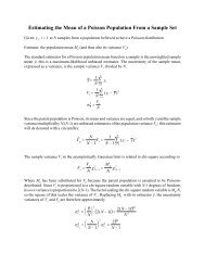
usage of PCA: Probability distribution for sample PCs
If (i) the n observations of in the sample are independent &
(ii)
is drawn from an underlying population that
follows a p-variate normal (Gaussian) distribution
with known covariance matrix
then
where
is the Wishart distribution
else
utilize a bootstrap approximation

usage of PCA: Probability distribution for sample PCs
If (i) follows a Wishart distribution &
(ii) the population eigenvalues
are all distinct
then
the following results hold as
• all the
are independent of all the
•are jointly normally distributed
(a tilde denotes a population quantity)

and
usage of PCA: Probability distribution for sample PCs
(a tilde denotes a population quantity)
•

usage of PCA: Inference about population PCs
If
then
follows a p-variate normal distribution
analytic expressions exist* for
MLE’s of , , and
confidence intervals for
hypothesis testing for
and
and
else
bootstrap and jackknife approximations exist
*see references, esp. Jolliffe

usage of PCA: Practical computation of PCs
In general it is useful to define standardized variables by
If the are each measured about their sample mean
then the covariance matrix of
will be equal to the correlation matrix of
and the PCs will be dimensionless

usage of PCA: Practical computation of PCs
Given a sample of n observations on a vector
(each measured about its sample mean)
of p variables
compute the covariance matrix
where
is the n x p matrix
whose i th row is the i th obsv.
Then compute the n x p matrix
whose i th row is the PC score
for the i th observation.

usage of PCA: Practical computation of PCs
Write
to decompose each observation into PCs

usage of PCA: Data compression
Because the k th PC retains the k th greatest fraction of the variation
we can approximate each observation
by truncating the sum at the first m < p PCs

usage of PCA: Data compression
Reduce the dimensionality of the data
from p to m < p by approximating
where
and
is the n x m portion of
is the p x m portion of

astronomical application: PCs for elliptical galaxies
Rotating to PC in B T – Σ space improves Faber-Jackson relation
as a distance indicator
Dressler, et al. 1987

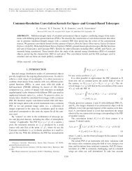
astronomical application: Eigenspectra (KL transform)
Connolly, et al. 1995

eferences
Connolly, and Szalay, et al., “Spectral Classification of Galaxies: An Orthogonal Approach”, AJ, 110, 1071-1082, 1995.
Dressler, et al., “Spectroscopy and Photometry of Elliptical Galaxies. I. A New Distance Estimator”, ApJ, 313, 42-58, 1987.
Efstathiou, G., and Fall, S.M., “Multivariate analysis of elliptical galaxies”, MNRAS, 206, 453-464, 1984.
Johnston, D.E., et al., “SDSS J0903+5028: A New Gravitational Lens”, AJ, 126, 2281-2290, 2003.
Jolliffe, Ian T., 2002, Principal Component Analysis (Springer-Verlag New York, Secaucus, NJ).
Lupton, R., 1993, Statistics In Theory and Practice (Princeton University Press, Princeton, NJ).
Murtagh, F., and Heck, A., Multivariate Data Analysis (D. Reidel Publishing Company, Dordrecht, Holland).
Yip, C.W., and Szalay, A.S., et al., “Distributions of Galaxy Spectral Types in the SDSS”, AJ, 128, 585-609, 2004.