Infrared astronomy: an introduction - School of Physics
Infrared astronomy: an introduction - School of Physics
Infrared astronomy: an introduction - School of Physics

Create successful ePaper yourself
Turn your PDF publications into a flip-book with our unique Google optimized e-Paper software.
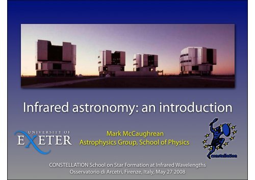
<strong>Infrared</strong> <strong>astronomy</strong>: <strong>an</strong> <strong>introduction</strong><br />
Mark McCaughre<strong>an</strong><br />
Astrophysics Group, <strong>School</strong> <strong>of</strong> <strong>Physics</strong><br />
CONSTELLATION <strong>School</strong> on Star Formation at <strong>Infrared</strong> Wavelengths<br />
Osservatorio di Arcetri, Firenze, Italy, May 27 2008
The original infrared observers<br />
Albino rattlesnake<br />
Mark Kostich
Western diamondback rattlesnake<br />
Aaron Krochmal, George Bakken / Indi<strong>an</strong>a State
Rattlesnake pit<br />
Wikipedia<br />
Western diamondback rattlesnake<br />
5-30µm thermal radiation impinges on<br />
15µm thick pit membr<strong>an</strong>e containing<br />
~2000 heat-sensitive nerve endings<br />
Temperature resolution > 0.001C<br />
Latency 50-150 msec<br />
Imaging via pinhole camera effect,<br />
enh<strong>an</strong>ced with neural processing<br />
Aaron Krochmal, George Bakken / Indi<strong>an</strong>a State
Rattlesnake nemesis<br />
California ground squirrel<br />
Gregg Elovich
Brave little buggers<br />
Ground squirrels versus a gopher snake<br />
US National Park Service
But clever too ...<br />
Ground squirrel versus gopher snake<br />
(no infrared sensory org<strong>an</strong>s)<br />
Ground squirrel versus rattlesnake<br />
(member <strong>of</strong> pit viper family)<br />
Thermal-infrared imaging<br />
Aaron Rundus, Donald Owings / UC Davis / New Scientist
More thermal infrared imaging
Hum<strong>an</strong> discovery <strong>of</strong> the infrared<br />
Herschel made discovery<br />
serendipitously in 1800<br />
Experiment to measure<br />
efficiency <strong>of</strong> filters<br />
Dispersed sunlight with prism<br />
Used thermometers: basic<br />
form <strong>of</strong> bolometer<br />
Found peak temperature<br />
beyond red end <strong>of</strong> visible<br />
spectrum<br />
Said due to “calorific rays”<br />
Soon after, Ritter similarly<br />
discovered the ultraviolet<br />
William Herschel
Actually, Herschel screwed up<br />
Peak <strong>of</strong> solar flux is at ~0.5 µm<br />
Why did Herschel measure peak at ~1 µm?<br />
Figures due to Tom Chester
Brief history <strong>of</strong> early infrared <strong>astronomy</strong><br />
1800: Herschel discovers infrared emission from Sun<br />
1856: Piazzi Smyth detects Moon from Tenerife<br />
1870: Earl <strong>of</strong> Rosse measures Moon’s temperature<br />
1878: L<strong>an</strong>gley invents infrared bolometer<br />
1915: Coblentz, Nicholson, Pettit, et al. measure<br />
Jupiter, Saturn, stars, nebulae, using thermopile<br />
1960: Johnson establishes first IR photometric system<br />
1968: Neugebauer, Leighton make first IR sky survey<br />
1974: Kuiper Airborne Observatory enters operation<br />
1983: IRAS makes first space IR survey<br />
1987: First common-user IR imaging systems
Some physics: black-body radiation<br />
Definition <strong>of</strong> “black”<br />
“Black” surface absorbs all light at all wavelengths incident upon it<br />
Definition <strong>of</strong> “blackbody radiation”<br />
To remain thermal equilibrium with surroundings, black surface<br />
must then emit just as much energy as it absorbs<br />
Spectrum <strong>of</strong> re-emitted radiation does not depend on spectrum<br />
<strong>of</strong> absorbed radiation<br />
Spectrum depends only on temperature <strong>of</strong> black surface<br />
Derivation <strong>of</strong> spectrum non-trivial<br />
Attempts by Rayleigh, Je<strong>an</strong>s, & Wien: ~ right at long λ, grows<br />
infinite at short λ; origin <strong>of</strong> so-called “UV catastrophe”<br />
Correct form determined by Max Pl<strong>an</strong>ck in 1900<br />
Required qu<strong>an</strong>tised energy E = hν: beginning <strong>of</strong> QM
Pl<strong>an</strong>ck’s Law for blackbody radiation<br />
I(ν, T) = 2hν3<br />
c 2 1<br />
e hν<br />
kT − 1<br />
I(λ, T) = 2hc2<br />
λ 5 1<br />
e hc<br />
λkT − 1<br />
Energy emitted<br />
per unit time<br />
per unit surface area<br />
per unit solid <strong>an</strong>gle<br />
per unit frequency<br />
J s -1 m -2 sr -1 Hz -1<br />
Note those are only equal in the following form:<br />
I(ν, T) dν = I(λ, T) dλ<br />
Convert between two forms using:<br />
Energy emitted<br />
per unit time<br />
per unit surface area<br />
per unit solid <strong>an</strong>gle<br />
per unit wavelength<br />
J s -1 m -2 sr -1 m -1<br />
c = νλ ⇒ ν = c λ ⇒ dν = − c λ 2 dλ
Pl<strong>an</strong>ck’s Law: linear blackbody curves<br />
4<br />
T=5500K<br />
Intensity (arbitrary linear units)<br />
3<br />
2<br />
1<br />
T=5000K<br />
T=4500K<br />
T=4000K<br />
T=3500K<br />
0<br />
0 500 1000 1500 2000<br />
Wavelength (nm)<br />
Adapted from Wikipedia
Pl<strong>an</strong>ck’s Law: logarithmic blackbody curves<br />
Intensity (arbitrary logarithmic units)<br />
10 13 T=10 000K<br />
Wien’s Displacement Law:<br />
Peak wavelength x Temperature is const<strong>an</strong>t<br />
10 11<br />
10 9<br />
10 7<br />
10 5<br />
10 3<br />
T=3000K<br />
T=1000K<br />
For λ in µm, T in K, const<strong>an</strong>t ª 3000<br />
e.g. for 3000K, peak at 1 µm;<br />
for 300K, peak at 10 µm<br />
T=300K<br />
10 1 0.1 1 10 100<br />
Wavelength (microns)
Key features <strong>of</strong> Pl<strong>an</strong>ck’s Law (I)<br />
Wien’s Displacement Law<br />
Peak wavelength x Temperature = const<strong>an</strong>t<br />
Peak λ (µm) x Temp (K) = 2897.7768 µm K<br />
Blackbody curves do not overlap<br />
Object at temperature T2 emits more photons (per unit<br />
everything) at all wavelengths th<strong>an</strong> object at T1, if T2 > T1<br />
Total power emitted given by Stef<strong>an</strong>-Boltzm<strong>an</strong>n Law<br />
Per unit area, but integrated over all wavelengths, all <strong>an</strong>gles<br />
P = σT 4 where σ = 2π5 k 4<br />
For object with emissivity ε<br />
<strong>an</strong>d total area A:<br />
P = σɛAT 4<br />
C<strong>an</strong> <strong>of</strong>ten make up for low T<br />
with very large A: import<strong>an</strong>t!<br />
15c 2 h 3<br />
Import<strong>an</strong>t note!<br />
Frequency equivalent:<br />
Peak ν (Hz) x Temp (K)<br />
= 5.879 x 10 10 Hz K<br />
But Peak ν ≠ (c/Peak λ)<br />
= 5.6704 × 10 −8 Js −1 m −2 K −4
Key features <strong>of</strong> Pl<strong>an</strong>ck’s Law (II)<br />
Long λ behaviour governed by “Rayleigh-Je<strong>an</strong>s tail”<br />
I(λ, T) = 2hc2<br />
λ 5 1<br />
e hc<br />
λkT − 1<br />
For large λ, hc/λkT
Low-temperature astronomical sources<br />
Bottom end <strong>of</strong> stellar initial mass function<br />
M, L dwarfs T eff typically 3000-1500K, peak ~1-2µm<br />
Coolest known T dwarfs ~800K, peak ~4µm<br />
More complicated in reality: molecular atmospheres<br />
Inner regions <strong>of</strong> circumstellar disks<br />
<strong>Infrared</strong> excess emission, CO b<strong>an</strong>dheads 2-2.5µm<br />
Terrestrial pl<strong>an</strong>et-forming regions in disks<br />
Liquid water requires ~300K, ~10µm<br />
Outer regions <strong>of</strong> disks<br />
Gas depletion due to gas gi<strong>an</strong>t formation ~100K, 30µm<br />
Molecular clouds, prestellar cores dust <strong>an</strong>d gas<br />
100-10K, 30-300µm: connection to sub-millimetre
Orion: the nearest major stellar nursery<br />
IRAS 12/60/100µm
The Orion Nebula star-forming region<br />
Optical: <strong>Infrared</strong>: Robberto McCaughre<strong>an</strong> / HST / VLT ACS/ ISAAC
<strong>Infrared</strong> penetrates dust extinction<br />
Cardelli, Clayton, & Mathis 1989
Dust extinction qu<strong>an</strong>tified<br />
Reduced effects <strong>of</strong> dust in near- <strong>an</strong>d mid-infrared:<br />
Worked example:<br />
Filter λ c A λ /A V<br />
V 0.55 1.000<br />
J 1.21 0.282<br />
H 1.65 0.175<br />
K 2.20 0.112<br />
L 3.45 0.058<br />
M 4.80 0.023<br />
N 10.0 0.052<br />
Take extinction <strong>of</strong> 25 magnitudes at V: dimming by 10 10<br />
In K-b<strong>an</strong>d, would be 2.8 magnitudes: dimming by 13<br />
In M-b<strong>an</strong>d, would be 0.6 magnitudes: dimming by 4
Reducing the effects <strong>of</strong> extinction<br />
Barnard 68<br />
Optical<br />
+ <strong>Infrared</strong> Alves et al. 2001, Nature
M16, The Eagle Nebula<br />
NOAO / Rector
Star formation in the “Pillars <strong>of</strong> Creation”?<br />
Optical: HST<br />
Hester & Scowen<br />
<strong>Infrared</strong>: VLT<br />
McCaughre<strong>an</strong> & Andersen
Line diagnostics <strong>an</strong>d astrochemistry<br />
Molecular absorption b<strong>an</strong>ds in stars<br />
TiO, VO, H 2 O, CH 4 , etc.<br />
Emission lines from ionised nebulae<br />
Hydrogen Paschen, Brackett, Pfund series<br />
Fe, O, He, Mg, Cr, Si, N, Ca, Ar, Ne, P, C, ...<br />
Emission/absorption lines in protostars<br />
Minerals: SiO, SiC, amorphous/crystalline<br />
Ices: CO, H 2 O, CO 2 , CH 4<br />
PAH features: complex C compounds<br />
Molecular lines<br />
Shocked/fluorescent H 2
Ices in <strong>an</strong>d around protostars
Evolution <strong>of</strong> circumstellar material<br />
ISO SWS spectra<br />
v<strong>an</strong> Dishoeck
Accretion, outflow, <strong>an</strong>d feedback<br />
HH212: VLT/ISAAC 6 hours integration time in the 2.12μm H 2 v=1-0 S(1) line (McCaughre<strong>an</strong> et al. 2002)
Proper motions over seven two years<br />
HH212: VLT/ISAAC HH212: VLT/ISAAC 2 hours Oct integration 2000 - VLT/HAWK-I time J<strong>an</strong> per 2008 epoch (McCaughre<strong>an</strong> et al., in et prep.) al., in prep.)
The evolution <strong>of</strong> the Universe
High-redshift <strong>astronomy</strong><br />
Redshift: λ obs = (1+z) λ em<br />
Classical galaxy diagnostics in mid-optical:<br />
Hα, Hβ, Ca H & K, 4000Å break, etc.<br />
Move to near-infrared at z=2-3<br />
Move to thermal-infrared at z=5-10<br />
Move to mid-infrared at z=20-30<br />
Lyα at 1216Å:<br />
Moves to near-infrared at z>7<br />
Cosmic microwave background:<br />
Blackbody radiation from ionised plasma at ~3000K<br />
Wien’s Law says peak should be at at ~1μm<br />
But epoch <strong>of</strong> recombination was at z~1000<br />
Should now be at ~3K, so peak at ~1000μm, i.e. 1 millimetre
Redshifted diagnostics<br />
NIR<br />
MIR
Redshifted emission from dist<strong>an</strong>t objects<br />
Hubble Ultradeep Field: NASA / ESA
Boosting sensitivity via gravitational lensing<br />
Abell 1689: HST+ACS (g, r, i, z)<br />
NASA / ESA / Benitez et al.
Recap<br />
<strong>Infrared</strong> <strong>astronomy</strong> driven by four factors:<br />
Access to low-temperature blackbodies<br />
Mitigation <strong>of</strong> dust extinction<br />
Emission <strong>an</strong>d absorption line diagnostics for astrochemistry<br />
Galaxies <strong>an</strong>d AGN at high redshift<br />
First three make the infrared vital for star <strong>an</strong>d pl<strong>an</strong>et<br />
formation studies<br />
But infrared <strong>astronomy</strong> is not that easy<br />
Absorption by terrestrial atmosphere<br />
Emission by terrestrial atmosphere<br />
Thermal background from telescope<br />
Unconventional detector technologies<br />
Photons “weaker” at longer wavelengths
Opening up the electromagnetic spectrum<br />
20th century saw entire EM spectrum<br />
from γ-rays to radio made available
Atmospheric tr<strong>an</strong>smission
<strong>Infrared</strong> tr<strong>an</strong>smission windows<br />
Léna, Lebrun, & Mignard
J, H, K, L windows<br />
J H K<br />
L<br />
Glass
M, N, Q windows<br />
M<br />
N<br />
Q<br />
Glass
Johnson optical-infrared filter system<br />
Filter λ (µm) Δλ (µm) Filter λ (µm) Δλ (µm)<br />
U 0.36 0.15 H 1.65 0.23<br />
B 0.44 0.22 K 2.2 0.34<br />
V 0.55 0.16 L’ 3.8 0.60<br />
R 0.64 0.23 M’ 4.7 0.22<br />
I 0.79 0.19 N 10 6.5<br />
J 1.26 0.16 Q 20 12<br />
There are m<strong>an</strong>y variations on this basic set, optimised for different sites, detectors, science<br />
Filter λ (µm) Δλ (µm) F λ (W m -2 µm -1 ) F ν (W m -2 Hz -1 ) J<strong>an</strong>sky<br />
U 0.36 0.15 4.19 x 10 -8 1.81 x 10 -23 1 810<br />
B 0.44 0.22 6.60 x 10 -8 4.26 x 10 -23 4 260<br />
V 0.55 0.16 3.51 x 10 -8 3.54 x 10 -23 3 540<br />
R 0.64 0.23 1.80 x 10 -8 2.94 x 10 -23 2 940<br />
I 0.79 0.19 9.76 x 10 -9 2.64 x 10 -23 2 640<br />
J 1.26 0.16 3.21 x 10 -9 1.67 x 10 -23 1 670<br />
H 1.65 0.23 1.08 x 10 -9 9.81 x 10 -24 981<br />
K 2.20 0.34 3.84 x 10 -10 6.20 x 10 -24 620
Sources <strong>of</strong> background flux<br />
Several components to background emission<br />
All strong function <strong>of</strong> wavelength<br />
Telescope:<br />
Thermal blackbody emission at ~270-280K<br />
Atmospheric:<br />
Thermal blackbody emission at ~220-230K<br />
Scattered moonlight<br />
Line emission (Lyα, O 2 , OI), OH airglow<br />
Celestial:<br />
Zodiacal dust (scattered sunlight <strong>an</strong>d thermal emission)<br />
Unresolved faint stars<br />
<strong>Infrared</strong> cirrus<br />
Cosmic microwave background
Zodiacal light<br />
Tony & Daphne Hallas
Gegenschein<br />
Yuri Beletsky / ESO
Scattering <strong>an</strong>d emission from zodiacal dust<br />
Léna, Lebrun, & Mignard
Gemini-N
Antarctic OH airglow movie (2002)<br />
Airglow movies
Near-infrared OH airglow<br />
Ennico / COHSI
<strong>Infrared</strong> cirrus<br />
IRAS
Cosmic microwave background<br />
Ait<strong>of</strong>f projection showing temperature fluctuations in CMB<br />
NASA / WMAP
Sky background spectrum<br />
Glass / Leinert / COBE
Import<strong>an</strong>ce <strong>of</strong> telescope thermal emission<br />
T eff<br />
= 280 K<br />
ε = 0.15<br />
Telescope<br />
Atmosphere<br />
Léna, Lebrun, & Mignard
Everest as seen from the ISS
Mauna Kea in the Pacific Oce<strong>an</strong><br />
Wainscoat
Cerro Par<strong>an</strong>al in the Chile<strong>an</strong> Atacama desert
Antarctica: the coldest continent on Earth<br />
South Pole<br />
Dome A<br />
Dome C
Concordia Station, Dome C, Antarctica<br />
IPEV IPEV / PNRA / PNRA / Dargaud / UNSW
Airborne infrared <strong>astronomy</strong>: SOFIA<br />
NASA / DLR
<strong>Infrared</strong> <strong>astronomy</strong> in space<br />
Get above the atmosphere<br />
Eliminate thermal/non-thermal sky emission: lower background<br />
Eliminate seeing: achieve diffraction-limited resolution<br />
Eliminate absorption: equal access to all wavelengths<br />
How to reduce telescope thermal background?<br />
Any object at ~1AU from Sun will have ~ same temperature as<br />
Earth, minus ~20K-worth <strong>of</strong> greenhouse effect<br />
HST actually actively heated to keep mirror at room temperature<br />
Solutions<br />
Move further away from Sun: temperature at 5AU ~ 120K<br />
Cool entire telescope/instrument package with cryogens<br />
Use sunshield to passively cool telescope
A brief history <strong>of</strong> IR space <strong>astronomy</strong><br />
Early days<br />
AFCRL/AFGL survey rocket flights<br />
The first orbiting space infrared survey<br />
IRAS<br />
The first orbiting space infrared observatory<br />
ISO<br />
Subsequent infrared missions<br />
IRTS, HST/NICMOS, MSX, Akari, Spitzer<br />
The future <strong>of</strong> space infrared <strong>astronomy</strong><br />
HST/WFC3, Herschel, WISE, JWST, (Darwin/TPF, SAFIR, FIRI, ...)<br />
(Excludes m<strong>an</strong>y other IR missions:<br />
COBE, WMAP, ODIN, SWAS, SL-2, WIRE, solar system ...)
IRAS: <strong>Infrared</strong> Astronomy Satellite (1983)<br />
NASA / NL / UK
IRAS (almost) all-sky survey<br />
Yellow-red horizontal strip is the galactic pl<strong>an</strong>e<br />
Blue S-shaped feature is the ecliptic<br />
NASA / NL / UK
IRTS: <strong>Infrared</strong> Telescope in Space (1995)<br />
JAXA
IRTS survey coverage <strong>an</strong>d results<br />
JAXA
ISO: <strong>Infrared</strong> Space Observatory (1995)<br />
ESA
M16, the Eagle Nebula with ISO<br />
ESA
MSX: Mid-Course Space Experiment (1996)<br />
US BMDO
Galactic centre with MSX<br />
US BMDO
HST NICMOS (1997)<br />
NASA / ESA
Orion Nebula & Trapezium Cluster<br />
Luhm<strong>an</strong> et al. / NASA / ESA
Spitzer Space Telescope (2003)<br />
Telescope<br />
Solar p<strong>an</strong>el<br />
shield<br />
Solar<br />
p<strong>an</strong>el<br />
Outer<br />
shell<br />
Spacecraft<br />
shield<br />
Spacecraft<br />
bus<br />
High gain<br />
<strong>an</strong>tenna<br />
Low gain<br />
<strong>an</strong>tennae<br />
Star trackers<br />
<strong>an</strong>d inertial<br />
reference units<br />
NASA
Herschel Space Observatory (2009)<br />
ESA
The role <strong>of</strong> infrared array detectors<br />
Number <strong>of</strong> pixels<br />
10 7<br />
10 5<br />
This infrared “Moore’s Law”<br />
(pixels double in 18 months)<br />
predicts > gigapixel<br />
cameras in ten years time<br />
10 9 2015<br />
256x256<br />
1024x1024<br />
512x512<br />
2048x2048<br />
4096x4096<br />
NICMOS<br />
Spitzer<br />
WFC3<br />
JWST<br />
128x128<br />
MSX<br />
10 3<br />
32x32<br />
62x58, 64x64<br />
ISO<br />
Space lags ground<br />
by ~ 9 years<br />
1985 1995<br />
2005<br />
Year<br />
After Al<strong>an</strong> H<strong>of</strong>fm<strong>an</strong>
Basic techniques for detecting IR photons<br />
Aim: convert incoming photons into electrical signals<br />
Photoconductors (0.3-30μm):<br />
Photons generate electron-hole pairs in semiconductors<br />
Electrons move to conduction b<strong>an</strong>d<br />
Electrons swept by electric field <strong>an</strong>d measured<br />
Bolometers (30-1000μm):<br />
Photons heat bulk material (semi- or superconductor)<br />
Temperature ch<strong>an</strong>ge induces ch<strong>an</strong>ge in electrical properties<br />
Heterodyne systems (100-1000μm):<br />
Mix incoming electromagnetic waves with local oscillator<br />
Detect amplitude <strong>of</strong> beat signal at much lower frequency<br />
Low noise electronics then used to amplify signal<br />
Coherent detection: preserves phase → interferometry
Energy b<strong>an</strong>d diagrams<br />
Insulator<br />
E g > 3.5eV<br />
Semiconductor<br />
0eV < E g < 3.5eV<br />
Conductor<br />
E g = 0eV<br />
1eV = 1.602 x 10 -19 J ≈ 1.24μm<br />
Rieke
Detector materials in the Periodic Table<br />
Typical semiconductors used in photoconductors include:<br />
Group IV: Ge, Si<br />
Group III-V: GaAs, InAs, InSb<br />
Group II-VI: CdS, CdTe<br />
Group IV-VI: PbS, PbSe, PbTe<br />
Rieke
Intrinsic semiconductor properties<br />
Material<br />
B<strong>an</strong>dgap<br />
(eV)<br />
Cut<strong>of</strong>f<br />
(μm)<br />
CdS 2.4 0.5<br />
CdSe 1.8 0.7<br />
GaAs 1.35 0.92<br />
Si 1.12 1.11<br />
Ge 0.67 1.85<br />
Hg x Cd 1-x Te (x=0.554) 0.5 2.5<br />
PbS 0.42 2.95<br />
InSb 0.23 5.4<br />
Hg x Cd 1-x Te (x=0.8) 0.1 12.4
Extrinsic semiconductor properties<br />
Material<br />
B<strong>an</strong>dgap<br />
(eV)<br />
Cut<strong>of</strong>f<br />
(μm)<br />
Si:In 0.16 7.9<br />
Si:Ga 0.072 17.2<br />
Si:As 0.054 23<br />
Si:Sb 0.043 29<br />
Si:As (BIB) 0.041 30<br />
Si:Sb (BIB) 0.031 40<br />
Ge:Ga 0.011 115<br />
Ge:Ga (stressed) 0.0062 >200
<strong>Infrared</strong> arrays<br />
Until early 1980s, only single element IR detectors<br />
Silicon microelectronics techniques widespread<br />
Spin<strong>of</strong>f was CCD detectors<br />
But IR semiconductors techniques not so well developed<br />
Answer: hybrid infrared arrays<br />
Use IR semiconductor for detection layer<br />
Use Si multiplexer for charge storage <strong>an</strong>d measurement<br />
Interface two mech<strong>an</strong>ically via metal interconnects<br />
IR material must backside illuminated<br />
Detector material must be thin<br />
Historically done via mech<strong>an</strong>ical polishing<br />
Now done via molecular beam epitaxy onto substrate
Schematic hybrid infrared array<br />
Detector array layer deposited on tr<strong>an</strong>sparent substrate e.g. sapphire<br />
Rieke
<strong>Infrared</strong> array evolution<br />
62x58 1987<br />
2048x2048 2001<br />
256x256 1991<br />
1024x1024 1996<br />
University <strong>of</strong> Rochester
WIRCam 4096x4096 HAWAII2RG mosaic<br />
as also used by HAWK-I on the VLT<br />
CFHT
Men <strong>an</strong>d their magnificent machines<br />
MJM I<strong>an</strong> McLe<strong>an</strong> <strong>an</strong>d his spectrograph <strong>an</strong>d IRCAM circa circa 1986 1982
HAWK-I on VLT UT4 Nasmyth platform<br />
ESO
Orion single-element mapping survey<br />
UKIRT / 2.2 microns / 5 & 3.5 arcsec beams / tens <strong>of</strong> sources<br />
Lonsdale, Becklin, Lee, & Stewart 1982
Single-element detector raster image<br />
AAT+IRPS / JHK b<strong>an</strong>ds / 2 arcsec pixels, 2 arcsec seeing / ~200 sources<br />
Allen, Bailey, & Hyl<strong>an</strong>d 1984, S&T
First IRCAM imaging mosaic <strong>of</strong> Orion<br />
UKIRT+IRCAM / K b<strong>an</strong>d / 0.6 arcsec pixels, 2 arcsec seeing / ~400 sources<br />
McCaughre<strong>an</strong> 1988, PhD thesis
Modern wide-field survey <strong>of</strong> Orion<br />
UKIRT+WFCAM / JKH 2 b<strong>an</strong>ds / 0.4 arcsec pixels, 1 arcsec seeing Davis, Varricat, Hirst, Casali et al. 2004
Contemporary deep survey <strong>of</strong> Orion<br />
VLT +ISAAC / J s HK s b<strong>an</strong>ds / 0.15 arcsec pixels, 0.4 arcsec seeing / ~1200 sources<br />
McCaughre<strong>an</strong> et al. 2002
Back to physics: Poisson distribution (I)<br />
One <strong>of</strong> m<strong>an</strong>y contributions by Poisson to mathematics<br />
Later work by Ladislaus Bortkiewicz, based on statistics <strong>of</strong><br />
number <strong>of</strong> soldiers kicked to death by horses <strong>an</strong>nually<br />
If me<strong>an</strong> expected number <strong>of</strong> discrete events (arrivals)<br />
in given time interval is N, then probability <strong>of</strong> there<br />
being exactly m occurrences is:<br />
f(m; N) = Nm e −N<br />
m!<br />
m must be non-negative integer (0, 1, 2, ...)<br />
N must be positive real number<br />
Derivation non-trivial: m<strong>an</strong>y available<br />
Siméon-Denis Poisson<br />
(Wikipedia)
Poisson distribution (II)<br />
N<br />
N<br />
N<br />
Probability<br />
m<br />
Adapted from Wikipedia
Poisson distribution (III)<br />
Key features:<br />
m c<strong>an</strong> only have integer values<br />
Lines joining values for illustration only<br />
m c<strong>an</strong>not be negative (obviously)<br />
Thus distribution is lop-sided for small N<br />
More symmetric for large N<br />
For our purposes, N is almost always large (>10)<br />
For large N, distribution is ~ normal with vari<strong>an</strong>ce = N<br />
f(x) =<br />
1<br />
σ √ 2π e −x2<br />
2σ 2 ⇒ f(m) ≈<br />
Normal distribution<br />
1<br />
√ e −m2<br />
2N<br />
2πN<br />
Poisson distribution for large N<br />
Vari<strong>an</strong>ce = σ 2 , thus st<strong>an</strong>dard deviation σ (or “noise”) √ <strong>of</strong><br />
a Poisson distribution with me<strong>an</strong> counts N = N<br />
N<br />
N<br />
N
Poisson distribution (IV)<br />
Import<strong>an</strong>t!<br />
Poisson statistics apply to the individual uncorrelated events<br />
actually registered in given time window<br />
Basic infrared array detector operation<br />
Incoming photon flux impinges on a pixel<br />
Some fraction converted into electrons<br />
Proceed to collect electrons for given integration time<br />
Cumulative charge creates voltage on pixel<br />
On read-out, voltage converted to counts by A/D converter<br />
Counts may be coadded over large number <strong>of</strong> integrations<br />
At which point do Poisson statistics get applied?<br />
Answer:<br />
Number <strong>of</strong> electrons collected per integration time
Application to signal-to-noise calculations<br />
1. Measure total flux through aperture centred on star:<br />
includes star, background, dark current, read-noise<br />
2. Measure average flux per pixel through larger <strong>an</strong>nulus:<br />
measures me<strong>an</strong> background, dark current; usually<br />
<strong>an</strong>nulus has larger area th<strong>an</strong> aperture, so error negligible<br />
3. Multiply average Histogram background <strong>of</strong> background / dark current flux: flux<br />
per pixel by area clearly <strong>of</strong> inner a normal aperture distribution<br />
4. Subtract background / dark current flux from value<br />
measured through star aperture; leaves star flux alone,<br />
but with Poisson noise <strong>of</strong> star, background, <strong>an</strong>d dark<br />
current, plus read-noise
Calculating astronomical S/N (I)<br />
Stellar flux: F photons s -1 m -2<br />
Stellar aperture area: M pixels<br />
πR 2 where R is radius <strong>of</strong> aperture in pixels<br />
Background flux: G photons s -1 m -2 pixel -1<br />
Assume well-measured over large <strong>an</strong>nulus; assume error-less<br />
Dark current: ID e - s -1 pixel -1<br />
Negligible for imaging; c<strong>an</strong> be import<strong>an</strong>t in spectroscopy<br />
Read-noise: RN e - pixel -1<br />
Typically measured in calibration experiment<br />
System throughput η<br />
Detector QE x (optical & atmospheric tr<strong>an</strong>smission)<br />
Integration time: t seconds<br />
Diameter <strong>of</strong> telescope: D m; Area A m 2
Calculating astronomical S/N (II)<br />
Measured stellar signal (in e - ) in stellar aperture:<br />
S = ηAFt<br />
Measured background signal (in e - ) in aperture:<br />
B = ηAGMt<br />
Measured dark current signal (in e - ) in aperture:<br />
D = I D Mt<br />
Total signal (in e - ) giving rise to Poisson noise:<br />
S + B + D = [ ηA(F + GM) + I D M ] t
Calculating astronomical S/N (III)<br />
Poisson noise due to star, background, dark current:<br />
Simply √ <strong>of</strong> total signal<br />
=<br />
√ [ηA(F + GM) + ID M ] t<br />
Read-noise over stellar aperture (e - RMS):<br />
Uncorrelated pixel-to-pixel: adds in quadrature over no. pixels<br />
= √ MR N<br />
Total noise added in quadrature:<br />
St<strong>an</strong>dard way <strong>of</strong> adding uncorrelated noise terms<br />
=<br />
√ [ηA(F + GM) + ID M ] t + MR N<br />
2
Calculating astronomical S/N (IV)<br />
Therefore, signal-to-noise:<br />
S<br />
N =<br />
ηAFt<br />
√ [ηA(F + GM) + ID M ] t + MR N<br />
2<br />
When F is large (bright star; “source noise limited” case):<br />
Background, dark current, <strong>an</strong>d read-noise terms negligible<br />
S<br />
N =<br />
ηAFt<br />
√<br />
ηAFt<br />
= √ ηAFt<br />
Thus doubling S/N requires:<br />
4 x integration time<br />
4 x collecting area
Read-noise limited case<br />
Full signal-to-noise:<br />
S<br />
N =<br />
ηAFt<br />
√ [ηA(F + GM) + ID M ] t + MR N<br />
2<br />
When F <strong>an</strong>d G small (very low background):<br />
Stellar & background shot noise, dark current terms negligible<br />
e.g. narrow-b<strong>an</strong>d imaging <strong>of</strong> faint sources or spectroscopy<br />
Here, doubling S/N requires:<br />
2 x integration time<br />
2 x collecting area<br />
2 x smaller RN<br />
S<br />
N =<br />
ηAFt<br />
√<br />
MRN
Background-limited case<br />
Full signal-to-noise:<br />
S<br />
N =<br />
When F is small but G large (bright background):<br />
Stellar shot noise, dark current, read-noise terms negligible<br />
S<br />
N =<br />
ηAFt<br />
√ [ηA(F + GM) + ID M ] t + MR N<br />
2<br />
ηAFt<br />
√<br />
ηAGMt<br />
= √ ηAt<br />
F<br />
√<br />
GM<br />
=<br />
Typical for broad-b<strong>an</strong>d imaging <strong>of</strong> faint sources<br />
Here, doubling S/N requires:<br />
4 x integration time<br />
4 x collecting area<br />
4 x lower background<br />
S √<br />
B
The case for big, cold telescopes<br />
For faint sources in the background-limit, we have:<br />
Thus time required to reach some given sensitivity<br />
<strong>an</strong>d<br />
S<br />
N = √ ηAt<br />
∝ 1 A ⇒ ∝ 1 D 2<br />
∝ GM<br />
F<br />
√<br />
GM<br />
⇒ t =<br />
( S<br />
N<br />
) 2<br />
1<br />
ηA<br />
GM<br />
F 2<br />
Thus maximising sensitivity <strong>of</strong> telescope requires:<br />
Maximising telescope diameter D<br />
Reducing background G as much as possible<br />
i.e. get above atmosphere <strong>an</strong>d make telescope cold<br />
Reducing number <strong>of</strong> pixels M covered by source<br />
Equivalent to reducing area covered by each pixel on sky
Reducing the area subtended by source<br />
Have assumed const<strong>an</strong>t image size (FWHM θ)<br />
~ true for seeing-limited observations<br />
What happens if θ is made smaller by factor <strong>of</strong> 2?<br />
C<strong>an</strong> make pixels smaller by factor 2<br />
Reduces area <strong>of</strong> pixel by factor 4<br />
Collect same amount <strong>of</strong> starlight from point source<br />
But only 1/4 <strong>of</strong> background<br />
In background-limited case<br />
S<br />
N = S √<br />
B<br />
⇒ S N ∝ 1 θ<br />
<strong>an</strong>d t ∝ θ 2<br />
Thus improving spatial resolution reduces integration time<br />
required for point sources
Impact <strong>of</strong> improved spatial resolution<br />
If diffraction-limited resolution c<strong>an</strong> be achieved:<br />
Using adaptive optics on ground or going into space<br />
Dependence <strong>of</strong> image size θ on telescope diameter D <strong>an</strong>d<br />
wavelength λ:<br />
θ (radi<strong>an</strong>s) = 1.22 λ (metres)<br />
D (metres)<br />
⇒<br />
θ (arcsec) = 0.25 λ (microns)<br />
D (metres)<br />
Thus<br />
θ ∝ 1 D ⇒ θ2 ∝ 1 D 2 ⇒ t ∝ 1 D 2<br />
Therefore, combined time required to reach given S/N:<br />
For diffraction-limited, background-limited point source<br />
t ∝ 1 D 2 × 1 D 2 ⇒ t ∝ 1 D 4<br />
Diffraction<br />
limited<br />
Background<br />
limited<br />
Thus big telescopes good,<br />
big cold telescopes better!
Europe<strong>an</strong> Extremely Large Telescope<br />
ESO
James Webb Space Telescope (2013)
An overview <strong>of</strong> the JWST<br />
6.5m deployable primary<br />
Diffraction-limited at 2µm<br />
Wavelength r<strong>an</strong>ge 0.6-28µm<br />
Sun-Earth L2 orbit<br />
4 instruments<br />
0.6-5µm wide field camera (NIRCam)<br />
1-5µm multiobject spectrometer (NIRSpec)<br />
Natural successor<br />
to HST & Spitzer<br />
5-28µm camera/spectrometer (MIRI)<br />
1-5µm fine guid<strong>an</strong>ce sensor / tunable filter imager (FGS/TFI)<br />
Passive cooling <strong>of</strong> telescope to
JWST: 7x area & 2.5x resolution <strong>of</strong> HST<br />
NASA / STScI
The extraordinary sensitivity <strong>of</strong> the JWST<br />
1000<br />
Broad-b<strong>an</strong>d (R~4) imaging<br />
Integration time 10 5 secs<br />
10 point source detection<br />
Flux (n<strong>an</strong>oJ<strong>an</strong>skys)<br />
100<br />
10<br />
Calibration: 2nJy or K Vega = 28.7<br />
which with JWST at R~4,<br />
yields 15 zeptowatts or<br />
1 photon every 5 seconds<br />
1<br />
1 3 10 30<br />
Wavelength (µm)
JWST star <strong>an</strong>d pl<strong>an</strong>et formation goals<br />
Trace deeply embedded phases <strong>of</strong> star formation<br />
Clouds ➞ cores ➞ protostars<br />
Investigate extreme ends <strong>of</strong> the Initial Mass Function<br />
Formation <strong>an</strong>d impact <strong>of</strong> massive stars<br />
Substellar IMF to pl<strong>an</strong>etary masses<br />
Examine the epoch <strong>of</strong> pl<strong>an</strong>et building<br />
Development <strong>of</strong> protopl<strong>an</strong>ets in young disks<br />
Follow astrochemical evolution<br />
Processing <strong>of</strong> gas, dust, & ice in cores, protostars, & disks<br />
Extend isolated paradigm to clustered, competitive<br />
star formation in a wide r<strong>an</strong>ge <strong>of</strong> environments<br />
Good match to goals <strong>of</strong> CONSTELLATION
Ari<strong>an</strong>e 5 ECA launch from Kourou to L2<br />
Long fairing<br />
(17m)<br />
Cryogenic<br />
upper stage<br />
H155<br />
core stage<br />
P230 solid<br />
propell<strong>an</strong>t<br />
booster<br />
Stowed configuration
Trajectory to L2
Summary<br />
Key questions to be <strong>an</strong>swered in star & pl<strong>an</strong>et formation<br />
What is the origin <strong>of</strong> the stellar mass distribution? Is it universal?<br />
What is the impact <strong>of</strong> feedback locally <strong>an</strong>d globally?<br />
How do disks turn into pl<strong>an</strong>etary systems?<br />
<strong>Infrared</strong> <strong>astronomy</strong> has a key role to play<br />
Greatly improved IR (& mm) sensitivity & spatial resolution needed<br />
Fortunately, the next decade will bring those resources<br />
VLTI<br />
E-ELT<br />
Antarctica<br />
ALMA<br />
JWST