Eternal inflation and its implications

MIT-CTP#3811 

hep-th/0702178 

Eternal inflation and its implications‡ 

arXiv:hep-th/0702178v1 22 Feb 2007 

Alan H. Guth 

Center for Theoretical Physics, Laboratory for Nuclear Science, and Department of 

Physics, Massachusetts Institute of Technology, Cambridge, MA 02139 

E-mail: guth@ctp.mit.edu 

Abstract. I summarize the arguments that strongly suggest that our universe is 

the product of inflation. The mechanisms that lead to eternal inflation in both 

new and chaotic models are described. Although the infinity of pocket universes 

produced by eternal inflation are unobservable, it is argued that eternal inflation has 

real consequences in terms of the way that predictions are extracted from theoretical 

models. The ambiguities in defining probabilities in eternally inflating spacetimes are 

reviewed, with emphasis on the youngness paradox that results from a synchronous 

gauge regularization technique. Although inflation is generically eternal into the future, 

it is not eternal into the past: it can be proven under reasonable assumptions that the 

inflating region must be incomplete in past directions, so some physics other than 

inflation is needed to describe the past boundary of the inflating region. 

‡ Talk presented at the 2nd International Conference on Quantum Theories and Renormalization 

Group in Gravity and Cosmology (IRGAC 2006), Barcelona, Spain, 11-15 July 2006, to be published 

in J. Phys. A.

Eternal inflation and its implications 2 

1. Introduction: the successes of inflation 

Since the proposal of the inflationary model some 25 years ago [1–4], inflation has 

been remarkably successful in explaining many important qualitative and quantitative 

properties of the universe. In this article I will summarize the key successes, and then 

discuss a number of issues associated with the eternal nature of inflation. In my opinion, 

the evidence that our universe is the result of some form of inflation is very solid. Since 

the term inflation encompasses a wide range of detailed theories, it is hard to imagine 

any reasonable alternative. The basic arguments are as follows: 

(i) The universe is big 

First of all, we know that the universe is incredibly large: the visible part of 

the universe contains about 10 90 particles. Since we have all grown up in a large 

universe, it is easy to take this fact for granted: of course the universe is big, it’s 

the whole universe! In “standard” FRW cosmology, without inflation, one simply 

postulates that about 10 90 or more particles were here from the start. However, in 

the context of present-day cosmology, many of us hope that even the creation of 

the universe can be described in scientific terms. Thus, we are led to at least think 

about a theory that might explain how the universe got to be so big. Whatever 

that theory is, it has to somehow explain the number of particles, 10 90 or more. 

However, it is hard to imagine such a number arising from a calculation in which 

the input consists only of geometrical quantities, quantities associated with simple 

dynamics, and factors of 2 or π. The easiest way by far to get a huge number, with 

only modest numbers as input, is for the calculation to involve an exponential. The 

exponential expansion of inflation reduces the problem of explaining 10 90 particles 

to the problem of explaining 60 or 70 e-foldings of inflation. In fact, it is easy to 

construct underlying particle theories that will give far more than 70 e-foldings of 

inflation. Inflationary cosmology therefore suggests that, even though the observed 

universe is incredibly large, it is only an infinitesimal fraction of the entire universe. 

(ii) The Hubble expansion 

The Hubble expansion is also easy to take for granted, since we have all known 

about it from our earliest readings in cosmology. In standard FRW cosmology, the 

Hubble expansion is part of the list of postulates that define the initial conditions. 

But inflation actually offers the possibility of explaining how the Hubble expansion 

began. The repulsive gravity associated with the false vacuum is just what Hubble 

ordered. It is exactly the kind of force needed to propel the universe into a pattern 

of motion in which any two particles are moving apart with a velocity proportional 

to their separation. 

(iii) Homogeneity and isotropy 

The degree of uniformity in the universe is startling. The intensity of the 

cosmic background radiation is the same in all directions, after it is corrected for 

the motion of the Earth, to the incredible precision of one part in 100,000. To get


some feeling for how high this precision is, we can imagine a marble that is spherical 

to one part in 100,000. The surface of the marble would have to be shaped to an 

accuracy of about 1,000 angstroms, a quarter of the wavelength of light. 

Although modern technology makes it possible to grind lenses to quarterwavelength 

accuracy, we would nonetheless be shocked if we unearthed a stone, 

produced by natural processes, that was round to an accuracy of 1,000 angstroms. 

If we try to imagine that such a stone were found, I am sure that no one would 

accept an explanation of its origin which simply proposed that the stone started 

out perfectly round. Similarly, I do not think it makes sense to consider any theory 

of cosmogenesis that cannot offer some explanation of how the universe became so 

incredibly isotropic. 

The cosmic background radiation was released about 300,000 years after the 

big bang, after the universe cooled enough so that the opaque plasma neutralized 

into a transparent gas. The cosmic background radiation photons have mostly 

been traveling on straight lines since then, so they provide an image of what the 

universe looked like at 300,000 years after the big bang. The observed uniformity of 

the radiation therefore implies that the observed universe had become uniform in 

temperature by that time. In standard FRW cosmology, a simple calculation shows 

that the uniformity could be established so quickly only if signals could propagate 

at 100 times the speed of light, a proposition clearly contradicting the known laws of 

physics. In inflationary cosmology, however, the uniformity is easily explained. The 

uniformity is created initially on microscopic scales, by normal thermal-equilibrium 

processes, and then inflation takes over and stretches the regions of uniformity to 

become large enough to encompass the observed universe. 

(iv) The flatness problem 

I find the flatness problem particularly impressive, because of the extraordinary 

numbers that it involves. The problem concerns the value of the ratio 

Ω tot ≡ ρ tot 

ρ c 

, (1) 

where ρ tot is the average total mass density of the universe and ρ c = 3H 2 /8πG is 

the critical density, the density that would make the universe spatially flat. (In the 

definition of “total mass density,” I am including the vacuum energy ρ vac = Λ/8πG 

associated with the cosmological constant Λ, if it is nonzero.) 

By combining data from the Wilkinson Microwave Anisotropy Probe 

(WMAP), the Sloan Digital Sky Survey (SDSS), and observations of type Ia 

supernovae, the authors of Ref. [5] deduced that the present value of Ω tot is equal 

to one within a few percent (Ω tot = 1.012 +0.018 

−0.022). Although this value is very close 

to one, the really stringent constraint comes from extrapolating Ω tot to early times, 

since Ω tot = 1 is an unstable equilibrium point of the standard model evolution. 

Thus, if Ω tot was ever exactly equal to one, it would remain exactly one forever. 

However, if Ω tot differed slightly from one in the early universe, that difference— 

whether positive or negative—would be amplified with time. In particular, it can


be shown that Ω tot − 1 grows as 

⎧ 

⎨t 

(during the radiation-dominated era) 

Ω tot − 1 ∝ 

⎩t 2/3 (during the matter-dominated era) . 

Dicke and Peebles [6] pointed out that at t = 1 second, for example, when the 

processes of big bang nucleosynthesis were just beginning, Ω tot must have equaled 

one to an accuracy of one part in 10 15 . Classical cosmology provides no explanation 

for this fact—it is simply assumed as part of the initial conditions. In the context 

of modern particle theory, where we try to push things all the way back to the 

Planck time, 10 −43 s, the problem becomes even more extreme. If one specifies the 

value of Ω tot at the Planck time, it has to equal one to 59 decimal places in order 

to be in the allowed range today. 

While this extraordinary flatness of the early universe has no explanation in 

classical FRW cosmology, it is a natural prediction for inflationary cosmology. 

During the inflationary period, instead of Ω tot being driven away from one as 

described by Eq. (2), Ω tot is driven towards one, with exponential swiftness: 

Ω tot − 1 ∝ e −2H inft , (3) 

where H inf is the Hubble parameter during inflation. Thus, as long as there is a 

long enough period of inflation, Ω tot can start at almost any value, and it will be 

driven to unity by the exponential expansion. 

(v) Absence of magnetic monopoles 

All grand unified theories predict that there should be, in the spectrum of 

possible particles, extremely massive particles carrying a net magnetic charge. By 

combining grand unified theories with classical cosmology without inflation, Preskill 

[7] found that magnetic monopoles would be produced so copiously that they would 

outweigh everything else in the universe by a factor of about 10 12 . A mass density 

this large would cause the inferred age of the universe to drop to about 30,000 

years! Inflation is certainly the simplest known mechanism to eliminate monopoles 

from the visible universe, even though they are still in the spectrum of possible 

particles. The monopoles are eliminated simply by arranging the parameters so 

that inflation takes place after (or during) monopole production, so the monopole 

density is diluted to a completely negligible level. 

(vi) Anisotropy of the cosmic background radiation 

The process of inflation smooths the universe essentially completely, but 

density fluctuations are generated as inflation ends by the quantum fluctuations 

of the inflaton field [8, 9]. Generically these are adiabatic Gaussian fluctuations 

with a nearly scale-invariant spectrum. 

Until recently, astronomers were aware of several cosmological models that 

were consistent with the known data: an open universe, with Ω ∼ = 0.3; an 

inflationary universe with considerable dark energy (Λ); an inflationary universe 

without Λ; and a universe in which the primordial perturbations arose from 

(2)


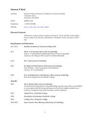
Figure 1. Comparison of the latest observational measurements of the temperature 

fluctuations in the CMB with several theoretical models, as described in the text. The 

temperature pattern on the sky is expanded in multipoles (i.e., spherical harmonics), 

and the intensity is plotted as a function of the multipole number l. Roughly speaking, 

each multipole l corresponds to ripples with an angular wavelength of 360 ◦ /l. 

topological defects such as cosmic strings. Each of these models leads to a distinctive 

pattern of resonant oscillations in the early universe, which can be probed today 

through its imprint on the CMB. As can be seen in Fig. 1 [20], three of the models 

are now definitively ruled out. The full class of inflationary models can make a 

variety of predictions, but the predictions of the simplest inflationary models with 

large Λ, shown on the graph, fit the data beautifully. 

2. Eternal Inflation: Mechanisms 

The remainder of this article will discuss eternal inflation—the questions that it can 

answer, and the questions that it raises. In this section I discuss the mechanisms that 

make eternal inflation possible, leaving the other issues for the following sections. I will 

discuss eternal inflation first in the context of new inflation, and then in the context of 

chaotic inflation, where it is more subtle. 

2.1. Eternal New Inflation 

The eternal nature of new inflation was first discovered by Steinhardt [24], and later 

that year Vilenkin [25] showed that new inflationary models are generically eternal.


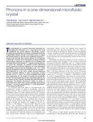
Figure 2. Evolution of the inflaton field during new inflation. 

Figure 3. A schematic illustration of eternal inflation. 

Although the false vacuum is a metastable state, the decay of the false vacuum is an 

exponential process, very much like the decay of any radioactive or unstable substance. 

The probability of finding the inflaton field at the top of the plateau in its potential 

energy diagram, Fig. 2, does not fall sharply to zero, but instead trails off exponentially 

with time [26]. However, unlike a normal radioactive substance, the false vacuum 

exponentially expands at the same time that it decays. In fact, in any successful 

inflationary model the rate of exponential expansion is always much faster than the 

rate of exponential decay. Therefore, even though the false vacuum is decaying, it 

never disappears, and in fact the total volume of the false vacuum, once inflation starts, 

continues to grow exponentially with time, ad infinitum. 

Fig. 3 shows a schematic diagram of an eternally inflating universe. The top bar 

indicates a region of false vacuum. The evolution of this region is shown by the successive 

bars moving downward, except that the expansion could not be shown while still fitting 

all the bars on the page. So the region is shown as having a fixed size in comoving 

coordinates, while the scale factor, which is not shown, increases from each bar to the 

next. As a concrete example, suppose that the scale factor for each bar is three times 

larger than for the previous bar. If we follow the region of false vacuum as it evolves from 

the situation shown in the top bar to the situation shown in the second bar, in about one


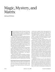
Figure 4. Evolution of the inflaton field during eternal chaotic inflation. 

third of the region the scalar field rolls down the hill of the potential energy diagram, 

precipitating a local big bang that will evolve into something that will eventually appear 

to its inhabitants as a universe. This local big bang region is shown in gray and labelled 

“Universe.” Meanwhile, however, the space has expanded so much that each of the two 

remaining regions of false vacuum is the same size as the starting region. Thus, if we 

follow the region for another time interval of the same duration, each of these regions of 

false vacuum will break up, with about one third of each evolving into a local universe, 

as shown on the third bar from the top. Now there are four remaining regions of false 

vacuum, and again each is as large as the starting region. This process will repeat itself 

literally forever, producing a kind of a fractal structure to the universe, resulting in an 

infinite number of the local universes shown in gray. There is no standard name for 

these local universes, but they are often called bubble universes. I prefer, however, to 

call them pocket universes, to avoid the suggestion that they are round. While bubbles 

formed in first-order phase transitions are round [27], the local universes formed in 

eternal new inflation are generally very irregular, as can be seen for example in the 

two-dimensional simulation by Vanchurin, Vilenkin, and Winitzki in Fig. 2 of Ref. [28]. 

The diagram in Fig. 3 is of course an idealization. The real universe is three 

dimensional, while the diagram illustrates a schematic one-dimensional universe. It is 

also important that the decay of the false vacuum is really a random process, while 

the diagram was constructed to show a very systematic decay, because it is easier to 

draw and to think about. When these inaccuracies are corrected, we are still left with 

a scenario in which inflation leads asymptotically to a fractal structure [29] in which 

the universe as a whole is populated by pocket universes on arbitrarily small comoving 

scales. Of course this fractal structure is entirely on distance scales much too large to 

be observed, so we cannot expect astronomers to see it. Nonetheless, one does have 

to think about the fractal structure if one wants to understand the very large scale 

structure of the spacetime produced by inflation. 

Most important of all is the simple statement that once inflation happens, it 

produces not just one universe, but an infinite number of universes.


2.2. Eternal Chaotic Inflation: 

The eternal nature of new inflation depends crucially on the scalar field lingering at the 

top of the plateau of Fig. 2. Since the potential function for chaotic inflation, Fig. 4, does 

not have a plateau, it is not obvious how eternal inflation can happen in this context. 

Nonetheless, Andrei Linde [30] showed in 1986 that chaotic inflation can also be eternal. 

In this case inflation occurs as the scalar field rolls down a hill of the potential 

energy diagram, as in Fig. 4, starting high on the hill. As the field rolls down the hill, 

quantum fluctuations will be superimposed on top of the classical motion. The best 

way to think about this is to ask what happens during one time interval of duration 

∆t = H −1 (one Hubble time), in a region of one Hubble volume H −3 . Suppose that 

φ 0 is the average value of φ in this region, at the start of the time interval. By the 

definition of a Hubble time, we know how much expansion is going to occur during the 

time interval: exactly a factor of e. (This is the only exact number in today’s talk, so I 

wanted to emphasize the point.) That means the volume will expand by a factor of e 3 . 

One of the deep truths that one learns by working on inflation is that e 3 is about equal 

to 20, so the volume will expand by a factor of 20. Since correlations typically extend 

over about a Hubble length, by the end of one Hubble time, the initial Hubble-sized 

region grows and breaks up into 20 independent Hubble-sized regions. 

As the scalar field is classically rolling down the hill, the change in the field ∆φ 

during the time interval ∆t is going to be modified by quantum fluctuations ∆φ qu , which 

can drive the field upward or downward relative to the classical trajectory. For any one 

of the 20 regions at the end of the time interval, we can describe the change in φ during 

the interval by 

∆φ = ∆φ cl + ∆φ qu , (4) 

where ∆φ cl is the classical value of ∆φ. In lowest order perturbation theory the 

fluctuations are calculated using free quantum field, which implies that ∆φ qu , the 

quantum fluctuation averaged over one of the 20 Hubble volumes at the end, will have 

a Gaussian probability distribution, with a width of order H/2π [13, 31–33]. There is 

then always some probability that the sum of the two terms on the right-hand side will 

be positive — that the scalar field will fluctuate up and not down. As long as that 

probability is bigger than 1 in 20, then the number of inflating regions with φ ≥ φ 0 will 

be larger at the end of the time interval ∆t than it was at the beginning. This process 

will then go on forever, so inflation will never end. 

Thus, the criterion for eternal inflation is that the probability for the scalar field 

to go up must be bigger than 1/e 3 ≈ 1/20. For a Gaussian probability distribution, 

this condition will be met provided that the standard deviation for ∆φ qu is bigger than 

0.61|∆φ cl |. Using ∆φ cl ≈ ˙φ cl H −1 , the criterion becomes 

∆φ qu ≈ H 2π > 0.61 | ˙φ cl | H −1 ⇐⇒ H2 

| ˙φ cl | 

> 3.8 . (5) 

We have not discussed the calculation of density perturbations in detail, but the


condition (5) for eternal inflation is equivalent to the condition that δρ/ρ on ultra-long 

length scales is bigger than a number of order unity. 

The probability that ∆φ is positive tends to increase as one considers larger and 

larger values of φ, so sooner or later one reaches the point at which inflation becomes 

eternal. If one takes, for example, a scalar field with a potential 

V (φ) = 1 4 λφ4 , (6) 

then the de Sitter space equation of motion in flat Robertson-Walker coordinates takes 

the form 

¨φ + 3H ˙φ = −λφ 3 , (7) 

where spatial derivatives have been neglected. In the “slow-roll” approximation one also 

neglects the ¨φ term, so ˙φ ≈ −λφ 3 /(3H), where the Hubble constant H is related to the 

energy density by 

H 2 = 8π 3 Gρ = 2π 3 

λφ 4 

M 2 p 

. (8) 

Putting these relations together, one finds that the criterion for eternal inflation, Eq. (5), 

becomes 

φ > 0.75 λ −1/6 M p . (9) 

Since λ must be taken very small, on the order of 10 −12 , for the density perturbations 

to have the right magnitude, this value for the field is generally well above the Planck 

scale. The corresponding energy density, however, is given by 

V (φ) = 1 4 λφ4 = .079λ 1/3 M 4 p , (10) 

which is actually far below the Planck scale. 

So for these reasons we think inflation is almost always eternal. I think the 

inevitability of eternal inflation in the context of new inflation is really unassailable 

— I do not see how it could possibly be avoided, assuming that the rolling of the scalar 

field off the top of the hill is slow enough to allow inflation to be successful. The 

argument in the case of chaotic inflation is less rigorous, but I still feel confident that it 

is essentially correct. For eternal inflation to set in, all one needs is that the probability 

for the field to increase in a given Hubble-sized volume during a Hubble time interval 

is larger than 1/20. 

Thus, once inflation happens, it produces not just one universe, but an infinite 

number of universes. 

3. Implications for the Landscape of String Theory 

Until recently, the idea of eternal inflation was viewed by most physicists as an oddity, 

of interest only to a small subset of cosmologists who were afraid to deal with concepts 

that make real contact with observation. The role of eternal inflation in scientific


thinking, however, was greatly boosted by the realization that string theory has no 

preferred vacuum, but instead has perhaps 10 1000 [34, 35] metastable vacuum-like states. 

Eternal inflation then has potentially a direct impact on fundamental physics, since it 

can provide a mechanism to populate the landscape of string vacua. While all of these 

vacua are described by the same fundamental string theory, the apparent laws of physics 

at low energies could differ dramatically from one vacuum to another. In particular, the 

value of the cosmological constant (e.g., the vacuum energy density) would be expected 

to have different values for different vacua. 

The combination of the string landscape with eternal inflation has in turn led to 

a markedly increased interest in anthropic reasoning, since we now have a respectable 

set of theoretical ideas that provide a setting for such reasoning. To many physicists, 

the new setting for anthropic reasoning is a welcome opportunity: in the multiverse, 

life will evolve only in very rare regions where the local laws of physics just happen to 

have the properties needed for life, giving a simple explanation for why the observed 

universe appears to have just the right properties for the evolution of life. The incredibly 

small value of the cosmological constant is a telling example of a feature that seems to 

be needed for life, but for which an explanation from fundamental physics is painfully 

lacking. Anthropic reasoning can give the illusion of intelligent design [36], without the 

need for any intelligent intervention. 

On the other hand, many other physicists have an abhorrence of anthropic 

reasoning. To this group, anthropic reasoning means the end of the hope that precise and 

unique predictions can be made on the basis of logical deduction [37]. Since this hope 

should not be given up lightly, many physicists are still trying to find some mechanism 

to pick out a unique vacuum from string theory. So far there is no discernable progress. 

It seems sensible, to me, to consider anthropic reasoning to be the explanation of 

last resort. That is, in the absence of any detailed understanding of the multiverse, 

life, or the evolution of either, anthropic arguments become plausible only when we 

cannot find any other explanation. That said, I find it difficult to know whether the 

cosmological constant problem is severe enough to justify the explanation of last resort. 

Inflation can conceivably help in the search for a nonanthropic explanation of 

vacuum selection, since it offers the possibility that only a small minority of vacua are 

populated. Inflation is, after all, a complicated mechanism that involves exponentially 

large factors in its basic description, so it possible that it populates some states 

overwhelming more than others. In particular, one might expect that those states that 

lead to the fastest exponential expansion rates would be favored. Then these fastest 

expanding states — and their decay products — could dominate the multiverse. 

But so far, unfortunately, this is only wishful thinking. As I will discuss in the 

next section, we do not even know how to define probabilities in eternally inflating 

multiverses. Furthermore, it does not seem likely that any principle that favors a rapid 

rate of exponential inflation will favor a vacuum of the type that we live in. The 

key problem, as one might expect, is the value of the cosmological constant. The 

cosmological constant Λ in our universe is extremely small, i.e., Λ < ∼ 10 −120 in Planck


units. If inflation singles out the state with the fastest exponential expansion rate, the 

energy density of that state would be expected to be of order Planck scale or larger. To 

explain why our vacuum has such a small energy density, we would need to find some 

reason why this very high energy density state should decay preferentially to a state 

with an exceptionally small energy density [38]. 

There has been some effort to find relaxation methods that might pick out the 

vacuum [39], and perhaps this is the best hope for a nonanthropic explanation of the 

cosmological constant. So far, however, the landscape of nonanthropic solutions to this 

problem seems bleak. 

4. Difficulties in Calculating Probabilities 

In an eternally inflating universe, anything that can happen will happen; in fact, it will 

happen an infinite number of times. Thus, the question of what is possible becomes 

trivial—anything is possible, unless it violates some absolute conservation law. To 

extract predictions from the theory, we must therefore learn to distinguish the probable 

from the improbable. 

However, as soon as one attempts to define probabilities in an eternally inflating 

spacetime, one discovers ambiguities. The problem is that the sample space is infinite, in 

that an eternally inflating universe produces an infinite number of pocket universes. The 

fraction of universes with any particular property is therefore equal to infinity divided 

by infinity—a meaningless ratio. To obtain a well-defined answer, one needs to invoke 

some method of regularization. 

To understand the nature of the problem, it is useful to think about the integers 

as a model system with an infinite number of entities. We can ask, for example, what 

fraction of the integers are odd. Most people would presumably say that the answer is 

1/2, since the integers alternate between odd and even. That is, if the string of integers 

is truncated after the Nth, then the fraction of odd integers in the string is exactly 1/2 

if N is even, and is (N + 1)/2N if N is odd. In any case, the fraction approaches 1/2 

as N approaches infinity. 

However, the ambiguity of the answer can be seen if one imagines other orderings 

for the integers. One could, if one wished, order the integers as 

1, 3, 2, 5, 7, 4, 9, 11, 6 , . . ., (11) 

always writing two odd integers followed by one even integer. This series includes each 

integer exactly once, just like the usual sequence (1, 2, 3, 4, . . .). The integers are just 

arranged in an unusual order. However, if we truncate the sequence shown in Eq. (11) 

after the Nth entry, and then take the limit N → ∞, we would conclude that 2/3 of 

the integers are odd. Thus, we find that the definition of probability on an infinite set 

requires some method of truncation, and that the answer can depend nontrivially on 

the method that is used. 

In the case of eternally inflating spacetimes, the natural choice of truncation might 

be to order the pocket universes in the sequence in which they form. However, we


must remember that each pocket universe fills its own future light cone, so no pocket 

universe forms in the future light cone of another. Any two pocket universes are spacelike 

separated from each other, so some observers will see one as forming first, while other 

observers will see the opposite. One can arbitrarily choose equal-time surfaces that 

foliate the spacetime, and then truncate at some value of t, but this recipe is not unique. 

In practice, different ways of choosing equal-time surfaces give different results. 

5. The Youngness Paradox 

If one chooses a truncation in the most naive way, one is led to a set of very peculiar 

results which I call the youngness paradox. 

Specifically, suppose that one constructs a Robertson-Walker coordinate system 

while the model universe is still in the false vacuum (de Sitter) phase, before any pocket 

universes have formed. One can then propagate this coordinate system forward with a 

synchronous gauge condition,§ and one can define probabilities by truncating at a fixed 

value t f of the synchronous time coordinate t. That is, the probability of any particular 

property can be taken to be proportional to the volume on the t = t f hypersurface which 

has that property. This method of defining probabilities was studied in detail by Linde, 

Linde, and Mezhlumian, in a paper with the memorable title “Do we live in the center 

of the world?” [40]. I will refer to probabilities defined in this way as synchronous gauge 

probabilities. 

The youngness paradox is caused by the fact that the volume of false vacuum is 

growing exponentially with time with an extraordinary time constant, in the vicinity of 

10 −37 s. Since the rate at which pocket universes form is proportional to the volume of 

false vacuum, this rate is increasing exponentially with the same time constant. That 

means that in each second the number of pocket universes that exist is multiplied by a 

factor of exp {10 37 }. At any given time, therefore, almost all of the pocket universes that 

exist are universes that formed very very recently, within the last several time constants. 

The population of pocket universes is therefore an incredibly youth-dominated society, 

in which the mature universes are vastly outnumbered by universes that have just barely 

begun to evolve. Although the mature universes have a larger volume, this multiplicative 

factor is of little importance, since in synchronous coordinates the volume no longer 

grows exponentially once the pocket universe forms. 

Probability calculations in this youth-dominated ensemble lead to peculiar results, 

as discussed in Ref. [40]. These authors considered the expected behavior of the mass 

density in our vicinity, concluding that we should find ourselves very near the center 

of a spherical low-density region. Here I would like to discuss a less physical but 

simpler question, just to illustrate the paradoxes associated with synchronous gauge 

probabilities. Specifically, I will consider the question: “Are there any other civilizations 

§ By a synchronous gauge condition, I mean that each equal-time hypersurface is obtained by 

propagating every point on the previous hypersurface by a fixed infinitesimal time interval ∆t in the 

direction normal to the hypersurface.


in the visible universe that are more advanced than ours?”. Intuitively I would not 

expect inflation to make any predictions about this question, but I will argue that the 

synchronous gauge probability distribution strongly implies that there is no civilization 

in the visible universe more advanced than us. 

Suppose that we have reached some level of advancement, and suppose that t min 

represents the minimum amount of time needed for a civilization as advanced as we are 

to evolve, starting from the moment of the decay of the false vacuum—the start of the 

big bang. The reader might object on the grounds that there are many possible measures 

of advancement, but I would respond by inviting the reader to pick any measure she 

chooses; the argument that I am about to give should apply to all of them. The reader 

might alternatively claim that there is no sharp minimum t min , but instead we should 

describe the problem in terms of a function which gives the probability that, for any 

given pocket universe, a civilization as advanced as we are would develop by time t. I 

believe, however, that the introduction of such a probability distribution would merely 

complicate the argument, without changing the result. So, for simplicity of discussion, 

I will assume that there is some sharply defined minimum time t min required for a 

civilization as advanced as ours to develop. 

Since we exist, our pocket universe must have an age t 0 satisfying 

t 0 ≥ t min . (12) 

Suppose, however, that there is some civilization in our pocket universe that is more 

advanced than we are, let us say by 1 second. In that case Eq. (12) is not sufficient, but 

instead the age of our pocket universe would have to satisfy 

t 0 ≥ t min + 1 second . (13) 

However, in the synchronous gauge probability distribution, universes that satisfy 

Eq. (13) are outnumbered by universes that satisfy Eq. (12) by a factor of approximately 

exp {10 37 }. Thus, if we know only that we are living in a pocket universe that satisfies 

Eq. (12), it is extremely improbable that it also satisfies Eq. (13). We would conclude, 

therefore, that it is extraordinarily improbable that there is a civilization in our pocket 

universe that is at least 1 second more advanced than we are. 

Perhaps this argument explains why SETI has not found any signals from alien 

civilizations, but I find it more plausible that it is merely a symptom that the 

synchronous gauge probability distribution is not the right one. 

Although the problem of defining probabilities in eternally inflating universe has 

not been solved, a great deal of progress has been made in exploring options and 

understanding their properties. For many years Vilenkin and his collaborators [28, 41] 

were almost the only cosmologists working on this issue, but now the field is growing 

rapidly [42].


6. Does Inflation Need a Beginning? 

If the universe can be eternal into the future, is it possible that it is also eternal into 

the past? Here I will describe a recent theorem [43] which shows, under plausible 

assumptions, that the answer to this question is no.‖ 

The theorem is based on the well-known fact that the momentum of an object 

traveling on a geodesic through an expanding universe is redshifted, just as the 

momentum of a photon is redshifted. Suppose, therefore, we consider a timelike or null 

geodesic extended backwards, into the past. In an expanding universe such a geodesic 

will be blueshifted. The theorem shows that under some circumstances the blueshift 

reaches infinite rapidity (i.e., the speed of light) in a finite amount of proper time (or 

affine parameter) along the trajectory, showing that such a trajectory is (geodesically) 

incomplete. 

To describe the theorem in detail, we need to quantify what we mean by an 

expanding universe. We imagine an observer whom we follow backwards in time along 

a timelike or null geodesic. The goal is to define a local Hubble parameter along this 

geodesic, which must be well-defined even if the spacetime is neither homogeneous nor 

isotropic. Call the velocity of the geodesic observer v µ (τ), where τ is the proper time 

in the case of a timelike observer, or an affine parameter in the case of a null observer. 

(Although we are imagining that we are following the trajectory backwards in time, 

τ is defined to increase in the future timelike direction, as usual.) To define H, we 

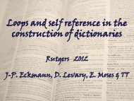
must imagine that the vicinity of the observer is filled with “comoving test particles,” 

so that there is a test particle velocity u µ (τ) assigned to each point τ along the geodesic 

trajectory, as shown in Fig. 5. These particles need not be real — all that will be 

necessary is that the worldlines can be defined, and that each worldline should have 

zero proper acceleration at the instant it intercepts the geodesic observer. 

To define the Hubble parameter that the observer measures at time τ, the observer 

focuses on two particles, one that he passes at time τ, and one at τ + ∆τ, where in the 

end he takes the limit ∆τ → 0. The Hubble parameter is defined by 

H ≡ ∆v radial 

, (14) 

∆r 

where ∆v radial is the radial component of the relative velocity between the two particles, 

and ∆r is their distance, where both quantities are computed in the rest frame of one of 

the test particles, not in the rest frame of the observer. Note that this definition reduces 

to the usual one if it is applied to a homogeneous isotropic universe. 

The relative velocity between the observer and the test particles can be measured 

by the invariant dot product, 

γ ≡ u µ v µ , (15) 

‖ There were also earlier theorems about this issue by Borde and Vilenkin (1994, 1996) [44, 45], and 

Borde [46] (1994), but these theorems relied on the weak energy condition, which for a perfect fluid 

is equivalent to the condition ρ + p ≥ 0. This condition holds classically for forms of matter that 

are known or commonly discussed as theoretical proposals. It can, however, be violated by quantum 

fluctuations [47], and so the applicability of these theorems is questionable.


Figure 5. An observer measures the velocity of passing test particles to infer the 

Hubble parameter. 

which for the case of a timelike observer is equal to the usual special relativity Lorentz 

factor 

1 

γ = √ . (16) 

1 − vrel 

2 

If H is positive we would expect γ to decrease with τ, since we expect the observer’s 

momentum relative to the test particles to redshift. It turns out, however, that the 

relationship between H and changes in γ can be made precise. If one defines 

⎧ 

⎨ 1/γ for null observers 

F(γ) ≡ 

(17) 

⎩ arctanh(1/γ) for timelike observers , 

then 

H = dF(γ) . (18) 

dτ 

I like to call F(γ) the “slowness” of the geodesic observer, because it increases as 

the observer slows down, relative to the test particles. The slowness decreases as we 

follow the geodesic backwards in time, but it is positive definite, and therefore cannot 

decrease below zero. F(γ) = 0 corresponds to γ = ∞, or a relative velocity equal to 

that of light. This bound allows us to place a rigorous limit on the integral of Eq. (18). 

For timelike geodesics, 

∫ ( ) 

τf 

1 

(√ ) 

H dτ ≤ arctanh = arctanh 1 − vrel 

2 , (19) 

γ f 

where γ f is the value of γ at the final time τ = τ f . For null observers, if we normalize 

the affine parameter τ by dτ/dt = 1 at the final time τ f , then 

∫ τf 

H dτ ≤ 1 . (20) 

Thus, if we assume an averaged expansion condition, i.e., that the average value of the 

Hubble parameter H av along the geodesic is positive, then the proper length (or affine 

length for null trajectories) of the backwards-going geodesic is bounded. Thus the region 

for which H av > 0 is past-incomplete.


It is difficult to apply this theorem to general inflationary models, since there is no 

accepted definition of what exactly defines this class. However, in standard eternally 

inflating models, the future of any point in the inflating region can be described by a 

stochastic model [48] for inflaton evolution, valid until the end of inflation. Except for 

extremely rare large quantum fluctuations, H > ∼ 

√ 

(8π/3)Gρf , where ρ f is the energy 

density of the false vacuum driving the inflation. The past for an arbitrary model is less 

certain, but we consider eternal models for which the past is like the future. In that 

case H would be positive almost everywhere in the past inflating region. If, however, 

H av > 0 when averaged over a past-directed geodesic, our theorem implies that the 

geodesic is incomplete. 

There is of course no conclusion that an eternally inflating model must have a 

unique beginning, and no conclusion that there is an upper bound on the length of 

all backwards-going geodesics from a given point. There may be models with regions 

of contraction embedded within the expanding region that could evade our theorem. 

Aguirre and [49, 50] have proposed a model that evades our theorem, in which the 

arrow of time reverses at the t = −∞ hypersurface, so the universe “expands” in both 

halves of the full de Sitter space. 

The theorem does show, however, that an eternally inflating model of the type 

usually assumed, which would lead to H av > 0 for past-directed geodesics, cannot 

be complete. Some new physics (i.e., not inflation) would be needed to describe the 

past boundary of the inflating region. One possibility would be some kind of quantum 

creation event. 

One particular application of the theory is the cyclic ekpyrotic model of Steinhardt 

& Turok [51]. This model has H av > 0 for null geodesics for a single cycle, and since 

every cycle is identical, H av > 0 when averaged over all cycles. The cyclic model is 

therefore past-incomplete, and requires a boundary condition in the past. 

7. Conclusion 

In this paper I have summarized the arguments that strongly suggest that our universe 

is the product of inflation. I argued that inflation can explain the size, the Hubble 

expansion, the homogeneity, the isotropy, and the flatness of our universe, as well as 

the absence of magnetic monopoles, and even the characteristics of the nonuniformities. 

The detailed observations of the cosmic background radiation anisotropies continue to 

fall in line with inflationary expectations, and the evidence for an accelerating universe 

fits beautifully with the inflationary preference for a flat universe. Our current picture 

of the universe seems strange, with 95% of the energy in forms of matter that we do not 

understand, but nonetheless the picture fits together extraordinarily well. 

Next I turned to the question of eternal inflation, claiming that essentially all 

inflationary models are eternal. In my opinion this makes inflation very robust: if it 

starts anywhere, at any time in all of eternity, it produces an infinite number of pocket 

universes. A crucial issue in our understanding of fundamental physics is the selection

REFERENCES 17 

of the vacuum, which according to current ideas in string theory could be any one of 

a colossal number of possibilities. Eternal inflation offers at least a hope that a small 

set of vacua might be strongly favored. For that reason it is important for us to learn 

more about the evolution of the multiverse during eternal inflation. But so far it is only 

wishful thinking to suppose that eternal inflation will allow us to determine the vacuum 

in which we should expect to find ourselves. 

I then discussed the past of eternally inflating models, concluding that under mild 

assumptions the inflating region must have a past boundary, and that new physics (other 

than inflation) is needed to describe what happens at this boundary. 

Although eternal inflation has fascinating consequences, our understanding of it 

remains incomplete. In particular, we still do not understand how to define probabilities 

in an eternally inflating spacetime. 

We should keep in mind, however, that observations in the past few years have 

vastly improved our knowledge of the early universe, and that these new observations 

have been generally consistent with the simplest inflationary models. It is the success 

of these predictions that justifies spending time on the more speculative aspects of 

inflationary cosmology. 

Acknowledgments 

This work is supported in part by funds provided by the U.S. Department of Energy 

(D.O.E.) under grant #DF-FC02-94ER40818. The author would particularly like to 

thank Joan Sola and his group at the University of Barcelona, who made the IRGAC- 

2006 conference so valuable and so enjoyable. 

References 

[1] Guth, A H 1981 “The inflationary universe: A possible solution to the horizon and 

flatness problems,” Phys. Rev. D 23, 347–356. 

[2] Linde, A D 1982 “A new inflationary universe scenario: a possible solution of the 

horizon, flatness, homogeneity, isotropy and primordial monopole problems,” Phys. 

Lett. B 108, 389–93. 

[3] Albrecht, A and Steinhardt, P J 1982 “Cosmology for grand unified theories with 

radiatively induced symmetry breaking,” Phys. Rev. Lett. 48, 1220–3. 

[4] For an earlier example of an inflationary model with a completely different 

motivation, see Starobinsky, A A 1979 Zh. Eksp. Teor. Fiz. 30, 719 [JETP Lett. 30, 

682 (1979)]; Starobinsky, A A 1980 “A new type of isotropic cosmological models 

without singularity,” Phys. Lett. B 91, 99–102. 

[5] M. Tegmark et al. 2004 “Cosmological parameters from SDSS and WMAP,” Phys. 

Rev. D 69, 103501 [arXiv:astro-ph/0310723].

REFERENCES 18 

[6] Dicke, R H and Peebles, P J E 1979, in General Relativity: An Einstein Centenary 

Survey, eds: Hawking, S W and Israel, W (Cambridge: Cambridge University 

Press). 

[7] Preskill, J P 1979 “Cosmological production of superheavy magnetic monopoles,” 

Phys. Rev. Lett. 43, 1365–8. 

[8] The history of this subject has become a bit controversial, so I’ll describe my 

best understanding of the situation. The idea that quantum fluctuations could be 

responsible for the large scale structure of the universe goes back at least as far 

as Sakharov’s 1965 paper [10], and it was re-introduced in the modern context by 

Mukhanov and Chibisov [11, 12], who considered the density perturbations arising 

during inflation of the Starobinsky [4] type. The calculations for “new” inflation, 

including a description of the evolution of the perturbations through “horizon exit,” 

reheating, and “horizon reentry,” were first carried out in a series of papers [13–16] 

arising from the Nuffield Workshop in Cambridge, UK, in 1982. For Starobinsky 

inflation, the evolution of the conformally flat perturbations during inflation (as 

described in Ref. [12]) into the post-inflation nonconformal perturbations was 

calculated, for example, in Refs. [17] and [18]. For a different perspective, the 

reader should see Ref. [19]. 

[9] For modern reviews, see for example Dodelson, S 2003 Modern Cosmology (San 

Diego, CA: Academic Press); Liddle, A R and Lyth, D H 2000 Cosmological 

Inflation and Large-Scale Structure (Cambridge: Cambridge University Press); 

Mukhanov, V F, Feldman, H A and Brandenberger, R H 1992 “Theory of 

cosmological perturbations,” Phys. Rept. 215, 203–333. 

[10] Sakharov, A. D. 1965 “The initial stage of an expanding universe and the 

appearance of a nonuniform distribution of matter,” Zh. Eksp. Teor. Fiz. 49, 345 

[JETP Lett. 22, 241-9, 1966]. 

[11] Mukhanov, V. F. and Chibisov, G. V. 1981 “Quantum fluctuations and a 

nonsingular universe,” Pis’ma Zh. Eksp. Teor. Fiz. 33, 549–53 [JETP Lett. 33, 

532–5 (1981)]. 

[12] Mukhanov, V. F. & Chibisov, G. V. 1982 “Vacuum energy and large-scale structure 

of the universe,” Zh. Eksp. Teor. Fiz. 83, 475–87 [JETP Lett. 56, 258–65 (1982)]. 

[13] Starobinsky, A A 1982 “Dynamics of phase transition in the new inflationary 

universe scenario and generation of perturbations,” Phys. Lett. B 117, 175–8. 

[14] Guth, A H and Pi, S-Y 1982 “Fluctuations in the new inflationary universe,” Phys. 

Rev. Lett. 49, 1110–3. 

[15] Hawking, S W 1982 “The development of irregularities in a single bubble 

inflationary universe,” Phys. Lett. B 115, 295–7. 

[16] Bardeen, J M, Steinhardt, P J and Turner, M S 1983 “Spontaneous creation of 

almost scale-free density perturbations in an inflationary universe,” Phys. Rev. D 

28, 679–93.

REFERENCES 19 

[17] Starobinsky, A A 1983 “The perturbation spectrum evolving from a nonsingular, 

initially de Sitter cosmology, and the microwave background anisotropy,” Pis’ma 

Astron. Zh. 9, 579–84 [Sov. Astron. Lett. 9, 302–4 (1983)]. 

[18] Mukhanov, V F 1989 “Quantum theory of cosmological perturbations in R 2 

gravity,” Phys. Lett. B 218, 17–20. 

[19] Mukhanov, V F 2003 “CMB, quantum fluctuations and the predictive power of 

inflation,” arXiv:astro-ph/03030779. 

[20] I thank Max Tegmark for providing this graph, an earlier version of which appeared 

in Ref. [21]. The graph shows the most precise data points for each range of l 

from recent observations, as summarized in Refs. [5] and [22]. The cosmic string 

prediction is taken from Ref. [23], and the “Inflation with Λ” curve was calculated 

from the best-fit parameters to the WMAP 3-year data from Table 5 of Ref. [22]. 

The other curves were both calculated for n s = 1, Ω baryon = 0.05, and H = 70 

km s −1 Mpc −1 , with the remaining parameters fixed as follows. “Inflation without 

Λ”: Ω DM = 0.95, Ω Λ = 0, τ = 0.06; “Open universe”: Ω DM = 0.25, Ω Λ = 0, 

τ = 0.06. With our current ignorance of the underlying physics, none of these 

theories predicts the overall amplitude of the fluctuations; the “Inflation with Λ” 

curve was normalized for a best fit, and the others were normalized arbitrarily. 

[21] Guth, A H and Kaiser, D I 2005 “Inflationary cosmology: Exploring the universe 

from the smallest to the largest scales,” Science 307, 884–90 [arXiv:astroph/0502328]. 

[22] Spergel, D N et al. 2006 “Wilkinson Microwave Anisotropy Probe (WMAP) three 

year results: Implications for cosmology,” arXiv:astro-ph/0603449. 

[23] Pen, U.-L., Seljak, U and Turok, N 1997 “Power spectra in global defect theories of 

cosmic structure formation,” Phys. Rev. Lett. 79, 1611 [arXiv:astro-ph/9704165]. 

[24] Steinhardt, P J 1983 “Natural inflation,” in The Very Early Universe, Proceedings 

of the Nuffield Workshop, Cambridge, 21 June – 9 July, 1982, eds: Gibbons, G 

W, Hawking, S W and Siklos, S T C (Cambridge: Cambridge University Press), 

pp. 251–66. 

[25] Vilenkin, A 1983 “The birth of inflationary universes,” Phys. Rev. D 27, 2848–55. 

[26] Guth, A H and Pi, S-Y “Quantum mechanics of the scalar field in the new 

inflationary universe,” Phys. Rev. D 32, 1899–1920. 

[27] Coleman, S and De Luccia, F 1980 “Gravitational effects on and of vacuum decay,” 

Phys. Rev. D 21, 3305–15. 

[28] Vanchurin, V, Vilenkin, A and Winitzki, S 2000 “Predictability crisis in inflationary 

cosmology and its resolution,” Phys. Rev. D 61, 083507 [arXiv:gr-qc/9905097]. 

[29] Aryal, M and Vilenkin, A 1987 “The fractal dimension of inflationary universe,” 

Phys. Lett. B 199, 351–7. 

[30] Linde, A D 1986 “Eternal chaotic inflation,” Mod. Phys. Lett. A 1, 81-5; Linde, 

A D 1986 “Eternally existing selfreproducing chaotic inflationary universe,” Phys.

REFERENCES 20 

Lett. B 175, 395–400; Goncharov, A S, Linde, A D and Mukhanov, V F 1987 “The 

global structure of the inflationary universe,” Int. J. Mod. Phys. A 2, 561–91. 

[31] Vilenkin, A and Ford, L H 1982 “Gravitational effects upon cosmological phase 

transitions,” Phys. Rev. D 26, 1231–41. 

[32] Linde, A D 1982 “Scalar field fluctuations in expanding universe and the new 

inflationary universe scenario,” Phys. Lett. B 116, 335. 

[33] Starobinsky, A 1986 in Field Theory, Quantum Gravity and Strings, eds: de Vega, H 

J and Sánchez, N, Lecture Notes in Physics (Springer Verlag) Vol. 246, pp. 107–26. 

[34] Bousso, R and Polchinski, J 2000 “Quantization of four form fluxes and 

dynamical neutralization of the cosmological constant,” J. High Energy Phys. 

JHEP06(2000)006 [arXiv:hep-th/0004134]. 

[35] Susskind, L 2003 “The anthropic landscape of string theory,” arXiv:hepth/0302219. 

[36] Susskind, L 2006 The Cosmic Landscape: String theory and the illusion of 

intelligent design (New York: Little, Brown and Company). 

[37] See, for example, Gross, D J 2005 “Where do we stand in fundamental string 

theory,” Phys. Scripta T 117, 102–5; Gross, D 2005 “The future of physics,” Int. 

J. Mod. Phys. A 20, 5897-909. 

[38] I thank Joseph Polchinski for convincing me of this point. 

[39] See, for example, Abbott, L F 1985 “A mechanism for reducing the value of the 

cosmological constant,” Phys. Lett. B 150, 427; Feng, J L, March-Russell, J, 

Sethi, S and Wilczek, F 2001 “Saltatory relaxation of the cosmological constant,” 

Nucl. Phys. B 602, 307–28 [arXiv:hep-th/0005276]; Steinhardt, P J and Turok, N 

2006 “Why the cosmological constant is small and positive,” Science 312, 1180-2 

[arXiv:astro-ph/0605173] and references therein. 

[40] Linde, A D, Linde, D and Mezhlumian, A 1995 “Do we live in the center of the 

world?” Phys. Lett. B 345, 203–10 [arXiv:hep-th/9411111]. 

[41] Vilenkin, A 1998 “Unambiguous probabilities in an eternally inflating universe,” 

Phys. Rev. Lett. 81, 5501–4 [arXiv:hep-th/9806185]; Garriga, J and Vilenkin, A 

2001 “A prescription for probabilities in eternal inflation,” Phys. Rev. D 64, 023507 

[arXiv:gr-qc/0102090]; Garriga, J, Schwartz-Perlov, D, Vilenkin, A and Winitzki, 

S 2006 “Probabilities in the inflationary multiverse,” J. Cosmol. Astropart. Phys. 

JCAP01(2006)017 [arXiv:hep-th/0509184]. 

[42] Tegmark, M 2005 “What does inflation really predict?” J. Cosmol. Astropart. 

Phys. JCAP 04(2005)001 [arXiv:astro-ph/0410281]; Easther, R, Lim, E A and 

Martin, M R 2006 “Counting pockets with world lines in eternal inflation,” J. 

Cosmol. Astropart. Phys. JCAP 03(2006)016 [arXiv:astro-ph/0511233]; Bousso, R, 

Freivogel, B and Lippert, M 2006 “Probabilities in the landscape: The decay of 

nearly flat space,” Phys. Rev. D 74, 046008 [arXiv:hep-th/0603105]; Bousso, R 

2006 “Holographic probabilities in eternal inflation,” Phys. Rev. Lett. 97, 191302

REFERENCES 21 

[arXiv:hep-th/0605263]; Aguirre, A, Gratton, S and Johnson, M C 2006 “Measures 

on transitions for cosmology in the landscape,” arXiv:hep-th/0612195. 

[43] Borde, A, Guth, A H and Vilenkin, A 2003 “Inflationary spacetimes are incomplete 

in past directions,” Phys. Rev. Lett. 90, 151301 [arXiv:gr-qc/0110012]. 

[44] Borde, A and Vilenkin, A 1994 “Eternal inflation and the initial singularity,” Phys. 

Rev. Lett. 72, 3305–9 [arXiv:gr-qc/9312022]. 

[45] Borde, A and Vilenkin, A 1996 “Singularities in inflationary cosmology: A review,” 

Talk given at 6th Quantum Gravity Seminar, Moscow, Russia, 6-11 Jun 1996, Int. 

J. Mod. Phys. D 5, 813–24 [arXiv:gr-qc/9612036]. 

[46] Borde, A 1994 “Open and closed universes, initial singularities and inflation,” Phys. 

Rev. D 50, 3692–702 [arXiv:gr-qc/9403049]. 

[47] Borde, A and Vilenkin, A 1997 “Violations of the weak energy condition in inflating 

spacetimes,” Phys. Rev. D 56, 717–23 [arXiv:gr-qc/9702019]. 

[48] Goncharov, A S, Linde, A D and Mukhanov, V F 1987 “The global structure of 

the inflationary universe,” Int. J. Mod. Phys. A 2, 561–91. 

[49] Aguirre, A and Gratton, S 2002 “Steady state eternal inflation,” Phys. Rev. D 65, 

083507 [arXiv:astro-ph/0111191]. 

[50] Aguirre, A and Gratton, S 2003 “Inflation without a beginning: A null boundary 

proposal,” Phys. Rev. D 67, 083515 [arXiv:gr-qc/0301042]. 

[51] Steinhardt, P J and Turok, N G 2002 “Cosmic evolution in a cyclic universe,” Phys. 

Rev. D 65, 126003 [arXiv:hep-th/0111098].

Eternal inflation and its implications

Create successful ePaper yourself

Delete template?

Save as template?